groundwater flow evaluation and spatial geochemical analysis …€¦ · geo376g final project emma...

GEO376G Final Project Emma Heitmann Spring 2016 eoh342

Groundwater Flow Evaluation and Spatial Geochemical Analysis of the Queen

City Aquifer, Texas

Abstract

The Queen City Aquifer is a saturated sandstone unit in the coastal plain of East Texas. The goals

of this project were to use ArcGIS and the Texas Water Development Board database to model

groundwater flow in the aquifer, and evaluate spatial geochemical variability within the aquifer. To model

flow, the Darcy Flow tool in the Spatial Analyst – Groundwater toolset was used. In order to use the tool,

raster files of the following aquifer parameters were created: groundwater head elevation, saturated

thickness, formation transmissivity, and effective formation porosity. To map geochemical parameters,

point data was interpolated using the “Kriging” tool in the Spatial Analyst – Interpolation toolset.

Groundwater head elevations vary from 130 to 390 feet above MSL, and saturated thickness within the

aquifer is estimated to be up to ~2,763 feet. Groundwater head elevation gradient suggests that water

flows from East to West. There are minimal volumetric fluxes throughout the aquifer, which may be due

to the uniformity of effective porosities and hydraulic conductivities assumed for this model. Geochemical

variations show that Ca concentrations are higher in the Eastern regions, suggesting that Ca may decrease

as water flows down gradient. There is an overall increase in total dissolved solids and salinity from the

North to the South, and that the northern and southern regions are more acidic relative to the central

region. Increase in salinity may be due to saltwater intrusion in the deeper parts of the aquifer.

1. Introduction

The Queen City Aquifer is a minor aquifer in the coastal plain of East Texas, and lies within the

Queen City sand, a member of the Eocene—age Claiborne group. The Queen City Sand is composed of

loosely cemented sandstone and medium to fine sand, sandy clay, silty clay, clay, and shale. The Queen

City formation reaches up to 2,000 feet in thickness in South Texas (Anders, 1957). The water is generally

fresh, however it has been found that salinity is higher in the South and that high acidity and iron

concentrations occur in the North (TWDB).

The goals of this project were to: 1) model groundwater flow in the Queen City Aquifer, and 2)

evaluate spatial geochemical variability within the aquifer.

2. Description of Data

The data used to complete this project was taken from the Texas Water Development Board

groundwater database, the Texas Parks and Wildlife GIS database, and the USGS. From the TWDB, I was

able to download a shapefile containing general well data for the state of Texas, including well ID numbers,

depths, and elevations. I then downloaded separate text files containing the water level measurements

and water quality measurements. From the Texas Parks and Wildlife GIS database, I was able to download

shapefiles of the minor aquifers and freshwater-saltwater boundary. I obtained the outline of the state of

Texas from the USGS data previously loaded.


3. Methods

First, the state of Texas outline was added to the new mapfile, and the coordinate system was set to

Projected NAD83 UTM Zone 14N. The shapefiles containing the minor aquifers of Texas, as well as the

Freshwater-Saltwater boundary were added. The Queen City Aquifer files were selected from the minor

aquifers by selecting all entries in the attribute table, then by going to data, export, create new feature

class a new vector shapefile was created containing only the Queen City Aquifer.

3.1 Darcy Flow

To model groundwater flow, the Darcy Flow analysis tool in the Groundwater toolset was used.

Darcy flow analysis models two-dimensional, vertically-mixed, horizontal, and steady state flow, where

head is independent of depth. The purpose of the Darcy Flow analysis tool is to create a raster that shows

the groundwater volume balance throughout the aquifer, in other words to measure the difference

between the flow of water into and out of each cell.

Darcy’s Law states that velocity or specific discharge (𝑞) in a porous medium is calculated from

the hydraulic conductivity (𝐾) and the hydraulic head gradient (∇ℎ) as follows:

𝑞 = −𝐾∇ℎ

𝐾 = 𝑇/𝑏

Where hydraulic conductivity (K) can be calculated from Transmissivity (T) and saturate thickness (b). This

specific discharge has units of volume/time/area and Bear (1979_ defines it as the volume flowing per

unit time through a unit cross-sectional are normal to the direction of flow. The aquifer flux (U) is the

discharge per unit width of the aquifer and has units of volume/time/length:

𝑈 = −𝑇∇ℎ

The Darcy flow determines groundwater volume balance by calculating the groundwater discharge

through the cell well, which is calculated from the aquifer flux (U) and the width of the cell wall (y):

𝑄 = 𝑈𝑥∆𝑦

Thus in order to calculate Darcy Flow, general water quality parameters were needed to be mapped in

raster form. This included creating four rasters of the following variables: groundwater head elevation,

effective formation porosity, saturated thickness, and formation transmissivity.

3.2 Groundwater head elevation

To create a groundwater head elevation raster, I first need a shapefile with point data containing

groundwater elevations. Using the TWDB shapefile of general well data for the state of Texas, I first

created a new shapefile containing only point data for the Queen City Aquifer. To do this, I opened the

attribute table and sorted the Aquifer Name column. Then I selected only the wells that are within the

Queen City Aquifer. Under the Table of Contents, I right-clicked the well data layer, went to data, export,

and exported selected features to create a new feature class.


The TWDB well shapefile only contained the following attributes: well number, well location, well

elevation, and well depth. Depth to water table data was stored in a separate text file, but needed to be

joined with the well shapefile. Well data text files were downloaded for each county in the study area,

and converted into a geodatabase file in ArcCatalog. Then these tables were joined using the “Add Join”

tool under Data Management toolset, with the shape file for the wells in the aquifer (Figure 1). Join fields

were based on well number. A new field was added in the well shapefile table for depths, and the field

calculator was used to copy the well depth information from each county join into the column. After doing

this, the joins were removed so that the table had only one compiled depth field for all the counties.

Figure 1. Add Join tool, joining water quality data from geodatabase file “QueenCity1” to the well shapefile

“qc_proj.”

After the depth to water table data had been added to the “depth” field in the well data shapefile,

groundwater elevations still needed to be calculated. A new field was added to the well attribute table to

calculate water elevations, by subtracting the depths from surface from the well elevation given (Figure

2).


Figure 2. Field Calculator to create new field of groundwater head elevations, by subtracting the

absolute value of the depth from the surface to the water table from the well elevation.

Before interpolating the data and creating a raster, the well shapefile was projected into NAD83 UTM

Zone 14N coordinate system (Figure 3). This was done using the “Project” tool found in the Data

Management toolset.


Figure 3. Use of the “Project” tool to project the well file (“qc_well”) to a UTM coordinate system before

raster creation.

To create a groundwater head elevation map, these point data were interpolated using the

“Kriging” tool in the “Spatial Analyst” toolset (Figure 4). The input point features was the projected well

shape file, and the “Z value field” was the newly calculated groundwater elevations. Semivriogram default

properties were accepted, which used an ordinary Kriging method and a spherical semivariogram model.

Cell size was specified to “100,” and the output raster was masked to the Queen City aquifer layer by

modifying the “Raster Analysis” settings under “Environments” (Figure 5). “Geostatistical Analysis”

settings were also left at default, with coincident points set to Mean.


Figure 4. “Kriging” tool used to interpolate different Z values of interest and create raster datasets. Output

cell size was 100, and all generated raster files were masked to the Queen City aquifer area.


Figure 5. Raster Analysis and Geostatistical Analysis specifications in the Environment Settings, specified

before generating a raster using the Kriging tool.

3.3 Saturated thickness, formation transmissivity, and effective formation porosity

The saturated thickness was calculated in the attribute table of the well data shapefile, by creating a

new field and using the field calculator to subtract well depths from groundwater head elevations. This

field was then interpolated using the “Kriging” tool, using the same process described above.

Transmissivity is a function of hydraulic conductivity and saturated thickness:

𝑇 = 𝐾𝑏

So to create the transmissivity raster, the raster calculator (Figure 6) under the Spatial Analyst – Map

Algebra toolset was used to multiply the saturated thickness raster by an assumed constant hydraulic

conductivity of 10-7 that is representative of both consolidated sandstone and unconsolidated medium to

fine sand (Figure 7).


Figure 6. Raster Calculator tool used to multiply the saturated thickness raster by hydraulic conductivity

to obtain a transmissivity raster.


Figure 7. Arc help file showing typical hydraulic conductivities and effective porosities for various geologic

media.

Again, a uniform effective formation porosity was assumed for the whole aquifer. To create an

effective formation porosity raster, I converted the aquifer feature class into a raster file, and then then

used the raster calculator to create an effective porosity raster. I used the “Feature to Raster” conversion

tool in the Conversion toolset to convert the Queen City aquifer shapefile to a raster file with a cell size of

“100” (Figure 8). Before doing so, I added a new field to the attribute table of the Queen City shape file

on which to base the reclassification. All cells are to be reclassified to have the same value, so the code in

the new value field contained a “1” for every entry. After creating the raster, I used the “Raster Calculator”

tool in the “Spatial Analyst” toolset and multiplied the values of the AQU_Name field from “1” to “0.35.”

The effective porosity value chosen is an average of effective porosities of sand, sandstone, and clays.


Figure 8. Feature to Raster tool, used to convert the aquifer shape file into a raster file.

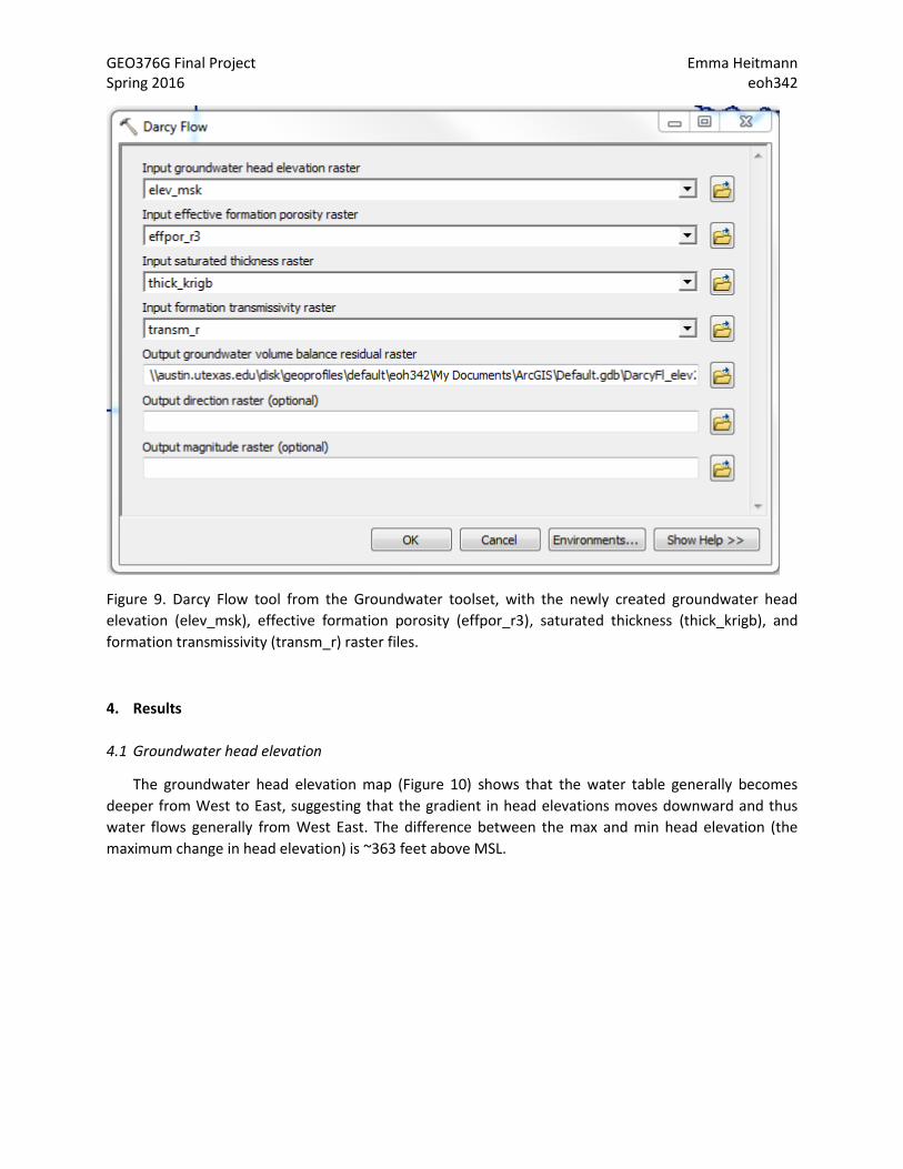
The groundwater head elevation, saturated thickness, formation transmissivity, and effective

porosity raster files were then entered into the “Darcy Flow” tool in the Spatial Analyst – Groundwater

toolset to create a raster with calculated volumetric flux at each cell (Figure 9.)

3.4 Geochemical spatial variability

To map water quality data, water quality reports for the wells had to be downloaded separately,

exported in ArcCatalog to a geodatabase file, then joined to the attribute table of the well shape file (same

process as described for groundwater head elevation). Geochemical parameters were then interpolated

using the “Kriging” tool in the Spatial Analyst toolset by the same process as described for the

groundwater head elevation raster. A Na concentration (ppm) and a Cl concentration (ppm) raster files

were created, and then using the raster calculator added together to create a raster of Na and Cl

concentrations as a proxy for salinity.


Figure 9. Darcy Flow tool from the Groundwater toolset, with the newly created groundwater head

elevation (elev_msk), effective formation porosity (effpor_r3), saturated thickness (thick_krigb), and

formation transmissivity (transm_r) raster files.

4. Results

4.1 Groundwater head elevation

The groundwater head elevation map (Figure 10) shows that the water table generally becomes

deeper from West to East, suggesting that the gradient in head elevations moves downward and thus

water flows generally from West East. The difference between the max and min head elevation (the

maximum change in head elevation) is ~363 feet above MSL.


Figure 10. Map of interpolated groundwater elevations in the Queen City Aquifer, TX.


4.2 Saturated thickness and formation transmissivity

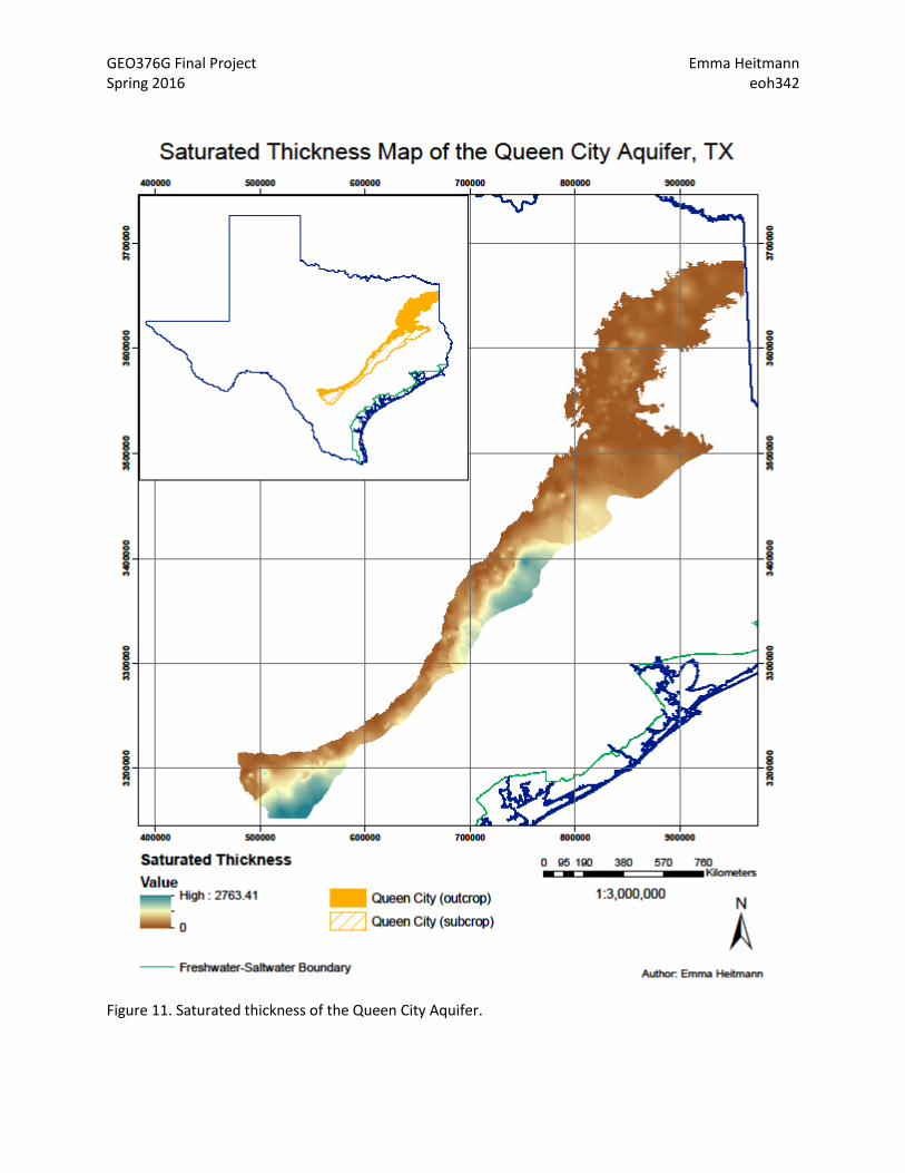
Saturated thickness (figure 11) and formation transmissivity (figure 12) show similar spatial variability,

because the transmissivity map is the saturated thickness multiplied by the assumed constant hydraulic

conductivity of 10-7. The saturated thickness and transmissivity is highest in the Southeast corners of the

aquifer, and decreases in the southeast to northwest trend. The northern portion of the aquifer has a

relatively thin saturated thickness and thus small transmissivity. The maximum saturated thickness

(transmissivity) is 2,763 ft (0.0002763), and the minimum is for both is 0.


Figure 11. Saturated thickness of the Queen City Aquifer.


Figure 12. Transmissivity of the Queen City Aquifer.


4.3 Darcy Flow Analysis

The Darcy Flow analysis (Figure 13) shows volumetric flux of groundwater in a cell, where a positive

value (blue) indicates that water would flow into the cell, a negative value (red) indicates that water would

flow out of the cell, and a value of 0 (green) indicates that there was no net loss of water in the cell. The

results suggest that there is little flow within the aquifer, and that there are no apparent trends in cells

that have a positive volumetric balance and those that have a negative volumetric balance.



Geochemical spatial analysis seemed to show relative variability across the aquifer region. The Ca

concentration (ppm) map (Figure 14) shows that Ca concentrations are generally highest in the Southwest.

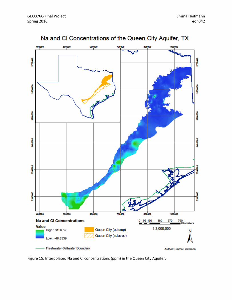
The maximum and minimum interpolated Ca concentrations (ppm) are 287 and -2.3. The Na and Cl

concentration (ppm) map (Figure 15) shows that there are higher concentrations of both in the

southeastern, deepest, and thickest parts of the aquifer. The maximum and minimum interpolated Na

and Cl concentrations (ppm) are 3156 and -46. The pH map (Figure 16) shows that the northern region

and the southeastern corner are generally more acidic, and the interpolated pH values range from 0-9.

The Total Dissolved Solids (m/L) map (Figure 17) shows that TDS generally increases from North to South,

and is highest in the Southeast region. The interpolated values of TDS range from 51 to 2263 mg/L.


Figure 14. Interpolated Ca concentrations (ppm) in the Queen City aquifer.


Figure 15. Interpolated Na and Cl concentrations (ppm) in the Queen City Aquifer.


Figure 16. Interpolated pH values of the Queen City Aquifer.


Figure 16. Interpolated Total Dissolved Solids (mg/L) in the Queen City Aquifer.


5. Discussion

5.1 Groundwater flow

The groundwater head elevation surface suggests that water flows down gradient from West to East.

The maximum saturated thickness of ~2,763 feet is reasonable, as the unit is known to reach thicknesses

greater than ~2,000 feet. The minimum of 0 may be true or may also be due to insufficient well data, or

outdated well data. The effective porosity and hydraulic conductivity values were assumed to be uniform

throughout the aquifer but are unlikely to be uniform in reality, as there is orders of magnitude variability

in the hydraulic conductivities and effective porosities of the various media known to be in the Queen City

Aquifer. Thus these assumption most likely produced error. This error likely carried over into the Darcy

Flow calculator, which was produced a generally uniform volumetric flux surface.


A peak in Ca concentrations in the southwest suggests that Ca concentrations are higher closer to the

recharge point (higher groundwater elevation head), and that they decrease down gradient. Variation in

Ca concentrations may also indicate variation in water source or geologic variability in the system, perhaps

there are more Ca bearing minerals in the southern region of the Queen City sand than the northern

region. A decrease in Ca concentrations along the flowpath of the aquifer may also suggest that chemical

reactions, such as ion exchange, might be occurring to remove Ca from solution. However, the negative

Ca concentrations reported in some areas suggests that the interpolation model at best shows relative

changes in concentrations rather than realistic values.

A high concentration of Na and Cl concentrations in the southeast corners of the aquifer suggest that

there is an overall increase in salinity from the North to the South. The high Na and Cl concentrations may

be due to evaporation or halite dissolution, but in the southeast region is likely due to seawater mixing.

However, the negative Na and Cl concentrations reported in some areas suggests that the interpolation

model at best shows relative changes in concentrations rather than realistic values.

The pH map shows that in general the northern and southern most regions are more acidic than the

central region of the aquifer. The interpolated values suggests very strong acidity in some areas (values

range from 0-9). However, pH less than ~4 is very unlikely in a natural setting, especially in a freshwater

carbonate buffered aquifer. These low values may be due to interpolation methods and/or poor quality

data from some points. However, it does show an overall general relationship that is consistent with other

findings for the aquifer.

The total dissolved solids (mg/L) map shows that the highest TDS is in the southern region, which is

consistent with the Ca, Na and Cl concentrations maps. This may also suggest that this water is older, and

has had longer rock-water interaction time. In general, the interpolated chemical parameters likely have

large error bars, as they produce unreasonable values in some areas. However, the general trends they

show are consistent and plausible in the geologic and hydrologic setting.

6. Conclusions

Groundwater head elevations vary from 130 to 390 feet above MSL, and saturated thickness within

the aquifer is estimated to be up to ~2,763 feet. Groundwater head elevation gradient suggests that water


flows from East to West. There is minimal volumetric fluxes throughout the aquifer, which may be due to

the uniformity of effective porosities and hydraulic conductivities assumed for this model. Geochemical

variations show that Ca concentrations are higher in the Eastern regions, suggesting that Ca may decrease

as water flows down gradient. There is an overall increase in total dissolved solids and salinity from the

North to the South, and that the northern and southern regions are more acidic relative to the central

region.

References

Anders, R.B. Bulletin 5710 – Ground-Water Geology of Wilson County, Texas. U.S. Geological Survey,

1957.

Bear, J. Hydraulics of Groundwater. McGraw-Hill. 1979.

Texas Parks and Wildlife. GIS Data Downloads. http://tpwd.texas.gov/gis/data

Texas Water Development Board. Groundwater Database.

http://www.twdb.texas.gov/groundwater/data/index.asp

http://tpwd.texas.gov/gis/data

http://www.twdb.texas.gov/groundwater/data/index.asp

groundwater flow evaluation and spatial geochemical analysis …€¦ · geo376g final project emma...

Documents