groundwater model review report 11-18-13

SITE-WIDE GROUNDWATER MODEL REVIEW FOR THE UNITED STATES DEPARTMENT OF ENERGY (DOE) PORTSMOUTH GASEOUS DIFFUSION PLANT (PORTS),

PIKETON, OHIO

Natalie Kruse, Dina Lopez, Jennifer Bowman, Aaron Cranford,

Bob Eichenberg, and Gary Conley

Sponsored by Ohio University’s PORTSfuture Project

The PORTSfuture project is funded by a grant from the U.S. Department of Energy Office of Environmental Management Portsmouth/Paducah Project Office

______________________________________________________________________________Site-Wide Groundwater Model Review i

Contents1. Introduction ..................................................................................................................... 1

1.1 PORTS Background .................................................................................................. 2

1.1.1 PORTS Site Geology .......................................................................................... 4

1.1.2 Groundwater Use ................................................................................................ 7

1.1.3 Sources of Groundwater pollution at PORTS .................................................. 10

1.2 Previous PORTS Modeling Efforts ......................................................................... 13

1.2.1 PORTS Modeling Program Needs and Goals .................................................. 13

1.2.2 PORTS Modeling Program Framework ........................................................... 13

1.3 Groundwater Model Codes Used at PORTS ........................................................... 14

2. Recalibrated Model ....................................................................................................... 16

2.1 Purpose of the recalibrated model ........................................................................... 16

2.2 Background of the recalibrated model. ................................................................... 16

2.3 Conceptual Model ................................................................................................... 16

2.3.1 Introduction ...................................................................................................... 16

2.3.2 Approach .......................................................................................................... 17

2.4 Numerical Model ..................................................................................................... 19

2.4.1 Introduction ...................................................................................................... 19

2.4.2 Approach .......................................................................................................... 19

2.4.3 Calibration ........................................................................................................ 23

2.4.4 Validation ......................................................................................................... 26

3. Recalibrated Model Evaluation ..................................................................................... 27

3.1 Stream Discharge Measurement and Water Balance .............................................. 27

3.2 Hydraulic Conductivity ........................................................................................... 28

3.3 Calibration Period ................................................................................................... 35

3.4 Soil and Fill Compaction ......................................................................................... 37

3.5 Model boundaries and Numerical Error .................................................................. 38

4. Recommendations and Conclusions ............................................................................. 40

5. References ..................................................................................................................... 41

1. Introduction

______________________________________________________________________________Site-Wide Groundwater Model Review 1

1. Introduction

The purpose of this report is to serve as a summary and independent review of the Recalibrated Sitewide Groundwater Model for the United States Department of Energy Portsmouth Gaseous Diffusion Plant (PORTS) (DOE 2012b). The Sitewide Groundwater Model is a part of a larger modeling effort on the PORTS site to serve as the basis for decision making during decontamination and decommissioning. The 2006 Sitewide Groundwater Model was recalibrated in 2011 and 2012 (DOE 2012b) and will be used in the groundwater remediation and the Future Conditions Sitewide Groundwater Model; a flowchart of the modeling approach for PORTS is shown in Figure 1.1 (DOE 2011a).

Figure 1.1. Flowchart of the modeling approach at PORTS (DOE 2011a)

This report is structured in four sections. The sections include a general introduction to review the geological and hydrogeological data used in the modeling approaches (Section 1), a summary of the Recalibrated Sitewide Groundwater Modeling approach (Section 2), an

1. Introduction


evaluation of the physical model and the results of the numerical recalibrated model (Section 3), and recommendations and conclusions (Section 4).

1.1 PORTS Background The Portsmouth Gaseous Diffusion Plant (PORTS) facility is located in rural Pike

County, near Piketon Ohio on a 3,777 acre site (Figure 1.2). The location of the approximate centroid of the PORTS facilities is 39.0087°N and -83.0004°W. The site is two miles east of the Scioto River in a small valley running parallel to and approximately 120 feet above the Scioto River floodplain. Figure 1.3 depicts the plant site and its surroundings.

Figure 1.2. Location of PORTS in Ohio

1. Introduction


Figure 1.3. Regional Map Surrounding PORTS

Pike County has approximately 27,700 residents as of 2010. Scattered rural development

is typical; however, the county contains a number of small villages such as Piketon and Beaver that lie within a few miles of the plant. The county’s largest community, Waverly, is about 10 miles north of the plant and has a population of about 4,400 residents. The nearest residential center in this area is Piketon, which is about 5 miles north of the plant on U.S. Route 23 with a population of about 1,900. Several residences are adjacent to the southern half of the eastern boundary of the plant and along Wakefield Mound Road (old U.S. 23), directly west of the plant (DOE 2012a).

PORTS, which produced enriched uranium via the gaseous diffusion process from 1954 through 2001, is owned by the U.S. Department of Energy (DOE). In 1993, DOE leased the uranium production facilities at the site to United States Enrichment Corporation (USEC), a private corporation that produced enriched uranium for use in nuclear power plants. DOE is responsible for decontamination and decommissioning (D&D) of the gaseous diffusion process buildings and associated facilities, environmental restoration, waste management, uranium operations, and management of facilities that are not leased to USEC.

1. Introduction


The PORTS facility has been subjected to several hydrogeological studies and modeling efforts. The last of these modeling works was the recalibrated sitewide groundwater model (DOE 2012b). Contamination in the form of chlorinated solvents perchloroethylene, trichloroethylene, and dichloroethylene (PCE, TCE, DCE) have been identified in the aquifers of the PORTS site. The purpose of this report is to review this last groundwater flow model and comment about its strengths and weaknesses.

1.1.1 PORTS Site Geology PORTS is located within the Knobs-Lower Scioto Dissected Plateau portion of the

Western Allegheny Plateau Physiographic Ecoregion. The bedrock geology units that outcrop in this region were deposited between the late Devonian through the late Mississippian Periods. The Bedford Shale and Berea Sandstone are the oldest strata known to outcrop at PORTS. These outcrops are present within the deeply incised streams and valleys throughout the PORTS reservation (USEC 2004). The Mississippian-aged Sunbury Shale and Cuyahoga Formation overlay the Devonian-aged Bedford and Berea formations. The Sunbury Shale apparently thins westward as a result of erosion by the ancient Portsmouth River, and is absent on the western half of the site (USACE 1993). The Sunbury Shale also is absent in the drainage of Little Beaver Creek downstream of the Lime Sludge Lagoons and the southern portion of Big Run Creek, where it has been removed by erosion. The Cuyahoga Formation, the youngest and uppermost bedrock unit at PORTS, forms the hills surrounding the site, particularly to the east. It has been eroded from other portions of the site, however regionally it can reach thicknesses of 160 ft (USEC 2004).

The geologic structure of the area is dominated by relatively flat-lying Paleozoic shale and sandstones that are overlain by the more recent Pleistocene fluvial and lacustrine deposits (Slucher 2006). The PORTS site spans across a valley created by the paleochannel of the Portsmouth River, a tributary to the Teays River. A large meander of the Portsmouth River flowed through the PORTS site, cutting through the Cuyahoga Formation and into the Sunbury Shale and Berea Sandstone (USACE 1993). It deposited the fluvial silt, sand, and gravel of the Gallia Sand Member of the Teays Formation that underlies most of the PORTS industrial complex within Perimeter Road and areas south and southeast of the reservation. The plant site is located primarily within this channel, underlain by unconsolidated sediments of the Teays River Valley system, as seen in Figure 1.4. The geology of the PORTS site is formed by two distinct units—the consolidated sedimentary structures and the unconsolidated strata of the paleochannel (Figure 1.5). The hydraulic conductivity of the unconsolidated Gallia Sand causes it to be the primary geologic strata to contain groundwater and transport contaminants. The Gallia Sand is confined from the underlying consolidated Berea Sandstone, another water bearing unit, by the discontinuous Sunbury Shale layer. The Gallia Aquifer contains the majority of the groundwater contamination from the PORTS site, although some contamination has also migrated into the underlying Sunbury Shale layer. The groundwater contamination primarily consists of dense non-aqueous phase liquids, namely chlorinated solvents including trichloroethylene and its bi-products (i.e. DCE, vinyl chloride, etc.) (DOE 1990).

1. Introduction


Figure 1.4. Unconsolidated geology near PORTS

1. Introduction


Figure 1.5. Cross section of PORTS site located above the unconsolidated alluvium of the

Portsmouth River, part of the Teays River system (DOE 2012).

Beyond the boundary of the plant site, the DOE property continues onto the hillsides surrounding the Portsmouth River Channel valley structure. The valley is oriented north to south and is bounded on the east and west by ridges or low-lying hills that have been deeply dissected by present and past drainage features. These ridges consist of Mississippian formations of Sunbury and Cuyahoga Formations. While there is limited water in the upland shales, existing mostly in perched aquifers, they tend to be lower permeability than the unconsolidated zones. Another significant landform is the small valley formed by Little Beaver Creek, which flows northwesterly across the middle of the DOE property, just north and east of the industrial area of the plant (DOE 1990).

The hydrogeologic conditions underlying the DOE site are similar to those of the Teays River Valley. The shale and sandstone bedrock underlies the entire property and outcrops in the hills along the east and west portions of the facility. The unconsolidated alluvial deposits are the Minford Clays and the Gallia Sand formations. A moderate amount of free water is contained in the gravelly Gallia Sand but is not easily obtainable because of the large percentage of clay mixed in the gravel. The Minford Clays are essentially impermeable except in the weathered surface layers (OEPA 1990).

An analysis of topographic maps, surface water drainage, and past aerial photos of the site led to the prediction of groundwater divides and an interpretation of groundwater flow directions (Figure 1.7). PORTS is divided into several zones for monitoring and remediation as illustrated in Figure 1.6. Inspection of Figures 1.6 and 1.7 shows that groundwater in the

1. Introduction


northern part of the site flows toward Little Beaver Creek, Quadrant IV. Little Beaver Creek is a tributary to Big Beaver Creek which then drains into the Scioto River west of PORTS. In the vicinity of the X-701B Holding Pond Monitoring Area (eastern portion of the site), groundwater flows eastward toward the headwaters of Little Beaver Creek, Quadrant II. The flow direction at X-740 and Chromium Sludge Surface Impoundment Area, is westward toward a small, unnamed, intermittent tributary of the Scioto River, Quadrant III. Subsurface flow at X-749, Contaminated Materials Disposal Facility, is divided between a westward component and an eastward component conforming to the upper reaches of the Big Run drainage basin Quadrant I. The upper tributaries of Big Run drain the area of X-231B, Oil Biodegradation Plot. Groundwater flow in this flat area is likely toward the south (DOE 2010).

1.1.2 Groundwater Use Two water-bearing aquifers are present beneath PORTS: the Gallia Sand and the Berea

Sandstone formations. The Gallia is the uppermost aquifer below the PORTS infrastructure while the Berea Sandstone is deeper typically separated from the Gallia Sand by the Sunbury Shale acting as a barrier to vertical groundwater flow. However, in some areas the Sunbury Shale has been eroded and the Gallia overlies the Berea Sandstone. The Minford Member overlies the Gallia Sand and is hydraulically connected. The Minford Member acts as a vertical contaminant pathway to the Gallia Sand, which is the most permeable unit at the site and the primary pathway of contaminant migration to Little Beaver Creek and Big Run. The groundwater flow beneath PORTS is dissected and flows towards one of the various drainage areas (i.e. Little Beaver Creek, West Drainage Ditch, and Big Run), thus dividing the site into multiple quadrants or areas of general flow direction (Figure 1.7). Many extraction wells have been drilled for treatment of groundwater contamination and to alter contaminant plume migration. These wells affect groundwater flow within their areas of influence.

Figure 1.8 shows a stratigraphic section of the PORTS site; the Gallia Sand being an unconsolidated sand and gravel layer that has the highest hydraulic conductivity.

1. Introduction


Figure 1.6. Dissected Gallia groundwater flow direction beneath PORTS (DOE 2008).

1. Introduction


Figure 1.7. Dissected Berea groundwater flow direction beneath PORTS (DOE 2008).

1. Introduction


Figure 1.8. Stratigraphic profile of the unconsolidated and consolidated geologic units

underlying the PORTS site (Provided by J.D. Chiou 2012).

1.1.3 Sources of Groundwater pollution at PORTS According to the 2010 Annual Site-wide Evaluation Report (DOE 2012a), there are twelve

areas monitored for potenial groundwater contamination, these areas are analyzed for metals, volatile organic compounds (VOCs), and/or radionuclides. Five of these areas have known groundwater contamination plumes. Contamination in these plumes consists of volatile organic compounds (mostly TCE) and radionuclides (Technetium). These twelve areas are shown on Figure 1.9. and listed below:

Quadrant I o X-749/X-120 (plume) o Quadrant I Groundwater Investigative Area (plume)

Quadrant II o Quadrant II Groundwater Investigative Area (plume) o X-701B Holiding Pond (plume)

Quadrant III o X-616 Chromium Sludge Surface Impoundments o X-740 Waste Oil handling Facility (plume)

Quadrant IV o X-611A Former Lime Sludge Lagoons o X-633 Pumphouse/Cooling Towers Area

1. Introduction


o X-735 Landfills o X-734 Landfills o X-533 Switchyard Area o Former X-344C Hydrogen Fluoride Storage Building

1. Introduction


Figure 1.9. Groundwater investigation and monitoring areas at PORTS (DOE 2012a).

1. Introduction


1.2 Previous PORTS Modeling Efforts There have been numerous analytical and numerical models developed for PORTS over the past 25 years. In the 1980’s, simple analytical and Random-Walk models were used to track plume movement at PORTS. The analytical models used in the 1980’s were followed by more complex numerical models in the 1990’s. In the 1990’s, a more complex approach was taken using finite difference methods or finite element methods. These methods included models developed using MODFLOW (Harbaugh et al. 2000), MODPATH (Pollock 1994), and MT3D (Zheng 1990). The objective of these first models was to support the RCRA Facility Investigation (RFI) for Quadrant Phase I and II, investigate fate and transport of contaminants (primarily TCE), and investigate the groundwater system under typical and reasonable maximum exposure scenarios. Other models, including FRAC3DVS, MAGNAS3, and UTCHEM, were also used for evaluation of remedial alternative for PORTS (DOE 2011b). In 2006, a sitewide groundwater numerical model using the MODFLOW modeling framework was created. The purpose of the 2006 model was assessment for site planning and impact assessment. The 2006 model was developed using some of the work developed through previous modeling and became a tool for evaluating effectiveness of actions. The 2006 model had some serious limitations, including the model domain size, sparse data in some parts of the model domain, limited data for the model calibration and oversimplified assumptions about recharge. The model reviewed in this report is the 2011 and 2012, which is a recalibration of the 2006 model to reflect new data and add more detail to the model, reflecting a major improvement in PORTS modeling (DOE 2012b).

1.2.1 PORTS Modeling Program Needs and Goals On the PORTS site, multiple models are necessary to facilitate decision making during

decontamination and decommissioning. As shown in Figure 1.1, many systems have been modeled, are being modeled, or are proposed to be modeled on site including (DOE 2011a):

Groundwater, surface water, soil remediation OSDC (On-site disposal cell) siting Waste acceptance criteria development (WAC) Performance assessment/composite analysis (DOE Order 435.10) OSDC operations

The results from these models are being used to make decisions during decontamination

and decommissioning. These models are also being used as framework for the detailed evaluation of response action as part of a decision documents to select the most appropriate site remedy.

1.2.2 PORTS Modeling Program Framework The modeling framework for the PORTS site is complex and interlinked. In the revised

model, previous and ongoing monitoring data have been added. This includes information that has been added to the quadrant-specific area models and the current condition sitewide groundwater model. The development of cleanup goals relies on the combination of the future

1. Introduction


condition sitewide surface water model and the future condition sitewide groundwater model. Data for surface water modeling include future land condition assumptions and data collected during geotechnical and geochemical investigation (DOE 2011a).

OSDC numerical WAC (waste acceptance criteria) rely on several model development aspects including the future condition sitewide groundwater model, source area specific vadose zone model, and engineering and leaching geochemical investigations. All of this requires data and information from an OSDC design. Modeling for groundwater remediation, soil remediation goals, and OSDC numerical WAC will provide input into the CA (composite analysis) and PA (performance assessment) (DOE 2011a).

1.3 Groundwater Model Codes Used at PORTS The selected model code for the sitewide groundwater model for PORTS needed to be

appropriate for the site, be available to the public domain, be actively maintained or upgraded, be commonly applied, and be accepted by regulators. The modeling codes used for the recalibrated sitewide model include MODFLOW 2000 for groundwater flow, MT3DMS for mass transport, and MODPATH for groundwater particle tracking. Groundwater Vistas by Environmental Solutions operates the codes within a graphical user interface (DOE 2012b).

1.3.3.1 MODFLOW and MODPATH MODFLOW was chosen because it is in the public domain, widely used by industrial,

scientific, and governmental communities, rigorously tested and verified, and a variety of tools are publicly available for graphical preprocessing and post-processing. It was used for the 2006 current PORTS sitewide groundwater flow model. MODFLOW simulates transient and steady-state saturated flow in 1, 2, or 3 dimensions. MODFLOW calculates potentiometric head distribution, flow rates, velocities, and water balances in an aquifer. It can simulate aquifers as unconfined, confined, or a combination of both. Models for recharge, flow toward wells, groundwater discharge into drains and water exchange with rivers are all included in MODFLOW (DOE 2011a).

MODPATH is a three-dimensional particle tracking post-processing program that uses a semi-analytical particle-tracking scheme and is designed for use with a steady-state simulation output from MODFLOW. MODPATH can compute 3-D path lines, positions of particles at specified points in time, discharge point coordinates, and total time of travel for each particle. Based on the assumption that each directional velocity component varies linearly within a grid cell in its own coordinate direction, allows for an analytical expression to be obtained and the path of the particle within the cell can be calculated. By describing flow path within a grid cell, the time of travel between points can be computed (DOE 2011a).

1.3.3.2 MT3D MT3D is a comprehensive 3D numerical model for simulating solute transport in

complex hydrogeologic settings. It models the fate and transport of dissolved, single or multiple species contaminants in saturated groundwater. The MT3D model calculates concentration

1. Introduction


distributions, concentration histories at selected receptor points and hydraulic sinks, and the mass of contaminants in ground water. MT3D can simulate 3D transport in complex steady-state and transient flow fields and includes terms for anisotropic dispersion, sources-sinks, and chemical reaction such as first order transformation reactions and linear and nonlinear sorption. When linked to MODFLOW it can model advectively dominated transport problems as well as models that include dispersion and the reactions mentioned previously (DOE 2011a).

2. Recalibrated Model



2.1 Purpose of the recalibrated model After 25 years of modeling efforts at PORTS to support decision making, in 2006, a

sitewide groundwater model was developed by CDMJV (CDM, Joint Venture) for large-scale impact assessment and planning level decision making. Previous models had focused on specific areas of the site. Results from previous modeling projects have been used to develop the sitewide model. The sitewide model was then used to create four area-specific models with finer modeling grids. The telescopic mesh method was used for that purpose. In this method, results from the sitewide model can be used as boundary conditions for the smaller area-specific models. The sitewide model and area-specific models were refined and recalibrated during the Fall and Winter of 2011. The recalibrated model is evaluated here.

The purpose of the sitewide model is to support planning level and large scale impact assessment; more recently the model has also been used to support OSDC waste acceptance criteria (WAC) development. The model purpose is the evaluation of long term protection of human health and the environment. The recalibrated model will form the basis for estimation of future hydrologic conditions as the surface is altered and contamination sources are removed.

2.2 Background of the recalibrated model. The recalibrated site-wide model and the associate area-specific models for the X-740

area, X-749 area, Quad II and Quad IV are a refinement of the 2006 models. The update and recalibration incorporated recent investigations from the potential OSDC sites and available surface water flow data. Information from the area-specific models was added into the site-wide model. The model was recalibrated by first assessing the original calibration period for representativeness before updating the calibration to current (2011) site conditions. The model was then validated using additional water level datasets for three different dates. The recalibration has followed Ohio EPA and ASTM guidance. The information that follows in sections 2.3 and 2.4 is based on the model documentation (DOE 2012b).

2.3 Conceptual Model

2.3.1 Introduction The conceptual model is based upon the hydrostratigraphy, groundwater recharge and

discharge and groundwater flow in the model domain. The model domain extends north to Big Beaver Creek and south, east and west beyond the DOE property line; the model domain encompasses the DOE property and the plant area. The plant area refers to the area which is inside perimeter rode.

PORTS is located in the Appalachian Plateau, just beyond the limit of glaciation. The plant area straddles a mile-wide ancient river valley created by the Portsmouth River. The Portsmouth River, a part of the ancient Teays River system, partially eroded the upper bedrock layers: the Cuyahoga Formation, the Sunbury shale and the Berea sandstone. The Bedford shale



which underlies the Berea sandstone was uneroded by the river. The Portsmouth River deposited fluvial sediments creating the unconsolidated Gallia (Gallia sand and gravel) member. The Portsmouth River was blocked by advancing glacier and lacustrine silts and clays deposited in the lake creating the Minford member (Minford silt and Minford clay) of the Teays formation. The current plant area surface is the result of cut and fill during plant operation which filled depressions and leveled knolls.

The Gallia sand and gravel is the main water bearing unit in the model domain. The Minford silt is slightly less hydraulically conductive than the Gallia sand and gravel, but is more conductive than the Minford clay. The Sunbury shale acts as a confining layer over the Berea Sandstone where the shale is greater than 4 feet thick. The Berea sandstone is water bearing with a hydraulic conductivity lower than the Gallia sand and gravel. The Bedford shale acts as the deepest confining layer of the hydrologic system due to its low hydraulic conductivity and thickness.

The groundwater recharge to the model domain is primarily from precipitation. Differential recharge rates are applied across the model domain to take the following into account: a) impervious surfaces within Perimeter Road, b) reduced recharge at the base of Cuyahoga Formation slopes due to increased runoff and c) the average recharge across the remainder of the model domain.

2.3.2 Approach

2.3.2.1 Stratigraphy The stratigraphy of the model domain has been represented in the conceptual model with

both unconsolidated and consolidated formations. From the oldest formations, the Bedford shale represents the bottom of the model domain; it is thick and continuous across the model domain. The Bedford shale has a low enough conductivity for the layer to serve as the lower model boundary. The Berea sandstone overlies the Bedford shale. It is continuous underneath the entire DOE property. The Berea sandstone consists of two units, the upper 10 to 15 feet is fine-grained sandstone and the lower 5 to 20 feet includes interlayered shale laminations similar to the Bedford shale. The Sunbury shale is the uppermost bedrock layer underlying the broad valley in which the plant area lies. In portions of the DOE property, the ancient Portsmouth River eroded the Sunbury shale; in those areas, the Berea sandstone is the uppermost bedrock unit. The Cuyahoga Formation is the uppermost bedrock unit across the DOE property (but not under the plant area). It is thinly laminated shale that forms the hills that surround the broad fluvial-lacustrine valley in which the plant area is located. The formation has been eroded beneath the plant area.

The unconsolidated strata that underlies the plant area is the result of the fluvial and lacustrine deposits from the ancient Portsmouth River. The Gallia sand and gravel is the lower of the unconsolidated members. It is discontinuous across the DOE property and is typically less than 10 feet thick in the model domain. The poorly sorted nature of the Gallia sand and gravel is typical of the meandering river that deposited it. The Minford member is the lacustrine deposit



that overlies the Gallia and consists of two units. The upper unit, the Minford clay, is mostly clay with some fine sand. The lower unit, the Minford silt, is clayey silt and fine-grained sand. The Minford member is continuous beneath the plant area. The soil within the DOE property consists of recent alluvium, loess and colluvium in addition to fill used to level the plant area. Up to 20 feet of fill was used to level the plant area.

2.3.2.2 Aquifer Properties The Gallia is the main contaminant pathway with the highest hydraulic conductivity,

although the hydraulic conductivity of the Gallia is highly variable due to its poorly sorted nature. The Berea sandstone is the only bedrock layer in the model domain that is considered to be water-bearing. The shales and clays on site act as confining units, including the Minford Clay, the Cuyahoga Formation, the Sunbury shale, and the Bedford shale. Where the Sunbury shale is intact, it limits downward migration from the Gallia to the Berea sandstone; where the Sunbury shale is eroded, the Gallia is hydraulically connected to the Berea sandstone. The hydraulic conductivity of the Gallia varies from 0.01 to 150 feet per day, the Berea is an order of magnitude less conductive, varying from 0.004 to 15 feet per day. The hydraulic conductivity of the Minford varies 0.1 to 2 feet per day and the Sunbury shale varies from 0.0001 to 0.01 feet per day.

2.3.2.3 Groundwater Recharge Recharge to the system is from precipitation; recharge has been previously estimated to

vary from 8.9 to 13.9 inches per year, disregarding reduced recharge due to impervious surfaces and storm sewers, streams and rivers. In previous groundwater models of PORTS, a recharge rate of 4 inches per year was applied across the model domain with a decreased value in building locations. In the recalibrated model, the recharge at the toe of Cuyahoga Formation slopes is higher where the slope meets the Minford member, while the recharge on the slopes is lower due to runoff. There is a minimal amount of recharge from leaking cooling and transmission water lines, although the rates are unknown.

2.3.2.4 Groundwater Discharge Groundwater discharges to several streams in the model domain including Little Beaver

Creek in the north and east, Big Run Creek in the south, the Southwestern Drainage Ditch in the southwest, the East Drainage Ditch in the east and the West Drainage Ditch in the west.

2.3.2.5 Groundwater Flow and Boundary Conditions Major flow boundaries include Little Beaver Creek, Big Run Creek, the Southwestern

Drainage Ditch, the East Drainage Ditch and the West Drainage Ditch. Other discharge points include extraction wells, sumps and phytoremediation systems. Groundwater flow in the DOE property is generally towards discharge locations. All surface water is part of the Scioto River drainage basin. Streams and drainage ditches dissect the Minford, Gallia, Sunbury and, in places, the Berea formations.



2.4 Numerical Model

2.4.1 Introduction The numerical model was developed using on-site investigations and past models. The

current generation of the model was developed through reconfiguration of the 2006 sitewide model. The new model incorporates new boring investigation data from the potential OSDC site, data from the area-specific models, other updates to match the conceptual model better, add additional site information and improve boundary conditions.

2.4.2 Approach

2.4.2.1 Model Updates and Reconfiguration Data from new wells installed in Fall 2011 in the northeast and southeast portions of the

DOE property were added to the model. Data was scaled based on a ratio between conditions during measurement and conditions during the calibration timeframe. Recharge to Cuyahoga outcrops was reduced while the recharge at the base or permeable contact of Cuyahoga outcrop areas was increased to reflect field data. Additionally, the representation of outcrops was modified, the model domain was expanded, boundary conditions were changed (see Figure 2.1), additional zones of conductivity were added to the Gallia and Berea (see example shown in Figure 2.2), conductivity zones near streams were improved and model recharge was changed to reflect the presence of buildings and parking lots. The land surface was added to the model, however, MODFLOW does not use the land surface for modeling, only for visualization.



Figure 2.1. Boundary conditions used in the recalibrated sitewide groundwater flow model

(DOE 2012b)



Figure 2.2. Hydraulic conductivity zones in Layer 1 of the recalibrated sitewide groundwater

flow model (DOE 2012b)

2.4.2.2 Model Code The sitewide model was created in MODFLOW 2000 with the graphical user interface,

Groundwater Vistas.



2.4.2.3 Model Area and Grid The model domain represents 18.2 square miles and extends from 1093 feet above mean

sea level to 500 feet above mean sea level. The domain, shown in Figure 2.3, was expanded to enable as many natural flow boundaries as possible and, where necessary, general head boundaries can be far enough away from the DOE property to not affect water levels in the DOE property.

The model grid spacing is variable throughout the model domain. The grid consists of 552 rows and 372 columns with a minimum spacing of 17 feet and a maximum spacing of 234 feet. Spacing is smaller near the TCE plumes and larger near the model boundary.

Figure 2.3. Model domain (DOE 2012b)



2.4.2.4 Model Stratigraphy The PORTS stratigraphy was divided into six layers. Where the Cuyahoga Formation is

absent, the model layers represent the Minford Formation, the Gallia Formation, the Sunbury Shale, the upper Berea Sandstone, the lower Berea Sandstone and the Bedford Shale. Where the Cuyahoga Formation is present, the Minford and Gallia Formations are absent, so the top two layers represent the Cuyahoga Formation. In areas where the Sunbury Shale is eroded, the third layer represents the Gallia Formation. Where the stratigraphy is incised by streams, the model layers represent alluvium, as found in the field. The thickness of each layer was determined from site borings.

2.4.2.5 Boundary Conditions Two types of boundary conditions have been used in the sitewide groundwater model:

specific flux and head-dependent boundary conditions. Specific flux boundaries are used to represent flow boundaries—positive flux to simulate recharge, negative flux to simulate production wells and no flux in areas of no groundwater flow. Head-dependent boundaries include drains, rivers and general head boundaries.

Specific flow boundaries were used to apply recharge to different recharge zones. The recharge areas are those covered by Minford/Gallia deposits, the base of the Cuyahoga outcrops, the Cuyahoga outcrops, buildings, parking lots and landfills. Additional recharge was added in the area of the former cooling towers. Small zones of increased recharge from the area-specific models were added to the sitewide model adjacent to the X-749 and Peter Kewitt landfills. Extraction wells and sumps were modeled as individual wells (a type of specific flow boundary); the well rates modeled were measured in late summer 2007. The flow rate of the phytoremediation system was based on one half of the design extraction because the trees are halfway to maturity. No flow boundaries were used for the north side of Big Beaver Creek (see Figure 2.1), where model layers extend into stream valleys, and the bottom of the model domain.

Head-dependent boundaries include rivers, drains and general head boundaries. Big Beaver Creek has been modeled as a river, while the other, smaller creeks have been modeled as drains. One pond (X-230J7) was also simulated using a river boundary, although to achieve good calibration a low permeability bottom was added to the pond. General head boundaries were used on the east and south boundaries of the model domain in the Berea sandstone and the Bedford shale to allow groundwater to flow to the south and southeast to match field data. The general head boundaries were set based on hydraulic gradients extrapolated to the boundaries of the model domain. The reconfigured model boundary matches the natural contour rather than a ninety degree angle. General head boundaries were also used for the ponds on DOE property, besides the X-230J7 pond; the heads were set to the known elevation of the water surface of each pond.

2.4.3 Calibration The new reconfigured model was calibrated to the original model calibration target of

October 2006 measured groundwater levels, with the addition of new wells in the proposed



locations of the on-site disposal cell and a secondary target of Little Beaver Creek flow rate. Vertical and horizontal hydraulic conductivities and recharge rates were adjusted within reasonable ranges to achieve agreement between simulated and measured groundwater levels.

The calibration period was selected due to the completeness of the dataset. The October 2006 time period was compared to April 2007, July 2008 and January 2011. While the two months prior to October 2006 were very wet, the eight months prior to August 2006 were unusually dry. The premise of using the period for calibration despite the wet conditions was that the recharge period is longer than two months and that the year preceding the calibration period would be a better reflection of water level. Of the four time periods assessed, the average precipitation in the year prior to October 2006 and January 2011 were drier while April 2007 and July 2008 were wetter. October 2006 was a transition from a drought to a wet period.

Initial parameter values for the reconfigured model were selected from the calibrated hydraulic conductivity and recharge values from the 2006 sitewide groundwater model. An iterative process of heuristic model runs to check model sensitivity and calibration and PEST (Model-Independent Parameter Estimation and Uncertainty Analysis) parameter estimation runs were used to calibrate the model. The recalibrated model, like the 2006 sitewide model included conductivity zones that contained areas with wells that responded similarly; these were delineated based on hydrostratigraphy, topography and well response. Largely, the zones remained the same between the 2006 model and the reconfigured model, but the values changed. As few zones as possible were used to represent the hydrostratigraphy, using one zone per geologic unit, where possible. Both the Gallia and the Berea contained multiple zones. PEST was used to adjust recharge, hydraulic conductivity, and drain conductance.

Calibration was completed to achieve groundwater heads within 5% of observed heads with a residual standard deviation within 10% of the observed heads, two sample calibration plots are shown in Figures 2.4 and 2.5 for the Gallia sand and gravel and the Berea sandstone, respectively. The groundwater flow direction was qualitatively in the same direction as the known plume flow directions. Horizontal and vertical flow gradients matched qualitatively and quantitatively with that seen on site. The mass balance error in MODFLOW was less than 1%. Modeled stream flow rate was approximately half of that estimated in the field (115 gpm modeled, 394 gpm estimated) but the measured stream flow was not the base flow because it was not measured in dry conditions, the difference was attributed to the stream having also overland flow contributions.



Figure 2.4. Calibration results for groundwater head elevations in the Gallia sand and gravel

(DOE 201b)

Figure 2.5. Calibration results for groundwater head elevations in the Berea sandstone (DOE

2012b)

A sensitivity analysis was performed to determine the model’s response to variation in recharge, hydraulic conductivity of the Minford, Gallia, Sunbury and Berea, drain conductance and extraction well pumping rate. Parameters were adjusted by 15% (positive and negative) one at a time. The model is the most sensitive to recharge, then Gallia hydraulic conductivity, then Berea hydraulic conductivity.



2.4.4 Validation The calibrated model was validated against three other datasets to ensure the applicability

of the model for wet and dry periods. The validation was performed by varying only the combined recharge across the model domain and maintaining hydraulic conductivity and other variables at the values included in the calibrated model. The validation periods were April 2007, July 2008 and January 2011, representing average (January 2011) and wet (April 2007 and July 2008) conditions. A 25% increase in recharge was used for April 2007, a 12.5% increase in recharge was used for July 2008 and a 10% increase in recharge was used for July 2011. The water levels in the DOE property were lower in July 2011 than in October 2006, so an increase in recharge is unexpected. Despite this, the validation results were within the validation targets for the model and were considered successful.

3. Recalibrated Model Evaluation



The numerical model that the authors have presented seems to be a reasonable approach in terms of boundary conditions and comparison between the observed and simulated values. It seems to be the result of a long and deep study of the area and the compilation and analysis of a significant amount of data. The calibration errors are relatively high compared to other numerical models of other areas but we need to consider here the high heterogeneity and anisotropy of the modeled layers. It is probably not possible to create a model that can represent all that complexity. The authors seem to have done a good job in simplifying, within reasonable limits, the complexity of the modeled system. However, there are some limitations in the current model that should be addressed or clarified in future modeling in order to support completely the construction of the model and the simulated results. Discussion of limitations identified by Ohio University for inclusion in future modeling is included in this section. This discussion focuses on the following items:

Stream discharge measurement methods

Hydraulic conductivity ranges modeled

Representativeness of the calibration period

Impact of compaction of soil and fills in altered areas on-site

Numerical error from a coarse vertical grid

3.1 Stream Discharge Measurement and Water Balance The secondary calibration target for the reconfigured sitewide groundwater model is the

discharge rate of Little Beaver Creek. While ‘observed’ flow rates have been cited, there is little reference to the estimation or measurement methods. It is not evident from the modeling report if or how the stream discharge was measured. Since this is a calibration target, the measurement or estimation method should be detailed to allow the reader to understand the potential error and the stated success of calibration. The calibration results presented on page 56 show a modeled streamflow of approximately 30% of the observed streamflow; this is cited as being within the error limits of the observed value and the fact that the modeling results are “base flow” instead of total discharge of the stream. The total discharge of the stream includes base flow and overland flow contributions. This calibration is difficult to assess without an understanding of the methods. Measurement of streamflow is well established and could be undertaken with little additional expense.

Little Beaver Creek is an appropriate size to be measured using either a velocity meter on a wading rod (higher discharge) or a cutthroat flume (low discharge). Each method is well established by the United States Geologic Survey (USGS) (Turnipseed and Sauer 2010). Velocity meters are typically either physical or electronic. Physical meters consist of an impeller that spins at a rate proportional to the stream velocity. Rotations are counted for at least forty seconds. The USGS developed the pygmy meter, an impeller velocity meter that is economical and accurate. Electronic meters use either Doppler or electromagnetic field to measure the



average velocity over a 40 second period. A Sontek Acoustic Doppler velocity meter is a commonly used model that provides accuracy and ease of use.

It is clear from this report that a good water balance of the area has not been done. That includes measurements of precipitation, evapotranspiration, infiltration, stream flow. The information generated by water balance could provide important information for the modeling work and better criteria for calibration work. It is recommended that this work be incorporated into any future modeling efforts.

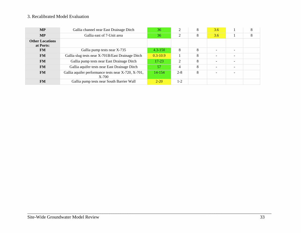
3.2 Hydraulic Conductivity Hydraulic conductivity values are central to the sitewide groundwater flow model. The

model calibration began with hydraulic conductivities from previous modeling studies before recalibration. The recalibrated models were then compared with the initial values to ensure that the new values were in the same range. While the calibration results of the reconfigured model are within the range of acceptable error for its purpose, many hydraulic conductivity values vary significantly from accepted county-wide values published by the Ohio Department of Natural Resources (ODNR 2003). While pumping tests and field measurements on-site are clearly more accurate than county-wide data, it is expected that the values fall close to the ODNR reported values or that the deviation be explained before use as initial values for model calibration. Table 3.1 presents the hydraulic conductivity rating given to each stratigraphic unit in the ODNR publication and Table 3.2 defines the range of hydraulic conductivities that defines each rating. The hydraulic conductivities presented in Table 1 of the Recalibrated Sitewide Groundwater Flow Model Documentation report are duplicated in Table 3.3 alongside the corresponding value assigned by ODNR. The hydraulic conductivities Kz and Kh presented in Table 3.3 correspond to field measurements (FM) or they are hydraulic conductivity calibration values for previous modeling efforts at PORTS, the ratings correspond to the values presented in Table 3.2 (ODNR 2003). The hydraulic conductivities presented in Table 3.4 represent the hydraulic conductivity values in the calibrated model (DOE 2012b). The values are color coded to denote the magnitude of difference between on-site values from field measurements or past models and those assigned in the ODNR report. Typically, the values measured on-site are within two orders of magnitude of the ODNR values, while the larger deviations are seen in the values from previous models. The calibrated model has smaller differences when compared to ODNR values.

While the calibration results of the recalibrated model are not disputed, the difference between ODNR reported values and values from previous models ought to be recognized and explained. The wide range of values reported are difficult for the reader to understand without knowledge of the site. It is recommended that future model documentation be clearer to facilitate public understanding of assumptions.



Table 3.1. Hydraulic conductivity ratings for stratigraphic units in Pike County (ODNR 2003)

Table 3.2. Range of hydraulic conductivity for each rating. The original reference includes no range for ratings of 3, 7 or 9 (ODNR 2003)

Stratigraphic Units Typical Ratings Based on ODNR Report

Gallia (Sand and Gravel) 8

Minford (Silt and Clay) 3

Berea (Sandstone) 6

Cuyahoga (Shale) 3

Sunbury (Shale) 3

Rating Hydraulic Conductivity (ft/day)

1 .134-13.4

2 13.4-40.2

4 40.2-93.8

6 93.8-134

8 134-268 10 268+


___________________________________________________________________________________________________________Site-Wide Groundwater Model Review 30

Table 3.3. Magnitude of difference between hydraulic conductivity values on site and those reported by Ohio Department of Natural Resources (ODNR 2003). The magnitude of difference is color coded; larger differences are coded in red and pink, smaller differences are coded in green and yellow as detailed below. The un-colored cells are outside of the colored ranges.

Magnitude of Difference

10-4-10-3

10-3-10-2

10-2-10-1

10-11

1-10

10-100

100-1000

1000-10000

>100000

Data Type Kh Rating Typical

Rating Kz Rating Typical

Rating X749/X-120 Area:

FM Gallia multiple-well tests near x-231 6.8-62 1-4 8 - - -

FM Gallia slug tests near X-749 1.9-8.4 1 8 - - -

FM Gallia multiple-well tests near X-701B holding pond 24-104 2-6 8 - - -

FM Minford laboratory measurements in X-701B area NA 3 .000026-.00013

- 3

FM Minford single-well aquifer test near X-616 0.62 1 3 - - -

FM Gallia short-term tests near X-749 1.8 1 8 - - -

FM Berea single well aquifer tests .0045-15 1 6 - - -

FM Gallia pump tests in X-749 area: range of values (average)

1-38.44 (5) 1-2 8 - - -

FM Gallia recovery tests in X-749 area: Range of values (average)

0.81-18.88 (4.3)

1-2 8 - - -

MP Berea 0.1 1 6 0.01 - 6

MP Alluvium Zone in Gallia layers in SE corner of model 2.5 1 3 0.25 1 3

MP Alluvium Zone in Minford layers in SE corner of model

2.5 1 3 0.25 1 3



MP X-749 RCRA closure trench 100 6 ? 10 1 ?

MP Gallia zone in western 2/3 of block of mesh added north of PK

13 1 8 1.3 1 8

MP IRM & X-749 RCRA closure slurry walls 0.00006 NA 0.000006 NA

MP Higher-K Zone in Gallia layers in SE corner (west of Zone 2)

5 1 8 0.5 1 8

MP In Minford layers in SE corner of model (west of Zone 2)

2 1 3 0.2 1 3

MP Small higher K-zone in Gallia & Minford along north Big Run Creek

5 1 ? 0.5 1 ?

MP Sunbury 0.0001 NA 3 0.00001 NA 3

MP Minford 0.7 1 3 0.07 NA 3

MP Alluvium 0.7 1 ? 0.07 NA ?

MP Alluvium in Gallia Layers west of Big Run Creek Alluvium

0.7 1 ? 0.07 NA ?

MP Low-K Channel 0.1 1 ? 0.01 NA ?

MP Fill in layer 13 in PK Landfill area 0.7 1 3 0.07 NA 3

MP Storm brain bedding 40 2 ? 4 1 ?

X-120 Area:

MP Berea 0.1 1 6 0.01 NA 6

MP Gallia- Gravelly mixture 1.4 1 8 0.14 1 8

MP Gallia- Gravelly sand 3.4 1 8 0.34 1 8

MP Gallia- Silty sand 25.7 2 8 2.57 1 8

MP Gallia- Alluvium 0.7 1 8 0.07 NA 8

MP Gallia- Low-K Channel 0.1 1 8 0.01 NA 8

MP Gallia- Weathered Shale 0.01 NA 3 0.001 NA 3

MP Sunbury- Sunbury Shale 0.0001 NA 3 0.00001 NA 3

MP Sunbury- Weathered Shale 0.01 NA 3 0.001 NA 3

MP Minford- Overburden 1.4 1 3 0.14 1 3

MP Minford- Alluvium 0.7 1 3 0.07 NA 3

MP Minford- Low-K Channel 0.1 1 3 0.01 NA 3

5-Unit Area:

MP Berea 0.008 NA 6 0.0008 NA 6



MP Sunbury 0.0001 NA 3 0.00001 NA 3

MP Majority of Gallia 50 4 8 5 1 8

MP Material around storm drain 0.2 1 NA 0.02 NA NA

MP Gallia north of X-230K 15 2 8 1.5 1 8

MP Minford 0.75 1 3 0.075 NA 3

MP Gallia beneath X-230K and on western edge of the model

3 1 8 0.3 1 8

MP Berea in center of model 0.04 NA 6 0.004 NA 6

MP Material beneath ditch to X-230K 0.04 NA NA 0.004 NA NA

MP No-flow (inactive) areas 0.000001 NA NA 0.0000001

NA NA

FM Minford slug tests 0.000567 NA 3 - - -

FM Berea sandstone single-well aquifer tests 0.16-15 1-2 6 - - -

MP Berea 0.08 NA 6 0.008 NA 6

MP Sunbury 0.0001 NA 3 0.00001 NA 3

MP Majority of Gallia 50 4 8 5 1 8

MP Material around storm drain 0.02 NA NA 0.002 NA NA

MP Minford 0.75 1 3 0.075 NA 3

MP Gallia north of X-230K 15 2 8 1.5 1 8

MP Gallia beneath X-230K and on western edge of the model

3 1 8 0.3 1 8

MP Berea in center of model 0.04 NA 6 0.004 NA 6

MP Material beneath ditch to X-230K 0.04 NA NA 0.004 NA NA

MP No-flow (inactive) areas 0.000001 NA NA 0.0000001

NA NA

7-Unit Area:

MP Minford in 7-Unit area 0.55 1 3 0.055 NA 3

MP Gallia in western portion of 7-Unit area 24 2 8 2.4 1 8

MP Gallia near X-700 and X-705 buildings 12 1 8 1.2 1 8

MP Sunbury/Cuyahoga Formation 0.0001 NA 3 0.001 NA 3

MP Gallia and colluvium less than 2 feet thick near East Drainage Ditch and Little Beaver Creek

1-4 1 8 0.1-0.4 1 8

MP Gallia beneath X-230J7 0.48 1 8 0.048 NA 8



MP Gallia channel near East Drainage Ditch 36 2 8 3.6 1 8

MP Gallia east of 7-Unit area 36 2 8 3.6 1 8

Other Locations at Ports:

FM Gallia pump tests near X-735 4.3-150 8 8 - -

FM Gallia slug tests near X-701B/East Drainage Ditch 0.3-10.9 1 8 - -

FM Gallia pump tests near East Drainage Ditch 17-23 2 8 - -

FM Gallia aquifer tests near East Drainage Ditch 57 4 8 - -

FM Gallia aquifer performance tests near X-720, X-701, X-700

14-154 2-8 8 - -

FM Gallia pump tests near South Barrier Wall 2-20 1-2



Table 3.4. Magnitude of difference between hydraulic conductivity in the calibrated model and those reported by Ohio Department of Natural Resources (ODNR 2003). The magnitude of difference is color coded as shown in Table 3.3.

Stratigraphic Unit Location Calibrated Kx (Recalibrated Model)

Rating Typical Rating

Kx Range from Past Modeling Studies/Aquifer Tests

Rating Typical Rating

ft/day cm/s ft/day cm/s Minford Model-wide 2 7.1E-4 1 3 0.1-2 3.5E-5-7.1E-4 1 3

Gallia

Extremities of ancient river valley 11.7 4.1E-3 2 8

0.01-150

3.5E-6-5.3E-2 1-2

8

Along edges of ancient river valley 25.0 8.8E-3 2 8 Main ancient river valley 56.5 2.0E-2 4 8 Near east drainage ditch 26.6 9.4E-3 2 8 Near 7-unit area 46.3 1.6E-2 4 8 Near 5-unit area 16.3 5.7E-3 2 8 Deeper parts of formation (in model layer 3) 9.4 3.3E-3 1 8 Near Little Beaver Creek 5 1.8E-3 1 8

Sunbury Shale Model-wide 20E-3 7.1E-7 N/A 3 1E-4-0.01 3.5E-8-3.5E-6 N/A 3

Berea

Northwest 0.15 5.2E-5 1 6

4E-3-15

1.4E-6-5.3E-3

1 6 East 6.1 2.2E-3 1 6 1 6 North-central, near Litter Beaver Creek 3.0 1.0E-3 1 6 1 6 West-Central 0.94 3.3E-4 1 6 1 6 Central 2.6 9.3E-4 1 6 1 6 Southwest 1.5 5.1E-4 1 6 1 6 Under X-230K Holding Pond 0.66 3.0E-4 1 6 1 6 Under Big Run Creek 13.6 4.8E-3 2 6 1 6 Northeast 3.0 1.0E-3 1 6 1 6 Model layers 4 and 5, deeper formations 0.01 3.5E-6 N/A 6 1 6

Cuyahoga Shale Model-wide 7.0 E-5 2.5E-8 N/A 3 N/A N/A N/A 3 Alluvium Around Big Run Creek-Western Branch 1.6 5.6E-4 1 6

0.7-2.5

2.5E-4–8.8E-4 6

Alluvium Around Big Run Creek-Eastern Branch 1.6 5.6E-4 1 6

Sump Pump 7-Unit Area 1000 3.5E-1 N/A N/A N/A N/A N/A



3.3 Calibration Period The model recalibration report justifies the selection of the calibration period, October

2006, based on various measures. However, as stated in the report, October 2006 was during a transition from a drought to a wetter period. In evaluating the representativeness of October 2006 as a representative time period, the modeling team evaluated groundwater levels, precipitation and drought indices. Since surface water flows are connected to both precipitation and groundwater levels and are a good representation of the overall hydraulic conditions, an additional assessment of representativeness is presented here based on the USGS gauge station on the Scioto River at Piketon, Ohio. While groundwater levels and rainfall records are important elements of the justification, streamflow is stated as a secondary calibration target and represents both rainfall response and long-term groundwater-fed baseflow.

Regionally, the year preceeding October 2006 was drier than average with no pronounced wet season during the winter and spring of 2005-2006. For comparison, a plot of the discharge of the Scioto River versus time for the period 2002- 2009 is presented in Figure 3.1. This Figure shows that typical conditions for southern Ohio are characterized by higher discharges in winter and spring, usually December to May, with low flow conditions typically lasting from June to November. The wet season in 2005, 2007 and 2008 are all reflected with pronounced increased monthly discharge above the average. In contrast, the water year preceeding October 2006 was remarkably dry, with only two monthly average flows above the long-term average, while the average monthly flow for October 2006 was well above the long term average.

The low flow period preceeding the calibration period would be reflected in lower groundwater levels in the region when compared to similar time periods in other years. The absence of a true wet season in 2005-2006 would exacerbate the low groundwater levels from the 2005 dry season. While the summer of 2006 was dryer than the wet season in 2005-2006, only one low flow month had an average stream discharge less than 3000 cfs while typical dry seasons lasted for several months with flow rates below 2000 cfs.

While the verification of the model shows that the unusual hydrologic conditions represented by October 2006 did not have a strong impact on the overall calibration of the model, it is suggested that the justification of the representativeness of the calibration period focus on why the unusual hydrologic conditions did not or would not affect the calibration rather than trying to show that the conditions were typical. It is recommended that future modeling and model documentation include a clearer discussion of the calibration period and reasons for choosing it.



Figure 3.1. Monthly average stream discharge at the USGS gauge station on the Scioto River at Piketon, Ohio in cubic feet per second

from January 2002 to September 2009. The red line at 7173 cubic feet per second denotes the average value from January 2002 to September 2009. The solid blue line is the trend of the graph that shows a general decreasing behavior in the monthly average

discharge of the stream for the graphed period.



3.4 Soil and Fill Compaction The Minford and Gallia stratigraphic units are represented on site with only a few

hydraulic conductivity values. According to Figures 36 and 37 in the Recalibrated Sitewide Groundwater Flow Model Documentation for the Portsmouth Gaseous Diffusion Plant, Piketon Ohio (DOE 2012b), the Minford is represented by two hydraulic conductivity values while the Gallia is represented by eight hydraulic conductivity values. The initial values that were used in the calibration were developed from either previous models or field study and were calibrated to field data before being verified with three other time periods. The model calibration and verification periods span a period of time in which many environmental activities have been completed on-site. These may have led to physical changes in the upper geologic units that affect the hydraulic conductivity of those units. While this may or may not affect the calibration, verification and future use of the sitewide model, it is suggested that recognition of the potential for these activities to affect hydraulic conductivity be included in the model documentation. All these different changes in the structure of the surficial layers should be considered in an experimental water balance model of the area.

Activities identified from the 2010 Annual Site Environmental Report (DOE 2012a) include:

X-749/X-120 Area

1992: X-749 multimedia cap

1992: X-749 barrier wall (north and northwest sides of the landfill)

1992: X-749 subsurface drains and sumps

1994: South barrier wall

1996: X-120 horizontal well

1996: X-625 groundwater treatment system

2002: X-749 barrier wall (east and south sides of the landfill)

2002, 2003: 22 acre phytoremediation system

2003: operation of horizontal well ceased

2004: Injection of hydrogen release compounds

2007: X-749 South barrier wall extraction wells

2008: two additional extraction wells in the groundwater collection trench on the southwest side of the X-749 landfill

2008: trench on the southwest side of the X-749 landfill 5-Unit Area 1991: three groundwater extraction wells

1991: X-622 Groundwater Treatment Facility installed

1995: Interim soil cover at X-231B

2000: Multimedia caps at X231A/X-231B



2001: upgraded Groundwater Treatment Facility

2002: eleven groundwater extraction wells

2009: one groundwater extraction well Other Areas 1991: X-237 Groundwater Collection System

1991: X-624 Groundwater Treatment Facility

1993: three extraction wells

1993: X-623 Groundwater Treatment Facility

1995: X-701B sump

2005: Groundwater remediation by oxidant injection—Phase I oxidant injections

2006: X-624 Groundwater Treatment Facility Upgrade

2006: Phase II oxidant injections

2007: Phase IIb and IIc oxidant injections

2008: Phase IId, IIe, and IIf oxidant injections Additional earth moving, excavation and treatment work has been started since the 2010

report (DOE 2012a), but the lists provided here are representative of the activities that could affect hydraulic conductivities of the unconsolidated geology; clarification of their potential impact would help the reader understand the results of the model. As future conditions models are developed, it is suggested that the changing conditions due to cut and fill be either acknowledged as either a source of error or included in the model.

3.5 Model boundaries and Numerical Error A diagram showing a map view of the conceptual physical model with the different

boundary conditions and flow directions could improve the understanding of the report. The authors present only drains in the upper layers of the numerical model. However, in the text they mention that Big Beaver Creek was modeled as a river. Drains are fine for the creeks where water flows only if the head is higher than the elevation of the creek. If Big Beaver Creek was modeled as a river, the river stage values or flow should be presented in a table. It is not clear in the report why the upper layers of the numerical model represent Big Beaver Creek as a drain and the lower layer or the Bedford appears as a river (Fig. 19-24), although further consultation with Fluor B&W indicates that the drains represent layer outcrops and the river represents the physical location of the river.

In Figures 16 and 17, the boundary conditions associated with alluvium below the creeks seems to have been modeled at depths of several hundred feet and in one case even crossing the lower Bedford shale. According to Fluor B&W, the boundary conditions, not the alluvium extends into the lower model layers. It is recommended that in future model documentation, the position and layers within which boundary conditions appear and the justification for their presence is demonstrated more clearly.



The sitewide groundwater model has a large model domain covering 18.2 square miles and over 500 feet of depth. The domain is represented by a fine grid in the horizontal direction consisting of 552 rows and 372 columns, but only six layers in the vertical direction. There are abrupt changes in the hydraulic conductivity along the vertical direction which usually require a higher number of modeling cells close to the hydraulic conductivity boundary to avoid numerical oscillations due to the discretization of the domain (Anderso and Woessner, 1992). It is not clear how the authors avoided this type of problem modeling only 6 layers in the vertical direction. While it is not discussed in the model documentation (DOE 2012b), this often leads to numerical error at the boundary between layers or at abrupt changes in parameters. The model documentation also does not present cross sections of the velocity plots shown in Figure 47 and 48 (DOE 2012b). Vertical cross sections would allow the reader to understand and the modeling team to explain numerical error and how it is mitigated. Cross section of the modeling results with arrows showing the flow direction could facilitate the understanding of the sources and sinks within the domain and if the permeability contrast did not alter the resulting heads. As it is written, there is no way to assess. According to Fluor B&W, numerical error is not a problem encountered because the dominant flow direction is horizontal rather than vertical, minimizing the effect of abrupt hydraulic conductivity changes. It is recommended that future modeling documentation be clearer to allow for external assessment of error.

4. Recommendations and Conclusions


4. Recommendations and Conclusions

According to the results of the Sitewide groundwater flow model and the limitations that have been identified, we can conclude the following: A) The Sitewide recalibrated groundwater flow model seems to be a relatively good model of the area but future models should include further justifications of assumptions made. That will strengthen the reliability in the model results for future applications. B) The Sitewide recalibrated groundwater flow model could be improved if a water balance based on experimental field data could be implemented. Future hydrogeological work in the area should include measurements of precipitation, infiltration in the different soils, river discharges, evapotranspiration, and an estimation of the impact of constructed new and old facilities on the water balance of the area. The new water balance experimental variables should be used in future modeling approaches. C) A better explanation for the difference between some of the modeled hydraulic conductivities and those found by ODNR at the county level should be presented for future modeling. D) Future groundwater flow models should also be tested using the information about the plumes of contaminants that are present in the area. It is important to see if the observed concentrations and changes in concentrations can be modeled and calibrated with the results of the groundwater flow model. If the model is accurate, the transport model of contaminants should reproduce the observed concentrations if we are able to model the appropriate reactions and dispersion parameters.

5. References


5. References

1. Anderson, Mary P., and Woessner, William W., 1992. Applied Groundwater Modeling,

Academic Press, 381 pp. 2. Harbaugh, A.W., Banta, E.R., Hill, M.C., McDonald, M.G., 2000. MODFLOW-2000, The

U.S. Geological Survey Modular Ground-Water Model—User guide to modularization concepts and the Ground-Water Flow Process: U.S. Geological Survey Open-File Report 00-92.

3. Ohio Environmental Protection Agency, 1990. Rule 3745-54-92 Ground Water Protection Standard. Division of Hazardous Waste Management, Ohio EPA, Columbus, Ohio.

4. Ohio Department of Natural Resources, 2003. Groundwater Pollution Potential of Pike County, Ohio. Groundwater Pollution Potential Report No. 29. Ohio Department of Natural Resources Division of Water, Water Resources Section.

5. Pollock, D.W., 1994. User’s Guide for MODPATH/MODPATH, Version 3: A particle tracking post-processing package for MODFLOW, the U.S. Geological Survey finite-difference ground-water flow model. U.S. Geological Survey Open-File Report 94-464.

6. Slucher, E.R., (principal compiler), Swinford, E.M., Larsen, G.E., and others, with GIS production and cartography by Powers, D.M., 2006. Bedrock geologic map of Ohio: Ohio Division of Geological Survey Map BG-1, version 6.0, scale 1:500,000.

7. Turnipseed, D.P. & Sauer, V.B., 2010. Discharge measurements at gaging stations: U.S. Geological Survey Techniques and Methods book 3, chapter A8, 87 pp.

8. United States Army corps of Engineers, Waterways Experiment Station, 1993. Site-Specific Earthquake Response Analysis for Portsmouth Gaseous Diffusion Plant, Portsmouth, Ohio. Miscellaneous Paper GL-93-12.

9. United States Department of Energy. 1990. Portsmouth Gaseous Diffusion Plant Environmental Report for 1989, Martin Marietta Energy systems, Inc, Piketon, Ohio.

10. United States Department of Energy, Portsmouth/Paducah Project Office, 2007. Investigation of potential sources of PCB contamination in Little Beaver Creek at the Portsmouth Gaseous Diffusion Plant, Piketon, Ohio, 1205-01.01.05.35.01-01699, A report prepared for the Department of Energy, Lata/Parallax Portsmouth LLC

11. United States Department of Energy, 2010. Integrated Groundwater Monitoring Plan for the Portsmouth Gaseous Diffusion Plant, Piketon, Ohio, DOE/PPPO/03-0032&D4, LATA/PARALLAX, LLC, Piketon, Ohio.

12. United States Department of Energy, 2011a. Work Plan for Modeling Analysis in Support of Regulatory Decisions at the Portsmouth Gaseous Diffusion Plant, Piketon, Ohio, DOE/PPPO/03-0253&D1, Fluor-B&W Portsmouth LLC, Piketon, Ohio.

13. United States Department of Energy, 2011b. Numerical Groundwater Flow and Contaminant Transport Model Documentation for the Portsmouth Gaseous Diffusion Plant, Piketon, Ohio, DOE/PPPO/03-0114&D1, Fluor-B&W Portsmouth LL, Piketon, Ohio.

5. References


14. United States Department of Energy, 2012a. Portsmouth Gaseous Diffusion Plant Annual Site Environmental Report – 2010, Piketon, Ohio, DOE/PPPO/03-0243&D1, Fluor-B&W Portsmouth LLC, Piketon, Ohio.

15. United States Department of Energy, 2012b. Recalibrated Sitewide Groundwater Flow Model Documentation for the Portsmouth Gaseous Diffusion Plant, Piketon, Ohio, DOE/PPPO/03-0349&D1, Fluor B&W Portsmouth LLC, Piketon, Ohio.

16. United States Enrichment Corporation, 2004. Environmental Report for the American Centrifuge Plant in Piketon, Ohio. August, 2004.

17. United States Geological Survey, 1995. USGS Ground Water Atlas of the United States: Illinois, Indiana, Kentucky, Ohio, Tennessee. USGS Document Number HA 730-K

18. Zheng, C, 1990. MT3D, A modular three-dimensional transport model for simulation of advection, dispersion and chemical reactions of contaminants in groundwater systems. Report to the U.S. Environmental Protection Agency, 170 p.

groundwater model review report 11-18-13

Documents