GROUP SPARSE OPTIMIZATION BY ALTERNATING DIRECTION METHOD

WEI DENG, WOTAO YIN, AND YIN ZHANG∗

April 19, 2011

Abstract. This paper proposes efficient algorithms for group sparse optimization with mixed `2,1-regularization, which arises

from the reconstruction of group sparse signals in compressive sensing, and the group Lasso problem in statistics and machine

learning. It is known that encoding the group information in addition to sparsity will lead to better signal recovery/feature

selection. The `2,1-regularization promotes group sparsity, but the resulting problem, due to the mixed-norm structure and

possible grouping irregularity, is considered more difficult to solve than the conventional `1-regularized problem. Our approach

is based on a variable splitting strategy and the classic alternating direction method (ADM). Two algorithms are presented,

one derived from the primal and the other from the dual of the `2,1-regularized problem. The convergence of the proposed

algorithms is guaranteed by the existing ADM theory. General group configurations such as overlapping groups and incomplete

covers can be easily handled by our approach. Computational results show that on random problems the proposed ADM

algorithms exhibit good efficiency, and strong stability and robustness.

1. Introduction. In the last few years, finding sparse solutions to underdetermined linear systems

has become an active research topic, particularly in the area of compressive sensing, statistics and machine

learning. Sparsity allows us to reconstruct high dimensional data with only a small number of samples.

In order to further enhance the recoverability, recent studies propose to go beyond sparsity and take into

account additional information about the underlying structure of the solutions. In practice, a wide class of

solutions are known to have certain “group sparsity” structure. Namely, the solution has a natural grouping

of its components, and the components within a group are likely to be either all zeros or all nonzeros.

Encoding the group sparsity structure can reduce the degrees of freedom in the solution, thereby leading to

better recovery performance.

This paper focuses on the reconstruction of group sparse solutions from underdetermined linear mea-

surements, which is closely related with the Group Lasso problem [1] in statistics and machine learning.

It leads to various applications such as multiple kernel learning [2], microarray data analysis [3], channel

estimation in doubly dispersive multicarrier systems [4], etc. The group sparse reconstruction problem has

been well studied recently. A favorable approach in the literature is to use the mixed `2,1-regularization.

Suppose x ∈ Rn is an unknown group sparse solution. Let {xgi ∈ Rni : i = 1, ..., s} be the grouping of x,

where gi ⊆ {1, 2, . . . , n} is an index set corresponding to the i-th group, and xgi denotes the subvector of x

indexed by gi. Generally, gi’s can be any index sets, and they are predefined based on prior knowledge. The

`2,1-norm is defined as follows:

‖x‖2,1 :=

s∑i=1

‖xgi‖2. (1.1)

Just like the use of `1-regularization for sparse recovery, the `2,1-regularization is known to facilitate group

∗Department of Computational and Applied Mathematics, Rice University, Houston, TX 77005 ({wei.deng, wotao.yin,

yzhang}@rice.edu)

1

sparsity and result in a convex problem. However, the `2,1-regularized problem is generally considered

difficult to solve due to the non-smoothness and the mixed-norm structure. Although the `2,1-problem

can be formulated as a second-order cone programming (SOCP) problem or a semidefinite programming

(SDP) problem, solving either SOCP or SDP by standard algorithms is computationally expensive. Several

efficient first-order algorithms have been proposed, e.g., a spectral projected gradient method (SPGL1) [5],

an accelerated gradient method (SLEP) [6], block-coordinate descent algorithms [7] and SpaRSA [8].

This paper proposes a new approach for solving the `2,1-problem based on a variable splitting technique

and the alternating direction method (ADM). Recently, ADM has been successfully applied to a variety

of convex or nonconvex optimization problems, including `1-regularized problems [9], total variation (TV)

regularized problems [10, 11], matrix factorization, completion and separation problems [12, 13, 14, 15].

Witnessing the versatility of ADM approach, we utilized it to tackle the `2,1-regularized problem. We applied

the ADM approach to both the primal and dual forms of the `2,1-problem and obtained closed form solutions

to all the resulting subproblems. Therefore, the derived algorithms have convergence guarantee according

to the existing ADM theory. Preliminary numerical results demonstrate that our proposed algorithms are

fast, stable and robust, outperforming the previously known state-of-the-art algorithms.

1.1. Notation and Problem Formulation. Throughout the paper, we let matrices be denoted by

uppercase letters and vectors by lowercase letters. For a matrix X, we use xi and xj to represent its i-th

row and j-th column respectively.

To be more general, instead of using the `2,1-norm (1.1), we consider the weighted `2,1- (or `w,2,1-) norm

defined by

‖x‖w,2,1 :=

s∑i=1

wi‖xgi‖2, (1.2)

where wi ≥ 0 (i = 1, ..., s) are weights associated with each group. Based on prior knowledge, properly

chosen weights may result in better recovery performance. For simplicity, we will assume the groups {xgi :

i = 1, ..., s} form a partition of x unless otherwise specified. In Section 3, we will show that our approach can

be easily extended to general group configurations allowing overlapping and/or incomplete cover. Moreover,

adding weights inside groups is also discussed in Section 3.

We consider the following basis pursuit (BP) model:

minx

‖x‖w,2,1 (1.3)

s.t. Ax = b,

where A ∈ Rm×n (m < n) and b ∈ Rm. Without loss of generality, we assume A has full rank. When

the measurement vector b contains noise, the basis pursuit denoising (BPDN) models are commonly used,

including the constrained form:

minx

‖x‖w,2,1 (1.4)

s.t. ‖Ax− b‖2 ≤ σ,2

and the unconstrained form:

minx‖x‖w,2,1 +

1

2µ‖Ax− b‖22, (1.5)

where σ ≥ 0 and µ > 0 are parameters. In this paper, we will stay focused on the basis pursuit model (1.3).

The derivation of the ADM algorithms for the basis pursuit denoising models (1.4) and (1.5) follows similarly.

Moreover, we emphasize that the basis pursuit model (1.3) is also good for noisy data if the iterations are

stopped properly prior to convergence based on the noise level.

1.2. Outline of the Paper. The paper is organized as follows. Section 2 presents two ADM algorithms,

one derived from the primal and the other from the dual of the `w,2,1-problem, and states the convergence

results following from the literature. For simplicity, Section 2 assumes the grouping is a partition of the

solution. In Section 3, we generalize the group configurations to overlapping groups and incomplete cover,

and discuss adding weights inside groups. Section 4 presents the ADM schemes for the jointly sparse recovery

problem, also known as the multiple measurement vector (MMV) problem, as a special case of the group

sparse recovery problem. In Section 5, we report numerical results on random problems and demonstrate

the efficiency of the ADM algorithms in comparison with the state-of-the-art algorithm SPGL1.

2. ADM-based First-Order Primal-Dual Algorithms. In this section, we apply the classic alter-

nating direction method (see, e.g., [16, 17]) to both the primal and dual forms of the `w,2,1-problem (1.3).

The derived algorithms are efficient first-order algorithms and are of primal-dual nature because both primal

and dual variables are updated at each iteration. The convergence of the algorithms is established by the

existing ADM theory.

2.1. Applying ADM to the Primal Problem. In order to apply ADM to the primal `w,2,1-problem

(1.3), we first introduce an auxiliary variable and transform it into an equivalent problem:

minx,z

‖z‖w,2,1 =

s∑i=1

wi‖zgi‖2 (2.1)

s.t. z = x, Ax = b.

Note that problem (2.1) has two blocks of variables (x and z) and its objective function is separable in the

form of f(x) + g(z) since it only involves z, thus ADM is applicable. The augmented Lagrangian problem is

of the form

minx,z‖z‖w,2,1 − λT1 (z − x) +

β1

2‖z − x‖22 − λT2 (Ax− b) +

β2

2‖Ax− b‖22, (2.2)

where λ1 ∈ Rn, λ2 ∈ Rm are multipliers and β1, β2 > 0 are penalty parameters.

Then we apply the ADM approach, i.e., to minimize the augmented Lagrangian problem (2.2) with

3

respect to x and z alternately. The x-subproblem, namely minimizing (2.2) with respect to x, is given by

minx

λT1 x+β1

2‖z − x‖22 − λT2 Ax+

β2

2‖Ax− b‖22

⇔minx

1

2xT (β1I + β2A

TA)x− (β1z − λ1 + β2AT b+ATλ2)Tx. (2.3)

Note that it is a convex quadratic problem, hence it reduces to solving the following linear system:

(β1I + β2ATA)x = β1z − λ1 + β2A

T b+ATλ2. (2.4)

Minimizing (2.2) with respect to z gives the following z-subproblem:

minz‖z‖w,2,1 − λT1 z +

β1

2‖z − x‖22. (2.5)

Simple manipulation shows that (2.5) is equivalent to

minz

s∑i=1

[wi‖zgi‖2 +

β1

2‖zgi − xgi −

1

β1(λ1)gi‖22

], (2.6)

which has a closed form solution by the one-dimensional shrinkage (or soft thresholding) formula:

zgi = max

{‖ri‖2 −

wiβ1, 0

}ri‖ri‖2

, for i = 1, ..., s, (2.7)

where

ri := xgi +1

β1(λ1)gi , (2.8)

and the convention 0 · 00 = 0 is followed. We let the above group-wise shrinkage operation be denoted by

z = Shrink(x+ 1β1λ1,

1β1w) for short.

Finally, the multipliers λ1 and λ2 are updated in the standard way{λ1 ← λ1 − γ1β1(z − x),

λ2 ← λ2 − γ2β2(Ax− b),(2.9)

where γ1, γ2 > 0 are step lengths.

4

In short, we have derived an ADM iteration scheme for (2.1) as follows:

Algorithm 1: Primal-Based ADM for Group Sparsity

1 Initialize z ∈ Rn, λ1 ∈ Rn, λ2 ∈ Rm, β1, β2 > 0 and γ1, γ2 > 0;

2 while stopping criterion is not met do

3 x← (β1I + β2ATA)−1(β1z − λ1 + β2A

T b+ATλ2);

4 z ← Shrink(x+ 1β1λ1,

1β1w) (group-wise);

5 λ1 ← λ1 − γ1β1(z − x);

6 λ2 ← λ2 − γ2β2(Ax− b);

Since the above ADM scheme computes the exact solution for each subproblem, its convergence is

guaranteed by the existing ADM theory [16, 17]. We state the convergence result by the following theorem.

Theorem 2.1. For β1, β2 > 0 and γ1, γ2 ∈(

0,√

5+12

), the sequence {(x(k), z(k))} generated by Algo-

rithm 1 from any initial point (x(0), z(0)) converges to (x∗, z∗), where (x∗, z∗) is a solution of (2.1).

2.2. Applying ADM to the Dual Problem. Now we apply the ADM technique to the dual form

of the `w,2,1-problem (1.3) and derive an equally simple yet more efficient algorithm.

The dual of (1.3) is given by

maxy

{minx

s∑i=1

wi‖xgi‖2 − yT (Ax− b)

}

= maxy

{bT y + min

x

s∑i=1

(wi‖xgi‖2 − yTAgixgi

)}= max

y

{bT y : ‖ATgiy‖2 ≤ wi, for i = 1, ..., s

}, (2.10)

where y ∈ Rm, and Agi represents the submatrix collecting columns of A that corresponds to the i-th group.

Similarly, we introduce a splitting variable to reformulate it as a two-block separable problem:

miny,z

−bT y (2.11)

s.t. z = AT y,

‖zgi‖2 ≤ wi, for i = 1, ..., s,

whose associated augmented Lagrangian problem is

miny,z

−bT y − xT (z −AT y) +β

2‖z −AT y‖22, (2.12)

s.t. ‖zgi‖2 ≤ wi, for i = 1, ..., s,

where β > 0 is a penalty parameter, x ∈ Rn is a multiplier and essentially the primal variable.

Then we apply the alternating minimization idea to (2.12). The y-subproblem is a convex quadratic

5

problem:

miny−bT y + (Ax)T y +

β

2‖z −AT y‖22, (2.13)

which can be further reduced to the following linear system:

βAAT y = b−Ax+ βAz. (2.14)

The z-subproblem is given by

minz

−xT z +β

2‖z −AT y‖22, (2.15)

s.t. ‖zgi‖2 ≤ wi, for i = 1, ..., s.

We can equivalently reformulate it as

minz

s∑i=1

β

2‖zgi −ATgiy −

1

βxgi‖22, (2.16)

s.t. ‖zgi‖2 ≤ wi, for i = 1, ..., s.

It’s easy to show that the solution to (2.16) is given by

zgi = PBi2(ATgiy +

1

βxgi), for i = 1, ..., s. (2.17)

Here P represents a projection (in Euclidean norm) onto a convex set denoted as a subscript and Bi2 , {z ∈

Rni : ‖z‖2 ≤ wi}. In short,

z = PB2(AT y +

1

βx), (2.18)

where B2 , {z ∈ Rn : ‖zgi‖2 ≤ wi, for i = 1, ..., s}. Finally we update the multiplier (i.e. the primal

variable) x by

x← x− γβ(z −AT y), (2.19)

where γ > 0 is a step length.

6

Therefore, we have derived an ADM iteration scheme for (2.11) as follows:

Algorithm 2: Dual-Based ADM for Group Sparsity

1 Initialize x ∈ Rn, z ∈ Rn, β > 0 and γ > 0;

2 while stopping criterion is not met do

3 y ← (βAAT )−1(b−Ax+ βAz);

4 z ← PB2(AT y + 1βx) (group-wise);

5 x← x− γβ(z −AT y);

Note that each subproblem is solved exactly in Algorithm 2. Hence the convergence result follows from

[16, 17].

Theorem 2.2. For β > 0 and γ ∈(

0,√

5+12

), the sequence {(x(k), y(k), z(k))} generated by Algorithm 2

from any initial point (x(0), y(0), z(0)) converges to (x∗, y∗, z∗), where x∗ is a solution of (1.3), and (y∗, z∗)

is a solution of (2.11).

2.3. Remarks. In the primal-based ADM scheme, the update of x is written in the form of solving an

n×n linear system or inverting an n×n matrix. In fact, it can be reduced to solving a smaller m×m linear

system or inverting an m×m matrix by Sherman-Morrison-Woodbury formula:

(β1I + β2ATA)−1 =

1

β1I − β2

β1AT (β1I + β2AA

T )−1A. (2.20)

Note that in many compressive sensing applications, A is formed by randomly taking a subset of rows from

orthonormal transform matrices, e.g., the discrete cosine transform (DCT) matrix, the discrete Fourier trans-

form (DFT) matrix and the discrete Walsh-Hadamard transform (DWHT) matrix. Then A has orthonormal

rows, i.e., AAT = I. In this case, there is no need to solve a linear system for either the primal-based ADM

scheme or the dual-based scheme. The main computational cost becomes two matrix-vector multiplications

per iteration for both schemes.

For general matrix A, solving the m×m linear system becomes the most costly part. However, we only

need to compute the matrix inverse or do the matrix factorization once. Therefore, the computational cost

per iteration is still O(mn). For large problems when solving such an m × m linear system is no longer

affordable, we may just take a steepest descent step instead. In this case, the subproblem is solved inexactly.

Hence its convergence remains an issue for further research. However, empirical evidence shows that the

algorithms still converge well. By taking a steepest descent step, our ADM algorithms only involve matrix-

vector multiplications. Consequently, A can be accepted as two linear operators A ∗ (·) and AT ∗ (·), and the

storage of the matrix A may not be needed.

3. Several Extensions. So far, we have presumed that the grouping {xg1 , ..., xgs} in the problem

formulation (1.3) is a non-overlapping cover of x. It is of practical importance to consider more general

group configurations such as overlapping groups and incomplete cover. Furthermore, it can be desirable to

introduce weights inside each group for better scaling. In this section, we will demonstrate that our approach

can be easily extended to these general settings.

7

3.1. Overlapping Groups. Overlapping group structure commonly arises in many applications. For

instance, in microarray data analysis, gene expression data are known to form overlapping groups since each

gene may participate in multiple functional groups [18]. The weighted `2,1-regularization is still applicable

yielding the same formulation as in (1.3). However, {xg1 , ..., xgs} now may have overlaps, which makes the

problem more challenging to solve. As we will show, our approach can handle this difficulty.

Using the same strategy as before, we first introduce auxiliary variables zi’s and let zi = xgi (i = 1, . . . , s),

yielding the following equivalent problem:

minx,z

s∑i=1

wi‖zi‖2 (3.1)

s.t. z = x, Ax = b,

where z = [zT1 , . . . , zTs ]T ∈ Rn, x = [xTg1 , . . . , x

Tgs ]T ∈ Rn and n =

∑si=1 ni ≥ n. The augmented Lagrangian

problem is of the form:

minx,z

s∑i=1

wi‖zi‖2 − λT1 (z − x) +β1

2‖z − x‖22 − λT2 (Ax− b) +

β2

2‖Ax− b‖22, (3.2)

where λ1 ∈ Rn, λ2 ∈ Rm are multipliers, and β1, β2 > 0 are penalty parameters.

Then we perform alternating minimization in x and z directions. The benefit from our variable splitting

technique is that the weighted `2,1-regularization term no longer contains overlapping groups of variables

xgi ’s. Instead, it only involves zi’s, which do not overlap, thereby allowing us to easily perform exact

minimization for the z-subproblem just as the non-overlapping case. The closed form solution of the z-

subproblem is given by the shrinkage formula for each group of variables zi, the same as in (2.7) and (2.8).

We note that the x-subproblem is a convex quadratic problem. Thus, the overlapping feature of x does not

bring much difficulty. Clearly, x can be represented by

x = Gx, (3.3)

and each row of G ∈ Rn×n has a single 1 and 0’s elsewhere. The x-subproblem is given by

minx

λT1 Gx+β1

2‖z −Gx‖22 − λT2 Ax+

β2

2‖Ax− b‖22, (3.4)

which is equivalent to solving the following linear system:

(β1GTG+ β2A

TA)x = β1GT z −GTλ1 + β2A

T b+ATλ2. (3.5)

Note that GTG ∈ Rn×n is a diagonal matrix whose i-th diagonal entry is the number of repetitions of xi in

x. When the groups form an complete cover of the solution, the diagonal entries of GTG will be positive,

so GTG is invertible. In the next subsection, we will show that an incomplete cover case can be converted

to a complete cover case by introducing an auxiliary group. Therefore, we can generally assume GTG is

invertible. Then Sherman-Morrison-Woodbury formula is applicable, and solving this n × n linear system

8

can be can further reduced to solving an m×m linear system.

We can also formulate the dual problem of (3.1) as follows:

maxy,p

{minx,z

s∑i=1

wi‖zgi‖2 − yT (Ax− b)− pT (z −Gx)

}

= maxy,p

{bT y + min

z

s∑i=1

(wi‖zgi‖2 − pTi zi

)+ min

x

(−AT y +GT p

)Tx

}= max

y,p

{bT y : GT p = AT y, ‖pi‖2 ≤ wi, for i = 1, ..., s

}, (3.6)

where y ∈ Rm, p = [pT1 , . . . , pTs ]T ∈ Rn and pi ∈ Rni (i = 1, . . . , s).

We introduce an splitting variable q ∈ Rn and obtain an equivalent problem:

miny,p,q

−bT y (3.7)

s.t. GT p = AT y,

p = q,

‖qi‖2 ≤ wi, for i = 1, ..., s.

Likewise, we minimize its augmented Lagrangian by the alternating direction method. Notice that the (y, p)-

subproblem is a convex quadratic problem, and the q-subproblem has a closed form solution by projection

onto `2-norm balls. Therefore, a similar dual-based ADM algorithm can be derived. For the sake of brevity,

we omit the derivation here.

3.2. Incomplete Cover. In some applications such as group sparse logistic regression, the groups

may be an incomplete cover of the solution because only partial components are sparse. This case can

be easily dealt with by introducing a new group containing the uncovered components, i.e., letting g =

{1, . . . , n}\∪si=1gi. Then we can include this group g in the `w,2,1-regularization and associate it with a zero

or tiny weight.

3.3. Weights Inside Groups. Although we have considered an weighted version of the `2,1-norm

(1.2), the weights are only added between the groups. In other words, components within a group are

associated with the same weight. In applications such as multi-modal sensing/classification, components of

each group are likely to have a large dynamic range. Introducing weights inside each group can balance the

different scales of the components, thereby improving the accuracy and stability of the reconstruction.

Thus, we consider the weighted `2-norm in place of the `2-norm in the definition of `w,2,1-norm (1.2).

For x ∈ Rn, the weighted `2-norm is given by

‖x‖W ,2 := ‖Wx‖2, (3.8)

where W = diag([w1, . . . , wn]) is a diagonal matrix with weights on its diagonal and wi > 0 (i = 1, . . . , n).

9

With weights inside each group, the problem (1.3) becomes

minx

s∑i=1

wi‖W (i)xgi‖2 (3.9)

s.t. Ax = b,

where W (i) ∈ Rni×ni is a diagonal weight matrix for the i-th group. After a change of variable by letting

zi = W (i)xgi (i = 1, . . . , s), it can be reformulated as

minz

s∑i=1

wi‖zi‖2 (3.10)

s.t. z = WGx, Ax = b,

where z = [zT1 , . . . , zTs ]T ∈ Rn, Gx = [xTg1 , . . . , x

Tgs ]T ∈ Rn, n =

∑si=1 ni ≥ n and

W :=

W (1)

W (2)

. . .

W (s)

.

Then the problem can be addressed within our framework.

4. Joint Sparsity. Now we study an interesting special case of the group sparsity structure called joint

sparsity. Jointly sparse solutions, namely, a set of sparse solutions that share a common nonzero support, arise

in cognitive radio networks [19], distributed compressive sensing [20], direction-of-arrival estimation in radar

[21], magnetic resonance imaging with multiple coils [22] and many other applications. The reconstruction

of jointly sparse solutions, also known as the multiple measurement vector (MMV) problem, has its origin

in sensor array signal processing and recently has received much interest as an extension of the single sparse

solution recovery in compressive sensing.

The (weighted) `2,1-regularization has been popularly used to encode the joint sparsity, given by

minX

‖X‖w,2,1 :=

n∑i=1

wi‖xi‖2 (4.1)

s.t. AX = B,

where X = [x1, . . . , xl] ∈ Rn×l denotes a collection of l jointly sparse solutions, A ∈ Rm×n (m < n), B ∈Rm×l and wi ≥ 0 for i = 1, ..., n. Recall that xi and xj denote the i-th row and j-th column of X respectively.

Indeed, joint sparsity can be viewed as a special non-overlapping group sparsity structure with each

group containing one row of the solution matrix. Clearly, the joint `w,2,1-norm given in (4.1) is consistent

with the definition of group `w,2,1-norm (1.3). Further, we can cast problem (4.1) in the form of a group

10

sparsity problem. Let us define

A := Il ⊗A =

A

A

. . .

A

, x := vec(X) =

x1

x2

...

xl

and b := vec(B) =

b1

b2...

bl

, (4.2)

where Il ∈ Rl×l is the identity matrix, vec(·) and ⊗ are standard notations for the vectorization of a matrix

and the Kronecker product respectively. We partition x into n groups {xg1 , ..., xgn} where xgi ∈ Rl (i =

1, . . . , n) corresponds to the i-th row of the matrix X. Then it is easy to see that problem (4.1) is equivalent

to the following group `w,2,1-problem:

minx

‖x‖w,2,1 :=

n∑i=1

wi‖xgi‖2 (4.3)

s.t. Ax = b.

Moreover, under the joint sparsity setting, our primal-based ADM scheme for (4.3) has the following form:

X ← (β1I + β2A

TA)−1(β1Z − Λ1 + β2ATB +ATΛ2),

Z ← Shrink(X + 1β1

Λ1,1β1w) (row-wise),

Λ1 ← Λ1 − γ1β1(Z −X),

Λ2 ← Λ2 − γ2β2(AX −B).

(4.4)

Here Λ1 ∈ Rn×l, Λ2 ∈ Rm×l are multipliers, β1, β2 > 0 are penalty parameters, γ1, γ2 > 0 are step lengths

and the updating of Z by row-wise shrinkage represents

zi = max

{‖ri‖2 −

wiβ1, 0

}ri

‖ri‖2, for i = 1, ..., n, (4.5)

where

ri := xi +1

β1λi1. (4.6)

Correspondingly, the dual of (4.1) is given by

maxY

B • Y (4.7)

s.t. ‖ATi Y ‖2 ≤ wi, for i = 1, ..., n,

where “•” denotes the sum of component-wise products. And the dual-based ADM scheme for the joint

11

sparsity problem is of the following form:Y ← (βAAT )−1(B −AX + βAZ),

Z ← PB′2(ATY + 1

βX) (row-wise),

X ← X − γβ(Z −ATY ).

(4.8)

Here β > 0 and γ > 0 are the penalty parameter and the step length respectively as before, X is the primal

variable and B′2 := {Z ∈ Rn×l : ‖zi‖2 ≤ wi, for i = 1, ..., n}.

In addition, we can consider a more generalized joint sparsity scenario where each column of the solution

matrix corresponds to a different measurement matrix. Specifically, we consider the following problem:

minX

‖X‖w,2,1 :=

n∑i=1

wi‖xi‖2 (4.9)

s.t. Ajxj = bj , j = 1, . . . , l,

where X ∈ Rn×l, Aj ∈ Rmj×n (mj < n), bj ∈ Rmj×l and wi ≥ 0 for i = 1, ..., n. Likewise, we can reformulate

it in the form of (4.3), just replacing A in (4.2) by

A :=

A1

A2

. . .

Al

, (4.10)

and deal with it as a group sparsity problem.

5. Numerical Experiments. In this section, we present numerical results to evaluate the performance

of our proposed ADM algorithms in comparison with the state-of-the-art algorithm SPGL1 (version 1.7) [5].

We tested them on two sets of synthetic data with group sparse solutions and jointly sparse solutions, respec-

tively. Both speed and solution quality are compared. The numerical experiments were run in MATLAB

7.10.0 on a Dell desktop with an Intel Core 2 Duo 2.80GHz CPU and 2GB of memory.

Several other existing algorithms such as SpaRSA [8], SLEP [6] and block-coordinate descent algorithms

(BCD) [7] have not been included in these experiments for the following reasons. Unlike ADMs and SPGL1

that directly solve the constrained models (1.3) and (1.4), SpaRSA, SLEP and BCD are all designed to

solve the unconstrained problem (1.5). For the unconstrained problem, the choice of the penalty parameter

µ is a critical issue, affecting both the reconstruction speed and accuracy of these algorithms. In order to

conduct fair comparison, it is important to make a good choice of the penalty parameter. However, it is

usually difficult to choose and may need heuristic techniques such as continuation. In addition, we notice

that current versions of both SLEP and BCD cannot accept the measurement matrix A as an operator.

Therefore, we mainly compare the ADM algorithms with SPGL1 in the experiments, which will provide

good insight on the behavior of the ADM algorithms. More comprehensive numerical experiments will be

conducted in the future.

12

5.1. Group Sparsity Experiment. In this experiment, we generate group sparse solutions as follows:

we first randomly partition an n-vector x into s groups and then randomly pick k of them as active groups

whose entries are iid random Gaussian while the remaining groups are all zeros. We use randomized partial

Walsh-Hadamard transform matrices as measurement matrices A ∈ Rm×n. These transform matrices are

suitable for large-scale computation and have the property AAT = I. Fast matrix-vector multiplications

with partial Walsh-Hadamard matrix A and its transpose AT are implemented in C with a MATLAB mex-

interface available to all codes compared. We emphasize that on matrices other than Walsh-Hadamard,

similar comparison results are obtained. The problem size is set to n = 8192, m = 2048 and s = 1024. We

test on both noiseless measurement data b = Ax and noisy measurement data with 0.5% additive Gaussian

noise.

We set the parameters for the primal-based ADM algorithm (PADM) as follows: β1 = 0.3/mean(abs(b)),

β2 = 3/mean(abs(b)) and γ1 = γ2 = 1.618. Here we use the MATLAB-type notation mean(abs(b)) to

denote the arithmetic average of the absolute value of b. For the dual-base ADM algorithm (DADM), we

set β = 2 ∗mean(abs(b)) and γ = 1.618. Recall that the step length being 1.618 ≈ (√

5 + 1)/2 is the upper

bound for theoretical convergence guarantee. We use the default parameter setting for SPGL1 except setting

proper tolerance values for different tests. Notice that SPGL1 is designed to solve the constrained denoising

model (1.4), we set its input argument sigma ideally to the true noise magnitude. All the algorithms use

zero as the starting point. The weights in the `w,2,1-norm are set to one.

We present two comparison results. Figure 5.1 shows the decreasing behavior of relative error as each

algorithm proceeds for 1000 iterations. Here the number of active groups is fixed at k = 100. Figure 5.2

illustrates the performance of each algorithm in terms of relative error, running time and number of iterations

as k varies from 70 to 110. The ADM algorithms are terminated when ‖x(k+1) − x(k)‖ < tol · ‖x(k)‖, i.e.,

the relative change of two consecutive iterates becomes smaller than the tolerance. The tolerance value tol

is set to 10−6 for noiseless data and 5 × 10−4 for noisy data with 5% Gaussian noise. SPGL1 has more

sophisticated stopping criteria. In order to make a fair comparison, we let SPGL1 reach roughly similar

accuracy as PADM and DADM. We empirically tuned the tolerance parameters of SPGL1, namely bpTol,

decTol and optTol, for different sparsity levels, since we found it difficult to use a consistent way of setting

the tolerance parameters. Specifically, we chose a decreasing sequence of tolerance values as the sparsity

level increases. Therefore, all the algorithms achieved comparable relative errors.

5.2. Joint Sparsity Experiment. Jointly sparse solutions X ∈ Rn×l are generated by randomly

selecting k rows to have iid random Gaussian entries and letting the other rows to be zero. Randomized

partial Walsh-Hadamard transform matrices are utilized as measurement matrices A ∈ Rm×n. Here, we set

n = 1024, m = 256 and l = 16. The parameter setting for each algorithm is the same as described in the

previous section 5.1.

Similarly, we perform two classes of numerical tests. In one test, we fix the number of nonzero rows

k = 115 and study the decreasing rate of relative error for each algorithm, as is shown in Figure 5.3. In the

other test, we set proper stopping tolerance values as described in section 5.1, thus all the algorithms will

reach comparable relative error. Then we compare the CPU time and number of iterations consumed by

each algorithm for different sparsity levels from k = 100 to 120. The result is presented in Figure 5.4.

13

100

101

102

103

10-16

10-14

10-12

10-10

10-8

10-6

10-4

10-2

100

Iteration

Rel

ativ

e Err

or

Noiseless Data

PADM

DADMSPGL1

100

101

102

103

10-3

10-2

10-1

100

Iteration

Rel

ativ

e Err

or

0.5% Gaussian Noise

PADM

DADMSPGL1

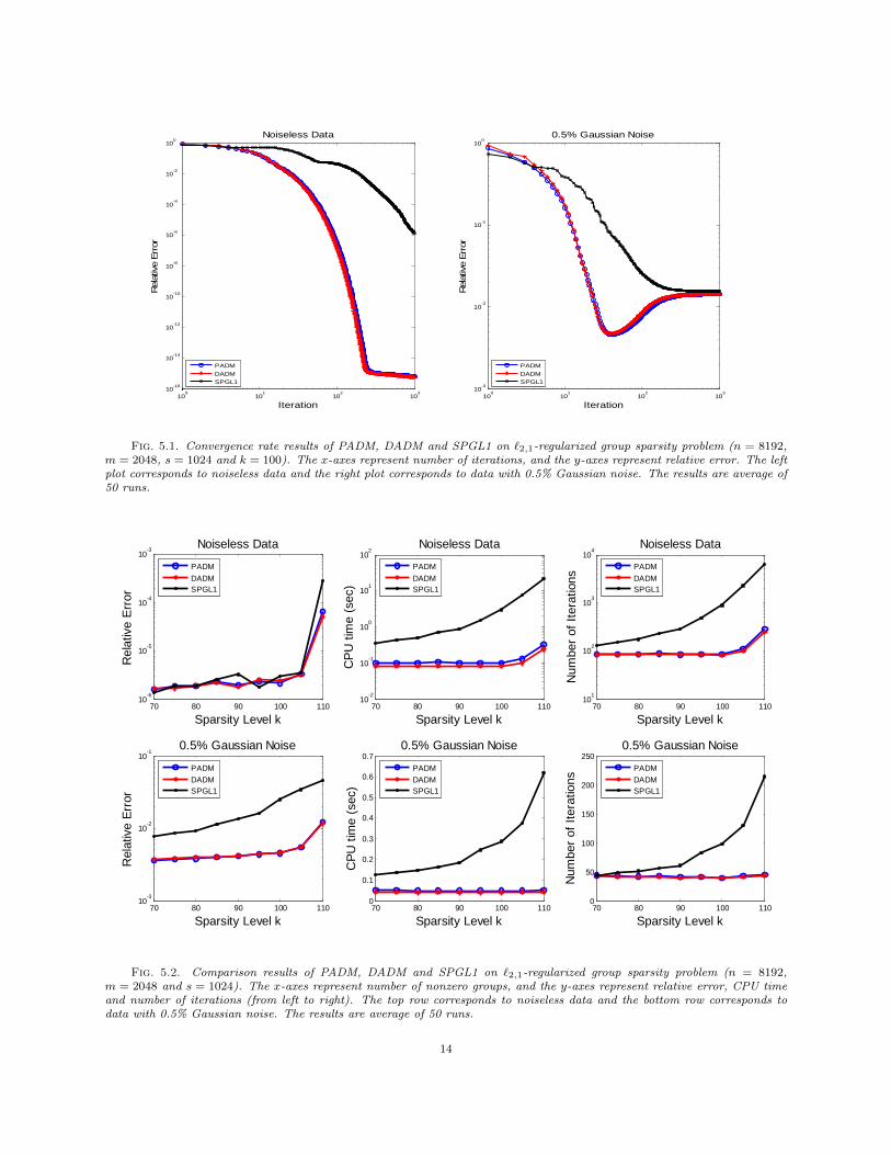
Fig. 5.1. Convergence rate results of PADM, DADM and SPGL1 on `2,1-regularized group sparsity problem (n = 8192,m = 2048, s = 1024 and k = 100). The x-axes represent number of iterations, and the y-axes represent relative error. The leftplot corresponds to noiseless data and the right plot corresponds to data with 0.5% Gaussian noise. The results are average of50 runs.

70 80 90 100 11010

-6

10-5

10-4

10-3

Sparsity Level k

Rel

ativ

e E

rror

Noiseless Data

PADM

DADMSPGL1

70 80 90 100 11010

-2

10-1

100

101

102

Sparsity Level k

CP

U t

ime

(sec

)

Noiseless Data

PADM

DADMSPGL1

70 80 90 100 11010

1

102

103

104

Sparsity Level k

Num

ber

of I

tera

tions

Noiseless Data

PADM

DADMSPGL1

70 80 90 100 11010

-3

10-2

10-1

Sparsity Level k

Rel

ativ

e E

rror

0.5% Gaussian Noise

PADM

DADMSPGL1

70 80 90 100 1100

0.1

0.2

0.3

0.4

0.5

0.6

0.7

Sparsity Level k

CP

U t

ime

(sec

)

0.5% Gaussian Noise

PADM

DADMSPGL1

70 80 90 100 1100

50

100

150

200

250

Sparsity Level k

Num

ber

of I

tera

tions

0.5% Gaussian Noise

PADM

DADMSPGL1

Fig. 5.2. Comparison results of PADM, DADM and SPGL1 on `2,1-regularized group sparsity problem (n = 8192,m = 2048 and s = 1024). The x-axes represent number of nonzero groups, and the y-axes represent relative error, CPU timeand number of iterations (from left to right). The top row corresponds to noiseless data and the bottom row corresponds todata with 0.5% Gaussian noise. The results are average of 50 runs.

14

100

101

102

103

10-16

10-14

10-12

10-10

10-8

10-6

10-4

10-2

100

Iteration

Rel

ativ

e Err

or

Noiseless Data

100

101

102

103

10-3

10-2

10-1

100

Iteration

Rel

ativ

e Err

or

0.5% Gaussian Noise

PADM

DADMSPGL1

PADM

DADMSPGL1

Fig. 5.3. Convergence rate results of PADM, DADM and SPGL1 on `2,1-regularized joint sparsity problem (n = 1024,m = 256, l = 16 and k = 115). The x-axes represent number of iterations and the y-axes represent relative error. The leftplot corresponds to noiseless data and the right plot corresponds to data with 0.5% Gaussian noise. The results are average of50 runs.

100 105 110 115 12010

-3

10-2

10-1

Sparsity Level k

Rel

ativ

e E

rror

0.5% Gaussian Noise

PADM

DADMSPGL1

100 105 110 115 1200

0.2

0.4

0.6

0.8

1

1.2

1.4

Sparsity Level k

CP

U t

ime

(sec

)

0.5% Gaussian Noise

PADM

DADMSPGL1

100 105 110 115 120

50

100

150

200

Sparsity Level k

Num

ber

of I

tera

tions

0.5% Gaussian Noise

PADM

DADMSPGL1

100 105 110 115 12010

-6

10-5

10-4

Sparsity Level k

Rel

ativ

e E

rror

Noiseless Data

PADM

DADMSPGL1

100 105 110 115 12010

-1

100

101

102

Sparsity Level k

CP

U t

ime

(sec

)

Noiseless Data

PADM

DADMSPGL1

100 105 110 115 12010

1

102

103

104

Sparsity Level k

Num

ber

of I

tera

tions

Noiseless Data

PADM

DADMSPGL1

Fig. 5.4. Comparison results of PADM, DADM and SPGL1 on `2,1-regularized joint sparsity problem (n = 1024, m = 256and l = 16). The x-axes represent number of nonzero rows, and the y-axes represent relative error, CPU time and number ofiterations (from left to right). The top row corresponds to noiseless data and the bottom row corresponds to data with 0.5%Gaussian noise. The results are average of 50 runs.

15

5.3. Discussions. As we can see from both Figure 5.1 and Figure 5.3, the relative error curves produced

by PADM and DADM almost coincide and fall quickly below the one by SPGL1 in either noiseless or noisy

case. In other words, the ADM algorithms decrease the relative error much faster than SPGL1. With noiseless

data, the ADM algorithms reach machine precision 10−16 after 200 ∼ 300 iterations, whereas SPGL1 attains

only 10−5 ∼ 10−6 accuracy after 1000 iterations. Although SPGL1 will reach machine precision eventually,

it needs far more iterations.

When the data contains noise, high accuracy is generally not achievable. With 0.5% additive Gaussian

noise, all the algorithms converge to the same relative error level around 10−2. However, we can observe that

the ADM algorithms and SPGL1 have different solution paths. While SPGL1 decreases the relative error

almost monotonically, the relative error curves of the ADM algorithms have a “down-then-up” behavior.

Specifically, their relative error curves first go down quickly and reach the lowest level around 5× 10−3, but

then they start to go up a bit until convergence. This “down-then-up” phenomenon is because the optima of

the `2,1-problem with erroneous data may not necessarily yield the best solution quality. In fact, the ADM

algorithms still keep decreasing the objective values even though the relative errors start to increase. In

other words, the ADM algorithms may give a better solution if it is stopped properly prior to convergence.

We can see that SPGL1 takes approximately 200 iterations to decrease the relative error to 10−2, while the

ADM algorithms need only 30 iterations to reach even higher accuracy.

To further assess the efficiency of the ADM algorithms, we study the comparison results on relative error,

CPU time and number of iterations for different sparsity levels. As can be seen in Figure 5.2 and Figure 5.4,

PADM and DADM have very similar performance though DADM is often slightly faster. They both exhibit

good stability, attaining the desired accuracy with roughly the same number of iterations over different

sparsity levels. Although SPGL1 can also stably reach comparable accuracy, it consumes substantially more

iterations as the sparsity level increases. For noisy data, the ADM algorithms obtain a bit higher accuracy

than SPGL1, which is due to the different solution paths as shown in Figure 5.1 and Figure 5.3. For the

ADM algorithms, recall that the stopping tolerance for relative change is set to 5 × 10−4. Using similar

tolerance values that are consistent with the noise level, the ADM algorithms are often terminated near the

point with the lowest relative error. However, SPGL1 could hardly further lower its relative error by using

different tolerance values.

Moreover, we can observe that the speed advantage of the ADM algorithms over SPGL1 is significant.

Notice that the dominating computational load for all the algorithms are matrix-vector multiplications. For

both PADM and DADM, the number of matrix-vector multiplications are two per iteration. The number

used by SPGL1 may vary in each iteration, usually more than two per iteration on average. Compared to

SPGL1, the ADM algorithms not only consume fewer iterations to obtain the same or even higher accuracy,

but are also less computationally expensive at each iteration. Therefore, the ADM algorithms are much

faster in terms of CPU time, especially as sparsity level increases. For noiseless data, we observe that the

ADM algorithms are 2 ∼ 3 orders of magnitude faster than SPGL1. From Figure 5.1 and Figure 5.3, it is

clear to see that the speed advantage will be even more significant for higher accuracy. For noisy data, the

ADM algorithms gain 3 ∼ 8 times speed up over SPGL1.

16

6. Conclusion. We have proposed efficient alternating direction methods for group sparse optimization

using `2,1-regularization. General group configurations such as overlapping groups and incomplete cover are

allowed. The convergence of these ADM algorithms are guaranteed by the existing theory if one minimizes a

convex quadratic function exactly at each iteration. When the measurement matrix A is a partial transform

matrix that has orthonormal rows, the main computational cost is only two matrix-vector multiplications

per iteration. In addition, such a matrix A can be treated as a linear operator without explicit storage,

which is particularly desirable for large-scale computation. For a general matrix A, solving a linear system is

additionally needed. Alternatively, we may choose to minimize the quadratics approximately, e.g, by taking a

steepest descent step. Empirical evidence has led us to believe that for this latter case, convergence guarantee

should still hold under certain conditions on the step lengths γ1, γ2 (or γ). Our numerical results have

demonstrated the effectiveness of the ADM algorithms for group and joint sparse solution reconstructions.

In particular, our implementations of the ADM algorithms exhibit a clear and significant speed advantage

over the state-of-the-art solver SPGL1. Moreover, it has been observed that at least on random problems

ADM algorithms are capable of achieving a higher solution quality than SPGL1 can when data contains

noise.

Acknowledgments. We would like to thank Dr. Ewout van den Berg for clarifying the parameters

of SPGL1. The work of Wei Deng was supported in part by NSF Grant DMS-0811188 and ONR Grant

N00014-08-1-1101. The work of Wotao Yin was supported in part by NSF career award DMS-07-48839, NSF

ECCS-1028790, ONR Grant N00014-08-1-1101, and an Alfred P. Sloan Research Fellowship. The work of

Yin Zhang was supported in part by NSF Grant DMS-0811188 and ONR Grant N00014-08-1-1101.

REFERENCES

[1] M. Yuan and Y. Lin, “Model selection and estimation in regression with grouped variables,” Journal of the Royal Statistical

Society: Series B (Statistical Methodology), vol. 68, no. 1, pp. 49–67, 2006.

[2] F. Bach, “Consistency of the group Lasso and multiple kernel learning,” The Journal of Machine Learning Research,

vol. 9, pp. 1179–1225, 2008.

[3] S. Ma, X. Song, and J. Huang, “Supervised group Lasso with applications to microarray data analysis,” BMC bioinfor-

matics, vol. 8, no. 1, p. 60, 2007.

[4] D. Eiwen, G. Taubock, F. Hlawatsch, and H. Feichtinger, “Group Sparsity Methods For Compressive Channel Estimation

In Doubly Dispersive Multicarrier Systems,” 2010.

[5] E. van den Berg, M. Schmidt, M. Friedlander, and K. Murphy, “Group sparsity via linear-time projection,” Dept. Comput.

Sci., Univ. British Columbia, Vancouver, BC, Canada, 2008.

[6] J. Liu, S. Ji, and J. Ye, “SLEP: Sparse Learning with Efficient Projections,” Arizona State University, 2009.

[7] Z. Qin, K. Scheinberg, and D. Goldfarb, “Efficient Block-coordinate Descent Algorithms for the Group Lasso,” 2010.

[8] S. Wright, R. Nowak, and M. Figueiredo, “Sparse reconstruction by separable approximation,” Signal Processing, IEEE

Transactions on, vol. 57, no. 7, pp. 2479–2493, 2009.

[9] J. Yang and Y. Zhang, “Alternating Direction Algorithms for `1-Problems in Compressive Sensing,” Arxiv preprint

arXiv:0912.1185, 2009.

[10] Y. Wang, J. Yang, W. Yin, and Y. Zhang, “A new alternating minimization algorithm for total variation image recon-

struction,” SIAM Journal on Imaging Sciences, vol. 1, no. 3, pp. 248–272, 2008.

[11] J. Yang, W. Yin, Y. Zhang, and Y. Wang, “A fast algorithm for edge-preserving variational multichannel image restora-

tion,” SIAM Journal on Imaging Sciences, vol. 2, no. 2, pp. 569–592, 2009.

[12] Y. Zhang, “An Alternating Direction Algorithm for Nonnegative Matrix Factorization,” TR10-03, Rice University, 2010.

17

[13] Z. Wen, W. Yin, and Y. Zhang, “Solving a low-rank factorization model for matrix completion by a nonlinear successive

over-relaxation algorithm,” TR10-07, Rice University, 2010.

[14] Y. Shen, Z. Wen, and Y. Zhang, “Augmented Lagrangian alternating direction method for matrix separation based on

low-rank factorization,” TR11-02, Rice University, 2011.

[15] Y. Xu, W. Yin, Z. Wen, and Y. Zhang, “An Alternating Direction Algorithm for Matrix Completion with Nonnegative

Factors,” Arxiv preprint arXiv:1103.1168, 2011.

[16] R. Glowinski and P. Le Tallec, Augmented Lagrangian and operator-splitting methods in nonlinear mechanics. Society

for Industrial Mathematics, 1989.

[17] R. Glowinski, Numerical methods for nonlinear variational problems. Springer Verlag, 2008.

[18] L. Jacob, G. Obozinski, and J. Vert, “Group Lasso with overlap and graph Lasso,” in Proceedings of the 26th Annual

International Conference on Machine Learning, pp. 433–440, ACM, 2009.

[19] J. Meng, W. Yin, H. Li, E. Hossain, and Z. Han, “Collaborative Spectrum Sensing from Sparse Observations in Cognitive

Radio Networks,” 2010.

[20] D. Baron, M. Wakin, M. Duarte, S. Sarvotham, and R. Baraniuk, “Distributed compressed sensing,” preprint, 2005.

[21] H. Krim and M. Viberg, “Two decades of array signal processing research: the parametric approach,” Signal Processing

Magazine, IEEE, vol. 13, no. 4, pp. 67–94, 2002.

[22] K. Pruessmann, M. Weiger, M. Scheidegger, and P. Boesiger, “SENSE: sensitivity encoding for fast MRI,” Magnetic

Resonance in Medicine, vol. 42, no. 5, pp. 952–962, 1999.

18