growth, development, and technological changeftp.iza.org/dp2558.pdfgrowth, development, and...
TRANSCRIPT

IZA DP No. 2558
Growth, Development, and Technological Change
Volker GrossmannThomas M. Steger
DI
SC
US
SI
ON
PA
PE
R S
ER
IE
S
Forschungsinstitutzur Zukunft der ArbeitInstitute for the Studyof Labor
January 2007

Growth, Development,
and Technological Change
Volker Grossmann University of Fribourg, CESifo and IZA
Thomas M. Steger
ETH Zurich and CESifo
Discussion Paper No. 2558 January 2007
IZA
P.O. Box 7240 53072 Bonn
Germany
Phone: +49-228-3894-0 Fax: +49-228-3894-180
E-mail: [email protected]
Any opinions expressed here are those of the author(s) and not those of the institute. Research disseminated by IZA may include views on policy, but the institute itself takes no institutional policy positions. The Institute for the Study of Labor (IZA) in Bonn is a local and virtual international research center and a place of communication between science, politics and business. IZA is an independent nonprofit company supported by Deutsche Post World Net. The center is associated with the University of Bonn and offers a stimulating research environment through its research networks, research support, and visitors and doctoral programs. IZA engages in (i) original and internationally competitive research in all fields of labor economics, (ii) development of policy concepts, and (iii) dissemination of research results and concepts to the interested public. IZA Discussion Papers often represent preliminary work and are circulated to encourage discussion. Citation of such a paper should account for its provisional character. A revised version may be available directly from the author.

IZA Discussion Paper No. 2558 January 2007
ABSTRACT
Growth, Development, and Technological Change*
The theory of endogenous technical change has deeply contributed to our understanding of the fundamental sources of economic growth and development. In this chapter we survey important contributions in the field by focussing on the basic structure of endogenous growth models with horizontal as well as vertical innovation and emphasizing important implications for growth policy. We address issues like the scale effect problem, directed technological change to understand the evolution of wage inequality, long-run divergence between the innovating North and the imitating South due to inappropriate technology in the South, the relationship between trade and growth, competition and R&D, and the role of imperfect capital markets for R&D-based growth. JEL Classification: O10, O30, O40 Keywords: endogenous technical change, economic growth, horizontal innovations,
scale effects, vertical innovations Corresponding author: Volker Grossmann Department of Economics University of Fribourg Bd. de Pérolles 90 CH-1700 Fribourg Switzerland E-mail: [email protected]
* This chapter is prepared for the UNESCO EOLSS ENCYCLOPEDIA OF MATHEMATICAL SCIENCES/Mathematical Models in Economics.
1 Introduction
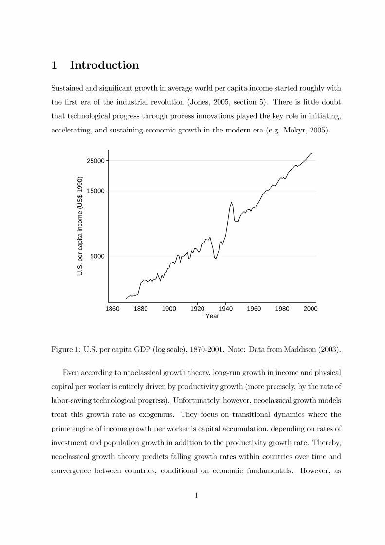
Sustained and significant growth in average world per capita income started roughly with
the first era of the industrial revolution (Jones, 2005, section 5). There is little doubt
that technological progress through process innovations played the key role in initiating,
accelerating, and sustaining economic growth in the modern era (e.g. Mokyr, 2005).
5000
15000
25000
U.S
. per
cap
ita in
com
e (U
S$
1990
)
1860 1880 1900 1920 1940 1960 1980 2000Year
Figure 1: U.S. per capita GDP (log scale), 1870-2001. Note: Data fromMaddison (2003).
Even according to neoclassical growth theory, long-run growth in income and physical
capital per worker is entirely driven by productivity growth (more precisely, by the rate of
labor-saving technological progress). Unfortunately, however, neoclassical growth models
treat this growth rate as exogenous. They focus on transitional dynamics where the
prime engine of income growth per worker is capital accumulation, depending on rates of
investment and population growth in addition to the productivity growth rate. Thereby,
neoclassical growth theory predicts falling growth rates within countries over time and
convergence between countries, conditional on economic fundamentals. However, as
1

shown in Fig. 1, historical evidence points to a relative stability of growth rates for
more than a century in the U.S. Moreover, there is long-run divergence in per capita
income between major regions in the world.1 Fig. 2 illustrates that economic divergence
is not a recent phenomenon but started roughly with the beginning of the modern era,
characterized by relatively fast growth in Western countries and slow growth in Africa
in the last two centuries.
0
5000
10000
15000
20000
25000
Per
cap
ita in
com
e (U
S$
1990
)
1820 1840 1860 1880 1900 1920 1940 1960 1980 2000Year
Western Europe AsiaLatin America Eastern EuropeAfrica Western Offshoots
Figure 2: Divergence in per capita income, 1820-2001. Note: Data from Maddison(2003).
From this brief discussion, it is evident that models which endogenize technological
change are highly desirable to understand the process of economic development in the
long-run. In this survey, we outline in some detail important theoretical approaches in
1By allowing for accumulation of human capital in the basic model of Solow (1956), Mankiw, Romerand Weil (1992) argue that, using data from the period 1960-85, about 80 percent of the cross-countryvariation in income can be explained by focusing on the steady state of the augmented Solow-model,through differences in investment rates and the population growth rate. However, they do not addressthe overwhelming evidence on long-run divergence. Moreover, Bernanke and Gürkaynak (2001) findthat, inconsistent with the Solow-model, the long-run growth rate depends on behavioral variables,particularly on the rate of investment of physical capital.
2

which technological progress is driven by deliberate R&D investments of private agents
in response to market incentives. This literature, starting with Romer (1990), rests on
the basic premise that intentional innovations require resources spent prior to both pro-
duction of goods and product market competition. It thereby abandons the neoclassical
paradigm of perfect competition and constant-returns to scale in the production process,
which (as we point out in more detail in section 2) runs into the fundamental problem
that it leaves no resources for the private sector to finance the search for innovations.
The second premise of endogenous growth theory is that technological knowledge, in the
form of a set of instructions how to produce goods and services (called “idea”, “blue-
print” or “design” in the literature), is a non-rival good; that is, an innovation can be
used by others without diminishing the knowledge of the innovator. This implies that,
without ways to exclude others from (some of) the newly created knowledge, in a large
society no agent would have an incentive to incur any costs to innovate. (At least this
is true when potential innovators are motivated alone by material benefits which ac-
crue from applying the innovation.) An innovation would then be a pure public good,
which suffers from underprovision when privately supplied (with zero provision when
the number of agents goes to infinity). Intellectual property rights protection, which
emerged in Britain already in the seventeenth century, may thus play an important role
for stimulating innovations.2
In sum, endogenous growth theory captures the notion that knowledge accumulates
through the arrival of new ideas which are an outcome of profit-oriented R&D invest-
ments. By outlining basic approaches of this theory we demonstrate that it generates a
wide range of interesting hypotheses and policy implications.
Our survey is structured into three main parts. In section 2, we present models
2The historical role of patents for the growth process is still under debate, however. For instance,Khan and Sokoloff (2001) show that the open patent system in the U.S. stimulated research activity inthe nineteenth century. In contrast, Mokyr (2005) argues that the patent system in Britain did not playa major role in advancing technological knowledge during the first industrial revolution. Rather, non-material benefits like honor and prestige to individual innovators provided important R&D incentives.Moreover, accumulation of knowledge often rested on small and continuous technological improvementswithin firms created by skilled engineers who found productivity-enhancing ways to apply major inven-tions like the steam engine. As it may not be possible to immediately imitate such improvements, thereare incentives to innovate even in absence of intellectual property rights.
3

where growth is driven by new intermediate inputs (“horizontal innovations”), capturing
specialization gains. The section builds on the seminal paper by Romer (1990). One
major issue which has arisen from early models of endogenous technical change is the
prediction of “scale effects” in growth rates, meaning that economies which possess a
larger workforce that is capable to conduct R&D have higher per capita income growth
rates. However, this result is inconsistent with the evidence that the U.S. economy is
characterized by a fairly balanced (at least clearly non-accelerating) long-run growth
path (recall Fig. 1) despite large increases in the number of employed scientists and
engineers during the second half of the twentieth century (Jones, 1995a,b, 2005). We
discuss how Jones (1995a,b) eliminates the prediction of scale effects in growth rates. In
his so-called semi-endogenous growth model, positive long-run growth is possible only
if there is positive population growth. We then turn to three applications of the basic
framework with horizontal innovations. First, following Acemoglu (1998, 2002), we allow
for technological change which is directed to various skill types, thereby addressing the
widely-discussed evidence on rising skill premia in many developed countries, despite
increasing relative supply of skilled labor, in the last few decades. Second, we present
a two-economy (“North” and “South”) model, where economies differ in their relative
endowment of skilled labor. We show that, although the South can imitate the technology
of the innovating North at a small cost, output per worker is larger in the North, due
to different factor endowments (Acemoglu and Zilibotti, 2001). Third, we highlight the
role of horizontal innovations for the impact of liberalization of goods trade on economic
growth (Rivera-Batiz and Romer, 1991). In section 3, we turn to models of “vertical
innovations”, where growth is driven by quality-improvements of intermediate goods. We
first present a version of the “creative destruction” model by Aghion and Howitt (1992).
As many models of endogenous technical change, in addition to scale effects in growth
rates, the model predicts that higher market power is unambiguously conducive to R&D
expenditure. As the scale effects prediction, this result is refuted by empirical evidence
(e.g. Blundell, Griffith and van Reenen, 1999; Aghion, Bloom, Blundell, Griffith and
Howitt, 2005, Aghion, Blundell, Griffith, Howitt and Prantl, 2006). Following Aghion
and Howitt (2005), we therefore present a model with vertical innovations which modifies
4

this result and has interesting implications for industrial R&D policy. In section 4, we
allow for horizontal differentiation in a model of vertical innovations, like in Dinopoulos
and Thompson (1998), Peretto (1998), Segerstrom (1998), Young (1998).3 This class of
models eliminates the scale effect in growth rates like semi-endogenous growth models
but at the same time allows for positive income growth even in absence of population
growth. Finally, we introduce borrowing constraints for financing R&D into this model.
The resulting model suggests an important role of credit market imperfections for long-
run divergence, as recently emphasized by Aghion, Howitt and Mayer-Foulkes (2005).
2 Horizontal Innovation
The models considered in this section explain economic development to result from the
interplay between capital accumulation and endogenous technological change. Private
firms engage in R&D which results in new varieties of intermediate (or capital) goods.4
Since new intermediate goods are of the same quality as previously invented goods,
technological change here takes the form of horizontal innovations.
2.1 The Romer model
2.1.1 The challenge of modelling technological change
The neoclassical growth model relies on exogenous technological progress as the ultimate
engine of long-run economic growth (Solow, 1956; Swan, 1956). Romer (1990) was the
first who formulated an explicit and rigorous growth model with endogenous technical
progress. His analysis is based on three premises: (i) economic growth is driven by
technological progress as well as capital accumulation; (ii) technological progress results
from deliberate actions taken by private agents who respond to market incentives; (iii)
technological knowledge is a non-rivalrous input. We will see below how these premises
are formalized within the model.3For simplicity, we focus on a discrete time version of this class of models, as in Young (1998).4In the Grossman-Helpman (1991, chapter 3) model, not considered here, technological change takes
the form of new varieties of consumer goods.
5

Formulating a general equilibrium model with endogenous technological change, as
required by premise (ii) above, is all but trivial.5 The major theoretical difficulty can be
sketched as follows. Consider an economy producing a final output good Y according to
the production technology Y = F (A,K,L), where A denotes the state of technology, K
the stock of physical capital, L labor input, and F (.) is C2 with ∂F (.)∂X
> 0 and ∂2F (.)∂X2 < 0
for all X ∈ {A,K,L}. It is further assumed that F (.) exhibits constant returns to
scale (CRS) in capital and labor, i.e. λY = F (A, λK, λL) for any λ ≥ 0. Neoclassical
theory relies on perfect competition such that all factors are rewarded according to
their marginal product. This in turn implies that output is completely exhausted, i.e.
Y = FK(.)K + FL(.)L with FK(.) :=∂F (.)∂K
denoting the marginal product of capital etc.
Now it becomes obvious that any theory which rests on perfect competition together
with CRS and should fulfill premise (ii) runs into a fundamental problem. Those agents
who bring technical change about are assumed to react to market incentives and must
therefore be rewarded somehow. Since output is, however, completely used up by paying
wages to labor and rental prices to capital owners, nothing is left to reward researchers.
2.1.2 The structure of the model
We consider a simplified version of the Romer (1990) model in that there is only one
type of labor.6 The household side is identical to the Ramsey model of optimal growth
(see, for instance, Barro and Sala-i-Martin, 2004, chapter 2). On the production side
there are three sectors: a final output sector, a producer durables sector, and a research
sector.
Households. The economy is populated by a continuum of mass one identical
households. Each household is endowed with L units of labor services per unit of time,
which are inelastically supplied (independent of the wage rate) to the market. Households
are assumed to choose the time path of consumption C(t) so as to maximize the present
discounted value of an infinite utility streamR∞0
C(t)1−σ−11−σ e−ρtdt, where σ > 0 and ρ > 0 is
5Earlier contributions modelled technical progress as a by-product of capital accumulation (Arrow,1962; Romer, 1986).
6Romer (1990) distinguishes between unskilled labor and skilled labor (human capital). This dis-tinction is, however, not essential for the derived results; it merely relabels the relevant scale variable,as explained below.
6

the time preference rate. The optimal consumption path obeys the well-known Keynes-
Ramsey rule (KRR)C(t)
C(t)=
r(t)− ρ
σ, (1)
where C(t) := dC(t)/dt denotes the rate of change of consumption and r(t) is the interest
rate in t.
Final output sector. Firms in the final output sector produce a homogenous good
Y that can be either consumed or used as an input in the production of differentiated
capital goods. The market for the final output good is perfectly competitive. The
technology is given by7
Y = L1−αY
Z A
0
x(i)αdi, (2)
where LY is the amount of labor devoted to Y -production, x(i) is the amount of capital
good i ∈ [0, A], and 0 < α < 1. In equilibrium x(i) = x for all i and hence the above
technology can be expressed as Y = L1−αY Axα. Moreover, if we define aggregate capital
as K := Ax, one may write
Y = (ALY )1−αKα. (3)
This formulation shows that equ. (2) boils down to a Cobb-Douglas technology with
labor-augmenting technical change and hence makes an important implication obvious:
Even if one holds the total amount of capital K = Ax constant, an increase in the
"number" of varieties A boosts the productivity of labor. Hence, technology (2) captures
the basic idea that specialization, as reflected by an increasing number of intermediate
goods x(i), makes the production process more and more efficient (Smith, 1776, Book I,
chapter I; Ethier, 1982; Solow, 2000, chapter 9). Final output is chosen as the numeraire,
its price is set equal to unity pY = 1.
Producer durables sector. Producers in this sector manufacture differentiated
capital goods x(i), also labelled "producer durables" or simply "machines". As a techni-
cal and legal prerequisite for production, firms must at first purchase a blueprint (design).
Technology (2) implies that the x(i) are imperfect substitutes in Y -production; this as-
7The time index t is often supressed to simplify the notation.
7
sumption is crucial for monopolistic competition in the market for producer durables.8
As regards the production technology for x(i), it is assumed that it takes one unit of
"raw capital" (output not consumed) to create one unit of any type of durables (Romer,
1990, p. S82).9 The constant marginal production cost of x therefore equals the interest
rate r. As regards the institutional structure, it is assumed that x-producers rent their
machines to Y -producers by charging a rental price.
R&D sector. Firms in the research sector search for new and economically valuable
ideas. An "idea" is a blueprint (design) for a new producer durable. The market for
designs is perfectly competitive and characterized by free entry.10 R&D is modelled as
a deterministic process. The R&D technology is given by
A = ηALA, (4)
where A := dA/dt denotes the rate of change in the number of blueprints A per period
of time dt, LA the amount of labor devoted to R&D, and η > 0. Notice that the
productivity of researchers LA increases with technological knowledge A; see premise
(iii) above.11
It should be noted that there is a double knife-edge restriction implicit in this for-
mulation: (i) ∂ ln A∂ lnA
= 1 and (ii) ∂ ln A∂ lnLA
= 1. The first is needed for sustained growth
to be feasible.12 The second is required for a consistent microeconomic structure, i.e.
a perfectly competitive market requires CRS in the single private input LA. It is fur-
ther assumed that, once a new idea is found, its producer obtains perfect and perpetual
patent protection.
Equilibrium in the labor market requires L = LA + LY . Equilibrium in the capital
market requires that the household’s financial capital equals the total physical capital
8The elasticity of substitution between any two x(i) is 1 < 11−α <∞.
9This modelling assumption is further explained in Rivera-Batitz and Romer (1991, p. 534): "Thisdoes not mean that consumption goods are directly converted into capital goods. Rather, the inputsneeded to produce one unit of consumption are shifted from the production of consumption goods intothe production of capital goods."10In the words of Romer (1990, p. S85) "anyone engaged in research can freely take advantage of the
entire existing stock of designs in doing research to produce new designs".11Acemoglu (2002, p. 793) uses the phrase "current researchers ‘stand on the sholder of giants‘."12For a critical discussion of this linearity assumption see Solow (2000, chapter 9).
8

employed by final output firms K.
The long run growth rate. The final output technology (3) indicates that, along
the balanced growth path (BGP), this model is equivalent to a neoclassical growth model
with labor-augmenting technical progress. This implies that the following relations must
hold along the BGP: Y = K = C = A = g, where X := X/X for all X ∈ {Y,K,C,A}.
Moreover, the R&D technology (4) implies that the long run growth rate of A is
A = ηL∗A,
where L∗A denotes the constant amount of labor devoted to R&D. The economically
interesting question then concerns the determination of L∗A. This is the issue we consider
at next.
2.1.3 The decentralized solution
To determine the long run growth rate of the market economy we start with the equilib-
rium condition stating that the wage rate of labor employed in Y -production (wY ) must
equal the wage rate of labor employed in R&D (wR&D). The competitive wage rates in
both sectors equal the respective value marginal product of labor. From (2) and (4) one
therefore gets
wY = (1− α)L−αY Axα
wR&D = pAηA,
where pA is the price of a blueprint. Operating profits of the typical x-producer are
π = (pD(x) − r)x with pD(x) denoting the demand price (or inverse demand function)
of x, which is given by
pD(x) = αL1−αY xα−1. (5)
The typical x-producer faces constant marginal cost, equal to r, and a constant
elasticity demand curve with a price elasticity equal to 1α−1 < −1. It is well known
that, in this case, the optimal supply price is a mark-up over marginal cost according to
pS =rα. Moreover, using r = αpS we have π = (pD − αpS)x. From equilibrium in the
9

x-market, pD = pS = p, and plugging (5) into the profit function one gets
π = (1− α)px = (1− α)αL1−αY xα.
Assuming that the economy grows along a BGP, which implies that both π and r
are constant, the price of a blueprint may be expressed as pA = πr. Hence, the price
of a blueprint may be written as pA =(1−α)αL1−αY xα
r. Now evaluating the equilibrium
condition wY = wR&D yields13
(1− α)L−αY Axα =ηA(1− α)αL1−αY xα
r,
which immediately gives r = ηαLY . Plugging LY = L− LA (labor market equilibrium)
and LA = gη(from (4)) into the preceding equation leads to a condition describing
equilibrium on the supply side of the economy
r = ηαL− αg. (6)
The economic reason for the negative relationship between r and g is that an increase in
r lowers pA = πrand therefore R&D firms employ a lower amount of labor. Equilibrium
on the demand side is described by the KRR, equ. (1), which may be expressed as
r = σg + ρ. (7)
The positive association between r and g captures the fact that an increase in r motivates
households to save more which boost growth. Solving (6) and (7) for g yields g = ηαL−ρσ+α
.14
Since growth cannot become negative in this model, the long run growth rate of the
13This condition can be expressed as πr =
wηA and hence is equivalent to the free entry condition
(implying zero profits) in the R&D sector. To see this, note that under (4), profits are given byPAηALA − wLA and use PA = π
r .14One can equivalently solve (6) and (7) for r and then evaluate r = ηα(L − LA), which gives L∗A.
Plugging the result into g = A = ηAL∗A yields, of course, the same solution.
10

market economy, denoted gM , reads
gM =
⎧⎨⎩ ηαL−ρσ+α
for ηαL > ρ
0 for ηαL ≤ ρ. (8)
Long run growth obviously requires that the economy is large enough in the sense that
ηαL > ρ. Moreover, the preceding solution shows a scale effect since, provided that
ηαL > ρ, larger economies (with size being measured by L) do grow at a higher rate.
The economic reason for this scale effect implication is that, along the BGP, a constant
fraction of the labor force is devoted to R&D. More researchers produce more knowl-
edge, which in turn improves the productivity of the R&D sector such that long run
growth accelerates. This effect does, however, depend critically on the strength of the
intertemporal knowledge spill-over, as will be discussed below.
2.1.4 Market imperfections and policy implications
So far we have focused on the decentralized economy. Turning to the social planner’s
solution, it can be readily shown that the optimal long run growth rate, gS, is given by
(Chiang, 1992)
gS =
⎧⎨⎩ηL−ρσ
for ηL > ρ
0 for ηL ≤ ρ. (9)
Comparing this result to (8) shows that gM < gS. The market economy grows at a
pace which is too low compared to the social optimum. This is due to two imperfections
inherent in the market economy, which bias the private allocation decisions (Jones and
Williams, 2000; Steger, 2005): First, the R&D technology (4) exhibits an intertempo-
ral knowledge spill-over since the productivity of current researcher LA increases with
the stock of knowledge, as measured by A, which has been accumulated in the past.
This social benefit is not reflected in the market price for designs pA = πrand, conse-
quently, R&D incentives are too low. Second, the typical producer durable firm realizes a
monopoly profit by selling a differentiated capital good. It cannot, however, appropriate
the entire "consumer surplus". The gain to society resulting from a new innovation is
11

larger than the private profits earned by the monopolist. This static distortion leads
once more to a price of blueprints which falls short of its social value. Hence, the Romer
(1990) model unambiguously exhibits underinvestment in R&D.15 This basic implication
is in line with empirical studies on the gap between the private and the social rate of
return on R&D. Griliches (1991) reviews this literature and reports social rates of return
of about 40 to 60 percent, which are much higher than private rates of return.
What are appropriate public policies to correct these market failures? One possible
scheme of public policies is as follows. The positive knowledge spill-over can be neu-
tralized by a subsidy on the sales of blueprints. The "consumer surplus" effect can be
corrected by subsidizing the sales of producer durables (Steger, 2005, section II).
2.2 Semi-endogenous R&D-based models
Jones (1995a,b, 2002) has argued that the scale effect implication inherent in the first
generation of R&D-based growth models (Romer, 1990; Grossman and Helpman, 1991,
chapter 3; Aghion and Howitt, 1992) is empirically problematic. Using time series evi-
dence for the G5-group of industrialized economies he shows that the number of scientists
and engineers has risen drastically during the post-WWII period. Even the relation of
scientists and engineers to the total number of employees has increased in the G5-group
as a whole. During the same time period, however, the growth rate of GDP per capita
as well as the TFP growth rate was roughly stationary, or at least non-increasing, in the
U.S. (cf. Figure 1 above) and in the G5 group (see also Jones, 2005, section 5).16
This empirical pattern is clearly at odds with the basic R&D-based growth model
described above. Jones (1995a,b) has accordingly modified the Romer (1990) model to
eliminate the scale effect. Another major result of this line of research is the finding of15There are other R&D-based growth models with positive and negative R&D externalities such that
the amount of resources devoted to R&D might be too high in the market equilibrium (Jones andWilliams, 2000; Steger, 2005; Strulik, 2005). Also horizontal innovation models do not capture anotherimportant externality associated with private R&D, namely the business stealing effect (see Section 3of this article).16The evidence on the scale effect is mixed, however. Kremer (1993) argues that there is a positive
scale effect at the level of the world when considering the very long run (one million B.C. until present).Backus et al. (1992) find mixed results within a cross-sectional studies using different measures for thescale of an economy (e.g. aggregate GDP; manufacturing output; number of scientists, engineers andtechnicians; R&D expenditure).
12

policy ineffectiveness. Public policy is unable to control the long run growth rate. For
this reason Jones used the phrase "semi-endogenous growth model".
The Jones (1995a,b) model is basically identical to the Romer (1990) with one impor-
tant modification. The double knife-edge restriction ∂ ln A∂ lnA
= 1 and ∂ ln A∂ lnLA
= 1 inherent
in the R&D technology, see (4) above, is relaxed by postulating the following (sectoral)
R&D technology
A = ηAφLγA, (10)
where 0 < φ < 1, 0 < γ ≤ 1.17 The total amount of labor is assumed to grow exponen-
tially, i.e. L(t) = L0ent, where n denotes the growth rate of the labor force, and L0 > 0.
As before, along a BGP we have y = k = c = A = g, where small letters denote per
capita quantities.
The determination of the long run growth rate is very simple in this model. Divide
both sides of equ. (10) by A, and use LA =LALL, to get
A =A
A= ηAφ−1(
LA
L)γLγ.
Taking logarithms on both sides yields
Log(A) = Log(η) + (φ− 1)Log(A) + γLog(LA
L) + γLog(L).
Forming the time derivative and noting that (i) A = const. and LAL= const. along a
BGP by definition and (ii) dLog(A)dt
= A etc. one gets
A =γn
1− φ.
The scale effect has obviously been removed from the model. Instead, the growth rate
of per capita income g = y = A is now proportional to the growth rate of the labor force
n. Here we have an important implication for a number of industrialized economies
17Notice that γ < 1 implies decreasing returns to labor at the sectoral level. This formulation iscompatible with CRS at the level of the firm and hence with perfect competition in the R&D sectorin the presence of negative duplication externalities (i.e. the possibility that decentralized R&D mightlead to redundancy).
13

which experience a decline in n. Growth is semi-endogenous: On the one hand, it is
endogenous because growth still results from deliberate actions taken by private agents
who respond to market incentives. On the other hand, it is exogenous to the extent that
public policy cannot control the balanced growth rate.18 In fact, the long run growth
rate is proportional to the growth rate of labor with the factor of proportionality γ1−φ
being determined by the characteristics of the R&D technology.19
Finally it should be noted that Eicher and Turnovsky (1999) have formulated a
more general semi-endogenous R&D-based growth model (which they label non-scale
growth model), showing that the long run growth rate is in general determined by the
characteristics of both the R&D technology and the final output technology.
2.3 Directed technical change
The R&D-based endogenous growth models considered so far are characterized by a
single R&D process. There are, however, a number of important topics (like biased tech-
nological change and the evolution of wage inequality or the consequences of international
trade on the direction of technological change), which require a setup with multiple R&D
processes such that technological change can be directed at different factors of produc-
tion. Hence, we next turn to a model with two sectors, two production factors and two
R&D processes to study the direction of technical change. This approach is due to Ace-
moglu (1998, 2002); see also Gancia and Zilibotti (2005). The model considered here is
a direct extension of the Romer (1990) model.
2.3.1 The basic model setup
Final output sector. There is a large number of mass one of identical firms who
produce a homogenous final output Y under perfect competition using the following
18The long run growth rate of the market economy and the socially controlled economy coincide. Inthis sense there is simply no need for public policy to intervene. Nonetheless, along the BGP, the marketeconomy grows at a lower level compared to the socially controlled economy.19Neither do preferences nor the parameters of final output technology play any role. These parameters
do nonetheless affect the level of the BGP.
14

constant elasticity of substitution (CES) technology
Y =³γY
ε−1ε
L + (1− γ)Yε−1ε
H
´ εε−1,
where YL and YH are intermediate inputs, 0 < γ < 1 is a constant parameter, and
0 < ε < ∞ determines the degree of substitution between YL and YH in Y -production
(as explained below). The final output good can be used for consumption (C), as an
input in the production of machines (I), or as an input in R&D (R). The economy’s
resource constraint accordingly reads Y ≤ C + I +R.
Intermediate goods sector. There is a large number of mass one of identical YL-
producers and a large number of mass one of identical YH-producers. Production takes
place under perfect competition. The production technologies for the two intermediate
goods YL and YH are given by
YL = L1−αZ AL
0
xL(i)αdi (11)
YH = H1−αZ AH
0
xH(i)αdi, (12)
where L denotes unskilled labor, H skilled labor, and 0 < α < 1 a constant parameter.
Notice that the production of YL is assumed to be labor intensive, whereas the production
of YH is human capital intensive. There are two type of producer durables ("machines"),
namely xL(i) with i ∈ [0, AL] and xH(i) with i ∈ [0, AH ]. Machines of type xL(i)
are combined with labor in YL-production, whereas machines xH(i) are combined with
human capital in YH-production. This formulation captures the basic idea that different
input factors (L and H) are combined with different machines and, hence, technological
progress (the introduction of new machines) might favor one factor more than others.
For instance, the introduction of the assembly line primarily increased the productivity
of unskilled labor, whereas the introduction of computers favored human capital.
As before, technical change enhances the spectrum of available machines. The im-
portant point to notice is that the range of machines that can be used with labor is AL,
whereas the range of machines that can be used with human capital is AH . Therefore,
15

in this setup, technical change is either directed at labor (i.e. increasing AL) or directed
at human capital (i.e. enhancing AH).
Machines sector. Firms in this sector conduct R&D and once a firm has found
a blueprint for a new machine it starts production and marketing. There is a large
number of potential suppliers and free entry into this sector. Once a design for a new
machine is found, the successful firm is granted perfect and infinite patent protection
and thereby becomes a "technology monopolist". The market for machines hence is
monopolistically competitive. Machines (xL and xH) are rented to intermediate goods
producers by charging a rental price (pxL, pxH). For simplicity, it is assumed that all
machines depreciate fully after use.20 The marginal production cost is the same for all
machines and equal to ψ in terms of the final good. The R&D technologies are given by
AL = ηLRL
AH = ηHRH ,
where ηL, ηH > 0 and RL is spending on R&D (in terms of final output) for new xL-
machines and RH is spending on R&D for xH-machines. This specification, labelled as
lab-equipment approach, departs from the original Romer model in that final output is
used instead of labor as an input in R&D.
2.3.2 Equilibrium
The typical Y -producer takes the output price pY and input prices (pL and pH) as given.
Profit maximization then implies that an optimal production plan is characterized by
pHpL=1− γ
γ
µYHYL
¶− 1ε
, (13)
i.e. the ratio of input prices (LHS of (13)) must equal the marginal rate of substitution
(RHS of (13)). Here one recognizes that the elasticity of substitution between YH and
20Hence, the machines xL(i) and xH(i) are similar to intermediate goods which are used up in theproduction process. Notice that the original Romer (1990) assumes the opposite polar case of nodepreciation.
16

YL is∂ ln(YH/YL)∂ ln(pH/pL)
= −ε. The final output good Y is chosen as the numeraire and hence
we set21
pY =¡γεp1−εL + (1− γ)εp1−εH
¢ 11−ε = 1. (14)
The producers of intermediate goods (YL and YH) maximize profits
pLYL − wLL−Z AL
0
xL(i)pxL(i)di
pHYH − wHH −Z AH
0
xH(i)pxH (i)di,
taking output prices (pL and pH) and input prices ( pxL, pxH , wL,wH) as given. Noting
(11) and (12) this yields the following demand curves for machines
xL(i) =
µαpLpDxL(i)
¶ 11−α
L (15)
xH(i) =
µαpHpDxH (i)
¶ 11−α
H, (16)
where pDxL(i) and pDxH(i) denote demand prices. Intermediate goods producer accordingly
rent more machines, the higher product prices (pL and pH), the larger the amount of
complementary factors employed (L and H) and the lower the rental price of machines
(pDxL, pDxH). Operating profits of the typical technology monopolists are given by
πL = (pSxL− ψ)xL = (
ψ
α− ψ)
µα2
ψ
¶ 11−α
p1
1−αL L (17)
πH = (pSxH− ψ)xH = (
ψ
α− ψ)
µα2
ψ
¶ 11−α
p1
1−αH H, (18)
where the second equalities follow from the demand curves (15) and (16), noting that the
optimal supply price is a mark up over marginal cost according to pSxL =ψαand pSxH =
ψα,
and using pSxL = pDxL and pSxL = pDxL (equilibrium in the machine markets). The relative
21See Solow (2000, chapter 10) on the determination and interpretation of the CES price index in theDixit-Stiglitz framework.
17

profitability of R&D directed at human capital H and labor L can hence be expressed
asπHπL
=
µpHpL
¶ 11−α H
L. (19)
The incentive to engage in AH-expanding R&D relative to the incentive to conduct
AL-enhancing R&D comprises two components. The first term gives the price effect:
there is a greater incentive to develop technologies producing more expensive goods.
The second term is the market size effect: the incentive to develop a new technology is
proportional to the number of workers that will be using it.
We now turn to the ratio of AH and AL along the BGP. For AH/AL to be constant,
as required for balanced growth, there must be innovating firms in both machine sectors.
This requires that it is equally profitable to invest in AH-expanding and AL-expanding
R&D, i.e. ηHπH = ηLπL. From this condition the constant ratio of technologies can be
shown to read as follows (for details see the appendix)
AH
AL=
µ1− γ
γ
¶εµηHηL
¶θ µH
L
¶θ−1, (20)
where θ := 1+ (ε− 1)(1−α) is the (derived) elasticity of substitution between H and L
(as will become clear below).22 As long as human capital and labor are strong substitutes
(θ > 1), an increase in the supply of one factor will induce more innovation directed to
that specific factor. The reason is that, as long as θ > 1, the market size effect dominates
the price effect. As a consequence, technological change is biased towards the abundant
factor. The reverse holds true for θ < 1. In this case, the price effect dominates the
market size effect and technological change favors the scarce factor.
By determining the equilibrium interest rate from the condition that profits in the
machines sector equal zero and plugging the result into the KRR, the long run growth
rate can be shown to read (for details see the appendix)
g =1
σ(r − ρ) (21)
22Notice that θ > (<)1 requires ε > (<)1.
18

with r := ω³γε (ηLL)
θ−1 + (1− γ)ε (ηHH)θ−1´ 1
θ−1(22)
where ω := (ψα− ψ)
³α2
ψ
´ 11−α. As usual, long run growth decreases with the time pref-
erence rate ρ. It increases with the intertemporal elasticity of substitution 1σand the
interest rate r. The interesting point to notice here is that the interest rate (hence the
growth rate) is determined by the characteristics of all production technologies (final
output, machines, and R&D) as well as by factor endowments (H and L).23
To see the implications of directed technological change for factor prices, one can solve
for wH and wL taking technology (AH and AL) as given (for details see the appendix)
wH
wL=
µ1− γ
γ
¶ εθµAH
AL
¶ θ−1θµH
L
¶− 1θ
. (23)
This relation shows that the (short run) elasticity of substitution between H and L
is ∂ ln(H/L)∂ ln(wH/wL)
= −θ. The relative factor reward is decreasing in the relative factor supply.
This is due to the usual substitution effect. Moreover, when θ > 1 a greater skill bias in
technology AH/AL increases relative factor rewards and vice versa.
We finally look at the implications for relative factor prices in the long run, i.e. when
technology is considered as being endogenous. Inserting (20) into (23) gives a reduced
form solution for the relative factor price
wH
wL=
µηHηL
¶θ−1µ1− γ
γ
¶εµH
L
¶θ−2. (24)
This equation shows that, as long as θ > 2, an increase in relative supply of skilled
labor can go hand in hand with an increase in the skill premium (wHwL). This is due
to endogenous biased technological change towards the more abundant factor since the
market size effect is sufficiently strong. Hence, as argued by Acemoglu (1998), this
model provides a potential explanation for the empirical observation of a rise in the skill
premium in the U.S. during the period 1960-90 despite an increase in the relative supply
of skilled labor.24
23Hence this model also features a scale effect.24For a comprehensive discussion of "technical change and labor market inequalities" see Hornstein,
19

2.4 Appropriate technology and development
The previous section has demonstrated that the directed-technical-change approach can
be used to understand the evolution of wage inequality within an economy. This ap-
proach can also be employed to understand the fundamental causes of the sustained
income gap between industrialized and less developed countries.25 An important reason
for sustained underdevelopment is due to "inappropriate technologies". The model de-
veloped by Acemoglu and Zilibotti (2001) assumes that, quite realistically, less developed
economies imitate the technologies developed in industrialized countries. Provided that
intellectual property rights cannot be enforced in underdeveloped economies, technolo-
gies are designed according to the fundamentals of the rich industrialized countries and
therefore are not optimal when applied in poor underdeveloped economies.
2.4.1 The basic model setup
There are two sets of economies, the North and the South. The North is innovative, as
in the previous sections. The South does not innovate but adopts technologies innovated
in the North. Intellectual property rights cannot be enforced in the South. There is no
trade between the North and the South. The model is similar to the directed technical
change model. There are three sectors, namely a final output sector, an intermediate
goods sector, and a machines sector.
Final output sector. This sector is perfectly competitive. Firms assemble a range
of intermediate goods y(i) with i ∈ [0, 1] to produce final output Y according to
Y = exp
∙Z 1
0
ln y(i)di
¸. (25)
This somewhat unusual production function can be viewed as a symmetric Cobb-Douglas
function. Final output can be used for consumption (C), investment (I), or as an input
in R&D (X). The resource constraint therefore is Y ≤ C+I+X. Moreover, final output
good is chosen as the numeraire good such that pY = 1.
Krusell and Violante (2005).25Caselli (2005) reviews the development accounting literature, which aims at explaining the empirical
causes for international differences in per capita incomes.
20

Intermediate goods sector. There is a continuum of heterogenous sectors produc-
ing intermediate goods y(i). Each intermediate good y(i) can be produced with unskilled
labor l, skilled labor h, and machines. However, each sector has a different production
technology. The key assumption is that some machines can only be used with unskilled
labor, while some other machines can only be used with skilled labor. More specifically,
the production technology for good y(i) is of the following form
y(i) = [(1− i)l(i)]1−αZ AL
0
xαL(i, γ)dγ + [ih(i)]1−α
Z AH
0
xαH(i, ν)dν, (26)
where l(i) and h(i) are the quantities of unskilled and skilled labor employed in sector
i, xL(i, γ) is the quantity of xL-machines of type γ ∈ [0, AL] employed in sector i, and
xH(i, ν) is the quantity of xH-machines of type ν ∈ [0, AH ] in sector i, respectively. Notice
the term (1− i), associated with unskilled labor l(i), and the term i, attached to skilled
labor h(i), which denote exogenous technology-specific and sector-specific productivities.
In sectors with a high i ∈ [0, 1] unskilled labor (which can only be combined with xL-
machines) has a low productivity but skilled labor (which can only be combined with
xH-machines) has a high productivity, and vice versa.
Machines sector. Firms in this sector either innovate (in the North) or imitate
(in the South). Successful innovators in the North are granted perfect patent protection
in the Northern market. Once a blueprint has been invented or copied, firms start to
manufacture and market differentiated machines as technology monopolists. There is a
large number of potential entrants and there is free entry. For reasons which become
clear below, the unit production cost are normalized to α2.
2.4.2 Equilibrium
The North. Each firm in the intermediate goods sector maximizes profits taking the
output price p(i) and input prices (wL, wH , pxL, pxH ) as given. The resulting sectoral
demand curves for xL-machines and xH-machines are as follows (due to symmetry the
21

indices γ and ν can be omitted)
xL(i) = (1− i)l(i)
µαp(i)
pDxL
¶ 11−α
(27)
xH(i) = ih(i)
µαp(i)
pDxH
¶ 11−α
. (28)
Since marginal cost of machine production are equal to α2, the optimal supply price
is pSxL = pSxH = α. Setting pDxL = pSxL = α and pDxH = pSxH = α in (27) and (28) and using
(26) yields an indirect production function for intermediate goods
y(i) = p(i)α
1−α [AL(1− i)l(i) +AHih(i)] . (29)
This formulation shows very clearly that, given AL and AH , the productivity of
unskilled labor decreases with the sector index i, whereas the productivity of skilled
labor increases with the sector index. This implies that there is a critical threshold
J ∈ [0, 1] such that all sectors i ≤ J will employ unskilled labor only (together with
xL-machines), whereas all sectors i > J will employ skilled labor only (together with
xH-machines).
The total profit earned by the typical xL-monopolist is given by πL = (pSxL −
α2)R 10xL(i)di; for xH-monopolist we have πH = (pSxH − α2)
R 10xH(i)di. Noting (27)
and (28) together with pDxL = pSxL = α and pDxH = pSxH = α equilibrium profits read as
follows
πL = (1− α)α
Z 1
0
p(i)1
1−α (1− i)l(i)di (30)
πH = (1− α)α
Z 1
0
p(i)1
1−α ih(i)di. (31)
The prices of intermediate goods are given by (see the appendix for details)
p(i) = p(0)(1− i)−(1−α) ∀ 0 ≤ i ≤ J (32)
p(i) = p(1)i−(1−α) ∀ J < i ≤ 1 (33)
22
where p(0) is the price of y(0) and p(1) is the price of y(1). The economic intuition behind
these price equations is straightforward. Consider the price of intermediate goods, which
are produced with unskilled labor, as given by (32). As i ∈ [0, J ] increases, intermediate
goods y(i) become more expensive since the productivity of unskilled labor l(i) falls with
i. An analogous interpretation applies to p(i) with i ∈ [J, 1], as given by (33).
As has been indicated above, the pattern of sectoral productivities of skilled and
unskilled labor implies that there are two groups of sectors in equilibrium. The first
group produces with unskilled labor and xL-machines, whereas the second employs skilled
labor together with xH-machines. The critical threshold J can be determined from the
condition p(0)(1−J)−(1−α) = p(1)J−(1−α) stating that both sectors are equally profitable
(for the derivation see the appendix):
J =
Ã1 +
µAH
AL
H
L
¶1/2!−1. (34)
Remember that the range of sectors employing unskilled labor is [0, J ]. This range is
accordingly smaller, the higher the skill bias of technology AHALand the larger the relative
human capital endowment HL. The reverse holds true for the range of sectors producing
with unskilled labor, as given by [J, 1].
It can be shown that aggregate output, defined by Y =R 10p(i)y(i)di, is described
by a CES technology in the primary input factors L and H (for the derivation see the
appendix):
Y = exp(−1)h(ALL)
1/2 + (AHH)1/2i2. (35)
Notice that the (derived) elasticity of substitution between L and H in Y -production is
equal to 2.
To complete the description of the macroeconomic equilibrium, we finally report the
skill bias. In the appendix it is shown that along the BGP the skill bias in the North,
with endowments HN and LN of skilled and unskilled labor, respectively, is given by
AH
AL=
HN
LN. (36)
23

This equation shows that the technological skill bias AH
ALis positively associated with the
relative skill endowment HN
LN. This is in fact a special case of the preceding result; see
equ. (20), assuming that θ = 2. Combining (34) and (36), we find that the threshold
sector in the North, JN , is given by JN =³1 + HN
LN
´−1.
The South. The Southern economies are largely identical to the Northern economies.
There are, however, two important exceptions. First, intellectual property rights cannot
be enforced in the South and hence there is no R&D in the South. Machine producers
in the South can copy the blueprints invented in the North at a small fixed cost. As
a result, the South operates with the range of machines as provided by the North,
i.e. [0, AL] and [0, AH ]. Second, the South has a lower relative skill endowment, i.e.HS
LS< HN
LN. From (34) and (36), this implies that the threshold sector in the South
JS = J =
µ1 +
³HN
LN
HS
LS
´1/2¶−1> JN .
2.4.3 Productivity differences
The model set up above implies that output per worker ( YL+H
) in the typical Southern
economy is smaller than output per worker in the typical Northern economy. This re-
sult holds true despite the fact that both group of economies have access to the same
technology. The economic intuition is straightforward: Southern economies use a tech-
nology mix, as given by [0, AL] and [0, AH ], which has been designed according to the
fundamentals of the North, but is suboptimal when applied in the South.
To illustrate the implied productivity differences consider output per worker, which
can be expressed as follows (see equ. (35))
Y
L+H= exp(−1)
h(AL)
1/2 +¡AH
HL
¢1/2i21 +H/L
.
Figure 3 shows that output per worker is an inverse U-shaped function of HL. More-
over, it is easy to show that this curve has a maximum at HL= AH
AL. Considering equ. (36)
shows that this condition holds true for Northern economies. Hence, the technology mixAH
ALis such that labor productivity is indeed maximized in the North. Since Southern
24

economies have a lower relative skill endowment, output per worker in the South falls
short of output per worker in the North.
Figure 3: Output per worker as a function of relative human capital.
The reason for the productivity difference between the North and the South is a
technology-skill mismatch. The North develops technologies that are most appropriate
for its own needs. More specifically, the North develops more skill-biased technologies be-
cause there are relatively more skilled workers using these technologies. These Northern
technologies are mismatched to the skills of the workforce in less developed economies.
This can be seen more clearly from (36), which implies AH(1−JN) = ALJN . Considering
the production function (29) immediately shows that the preceding condition states that
the physical productivities of both skilled and unskilled labor are equalized. This basic
efficiency condition is violated in the South since AH and AL are the same, but JS > JN .
2.5 Trade and growth
So far we have used horizontal innovation models to better understand economic devel-
opment in isolated economies. It is clear that, in the real world, there are a number
of international linkages (like goods trade, capital movements, migration of labor, and
the flow of ideas via communication networks), which might have important feedback ef-
fects on the process of economic growth. In what follows we focus on the consequences of
25
goods trade and the flow of ideas for economic growth. The analysis follows Rivera-Batiz
and Romer (1991).
2.5.1 The model setup
The underlying model is basically identical to the Romer (1990) model considered above.
Recall that there are three sectors on the production side. Final output is produced
according to technology (2). The production of machines requires that one unit of
consumption is foregone, implying that the unit cost equals r. This implies that final
output (consumption) and machines are produced with the same technology.
Turning to the R&D sector, we distinguish between two different specifications. The
first model, labelled the knowledge-driven specification of R&D, is the same as in the
underlying base model. The R&D technology is given by equ. (4), which is restated here
for convenience
A = ηALA. (37)
The important point to notice is that technological knowledge, measured by A, has a
direct impact on the productivity of researchers. Since the manufacturing sector (pro-
ducing consumption goods and machines) and the R&D sector use different technologies,
the underlying economy belongs to the class of two-sector models.
The second specification, labelled the lab-equipment approach of R&D, assumes that
the R&D technology is proportional to the production function used in the manufacturing
sector
A = BL1−αA
Z A
0
xA(i)αdi, (38)
where B > 0, 0 < α < 1, LA denotes the amount of labor devoted to R&D, and xA(i) is
the amount of machines of type i employed in R&D. Notice that knowledge per se has
no direct impact on the productivity of researchers. In contrast to the knowledge-driven
specification, the lab-equipment model belongs to the class of one-sector models. If the
output of manufacturing goods (C+K) is reduced by one unit and the inputs released are
transferred to the R&D sector, they yield B additional designs.26 Hence, this technology
26In the knowledge-driven model the production possibility frontier (PPF) between manufacturing
26

specification fixes the price of designs at pA = 1/B. We will see that this has important
implications for the consequences of economic integration on long run growth.
2.5.2 The interest rate and the balanced growth rate
Before turning to the implications of economic integration, we determine the equilib-
rium interest rate and the balanced growth rate for the two model specifications under
consideration. For the knowledge-driven specification we know from section 2.1.3 that
equilibrium on the production side requires r = ηαL− αg (see equ. (6)), whereas equi-
librium in the consumer sphere is characterized by r = σg + ρ (see equ. (7)). The
intersection of these two equilibrium conditions determines r and g, as illustrated in
Figure 4 (a).
In the lab-equipment model, equilibrium in the consumer sphere is also described by
the KRR, r = σg+ρ. However, in contrast to the knowledge-driven model, equilibrium on
the production side requires that the interest rate, rlab-equ, is given by (see the appendix)
rlab-equ = α2+(α−1)(1− α)1−αL1−αB1−α. (39)
This interest rate is obviously independent of the growth rate, as is also illustrated in
Figure 4 (b). The economic reason behind this result is as follows: In the knowledge-
driven model, an increase in the interest rate reduces the price of designs pA = πr.27 As
a result, R&D becomes less attractive and less labor is allocated to the R&D sector,
which slows down growth. In the lab-equipment model, on the other hand, an increase
in r does not affect pA = 1/B. Put differently, in the lab-equipment model there is only
one interest rate which is compatible with production of both manufacturing goods and
designs.
The balanced growth rate under the knowledge-driven specification and the lab-
output (C + K) and new designs (A) is concave due to different factor intensities in the two sectors. Inthe lab-equipment model the PPF is linear.27Notice that an increase in r reduces pA via two channels: (i) it directly reduces pA due to discounting
and (ii) it indirectly decreases pA since an increase in r lowers the equilibrium sales of x and hence reducesprofits π.
27

equipment approach, gknow and glab-equ, respectively, are as follows28
gknow =ηαL− ρ
σ + α(40)
glab-equ =α2+(α−1)(1− α)1−αL1−αB1−α − ρ
σ. (41)
Notice that, in both cases, there is a scale effect since economic growth accelerates with
the size of the labor force L.
Let us shortly sketch the consequences of complete economic integration of two iden-
tical economies. The integrated economy is identical to the individual economies with
the exception that the labor endowment is 2L instead of L. For both specifications the
curve describing equilibrium in the production sphere shifts up, as displayed in Figure
4. As a result, both the interest rate and the growth rate increase.
0.02 0.04 0.06 0.08 0.1g
0.02
0.04
0.06
0.08
0.1
0.12
0.14
r plot HaL: knowledge -driven R&D
equ. consumptionequ. consumption
equ. production
0.02 0.04 0.06 0.08 0.1g
0.02
0.04
0.06
0.08
0.1
0.12
0.14
r plot HbL: lab-equipment R&D
equ. consumptionequ. consumption
equ. production
Figure 4: Long run equlibrium under knowledge-driven R&D specification and
lab-equipment specification (solid curves: autarky; dashed curves: integration).
28We assume that the growth condition is strictly satisfied in both cases such that g > 0.
28

2.5.3 Three thought experiments
We consider the consequences of partial integration (either liberalization of goods trade or
flow of ideas) between two completely identical economies.29 First, using the knowledge-
driven specification, we investigate the consequences of goods trade liberalization. Sec-
ond, employing the same setup, we analyze the effects of additionally removing any
barriers to the flow of information. Third, we use the lab-equipment approach to study
the consequences of goods trade only.
Goods trade without flow of ideas in the knowledge-driven economy. Con-
sidering the R&D technology (37) shows that the long run growth rate g = ηLA is exclu-
sively determined by the allocation of labor to R&D. Goods trade liberalization can only
have an impact on growth by affecting the intersectoral labor allocation. To simplify, we
assume that both economies produce initially completely disjoint sets of machines. Then,
in response to trade liberalization, the number of machines available to the manufactur-
ing sector doubles. Considering the final output technology Y = L1−αY Axα shows that the
wage rate in Y−production under trade liberalization amounts to wY = (1−α)L−αY 2Axα
(the amount of x along the BGP remains constant). What about the wage rate of re-
searchers? Opening the economy to goods trade implies that the market for newly
designed good is twice as large as it was in the absence of trade. As a consequence,
the price of designs, everything else the same, doubles and the wage rate of researchers
accordingly is wR&D = 2pAηA.30 Since both wages increase by the same proportional
amount, the allocation of labor L = LY + LA is not affected along the BGP and hence
the long run growth rate remains constant. In terms of Figure 4 (a), goods liberalization
does not affect the position of the two curves.
In summary, goods trade liberalization leaves the long run growth rate unchanged.
It does, however, increase the level of the BGP due to larger gains of specialization since
the number of machine varieties employed in Y -production doubles.
29Considering two identical economies radically simplifies the analysis. Along the BGP there cannot beany intertemporal trade in consumption goods nor can there be any intratemporal trade in homogenousconsumption goods. The only trade which takes place is intratemporal trade in differentiated capitalgoods.30Notice that A refers to domestic knowledge only.
29

Flows of information in the knowledge-driven model. We assume full protec-
tion of international property rights. It is further supposed that two identical economies,
which have already liberalized their goods trade, remove any barriers to the flow of in-
formation. This implies that R&D in each country can make use of the total knowledge
stock A+A∗ = 2A (again we assume that both economies produce two completely dis-
joint sets of machines). From the R&D technology the long run growth rate increases
to g = η2LA, provided that LA would remain constant. However, since the transition
to a regime of full information flows increases, for a given allocation of labor, the wage
rate earned in the R&D sector, while leaving the wage rate in manufacturing unchanged,
labor shifts towards R&D. This reallocation effect further speeds up growth.
Removing any barriers to communication doubles the stock of knowledge and hence
has the same consequences on the long run growth rate of output and designs as doubling
η in the R&D technology (see equ. (37)). The curve describing equilibrium in the
production sphere accordingly shifts up. Figure 4 (a) shows that this increases both the
interest rate and the growth rate. It is been argued above that complete integration
affects the growth rate by replacing L by 2L in (40). Hence, the abolition of any barriers
to information flows, assuming that goods trade has been already liberalized, has the
same effect on long run growth as complete integration.31
Goods trade in the lab-equipment model. Assume, finally, that two identical
economies liberalize their goods trade. As in the previous examples, opening the economy
to trade in goods (i.e. trade in machines) doubles the extent of the market and hence
doubles the profits earned by the typical x-monopolist. Everything else the same, this
should also increase the price of patents pA. However, this price is fixed by technology.
The only way that the larger market can be reconciled with a fixed pA is if the interest
rate increases.32 It is easy to show that the interest rate must increase by a factor 21−α to
keep pA constant (see the appendix for details). The resulting growth effect accordingly
follows from substituting r in g = r−ρσby 21−αr. Hence, goods market integration alone
already exerts a growth effect in the lab-equipment model.
31The difference between complete integration on the one hand and free goods trade together withfree flow of ideas is that migration of people is not allowed.32Recall that the patent price can be sketched as pA = π
r .
30

In addition, it is readily shown that goods market integration is equivalent to complete
integration. Inspecting (39) reveals that complete economic integration increases r by a
factor of 21−α; to see this replace L by 2L in (39). This says that, in the lab-equipment
model, trade liberalization has the same growth effect as complete economic integration.
2.5.4 Final remarks
This section has demonstrated that international linkages can play an important role in
the process of economic development. The main insight reads that economic integration
may boost long run growth rate via two main channels: (i) the scale-effects channel and
(ii) the factor-reallocation channel.33 As has been demonstrated, the results depend
crucially on the model under study. Moreover, since the growth rate in the underlying
class of models is unambiguously too low compared to the social optimum, opening up
the economy is welfare improving.
In addition, it is important to stress that the previous analysis is based on the simpli-
fying assumption of identical economies such that there are no reasons for specialization.
Grossman and Helpman (1991, chapters 4 and 5) and Devereux and Lapham (1994) have
shown that specialization does occur provided that there are international asymmetries.
In this case, the economy which has a comparative disadvantage in the engine-of-growth
sector might experience a deceleration of growth. Market integration is nonetheless likely
to be welfare improving due to favorable terms-of-trade effects.
3 Vertical Innovations
As emphasized so far, in models of horizontal innovations economic growth is driven by
new intermediate goods which generate specialization gains. In this section, we turn
our focus to vertical innovations, which are directed to quality-improvements of exist-
ing goods or improvements of production processes. We start, in section 3.1, with a
so-called Schumpeterian growth model which captures the notion of “creative destruc-
33If the underlying model belongs to the class of semi-endogenous growth models, then there is onlya weak scale effect, i.e. a scale effect in levels (Bretschger and Steger, 2004).
31

tion”, i.e., that existing goods and firms are replaced by new ones of higher quality
(Aghion and Howitt, 1992, 1998). In addition to featuring scale effects in growth rates,
like the models by Romer (1990) and Grossman and Helpman (1991), the first model
presented in this section has another problematic prediction in common with earlier
models of endogenous technical change: it suggests that a higher intensity of product
market competition reduces the incentive to conduct R&D and thereby retards growth.
However, many empirical studies find that, if anything, more competition fosters inno-
vation (Blundell, Griffith and van Reenen, 1999) or that the relationship between the
intensity of product market competition and R&D investments is non-monotonic (e.g.
Aghion, Bloom, Blundell, Griffith and Howitt, 2005, Aghion, Blundell, Griffith, Howitt
and Prantl, 2006). Later, in section 3.2, we discuss a model, based on Aghion and Howitt
(2005, section 4), which is consistent with such evidence. It implies that in technologi-
cally advanced sectors incumbents have higher R&D incentives when they face a more
competitive environment, whereas the opposite occurs in less advanced sectors.
3.1 The Aghion-Howitt model
We start with a version of the endogenous growth model by Aghion and Howitt (1992,
1998) which captures the Schumpeterian notion of creative destruction. Higher R&D
investments raise the probability of innovations which are targeted to improve the quality
of an intermediate good, replacing the current version of the intermediate input in final
goods production. The current intermediate good producer has price setting power,
for instance, due to a patent. However, when a new innovation arrives, the previous
innovation becomes worthless for the previous innovator (business-stealing effect), even
if there is a patent of infinite length. Like in Romer (1990), the expected profit stream
from an innovation determines the incentive of the R&D sector to incur R&D costs.
3.1.1 Set up
Consider a small open economy which faces interest rate r ≥ 0 and where instantaneous
utility of individuals is linear, with future consumption being discounted at rate (1 +
32
r)−1. That is, individuals are risk-neutral and are indifferent between present and future
consumption. There areH skilled workers and L = 1 unskilled workers. Both skilled and
unskilled workers inelastically supply one unit of labor to perfect labor markets which
are segmented by skill. Skilled workers can be allocated to both the R&D sector and the
intermediate goods sector, whereas unskilled workers can be employed in the final goods
sector.34
The final goods sector produces a homogenous good, chosen as numeraire. It operates
under perfect competition. Output yt after t innovations of the representative final goods
producer is given by
yt = Atxαt L
1−α, 0 < α < 1, (42)
where xt and At denote quantity and quality of the intermediate good after t innovations.
(Note that t is not an index of calendar time but indicates the number of innovations
which have occurred so far.) Each innovation raises the quality of the intermediate good
by a constant factor:
At+1 = γAt, γ > 1, (43)
where A0 is given.
After each innovation, there is an intermediate good producer (e.g. the innovator
holding a patent) who can transform one unit of skilled labor into one unit of output.
Marginal production costs of innovator t thus equal the wage rate for skilled labor,
wt. According to (42) and L = 1, innovator t faces an inverse demand function pt =
αAtxα−1t . Hence, as a monopolist, maximizing (pt−wt)xt subject to pt = αAtx
α−1t , he/she
would charge the price pt = wt/α to the final goods producer. However, assume that
there are many potential competitors (“competitive fringe”), which can also produce
the most recent version of the intermediate good but are less cost-efficient than the
innovator.35 For instance, one may think about foreign companies possessing a design for
an intermediate good which yields similar quality than that of the domestic intermediate
34By including unskilled labor in the model we extend the basic Aghion-Howitt framework in a waywhich allows us to study effects on the wage distribution; see section 3.1.3.35This assumption has been employed in different contexts in a number of contributions on R&D and
growth (see e.g. Aghion and Howitt, 2005). It allows us to discuss in a simple way the role of productmarket competition in the proposed framework.
33

goods producer but are less accommodated to the local environment. Fringe firms require
χ ∈ (1, 1/α) units of skilled labor per unit of output. As long as the price charged by
innovator t does not exceed χwt, he/she still gets the entire demand; thus, the optimal
price for the intermediate good producer with a one-to-one technology is pt = χwt,
i.e., χ is the mark-up factor, which inversely captures the intensity of product market
competition. Thus, in equilibrium, rivals do not enter. We may interpret a lower χ as
regulatory barrier to entry for foreign firms. Alternatively, it may reflect stricter price
regulation of monopoly firms.
Using demand function pt = αAtxα−1t , price pt = χwt implies that innovator t
produces output xt = [α/(χωt)]1
1−α , where ωt ≡ wt/At. Hence, instantaneous profit
πt = (pt − wt)xt of innovator t is given by
πt = At(χ− 1) (α/χ)1
1−α ω− α1−α
t ≡ Atπ(ωt, χ). (44)
As ∂π/∂χ > 0 for all χ < 1/α, an increase in χ raises instantaneous profits, whereas a
higher adjusted wage rate, ωt, negatively affects πt.
The research sector is competitive. After t innovations, the probability for z inno-
vations to occur in a small time interval dτ is Poisson-distributed with parameter µtdτ ,
i.e., is given by e−µtdτ(µtdτ)z/z!. The probability that no innovations (z = 0) occur in dτ
after t+1 innovations therefore equals e−µt+1dτ . In this case, innovator t+1 continues to
make profit πt+1. Otherwise, he/she is replaced by the next innovator, which means that
profits fall to zero. Parameter µt is proportional to the amount of R&D labor employed
after t innovations, ht, i.e., µt = λht, where λ > 0 reflects the productivity of the R&D
process. With discount rate r ≥ 0, the value of innovation t+ 1 is given by36
Vt+1 =
Z ∞
0
πt+1e−(r+µ
t+1)τdτ =
At+1π(ωt+1, χ)
r + λht+1. (45)
Thus, an increase in the number of future researchers after t+1 innovations have arrived,
ht+1, by raising the probability of innovation t+2, depresses the value of innovation t+1.
To determine the R&D input after t innovations, note that the probability per unit
36As will become apparent, the amount of R&D labor between two innovations is time-invariant.
34
of time that a successful innovation t + 1 occurs, 1 − e−µt , is approximately given by
µt = λht (using a first-order Taylor approximation). Thus, the optimal amount of R&D
labor solves
maxht
{µtVt+1 − wtht} =
λhtAt+1π(ωt+1, χ)
r + λht+1− wtht. (46)
Using At+1 = γAt and ωt = wt/At, the resulting first-order condition can be written as
ωt =λγπ(ωt+1, χ)
r + λht+1. (47)
Labor market clearing requires ht + xt = H. Thus, using xt = [α/(χωt)]1
1−α , we have
ht +
µα
χωt
¶ 11−α
= H. (48)
3.1.2 Steady state equilibrium R&D labor and growth
We focus on the steady state, where ht = h∗ and ωt = ω∗ (i.e., the allocation of skilled
labor does not change over time and its wage rate, w, grows in parallel with quality
index A). Combining (47) and (48) and observing the expression for π(ω, χ) in (44), we
obtain for the steady state R&D labor input
h∗ =γ(χ− 1)H − r/λ
1 + γ(χ− 1) . (49)
Before interpreting this result, note that expected output at time τ +1 is E(y(τ +1)) =
µtyt+1+ (1− µt)yt. As yt+1 = γyt and µt = λh∗ in steady state, the average growth rate
of output, gy = E(y(τ + 1))/yt − 1, becomes
gy = λ(γ − 1)h∗ (50)
in steady state. According to (49) and (50), we find that the average steady state rate
of growth, gy, increases with skilled labor endowment H, mark-up factor χ, and R&D
productivity λ.
35

Figure 5: Comparative-static results in the creative-destruction model.
The comparative-static results in the creative destruction model can be understood
with help of the h − ω diagram in Fig. 5, which gives us the steady state amount of
R&D labor, h∗, as intersection between the curves (FOC) and (LMC). The curve (FOC)
shows a negative relationship between R&D labor, h, and the adjusted wage rate of
skilled labor, ω, implied by the first-order condition (47) for the optimal R&D labor
choice. The curve (LMC) shows a positive relationship between h and ω, implied by the
labor market clearing condition (48).
An increase in the size of the skilled workforce, H, affects the labor market clear-
ing condition. The (LMC)-curve in Fig. 5 shifts to the right, resulting in a lower
productivity-adjusted long-run equilibrium wage rate, ω∗, and a higher equilibrium
amount of R&D labor, h∗. According to (50), a higher h∗ implies a higher (average)
steady state growth rate, gy. Thus, like other first-generation endogenous growth mod-
els, the model produces scale effects in growth rates.
An increase in mark-up factor χ, which captures a lower intensity of product market
competition, affects both first-order condition for the optimal choice of R&D labor (47)
36

and labor market clearing condition (48). Regarding the consequences for h∗ both effects
go in the same direction. First, a higher χ positively affects instantaneous profits and
thereby enhances the marginal benefit to invest in R&D. This means that (FOC)-curve
in Fig. 5 shifts to the right. Second, it reduces labor input for the production of the
intermediate good for any given adjusted wage rate, ω. This is because a higher mark-up
reduces demand for the most recent version of the intermediate good by raising its price.
For a given ω, this implies that more resources are available for R&D and therefore the
(LMC)-curve shifts to the right as well. Thus, the model predicts that higher price setting
power (less competition) unambiguously raises h∗ and thereby increases the economy’s
growth rate in long-run equilibrium, gy. Like the scale effect prediction, this result is
hard to reconcile with empirical evidence and modified in the next subsection.
Finally, an increase in R&D productivity, λ, does not affect the (LMC)-curve but,
provided r > 0, shifts the (FOC)-curve to the right, resulting in an increase of both ω∗
and h∗. The reason for this is as follows. On the one hand, a higher λ raises, in the state
after t innovations, the probability µt to replace the current intermediate good producer
by innovation t+ 1. On the other hand, however, it raises the probability for innovator
t + 1 to be replaced itself. There are thus two opposing effects on the marginal benefit
to conduct R&D. If r > 0, the former dominates the latter. (If r = 0, both effects cancel
each other and the (FOC)-curve remains unaffected.) Together with a direct impact (for
given R&D input) of a higher λ on steady state growth, this implies that gy is increasing
in λ.
3.1.3 Steady state equilibrium wages and inequality
It is also interesting to look more closely to the effects on wage rates for skilled and
unskilled labor, adjusted for productivity. Combining (48) and (49), we find that the
productivity-adjusted steady state wage for skilled labor is given by
ω∗ =α
χ
µ1 + γ(χ− 1)H + r/λ
¶1−α. (51)
37

Moreover, from (42), the wage rate for unskilled labor, q, is given by qt = ∂yt/∂L =
(1−α)Atxαt after t innovations (recall L = 1). Define ζt ≡ qt/At. Then, in steady state,
using x∗ = [α/(χω∗)]1
1−α and ω∗ as given by (51), we have
ζ∗ = (1− α)
µH + r/λ
1 + γ(χ− 1)
¶α
. (52)
We have already seen above that an increase in the skilled labor force, H, lowers ω∗,
whereas, if r > 0, an increase in R&D productivity, λ, raises ω∗. The opposite effects
hold regarding the productivity adjusted steady state wage for unskilled labor, ζ∗. This
is because an increase in ω∗ lowers the equilibrium input of the intermediate good, which
is complementary to unskilled labor in the production of the final good. Thus, ζ∗ rises
in H and, if r > 0, decreases in λ. Finally, from Fig. 5, it is evident that there are
opposing effects regarding the impact of a higher mark-up factor, χ, on ω∗. Indeed, the
net effect is ambiguous, according to (51). In contrast, due to the negative effect of a
higher χ on demand for the intermediate good and the technological complementarity
between x and L in producing the final good, ζ∗ is decreasing in χ.
The relative wage rate between skilled and unskilled labor is given by
ω∗
ζ∗=
α
1− α
γ − (γ − 1)/χH + r/λ
,
according to (51) and (52), and thus is increasing in χ (recall γ > 1). Higher market
power of intermediate goods producers therefore not only raises the economy’s growth
rate on average, but also raises wage inequality.
3.2 Competition and R&D
This subsection modifies the prediction of many models of endogenous technical change
that higher price setting power of intermediate good firms, which produce a capital input
on basis of a “design” or “blueprint” created by innovators, unambiguously fosters R&D
activity. Employing panel data from British firms, Blundell, Griffith and van Reenen
(1999) find that industries with lower import penetration and higher concentration levels
38

generate fewer aggregate innovations. This refutes the hypothesis of the previously
discussed creative-destruction model, among others, that a higher mark-up factor χ in
the intermediate good sector spurs innovative effort.
At the same time, there is a large body of evidence for the famous hypothesis of
Joseph A. Schumpeter that larger firms are more likely to innovate: “As soon as we go
into details and inquire into the individual items in which progress was most conspicuous,
the trail leads [...] precisely to the doors of the large concerns - [...] - and a shocking
suspicion dawns upon us that big business may have had more to do with creating that
standard of life than with keeping it down” (Schumpeter, 1942; reprinted 1994, p. 83).
In addition to their evidence on the relationship between innovations and the intensity of
product market competition across industries, Blundell, Griffith and van Reenen (1999)
find that within industries firms with high market share are the most innovative ones.
Also other studies strongly suggest that firm size and R&D expenditure are strongly
positively related (see e.g. Cohen and Levin, 1989, and Cohen and Klepper, 1996a,b,
as well as the references therein). As stated in Cohen and Klepper (1996a, p. 929)
“[...] in most industries, it has not been possible to reject the null hypothesis that R&D
varies proportionally with size across the entire firm size distribution”. For instance,
81.6 percent of business R&D expenditure in the U.S. in 1997 have been incurred by
firms with more than 1000 employees (OECD, 1999, Tab. 5.4.1).
However, earlier models of endogenous technical change, by suggesting that higher
intensity of competition harms innovations, cannot explain why large firms can be the
main innovators in an industry and at the same time increased competition can spur
innovations. We will now present a growth model with heterogeneous firms which cap-
tures this possibility, and thereby is consistent with the discussed empirical findings. It
shows that incumbent firms who are technologically advanced and therefore face high
demand for their products raise their R&D effort in response to increased competition.
In the remainder of this section, we heavily draw on Aghion and Howitt (2005, section
4). Their model has differentiated implications for regulatory policy. For instance, it
allows us to conclude in which kind of industries domestic governments should foster or
curb competition from foreign firms.
39

3.2.1 The model
Consider a small open economy in which R&D is adaptive in the sense that firms have
to innovate in order to stay at or prevent falling more behind the technological frontier.
Firms are heterogeneous with respect to their distance to the frontier technology, which
evolves exogenously. Again, innovations occur with uncertainty, where the probability of
successfully innovating depends on R&D effort. For simplicity, the interest rate is zero
(r = 0).
Suppose there is one type of labor, where the workforce L is normalized to unity.
Again, workers inelastically supply their labor to a perfect labor market. Labor is used
exclusively for the production of a homogenous final good. The final good can not
only be consumed, but can also be used as input for both the R&D process and the
production of differentiated intermediate goods. The final good (again, the numeraire)
at time t = 1, 2, ... is produced under perfect competition, according to
yt = L1−αt
1R0
At(i)1−αxt(i)
αdi, (53)
0 < α < 1, where xt(i) denotes the quantity of intermediate input i ∈ [0, 1] in period t
and At(i) indicates the quality of the most recent version of that input. Lt is labor input
in t.
The technological frontier At evolves according to
At = γAt−1, γ > 1. (54)
There are three types of sectors, indexed by 0, 1, 2, and one firm in each sector
(the incumbent). An incumbent i of type 0 is at the technological frontier and has to
successfully innovate to stay there. A firm of type 0 thus produces in t−1 an intermediate
good with quality At−1 and quality in t is given by
At(i) =
⎧⎨⎩ At with probability µ0,
At−1 with probability 1− µ0.(55)
40

To innovate with probability µ0 in t− 1 requires R&D expenditure (in terms of the final
good) of
Nt−1(i) = 0.5(µ0)2At. (56)
That is, to raise the probability of a successful innovation becomes increasingly expensive.
Moreover, the required R&D spending rises with the targeted quality, At.
A sector i of type 1 is one step behind the current technological frontier. That is, in
t− 1, it has quality At−2. In period t, analogously to (55) and (56), in a type 1 sector
At(i) =
⎧⎨⎩ At−1 with probability µ1,
At−2 with probability 1− µ1,(57)
where success probability µ1 requires R&D expenditure of
Nt−1(i) = 0.5(µ1)2At−1. (58)
Finally, in a type 2 sector, quality in t−1 equals At−3, i.e., a firm in this sector is two
steps behind the frontier. For simplicity, to prevent those firms to fall more than two
steps behind, suppose that in period t, a firm i in a type 2 sector either automatically
upgrades one step to At(i) = At−2 or even catches up with the technological frontier,
without any R&D effort. That is, type 2 firms will not spend anything on R&D. There
is a constant fraction ε of type 2 firms which in t obtain At without innovating, by
“luck”. Otherwise, all firms would become type 2 firms in the long run, as type 1 firms,
which are not successful in their attempt to innovate, become type 2 firms and, similarly,
unsuccessful type 0 firms become type 1 firms. This is because the technological frontier
grows over time (at constant rate, γ − 1).
Again suppose there is a large number of potential competitors of the incumbent in
each sector (“competitive fringe”), where the incumbent is more cost-efficient than the
competitive fringe. Whereas the incumbent can transform one unit of the final good
into one unit of the intermediate input (i.e., marginal costs are unity), marginal costs of
the competitive fringe are given by χ ∈ (1, 1/α). In contrast to the previously discussed
41

creative-destruction model, however, the competitive fringe may not be able to perfectly
imitate the quality offered by an incumbent. More precisely, assume that the fringe firms
can produce intermediate good in sector i with quality min{At(i), At−1}. That is, in a
type 0 sector, the quality which the competitive fringe can offer in t is At−1. This means
that a fringe firm can imitate only non-innovating firms, i.e., an incumbent which was
of type 0 and then turns into type 1, but not a successful innovator. In contrast, if the
incumbent in a type 1 sector innovates, the competitive fringe is able to imitate even a
successful innovator in a type 1 sector, i.e., again has quality At−1. Otherwise, quality
of a fringe firm is At−2, either by imitating an unsuccessful incumbent which was of type
1 before failing to innovate or by imitating an incumbent firm which was of type 2 to
begin with and was not lucky enough to upgrade its quality.
3.2.2 Equilibrium analysis
According to (53) and Lt = L = 1, the inverse demand function for input i in t is
pt(i) = α (At(i)/xt(i))1−α. In type 1 and type 2 sectors, as the competitive fringe has
quality which is equal to that of the incumbent, incumbents in these sectors set prices
equal to the marginal costs of the competitive fringe. Thus, pt(i) = χ < 1/α.
Hence, in a type 2 firm, xt(i) = (α/χ)1
1−α At−2 and thus profits, πt(i) = (pt(i)−1)xt(i),
become
πt(i) = (χ− 1) (α/χ)1
1−α At−2 ≡ π(χ)At−2. (59)
For a type 1 firm, conditional on whether innovation effort is successful or not,
πt(i) =
⎧⎨⎩ π(χ)At−1 with probability µ1,
π(χ)At−2 with probability 1− µ1.(60)
Note that π(χ) is increasing in χ, as χ < 1/α.
We now analyze the R&D decision of type 1 incumbents, who solve:
maxµ1
{µ1π(χ)At−1 + (1− µ1)π(χ)At−2 − 0.5(µ1)2At−1}, (61)
42
according to (58) and (60). The first-order condition reads π(χ)(At−1−At−2)−µ1At−1 =
0. Thus, using At−1 = γAt−2, we obtain
µ1 =
µ1− 1
γ
¶π(χ), (62)
which is increasing in χ. Hence, for incumbents of type 1, a higher intensity of product
market competition reduces R&D incentives. The reason is that the difference between
post-innovation and pre-innovation profits, π(χ)(At−1 − At−2), is increasing in χ. In
other words, the profit gain from successfully innovating declines if competitive pres-
sure from fringe firms rises, in turn lowering R&D incentives. In line with Aghion and
Howitt (2005), we may label this as “Schumpeterian effect”, although this term is rather
misleading: As outlined above, Schumpeter (1942) merely suggested that larger firms
conduct more R&D, which may well be the case although more intense competition may
lead to higher overall R&D spending, as will become apparent.
Let us now contrast the result for type 1 firms with the R&D decision of incumbents
of type 0. If there is no innovation, the fringe firms can offer the same quality as the
incumbent. Thus, an unsuccessful type 0 incumbent again sets pt(i) = χ. However, if
there is an innovation, potential rivals not only have higher marginal costs, χ > 1, but
also lower quality, At−1 < At = At(i), than a successful innovator i in a type 0 sector.
Under assumption
αχγ1−α > 1 (63)
a successful innovator can then set monopoly price pt(i) = 1/α and thus produces xt(i) =
α2
1−α At, leading to profits πt(i) = π(1/α)At. To see this, note that the inverse demand
function faced by all firms implies pt(i)/At(i)1−α = α/xt(i)
1−α. The final goods sector
thus prefers the combination of price pt(i) = 1/α and quality At(i) = At = γAt−1 of
the successful innovator to the combination pt(i) = χ and At(i) = At−1 offered by the
competitive fringe, if (1/α)/(γAt−1)1−α < χ/(At−1)
1−α, which implies assumption (63).
43

Hence, under (63), for a type 0 firm i,
πt(i) =
⎧⎨⎩ π(1/α)At with probability µ0,
π(χ)At−1 with probability 1− µ0.(64)
Using (64), an incumbent i in a type 0 sector solves
maxµ0
©µ0π(1/α)At + (1− µ0)π(χ)At−1 − 0.5(µ0)2At
ª. (65)
The first-order condition reads π(1/α)At−π(χ)At−1−µ0At = 0. Thus, using At = γAt−1,
we obtain
µ0 = π(1/α)− π(χ)
γ, (66)
which is decreasing in mark-up factor χ. Hence, for incumbents of type 0, a higher
intensity of product market competition raises R&D incentives, in contrast to what we
found for a type 1 sector. The reason is that the difference between post-innovation
and pre-innovation profits, π(1/α)At − π(χ)At−1, is now decreasing in χ. This is be-
cause pre-innovation rents are rising in the price setting power of incumbents, whereas
a successful innovator is technologically so advanced that competition of potential rivals
can be disregarded while setting prices. In this sense, an innovator of type 0 can escape
competition. The effect that higher intensity of competition spurs R&D incentives may
thus be called “escape-competition” effect.
In sum, the analysis suggests that in sectors close to the “technology frontier”, higher
intensity of competition fosters R&D spending (∂µ0/∂χ < 0), whereas for sectors more
distant to the frontier, competition is harmful (∂µ1/∂χ > 0). Also note that, as π(1/α) >
π(χ), we have µ0 > µ1, according to (62) and (66). Thus, firms close to the frontier spend
more on R&D. Using assumption (63), it is easy to see that successful innovators of type
0 also sell more output than type 1 firms, despite higher prices, as their products are of
sufficiently higher quality. Thus, the results are consistent with the evidence that larger
firms spend more on R&D than smaller firms.
What is the implication of the coexistence of the escape-competition effect on R&D
44

effort of technologically advanced sectors on the one hand and the Schumpeter effect
on R&D of the more backward firms on the other hand for aggregate innovation effort?
To answer this question, we have to know the equilibrium shares of type 0 and type 1
sectors in the economy, denoted by q0 and q1, respectively. (Recall that type 2 firms do
not incur R&D costs.)
In steady state, using that a share ε of type 2 sectors exogenously catches up with
the technological frontier, q0 and q1 are given by the equations
(1− q0 − q1)ε| {z }entry in sector 0
= q0(1− µ0)| {z }exit from sector 0
, (67)
q0(1− µ0)| {z }entry in sector 1
= q1(1− µ1)| {z }exit from sector 1
. (68)
Solving this equation system, by using the expressions for µ1 and µ0 as given by (62) and
(66), respectively, gives us the aggregate innovation rate I = q0µ0+q1µ1 as a function of χ.
Generally, this function can be increasing (Schumpeterian effect dominates), decreasing
(escape-competition effect dominates) or non-monotonic.
A decreasing shape (higher degree of competition spurs innovation) would be con-
sistent with the evidence by Blundell, Griffith and van Reenen (1999). In a series of
papers, Aghion and coauthors find a non-monotonic, U-shaped relationship between the
competitive pressure on British firms from foreign companies and the average innovation
rate. Obviously, given the two opposing forces from firms close and more distant to
the frontier, the selection of firms within a sample matters for the observed relationship
between competition and average innovation.
45

4 R&D-based Growth with Horizontal and Vertical
Differentiation
In this section we present a version of the model by Young (1998) which is representative
for a class of models featuring both horizontal and vertical differentiation of products.37
It is particularly designed to remove scale effects with respect to the economy’s growth
rate. Unlike semi-endogenous growth models, it is capable to generate positive long-run
growth without scale effects in growth rates even in absence of population growth. We
also present a simple extension of the model which introduces credit market imperfections
in the spirit of a recent paper by Aghion, Howitt and Mayer-Foulkes (2005). We show
how the economy’s rate of growth depends on the degree of financial development. In
particular, we argue that there can be divergence between developed and less developed
countries, i.e., poorer economies grow slower than richer economies.
4.1 The Young model
4.1.1 Set up
Consider an economy which is populated by L identical individuals with infinite lifetimes,
each supplying one unit of labor in each period t = 0, 1, 2, ... (i.e., there is no population
growth). The labor market is perfect and the wage rate is normalized to unity, wt = 1.
There is a representative consumer with intertemporal utility function
U =∞Xt=0
ρt lnCt, (69)
0 < ρ < 1. Ct is a consumption index in the spirit of Dixit and Stiglitz (1977), which is
given by
Ct =
⎛⎝ ntZ0
[At(i)xt(i)]σ−1σ di
⎞⎠ σσ−1
, (70)
37See also Peretto (1998), Segerstrom (1998) and Dinopoulos and Thompson (1999) for models thatcapture similar ideas. Illuminating discussions of this class of models can be found in Jones (1999) andLainez and Peretto (2006).
46

σ > 1, where xt(i) denotes the quantity of variety i ∈ [0, nt] consumed in period t, and
At(i) indicates its quality.
Each firm produces one variety of the horizontally differentiated product in monop-
olistic competition. The measure nt is referred to as the number of firms and goods in
t and is endogenously determined for t ≥ 1. One unit of labor can be transformed into
one unit of output of each variety, i.e., marginal production costs equal the wage rate
and therefore are unity.
Following Young (1998), firms can incur in-house R&D labor investments in order
to improve product quality one period in advance of production. Denote by lt−1(i) the
amount of R&D employed by firm i ∈ [0, nt] in t− 1. Product quality At(i) of variety i
in any period t ≥ 1 evolves according to
At(i) = At−1z(lt−1(i)), (71)
where z is an increasing function with z(0) = 1 and At−1 =1
nt−1
R nt−10
At−1(i)di is
the average product quality level in t − 1, reflecting the state of technology in t − 1.
A0 > 0 is given. According to (71), knowledge acquired by R&D activity is private
information of a firm (e.g., due to intellectual property rights) for one period only. This
is for simplicity. Moreover, if all firms invest the same amount in R&D, the number of
firms does not matter for research capabilities of firms in the subsequent period. This
assumption reflects the notion of Young (1998) that innovations of firms are ‘equivalent’
in the sense that firms come up with similar solutions to similar problems at the same
time. It contributes to the removal of scale effects in growth rates.
There is free entry of firms into the economy, with a large number of potential en-
trants. Firms may have to incur a fixed labor requirement f ≥ 0 prior to production,
which may be thought of being related to red tape or the organization of production.
In t − 1, each firm i producing final output in period t issues bonds or shares in order
to finance fixed costs f as well as R&D investment. The financial market is perfect (an
assumption which is relaxed below).
47

4.1.2 Equilibrium analysis
Let us start with the static utility maximization. According to (70), for a given aggregate
nominal consumption expenditure Et, the demand function for good i in period t is given
by
xt(i) =Etpt(i)
−σAt(i)σ−1
(Pt)1−σ, (72)
where pt(i) is the price of good i in t and
Pt ≡µZ nt
0
[pt(i)/At(i)]1−σ di
¶ 11−σ
(73)
is a price index. This implies Ct = Et/Pt, i.e., Ct equals “real” consumption. Next
consider intertemporal maximization of utility (69) subject to at+1 = (1+ rt)at+L−Et
(recall wt = 1), t ≥ 0, where at denotes asset holding in t and rt denotes the interest
rate in t (a0 and r0 are given). Using lnCt = lnEt − lnPt, for all t ≥ 1, we find that
consumption spending evolves according to the Euler equation
Et = (1 + rt)ρEt−1. (74)
Profits of firm i in period t are given by πt(i) = (pt(i)− 1)xt(i). Using (72), optimal
prices are thus given by pt(i) = σ/(σ − 1) ≡ p∗ for all i and t. At time t− 1, each firm
i ∈ [0, nt] chooses R&D labor investments lt−1(i) to maximize its firm value πt(i)/(1 +
rt)− lt−1(i)− f . Using (71)-(73) together with pt(i) = p∗ = σ/(σ− 1), the optimization
problem can be written as
maxlt−1(i)≥0
(Et/σ
1 + rt
£At−1z(lt−1(i))
¤σ−1R nt0
At(i)σ−1di− lt−1(i)− f
). (75)
We focus on an interior solution. Sufficient conditions are that
liml→0
z0(l)→∞ and (σ − 2)z0(l)/z(l) + z00(l)/z0(l) < 0 for all l > 0. (76)
The latter condition in (76) ensures that the second-order condition for a maximum is
48

fulfilled. (It holds, for instance, if σ ≤ 2 and z00 < 0.) Under assumption (76), there is
a symmetric choice of lt−1 and thus At(i) = At = At−1z(lt−1) for all i. The first-order
condition associated with problem (75) can therefore be written as
(σ − 1) Et/σ
1 + rt
z0(lt−1)
z(lt−1)= nt. (77)
Free entry implies that in equilibrium the firm value is zero. Thus, under symmetry,
Et/σ
1 + rt= nt(lt−1 + f), (78)
according to (71) and (75). Combining (77) and (78), we find that equilibrium R&D
investment per firm, l∗, is time-invariant and implicitly given by
(σ − 1)z0(l∗)
z(l∗)(l∗ + f) = 1. (79)
The latter condition in assumption (76) implies that the left-hand side of (79) is strictly
decreasing in l∗. Hence, there exists a unique equilibrium R&D investment level l∗ > 0.
The equilibrium growth rate of product quality, gA, is given by gA = z(l∗) − 1,
according to (71). Clearly, there are no transitional dynamics in this model. Moreover, as
will become apparent, gA is also the growth rate of “real consumption level”, Ct = Et/Pt.
As an important result, as l∗ is independent of population size L, there is no scale effect
in the equilibrium rate of growth of product quality, gA.
The absence of scale effects in growth rates is driven by two properties: First, the
number of firms in t, nt does not matter for the state of technology in t, At, in symmetric
equilibrium. Second, n turns out to be proportional to L in equilibrium and therefore
leaves R&D investment per firm unaffected. To see the latter, combine (74) and (78) to
find that nt(lt−1+f) = ρEt−1/σ. Also note that consumption expenditure Et = ntp∗xt in
symmetric equilibrium and therefore nt−1xt−1 = (σ − 1)Et−1/σ. Thus, full employment
condition nt(lt−1 + f) + nt−1xt−1 = L implies
Et−1 = E∗ =σL
σ − 1 + ρ(80)
49

for nominal equilibrium expenditure. Consequently, according to (74), the equilibrium
interest rate is given by rt = r∗ = (1−ρ)/ρ for all t ≥ 1. More importantly, substituting
(80) into nt(l∗ + f) = ρE∗/σ, the equilibrium number of firms is given by
nt = n∗ =ρ
σ − 1 + ρ
L
l∗ + f. (81)
Thus, the number of firms is proportional to population size L. This result is consistent
with evidence recently provided by Lainez and Peretto (2006).
Despite the absence of scale effects in growth rates, and in contrast to the semi-
endogenous growth model by Jones (1995), the model allows for positive long-run (ex-
ponential) growth even without population growth. This also means that the long-run
growth rate does generally not respond to public policy like R&D subsidies.38
4.1.3 Scale effect in levels
Using (73) together with Ct = E∗/Pt and p∗ = σ/(σ−1), in equilibrium real consumption
reads C∗t = E∗(n∗)1
σ−1 At(σ − 1)/σ. Thus, using (80), real consumption per capita in
equilibrium, c∗t = C∗t /L, is given by
c∗t =σ − 1
σ − 1 + ρ(n∗)
1σ−1 At. (82)
Hence, the growth rate of real consumption per capita, gc, equals gA = z(l∗)− 1. How-
ever, although there are no scale effects in growth rates, there are scale effects in per
capita levels, like in other growth models “without” scale effects (e.g. Dinopoulos and
Thompson, 1998; Jones, 1995a,b; Peretto, 1998, Segerstrom, 1998). Clearly, according
to (82), as the equilibrium number of firms, n∗, is increasing in L, so is c∗t . For instance,
market integration between two economies of equal size L would double the number of
available products in each economy, thereby raising c∗t and thus increasing per capita
utility. This is due to the property that an utility index of the Dixit-Stiglitz type like
38One can show that R&D subsidies are ineffective to raise growth rates in this model only in thespecial case when there are no fixed costs, f = 0 (Grossmann, 2007a), which is the case exclusivelyconsidered in the original model by Young (1998).
50

(70) captures “love-of-variety”.39 It is analogous to the specialization gains captured by
the production function for final goods in models of horizontal innovations (e.g. Romer,
1990).40
We conclude the discussion of the Young-model by noting that, according to (79)
and (81), higher fixed costs f are associated with a higher R&D investment per firm,
l∗, and larger firm size, L/n∗, in equilibrium. That is, larger firms invest more in R&D.
Grossmann (2007a) argues that for this reason, endogenous advertising expenditure, even
if combative in nature, are associated with higher R&D spending per firm and thereby
may foster economic growth.
4.2 Financial development and growth
We now attempt to capture in a simple way some insights by Aghion, Howitt and Mayer-
Foulkes (2005) on the link between financial development and R&D-based growth. For
this purpose, suppose that, rather than being able to borrow freely, potential firms can
invest at most an amount ηAt−1 at time t− 1 for setting up a firm and for R&D, where
η > 0. Thus, as the economy grows, the investment limit relaxes. Parameter η captures
the stage of financial development relative to the stage of economic development, the
latter being measured by At−1. Thus, η may be viewed as reflecting the quality of
financial institutions.
Clearly, if ηAt−1 < l∗ + f , the borrowing constraint is binding and each firm invests
lt−1 = ηAt−1−f in R&D. Thus, At/At−1 = z(ηAt−1−f) < z(l∗). Moreover, analogously
to the derivation of (81), we find that employment per firm in t is given by L/nt =
ηAt−1(σ − 1 + ρ)/ρ. Thus, compared to the case without credit constraints, there are
more and smaller firms and the growth rate, gc = gA, is lower. As the economy develops,
for any given η, both the rate of economic growth and the size of firms increase over time.
Moreover, as long as firms are credit-constrained, for any stage of economic development
At−1, both the rate of economic growth (gA) and the size of firms (L/nt) increase with
39According to (70), in symmetric equilibrium, Ct = n1
σ−1t (ntxt)At. Thus, for a given total amount
of goods, ntxt, utility index Ct increases with the number of available varieties, nt.40For further discussion on scale effects in levels versus growth rates, see e.g. Dinopoulos and Thomp-
son (1998) and Jones (1999).
51

the quality of financial institutions, η. If an economy becomes sufficiently rich, the
investment limit does not matter anymore for economic growth (and the growth rate
again becomes z(l∗)− 1). These predictions are well in line with empirical evidence (see
Aghion, Howitt and Mayer-Foulkes, 2005).
In sum, the extended model with credit constraints predicts that economies which
have weak financial institutions (captured by a low η) and/or are poor economically
(captured by a low At−1) grow slower than more developed economies. This relates the
observation of economic divergence between rich and poor countries (see Fig. 2) to the
quality of financial institutions.
5 Conclusion
Understanding R&D incentives of firms is crucial for explaining long-run growth and
designing public policy which is conducive for economic development. In this survey, we
have focused on the model structure of seminal contributions in the theory of endogenous
growth and discussed some important issues and applications.
Most notably, we presented the structure of the horizontal innovation model by Romer
(1990), the vertical innovation model by Aghion and Howitt (1992) and, representative
for frameworks in which goods are both horizontally and vertically differentiated, the
model by Young (1998). We have focused on issues like the scale effect (e.g. Jones,
1995a,b, 1999), directed technological change (e.g. Acemoglu, 1998, 2002), appropriate
technology with an innovating North and an imitating South (Acemoglu and Zilibotti,
2001), trade and growth (e.g. Rivera-Batiz and Romer, 1991), competition and R&D
(e.g. Blundell, Griffith and van Reenen, 1999; Aghion, Bloom, Blundell, Griffith and
Howitt, 2005, Aghion, Blundell, Griffith, Howitt and Prantl, 2006), and the role of
imperfect capital markets for R&D-based growth (Aghion, Howitt and Mayer-Foulkes,
2005).
The issues we treated should be taken as an illustration of the usefulness of R&D-
based growth theory, as the list of important applications is far from being exhaustive.
For instance, recent developments in the theory of endogenous technical change which we
52

have left out due to space constraints include the role for R&D-based growth of the in-
come distribution (e.g. Zweimüller, 2000; Föllmi and Zweimüller, 2006), macroeconomic
volatility (e.g. Aghion, Angeletos, Banerjee and Manova, 2005), and domestic savings
(e.g. Aghion, Comin and Howitt, 2006). Finally, it is evident from our analysis that
both the stock of human capital and the protection of intellectual property rights are
important for growth. Thus, it is intriguing to endogenize both human capital forma-
tion (e.g. Eicher, 1995, Grossmann, 2007b) and intellectual property rights institutions
(Eicher and Garcia-Penalosa, 2006) in a R&D-based growth framework.
6 Appendix
6.1 Directed technical change
Derivation of equ. (20). The production technologies (11) and (12) may be expressed
as
YL = L1−αALxαL, (83)
YH = H1−αAHxαH . (84)
Plugging the demand for machines xL and xH ((15) and (16)) into (83) and (84) and
noting that, in equilibrium, pDxL = pSxL =ψαand pDxH = pSxH =
ψαyields
YL = L1−αAL
µα2pLψ
¶ α1−α
Lα = LAL
µα2pLψ
¶ α1−α
, (85)
YH = H1−αAH
µα2pHψ
¶ α1−α
Hα = HAH
µα2pHψ
¶ α1−α
. (86)
Using these two equations to substitute YH and YL in (13) gives
pHpL=
µ1− γ
γ
¶ ε(1−α)θµHAH
LAL
¶−(1−α)θ
, (87)
where θ := 1 + (ε− 1)(1− α).
From (17) and (18) the profit of the typical xH-monopolist relative to the profit of
53

the typical xL-monopolist reads
πHπL
=(ψα− ψ)
³α2
ψ
´ 11−α
p1
1−αH H
(ψα− ψ)
³α2
ψ
´ 11−α
p1
1−αL L
=
µpHpL
¶ 11−α H
L.
Along a BGP with AL > 0 and AH > 0 the condition ηLπL = ηHπH must hold and
hence µpLpH
¶ 11−α
=ηHηL
H
L.
Noting (87) we findAH
AL=
µηHηL
¶θ µH
L
¶θ−1µ1− γ
γ
¶ε
.
This is equ. (20) in the main text.
Derivation of equ. (23). From wLL = (1−α)YLpL and wHH = (1−α)YHpH one
getswH
wL=
L
H
pHpL
YHYL
.
From (85) and (86) we have YHYL= HAH
LAL
³pHpL
´ α1−α
and hence
wH
wL=
AH
AL
µpHpL
¶ 11−α
.
Using (87) to eliminate pHpLgives
wH
wL=
µ1− γ
γ
¶ εθµAH
AL
¶ θ−1θµH
L
¶− 1θ
.
This is equ. (23) in the main text.
Derivation of equ. (22). Next we substitute AHALin (87) according to (20) to get
pHpL=
µηHηL
¶−(1−α)µH
L
¶−(1−α). (88)
Profits in the market for designs directed to unskilled labor, where the price of designs
54

is denoted by PAL, are given by PALηRL−RL (using AL = ηRL). Using that profits are
zero under free entry together with PAL =πLr, we find πL
r= 1
ηL. Thus, noting (17), one
gets
(ψα− ψ)
³α2
ψ
´ 11−α
p1
1−αL L
r=1
ηL. (89)
At next we determine the equilibrium solution for pL. This then yields the equilibrium
solution for r, and, when combined with the KRR, gives the equilibrium long run growth
rate. From (14) we have
γεp1−εL + (1− γ)εp1−εH = 1. (90)
Substituting pH =³ηHηL
´−(1−α) ¡HL
¢−(1−α)pL from (88) and using −(1− ε)(1−α) = θ− 1
yields
pL =
Ãγε + (1− γ)ε
µηHηL
¶θ−1µH
L
¶θ−1! 1−(1−ε)
. (91)
Inserting pL into (89), using −(1−ε)(1−α) = θ−1, solving for r and rearranging terms
finally yields
r = (ψ
α− ψ)
µα2
ψ
¶ 11−α ³
γε (ηLL)θ−1 + (1− γ)ε (ηHH)
θ−1´ 1
θ−1. (92)
This is equ. (22) in the main text.
6.2 Appropriate technology
Intermediate goods prices p(i). The labor market is perfectly competitive and hence
labor earns its marginal product. Moreover, the wage rate for each type of labor (l and
h) must be the same across different sectors. By noting (29) this gives
wL = (1− α)p(i)1
1−αAL(1− i), (93)
wH = (1− α)p(i)1
1−αAHi. (94)
55

Dividing (93) and (94) by wL = (1− α)p(0)1
1−αAL and wH = (1− α)p(1)1
1−αAH , respec-
tively, we have
1 =p(i)
11−α (1− i)
p(0)1
1−α=⇒ p(i) = p(0)(1− i)−(1−α) ∀ 0 ≤ i ≤ J, (95)
1 =p(i)
11−α i
p(1)1
1−α=⇒ p(i) = p(1)i−(1−α) ∀ J < i ≤ 1. (96)
Equilibrium employment. From p(i)y(i) = p(0)y(0) = p(1)y(1) (resulting from
profit maximization in final output production), (95), (96) and the full employment
conditionsR J0l(i) = L and
R 1Jh(i) = H it follows that
l(i) =L
J∀ 0 ≤ i ≤ J, (97)
h(i) =H
1− J∀ J < i ≤ 1. (98)
The threshold sector (equ. (34)). In the threshold sector i = J it must be the
case that both technologies are equally profitable, which implies
p(0)(1− J)−(1−α) = p(1)J−(1−α).
Consequently,J
1− J=
µp(1)
p(0)
¶ 11−α
. (99)
Moreover, from p(0)y(0) = p(1)y(1), noting (26), (97) and (98), we obtain
µp(0)
p(1)
¶ 11−α
=AHH
ALL
J
1− J.
Noting (99) one getsJ
1− J=
µALL
AHH
¶12
. (100)
56

Hence, J is given by
J =
Ã1 +
µAHH
ALL
¶1/2!−1.
This is equ. (34) in the main text.
Determination of prices p(0) and p(1). From exp³R 1
0ln p(i)di
´= 1 (stating that
aggregate output is chosen as the numeraire) one gets
Z 1
0
ln p(i)di = 0.
Using (95) and (96) yields
Z J
0
ln¡p(0)(1− i)−β
¢di+
Z 1
J
ln¡p(1)i−β
¢di = 0.
Integrating the LHS and solving for p(0) gives
p(0) = exp(α− 1J
)(1− J)J−1+α(1−J)
J Jα−1p(1)J−1J
Using p(1)p(0)
=¡
J1−J¢1−α
together with the preceding equation to determine p(0) and
p(1) finally leads to
p(0) = exp(α− 1)Jα−1, (101)
p(1) = exp(α− 1)(1− J)α−1. (102)
Aggregate production (equ. (35)). Using Y =R 10p(i)y(i)di and noting (29),
(97) and (98) we have
Y =
Z 1
0
p(i)1
1−α [AL(1− i)l(i) +AHih(i)] di
which can be rewritten as
Y =
Z J
0
p(i)1
1−αAL(1− i)L
Jdi+
Z 1
J
p(i)1
1−αAHiH
1− Jdi.
57

Substituting p(i) according to (95) and (96) and rearranging terms gives us
Y = p(0)1
1−αALL+ p(1)1
1−αAHH.
Substituting p(0) and p(1) according to (101) and (102) and simplifying yields
Y = exp(−1)h(ALL)
1/2 + (AHH)1/2i2.
This is equ. (35) in the main text.
The factor bias AHAL
(equ. (36)). Substituting prices in (30) and (31) according
to (95) and (96) gives
πL = (1− α)α
Z J
0
¡p(0)(1− i)−(1−α)
¢ 11−α (1− i)l(i)di = (1− α)αp(0)
11−αL, (103)
πH = (1− α)α
Z 1
J
¡p(1)i−(1−α)
¢ 11−α ih(i)di = (1− α)αp(1)
11−αH. (104)
Balanced growth with AH
AL= const. requires πL = πH (both sectors have the same
R&D technology, i.e. it takes the same number of units of final output to find a new
blueprint; the economy grows along a BGP from the beginning such that r is constant)
and hence
(1− α)αp(0)1
1−αL = (1− α)αp(1)1
1−αH,
which gives us
H
L=
µp(0)
p(1)
¶ 11−α
=
µexp(α− 1)Jα−1
exp(α− 1)(1− J)α−1
¶ 11−α
=1− J
J.
Using (100) we haveAH
AL=
H
L.
This is equ. (36) in the main text.
58

6.3 Trade and growth
The interest rate in the lab-equipment model (equ. (39)). As has been noted
above, the lab-equipment model is basically a one sector model where total output can
be viewed to be produced by a single sector
C + K +A
B= L1−α
Z A
0
x(i)αdi.
Each representative firm in this sector chooses the demand for x(i) so as to maximize
profits. Noting the general symmetry among the x(i), the inverse demand function may
be expressed as
px(x) = αL1−αxα−1. (105)
Machine producers choose the supply of x so as to maximize the PDV of profitsπr= (px(x)−r)x
r. The first-order condition of this maximization problem is
α2L1−αxα−1
r− 1 = 0, (106)
which, by noting (105), implies px = rα(which is, of course, the same result as for the
case of suppliers choosing an optimal supply price). Moreover, under free entry the
equilibrium price of a design must satisfy pA = maxx{pxx
r− x}. Substituting px on the
RHS by px = rαgives
pA =x
α− x = (
1− α
α)x.
Now since pA = 1B(lab-equipment approach), one can determine the equilibrium
amount of x to read
x =α
B(1− α). (107)
Substituting x in (105) by the preceding expression yields
α2L1−α( αB(1−α))
α−1
r− 1 = 0,
59

which can be rewritten as
r = α2+(α−1)L1−αB1−α(1− α)1−α.
This is equ. (39) in the main text.
Flows of goods in the lab-equipment model. The demand for x-machines is
given by
x = (px
αL1−α)
1α−1 .
The typical x-monopolist who charges a price of px under integration faces a demand
xint according to
xint = 2(px
αL1−α)
1α−1 .
The inverse demand curve accordingly reads
px = αL1−α(1
2xint)
α−1. (108)
The price of designs (assuming balanced growth at each point in time) is given by
pA =π
r=
px(x)xintr
− xint =αL1−α(1
2)α−1xαintr
− xint.
Now since the equilibrium amount of xint is independent of the size of the market
(see (107)), it remains constant. Thus the preceding equation immediately shows that
for pA to remain constant, the interest rate must increase by a factor 21−α.
References
Acemoglu, D. (1998). Why do new technologies complement skills? Directed technical
change and wage inequality, Quarterly Journal of Economics 113, 1055-1090.
Acemoglu, Daron (2002). Directed technical change, Review of Economic Studies 69,
781-809.
Acemoglu, D. and F. Zilibotti (2001). Productivity differences, Quarterly Journal of
60

Economics 116, 563-606.
Aghion, P., G.-M. Angeletos, A. Banerjee and K. Manova (2005). Volatility and
growth: Credit constraints and productivity-enhancing investment, Harvard University
(mimeo).
Aghion, P., N. Bloom, R. Blundell, R. Griffith and P. Howitt (2005). Competition
and innovation: An inverted U relationship, Quarterly Journal of Economics 120, 701-
728.
Aghion, P., R. Blundell, R. Griffith, P. Howitt and S. Prantl (2006). The effects of
entry on incumbent innovation and productivity, NBER Working Paper No. 12027.
Aghion, P., D. Comin and P. Howitt (2006). When does domestic saving matter for
economic growth?, Harvard University (mimeo).
Aghion, P. and Howitt, P. (1992). A model of growth through creative destruction,
Econometrica, 60, 323-352.
Aghion, P. and Howitt, P. (1998). Endogenous Growth Theory, MIT Press, Cam-
bridge (Ma.).
Aghion, P. and Howitt, P. (2005). Growth with quality-improving innovations: An
integrated framework, in: P. Aghion and S. Durlauf (eds.), Handbook of Economic
Growth, North-Holland, Amsterdam.
Aghion, P., P. Howitt and D. Mayer-Foulkes (2005). The effect of financial develop-
ment on convergence: theory and evidence, Quarterly Journal of Economics 120, 173-222.
Arrow, K.J. (1962). The economic implications of learning by doing, Review of
Economic Studies 29, 155-173.
Backus, D., K., P. J. Kehoe, and T. J. Kehoe (1992). In search of scale effects in
trade and growth, Journal of Economic Theory 58, 377-409.
Barro, R. J. and X. Sala-i-Martin (2004). Economic Growth, MIT Press, Cambridge
(Ma.).
Bernanke, B.S and R.S. Gürkaynak (2001). Is growth exogenous? Taking Mankiw,
Romer, and Weil seriously, NBER Macroeconomics Annual.
Blundell, R., R. Griffith and J. van Reenen (1999). Market share, market value and
innovation in a panel of British manufacturing firms, Review of Economic Studies 66,
61

529-554.
Bretschger, L. and T. M. Steger (2004). The dynamics of economic integration:
Theory and policy, International Economics and Economic Policy 1, 119-134.
Caselli, F. (2005). Accounting for cross-country income differences, in: P. Aghion
and S. Durlauf (eds.), Handbook of Economic Growth, North-Holland, Amsterdam.
Chiang, A.C. (1992). Elements of Dynamic Optimization, McGraw Hill, New York.
Cohen, W.M. and S. Klepper (1996a). A reprise of firm size and R&D, Economic
Journal 106, 925-951.
Cohen, W.M. and S. Klepper (1996b). Firm size and the nature of innovation within
industries: The case of process and product R&D, Review of Economics and Statistics
78, 232-243.
Cohen, W.M. and R.C. Levin (1989). Empirical studies of innovation and market
structure, in: Schmalensee, R., Willig, R. D. (eds.), Handbook of Industrial Organization,
Vol. II, North-Holland, Amsterdam, ch. 18.
Devereux, M.B., Lapham, B.J. (1994). The stability of economic integration and
endogenous growth, Quarterly Journal of Economics 109, 299—305.
Dinopoulos, E. and P. Thompson (1998). Schumpeterian growth without scale effects,
Journal of Economic Growth 3, 313-335.
Dixit, A. and J.E. Stiglitz (1977). Monopolistic Competition and Optimum Product
Diversity, American Economic Review 67, 297-308.
Eicher, T.S. (1996). Interaction between endogenous human capital and technological
change, Review of Economic Studies 63, 127-44.
Eicher, T.S. and C. Garcia-Penalosa (2006). Endogenous strength of intellectual
property rights: Implications for economic development and growth, University of Wash-
ington (mimeo).
Eicher, T.S. and S.J. Turnovsky (1999), Non-scale models of economic growth, Eco-
nomic Journal 109, 394—415.
Ethier, W.J. (1982). National and international returns to scale in the modern theory
of international trade, American Economic Review 72, 389-405.
Föllmi, R. and J. Zweimüller (2006). Income distribution and demand-induced inno-
62

vations, Review of Economic Studies 73, 941-960.
Gancia, G. and F. Zilibotti (2005). Horizontal Innovation in the Theory of Growth
and Development, in: P. Aghion and S. Durlauf (eds.), Handbook of Economic Growth,
North-Holland, Amsterdam.
Griliches, Z. (1991). The search for R&D spill-overs, Scandinavian Journal of Eco-
nomics 94, 29-47.
Grossman, G. and E. Helpman (1991). Innovation and Growth in the Global Econ-
omy, MIT Press, Cambridge (Ma.).
Grossmann, V. (2007a). Advertising, in-house R&D, and growth, Oxford Economic
Papers, forthcoming.
Grossmann, V. (2007b). How to promote R&D-based growth? Public education ex-
penditure on scientists and engineers versus R&D-subsidies, Journal of Macroeconomics,
forthcoming.
Hornstein, A., P. Krusell, and G. Violante (2005). The effects of technical change on
labor market inequalities, in: P. Aghion and S. Durlauf (eds.), Handbook of Economic
Growth, North-Holland, Amsterdam.
Jones, C.I.. (1995a). R&D-based models of economic growth, Journal of Political
Economy 103, 759—784.
Jones, C.I. (1995b). Time series tests of endogenous growth models, Quarterly Jour-
nal of Economics 110, 495-525.
Jones, C.I. (1999). Growth: with or without scale effects?, American Economic
Review 89, 139-44.
Jones, C.I. (2002). Sources of U.S. economic growth in a world of ideas, American
Economic Review 92, 220-239.
Jones, C.I. (2005). Growth and ideas, in: P. Aghion and S. Durlauf (eds.), Handbook
of Economic Growth, North-Holland, Amsterdam.
Jones, C. I. and Williams, J. C. (2000), Too much of a good thing? The economics
of investment in R&D, Journal of Economic Growth 5, 65—85.
Khan, B.Z. and K.I. Sokoloff (2001). The early development of intellectual property
rights institutions in the United States, Journal of Economic Perspectives 15, 1-15.
63

Kremer, M. (1993). Population growth and technological change: One million B.C.
to 1990, Quarterly Journal of Economics 108, 681-716.
Lainez, C.A. and P.F. Peretto (2006). Scale effects in endogenous growth theory: an
error of aggregation not specification, Journal of Economic Growth 11, 263-288.
Maddison, A. (2003). The World Economy: Historical Statistics, OECD, Paris.
Mankiw, N.G., D. Romer and D.N. Weil (1992). A contribution to the empirics of
economic growth, Quarterly Journal of Economics 107, 407-437.
Mokyr, J. (2005). Long-term economic growth and the history of technology, in:
Aghion, P. and S.N. Durlauf (eds.), Handbook of Economic Growth, North-Holland,
Amsterdam.
OECD (1999). Science, Technology and Industry Scoreboard 1999: Benchmarking
Knowledge-based Economies, Paris.
Rivera-Batiz, L.A. and P.M. Romer (1991). Economic integration and endogenous
growth, Quarterly Journal of Economics 106, 531-555.
Romer, P.M. (1986). Increasing returns and long-run growth, Journal of Political
Economy 94, 1002-1037.
Romer, P.M. (1990). Endogenous technological change, Journal of Political Economy
98, 71-101.
Schumpeter, J.A. (1942). Capitalism, Socialism and Democracy, reprinted 1994,
Routledge, London.
Segerstrom, P.S. (1998). Endogenous growth without scale effects, American Eco-
nomic Review 88, 1290—1310.
Smith, A. (1776). An Inquiry into the Nature and Causes of the Wealth of Na-
tions, Fifth edition (1789), republished from: Edwin Cannan’s annotated edition, 1904,
Methuen & Co., Ltd. First edition: 1776.
Solow, R.M. (1956). A contribution to the theory of economic growth, Quarterly
Journal of Economics 70, 65-94.
Solow, R.M. (2000). Growth Theory: An Exposition, Oxford University Press, Ox-
ford.
Steger, T. M. (2005). Welfare implications of non-scale R&D-based growth models,
64

Scandinavian Journal of Economics 107, 737—757.
Strulik, H. (2005). Too Much of a Good Thing? The Quantitative Economics of
R&D—driven Growth Revisited, Discussion Papers 05-26, University of Copenhagen.
Department of Economics.
Swan, T. (1956). Economic growth with capital accumulation, Economic Record 32,
344-361.
Young, A. (1998) Growth without scale effects, Journal of Political Economy 106,
41-63.
65