growth forecasts using time series and growth...
TRANSCRIPT
Growth Forecasts Using Time Series and Growth Models
Aart Kraay
George Monokroussos
The World Bank
Abstract: In this paper, we consider two alternative methods of forecasting real percapita GDP at various horizons: univariate time series models estimated country-by-country, and cross-country growth regressions. We evaluate the out-of-sampleforecasting performace of these two approaches in a large sample of developed anddeveloping countries. We find only modest differences between these two approaches.In almost all cases, differences in median (across countries) forecast performance aresmall relative to the cross-country variation in forecast performance. Interestingly, bothmodels perform similarly to forecasts generated by the World Bank’s Unified Survey.While our results do not provide a compelling case for one approach over another, theydo indicate that there are potential gains from combining time series and growthregression based forecasting approaches.
____________________________________
The opinions expressed here are the authors’ and do not reflect those of the WorldBank, its Executive Directors, or the countries they represent.
1
1. Introduction
In developed countries, a vast range of forecasting tools have been used to
predict growth and other economic variables of interest. In contrast, growth projections
for many developing countries are typically based on much more informal techniques.
For example, both the World Bank and the International Monetary Fund rely largely on
the informed judgement of their country economists to produce forecasts for internal and
external use.1 In this paper, we consider two simple formal models for forecasting
growth in a large sample of developed and developing countries: univariate time series
models estimated country-by-country, and cross-country growth regressions. The time
series models constitute a useful benchmark which illustrates how well forecasts based
on extremely limited information (only the history of per capita GDP itself) can perform.
The growth regressions are of interest given the vast empirical literature which argues
that a significant fraction of the cross-country and time series variation in longer-term
growth rates can be explained by a fairly parsimonious set of explanatory variables. A
natural question to ask is whether this popular empirical framework has any value for
predicting future growth.
We consider the relative forecast performance of two straightforward models.
Our time series model is very simple, and models (the logarithm of) real per capita GDP
as following a first-order autoregressive process around a broken trend. We estimate
this model country-by-country for 112 countries, for two time periods: 1960-1980, and
1960-1990. We then generate out-of-sample forecasts for the remaining years through
1997 based on these two information sets, and compare these forecasts with actual
outcomes. Our growth model follows the vast empirical literature spawned by the
neoclassical growth model. We estimate a dynamic panel regression of (the logarithm
of) real per capita GDP on itself lagged five years, and a number of lagged explanatory
variables which proxy for the steady-state of the neoclassical growth model and capture
the effects of various policies on long-run growth: investment, population growth, trade
openness, inflation, and the black market premium. We estimate this model using non-
1 The World Bank’s Unified Survey projections, and the IMF’s World Economic Outlook projections areproduced in this way. Both organizations also use large macroeconometric models: the World Bank’sGlobal Economic Model (GEM) is used to produce forecasts appearing in the Bank’s annual GlobalEconomic Prospects publication, and the IMF maintains MULTIMOD for research and simulation purposes.

2
overlapping quinquennial averages of data over the same two periods as for the time
series model (although for a somewhat smaller sample of countries as dictated by data
availability), and then generate forecasts for the remaining years in the sample which
can be compared to actual outcomes. In order to benchmark the forecasts generated by
these models against current practice, we also make some comparisons with long-term
forecasts produced by the World Bank’s Unified Survey in 1990. However, our primary
interest is in the relative performance of the time series and growth models. 2
We assess the out-of-sample forecast performance of these models using
standard summary statistics which capture their bias and mean squared error. These
statistics suggest small median (across countries) differences in forecast performance of
the alternative models, which vary with the forecast horizon. For example, there is some
evidence -- consistent with our priors -- that the mean squared error of growth regression
based forecasts is smaller at long forecast horizons (five years or more). However,
these differences in median forecast performance are typically very small relative to the
cross-country dispersion in forecast performance, casting doubt on the significance of
observed “typical” differences. The relative performance of the alternative forecasting
models is also very unstable over time within countries. We test for and do not reject the
null hypothesis that the past relative performance of the growth model and the time
series model in a particular country is independent of the future relative performance of
the two models in that country.
These results indicate that neither forecasting model dominates, both across
countries and within countries over time. Rather than attempt to choose a single “best”
forecasting model, we instead ask whether there is value in combining the forecasts of
alternative models. We implement forecast encompassing tests and find evidence that
these approaches can “learn from each other”, in the sense that the forecasts from both
models are jointly significant in explaining actual outcomes. This is especially true at
shorter horizons, and it suggests that there are potential benefits from combining these
forecasts in some way to arrive at a superior overall method.
2 For a more systematic assessment of the quality of World Bank forecasts, see Ghosh and Minhas (1993),and Verbeek (1999). Artis (1996) does the same for the IMF’s short-term forecasts.

3
The remainder of this paper proceeds as follows. In the next section, we present
the two models used to produce growth forecasts, and note the similarities and
differences between them. In Section 3, we examine the cross-country performance of
these forecasts using various summary statistics. In Section 4, we illustrate the results
of our forecast encompassing tests, and consider whether a combined forecast can
outperform either of the two alternatives. We also briefly consider whether the absolute
performance of either model is adequate. Section 5 offers some concluding remarks.
4
2. Forecasting Models
In this section we describe the simple time series and growth models we use to
forecast real per capita GDP in a large sample of developed and developing countries.
2.1. Time Series Forecasts
For each country, we estimate a very simple first-order autoregressive process
around a linear trend, allowing for the possibility that the trend of the series changes
once within the estimation period. In particular, we assume that the logarithm of real per
capita GDP in country i at time t, yit, is described by the following process:
(1) itit1t,iiit yy ε+δ+⋅ρ= −
The trend term δit is a linear function of time, and both the slope and the intercept term
may change at a date T within the estimation period, i.e. βµ ⋅γ+⋅β+⋅θ+µ=δ TTiit DtD ,
where DTµ is a dummy variable taking on the value 1 if t>T and zero otherwise, and D T
β
is a dummy variable taking on the value t-T if t>T and zero otherwise. The two dummy
variables pick up a shift in the deterministic component of output that occurs in year T.
The date of the trend break, T, is determined endogeneously, using the procedure of
sequential Wald tests suggested by Vogelsang (1997).3 At the estimation stage, we do
not need to make strong assumptions about the properties of the error term. However,
for the purposes of formal tests of model performance, it will be useful to assume that
the error term is independent over time and is normally distributed with variance 2iσ .
In order to evaluate the forecasting performance of this model, we divide the
sample period in two at a particular year t. We then estimate Equation (1) using the data
available until this year t, and then use the model to forecast the log-level of per capita
3 However, we do not pre-test for a trend break, i.e. we allow for a trend break at time T even if this break isnot statistically significant. There is some evidence that forecasts based on pre-tested models performbetter than either of the alternative models that are being pre-tested (Diebold and Kilian (1999) performMonte Carlo experiments, and Stock and Watson (1998) show this empirically in a large-scale comparisonof many forecasting models of various macroeconomic aggregates for the United States). This suggeststhat the forecasting performance of both the time series model and the growth model might be improved bypretesting.
5
GDP for each subsequent year. In particular, if we divide the sample in two at year t, our
forecast of per capita GDP for each subsequent year is:
(2) st,iitsit|st,i
ˆyˆy ++ δ+⋅ρ=
where $, |y i t s t+ denotes the forecast of yi,t+s based on information available at time t
and iρ and st,iˆ
+δ are the parameter estimates for country i based on its data available
through year t. Ignoring the uncertainty associated with the parameter estimates, i.e.
assuming the parameters of the model are known, the corresponding forecast error is:
(3) ∑−
=−++ ε⋅ρ=
1s
0hhst,i
sit|st,ie
The variance of this error term can be used to construct the ex ante forecast confidence
intervals associated with each forecast, which will depend on the autoregressive
parameter, ρ i , and the variance of the error term, 2iσ . Replacing these with their
estimates yields the usual ex ante forecast confidence intervals.4
Our data consists of a panel of 112 countries for which a complete time series on
real per capita GDP adjusted for differences in purchasing power parity is available over
the period 1960-1997.5 We estimate this model twice for each country, once using data
over the period 1960-1980, and once over the period 1960-1990. We then generate
forecasts of real per capita GDP for the remaining years through 1997 for each country,
and compare these forecasts with the actual realizations of per capita GDP for each
country.
4 In particular, a 90% forecast confidence interval extends ∑
−
=
⋅ σ⋅ρ⋅±1s
0h
2i
s2i ˆˆ64.1 around the forecast itself.
6
2.1. Forecasts based on cross-country growth regressions
The cross-country growth regressions we consider differ from the simple time-
series model in three important respects. First, unlike the time series model, the growth
regression has a clear theoretical motivation which permits the inclusion of country-
specific explanatory variables into the model. Second, the growth regression is typically
estimated using longer averages of data over non-overlapping periods rather than
annual observations. Third, the many of the parameters of the growth model are
restricted to be equal across countries. We discuss each of these differences in turn.
The theoretical motivation for many cross-country growth regressions is the
prediction of the neoclassical growth model for the dynamics of per capita output around
its steady state. A fundamental prediction of this model is that per capita GDP growth
declines as per capita GDP approaches its steady-state level, i.e.
(4) )y*y()1(yy ititi1t,it,i −⋅ρ−=− −
where yit* denotes the steady state of country i at time t (note that the steady state may
itself evolve over time), and ρ i denotes the annual rate of convergence in country i.
Adding an error term which captures deviations between this model of the long run and
reality, and rearranging, yields an empirical specification which is very similar to the time
series model in Equation (1):
(5) ititi1t,iiit *y)1(yy ε+⋅ρ−+⋅ρ= −
This illustrates the first difference between the time series model and the growth model.
In the growth model, growth theory provides variables that can serve as proxies for the
steady state, yit*, and hence permit empirical estimation of Equation (5). In constrast,
the time series model can be thought of as proxying the steady state log-level of income
for each country with a country-specific trend (with a possible break).
5 The data is drawn from the Penn World Table Version 5.6 (RGDPCH) and is extended through 1997 usingWorld Bank constant price local currency growth rates.
7
The second difference between the two models is that the growth regression is
typically estimated using (possibly a panel) of long-run averages of both GDP and the
proxies for the steady state. To see the consequences of this, we can iterate Equation
(5) forward for T periods, corresponding to a growth regression estimated using T-year
average growth rates:
(6) ( )∑−
=−+−++ ε+⋅ρ−⋅ρ+⋅ρ=
1T
0hhTit
*hTt,ii
hit,i
TiTt,i y)1(yy
To empirically implement this equation, we require proxies for the (possibly changing)
steady state of the economy between periods t and t+T. These are usually taken to be
averages over the same period of variables such as population growth, the investment
rate, various measures of policies which affect the long-term growth prospects of a
country, and possibly an unobserved country-specific effect. In particular, it is typically
assumed that t,iii*
hTt,i x'y β+µ=−+ , where xit is a vector of such proxies for the steady
state and µi is an unobserved country-specific effect. Inserting this into Equation (6)
gives the standard cross-country growth regression:
(7) ( ) ititiiTiit
TiTt,i vx')1(yy +β+µ⋅ρ−+⋅ρ=+
where ∑−
=−+ε⋅ρ=
1T
0hhTit
hit,iv is a composite error term reflecting all of the annual shocks
that occurred between t and t+T.
The third difference between the growth model and the time series model is that
the growth model is estimated pooling data for many countries and restricting most of
the parameters in Equation (7) to be the same across countries, while the time series
model is estimated country-by-country and imposes no such restrictions. In particular,
we estimate the growth model in Equation (7) using a panel of non-overlapping
quinquennial averages, restricting ρ and β to be the same across countries. We treat
the country-specific effects µi as unobserved, and estimate the model using the GMM
system estimator for dynamic panels suggested by Arellano and Bover (1995). This
8
method is superior to simple pooled OLS or IV estimation of Equation (7) because it
allows for a consistent treatment and estimation of the individual effects.6
As with the time series model, we estimate the growth regression in Equation (7)
twice, using data available through 1980, and data available through 1990, and then
project real per capita GDP forward for the remaining years in the sample using the
estimated parameters as follows:
(8) ( )itis
its
t|st,i x'ˆˆ)ˆ1(yˆy β+µ⋅ρ−+⋅ρ=+
Again ignoring the uncertainty associated with the parameter estimates, this results in
exactly the same forecast error as for the time series model, except that the
autoregressive parameter ρ is now the same for all countries:
(9) ∑−
=−++ ε⋅ρ=
1s
0hhst,i
st|st,ie
This expression can be used to construct ex ante forecast confidence intervals in the
same way as for the time series model.
We implement the growth model using an unbalanced panel of non-overlapping
quinquennial data over the period 1961-1995, T=5. The vector of explanatory variables
xit consists of a constant, the logarithm of the investment rate, the logarithm of the
population growth rate, the logarithm of one plus the CPI inflation rate, the logarithm of
one plus the black market premium, and the share of trade in GDP. The first two
variables follow the predictions of the textbook Solow model. The last three variables
can be interpreted as summary indicators of policy. We begin with the same sample of
countries as with the time series models, but we can only estimate the growth
regressions for a somewhat smaller sample due to missing values for some of the
explanatory variables.
6 We also considered the forecasting performance of a growth model estimated using OLS, which has theconvenience of much simpler implementation. Despite the theoretical advantages of the dynamic panelmodel, the ex post forecast performance of the dynamic panel model is not consistently better than that ofthe simple OLS model.
9
We estimate (7) using averages of the variables in xit in the five years prior to t.
We do this because when we turn to the growth forecasts in Equation (8), we can
generate forecasts without also having to forecast each of the explanatory variables in
the growth regression. At the estimation stage, this approach also has the advantage of
alleviating some of the concerns about the endogeneity of contemporaneous values of
the “growth determinants” in most empirical growth specifications. The disadvantage of
this is that this growth regression does not fit the data as well as a regression which
uses contemporaneous values of the explanatory variables: the average of a growth
determinant over (t,t+T) is typically a better explanator of growth over (t,t+T) than is the
average of the same variable over (t-T, t). However, forecasts of real per capita GDP
based on such a model would also require forecasts of each of the explanatory variables
in the growth regression.7
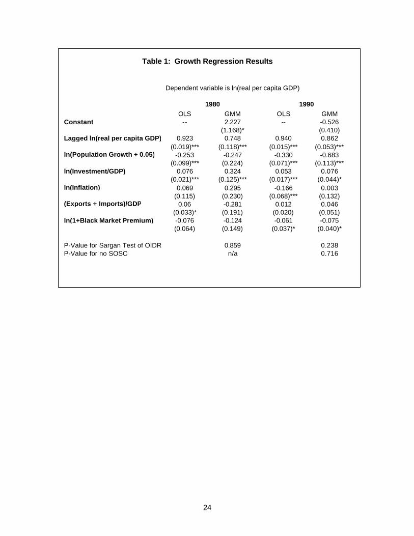
The results of estimating Equation (7) for the two information sets are shown in
Table 1. As a benchmark, we report estimates using OLS on the pooled sample of five-
year averages, and also our preferred specification based on the system GMM estimator
for dynamic panel data. The results are broadly consistent with both intuition and
existing results. The lagged level of income enters significantly with a coefficient less
than one in all cases, and is smaller (implying a higher estimated rate of convergence)
for the GMM estimator. Population growth and investment are always highly significant,
and the magnitude of the estimated coefficients are reasonably stable. Openness and
the black market premium generally enter with the expected signs, but are not
consistently significant. Unfortunately inflation often enters with a perverse positive sign,
although it is only significant when it is negative. The less-than-stellar performance of
the policy variables in the growth regression is somewhat disappointing, and is in part
due to the fact that these are lagged policy variables, rather than contemporaneous.
In summary, the time series model and the growth model can be thought of as
special cases of the same general model in which the log-level of real per capita GDP
7 As a robustness check, we also estimated the growth model using contemporaneous values of theexplanatory variables, and then generated forecasts by inserting the actual future values of the explanatoryvariables into the forecasting equation. This corresponds to the unrealistic assumption that the forecasterhas perfect foresight for all of the explanatory variables when producing growth forecasts. Not surprisingly,(a) the growth model fits somewhat better in sample, and (b) the forecasts generated by this model performsomewhat better, although not by much.

10
follows a first-order autoregressive process around a trend. In the time series model, the
trend is modelled as a simple function of time with at most one shift. In the growth
model, the trend term is interpreted as the steady state of the neoclassical growth
model, and is proxied by variables suggested by the theory. As a result, the forecasts
generated by the growth model are based on more information than the time series
model, since they incorporate proxies for the steady state for each country. Although in
general one would expect that this should lead to superior forecasts, this advantage is to
some extent offset by the fact that the growth model forces the parameters of the model
to be the same across countries, while the time series model allows them to differ across
countries8. Since the balance of these two effects is ambiguous, there is no a priori
reason to prefer one method over the other.
8 Attempting separate within country growth regressions would probably be of limited usefulness because ofinsufficient within-country variation in determinants of long-run growth over our sample period.
11
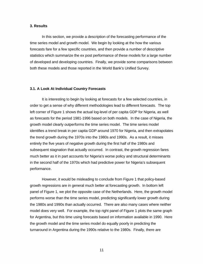
3. Results
In this section, we provide a description of the forecasting performance of the
time series model and growth model. We begin by looking at the how the various
forecasts fare for a few specific countries, and then provide a number of descriptive
statistics which summarize the ex post performance of these models for a large number
of developed and developing countries. Finally, we provide some comparisons between
both these models and those reported in the World Bank’s Unified Survey.
3.1. A Look At Individual Country Forecasts
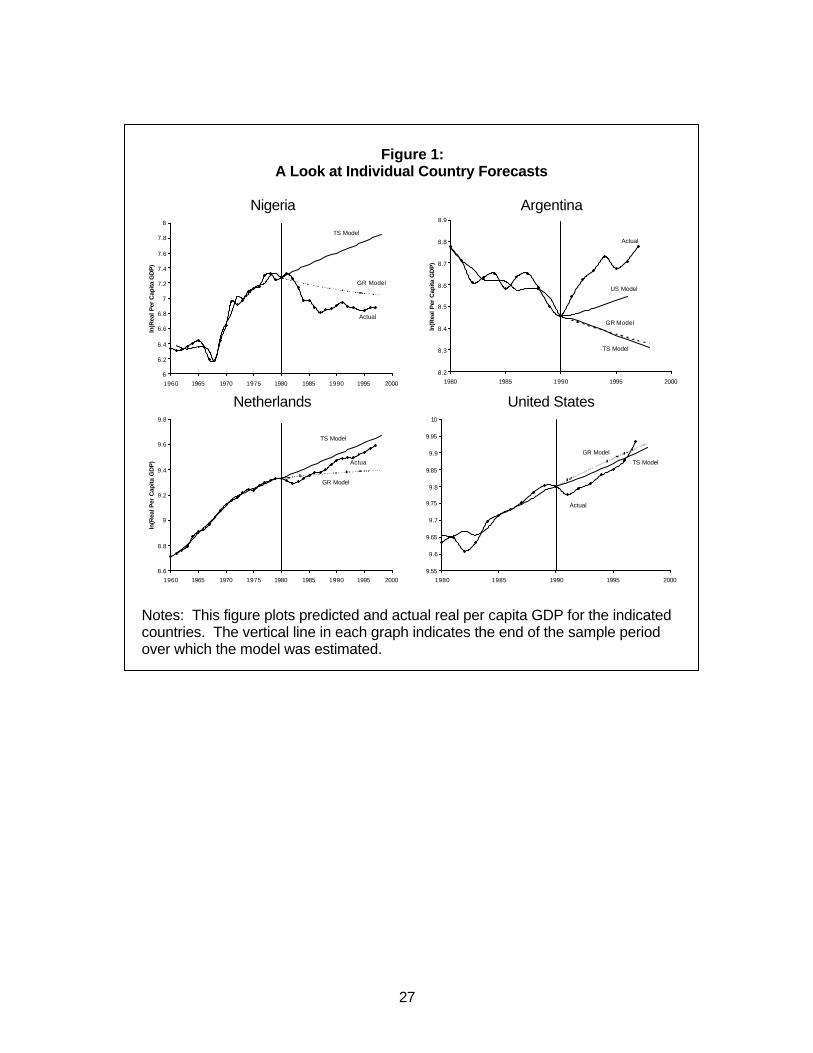
It is interesting to begin by looking at forecasts for a few selected countries, in
order to get a sense of why different methodologies lead to different forecasts. The top
left corner of Figure 1 shows the actual log-level of per capita GDP for Nigeria, as well
as forecasts for the period 1981-1996 based on both models. In the case of Nigeria, the
growth model clearly outperforms the time series model. The time series model
identifies a trend break in per capita GDP around 1970 for Nigeria, and then extrapolates
the trend growth during the 1970s into the 1980s and 1990s. As a result, it misses
entirely the five years of negative growth during the first half of the 1980s and
subsequent stagnation that actually occurred. In contrast, the growth regression fares
much better as it in part accounts for Nigeria’s worse policy and structural determinants
in the second half of the 1970s which had predictive power for Nigeria’s subsequent
performance.
However, it would be misleading to conclude from Figure 1 that policy-based
growth regressions are in general much better at forecasting growth. In bottom left
panel of Figure 1, we plot the opposite case of the Netherlands. Here, the growth model
performs worse than the time series model, predicting significantly lower growth during
the 1980s and 1990s than actually occurred. There are also many cases where neither
model does very well. For example, the top right panel of Figure 1 plots the same graph
for Argentina, but this time using forecasts based on information available in 1990. Here
the growth model and the time series model do equally poorly in predicting the
turnaround in Argentina during the 1990s relative to the 1980s. Finally, there are
12
countries such as the United States where both models perform more or less equally
well (see the bottom right panel of Figure 1).
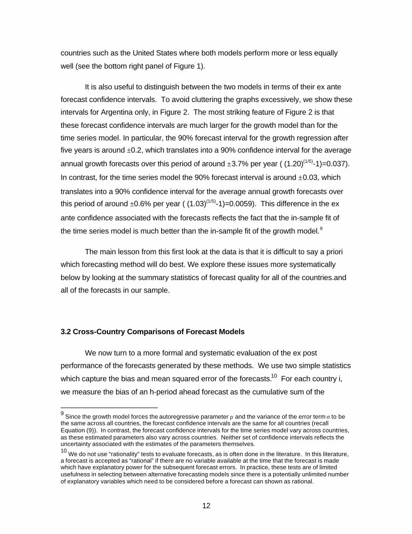
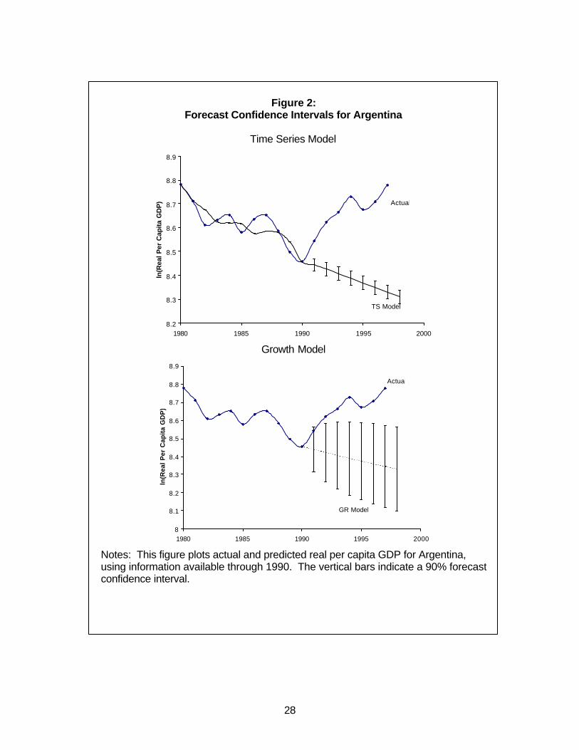
It is also useful to distinguish between the two models in terms of their ex ante
forecast confidence intervals. To avoid cluttering the graphs excessively, we show these
intervals for Argentina only, in Figure 2. The most striking feature of Figure 2 is that
these forecast confidence intervals are much larger for the growth model than for the
time series model. In particular, the 90% forecast interval for the growth regression after
five years is around ±0.2, which translates into a 90% confidence interval for the average
annual growth forecasts over this period of around ±3.7% per year ( (1.20)(1/5)-1)=0.037).
In contrast, for the time series model the 90% forecast interval is around ±0.03, which
translates into a 90% confidence interval for the average annual growth forecasts over
this period of around ±0.6% per year ( (1.03)(1/5)-1)=0.0059). This difference in the ex
ante confidence associated with the forecasts reflects the fact that the in-sample fit of
the time series model is much better than the in-sample fit of the growth model.9
The main lesson from this first look at the data is that it is difficult to say a priori
which forecasting method will do best. We explore these issues more systematically
below by looking at the summary statistics of forecast quality for all of the countries.and
all of the forecasts in our sample.
3.2 Cross-Country Comparisons of Forecast Models
We now turn to a more formal and systematic evaluation of the ex post
performance of the forecasts generated by these methods. We use two simple statistics
which capture the bias and mean squared error of the forecasts.10 For each country i,
we measure the bias of an h-period ahead forecast as the cumulative sum of the
9 Since the growth model forces the autoregressive parameter ρ and the variance of the error term σ to bethe same across all countries, the forecast confidence intervals are the same for all countries (recallEquation (9)). In contrast, the forecast confidence intervals for the time series model vary across countries,as these estimated parameters also vary across countries. Neither set of confidence intervals reflects theuncertainty associated with the estimates of the parameters themselves.10 We do not use “rationality” tests to evaluate forecasts, as is often done in the literature. In this literature,a forecast is accepted as “rational” if there are no variable available at the time that the forecast is madewhich have explanatory power for the subsequent forecast errors. In practice, these tests are of limitedusefulness in selecting between alternative forecasting models since there is a potentially unlimited numberof explanatory variables which need to be considered before a forecast can shown as rational.

13
forecast errors. In order to make this comparable across countries, we scale this sum by
the actual outcomes, resulting in the following cumulative forecast error statistic:
(10)( )
∑
∑
=+
=++ −
= h
1sst,i
h
1sst,it|st,i
t|h,i
y
yyCFE
All other things equal, it is natural to prefer forecasts with cumulative forecast errors near
zero.
Similarly, for each country i we measure the variability or precision of an h-step
ahead forecast using the sum of squared forecast errors. To make this comparable
across countries, we scale it by the sum of squared actual outcomes, resulting in what is
known as the Theil U-statistic:
(11) ( )
∑
∑
=+
=++ −
= h
1s
2st,i
h
1s
2st,it|st,i
t|h,i
y
yyTU
All other things equal, we would prefer forecasting methods with low Theil U-statistics,
since the variability of the forecast errors is low relative to the variability of real per capita
GDP.11
For each country, we calculate the CFE and TU for both forecasting models,
based on information available through 1980, and through 1990, for every possible
forecast horizon. In Figures 3-6 we provide a graphical overview of these many
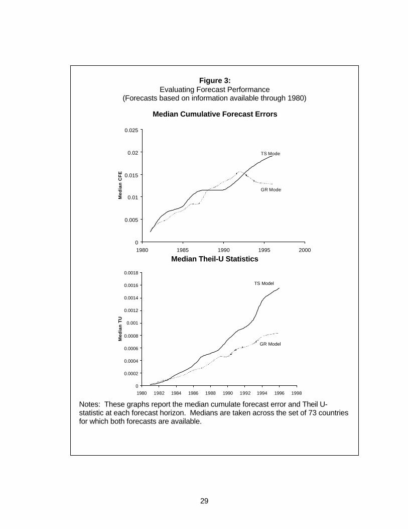
summary statistics of forecast performance. In Figure 3 we consider the sample of 73
countries for which we are able to produce forecasts using all five methods in 1980. 12
We plot time on the horizontal axis, and on the vertical axis, we plot the median across
countries of the two measures of forecast quality discussed above, the CFE (upper
11 As is well known, the MSE of a forecast can be written as the sum of the variance of the forecast errorsplus the bias squared. As such it reflects a particular weighting of bias and precision in assessing forecastquality. However, for many purposes the bias in a forecast is of independent interest. For this reason wereport both the cumulative forecast error and the Theil U statistic for each country.

14
panel), and the TU (lower panel). We report the medians rather than the means, since
for some countries, one model or the other can deliver “crazy” forecasts resulting in very
large TUs or CFEs (in absolute value).
In the upper panel of Figure 3, the time series model and the growth model have
very similar performance in terms of the CFE statistic, which measures the bias in
forecasts. Both models significantly over-predict real per capita GDP -- and do so
increasingly over time13. This occurs because, on average, both models do a rather
poor job of predicting the worldwide slowdown in growth during the first half of the
1980s. To interpret the magnitude of this bias, recall that the vertical axis measures
logarithm of real per capita GDP. Since, for example, the cumulative median bias in the
level of forecasted real per capita GDP after five years is around 7% of per capita GDP,
this translates into an upward bias in average annual growth forecasts over this period of
around 1.4% per year ( (1.07)(1/5)-1)=0.0136).
Turning to the TU statistics in the lower panel, there is a somewhat clearer
distinction between the two models. At all forecast horizons, the growth model delivers a
lower variablity of forecast errors, as reflected in lower TU statistics. This gap between
the two models widens over time, suggesting that the relative performance of the growth
model is better for longer-term growth forecasts. In contrast, at short horizons, e.g. less
than 5 years, the performance of the two models is rather similar. Somewhat
surprisingly, the relative performance of these models according to both criteria is similar
in a smaller sample of 59 developing countries for which we have forecasts from both
models. The graphs summarizing these results are omitted for brevity.
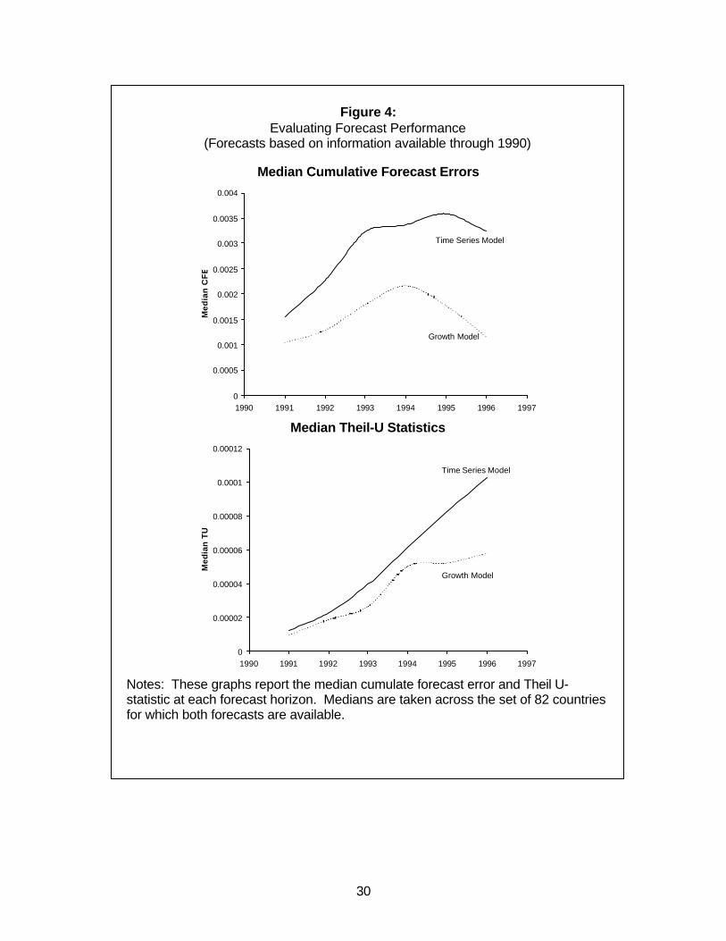
In Figure 4 we do the same exercise, but for forecasts based on information
available through 1990, using a slightly larger sample of 82 countries. As in the 1980s,
the forecasts of both models are on average biased upwards, although less so than in
the 1980s forecasts (note that the units of the vertical axis are very different in Figures 4
and 3). The median bias in the forecasts is never greater than 0.4% of GDP. In
12 Although we can produce the time series forecasts for all 112 countries in our data set, we have completedata on all of the explanatory variables required for the growth regression in 1980 for only 73 countries, andfor 82 countries in 1990.
15
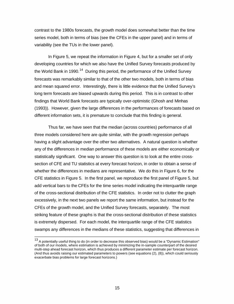
contrast to the 1980s forecasts, the growth model does somewhat better than the time
series model, both in terms of bias (see the CFEs in the upper panel) and in terms of
variability (see the TUs in the lower panel).
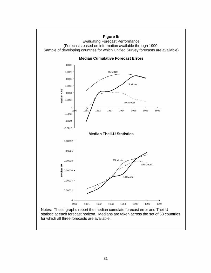
In Figure 5, we repeat the information in Figure 4, but for a smaller set of only
developing countries for which we also have the Unified Survey forecasts produced by
the World Bank in 1990.14 During this period, the performance of the Unified Survey
forecasts was remarkably similar to that of the other two models, both in terms of bias
and mean squared error. Interestingly, there is little evidence that the Unified Survey’s
long term forecasts are biased upwards during this period. This is in contrast to other
findings that World Bank forecasts are typically over-optimistic (Ghosh and Minhas
(1993)). However, given the large differences in the performances of forecasts based on
different information sets, it is premature to conclude that this finding is general.
Thus far, we have seen that the median (across countries) performance of all
three models considered here are quite similar, with the growth regression perhaps
having a slight advantage over the other two alternatives. A natural question is whether
any of the differences in median performance of these models are either economically or
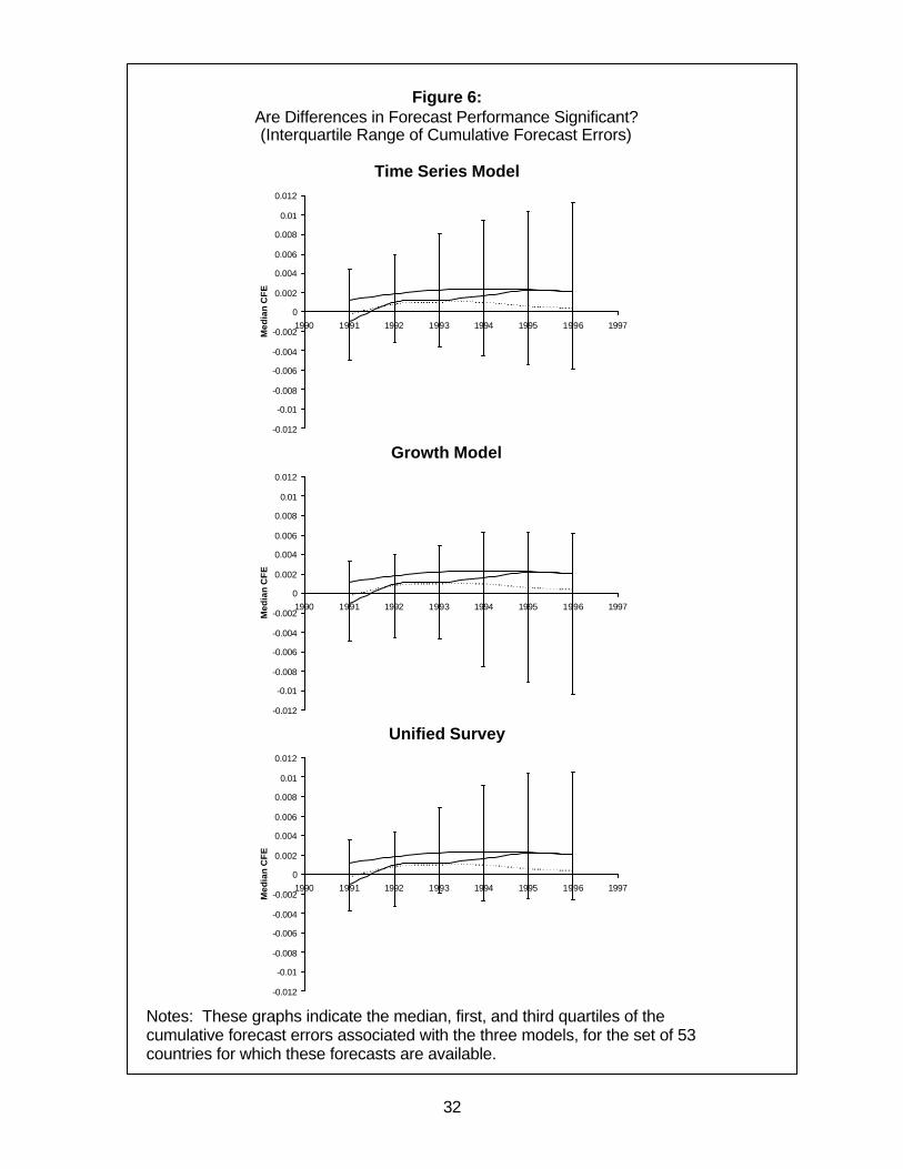
statistically significant. One way to answer this question is to look at the entire cross-
section of CFE and TU statistics at every forecast horizon, in order to obtain a sense of
whether the differences in medians are representative. We do this in Figure 6, for the
CFE statistics in Figure 5. In the first panel, we reproduce the first panel of Figure 5, but
add vertical bars to the CFEs for the time series model indicating the interquartile range
of the cross-sectional distribution of the CFE statistics. In order not to clutter the graph
excessively, in the next two panels we report the same information, but instead for the
CFEs of the growth model, and the Unified Survey forecasts, separately. The most
striking feature of these graphs is that the cross-sectional distribution of these statistics
is extremely dispersed. For each model, the interquartile range of the CFE statistics
swamps any differences in the medians of these statistics, suggesting that differences in
13 A potentially useful thing to do (in order to decrease this observed bias) would be a “Dynamic Estimation”of both of our models, where estimation is achieved by minimizing the in-sample counterpart of the desiredmulti-step ahead forecast horizon, which thus produces a different parameter estimate per forecast horizon.(And thus avoids raising our estimated parameters to powers (see equations (2), (8)), which could seriouslyexacerbate bias problems for large forecast horizons.)
16
median performance are highly unlikely to be of statistical or practical relevance. Similar
graphs indicating the cross-country dispersion in the TU statistics (not shown for brevity)
lead to a similar conclusion that the cross-country variation in model performance is
large relative to the differences in median performance.
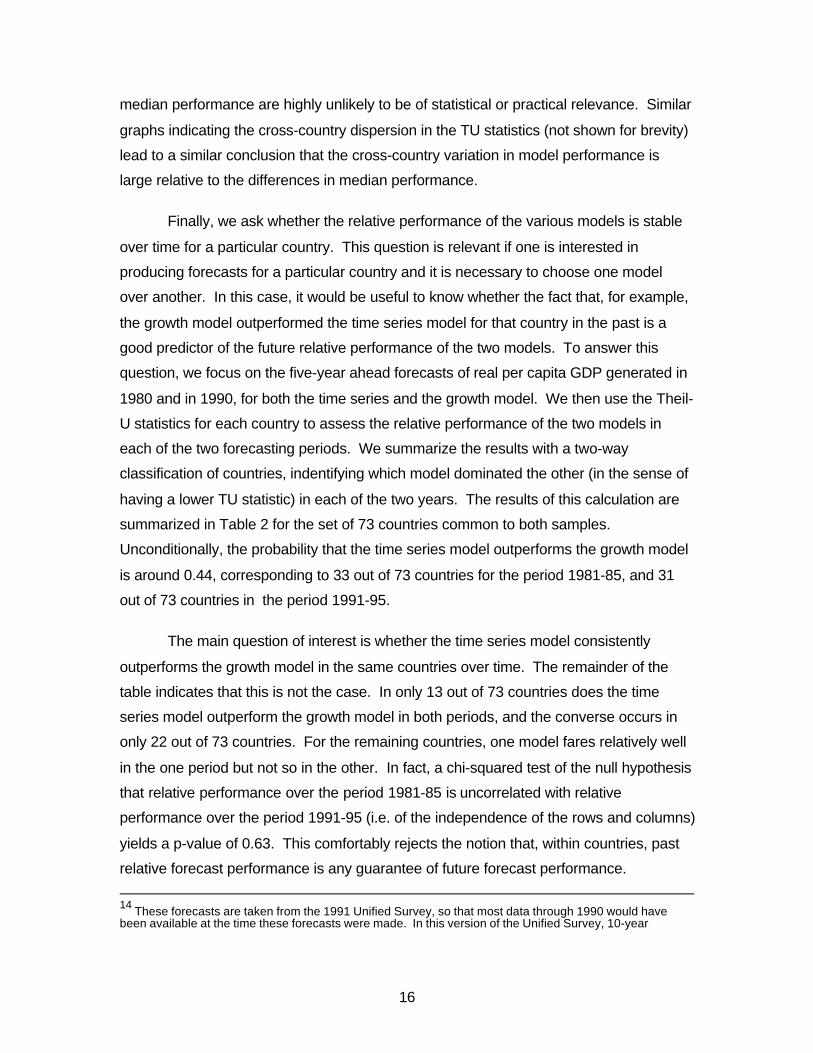
Finally, we ask whether the relative performance of the various models is stable
over time for a particular country. This question is relevant if one is interested in
producing forecasts for a particular country and it is necessary to choose one model
over another. In this case, it would be useful to know whether the fact that, for example,
the growth model outperformed the time series model for that country in the past is a
good predictor of the future relative performance of the two models. To answer this
question, we focus on the five-year ahead forecasts of real per capita GDP generated in
1980 and in 1990, for both the time series and the growth model. We then use the Theil-
U statistics for each country to assess the relative performance of the two models in
each of the two forecasting periods. We summarize the results with a two-way
classification of countries, indentifying which model dominated the other (in the sense of
having a lower TU statistic) in each of the two years. The results of this calculation are
summarized in Table 2 for the set of 73 countries common to both samples.
Unconditionally, the probability that the time series model outperforms the growth model
is around 0.44, corresponding to 33 out of 73 countries for the period 1981-85, and 31
out of 73 countries in the period 1991-95.
The main question of interest is whether the time series model consistently
outperforms the growth model in the same countries over time. The remainder of the
table indicates that this is not the case. In only 13 out of 73 countries does the time
series model outperform the growth model in both periods, and the converse occurs in
only 22 out of 73 countries. For the remaining countries, one model fares relatively well
in the one period but not so in the other. In fact, a chi-squared test of the null hypothesis
that relative performance over the period 1981-85 is uncorrelated with relative
performance over the period 1991-95 (i.e. of the independence of the rows and columns)
yields a p-value of 0.63. This comfortably rejects the notion that, within countries, past
relative forecast performance is any guarantee of future forecast performance.
14 These forecasts are taken from the 1991 Unified Survey, so that most data through 1990 would havebeen available at the time these forecasts were made. In this version of the Unified Survey, 10-year
17
4. Implications
In this section we take up two questions suggested by the results of the previous
section. First, given that both the time series and the growth models perform
comparably, is it possible to combine them in some way to arrive at better forecasts?
Second, does either model perform well in absolute (as opposed to relative) terms?
4.1 Can Alternative Forecasting Models “Learn” From Each Other?
Thus far, we have seen that there is little clear evidence suggesting that we
should select one model over another as a forecasting tool. Rather than restrict
ourselves to selecting one model over another, a more constructive approach is to ask
whether some combination of models leads to better forecasts. We do this using tests of
forecast combination and encompassing. Intuitively, these tests ask whether alternative
forecasting models can “learn” from each other. If they do, this suggests that superior
forecasts can be obtained by combining the two models in some way.
Formally, suppose that both the time series and the growth model generate
forecasts that are informative for future real per capita GDP, so that we can write future
real per capita GDP as a linear combination of the two forecasts plus an error term:
(12) st,iTS
t|st,iGR
t|st,ist,i uy)1(yy ++++ +⋅β−+⋅β+α=
where the superscripts TS and GR differentiate between the forecasts of the time series
and growth models. 15 We can then test the null hypothesis that the time series model
forecast-encompasses the growth model by testing the null that β=0. The intuition for
this test is straightforward, since it simply asks whether the variation in the growth-
regression based forecasts that is orthogonal to the time series forecasts has any useful
explanatory power for actual outcomes. If it does not, then the time series model
“encompasses” the growth model in the sense that the growth model’s forecasts provide
average annual growth projections were produced, and we use these average annual growth rates toforecast growth for every year through 1996.
18
no additional predictive power for actual output. Conversely, we can test whether the
growth model encompasses the time series model by testing whether β=1.
We implement these tests for the time series and growth models discussed
above as follows. For every forecast horizon, we estimate Equation (12) cross-
sectionally, and test the two null hypotheses that each model encompasses the other. 16
The results of the cross-sectional regressions are shown in Table 3. In general, we reject
the null hypothesis that either model encompasses the other at short forecast horizons,
suggesting that both models can benefit from incorporating features of the other.
Interestingly, as the forecast horizon increases, we do not reject the null hypothesis that
the growth model encompasses the time series model (i.e. β=1) , but not the converse.
This is consistent with the notion that long-run growth regressions do a better job of
predicting long-term growth.
These results strongly suggest that there are benefits to combining the
information from both forecasting models. However, it is less clear exactly how this
should be done. A simple approach would be to use some weighted average of
forecasts from the two models. There is some empirical evidence in other contexts that
weighted (or even unweighted) averages can outperform the components of the average
(e.g. Stock & Watson (1998)). However, Diebold (1989) stresses that there is no
guarantee that this will be the case in general. Since neither model individually does a
very good job at capturing the “true” underlying data generating process, there is no
reason to believe that a combination of the two will do so on a consistent basis. For
example, the large negative intercepts in the encompassing regressions for the 1980s
forecasts reflect the large ex post positive bias in these forecasts. However, if we were
to use this information to systematically lower all growth forecasts for the 1990s (as the
encompassing regression might suggest), we would have ended up significantly
underpredicting growth in the 1990s.
15 The restriction that the coefficients on the two models sum to one is not essential. Estimating theseencompassing regressions without such a restriction leads to very similar results.16 We also carry out these tests using the time series of forecast errors for each country, from the forecastsbased on information available through 1980. For each country, we estimated rolling regressions, startingwith the time series of the first 10 forecast errors over the period 1981-90, and continuing through the entiretime series of errors through 1997. The results of this exercise were consistent with the cross-sectionalresults. At short horizons, neither model encompassed the other. However, it was more likely that thegrowth model encompassed the time series model at long horizons than the other way around.

19
Instead, a more compelling approach is to combine the information sets on which
the forecasts are based, rather than combine the forecasts themselves (Clements and
Hendry (1998), Diebold (1989)). For example, a natural way to combine the two models
would be to consider a hybrid time series model which (a) includes additional
explanatory variables that our time series model omits, and (b) relaxes the restriction of
the growth models that the parameter estimates are equal across countries. An
example of such a modelling strategy might be a non-structural vector autoregression in
several key macroeconomic variables, estimated country-by-country. Forecasts based
on such a combined information set are more likely to encompasses alternatives since
they making optimal use of all of the (useful) available information in both information
sets.
4.2 Formal Tests of Predictive Failure
Thus far, our emphasis has been on comparing the relative performance of
alternative forecasting models. We now turn to a rather different question: is the
absolute performance of these forecasting models adequate? Alternatively, is the ex
post performance of these forecasting models good enough (or bad enough) that we
should continue to use some combination of these models (or search for other
forecasting models)?
In principle, this question can be answered using the test of predictive failure
developed by Box and Tiao (1976). Intuitively, this test asks whether the deviations
between forecasts and actuality are large relative to the forecast confidence intervals
generated ex ante. To see how this works, consider the case of Argentina, where we
have already seen the forecast confidence intervals in Figure 2. For the case of a one-
step ahead forecast, the Box-Tiao test simply asks whether the actual outcome of real
per capita GDP falls within the ex ante confidence interval generated by the forecaster.
If it does, we do not reject the null hypothesis that the forecasting model is correctly
specified, since, roughly speaking, the actual outcome fell within the range that was
expected a priori. This, however, should not be taken as an endorsement of the model
either, since failure to reject the null hypothesis may simply reflect large ex ante
20
confidence intervals generated by a model that fits very poorly within-sample. If in
contrast the actual outcome falls outside the range predicted by the forecaster, the Box-
Tiao test rejects the model.
In the case of Argentina, we see that for the one-year ahead forecast, i.e. the
forecast of real per capita GDP in 1991 based on information in 1990, falls inside the
confidence interval of the growth model, but outside the confidence interval of the time
series model. The Box-Tiao test therefore suggests that we should reject the time series
model, but not the growth model, as a forecasting tool. We have implemented the
version of the Box-Tiao test appropriate for multi-step forecasts for all countries, and we
find a similar pattern to that observed in Argentina.17 For the great majority of countries,
the Box-Tiao test suggests that we should reject the time series model. For the growth
model, the Box-Tiao test rejects the growth model for about half of the countries, and
fails to reject for the other half. 18
Is this conclusion warranted? As noted above, the Box - Tiao test may fail to
reject a model simply because the model is very imprecise ex ante. Indeed, in our
context, and as is clear from Figure 2, the main reason why the growth model is not
rejected by the Box-Tiao test is because the ex-ante forecast confidence intervals
associated with this model are so large as to render the accompanying growth forecasts
virtually meaningless. We have already noted that the growth regression typically
generates ex ante forecast intervals of plus or minus four percent per year around a
typical 5-year ahead growth forecast. This spans almost the entire range of actual
growth performance in most periods. Conversely, the time series model fares relatively
poorly according to the Box-Tiao criterion for assessing the significance of predictive
failure because the ex ante confidence intervals associated with the time series model
are far smaller than those of the growth model. This reflects the fact that the time series
model tends to “over-fit” the data in sample. Given that the parameters of the time
series model are typically rather imprecisely estimated (especially the date of the trend
break), forecast confidence intervals which take this into account would give a more
17 In particular, Box and Tiao (1976) show that for a process with Gaussian innovations,
t1
t e'e −Ω has a
χ2(h) distribution, where e t is the hx1 vector of forecast errors through h and Ω=E[e t et’]. Given theexpressions for the forecast errors in Equations (3) and (9) and the corresponding estimates of ρi, it ispossible to obtain an estimate of Ω and compute the appropriate test statistic.

21
reasonable picture of the ex ante uncertainty of this model’s forecasts. As a result, the
Box-Tiao test would be less likely to reject this model as a forecasting tool.
18 Recall that the forecast confidence intervals are the same across countries for the growth model. For thetime series model, there is some variation, but since in general the time series model fits the data very wellin-sample, the forecast confidence intervals tend to be quite small for all countries.
22
5. Conclusions
In this paper, we have considered the relative performance of two simple
forecasting models for real per capita GDP in a large sample of developed and
developing countries: a univariate time series model for real per capita GDP, and a
cross-country growth regression model. The most striking finding of this paper is that
neither model clearly dominates as a forecasting tool. Median (across countries)
differences in the forecasting performance of the two models are typically very small
relative to the cross-country variation in relative model performance. Moreover, both
absolute and relative model performance is very unstable over time. Both models
significantly overpredict growth in the 1980s, but do not in the 1990s. Within countries,
past relative forecast performance is uncorrelated with future relative forecast
performance.
These results indicate that it is very difficult to choose the “best” forecasting
model for a particular country or group of countries. Instead of attempting such a choice,
our results suggest that there are potential benefits from combining the two forecasting
methodologies. Forecast encompassing tests indicate that the forecasts of both models
are jointly informative for actual outcomes, especially at shorter horizons. A natural way
to proceed would be to combine the information sets from the two models in some way.
In particular, vector autoregressions in a small set of key macroeconomic variables,
estimated country-by-country, may improve over the forecast performance of both
models. The advantage of such an approach over the univariate time series models is
that it draws on a larger information set. This approach can potentially also improve
over forecasts based on cross-country growth regressions by relaxing the restrictive
assumption that the parameters of the model are equal across countries.
23
References
Arellano, Manuel and Olympia Bover (1995). “Another Look at the Instrumental VariableEstimation of Error-Components Models”. Journal of Econometrics. 68:29-51.
Artis, Michael (1996). “How Accurate are the IMF’s Short Term Forecasts? AnotherExamination of the World Economic Outlook”. Manuscript: European UniversityInstitute.
Box, G.E.P., and G.C Tiao (1976), “Comparison of Forecast and Actuality”, AppliedStatistics, 25, 195-200.
Clements, M, and David Hendry (1998), “Forecasting Economic Time Series”, CUP.
Diebold, F (1989), “Forecast combination and encompassing: Reconciling two divergentliteratures”, International Journal of Forecasting, 5, 589-592.
Diebold, F, and L. Kilian (1999), “Unit root tests are useful for selecting forecastingmodels”, NBER WP 6928.
Ghosh, Atish and Tanya S. Minhas (1993). “How Good Are World Bank Projections? APost-Mortem for the Period 1975-1991.
Stock, J.H., and M. Watson (1998), “A Comparison of Linear and Nonlinear UnivariateModels for Forecasting Macroeconomic Time Series”, NBER Working Paper6607.
Verbeek, Jos (1999). “The World Bank’s Unified Survey Projections: How Accurate AreThey? An Ex-Post Evaluation of US91-US97”. World Bank Policy ResearchDepartment Working Paper No. 2071.
Vogelsang, T.J. (1997), “Wald-Type Tests for Detecting Breaks in the Trend Function ofa Dynamic Time Series”, Econometric Theory, 13, 818-849.
24
Table 1: Growth Regression Results
Dependent variable is ln(real per capita GDP)
OLS GMM OLS GMMConstant -- 2.227 -- -0.526
(1.168)* (0.410)Lagged ln(real per capita GDP) 0.923 0.748 0.940 0.862
(0.019)*** (0.118)*** (0.015)*** (0.053)***ln(Population Growth + 0.05) -0.253 -0.247 -0.330 -0.683
(0.099)*** (0.224) (0.071)*** (0.113)***ln(Investment/GDP) 0.076 0.324 0.053 0.076
(0.021)*** (0.125)*** (0.017)*** (0.044)*ln(Inflation) 0.069 0.295 -0.166 0.003
(0.115) (0.230) (0.068)*** (0.132)(Exports + Imports)/GDP 0.06 -0.281 0.012 0.046
(0.033)* (0.191) (0.020) (0.051)ln(1+Black Market Premium) -0.076 -0.124 -0.061 -0.075
(0.064) (0.149) (0.037)* (0.040)*
P-Value for Sargan Test of OIDR 0.859 0.238P-Value for no SOSC n/a 0.716
1980 1990

25
Table 2: Persistence of Relative Forecast Performance
1991-95TS Dominates GR Dominates Total
1981 TS Dominates 13 20 33-1985 GR Dominates 18 22 40
Total 31 42 73
P-Value for Chi-Squared Test of Independence: 0.63
Notes: This table reports the relative forecast performance of the time series model(TS) and the growth model (GR), for 5-year growth forecasts for 1981-85 and 1991-95.The cells of the table indicate the number of countries for which the TU statistic of theTB model is lower than that of the GR model (TS Dominates), and conversely thenumber of countries for which the TU statistic of the GR model is lower (GR Dominates)during the indicated forecast periods.

26
Table 3: Forecast Encompassing Tests
P-Value for:α se(α) β se(β) Ho: β=0 Ho: β=1
Forecast Origin = 1980
1981 -0.015 0.006 0.501 0.179 0.005 0.0051982 -0.057 0.01 0.527 0.163 0.001 0.0041983 -0.095 0.016 0.654 0.165 0.000 0.0361984 -0.112 0.02 0.763 0.154 0.000 0.1241985 -0.121 0.022 0.71 0.138 0.000 0.0361986 -0.124 0.026 0.783 0.132 0.000 0.1001987 -0.132 0.029 0.83 0.127 0.000 0.1811988 -0.133 0.032 0.799 0.122 0.000 0.0991989 -0.136 0.036 0.804 0.121 0.000 0.1051990 -0.14 0.039 0.821 0.117 0.000 0.1261991 -0.15 0.04 0.838 0.109 0.000 0.1371992 -0.164 0.044 0.854 0.108 0.000 0.1761993 -0.177 0.047 0.88 0.106 0.000 0.2581994 -0.177 0.05 0.897 0.105 0.000 0.3271995 -0.166 0.052 0.917 0.101 0.000 0.4111996 -0.149 0.055 0.934 0.099 0.000 0.5051997 -0.164 0.057 0.89 0.099 0.000 0.267
Forecast Origin = 1990
1991 -0.004 0.005 0.603 0.274 0.028 0.1471992 -0.013 0.009 0.563 0.237 0.018 0.0651993 -0.016 0.012 0.797 0.221 0.000 0.3581994 -0.007 0.013 0.766 0.181 0.000 0.1961995 0.004 0.014 0.807 0.157 0.000 0.2191996 0.021 0.017 0.842 0.152 0.000 0.2991997 0.028 0.017 0.885 0.135 0.000 0.394
Notes: This table reports the results from estimating the following regression:
st,iTS
t|st,iGR
t|st,ist,i uy)1(yy ++++ +⋅β−+⋅β+α=
cross-sectionally for each of the indicated years. The last two columns report the p-values corresponding to the null hypothesis that the time series model encompassesthe growth model (β=0) and that the growth model encompasses the time series model(β=1).
27
Figure 1:A Look at Individual Country Forecasts
Nigeria Argentina
6
6.2
6.4
6.6
6.8
7
7.2
7.4
7.6
7.8
8
1960 1965 1970 1975 1980 1985 1990 1995 2000
ln(R
eal P
er C
apita
GD
P)
Actual
GR Model
TS Model
8.2
8.3
8.4
8.5
8.6
8.7
8.8
8.9
1980 1985 1990 1995 2000
ln(R
eal P
er C
apita
GD
P)
GR Model
Actual
US Model
TS Model
Netherlands United States
8.6
8.8
9
9.2
9.4
9.6
9.8
1960 1965 1970 1975 1980 1985 1990 1995 2000
ln(R
eal P
er C
apita
GD
P)
TS Model
GR Model
Actual
9.55
9.6
9.65
9.7
9.75
9.8
9.85
9.9
9.95
10
1980 1985 1990 1995 2000
TS Model
GR Model
Actual
Notes: This figure plots predicted and actual real per capita GDP for the indicatedcountries. The vertical line in each graph indicates the end of the sample periodover which the model was estimated.
28
Figure 2:Forecast Confidence Intervals for Argentina
Time Series Model
8.2
8.3
8.4
8.5
8.6
8.7
8.8
8.9
1980 1985 1990 1995 2000
ln(R
eal P
er C
apita
GD
P) Actual
TS Model
Growth Model
8
8.1
8.2
8.3
8.4
8.5
8.6
8.7
8.8
8.9
1980 1985 1990 1995 2000
ln(R
eal
Per
Cap
ita
GD
P)
Actual
GR Model
Notes: This figure plots actual and predicted real per capita GDP for Argentina,using information available through 1990. The vertical bars indicate a 90% forecastconfidence interval.
29
Figure 3:Evaluating Forecast Performance
(Forecasts based on information available through 1980)
Median Cumulative Forecast Errors
0
0.005
0.01
0.015
0.02
0.025
1980 1985 1990 1995 2000
Med
ian
CF
E
TS Model
GR Model
Median Theil-U Statistics
0
0.0002
0.0004
0.0006
0.0008
0.001
0.0012
0.0014
0.0016
0.0018
1980 1982 1984 1986 1988 1990 1992 1994 1996 1998
Med
ian
TU
TS Model
GR Model
Notes: These graphs report the median cumulate forecast error and Theil U-statistic at each forecast horizon. Medians are taken across the set of 73 countriesfor which both forecasts are available.
30
Figure 4:Evaluating Forecast Performance
(Forecasts based on information available through 1990)
Median Cumulative Forecast Errors
0
0.0005
0.001
0.0015
0.002
0.0025
0.003
0.0035
0.004
1990 1991 1992 1993 1994 1995 1996 1997
Med
ian
CF
E
Time Series Model
Growth Model
Median Theil-U Statistics
0
0.00002
0.00004
0.00006
0.00008
0.0001
0.00012
1990 1991 1992 1993 1994 1995 1996 1997
Med
ian
TU
Time Series Model
Growth Model
Notes: These graphs report the median cumulate forecast error and Theil U-statistic at each forecast horizon. Medians are taken across the set of 82 countriesfor which both forecasts are available.
31
Figure 5:Evaluating Forecast Performance
(Forecasts based on information available through 1990,Sample of developing countries for which Unified Survey forecasts are available)
Median Cumulative Forecast Errors
-0.0015
-0.001
-0.0005
0
0.0005
0.001
0.0015
0.002
0.0025
0.003
1990 1991 1992 1993 1994 1995 1996 1997
Med
ian
CF
E
TS Model
US Model
GR Model
Median Theil-U Statistics
0
0.00002
0.00004
0.00006
0.00008
0.0001
0.00012
1990 1991 1992 1993 1994 1995 1996 1997
Med
ian
TU
TS Model
US Model
GR Model
Notes: These graphs report the median cumulate forecast error and Theil U-statistic at each forecast horizon. Medians are taken across the set of 53 countriesfor which all three forecasts are available.
32
Figure 6:Are Differences in Forecast Performance Significant?(Interquartile Range of Cumulative Forecast Errors)
Time Series Model
-0.012
-0.01
-0.008
-0.006
-0.004
-0.002
0
0.002
0.004
0.006
0.008
0.01
0.012
1990 1991 1992 1993 1994 1995 1996 1997
Med
ian
CF
E
Growth Model
-0.012
-0.01
-0.008
-0.006
-0.004
-0.002
0
0.002
0.004
0.006
0.008
0.01
0.012
1990 1991 1992 1993 1994 1995 1996 1997
Med
ian
CF
E
Unified Survey
-0.012
-0.01
-0.008
-0.006
-0.004
-0.002
0
0.002
0.004
0.006
0.008
0.01
0.012
1990 1991 1992 1993 1994 1995 1996 1997
Med
ian
CF
E
Notes: These graphs indicate the median, first, and third quartiles of thecumulative forecast errors associated with the three models, for the set of 53countries for which these forecasts are available.