growth impact of government consumption, … · university of cape coast . growth impact of...

UNIVERSITY OF CAPE COAST

GROWTH IMPACT OF GOVERNMENT CONSUMPTION, TRANSFER

AND INTEREST PAYMENTS IN GHANA

BY

EDMUND ADINKRA DARKO

Thesis submitted to the Department of Economics of the College of

Humanities and Legal Studies, University of Cape Coast, in partial fulfilment

of the requirements for award of Master of Philosophy Degree in Economics.

DECEMBER 2016

Digitized by UCC, Library

ii

DECLARATION

Candidate’s Declaration

I hereby declare that this thesis is the result of my own original work and that

no part of it has been presented for another degree in this university or

elsewhere.

Candidate’s Name: Edmund Adinkra Darko

Signature: ………………………............. Date: ………………………………

Supervisors’ Declaration

We hereby declare that the preparation and presentation of the thesis were

supervised in accordance with the guidelines on supervision of thesis laid

down by the University of Cape Coast.

Principal Supervisor’s Name: Dr. William G. Brafu-Insaidoo

Signature: …………………………........... Date: ………….……………….

Co-Supervisor’s Name: Dr. Ferdinand M. Ahiakpor

Signature: ....………………………......... Date: ……………………….........


iii

ABSTRACT

The study examined the growth impact of government consumption,

interest and transfer payments in Ghana. A quarterly time series data from

1984 to 2015 was utilised. The maximum likelihood estimation (MLE)

technique was employed, and cointegration among the variables was

established within the framework of autoregressive distributed lag (ARDL). A

Pair-wise Granger-causality test was adopted to explore the direction of

causality between government expenditure components (consumption, transfer

and interest payments) and economic growth.

The ARDL results revealed that government interest payments and

consumption expenditure negatively impact economic growth in both long run

and short run. However, government transfers indicated a positive significant

relationship with growth of output. The results of the Granger causality test

established a bi-directional causality between government interest payment

and economic growth. Unidirectional causalities running from government

consumption expenditure and transfer payment to economic growth were also

established.

Considering the findings, the following recommendations are offered:

Government must ensure that loans taken are properly utilised so that returns

from such use will be used to cater for the loans and the associated interest.

Government should cut down its consumption. Lastly, government through the

Department of Social Welfare should increase and regularize its general

transfer payment in order to elevate the vulnerable groups from extreme

poverty.


iv

KEY WORDS

Growth impact

Government consumption expenditure

Government transfer payment

Government interest payment


v

ACKNOWLEDGEMENTS

My heartfelt appreciation goes to my supervisors: Dr. William G.

Brafu-Insaidoo and Dr. Ferdinand M. Ahiakpor for their readings, constructive

comments and candid suggestions which made this thesis a success.

I owe a great debt of gratitude to Mr. Martin Asiedu, Mr. Joseph Adjei-

Manu, and Mr Daniel Abina Dwaase for the support during this study period.

I am most grateful to Dr. Isaac Bentum-Ennin, Mr. Nkansah K. Darfor,

Mr. Michael Asiamah and Mr. Peter Partey Anti for their concern and deepest

assistance during the process.

I am again grateful to the African Economic Research Consortium

(AERC) for the sponsorship in the Joint Facility for Electives (JFE) in Arusha

Tanzania.

Lastly, I acknowledge all my course mates for the assistance in diverse

ways. Nonetheless, I am personally responsible for any shortcomings of this

thesis.


vi

DEDICATION

To my mother and my siblings for their support and encouragement.


vii

TABLE OF CONTENTS

Content Page

DECLARATION i

ABSTRACT iii

KEY WORDS iv

ACKNOWLEDGEMENTS v

DEDICATION vi

TABLE OF CONTENTS vii

LIST OF TABLES xi

LIST OF FIGURES xii

LIST OF ACRONYMS xiii

CHAPTER ONE: INTRODUCTION 1

Background to the Study 1

Statement of the Problem 7

Purpose of the study 11

Research Hypotheses 11

Significance of the study 12

Scope of the study 13

Organization of the study 13

CHAPTER TWO: REVIEW OF RELATED LITERATURE 14

Introduction 14

Theoretical Literature Review 14


viii

Theoretical Background of Government Expenditure and Economic Growth

Nexus 14

Government Expenditure and Economic Growth: Aggregate Demand and

Aggregate Supply Framework 17

Review of some Growth Models 19

Neoclassical Growth Theories 19

Peacock-Shaw (1971) Model 20

Solow-Swan (1956) Model 23

Endogenous Growth Models 25

Afonso-Alegre (2008) Growth Model 29

The Role of Government in Economic Growth 32

The Minimal Government Argument 32

The Market versus the Government 34

Some Theories of Government Expenditure Growth 36

Musgrave and Rostow's Development Model 36

The Wagner’s Law 37

The Classical versus the Keynesian Argument 38

Peacock and Wiseman Hypothesis 40

Government Expenditure and Economic Growth in Ghana 41

Empirical Literature Review 47

Summary of the Literature Review 65

CHAPTER THREE: METHODOLOGY 67

Introduction 67

Research Design 67

Theoretical Model Specification 68

Empirical Model Specification 69

Definition and Measurement of Variables 71


ix

Nature and Sources of Data 75

Estimation Technique 76

Unit Root Tests 77

Cointegration Test 79

Post Estimation/Diagnostics Test 85

Granger Causality Test 86

Summary of the Methodology 87

CHAPTER FOUR: RESULTS AND DISCUSSION 89

Introduction 89

Descriptive Statistics 89

Unit Root Test 90

Bounds Test for Cointegration 94

Long Run Relationship 95

Short Run Relationship 101

Model Diagnostics and Stability Tests 107

Granger Causality Tests 109

Conclusion 111

CHAPTER FIVE: SUMMARY, CONCLUSIONS AND

RECOMMENDATIONS 114

Introduction 114

Summary 114

Conclusions 117

Recommendations 118

Limitations of the Study 119

Direction for Future Research 120


x

REFERENCES 122

APPENDICES 138

APPENDIX A 138

GRAPH OF VARIABLES AT LEVEL 138

APPENDIX B 139

GRAPH OF VARIABLES AT FIRST DIFFERENCE 139


xi

LIST OF TABLES

Table Page

1: Summary Statistics of the Variables 90

2: Results of Unit Root Test with constant and trend: ADF Test 92

3: Results of Unit Root Test with intercept and trend: PP Test 93

4: Results of Bounds Tests for the Existence of Cointegration 94

5: Estimated Long-Run Coefficients using the ARDL Approach 96

6: Estimated Short-Run Coefficients 102

7: Model Diagnostics 107

8: Results of Pair-wise Granger Causality Tests 110


xii

LIST OF FIGURES

Figure Page

1: Trend of Real GDP 4

2: Trend of Government Interest Payment 5

3: Trend of Government Transfer Payment 6

4: Trend of Government Consumption Expenditure (% of GDP) 6

5: Plot of Cumulative Sum of Recursive Residuals 108

6: Plot of Cumulative Sum of Squares of Recursive Residuals 109


xiii

LIST OF ACRONYMS

AD Aggregate Demand

ADF Augmented Dickey-Fuller

AIC Akaike Information Criterion

ARDL Autoregressive Distributed Lag

ARMA Autoregressive Moving Average

AS Aggregate Supply

CPI Consumer Price Index

CUSUM Cumulative Sum of Recursive Residuals

CUSUMSQ Cumulative Sum of Squares of Recursive Residual

CXP Government Consumption Expenditure

DW Durbin Watson

ECM Error Correction Model

ECT Error Correction Term

ERP Economic Recovery Programme

EU European Union

FMOLS Fully Modified Ordinary Least Squares

GCC Gulf Cooperation Council

GDP Gross Domestic Product

GMM Generalized Method of Moments

GSS Ghana Statistical Service

GXP Aggregate Government Expenditure

HIPC Highly Indebted Poor Country

IMF International Monetary Fund

IP Interest Payment


xiv

LEAP Livelihood Empowerment Against Poverty

LM Lagrange Multiplier

MLE Maximum Likelihood Estimation

MoFEP Ministry of Finance and Economic Planning

NX Net Expotrs

OECD Organisation for Economic and Cooperative Development

OLS Ordinary Least Square

P P Phillip-Perron

RESET Regression Specification Error Test

RGDP Real Gross Domestic Product

SAP Structural Adjustment Programme

SBC Schwarz Bayesian Criterion

SEE South Eastern Europe

SIC Swartz Information Criterion

TFP Total Factor Productivity

TP Transfer Payment

TR Tax Revenue

UECM Unrestricted Error Correction Model

VAR Vector Autoregressive

VEC Vector Error Correction

WDI World Development Indicators


1

CHAPTER ONE

INTRODUCTION

Background to the Study

The relationship between government expenditure and economic

growth has attracted the concerns of many economists and other researchers

for a considerable period of time globally, theoretically and empirically

(Nurudeen & Usman, 2010). In the 19th century, economists generally

advocated a state with minimal economic functions, or the so-called Laissez-

Faire. This was a response to failures in the 18th century due to heavy

government distortions (Tanzi & Zee, 1997).

After World War I, the perception about the role of government

changed again due to the influence of Keynes (1936) who argued that the

government still had many things to do that were not being done. During the

1980s and 1990s, skepticism about the large size of the government grew

increasingly over time due to government failures to use public spending to

achieve higher growth and better income distribution outcome (Fan &

Saurkar, 2008).

Most economists and policy makers across the world have expressed a

keen and sustained interest in the role of public spending in promoting

economic growth and development. It can also be realized that while all the

developing countries are striving towards sustained growth and development,

government expenditure seems to be progressively increasing alongside. Thus,

trends in governments spending have been receiving upward projections over

the years, particularly in these countries. The reasons behind such increasing

trends have been rapid rates of population growth and the government’s desire


2

to meet the general demand for improvements in living standards of the

populace (Twumasi, 2012).

Government makes several expenditures in areas such as national

defence, agriculture, health, education, communication, transport, energy,

social services, national debts servicing, capital investment, and its own

maintenance as well as on other countries and governments (Chinweoke, Ray,

& Paschal, 2014; Bhunia, 2012). The authors, therefore, established that

government expenditure constitutes the spending of the government for its

own maintenance, on the society and the economy as a whole. Recently,

governments are progressively involving themselves in economic activities

and transfer payments to other governments or countries. As a result, public

expenditure has assumed an upward trend patterns over the years virtually in

all the countries of the world (Maku, 2009).

After the economic downturn of the 1970s and early 1980s, Ghana has

been experiencing fairly strong growth over the past three to four decades,

although there are some fluctuations in the growth rates. For instance during

the 1980s, Ghana’s economy registered strong growth of approximately 6

percent per year because of a reversal in the steadily declining production of

the previous decade (Aryeetey & Baah-Boateng, 2007). The authors indicated

Ghana’s worst years were 1982 and 1983, when the country was hit with the

worst drought in fifty years, bush fires that destroyed crops, and the lowest

cocoa prices of the postwar period. Growth throughout the remainder of the

decade reflected the pace of the economic recovery, but output remained weak

in comparison with 1970 production levels. The same was true of


3

consumption, minimum wages, and social services; this amounted to increases

in government expenditure.

Economic growth fell off considerably in 1990 when another drought

caused real Gross Domestic Product (GDP) growth to decline by nearly two

percentage points. Available data claim that real GDP growth in 1993 was 6.1

percent, which reflected a recovery in cocoa output and an increase in gold

production. At the same time, gross domestic fixed investment rose from 3.5

percent of the total in 1982 to 12.9 percent in 1992. The share of public

consumption in GDP fell from a peak of 11.1 percent in 1986 to 9.9 percent in

1988, but appeared to have risen again to 13.3 percent in 1992 (Fosu &

Aryeetey, 2008).

Since 2005, the Ghanaian economy has undergone several changes and

available data show that the GDP recorded a growth ranging from 4.0 percent

and 15.0 percent between 2005 and 2013, whilst the size of government’s

expenditure in nominal terms increased from GH¢2,970.62 million to

GH¢26,277.17 million (GSS, 2014). Thus, Government of Ghana over the

years has endeavored to ensure sustained growth of the economy. This can be

seen in the efforts of the government to improve infrastructure, sanitation,

health care, education, defence, energy supply, among others (Yearbook,

2013). The increase in both government expenditure and GDP growth over the

period was not proportional. Whereas government witnessed continuous

increase in its expenditure, the annual GDP growth rates were fluctuating. For

instance within the period 2005 and 2013, as the government total expenditure

in nominal terms increased from GH¢2,970.62 million to GH¢26,277.17

million, the GDP growth rates ranged between 4.0 percent and 15.0 percent


4

with the highest growth rate recorded in 2011 and the least in 2009 (GSS,

2014).

The average annual growth rate recorded for the same period was 7.8

percent. Also, available data suggest that the GDP per capita in constant 2006

prices grew from GH¢824.0 million in 2005 to GH¢1,173.0 million in 2012

and further to GH¢1,227.7 million in 2013 (GSS, 2014). This puts the average

annual growth rate of GDP per capita in constant 2006 prices at 5.2 percent for

the period 2005-2012.

Ghana's economy has been strengthened by a quarter century of

relatively sound management, a competitive business environment, and

sustained reductions in poverty levels. In late 2010, Ghana was recategorized

as a lower middle-income country (Yearbook, 2013).

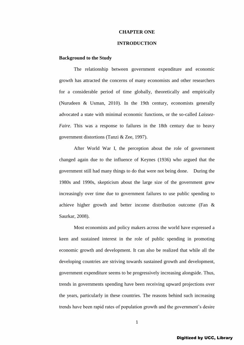
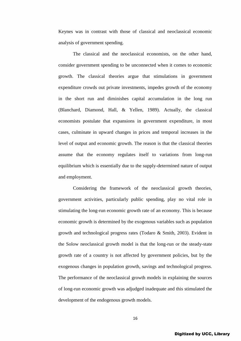
Figure 1 shows the trend of real GDP for Ghana for the period 1984 to 2015.

Figure 1: Trend of Real GDP

Source: World Bank (2014)

It can be observed from Figure 1 that Real GDP rises steadily from the

first quarter of 1984 through to the first quarter of 2014 and thereafter falls

19.5

20

20.5

21

21.5

22

22.5

23

19

84

q1

19

85

q4

19

87

q3

19

89

q2

19

91

q1

19

92

q4

19

94

q3

19

96

q2

19

98

q1

19

99

q4

20

01

q3

20

03

q2

20

05

q1

20

06

q4

20

08

q3

20

10

q2

20

12

q1

20

13

q4

20

15

q3

Real GDP


5

sharply. This means that real GDP has seen a consistent improvement over the

years until 2014 where it suddenly deteriorated.

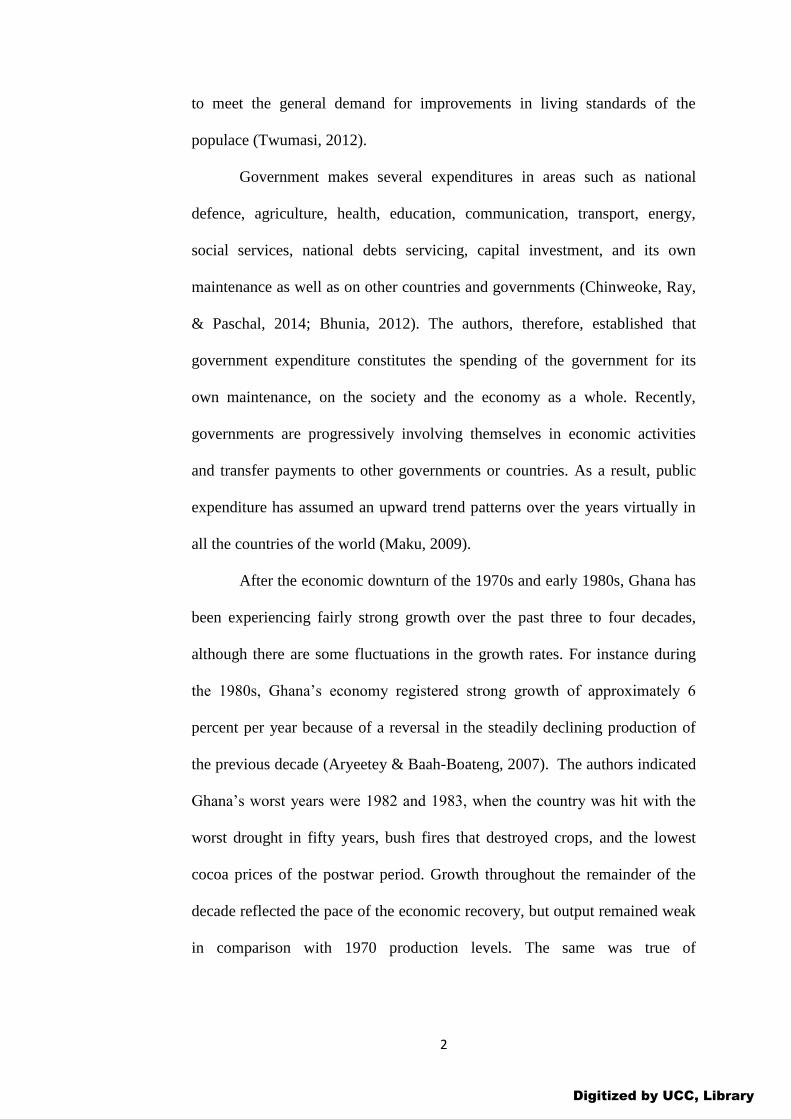
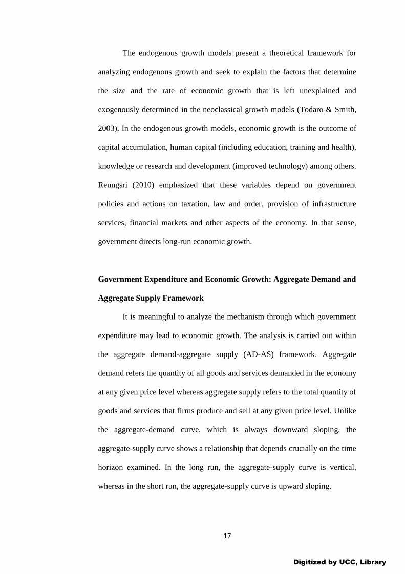
Figure 2 highlights the trend of government interest payment for from 1984 to

2015.

Figure 2: Trend of Government Interest Payment


It can be inferred from Figure 2 that, government interest payment has

been very unstable, i.e. it has been fluctuating consistently over the study

period. From 1985 second quarter, it increased significantly until the first

quarter of 1989. Thereafter, the country experienced alternate rise and fall in

interest payment. There was an astronomic rise and fall between 2006 and

2010. It increased afterwards and drops marginally in 2011 quarter 3 before

rising and a sharp fall from 2014 quarter 1.

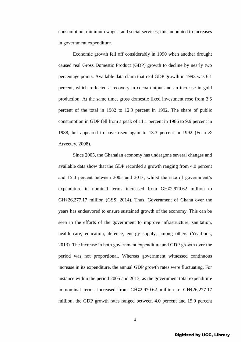
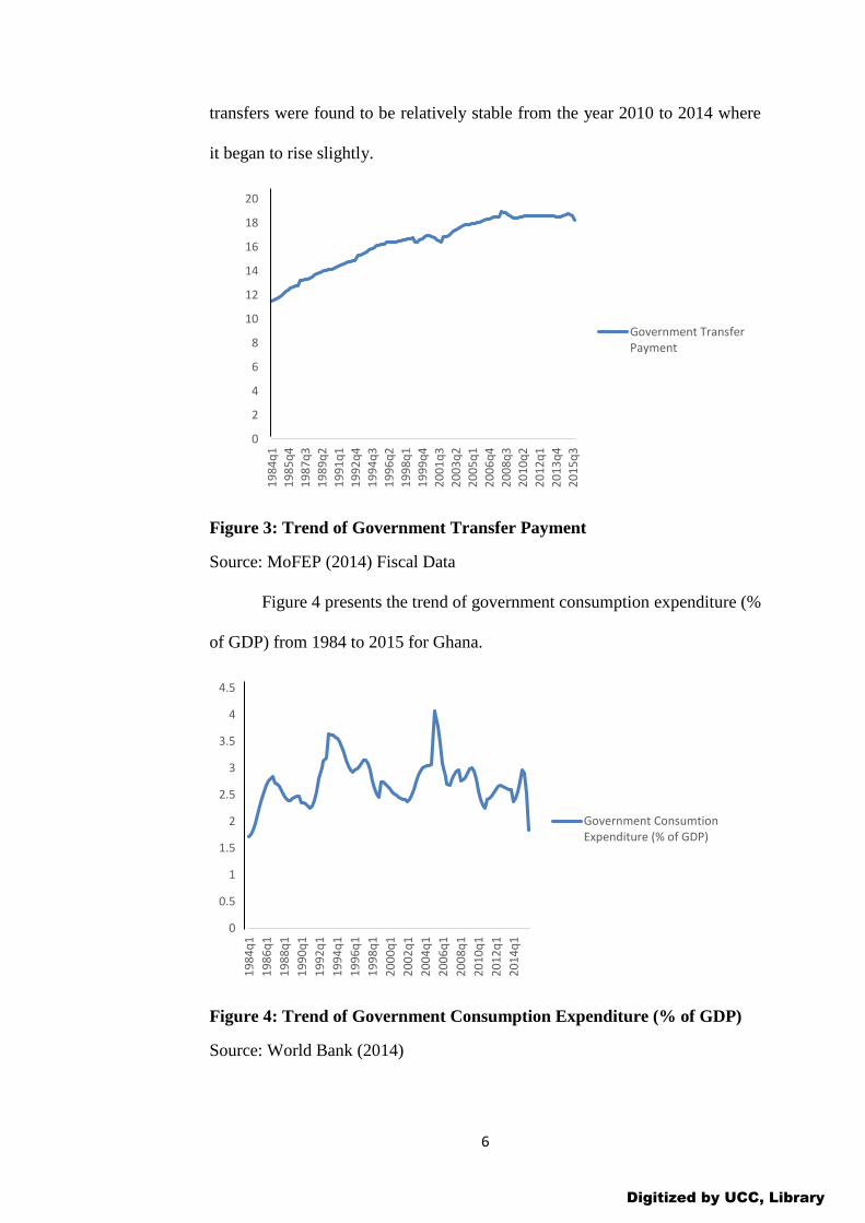
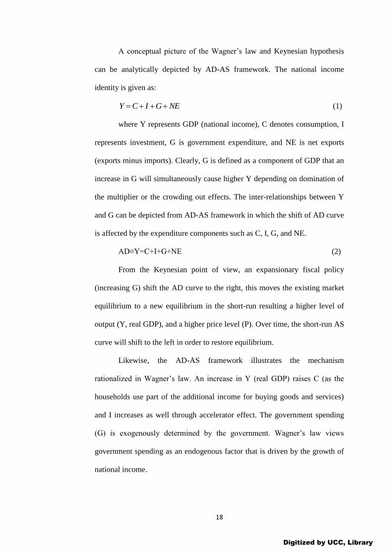
Figure 3 depicts the trend of government transfer payment for Ghana

for the period 1984 to 2015. From Figure 3, it be seen that government

transfer payment has been increasing consistently over the study period.

Around late 1990s and early 2000, the country witnessed some rise and fall in

transfer payment although such fluctuations are not significant. However,

14.5

15

15.5

16

16.5

17

17.5

181

98

4q

1

19

86

q1

19

88

q1

19

90

q1

19

92

q1

19

94

q1

19

96

q1

19

98

q1

20

00

q1

20

02

q1

20

04

q1

20

06

q1

20

08

q1

20

10

q1

20

12

q1

20

14

q1

Government InterestPayment


6

transfers were found to be relatively stable from the year 2010 to 2014 where

it began to rise slightly.

Figure 3: Trend of Government Transfer Payment

Source: MoFEP (2014) Fiscal Data

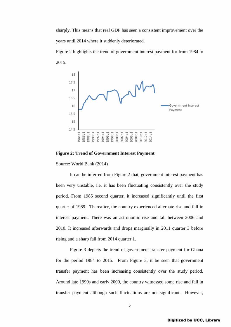
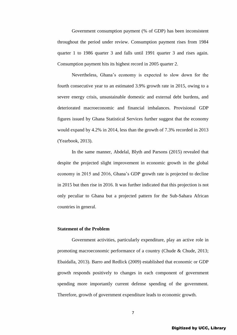
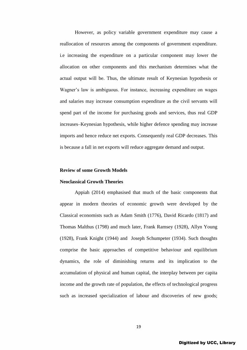
Figure 4 presents the trend of government consumption expenditure (%

of GDP) from 1984 to 2015 for Ghana.

Figure 4: Trend of Government Consumption Expenditure (% of GDP)


0

2

4

6

8

10

12

14

16

18

20

19

84

q1

19

85

q4

19

87

q3

19

89

q2

19

91

q1

19

92

q4

19

94

q3

19

96

q2

19

98

q1

19

99

q4

20

01

q3

20

03

q2

20

05

q1

20

06

q4

20

08

q3

20

10

q2

20

12

q1

20

13

q4

20

15

q3

Government TransferPayment

0

0.5

1

1.5

2

2.5

3

3.5

4

4.5

19

84

q1

19

86

q1

19

88

q1

19

90

q1

19

92

q1

19

94

q1

19

96

q1

19

98

q1

20

00

q1

20

02

q1

20

04

q1

20

06

q1

20

08

q1

20

10

q1

20

12

q1

20

14

q1

Government ConsumtionExpenditure (% of GDP)


7

Government consumption payment (% of GDP) has been inconsistent

throughout the period under review. Consumption payment rises from 1984

quarter 1 to 1986 quarter 3 and falls until 1991 quarter 3 and rises again.

Consumption payment hits its highest record in 2005 quarter 2.

Nevertheless, Ghana’s economy is expected to slow down for the

fourth consecutive year to an estimated 3.9% growth rate in 2015, owing to a

severe energy crisis, unsustainable domestic and external debt burdens, and

deteriorated macroeconomic and financial imbalances. Provisional GDP

figures issued by Ghana Statistical Services further suggest that the economy

would expand by 4.2% in 2014, less than the growth of 7.3% recorded in 2013

(Yearbook, 2013).

In the same manner, Abdelal, Blyth and Parsons (2015) revealed that

despite the projected slight improvement in economic growth in the global

economy in 2015 and 2016, Ghana’s GDP growth rate is projected to decline

in 2015 but then rise in 2016. It was further indicated that this projection is not

only peculiar to Ghana but a projected pattern for the Sub-Sahara African

countries in general.

Statement of the Problem

Government activities, particularly expenditure, play an active role in

promoting macroeconomic performance of a country (Chude & Chude, 2013;

Ebaidalla, 2013). Barro and Redlick (2009) established that economic or GDP

growth responds positively to changes in each component of government

spending more importantly current defense spending of the government.

Therefore, growth of government expenditure leads to economic growth.


8

Accordingly, many empirical studies including Aregbeyen (2006);

Ebaidalla (2013); Kamasa and Ofori-Abebrese (2015) have focused on the

relationship between government expenditure and economic growth. The

debate on the topic is ongoing with diverse focus. While Ebaidalla (2013)

indicated that government expenditure influences economic growth positively,

Appiah (2014), and Kamasa and Ofori-Abebrese (2015) highlighted that

economic growth drives government expenditure growth in Ghana. Saiyed

(2012) asserted that both government expenditure and economic growth

influence each other in India.

Thus, all these findings failed to reach a definite answer for the

question of direction of causality between the two variables. In other words,

some empirical results confirm the Wagner view rather than the Keynesian

hypothesis, while other findings advocate the Keynesian view. Such

differences in the results on the connection between government expenditure

and economic growth can be attributed to different specifications, different

sample periods, and data from different countries.

According to the Keynesian perspective, government policy could

reverse economic recession via various government spending programmes

such as infrastructural development. Keynes (1936) is of the view that

increased government consumption has a high potential of increasing

employment, profitability and investment through its multiplier effects on

aggregate demand. Hence, economic growth can be influenced positively by

government expenditure, both recurrent and capital expenditures. But,

endogenous growth models predict that only those productive government


9

expenditure components will positively affect the long run growth rate (Barro,

1990).

However, Wagner’s hypothesis presupposes that government

expenditure has no impact on growth of the economic, but rather economic

growth impacts government spending positively. For instance, Yackovlev,

Lledo and Gadenne (2009) established that government expenditure growth is

the outcome of economic growth in sub-Saharan African and other developing

countries.

Fan and Saurkar (2008) studied trends of government spending in

developing countries. Their results indicated that in Africa and Asia,

government expenditures in agriculture and education were particularly robust

in promoting economic growth, but in Latin America, spending in agriculture,

infrastructure and social security had positive growth-promoting effects. Their

results further revealed that Structural Adjustment Programmes (SAPs) had a

negative effect on growth in Africa, but no statistically significant effects in

Asia and Latin America. Moreover, Saad and Kalakech (2009) indicated that

public expenditure on education has positive effect on economic growth only

in the long-run but not in the short run. Hence, various types of government

spending have differential impacts on economic growth. However, their

findings contradict with the works of Landau (1986); Devarajan, Swaroop and

Zou (1996); Miller and Russek (1997) who found insignificant positive

relationship between public expenditure on education and economic growth of

developing economies.

In Ghana, well-known empirical studies in this area include Kamasa

and Ofori-Abebrese (2015), Appiah, (2014); Twumasi (2012); and Nketiah-


10

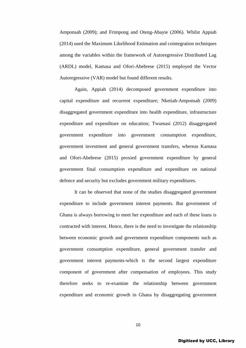
Amponsah (2009); and Frimpong and Oteng-Abayie (2006). Whilst Appiah

(2014) used the Maximum Likelihood Estimation and cointegration techniques

among the variables within the framework of Autoregressive Distributed Lag

(ARDL) model, Kamasa and Ofori-Abebrese (2015) employed the Vector

Autoregressive (VAR) model but found different results.

Again, Appiah (2014) decomposed government expenditure into

capital expenditure and recurrent expenditure; Nketiah-Amponsah (2009)

disaggregated government expenditure into health expenditure, infrastructure

expenditure and expenditure on education; Twumasi (2012) disaggregated

government expenditure into government consumption expenditure,

government investment and general government transfers, whereas Kamasa

and Ofori-Abebrese (2015) proxied government expenditure by general

government final consumption expenditure and expenditure on national

defence and security but excludes government military expenditures.

It can be observed that none of the studies disaggregated government

expenditure to include government interest payments. But government of

Ghana is always borrowing to meet her expenditure and each of these loans is

contracted with interest. Hence, there is the need to investigate the relationship

between economic growth and government expenditure components such as

government consumption expenditure, general government transfer and

government interest payments-which is the second largest expenditure

component of government after compensation of employees. This study

therefore seeks to re-examine the relationship between government

expenditure and economic growth in Ghana by disaggregating government


11

expenditure to capture government consumption expenditure, general

government transfers and government interest payments.

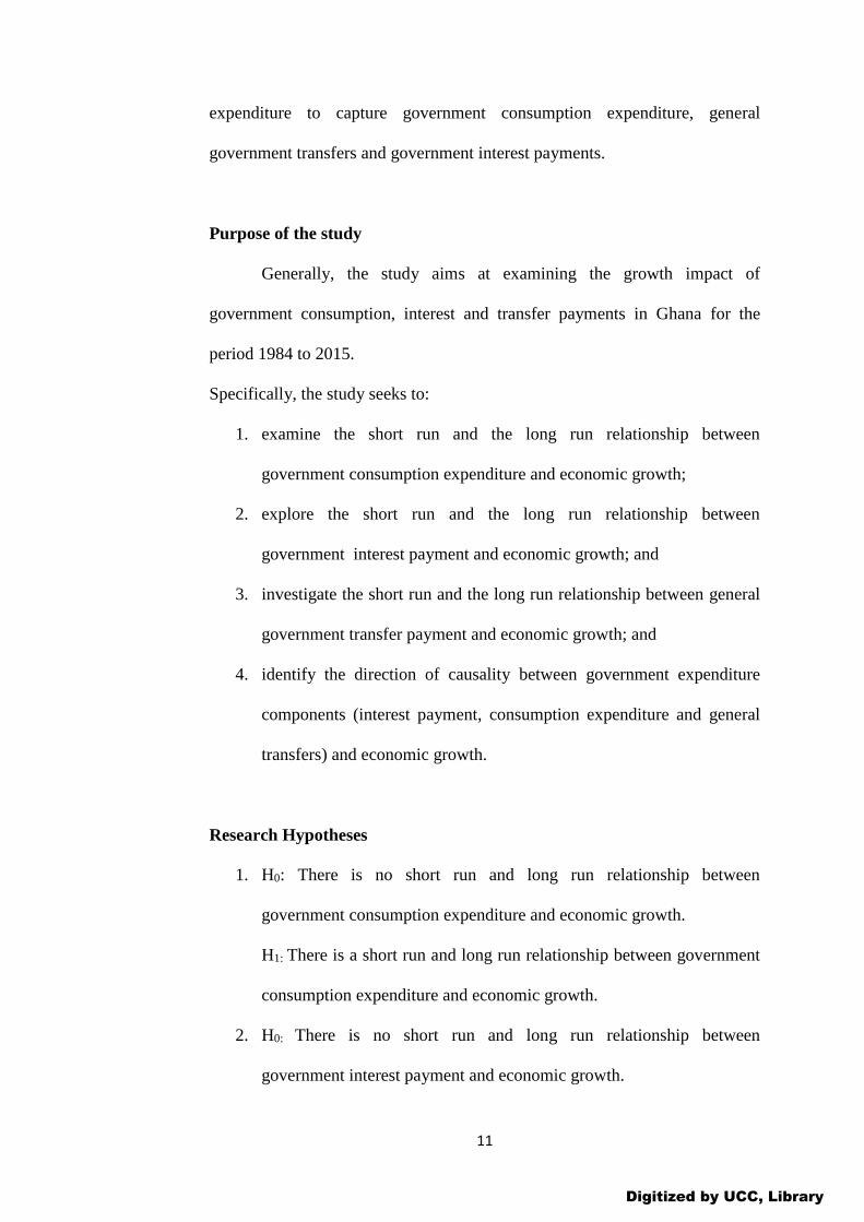
Purpose of the study

Generally, the study aims at examining the growth impact of

government consumption, interest and transfer payments in Ghana for the

period 1984 to 2015.

Specifically, the study seeks to:

1. examine the short run and the long run relationship between

government consumption expenditure and economic growth;

2. explore the short run and the long run relationship between

government interest payment and economic growth; and

3. investigate the short run and the long run relationship between general

government transfer payment and economic growth; and

4. identify the direction of causality between government expenditure

components (interest payment, consumption expenditure and general

transfers) and economic growth.

Research Hypotheses

1. H0: There is no short run and long run relationship between

government consumption expenditure and economic growth.

H1: There is a short run and long run relationship between government

consumption expenditure and economic growth.

2. H0: There is no short run and long run relationship between

government interest payment and economic growth.


12

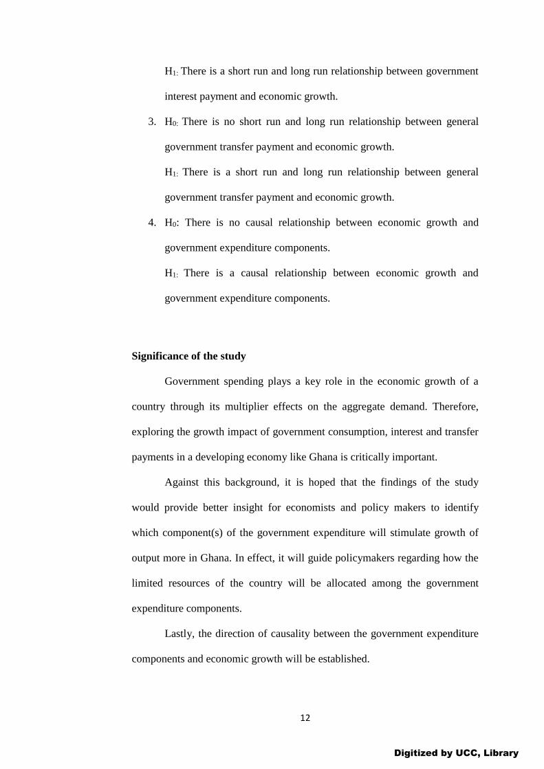
H1: There is a short run and long run relationship between government

interest payment and economic growth.

3. H0: There is no short run and long run relationship between general

government transfer payment and economic growth.

H1: There is a short run and long run relationship between general

government transfer payment and economic growth.

4. H0: There is no causal relationship between economic growth and

government expenditure components.

H1: There is a causal relationship between economic growth and

government expenditure components.

Significance of the study

Government spending plays a key role in the economic growth of a

country through its multiplier effects on the aggregate demand. Therefore,

exploring the growth impact of government consumption, interest and transfer

payments in a developing economy like Ghana is critically important.

Against this background, it is hoped that the findings of the study

would provide better insight for economists and policy makers to identify

which component(s) of the government expenditure will stimulate growth of

output more in Ghana. In effect, it will guide policymakers regarding how the

limited resources of the country will be allocated among the government

expenditure components.

Lastly, the direction of causality between the government expenditure

components and economic growth will be established.


13

Scope of the study

This study aimed to critically examine the growth impact of

government consumption, interest and transfer payments in Ghana. A

quarterly time series dataset for the period 1984 to 2015 was used. The study

employed the Autoregressive Distributed Lag (ARDL) model otherwise

known as the bounds testing approach to cointegration developed by Pesaran

and Shin (1998); Pesaran, Shin and Smith (2001).

Organization of the study

The study is organized under five chapters. Chapter one comprises the

background to the study, statement of the problem, objectives of the study,

research hypotheses, significance of the study, scope and organization of the

study. The chapter two presents the review of related literature covering both

theoretical and empirical review. Chapter three will discuss the methodology

adopted for the study. Specifically, it highlights the research design,

theoretical and empirical model specifications as well as description and

sources of data. Chapter four covers results and discussion. The final chapter,

five summarizes the main findings of the study, discusses the policy

implications and recommendations for economists and policy makers in

Ghana, and finally acknowledges the limitations of the study.


14

CHAPTER TWO

REVIEW OF RELATED LITERATURE

Introduction

This chapter is devoted to the review of literature related to

government expenditure and economic growth nexus. The chapter is organized

under three main sections–one, theoretical literature review; two, review of

trend of government expenditure and economic growth in Ghana; and three,

empirical literature review.

Theoretical Literature Review

This section of the literature review focuses on the review of the

theoretical background of government expenditure and economic growth

nexus, some theories of economic growth with specific emphasis on the

neoclassical (Solow-Swan, Peacock-Shaw) growth model, and endogenous

growth model including Afonso-Alegre growth theory, the role of the

government in economic growth, and some theories of government

expenditure growth.

Theoretical Background of Government Expenditure and Economic

Growth Nexus

The relationship between public expenditure and economic growth has

been extensively researched and has been an issue which has attracted

considerable debate among the various economic schools of thought including

Keynes. Oyinlola and Akinnibosun (2013) indicated that, the theoretical

underpinning of this relationship can be traced to the time of Wagner (1883) to


15

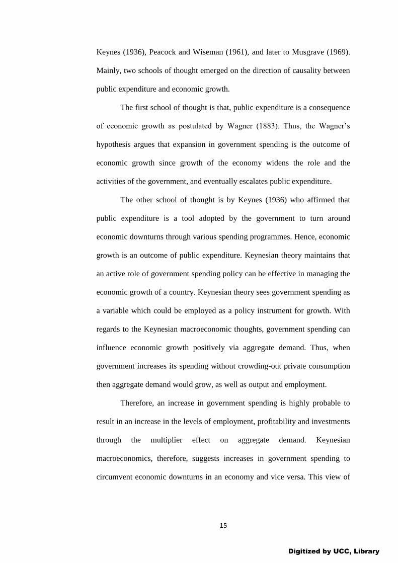
Keynes (1936), Peacock and Wiseman (1961), and later to Musgrave (1969).

Mainly, two schools of thought emerged on the direction of causality between

public expenditure and economic growth.

The first school of thought is that, public expenditure is a consequence

of economic growth as postulated by Wagner (1883). Thus, the Wagner’s

hypothesis argues that expansion in government spending is the outcome of

economic growth since growth of the economy widens the role and the

activities of the government, and eventually escalates public expenditure.

The other school of thought is by Keynes (1936) who affirmed that

public expenditure is a tool adopted by the government to turn around

economic downturns through various spending programmes. Hence, economic

growth is an outcome of public expenditure. Keynesian theory maintains that

an active role of government spending policy can be effective in managing the

economic growth of a country. Keynesian theory sees government spending as

a variable which could be employed as a policy instrument for growth. With

regards to the Keynesian macroeconomic thoughts, government spending can

influence economic growth positively via aggregate demand. Thus, when

government increases its spending without crowding-out private consumption

then aggregate demand would grow, as well as output and employment.

Therefore, an increase in government spending is highly probable to

result in an increase in the levels of employment, profitability and investments

through the multiplier effect on aggregate demand. Keynesian

macroeconomics, therefore, suggests increases in government spending to

circumvent economic downturns in an economy and vice versa. This view of


16

Keynes was in contrast with those of classical and neoclassical economic

analysis of government spending.

The classical and the neoclassical economists, on the other hand,

consider government spending to be unconnected when it comes to economic

growth. The classical theories argue that stimulations in government

expenditure crowds out private investments, impedes growth of the economy

in the short run and diminishes capital accumulation in the long run

(Blanchard, Diamond, Hall, & Yellen, 1989). Actually, the classical

economists postulate that expansions in government expenditure, in most

cases, culminate in upward changes in prices and temporal increases in the

level of output and economic growth. The reason is that the classical theories

assume that the economy regulates itself to variations from long-run

equilibrium which is essentially due to the supply-determined nature of output

and employment.

Considering the framework of the neoclassical growth theories,

government activities, particularly public spending, play no vital role in

stimulating the long-run economic growth rate of an economy. This is because

economic growth is determined by the exogenous variables such as population

growth and technological progress rates (Todaro & Smith, 2003). Evident in

the Solow neoclassical growth model is that the long-run or the steady-state

growth rate of a country is not affected by government policies, but by the

exogenous changes in population growth, savings and technological progress.

The performance of the neoclassical growth models in explaining the sources

of long-run economic growth was adjudged inadequate and this stimulated the

development of the endogenous growth models.


17

The endogenous growth models present a theoretical framework for

analyzing endogenous growth and seek to explain the factors that determine

the size and the rate of economic growth that is left unexplained and

exogenously determined in the neoclassical growth models (Todaro & Smith,

2003). In the endogenous growth models, economic growth is the outcome of

capital accumulation, human capital (including education, training and health),

knowledge or research and development (improved technology) among others.

Reungsri (2010) emphasized that these variables depend on government

policies and actions on taxation, law and order, provision of infrastructure

services, financial markets and other aspects of the economy. In that sense,

government directs long-run economic growth.

Government Expenditure and Economic Growth: Aggregate Demand and

Aggregate Supply Framework

It is meaningful to analyze the mechanism through which government

expenditure may lead to economic growth. The analysis is carried out within

the aggregate demand-aggregate supply (AD-AS) framework. Aggregate

demand refers the quantity of all goods and services demanded in the economy

at any given price level whereas aggregate supply refers to the total quantity of

goods and services that firms produce and sell at any given price level. Unlike

the aggregate-demand curve, which is always downward sloping, the

aggregate-supply curve shows a relationship that depends crucially on the time

horizon examined. In the long run, the aggregate-supply curve is vertical,

whereas in the short run, the aggregate-supply curve is upward sloping.


18

A conceptual picture of the Wagner’s law and Keynesian hypothesis

can be analytically depicted by AD-AS framework. The national income

identity is given as:

Y C I G NE (1)

where Y represents GDP (national income), C denotes consumption, I

represents investment, G is government expenditure, and NE is net exports

(exports minus imports). Clearly, G is defined as a component of GDP that an

increase in G will simultaneously cause higher Y depending on domination of

the multiplier or the crowding out effects. The inter-relationships between Y

and G can be depicted from AD-AS framework in which the shift of AD curve

is affected by the expenditure components such as C, I, G, and NE.

AD≡Y=C+I+G+NE (2)

From the Keynesian point of view, an expansionary fiscal policy

(increasing G) shift the AD curve to the right, this moves the existing market

equilibrium to a new equilibrium in the short-run resulting a higher level of

output (Y, real GDP), and a higher price level (P). Over time, the short-run AS

curve will shift to the left in order to restore equilibrium.

Likewise, the AD-AS framework illustrates the mechanism

rationalized in Wagner’s law. An increase in Y (real GDP) raises C (as the

households use part of the additional income for buying goods and services)

and I increases as well through accelerator effect. The government spending

(G) is exogenously determined by the government. Wagner’s law views

government spending as an endogenous factor that is driven by the growth of

national income.


19

However, as policy variable government expenditure may cause a

reallocation of resources among the components of government expenditure.

i.e increasing the expenditure on a particular component may lower the

allocation on other components and this mechanism determines what the

actual output will be. Thus, the ultimate result of Keynesian hypothesis or

Wagner’s law is ambiguous. For instance, increasing expenditure on wages

and salaries may increase consumption expenditure as the civil servants will

spend part of the income for purchasing goods and services, thus real GDP

increases–Keynesian hypothesis, while higher defence spending may increase

imports and hence reduce net exports. Consequently real GDP decreases. This

is because a fall in net exports will reduce aggregate demand and output.

Review of some Growth Models

Neoclassical Growth Theories

Appiah (2014) emphasised that much of the basic components that

appear in modern theories of economic growth were developed by the

Classical economists such as Adam Smith (1776), David Ricardo (1817) and

Thomas Malthus (1798) and much later, Frank Ramsey (1928), Allyn Young

(1928), Frank Knight (1944) and Joseph Schumpeter (1934). Such thoughts

comprise the basic approaches of competitive behaviour and equilibrium

dynamics, the role of diminishing returns and its implication to the

accumulation of physical and human capital, the interplay between per capita

income and the growth rate of population, the effects of technological progress

such as increased specialization of labour and discoveries of new goods;


20

methods of production and lastly, the role of monopoly power as an incentive

for technological advance.

Neoclassical theory was purposefully micro-oriented with much

emphasis on the utility-maximizing behaviour of individuals and the profit-

maximizing actions of perfectly competitive firms. The macroeconomic

perspective inherent in a concern for economic growth and in the distribution

of income among classes that had motivated the classical economists gave

way to a narrower interest in the conditions required for equilibrium prices and

quantities in individual markets.

Sequentially, the modern growth theory began with the classic work of

Ramsey (1928). From Ramsey (1928) through to the late 1950s, Harrod

(1939) and Domar (1946) (popularly known today as the Harrod-Domar

model) attempted to integrate Keynesian analysis with essentials of economic

growth. This model employed production functions with little substitutability

among the inputs and maintain that the free-market system is naturally

unstable. Their opinions were embraced compassionately by many economists

during the time in the sense that they wrote shortly after the Great Depression.

Despite the fact that very little of this analysis plays a role in our thinking

today, their contributions generated a lot of research at the time.

Peacock-Shaw (1971) Model

Peacock and Shaw (1971) demonstrated how fiscal policy affects

economic growth in their effort to extend the Harrod-Domar growth model.

The Peacock-Shaw model assumes that on the supply side output capacity c

tY


21

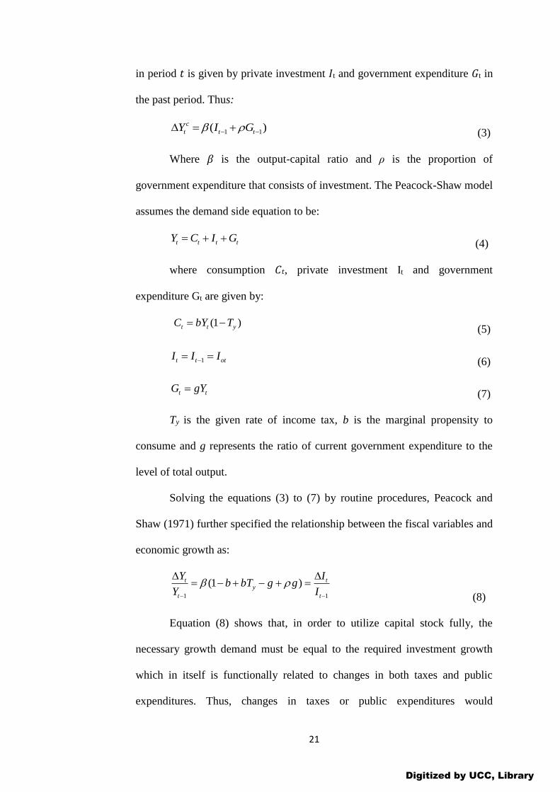
in period 𝑡 is given by private investment 𝐼t and government expenditure 𝐺t in

the past period. Thus:

1 1( )c

t t tY I G (3)

Where 𝛽 is the output-capital ratio and ρ is the proportion of

government expenditure that consists of investment. The Peacock-Shaw model

assumes the demand side equation to be:

t t t tY C I G (4)

where consumption 𝐶𝑡, private investment It and government

expenditure Gt are given by:

(1 )t t yC bY T

(5)

1t t otI I I (6)

t tG gY (7)

Ty is the given rate of income tax, b is the marginal propensity to

consume and g represents the ratio of current government expenditure to the

level of total output.

Solving the equations (3) to (7) by routine procedures, Peacock and

Shaw (1971) further specified the relationship between the fiscal variables and

economic growth as:

1 1

(1 )t ty

t t

Y Ib bT g g

Y I

(8)

Equation (8) shows that, in order to utilize capital stock fully, the

necessary growth demand must be equal to the required investment growth

which in itself is functionally related to changes in both taxes and public

expenditures. Thus, changes in taxes or public expenditures would


22

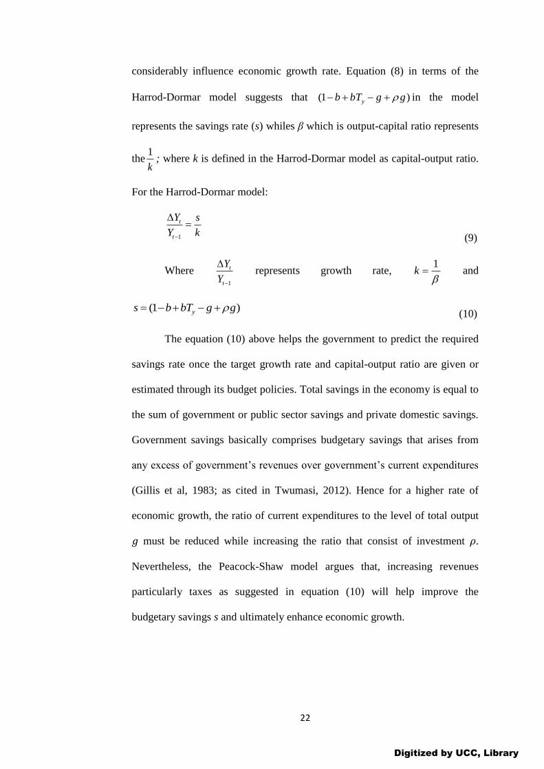
considerably influence economic growth rate. Equation (8) in terms of the

Harrod-Dormar model suggests that (1 )yb bT g g in the model

represents the savings rate (s) whiles β which is output-capital ratio represents

the1

k; where k is defined in the Harrod-Dormar model as capital-output ratio.

For the Harrod-Dormar model:

1

t

t

Y s

Y k

(9)

Where 1

t

t

Y

Y

represents growth rate,

1k

and

(1 )ys b bT g g (10)

The equation (10) above helps the government to predict the required

savings rate once the target growth rate and capital-output ratio are given or

estimated through its budget policies. Total savings in the economy is equal to

the sum of government or public sector savings and private domestic savings.

Government savings basically comprises budgetary savings that arises from

any excess of government’s revenues over government’s current expenditures

(Gillis et al, 1983; as cited in Twumasi, 2012). Hence for a higher rate of

economic growth, the ratio of current expenditures to the level of total output

𝑔 must be reduced while increasing the ratio that consist of investment 𝜌.

Nevertheless, the Peacock-Shaw model argues that, increasing revenues

particularly taxes as suggested in equation (10) will help improve the

budgetary savings s and ultimately enhance economic growth.


23

Solow (1956) Model

A typical illustration of the neoclassical ideology on growth was

developed by Solow (1956) and Swan (1956). This model is referred to as

Solow or Solow-Swan model and made more important contributions to

growth theories. The model was formulated by expanding the Harrod-Dormar

model to include labour and technology which the authors assumed to be an

independent variable to the growth equation (and that, its progress is

determined exogenously). In this model, Solow used a Cobb-Douglas

production function which is assumed to be characterized by constant returns

to scale. Thus, the key aspect of the Solow model is the neoclassical form of

the production function, a specification that assumes constant returns to scale,

diminishing returns to each input, and some positive and smooth elasticity of

substitution between the inputs. This production function is combined with a

constant saving rate rule to generate an extremely simple general equilibrium

model of the economy.

Solow (1956) believes that if production activity takes place under

neoclassical production conditions of variable proportions and constant returns

to scale, then there would be no resistance between natural and unwarranted

growth rates. The system is self-adjusting to any given rate of growth of

labour force and ultimately approaches a state of steady proportional

expansion. According to Van den Berg (2001), to make distinction between

the Solow and the Harrod-Domar growth models and its fixed capital-output

ratio, Solow specified a production function that allows factors to be

constantly substituted for each other. The implication of such constant

substitution is that, the marginal product of each factor is variable, and


24

depends on how much of the factor that is already used in production and how

many other factors it is combined with it.

The Solow growth model importantly assumed that each factor of

production is subject to diminishing returns. Moreover, the production

function suits the properties that: the marginal products of inputs get closer to

infinity as inputs are reduced to zero and approach zero as inputs are increased

infinitely. In fact the inherent weakness, in the Harrod-Domar model, that a

constant rate of saving and investment could bring perpetual economic growth

is evidently revealed by Solow model.

Accordingly, Solow argued that the reality of diminishing returns in

the production process and constant investment by itself could not generate

permanent growth of an economy, in the sense that diminishing returns would

eventually cause the gains in output from investment to approach zero.

Consequently, Solow (1956) contributed tremendously to the theory of

economic growth by laying emphasis on long-run growth. Solow again

hypothesized that long-run growth is in essence influenced by technological

change and not by savings or investment. They noted that saving only

determines short-run growth of the economy, since the economy will run into

diminishing returns as the ratio of capital per labour increases. In response to

this, Perman and Stern (2003) indicated that the absence of constant

improvement in technology, per capita growth will eventually cease and vice

versa.

Solow’s model primarily assumes that, economic growth is the

outcome of the combination of capital and labour. As a result, the following

question emerged: how much of output growth can be attributed to other


25

factors of production apart from labour and capital? In order to address the

question, Solow classified the growth in output into three components, each

identifiable as contribution of one factor of production, that is labour, capital,

and total factor productivity. This implied that in the Solow model, long term

economic growth is explained by labour augmenting technological change and

by the increase of capital per labour.

The total factor productivity (TFP) is usually termed as the Solow

residual. The term residual is appropriate, because the estimate denotes the

part of measured GDP growth that may not be explained by labour and capital.

The residual refers to the difference between the rate of growth of output and

the weighted average of the rates of growth of capital and labour, with factor

income shares as weights. The TFP is calculated under the assumption of

perfect competition in the labour and capital market as well as the product and

service markets.

Endogenous Growth Models

In the late 1980s, quite a lot of models of endogenous growth began to

emerge in the economics literature and as a result, economic growth theory

experienced a remarkable revival and became once more a very active area of

macroeconomic research. According to D’Agata and Freni (2003), the goal of

the endogenous growth theory was twofold: one was to rise above the

shortfalls of the Solow and Ramsey models which failed to address persistent

growth; and lastly, was to develop a more robust model in which all variables

- which matter for growth such as savings, investment, and technical

knowledge- are the outcome of rational decisions.


26

Unlike neoclassical growth theories, endogenous growth theories do

not assume that physical capital accumulation is the dominant factor that

mainly determines economic growth nor explains the differences in income

levels among nations. Again, Cypher and Dietz (2004) maintain that the

endogenous models failed to accept the neoclassical and classical assumption

of diminishing returns as applying to any of the reproducible inputs of

production such as capital and labour, but also technology, effectively turning

a nation’s short-run production function into a long-run, dynamic relationship

that can be constantly evolving. Although diminishing returns operates in any

production process, the introduction of high pace of technological progress has

claimed superiority over it in the long run. This means that the classical and

neoclassical economists did not take into consideration the relationship

between technological progress and the phenomena of diminishing returns.

Endogenous growth models maintain that a higher level of investment

may not only increase per capita income, as the neoclassical models say, but

also higher investment rates can generate greater rates of growth of per capita

income in the future.

This is, however, not possible within the conventional neoclassical

growth model, which posits that a steady-state income level, determined by

the rate of saving and the population growth rate, is the equilibrium outcome

of the growth process. Given that population growth is a constant, higher

levels of income simply are not attainable in the neoclassical model without

either an increase in the rate of saving or an exogenous advancement in the

level of technology. The endogenous growth models hold different view with

respect to this. These models argue that it is possible for countries to continue


27

to grow rapidly for long periods, even when they already have achieved

relatively high incomes. This sustaining of growth rates can occur without an

increase in the rate of savings.

Cypher and Dietz (2004) highlight that when the link between the rate

of economic growth and the law of diminishing returns is suppressed, and the

ceiling on income per person for any particular rate of savings and investment

is eliminated, endogenous growth models can easily elucidate the existence of

widening income gap between poorer and richer countries.

In most endogenous growth models, one of the most important factors

of production contributing to higher and continuous growth has been found to

be both the rate of accumulation, as well as the initial stock, of human capital.

While these models share some similarities with the capital and saving-

centered neoclassical growth models in their form, the endogenous growth

models do not envisage the convergence of income levels, even among

countries with similar rates of saving, investment and population growth rates.

Indeed, these models demonstrate how it is possible for some countries

to continue to grow faster than others far into the future, with both the absolute

and relative income gap growing. Endogenous growth models in addition lay a

diverse emphasis on what is required to enhance a nation’s economic growth

and development possibilities compared to the recommendations derived from

the capital-and saving-centered neoclassical-type models.

It must be noted at this point that, the foremost conceptual disparity

between the Solow’s neoclassical growth models and the endogenous growth

models is that the endogenous models do not assume any diminishing returns

to the reproducible inputs, K - the stock of physical capital, to H - the stock of


28

human capital or to technology. Rather it is presumed that constant, or even

increasing marginal returns are possible. The endogenous growth models

assume that, there are likely to be significant positive externalities to human

capital accumulation and, possibly to some physical capital accumulation to

the degree that new capital embodies new technology, so that the classical and

neoclassical result of diminishing returns to K and H are avoided through such

society-wide spill-over effects.

When the social benefits from human capital accumulation exceed the

private benefits, there will be positive secondary and tertiary effects from, say,

an increase in a country’s average education level or enrollment ratios that

reverberate through the economy.

More educated and presumably more productive workers not only

produce more at their own tasks, but they also interact synergistically with

their workmates so that the productivity of other workers also rises, even

though their level of education may have remained unchanged. Higher average

levels of education among a population also can contribute to learning-by-

doing effects. That is, the capacity of labour to build upon its past education

and training, so that the same level of human capital input actually is able to

improve its productivity over time in the process of producing goods and

services on the shop floor, or wherever production takes place.

Learning-by-doing contributes to increases in the potential level of

total output without the need for an increase in any additional inputs and with

no increase in investment. Learning-by-doing effects increase the productivity

and effectiveness of labour. The presumption is that the higher the level of

human capital accumulation in an economy, the stronger will be such effects,


29

again breaking the link between growth in labour and human capital

accumulation and diminishing returns.

Based on the endogenous growth theory, the ability to use technology,

the ability to develop it and the skills of the labour force available to

complement technological knowledge are all formed in and shaped by each

particular economy. In other words, growth is an endogenous process, coming

from within each particular economy, with each having a different production

function indicating diverse quantities and qualities of its inputs.

Afonso-Alegre (2008) Growth Model

Afonso-Alegre’s growth model expanded a simple endogenous growth

model to demonstrate the system through which the different types of public

expenditures and taxes affect economic growth. The model assumes an

economy with four types of public expenditures and three types of taxes in an

extended Cobb-Douglas type model with constant returns to scale. The types

of the public expenditures in the model are: the expenditures on public input in

the production function (𝐺1); the capital-enhancing type of public expenditure

(𝐺2); the labour-enhancing type public expenditure (𝐺3) and; the publicly

provided consumption good (𝐺4). Tax components comprise taxes on

consumption (𝜏𝑐), taxes on corporate profits (𝜏𝜋) and taxes on labour income

(𝜏𝑙). The production function can be written as:

1, t t t tY AK L G

(11)


30

where Kt and Lt denote private capital and labour supply respectively

and 𝐺1denotes the public input in production which is taken as a separate input

in the production function. For simplicity, the capital-enhancing type

expenditure 𝐺2 is assumed to be a subsidy to the purchase of private capital

(Deverajan et al. 1996; Afonso & Alegre, 2008; Twumasi, 2012). The

subsidized private capital paid through the capital-enhancing type of public

expenditure is assumed be to be given by:

2, (1 )t t tG s K (12)

Based on the theory that 𝐺2 provides an incentive to private investment

and where 1-st is the subsidized share of private capital.

Assuming a labour supply that depends on the level of government

expenditure on labour 𝐺3, the level of population growth 𝑁𝑡 and the

equilibrium real wage w:

3,t t t tL w G N (13)

The parameters µ and ŋ are assumed to lie in the interval (0,1) but νis

accepted to be between -1 and 1 since public policies that create disincentives

to labour supply on the labour market can exist (Afonso & Alegre, 2008;

Twumasi, 2012).

Assuming further a Cobb-Douglas type utility function for the

household agent(s) who live for an infinite number of years, the utility

function is considered as:

(1 )

4,

t

j t t

t j

U C G

(14)

Where 𝐶t represents household consumption, 𝐺4 represents the public

type of spending that is directly consumed by households and therefore


31

entering the utility function as 𝐺4. Average consumption for household agents

as in line with economic theory is assumed not to change during their life time

but there can be temporal fluctuations.

The household agents are considered to be the owners of capital and

firms, and supplies labour. For the budget constraint, the household agent will

have to choose the share of their income that they want to consume or invest

in additional capital for the next period and in addition pay taxes on labour, on

corporate profits and on consumption. The household’s constraint can be

shown as:

1 1(1 ) (1 ) (1 )C t t t l t t t tC s K wL r K (15)

where C , l and are the previously defined tax types, t and tr

represent corporate profits and the equilibrium rate price of capital paid by

firms to households respectively. Also, household agents are assumed to take

the decisions of the government concerning taxes and public expenditures as

exogenous and also decide on their own how to distribute their income

between private capital investment and current consumption. The household

agents consume to maximize their utility (14) subject to the budget constraint

(15). When we log-linearise and substitute the equations for labour and capital

in (11), the effect of permanent increases in any of the proposed fiscal

variables can further be specified in the form of growth as:

1

(1 )0t

t

y

g

(16)

2

(1 )(1 )0t t

t

y s

g s

(17)


32

3

0t

t

y

g

(18)

4

(1 )(1 )0t

t

y

g

(19)

Where (1 )(1 ) and the elements represented by small

letters denote their growth rates. And in much the same way, that of taxes can

also be shown as:

, ,

(1 )0

(1 ) (1 )

t

t t

y

(20)

,

(1 )0

(1 )

t

t

y

(21)

Where , ,(1 ) (1 )t t

The derivations above show that changes in the levels public input in

production (𝐺1), capital enhancing public-expenditure (𝐺2) and labour-

enhancing public expenditure (𝐺3) will all have permanent and positive effects

on growth whereas changes in both labour income tax (𝜏𝑙) and corporate

income tax (𝜏𝜋,𝑡) will also have permanent and negative effects on growth.

And since government expenditure on consumption 𝐺4 and consumption tax

(𝜏𝑐) affect the economy through consumption, both would affect growth

temporarily based on the theory that consumers would not change their

consumption pattern in the long run.

The Role of Government in Economic Growth

The Minimal Government Argument


33

Hindriks and Myle (2006) observe that the very basic motivation for

the existence of the government follows from the experience that an entirely

unregulated economic activity could not operate smoothly in a very

sophisticated way. Thus, an economy will not function effectively if there

were no property rights (the rules governing the ownership of property) or

contract laws (the rules defining the conduct of trade). The reason here is that

without property rights, satisfactory exchange of commodities could not

happen in the face of mistrust that would exist between contracting parties.

Property rights, therefore, ensure that the participants in a trade obtain what

they expect and if they are not satisfied, it opens an avenue to seek redress.

Examples of contract laws include the formalization of weights and measures

and the obligation to offer product warranties. These laws give confidence to

trade by checking some of the risks and uncertainties in transactions.

The minimal state argument can be traced back to Hobbes in the 17th

century, who perceived the government as a social contract that enabled

people to escape from the anarchic “state of nature” where their competition in

pursuit of self-interest would lead to a destructive “war of all against all”.

The authors, particularly Hindriks and Myles (2006), maintain that the

institution of property rights is the first step away from this anarchy but

property rights and contract laws are not sufficient in themselves. Unless they

can be regulated and upheld in law, they are of limited importance. However,

such law enforcement cannot be provided free of cost. Enforcement officers

must be employed and courts must be provided where redress can be sought.

In addition, a society would also face a need for the enforcement of more

general criminal laws. Moving beyond this, a country needs to defend it


34

territories against any external aggression. This implies the provision of

defence for the nation.

In sum, the minimal-state concern offers contract laws, supervises it

and protects the economy against any external hostility. This is exactly what

the minimal state does. However, without it any meaningful economic activity

cannot be achieved. This therefore justifies the need for a government

(Appiah, 2014).

The Market versus the Government

Hindriks and Myles (2006) are of the view that aside the essential

prerequisites for a well-structured economic activity, there are other instances

in which government interventions in the economy can meaningfully enhance

welfare. The situations where government intervention may be deemed

appropriate can be categorized into two: i.e those that are associated with

market failure and those that do not involve any market failure.

Leach (2004) believes that in the existence of market failure, the

argument for considering whether intervention would be beneficial is

compelling. Consider a situation where an economic activity produces

externalities (effects that one economic agent imposes on another without their

consent), so that there is a divergence between private and social costs and the

competitive outcome is not efficient, it will be indispensable for the

government to intervene to check the inefficiency that emanates from such

economic activity . The last argument can also be extended to other cases of

market failure, such as those connected to the existence of public goods and


35

imperfect competition. Hence government intervention in such market failures

on efficiency grounds justified.

It must however be emphasized at this point that this line of argument

does not imply that government intervention will always be necessarily

beneficial and welfare enhancing. In every case, it must be demonstrated that

the government actually has the ability to improve upon what the unregulated

economy can achieve. This cannot be achieved if the policy tool adopted is

limited or government information is restricted. It will also be undesirable if

the government is not benevolent. While some useful insights follow from the

assumption of an omnipotent, omniscient and benevolent policy maker, in

reality it can give us very misleading ideas about the possibilities of beneficial

policy intervention. It must be recognized that the actions of the government

and the feasible policies that it can choose are often restricted by the same

features of the economy that make the market outcome inefficient.

Moreover, Stiglitz (1989) emphasized that a government managed by

non-benevolent officials and subject to political constraints may fail to correct

these market failures and may instead introduce new costs for its own

operation. He added that it is imperative to appreciate the fact that this

potential for government failure is as important as market failure. Nonetheless,

the very power to coerce raises the possibility of its misuse (Stiglitz, Heertje,

& de Beaufort, 1989). Although the intention of creating this power is that its

force should serve the general interest, nothing can guarantee that once public

officials are given this monopoly power, they will not try to abuse this power

in their own interest (Hindriks & Myles, 2006).


36

Some Theories of Government Expenditure Growth

Musgrave and Rostow's Development Model

The basis of the development model of public expenditure growth is

that the economy develops; its structure and needs change over time.

Accordingly, by following the nature of the development process from the

beginning of industrialization through to the completion of the development

process, a story of why government expenditure rises can be told. Aladejare

(2013) highlights the stages of development as postulated by Musgrave and

Rostow to include the following:

The early phase of development is considered as the period of

industrialization during which the population moves from the countryside to

the urban areas. Therefore in order to meet the needs that result from this

movement, there is a requirement for a significant infrastructural expenditure

in the development of cities. The typically rapid growth experienced in this

stage of development results in a substantial increase in expenditure and the

dominant role of infrastructure determines the nature of expenditure.

During the middle stage of development, the infrastructural

expenditure of the public sector becomes increasingly complementary with

expenditure from the private sector. Developments by the private sector, such

as factory construction, are supported by investments from the public sector,

e.g. the building of connecting roads. As urbanization proceeds and cities

increase in size, so does population density. This generates a range of

externalities such as pollution and crime. An increasing proportion of public

expenditure is then diverted away from spending upon infrastructure to the

control of these externalities.


37

Finally, in the developed phase of the economy, there is less need for

infrastructural expenditure or for the correction of market failure. Instead,

expenditure is driven by the desire to react to issues of equity. This results in

transfer payments, such as social security, health and education, becoming the

main items of expenditure. Of course, once such forms of expenditure become

established, they are difficult to ever reduce. They also increase with

heightened expectations and through the effect of an ageing population.

Although this theory of the growth of expenditure coincides broadly

with the facts, it has a number of weaknesses. Most importantly, it is primarily

a description rather than a theoretical explanation. Hence from an economic

perspective, the theory is lacking in the sense that it does not have any

behavioral basis but is essentially mechanistic. Thus in the development

model, the change is just driven by the exogenous process of economic

progress.

The Wagner’s Law

Adolph Wagner (1883), in his model book the Grundlegung der

Politischen Ökonomie, formulated a law known as "The Law of Increasing

State Activity which states that, as the economy develops over time, the

activities and functions of the government increase”. The conclusion is that it

is the growth of national income that causes government expenditure growth.

Wagner meant that as a nation develops, it begins to experience high levels of

complexity in legal relationships and communications, rise in the levels of

urbanization as well as increase in population density and cultural and welfare

expenditures (Kamasa & Ofori-Abebrese, 2015; Lamartina & Zaghini, 2011).


38

The content of Wagner’s Law was an elucidation of this trend and a prediction

that it would continue. Contrary to the basic developments models, Wagner’s

investigation resulted in a theory rather than just a description and an

economic justification for the predictions. He argued that public expenditure is

a consequence of economic growth (Oyinlola & Akinnibosun, 2013).

However, the fundamentals of the Wagner’s theory comprised three

dissimilar components (Permana & Wika, 2013). In the first place, it was

observed that the growth of the economy led to an increase in convolution in

the society. The effect is the continuous introduction of new laws and

development of the legal structure which implied continuing increases in

public sector expenditure. Secondly, there was the process of urbanization and

this increased the externalities associated with it. Last and the final component

underlying the Wagner’s Law is what distinguishes it from the development

model. Wagner posited that the goods supplied by the government have a high

income elasticity of demand.

This proposition seems logical, for example education, recreation and

health care. On the assumption that, economic growth which raised incomes

would lead to an increase in demand for these products. In fact, the high

elasticity implies that government expenditure would escalate as a proportion

of income goes up. Its concentration solely on the demand for public sector

services constitutes its main flaw.

The Classical versus the Keynesian Argument

The classical economists such as Adam Smith (1776), David Ricardo

(1817), and Thomas Malthus (1798) believe that government intervention


39

brings more harm than good and that, the market alone should carry out most

of the economic activities. Adam Smith (1776), in his ‘Welfare of Nations’,

advocated for the “laissez-faire” economy where the profit motive was to be

the main cause of economic development.

The classical economists assumed that if the economy was perfect, it is

always at full employment level, wage rate and rate of interest is self-adjusting

and as a matter of fact, the budget should always balance as savings is always

equal to investment. Since they believe that the economy was always at its full

employment level, their objective was certainly not growth.

Owing to the Great Depression, the classical economists argued that

strong trade unions prevented wage flexibility which resulted in high

unemployment. On the contrary, the Keynesians, led by John Maynard Keynes

(1883-1946) championed government intervention in order to correct the

market failures. Keynes (1936) in his work, “General Theory of Employment,

Interest and Money”, strongly criticized the classical economists for placing so

much emphasis on the long run. He believed that, the depression required

government intervention as a short term cure hence emphasized increased

government spending. This implies that expansionary government spending

policy is a tool that brings stability in the short run but this need to be done

cautiously as too much of public expenditure lead to inflationary situations

while too little of it leads to unemployment.

This “pump priming” concept did not necessarily mean that

government should be excessively big. Instead, Keynesian theory emphasized

that government expenditure - especially deficit spending - could provide

short-term stimulus to help end a recession or depression. The Keynesians


40

even argued that policymakers should be prepared to reduce spending once the

economy recovered in order to prevent inflation, which they believed would

result from too much economic growth (Mitchell, 2005)

Peacock and Wiseman Hypothesis

Peacock and Wiseman (1961) conducted a study on the nature of

increase in government expenditure in England. They suggested that the

growth in public expenditure does not occur in the same way as Wagner

hypothesized. The duo chose the political propositions instead of the organic

state where it is deemed that government like to spend money, people do not

like increasing taxation and the population voting for ever-increasing social

services.

Peacock and Wiseman argued that government spending tends to

evolve in a step-like pattern, coinciding with social upheavals, particularly

wars (Aladejare, 2013). They adopted a clearly inductive approach to

explaining the growth of government expenditure. Henry and Olekalns (2002)

asserted that when Peacock-Wiseman observed that expenditure over time

appeared to outline a series of plateaus separated by peaks, and that these

peaks coincided with periods of war and preparation for war they were led to

expound the “displacement effect” hypothesis.

Peacock and Wiseman viewed the period of displacement as reducing

barriers that protect local autonomy and increasing the concentration power

over public expenditure to the central government. During the process of

public expenditure centralization, the role of state activities tend to grew larger


41

and larger. This can be referred to the concentration process of increasing

public sector activities.

Government Expenditure and Economic Growth in Ghana

The economy of Ghana has experienced series of fluctuations in her

growth process over several decades since late 1950s. Once Ghana recorded

moderate growth rate shortly after independence (at the early stages of

independence), it was expected that such high rates of growth were going to be

sustained to usher the country into a high-income country by the end of the

twentieth century, however, the economy started to slow down in the growth

of GDP up to 1965.

The growth rate during the early years after the implementation of the

ERP (1984-89) was around 5.7 percent, which was far better than the -3.4

percent growth rate which was recorded from the period 1979-83. Budget

deficits were slashed down from 2.7 percent of GDP in 1983 to a surplus of

0.7 percent of GDP in 1989. The economy responded positively to the

economic reforms as it recovered from its negative growth rate of 5% in 1983

to an immense positive economic growth rate of about 8% in the following

year (Aryeetey, Fosu, & Bawumia, 2002). World Bank (2013) highlighted that

after the implementation of the ERP and SAP, Ghana has observed consistent,

stable, and positive economic growth, with annual growth rates averaging

5.4%.

The gap between government expenditures and government revenues

became wide while growth rate remained fairly steady during this period.

Growth rates ranged between 3.3 percent and 5.6 percent within the period of


42

1987 and 2000. Prior to the adoption of the ERP, total expenditures declined

from 18.8 to 16.2 percent of GDP during 1983-91. This decline was as a result

of the fall in transfer payments and government consumption expenditures by

2.0 and 6.6 percent of GDP respectively while investment expenditures

progressively received an upward projection from 3.3 percent to 5.1 percent of

GDP (MoFEP, 2012). As a proportion of GDP, deficit for the period was

around 1.6 percent and has since been widening. This was principally a

reflection of the rocketing nature of government expenditures at that time –

total expenditure escalated from 14.3 in 1986 to around 28 percent of GDP in

2000. The average total government revenue as a share of GDP increased

sluggishly from 11.5 percent during the ERP-1986 period to about 17.5

percent from the period 1986 to 2000.

The growth in government revenue was not matched by economic

growth due to the fact that much of it was spent on consumption rather than

investment. Consumption spending for the period 1986-2000 increased

approximately by 20 percent of GDP, but that of investment spending shot up

by 2.5 percent of GDP.

Fosu and Aryeetey (2008) are of the view that while the nation

continues to enjoy high economic growth rates, average economic growth of

5.4% is seen as woefully inadequate given that the country in 1993 targeted to

becoming an upper middle income country by the year 2020. It was indicated

that, for this target to be achieved, it was estimated using a Harrod-Domar

model that the economy needed to grow, on average, at 8% to achieve set

target. The country failed to demonstrate the capacity to achieve this goal in


43

five years after the targets were set (Institute of Economic Affairs, 1992 cited

in Fosu and Aryeetey, 2008).

The economic and growth performance of the country had been

characterized by the non-attainment of macroeconomic targets. Particularly,

while GDP was expected to grow between 7.1% and 8.3% in the period 1996-

2000, actual growth was between 4.2% and 5.0% (Fosu & Aryeetey, 2008).

The situation of significant divergence between actual and targeted

macroeconomic figures is best reflected by developments in 1999. In 1999 for

instance, according to the Centre for Policy Analysis (2003), real GDP growth

of 4.4% was 1.1% less than the targeted growth rate; end-of-period inflation

was 4.3% higher than targeted, and budget deficit was 3% higher than what

was targeted. This failure to achieve macroeconomic targets continued until to

2002.

After the successful implementation of the Highly Indebted Poor

Country (HIPC) initiative, Ghana experienced massive debt relief. Also,

following the discovery of oil in commercial quantities the country has been

seen making a lot of progress towards a becoming an upper middle income

country. GDP growth accelerated from 4% in 2001 to a 14.4% in 2011 while

per capita GDP growth has increased from U.S. $270.43 in 2001 to U.S.

$1570.13 in 2011 (World Bank, 2013). On the other hand, the country needs

to put in more efforts to become an upper middle income by the year 2020,

given that the average growth rate of the economy is still less than 8% and the

fact that the economy is still hugely dependent on primary commodities as its

major exports.


44

The report of Ghana Statistical Service’s (GSS) first quarter GDP for

2015 revealed that the economy of Ghana dropped from $48.6 billion in 2013

to $38.3 billion in 2014 at market exchange rates. The decline in the size of

the economy in 2014 (over $10 billion), in dollar terms, was as a result of the

exchange rate depreciation, which saw the cedi fall in value by approximately

more than 30% against the dollar in the previous year. Economists believe that

such situation would have serious ramifications on the import-dominated

economy, lamenting that declining economic growth is not favourable for

incomes and job-creation. This retardation in economic growth is quite

disturbing, since when the country witnessed a high growth in GDP, there was

high level of unemployment. Currently, the country is on a low growth

trajectory and it will continue to record increasing rate of unemployment since

layoffs are expected in the coming years in the country’s public sector,

occasioned by the new $918 million IMF bailout programme.

According to the World Bank, interest payments are actual amounts of

interest paid by the borrower in currency, goods, or services in the year

specified. The interest payment is the price you pay for obtaining loans from

domestic and foreign sources, which is usually calculated as a fraction of the

amount borrowed. The government of Ghana was to spend about GH¢9.5

billion (about $2.5bn) in the year 2015 as interest payments on the huge loans

it has contracted. Out of the figure, GH¢8 billion would be used to pay interest

on domestic loans, with the remaining GH¢1.5 billion earmarked for external

creditors. In the 2014 fiscal year, GH¢6.6 billion was issued as interest

payments on loans by the government. This amount was more than three times

the total budget for six ministries put together, as captured in the 2015 budget.


45

The increase in the country’s debt has culminated in gigantic financial weight

on public finances as a result of interest payments on the debt. Interest

payments on domestic and external debt declined from 7.5% of GDP in 2000

to 2.3 percent by the end of 2008. Thereafter, interest payment escalated to

5.1% of GDP in 2013, and in 2014 interest payment was around 6.2% of GDP.

The increase in interest payments by 2.8% of GDP, between 2008 and 2013,

has taken away critical fiscal space that was available to the government, and

that was created as a matter of deliberate strategy and policy choices.

According to the 2015 budget statement, out of the budgeted

GH¢30.86 billion total domestic revenue about GH¢9.58 billion will go to

settle interest on loans, constituting approximately 31% of total domestic

revenue. The budget for interest payment of GH¢9.58 billion is more than

what Ghana could possibly raise from total external loans and grants of

GH¢6.75 billion and GH¢1.55 billion respectively. All the loans and grants

anticipated (GH¢8.30 billion) for 2015 would not be enough to service the

total interest payments. The implication is that country is borrowing to

refinance interest repayments, which is not sustainable in the medium to long

term.

Ghana's interest burden was the highest among its rated sub-Saharan

African countries while other analysts have expressed worry over the

escalating interest on the country's debts (Fitch Ratings, 2015)

The situation is also alarming because very soon the country will have

to use nearly one-third of domestic revenue it generates to pay interest on

loans. This necessitates the need to slowdown public borrowing unless such

debts are used to finance projects that can generate income within a reasonable


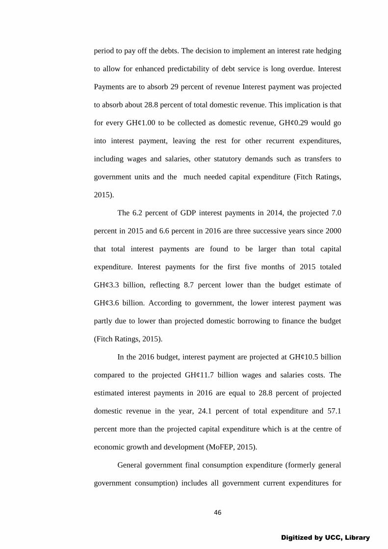
46

period to pay off the debts. The decision to implement an interest rate hedging

to allow for enhanced predictability of debt service is long overdue. Interest

Payments are to absorb 29 percent of revenue Interest payment was projected

to absorb about 28.8 percent of total domestic revenue. This implication is that

for every GH¢1.00 to be collected as domestic revenue, GH¢0.29 would go

into interest payment, leaving the rest for other recurrent expenditures,

including wages and salaries, other statutory demands such as transfers to

government units and the much needed capital expenditure (Fitch Ratings,

2015).

The 6.2 percent of GDP interest payments in 2014, the projected 7.0

percent in 2015 and 6.6 percent in 2016 are three successive years since 2000

that total interest payments are found to be larger than total capital

expenditure. Interest payments for the first five months of 2015 totaled

GH¢3.3 billion, reflecting 8.7 percent lower than the budget estimate of

GH¢3.6 billion. According to government, the lower interest payment was

partly due to lower than projected domestic borrowing to finance the budget

(Fitch Ratings, 2015).

In the 2016 budget, interest payment are projected at GH¢10.5 billion

compared to the projected GH¢11.7 billion wages and salaries costs. The

estimated interest payments in 2016 are equal to 28.8 percent of projected

domestic revenue in the year, 24.1 percent of total expenditure and 57.1

percent more than the projected capital expenditure which is at the centre of

economic growth and development (MoFEP, 2015).

General government final consumption expenditure (formerly general

government consumption) includes all government current expenditures for


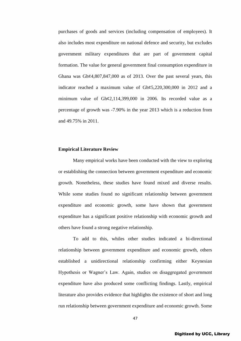
47

purchases of goods and services (including compensation of employees). It

also includes most expenditure on national defence and security, but excludes

government military expenditures that are part of government capital

formation. The value for general government final consumption expenditure in

Ghana was Gh¢4,807,847,000 as of 2013. Over the past several years, this

indicator reached a maximum value of Gh¢5,220,300,000 in 2012 and a

minimum value of Gh¢2,114,399,000 in 2006. Its recorded value as a

percentage of growth was -7.90% in the year 2013 which is a reduction from

and 49.75% in 2011.

Empirical Literature Review

Many empirical works have been conducted with the view to exploring

or establishing the connection between government expenditure and economic

growth. Nonetheless, these studies have found mixed and diverse results.

While some studies found no significant relationship between government

expenditure and economic growth, some have shown that government

expenditure has a significant positive relationship with economic growth and

others have found a strong negative relationship.

To add to this, whiles other studies indicated a bi-directional

relationship between government expenditure and economic growth, others

established a unidirectional relationship confirming either Keynesian

Hypothesis or Wagner’s Law. Again, studies on disaggregated government

expenditure have also produced some conflicting findings. Lastly, empirical

literature also provides evidence that highlights the existence of short and long

run relationship between government expenditure and economic growth. Some


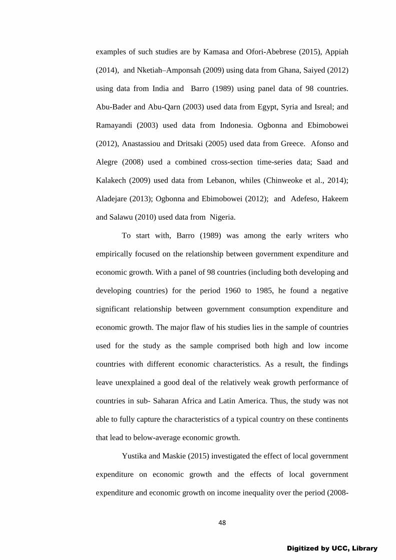
48

examples of such studies are by Kamasa and Ofori-Abebrese (2015), Appiah

(2014), and Nketiah–Amponsah (2009) using data from Ghana, Saiyed (2012)

using data from India and Barro (1989) using panel data of 98 countries.

Abu-Bader and Abu-Qarn (2003) used data from Egypt, Syria and Isreal; and

Ramayandi (2003) used data from Indonesia. Ogbonna and Ebimobowei

(2012), Anastassiou and Dritsaki (2005) used data from Greece. Afonso and

Alegre (2008) used a combined cross-section time-series data; Saad and

Kalakech (2009) used data from Lebanon, whiles (Chinweoke et al., 2014);

Aladejare (2013); Ogbonna and Ebimobowei (2012); and Adefeso, Hakeem

and Salawu (2010) used data from Nigeria.

To start with, Barro (1989) was among the early writers who

empirically focused on the relationship between government expenditure and

economic growth. With a panel of 98 countries (including both developing and

developing countries) for the period 1960 to 1985, he found a negative

significant relationship between government consumption expenditure and

economic growth. The major flaw of his studies lies in the sample of countries

used for the study as the sample comprised both high and low income

countries with different economic characteristics. As a result, the findings

leave unexplained a good deal of the relatively weak growth performance of

countries in sub- Saharan Africa and Latin America. Thus, the study was not

able to fully capture the characteristics of a typical country on these continents

that lead to below-average economic growth.

Yustika and Maskie (2015) investigated the effect of local government

expenditure on economic growth and the effects of local government

expenditure and economic growth on income inequality over the period (2008-


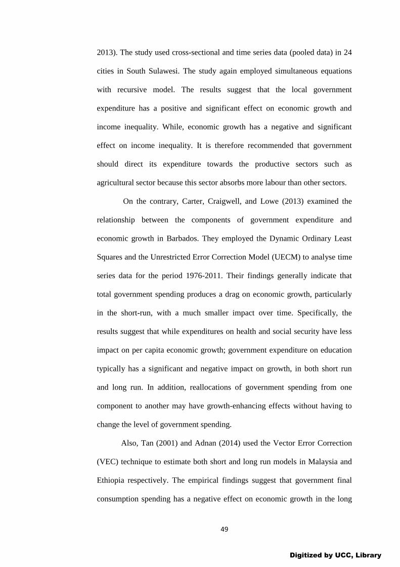
49

2013). The study used cross-sectional and time series data (pooled data) in 24

cities in South Sulawesi. The study again employed simultaneous equations

with recursive model. The results suggest that the local government

expenditure has a positive and significant effect on economic growth and

income inequality. While, economic growth has a negative and significant

effect on income inequality. It is therefore recommended that government

should direct its expenditure towards the productive sectors such as

agricultural sector because this sector absorbs more labour than other sectors.

On the contrary, Carter, Craigwell, and Lowe (2013) examined the

relationship between the components of government expenditure and

economic growth in Barbados. They employed the Dynamic Ordinary Least

Squares and the Unrestricted Error Correction Model (UECM) to analyse time

series data for the period 1976-2011. Their findings generally indicate that

total government spending produces a drag on economic growth, particularly

in the short-run, with a much smaller impact over time. Specifically, the

results suggest that while expenditures on health and social security have less

impact on per capita economic growth; government expenditure on education

typically has a significant and negative impact on growth, in both short run

and long run. In addition, reallocations of government spending from one

component to another may have growth-enhancing effects without having to

change the level of government spending.

Also, Tan (2001) and Adnan (2014) used the Vector Error Correction

(VEC) technique to estimate both short and long run models in Malaysia and

Ethiopia respectively. The empirical findings suggest that government final

consumption spending has a negative effect on economic growth in the long


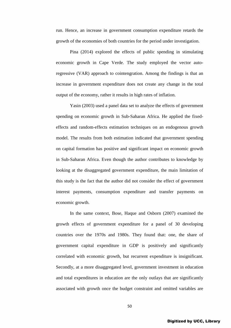
50

run. Hence, an increase in government consumption expenditure retards the

growth of the economies of both countries for the period under investigation.

Pina (2014) explored the effects of public spending in stimulating

economic growth in Cape Verde. The study employed the vector auto-

regressive (VAR) approach to cointengration. Among the findings is that an

increase in government expenditure does not create any change in the total

output of the economy, rather it results in high rates of inflation.

Yasin (2003) used a panel data set to analyze the effects of government

spending on economic growth in Sub-Saharan Africa. He applied the fixed-

effects and random-effects estimation techniques on an endogenous growth

model. The results from both estimation indicated that government spending

on capital formation has positive and significant impact on economic growth

in Sub-Saharan Africa. Even though the author contributes to knowledge by

looking at the disaggregated government expenditure, the main limitation of

this study is the fact that the author did not consider the effect of government

interest payments, consumption expenditure and transfer payments on

economic growth.

In the same context, Bose, Haque and Osborn (2007) examined the

growth effects of government expenditure for a panel of 30 developing

countries over the 1970s and 1980s. They found that: one, the share of

government capital expenditure in GDP is positively and significantly

correlated with economic growth, but recurrent expenditure is insignificant.

Secondly, at a more disaggregated level, government investment in education

and total expenditures in education are the only outlays that are significantly

associated with growth once the budget constraint and omitted variables are


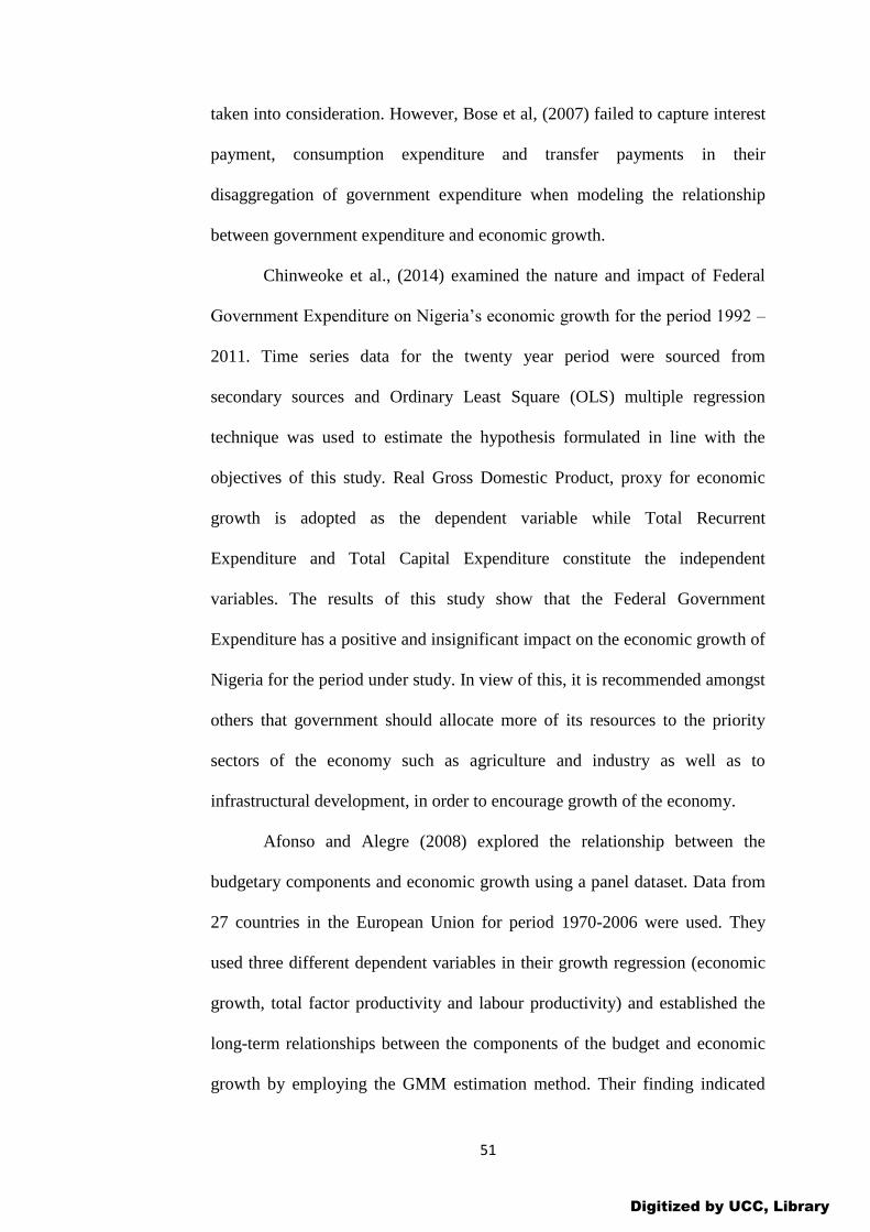
51

taken into consideration. However, Bose et al, (2007) failed to capture interest

payment, consumption expenditure and transfer payments in their

disaggregation of government expenditure when modeling the relationship

between government expenditure and economic growth.

Chinweoke et al., (2014) examined the nature and impact of Federal

Government Expenditure on Nigeria’s economic growth for the period 1992 –

2011. Time series data for the twenty year period were sourced from

secondary sources and Ordinary Least Square (OLS) multiple regression

technique was used to estimate the hypothesis formulated in line with the

objectives of this study. Real Gross Domestic Product, proxy for economic

growth is adopted as the dependent variable while Total Recurrent

Expenditure and Total Capital Expenditure constitute the independent

variables. The results of this study show that the Federal Government

Expenditure has a positive and insignificant impact on the economic growth of

Nigeria for the period under study. In view of this, it is recommended amongst

others that government should allocate more of its resources to the priority

sectors of the economy such as agriculture and industry as well as to

infrastructural development, in order to encourage growth of the economy.

Afonso and Alegre (2008) explored the relationship between the

budgetary components and economic growth using a panel dataset. Data from

27 countries in the European Union for period 1970-2006 were used. They

used three different dependent variables in their growth regression (economic

growth, total factor productivity and labour productivity) and established the

long-term relationships between the components of the budget and economic

growth by employing the GMM estimation method. Their finding indicated


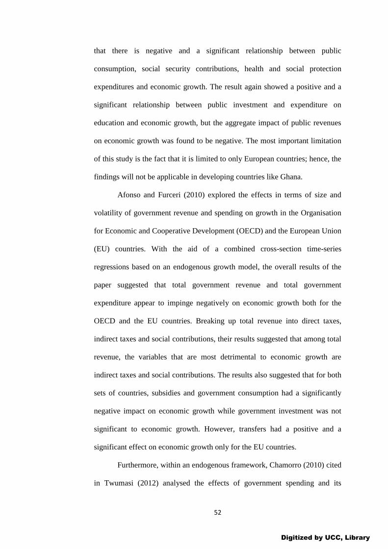
52

that there is negative and a significant relationship between public

consumption, social security contributions, health and social protection

expenditures and economic growth. The result again showed a positive and a

significant relationship between public investment and expenditure on

education and economic growth, but the aggregate impact of public revenues

on economic growth was found to be negative. The most important limitation

of this study is the fact that it is limited to only European countries; hence, the

findings will not be applicable in developing countries like Ghana.

Afonso and Furceri (2010) explored the effects in terms of size and

volatility of government revenue and spending on growth in the Organisation

for Economic and Cooperative Development (OECD) and the European Union

(EU) countries. With the aid of a combined cross-section time-series

regressions based on an endogenous growth model, the overall results of the

paper suggested that total government revenue and total government

expenditure appear to impinge negatively on economic growth both for the

OECD and the EU countries. Breaking up total revenue into direct taxes,

indirect taxes and social contributions, their results suggested that among total

revenue, the variables that are most detrimental to economic growth are

indirect taxes and social contributions. The results also suggested that for both

sets of countries, subsidies and government consumption had a significantly

negative impact on economic growth while government investment was not

significant to economic growth. However, transfers had a positive and a

significant effect on economic growth only for the EU countries.

Furthermore, within an endogenous framework, Chamorro (2010) cited

in Twumasi (2012) analysed the effects of government spending and its


53

different components on the economic growth rate in a set of low and middle-

income countries across the world over the period 1975-2000. He used the

(Arellano & Bond, 1991) GMM technique to evaluate that the growth effects

of the different expenditure components. The effects of government

expenditures on education, transport and communication were found to be

positive and that of economic affairs was negative. Spending on health and

defence however exhibited no significant relationship with economic growth.

Saad and Kalakech (2009) analysed the economic growth effects of

government expenditure in Lebanon using a disaggregated analysis based on

sectoral expenditures. In doing so, the authors employed the Vector Auto

Regression (VAR) analysis on annual data from 1962 to 2007. Using an

endogenous model, the paper found out that government spending on

education has a positive effect on economic growth in the long run and a

negative impact in the short run while the expenditure on agriculture was

shown not to affect economic growth in both time periods. On the other hand,

expenditures on both defence and health were shown to be negatively related

to economic growth only in the long run.

Using pooled time series and cross-section data for 7 countries in the

South Eastern Europe (SEE) spanning from 1995 to 2005, Alexiou (2009)

investigated the relationship between government expenditure and economic

growth. The results indicate that, government spending on capital formation

has positive and significant effect on economic growth, in contrast to

population growth which was found to be statistically insignificant.

A study was conducted to demonstrate the impact of defence

expenditure on economic growth by employing a three sector Feder-Ram


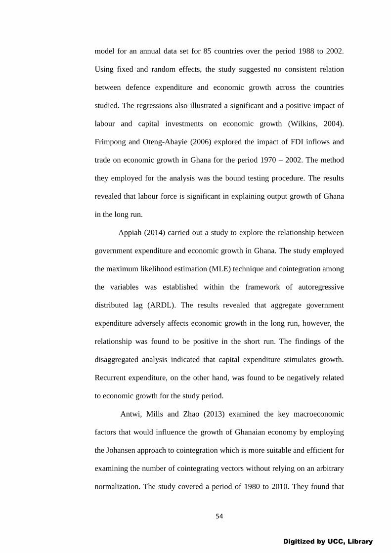
54

model for an annual data set for 85 countries over the period 1988 to 2002.

Using fixed and random effects, the study suggested no consistent relation

between defence expenditure and economic growth across the countries

studied. The regressions also illustrated a significant and a positive impact of

labour and capital investments on economic growth (Wilkins, 2004).

Frimpong and Oteng-Abayie (2006) explored the impact of FDI inflows and

trade on economic growth in Ghana for the period 1970 – 2002. The method

they employed for the analysis was the bound testing procedure. The results

revealed that labour force is significant in explaining output growth of Ghana

in the long run.

Appiah (2014) carried out a study to explore the relationship between

government expenditure and economic growth in Ghana. The study employed

the maximum likelihood estimation (MLE) technique and cointegration among

the variables was established within the framework of autoregressive

distributed lag (ARDL). The results revealed that aggregate government

expenditure adversely affects economic growth in the long run, however, the

relationship was found to be positive in the short run. The findings of the

disaggregated analysis indicated that capital expenditure stimulates growth.

Recurrent expenditure, on the other hand, was found to be negatively related

to economic growth for the study period.

Antwi, Mills and Zhao (2013) examined the key macroeconomic

factors that would influence the growth of Ghanaian economy by employing

the Johansen approach to cointegration which is more suitable and efficient for

examining the number of cointegrating vectors without relying on an arbitrary

normalization. The study covered a period of 1980 to 2010. They found that


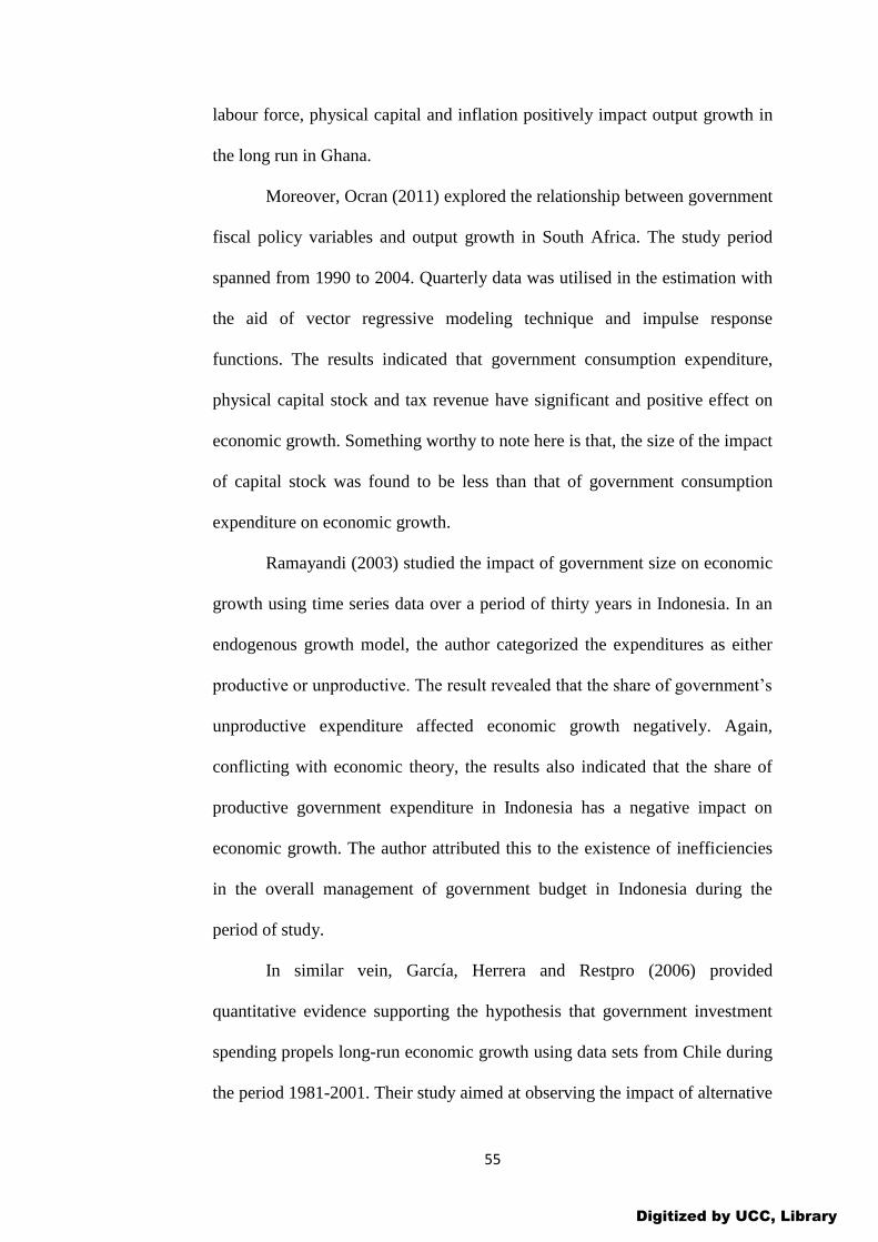
55

labour force, physical capital and inflation positively impact output growth in

the long run in Ghana.

Moreover, Ocran (2011) explored the relationship between government

fiscal policy variables and output growth in South Africa. The study period

spanned from 1990 to 2004. Quarterly data was utilised in the estimation with

the aid of vector regressive modeling technique and impulse response

functions. The results indicated that government consumption expenditure,

physical capital stock and tax revenue have significant and positive effect on

economic growth. Something worthy to note here is that, the size of the impact

of capital stock was found to be less than that of government consumption

expenditure on economic growth.

Ramayandi (2003) studied the impact of government size on economic

growth using time series data over a period of thirty years in Indonesia. In an

endogenous growth model, the author categorized the expenditures as either

productive or unproductive. The result revealed that the share of government’s

unproductive expenditure affected economic growth negatively. Again,

conflicting with economic theory, the results also indicated that the share of

productive government expenditure in Indonesia has a negative impact on

economic growth. The author attributed this to the existence of inefficiencies

in the overall management of government budget in Indonesia during the

period of study.

In similar vein, García, Herrera and Restpro (2006) provided

quantitative evidence supporting the hypothesis that government investment

spending propels long-run economic growth using data sets from Chile during

the period 1981-2001. Their study aimed at observing the impact of alternative


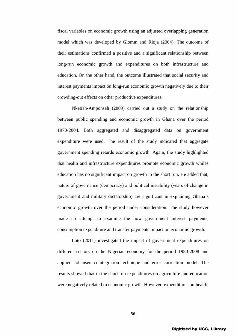
56

fiscal variables on economic growth using an adjusted overlapping generation

model which was developed by Glomm and Rioja (2004). The outcome of

their estimations confirmed a positive and a significant relationship between

long-run economic growth and expenditures on both infrastructure and

education. On the other hand, the outcome illustrated that social security and

interest payments impact on long-run economic growth negatively due to their

crowding-out effects on other productive expenditures.

Nketiah-Amponsah (2009) carried out a study on the relationship

between public spending and economic growth in Ghana over the period

1970-2004. Both aggregated and disaggregated data on government

expenditure were used. The result of the study indicated that aggregate

government spending retards economic growth. Again, the study highlighted

that health and infrastructure expenditures promote economic growth whiles

education has no significant impact on growth in the short run. He added that,

nature of governance (democracy) and political instability (years of change in

government and military dictatorship) are significant in explaining Ghana’s

economic growth over the period under consideration. The study however

made no attempt to examine the how government interest payments,

consumption expenditure and transfer payments impact on economic growth.

Loto (2011) investigated the impact of government expenditures on

different sectors on the Nigerian economy for the period 1980-2008 and

applied Johansen cointegration technique and error correction model. The

results showed that in the short run expenditures on agriculture and education

were negatively related to economic growth. However, expenditures on health,


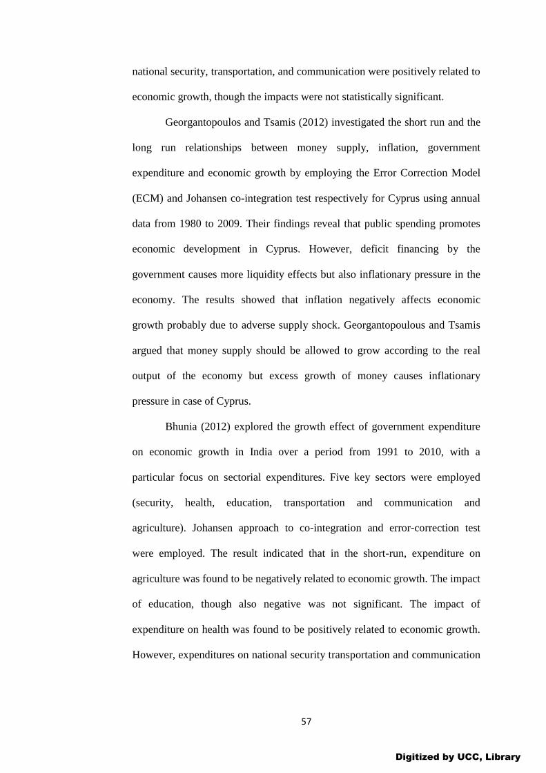
57

national security, transportation, and communication were positively related to

economic growth, though the impacts were not statistically significant.

Georgantopoulos and Tsamis (2012) investigated the short run and the

long run relationships between money supply, inflation, government

expenditure and economic growth by employing the Error Correction Model

(ECM) and Johansen co-integration test respectively for Cyprus using annual

data from 1980 to 2009. Their findings reveal that public spending promotes

economic development in Cyprus. However, deficit financing by the

government causes more liquidity effects but also inflationary pressure in the

economy. The results showed that inflation negatively affects economic

growth probably due to adverse supply shock. Georgantopoulous and Tsamis

argued that money supply should be allowed to grow according to the real

output of the economy but excess growth of money causes inflationary

pressure in case of Cyprus.

Bhunia (2012) explored the growth effect of government expenditure

on economic growth in India over a period from 1991 to 2010, with a

particular focus on sectorial expenditures. Five key sectors were employed

(security, health, education, transportation and communication and

agriculture). Johansen approach to co-integration and error-correction test

were employed. The result indicated that in the short-run, expenditure on

agriculture was found to be negatively related to economic growth. The impact

of education, though also negative was not significant. The impact of

expenditure on health was found to be positively related to economic growth.

However, expenditures on national security transportation and communication


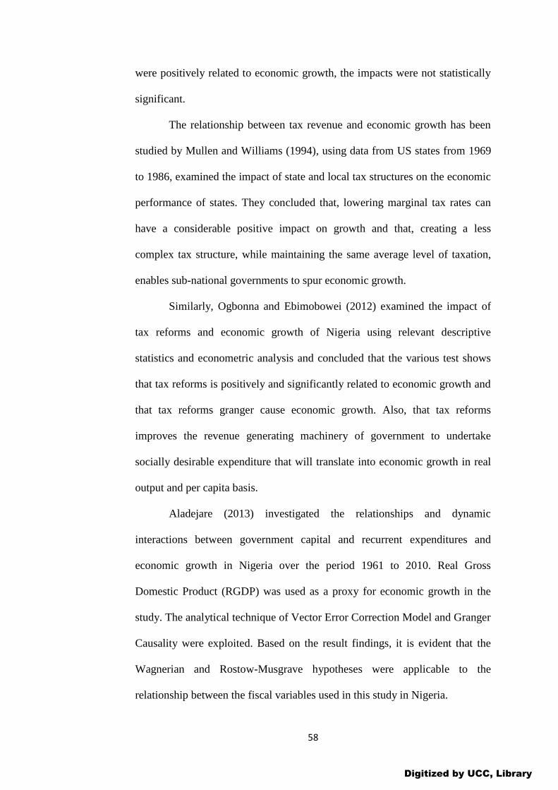
58

were positively related to economic growth, the impacts were not statistically

significant.

The relationship between tax revenue and economic growth has been

studied by Mullen and Williams (1994), using data from US states from 1969

to 1986, examined the impact of state and local tax structures on the economic

performance of states. They concluded that, lowering marginal tax rates can

have a considerable positive impact on growth and that, creating a less

complex tax structure, while maintaining the same average level of taxation,

enables sub-national governments to spur economic growth.

Similarly, Ogbonna and Ebimobowei (2012) examined the impact of

tax reforms and economic growth of Nigeria using relevant descriptive

statistics and econometric analysis and concluded that the various test shows

that tax reforms is positively and significantly related to economic growth and

that tax reforms granger cause economic growth. Also, that tax reforms

improves the revenue generating machinery of government to undertake

socially desirable expenditure that will translate into economic growth in real

output and per capita basis.

Aladejare (2013) investigated the relationships and dynamic

interactions between government capital and recurrent expenditures and

economic growth in Nigeria over the period 1961 to 2010. Real Gross

Domestic Product (RGDP) was used as a proxy for economic growth in the

study. The analytical technique of Vector Error Correction Model and Granger

Causality were exploited. Based on the result findings, it is evident that the

Wagnerian and Rostow-Musgrave hypotheses were applicable to the

relationship between the fiscal variables used in this study in Nigeria.


59

Okoro (2013) investigated the impact of government spending on the

Nigerian economic growth using time series data for the period 1980 to 2011.

The ordinary least square multiple regression analysis was employed to

estimate the model specified. Real Gross Domestic Product (RGDP) was

adopted as the dependent variable while government capital expenditure and

government recurrent expenditure represents the independent variables. With

the application of Granger Causality test, Johansen Cointegration Test and

Error Correction Model, the result shows that there exists a long-run

equilibrium relationship between government spending and economic growth

in Nigeria. The short-run dynamics adjusts to the long-run equilibrium at the

rate of 60% per annum.

Ogundipe and Oluwatobi (2013) examined the impact of both

government recurrent and capital expenditure on growth performance using an

econometric analysis based on Johansen technique for the period of 1970-

2009. The study found the component of total expenditure impacting

negatively (except education and health) and insignificantly on growth rate;

further diagnosis test reveals capital expenditure may likely induce significant

impact on growth rate in the long-run. Notable recommendations include,

proper management of capital and recurrent expenditure, proper surveillance

and quantification of capital spending in order to boost social and human

capital, and development of sound institutions void of political influences.

Chude and Chude (2013) investigated the effects of public expenditure

on education on economic growth in Nigeria over a period from 1977 to 2012,

with particular focus on disaggregated and sectoral expenditures analysis. The

study used ex-post facto research design and applied time series econometrics


60

technique to examine the long and short run effects of public expenditure on

economic growth in Nigeria. The results indicated that total expenditure on

education is highly and statistically significant and have positive relationship

on economic growth in Nigeria in the long run. The result has an important

implication in terms of policy and budget implementation in Nigeria. They

concluded that economic growth is clearly impacted by factors both

exogenous and endogenous to the public expenditure in Nigeria.

Hence, the study recommended that there is need for government to

reduce its budgetary allocation to recurrent expenditure on education and place

more emphasis on the capital expenditures so as to accelerate economic

growth of Nigeria and that Government should direct its expenditure towards

the productive sectors like education as it would reduce the cost of doing

business as well as raise the standard living of poor ones in the country.

Musaba, Chilonda and Matchaya (2013) examined the impact of

government sectorial expenditure on economic growth in Malawi by using

time series data from 1980 to 2007. Cointegration analysis in the context of

an error correction model was employed to estimate the growth effects of

government expenditures on agriculture, education, health, defence, social

protection and transport and communication. The short run results showed no

significant relationship between government sectorial expenditure and

economic growth. The long run results showed a significant positive effect of

expenditures on agriculture and defence on economic growth. The

expenditures on education, health, social protection and transportation and

communication were negatively related to economic growth. To boost


61

economic growth efficient management of resources allocated to all sectors

should be emphasized.

On the direction of causality between government expenditure growth

and economic growth, Kamasa and Ofori-Abebrese (2015) empirically

analysed the causal relationship between government expenditure growth and

GDP growth in Ghana for the period 1980–2010. They employed vector

autoregressive (VAR)/Granger causality analysis developed by Sims (1980)

and Granger (1969). Granger causality test conducted provided a

unidirectional causality running from GDP growth to government expenditure

growth. This finding provides support for the Wagner’s law of expanding state

activities for Ghana. The result also suggests that government must focus on

policies that would create the enabling environment for growth to thrive rather

than increasing its expenditure with the aim of increasing GDP growth.

However, the study did not make clear which specific polices could be

adopted to create the needed enabling environment for economic growth to

occur.

Again, Al-Faris (2002) explored the relationship between government

expenditure and economic growth in the Gulf Cooperation Council (GCC)

countries: Saudi Arabia, the United Arab Emirates, Kuwait, Oman, Bahrain

and Qatar using time series annual data from 1970-1997. Multivariate

cointegration approach was used. The results revealed a unidirectional

causality between government expenditure and economic growth with the

causality running from GDP growth to public expenditure, which supports

Wagner’s law as in the case of Kamasa and Ofori-Abebrese (2015) and

Appiah (2014) for Ghana. It must be emphasized at this point that, though


62

these findings provide support for the Wagner’s law, conclusions drawn from

the Al-Faris (2002) cannot be applied to Ghana. The reason is that the

countries involved in his study are a set of countries experienced in oil

exploration hence government expenditure and its components may be totally

different from what pertains to Ghana.

Kunofiwa and Odhiambo (2013) investigated the dynamic causal

relationship between government expenditure and economic growth using data

from Zimbabwe. The study employed the newly proposed ARDL-bounds

testing approach to examine this linkage. In order to address the omission of

variable bias, the study incorporated unemployment as an intermittent variable

between economic growth and government spending–thereby creating a

simple multivariate model. The empirical findings of this study showed that,

although both government expenditure and economic growth Granger-cases

each other in the short run, in the long run, it is economic growth that

Granger-causes government expenditure. Other results indicated that there is a

short-run unidirectional causality from both economic growth and government

expenditure to unemployment. The study did not try to consider any form of

government expenditure disaggregation and economic growth relationship.

Furthermore, Rehman, Iqbal and Siddiqi (2010) examined the nature

and direction of causality in Pakistan between public expenditure and national

income along with various selected components of public expenditure by

applying Toda-Yamamoto causality test to Pakistan for the period of 1971 to

2006. The study finds a unidirectional causality running from GDP to

government expenditure, which supports the Wagner’s law.


63

However, Ebaidalla (2013) investigated the nature and direction of

causality between government expenditure and national income in Sudan

using Granger causality test and Error Correction Model (ECM) for the period

1970-2008. The result of cointegration test suggested a long-run relationship

between government expenditure and national income in Sudan. The causality

test indicated a unidirectional causality running from government expenditure

to national income, both in the short and long-run. Thus, the results support

the Keynesian proposition, which states that public spending is an important

exogenous factor for stimulating national income. Moreover, the study

concludes that fiscal policy in Sudan plays a vital role in stabilizing the

economy and achieving economic goals.

To add to this, Al-Fawwaz and Al-Sawai’e (2013) examined the

relationship between real gross domestic product and government

expenditures in Jordan for the period 1990-2010 by using vector

autoregressive model (VAR). The empirical results indicated that there is a

unidirectional effect from real government expenditures to real gross domestic

product. This result does not support Wagner's law, but support the

Keynesian's hypothesis, which indicated that expenditure is a part of the

effective demand, which affects the gross domestic product.

On the same platform, Saiyed (2012) investigated the bi-directional

causal relationship between economic growth and growth of public

expenditure in India during the Post Economic Reforms period from 1992 to

2012. First, impact of economic growth on public expenditure is investigated

and then influence of public expenditure on economic growth is examined

during 1992 to 2012. Cross-sectional analysis of data from 21 years during


64

1992 to 2012 of India showed significant bi-directional causal relationship

between year-wise number of national income (GDP) and public expenditure.

Also, Abu-Bader and Abu-Qarn (2003) used data from Egypt, Israel

and Syria. They employed the multivariate cointegration and the variance

decomposition approach to examine the connection between government

expenditure, military spending and economic growth for the periods 1975-

1998 in Egypt, 1967-1998 in Israel and 1973-1998 in Syria. The result

indicated a bi-directional and a long-run negative relationship between

government spending and economic growth when variables were tested within

a bivariate framework. Also, the causality test within a trivariate system

(where government spending was broken down into share of government

civilian expenditures in GDP and military expenditure) showed that military

expenditure has a negative impact on economic growth in all the three

countries, but civilian government expenditures exhibited a positive impact on

economic growth for both Israel and Egypt.

Again, Oyinlola and Akinnibosun (2013) examined the relationship

between public expenditure and economic growth in Nigeria during the period

1970-2009. A disaggregated public expenditure level was employed using the

Gregory-Hansen structural breaks cointegration technique. The result confirms

Wagner’s law in two models in the long run; there was a break in 1993 in

which the political crisis that engulfed the nation was accountable. The result

also shows that economic growth and development are the main objectives of

government expenditure, especially investment in infrastructure and human

resources all of which falls under social and community services. They


65

suggested based on the result that, there should be efforts to maintain adequate

levels of investment in social and economic infrastructure.

Summary of the Literature Review

This chapter reviewed comprehensively the theoretical and empirical

literature relevant to the study. The theoretical review covered the following

areas: theoretical background of government expenditure and economic

growth nexus; theories of growth with specific emphasis on the neoclassical

(Solow-Swan, Peacock-Shaw) growth models and endogenous growth model

including Afonso-Alegre growth theory; the role of the government in

economic growth; and some theories of government expenditure growth.

Whiles the empirical review considered empirical works on the government

expenditure growth and economic growth relationship.

The review revealed that, government played a crucial role in

enhancing the growth of the economy through its spending policies. However,

if the government size becomes excessively large the pace of economic

growth will slow down.

The review found no theoretical justification for disaggregating

government expenditure. However, a lot of empirical studies have indicated

that different government expenditure components have different impact on

the growth of an economy. Therefore, studying the relationship between

government expenditure components and economic growth in Ghana is

deemed appropriate so that policy makers will be informed as to which

government expenditure components should be given much consideration if

the focus is to achieve economic growth.


66

Lastly, many empirical studies have basically laid emphasis on either

aggregated or disaggregated data on government expenditure and found mixed

and dissimilar findings on the relationship between government expenditure

and economic growth. This study will therefore focus on relationship between

government interest payments, transfer payments and consumption

expenditure, and economic growth in Ghana.


67

CHAPTER THREE

METHODOLOGY

Introduction

This chapter highlights the methodological framework suitable for

carrying out this research with explicit emphasis on the research design, model

specification, justification and measurement of the variables, nature and

source of data, estimation techniques and, post estimation tests.

Research Design

Considering the objectives of the study, the positivist philosophy was

deemed suitable and was employed for the study. The reason for the adoption

of this paradigm is that, the positivists maintain that the reality is stable and

can be observed and described from an impartial standpoint without

interfering with the phenomena under investigation (Levin, 1988). It makes it

possible for the researcher to examine social processes in a more objective

manner so as to describe relationships between variables being investigated.

Again, this paradigm allows the use of quantitative approach to research which

makes it appropriate for the development of mathematical models in order to

explore the relationship between quantitative measurements.

On the basis of the positivist philosophy, the quantitative approach is

considered appropriate and was accordingly adopted for the study. Moreover,

the quantitative approach allows the investigator to put the social world into a

structure of causality and dissolves the role of human effect through the use of

a quantitative instrument such as multivariate statistical analysis in analysing

data as used in this study. More importantly, because what the study seeks to


68

achieve is explanatory in nature, it adopted the explanatory research under the

quantitative approach.

Theoretical Model Specification

The study adopted the neoclassical growth model which argues that

economic growth can be achieved when capital and labour are augmented by

additional factors of production in the production function.

The Solow (1956) growth model describes economic growth as

emanating from the combination of two inputs capital (K) and labour (L)

( , )t t tY f K L (1)

The critical question that emanates from equation (1) is how much of

the increase in output can be assigned solely to variations in capital and

labour. The reason is that there is a possibility of other factors, aside labour

and capital, which can influence output. Solow (1956), in order to address this

challenge, disintegrates change in output into three components namely:

physical capital accumulation, growth of labour force and growth of total

factor productivity (TFP). The growth of TFP reflects the adjustment in output

that is not explained by variation in physical inputs such as labour and capital

in the model. As a result, the TFP may be interpreted as the effect of

exogenous technological progress that can equally be observed in increasing

productive efficiency. Solow, to be able to explain this, employed the Cobb-

Douglas production function expressed as:

( , , , )t t t tY f A K L (2)


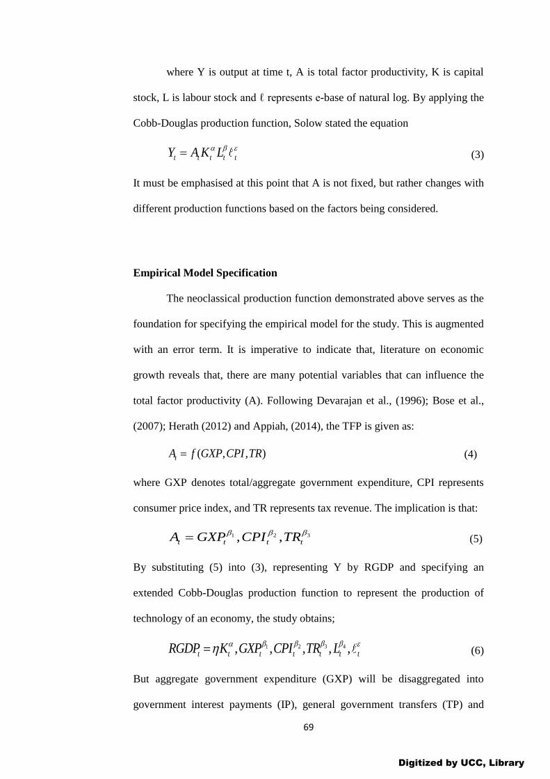
69

where Y is output at time t, A is total factor productivity, K is capital

stock, L is labour stock and ℓ represents e-base of natural log. By applying the

Cobb-Douglas production function, Solow stated the equation

t t t t tY A K L (3)

It must be emphasised at this point that A is not fixed, but rather changes with

different production functions based on the factors being considered.

Empirical Model Specification

The neoclassical production function demonstrated above serves as the

foundation for specifying the empirical model for the study. This is augmented

with an error term. It is imperative to indicate that, literature on economic

growth reveals that, there are many potential variables that can influence the

total factor productivity (A). Following Devarajan et al., (1996); Bose et al.,

(2007); Herath (2012) and Appiah, (2014), the TFP is given as:

( , , )tA f GXP CPI TR (4)

where GXP denotes total/aggregate government expenditure, CPI represents

consumer price index, and TR represents tax revenue. The implication is that:

31 2, ,t t t tA GXP CPI TR

(5)

By substituting (5) into (3), representing Y by RGDP and specifying an

extended Cobb-Douglas production function to represent the production of

technology of an economy, the study obtains;

31 2 4, , , , ,t t t t t t tRGDP K GXP CPI TR L (6)

But aggregate government expenditure (GXP) will be disaggregated into

government interest payments (IP), general government transfers (TP) and


70

general government final consumption expenditure (CXP). Thus,

GXP IP TP CXP (7)

By substituting (7) into (6), (8) is obtained;

3 5 61 2 4, , , , , , ,t t t t t t t t tRGDP K IP TP CXP CPI TR L (8)

By taking the logarithm of the some of the variables (RGDP, IP, TP, CPI and

K) in equation (8), (9) is obtained. The other variables such as CXP, TR and

L are not logged because they are measured in percentages.

1 2 3

4 5 6

ln ln ln ln

ln ln

t t t t

t t t t t

GDP K IP TP CXP

CPI TR L

(9)

Letting 0ln and ln 1t , equation (9) can be written as

0 1 2 3

4 5 6

ln ln ln ln

ln

t t t t t

t t t t

RGDP K IP TP CXP

CPI TR L

(10)

To be able to estimate the growth of the economy, we difference equation (10)

to obtain,

1 0 1 1 1 2 1

3 1 4 1 5 1

6 1

ln ln (ln ln ) (ln ln ) (ln ln )

( ) (ln ln ) ( )

( )

t t t t t t t t

t t t t t t

t t t

RGDP RGDP K K IP IP TP TP

CXP CXP CPI CPI TR TR

L L

(11)

Equation (11) above can be re-written as

0 1 2 3

4 5 6

ln ln ln ln

ln

t t t t t

t t t t

RGDP K IP TP CXP

CPI TR L

(12)


71

Definition and Measurement of Variables

Economic growth can be explained as the continuous or sustained

increase in the real gross domestic product (GDP) or national product of an

economy overtime. Nonetheless, this study uses real GDP (RGDP) to proxy

for economic growth. The reason behind this is that other researchers

(Aladejare, 2013; Okoro, 2013; Al-Fawwaz & Al-Sawai’e, 2013; Chinweoke

et al, 2014) have used it in their work as dependent variable. Real GDP is the

nominal GDP adjusted for inflation.

Gross fixed capital formation is used to proxy capital stock (K). Gross

fixed capital formation is defined as the total value of additions to fixed assets

by domestic enterprises, less disposals of fixed assets during the year, plus

additions to the value of non-produced assets such as discoveries of mineral

deposits, plants, machinery and equipment purchases; and the construction of

infrastructure and commercial and industrial buildings (Baafi, 2010; Barro,

1996). Gross fixed capital formation has generally been considered as the

engine of growth of the Ghanaian economy as in most other economies due

the additions it makes to capital stock. It is an important factor in the

determination of aggregate output. All other things being equal, an increase in

the level of capital formation will improve the economy’s productivity

potential and therefore economic growth. It contributes to economic growth

not only through the additions it makes to the stock of capital but also it offers

many potential advantages as both a source of financial capital and a source of

skills and technology transfer (Amoako-Gyampah & Acquaah, 2008). The size

of physical capital stock positively affects the level of aggregate demand and

also determines the productive capacity of the economy. It is important to


72

emphasize that high rate of capital formation (investment) results in high

economic growth (Barro, Mankiw & Sala-i-Martin, 1992). Therefore, the

coefficient of physical capital stock is expected to be positive.

Government interest payments (IP) refer to interest payments on

government debt. This consists of interest payments on long-term bonds, long-

term loans, and other debt instruments to domestic and foreign residents.

Government payments on long-term debt are actually the amounts of interest

paid by the borrower in foreign currency, goods, or services in the year

specified. Oyinlola and Akinnibosun (2013) argue that total debt outstanding

(domestic plus external debt) is inversely related to economic growth. But

total debt comprises the principal borrowed and its associated interest. It is

known that, loans themselves are not detrimental to growth if properly put to

use. Hence, it is expected that the estimate of growth is negative for

government interest payments (Garcia, Herrera & Restpro, 2006).

Government transfer payments (TP) are the expenditures made by

government that do not represent purchases of goods or services but simply

transfer of income from taxpayers to program recipients (DeLong, 2002, cited

in Twumasi, 2012). Transfer payments unlike government purchases of goods

and services represent government outlays for which no direct products or

services are obtained. Transfers consist of the issuance of income to the

private sector and they include social security, gratuities and pension

payments. It is therefore an important component of household income,

especially for the poor, and plays an important role in reducing poverty. It is

thus, expected to result in direct increases in households’ disposable income.

Hence, high levels of spending on transfers are expected to lead to increases in


73

households’ disposable income and therefore consumption, which will in turn

positively affect aggregate demand and economic growth.

Again, general government final consumption expenditure (CXP) -

formerly general government consumption - includes all government current

expenditures for purchases of goods and services (including compensation of

employees) as percentage of GDP. It also includes most expenditures on

national defense and security, but excludes government military expenditures

that are part of government capital formation. Barro (1990) regarded

government consumption payments as that part of government expenditures

that enter into the household utility functions. As a result, Barro argues that

such expenditures do not affect production opportunities and consequently do

not affect the social rate of return on investment. Increases in such

expenditures must be accompanied by a proportional increase in taxes or

borrowing or some amount of both to finance the increased expenditures. If

however the government finances the additional expenses through borrowing,

then it can have a crowding-out effect on private investments which may cause

output to fall accordingly. This is because government borrowing may draw

resources from the private sector and also may drive up interest rates which

can also adversely affect private investments.

On the other hand, if the government decides to finance these expenses

with taxes, then an increase in government’s recurrent expenditures will bring

about rises in taxes which will cause households consumption to fall.

According to Barro and Sala-i-Martin (1992), it will also lower private rate of

return on investments. This follows that an increase in government recurrent

expenditures lowers the economy's steady-state growth rate (Barro & Sala-I-


74

Martin, 1992). Therefore, the impact of government consumption spending on

economic growth is expected to be negative.

Consumer Price Index (CPI) is a measure that captures the changes in

the price level of a market basket of consumer goods and services purchased

by the household. In this study, the CPI is employed to control for the effect of

high oil price on domestic goods and services. Rapid increases in the general

price level of the economy may result in uncertainty about the future

profitability of investment projects. This is because, higher prices of consumer

goods and services may dampen demand for goods and services in the

economy and for this reason, investors may resort to more conservative

investment strategies than would otherwise be the case, eventually leading to

lower levels of investment and economic growth. As a result, the coefficient of

CPI is expected to be negative (Georgantopoulos & Tsamis, 2012).

Tax revenue (TR) refers to compulsory transfers from individuals,

firms and organizations to the central government for public purposes. Certain

compulsory transfers such as fines, penalties and most social security

contributions are excluded. Refunds and corrections of erroneously collected

tax revenue are treated as negative revenue. It is measured as tax revenue as a

percentage of GDP. Taxes are mandatory payments, ruled by laws. Tax

revenue is collected from the whole society with differentiated intensity,

inspired by considerations of justice, efficiency and effectiveness. The total

tax revenue is the sum of the revenues of different kind of taxes, depending on

what is taxed. These may include revenue of personal and company income

(direct taxes); wealth and assets as real estates and houses; the domestic

economic transactions (indirect taxes); international trade, typically through


75

import duties; custom duties; revenue from export. The coefficient of tax

revenue is expected to be positive.

Labour force (L) consists of the proportion of the population that is

economically active. In this study, it comprises persons aged 15 years to 64

years, who could potentially be economically active, as a percentage of the

total population. A major source of economic growth in the modern economy

has been the size of labour force in the economy. Jayaraman and Singh (2007)

maintained that, there cannot be growth without the involvement of labour.

Solow (1956) and Swan (1956) asserted that labour force should be

incorporated in the growth model because of its impact on the work force,

hence the inclusion of labour force in the study. All things being equal, the

higher the labour force the higher the supply of labour and hence output. It is

therefore expected that an increase in labour force will lead to an increase in

total employment and its coefficient is expected to be positive.

However, the positive relationship will be achieved depending on the

ability of the economic system to absorb and productively employ these added

workers, an ability largely associated with the rate and type of capital

accumulation and the availability of related factors such as managerial and

administrative skills (Amoako-Gyampah & Acquaah, 2008)

Nature and Sources of Data

A quarterly time series data for Ghana from 1984 to 2015 were used

for the study. The original data were obtained in an annual. The data on real

GDP, government consumption expenditure, government interest payment,

gross fixed capital formation, tax revenue, consumer price index and labour


76

force were obtained from the World Bank (2014), but data on government

general transfers was sourced from the Ministry of Finance and Economic

Planning Fiscal Data (MoFEP, 2014). Extrapolation was used to expand the

original datasets from 2013 to 2015. The quarterly data were generated from

the annual datasets through interpolation using Gandolfo (1981) algorithm.

Estimation Technique

The study utilized the Maximum Likelihood Estimation (MLE)

technique to examine the relationship between government expenditure

components and economic growth. The MLE technique is a statistical method

for estimating population parameters (such as the mean and variance) from

sample data, which selects as estimates, those parameter values maximizing

the probability of obtaining the observed data. The major advantages

associated with this estimation technique are that: the MLE procedure can be

applied to a number of models and it commonly generates estimators with

excellent asymptotic properties (Davidson & MacKinnon, 2004). Moreover,

several statistical software packages provide excellent algorithms for

maximum likelihood estimates and for many commonly used distributions.

This helps to alleviate the computational complexity of the MLE.

To examine the direction of causality between government expenditure

and economic growth, the study used the Granger causality test within the

framework of cointegration and error-correction models. The testing

procedure for this involves a number of steps which include:


77

One, the study explored the time series properties of the data by

employing the Augmented Dickey-Fuller (ADF) and the Phillip-Perron (PP)

test to check for the order of integration.

Two, the study proceeds to investigate the short-run and long run

relationships between the variables using the maximum likelihood based

approach - Autoregressive Distributed Lag (ARDL) approach to cointegration

proposed by Pesaran and Shin (1998). The ARDL approach to cointegration is

argued to be the single equation equivalence of the maximum likelihood

approach of Phillips and Hansen (1990) fully modified ordinary least squares

procedure (Pesaran & Shin, 1998).

Three, the stability and diagnostic test statistics of the ARDL model is

observed to ensure the reliability and the goodness of fit of the model. Fourth

and last, the study applied Granger-causality to test for the causality between

government expenditure and economic growth. The causality test is preceded

by cointegration testing since the presence of cointegrated relationships has

implications for the way in which causality testing is carried out.

Unit Root Tests

In order to avoid the generation of spurious regression normally

associated with time series data, the growth model specified above requires the

test for the existence of unit root for each of the variables. Thus, it is crucial to

test for the statistical properties of variables when dealing with time series

data. The reason is that time series data are seldom stationary at level forms. A

time series is said to be stationary if its mean, variance and autocovariances

are independent of time. Generally, regression associated with non-stationary


78

time series produces spurious results or regression. This is the situation when

the regression results show a high and significant relationship among variables

when no relationship actually exist. Again, with spurious results, the usual test

statistics (t, F, DW, and R2) will not have standard distributions if some of the

variables in the model have unit roots (Stock & Watson, 1988).

A wide range of unit root tests can be used to determine the stationarity

of the series. The purpose of the test is to ensure generation of a reliable result

due to the inherent individual weaknesses of the various techniques. Against

this background, the study employed both the Phillip Perron (PP) and the

Augmented Dickey-Fuller (ADF) tests.

Even though these tests have common features, they differ regarding

the way they correct for autocorrelation in the residuals. The PP non-

parametric test generalises the ADF procedure, by allowing for less restrictive

assumptions for the time series being studied.

The lag-length is chosen using the Akaike Information Criteria (AIC)

and Swartz Bayesian Criterion (SBC) for both the ADF and PP test. The

sensitivity of ADF tests to lag selection makes the PP test an important

additional tool for making inferences about unit roots. The basic formulation

of the ADF is:

1 1

1

p

t t i t t

i

X t X X

(13)

Where Xt represents the series at time t, Δ is the first difference

operator, α, δ, , and λ are parameters to be estimated and ε is the stochastic

random disturbance term. Accordingly, the ADF and the PP test the null


79

hypothesis that a series contains unit root (non-stationary) against the

alternative hypothesis of no unit root (stationary). That is:

0 : 0H

1 : 0H

If the tau value or t-statistic is more negative than the critical values, the null

hypothesis is rejected and we conclude that the series is stationary. On the

contrary, if the tau statistic is less negative than the critical values, the null

hypothesis is accepted and the conclusion is that the series is non-stationary.

Cointegration Test

Quite a number of techniques exist for testing the existence of

equilibrium long-run relationship among time series variables. Most time

series studies have employed the Engle and Granger (1987), the Fully

Modified Ordinary Least Squares (FMOLS) procedures of Phillips and

Hansen (1990); the Johansen (1988); or the Johansen and Juselius (1990); and

the Autoregressive Distributed Lag (ARDL) approach by Pesaran and Shin

(1998); and Pesaran et al., (2001) to establish the long-run relationship in

bivariate and multivariate frameworks.

The study adopted the currently developed Bounds Test approach to

cointegration by Pesaran and Pesaran (1997), Pesaran and Shin (1998) which

was further expanded by Pesaran et al. (2001). The bounds test approach to

cointegration is adopted for this study due to its advantages over the Johansen

approach to cointegration.


80

To begin with, the bounds test approach to cointegration produces

more robust results in small samples than the Johansen approach. Thus, ARDL

technique is more suitable and efficient for small and finite samples compared

with the Johansen approach that requires large data samples for one to get a

valid result (Pesaran & Shin, 1998).

Also, the ARDL approach to cointegration is most appropriate

compared to the other cointegration procedures in the sense that, the other

approaches to cointegration require that all regressors be integrated of the

same other, but the ARDL approach can be used whether the regressors are

integrated of order one or order zero (.i.e. I(1) or I(0) variables). This implies

that the ARDL technique rules out the pre-testing problems related to standard

cointegration, which requires that the variables be classified into I (0) or I (1)

(Pesaran, Shin, & Smith, 2001). For example, if we are not certain about the

stationarity properties of the data, then using the ARDL technique is the most

appropriate model for empirical work.

The first and foremost step in any cointegration procedure is to identify

the degree of integration of each variable in the model. Nevertheless, this

depends on which unit roots test one employs and different unit root tests

could lead to contradictory results (Bahmani-Oskooee, 2002). Employing

conventional unit roots tests such as the Augmented Dickey Fuller and the

Phillips-Perron tests for instance, may lead to an erroneous conclusion that

unit root is present in a series that is actually stationary around a one-time

structural break (Perron, 1991). The ARDL approach is appropriate due to its

inherent ability to mitigate these problems.


81

One complexity associated with the Johansen cointegration technique

is that the ARDL approach to cointegration shuns what pertains to the large

number of choices that must be made. These include choices such as the

number of endogenous and exogenous variables to be included in the model,

the treatment of deterministic elements, as well as the order of VAR and the

optimal number of lags to be used. The estimation procedures are quite

responsive to the method used to make these choices and decisions (Pesaran &

Shin, 1999).

Finally, with the ARDL technique, it is possible that different variables

have different optimal lags lengths, whereas in Johansen-type models this is

not allowed.

Pesaran and Pesaran (1997) maintain that, the ARDL technique

comprise basic two steps. One, the existence of any long-term relationship

between the variables of interest is determined using an F-test. Two, the

analysis is to estimate the coefficients of the long-run relationship and

determine their values, followed by the estimation of the short-run elasticity of

the variables with the error correction representation of the ARDL model. By

employing the ECM version of ARDL, the speed of adjustment to equilibrium

will be determined.

The study advanced to estimate the short run and long run elasticities

by employing the Unrestricted Error Correction Model (UECM) that has

unrestricted intercepts and no trends based on the assumption made by Pesaran

et al. (2001). Based the analysis, equation (12) can be specified in ARDL

framework as:


82

0 1 2 3 4

1 1 1 1

5 6 7 8

1 1 1 1

1 1 2 1 3 1 4 1 5 1 6

ln ln ln ln ln

ln

ln ln ln ln ln

p p p p

t i t i i t i i t i i t i

i i i i

p p p p

i t i i t i i t i i t i

i i i i

t t t t t

RGDP RGDP K IP TP

CXP CPI TR L

RGDP K IP TP CXP CP

1

7 1 8 1 ..............................................................................................(14)

t

t t t

I

TR L

Where△ represents the first difference operator, P is the lag order selected by

the Schwarz Bayesian Criterion (SBC), α0 is the drift parameter, and t is the

error term which is 𝑁 (0, 𝛿2). The parameters α𝑖𝑗 are short-run parameters and

δ𝑖𝑗 are the long-run multipliers.

The examination of the relationship between government expenditure

components and economic growth commences by estimating equation (14)

with the bounds test using the OLS method, which is generally the first and

foremost procedure in the ARDL model. The F-test or Wald test is employed

for the examination of the existence of long-run relationship among the

variables in equations (13) given as follows: The null hypotheses of no long-

run relationship among the variables in equations (14) is tested against the

alternative hypotheses of a long- run relationship as follows:

0 1 2 3 4 5 6 7 8: 0H

1 1 2 3 4 5 6 7 8: 0H

The presence of cointegration among the variables under investigation is

tested based on the F-statistics or Wald statistics. Given that, the asymptotic

distribution of the F-statistic is non-standard without taking into account the

independent variables being I (0) or I (1), Pesaran and Pesaran (1997) have

provided two sets of critical values for the different numbers of regressors (k),

and whether the ARDL model contains an intercept and/or trend. As a result,


83

the calculated F-statistic is compared with these sets of critical values

developed on the basis that the independent variables are I(d) (where 0 ≤𝑑≤1)

The lower critical bound presupposes that all the variables are I (0),

meaning that there is no cointegration among the variables, but the upper

bound presumes that all the variables are I (1). Hence, if the calculated F-

statistic falls outside the upper critical value, then a null hypothesis of no

cointegration will be rejected irrespective of whether the variables are I (0) or

I (1) indicating a long-run relationship among the variables being studied.

On the other hand, if the F-statistic falls below the lower bound, then

the null hypothesis of no cointegration cannot be rejected. In the same way, if

the F-statistic lies within the lower critical and upper critical bounds, then the

test is inconclusive and it depends on whether the variables under examination

are I (0) or I (1). In the face of this circumstance, the test for unit roots on the

variables being studied becomes imperative (Pesaran & Pesaran, 1997).

To be able to identify the optimal lag length for each variable, the

ARDL procedure estimates (𝑃+1)k+1 the number of variables, where P is the

maximum number of lags to be used, and k is the number of regressors in the

equation (Shrestha & Chowdhury, 2005). The optimal lag length of the ARDL

model is chosen based on the Schwarz-Bayesian Criterion (SBC) or the

Akaike Information Criterion (AIC). The SBC adopts the smallest possible lag

length and it is therefore described as the parsimonious model compared to the

AIC which makes use of the maximum relevant lag length (Jalil, Ma, &

Naveed, 2008).


84

Given that cointegration has been established from the ARDL model,

the long run and error correction estimates of the ARDL and their asymptotic

standard errors are then obtained.

0 1 2 3 4

1 0 0 0

5 6 7 8

0 0 0 0

ln ln ln ln ln

ln ....................(15)

p p p p

t t i t i t i t i

i i i i

p p p p

t i t i t i t i t

i i i i

RGDP RGDP K IP TP

CXP CPI TR L

This is followed by the estimation of the short- run elasticities of the variables

with the error correction representation of the ARDL model. By using the

error side of the ARDL, we are able to determine the speed of adjustment to

equilibrium. The presence of long-run relationship among the variables

requires the estimation of the unrestricted ARDL error correction

representation as follows:

0 1 1 2 3

1 0 0

4 5 6

0 0 0

7 8 1

0 0

ln ln ln ln

ln ln

.........................(16)

p p p

t i t i t i i t i

i i i

p p p

i t i i t i i t i

i i i

p p

i t i i t i t t

i i

RGDP RGDP K IP

TP CXP CPI

TR L ECM

Where 𝜉 is the speed of adjustment of the parameter to long-run equilibrium

following a shock to the system and ECMt-1 is the residuals obtained from

equations (14). The coefficient of the lagged error correction term, 𝜉, is

expected to be negative and statistically significant to further validate the

presence of a cointegrating relationship among the variables in the model.


85

Post Estimation/Diagnostics Test

A number of post estimation tests were carried out to ascertain the

robustness and goodness of fit of the model adopted for the study. In order to

be able to validate that the estimates obtained from the model are efficient, the

study carried out a serial correlation test. The study employed the Lagrange

Multiplier (LM), Test of Breusch (1978) and Godfrey (1978). The LM serial

correlation test has some advantages over the Durbin-Watson (DW) test for

serial correlation. Contrary to the DW statistic, the LM test could be used to

test for higher order autoregressive moving average (ARMA) errors, and is

applicable whether or not there are lagged dependent variables. The LM tests

the null hypothesis of no serial correlation up to the chosen maximum lag

length.

Again, the study applied the Regression Specification Error Test

(RESET) suggested by Ramsey (1969) to verify whether the functional form

of the model employed in the study is correctly specified. The RESET is a

general test for; omitted variables, incorrect functional form as well as the

correlation between regressors and the error term (Hall, Lilien, & Johnston,

1995). The RESET tests the null hypothesis that the correct specification of

the model is linear against the alternative hypothesis that the correct

specification is non-linear.

To be able to establish the normality properties of the error term, the

study used the Kurtosis test of normality. Furthermore, the heteroscedasticity

test was conducted to confirm that the estimated coefficients are efficient.

To determine whether the coefficients of the estimated model are

stable over the study period, the structural stability test was also carried out


86

using the Cumulative Sum (CUSUM) of recursive residuals and the

Cumulative Sum of Squares (CUSUMSQ) of recursive residuals as suggested

by Pesaran and Pesaran (1997).

Granger Causality Test

One of the major objectives of empirical econometrics has been the

examination of causal relationships among economic variables. Engle and

Granger (1987) are of the view that, cointegrated variables must have an error

correction representation. According to Gujarati and Porter (1999), among the

implications of Granger representation theorem is that, if non-stationary series

are cointegrated, then one of the series must granger cause the other. To

identify the direction of causality in the existence of cointegrating vectors,

Granger causality was carried out based on the following:

0 1 1 2 1

1 1

p p

t i t i t t

i i

Y Y X

(17)

0 1 1 2 1

1 1

p p

t i t i t t

i i

X X Y

(18)

The assumption here is that the error terms satisfy the criteria

( ) ( ) ( ) ( ) 0t t t s t sE E E E and 2 2( ) , ( )t t t tE E .

The causality in equation (17) should run from tX to tY on condition

that the estimated coefficients on the lagged variable tX are significantly

different from zero. In other words, the coefficients of i are different from

zero (i.e. 0i ).


87

In much the same way, the causality in equation (18) runs from tY to

tX on condition that the estimated coefficients on tY as a group are

significantly different from zero (i.e. 0i ).

Bidirectional causality results when tX causes tY and tY causes tX .

Thus, the lagged values of both tX and tY as a group in equations (17) and

(18) are significantly different from zero (i.e. 0i i ).

Summary of the Methodology

The chapter began with brief theoretical background of the relationship

between government expenditure and economic growth. The research design

adopted for the study was the positivist philosophy within the framework of

neoclassical economics. Both theoretical and empirical models were

formulated. The Solow (1956) growth model within the framework of

neoclassical economics was employed as the theoretical model for the study.

This model was augmented with government expenditure, and inflation (CPI),

and tax revenue serving as control variables. The government expenditure was

further disaggregated into general government consumption expenditure,

government interest payments and general government transfers.

The empirical model was formulated by taking natural logarithms of

some of the variables (real GDP, IP, TP, CPI and K) whereas TR, CXP and L

are measured in percentages. This provided the possibility of a smoothened

data series. The nature and sources of the data used for the study, as well as

the description of the variables used were provided.


88

The chapter again examined the estimation techniques in which the

ARDL approach to cointegration has been expounded on and considered the

appropriate technique for conducting a study of this kind due to its advantages

over the other estimation techniques. Unit roots test was conducted on the

variable series to ensure that the variables are not integrated of an order higher

than one that would render the ARDL modelling inappropriate.

The unrestricted error correction models of the empirical model

specifications were formed to estimate the short-run adjustment to equilibrium

in the ARDL model. A number of post estimation tests were carried out to

ascertain the robustness and goodness of fit of the model adopted for the

study. Lastly, the Granger causality test was also conducted to establish if

there exists any causal relationship between government expenditure

components and economic growth in Ghana.


89

CHAPTER FOUR

RESULTS AND DISCUSSION

Introduction

The focus of this chapter is to present a comprehensive analysis and a

detailed discussion of the findings of the study. Thus, the results of the

descriptive statistics of the relevant variables, the results of both ADF and PP

unit root tests, the results of the analysis of the relationship between

government expenditure components and economic growth using the

Autoregressive Distributed Lag (ARDL) approach to cointegration, and finally

the results of the Granger causality test are presented and discussed

thoroughly. These results are discussed in relation to the stated hypotheses of

the study.

Descriptive Statistics

The computed descriptive statistics of the relevant variables involved

are presented in Table 1. It can be seen from Table 1 that all the variables have

positive average values (means). The minimal deviation of the variables from

their means as shown by the standard deviation gives indication of slow

growth rate (fluctuation) of these variables over the period. Most of the

variables were positively skewed implying that the majority of the values are

less than their means. It can be observed from Table 1 that only variables such

government interest payments and government transfer payments are

negatively skewed implying that majority of the values are greater than their

means.


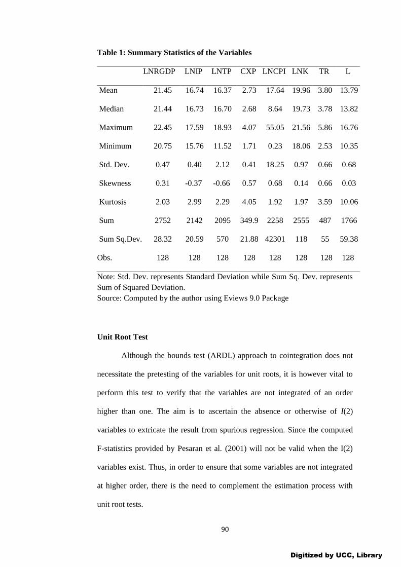
90

Table 1: Summary Statistics of the Variables

LNRGDP LNIP LNTP CXP LNCPI LNK TR L

Mean 21.45 16.74 16.37 2.73 17.64 19.96 3.80 13.79

Median 21.44 16.73 16.70 2.68 8.64 19.73 3.78 13.82

Maximum 22.45 17.59 18.93 4.07 55.05 21.56 5.86 16.76

Minimum 20.75 15.76 11.52 1.71 0.23 18.06 2.53 10.35

Std. Dev. 0.47 0.40 2.12 0.41 18.25 0.97 0.66 0.68

Skewness 0.31 -0.37 -0.66 0.57 0.68 0.14 0.66 0.03

Kurtosis 2.03 2.99 2.29 4.05 1.92 1.97 3.59 10.06

Sum 2752 2142 2095 349.9 2258 2555 487 1766

Sum Sq.Dev. 28.32 20.59 570 21.88 42301 118 55 59.38

Obs. 128 128 128 128 128 128 128 128

Note: Std. Dev. represents Standard Deviation while Sum Sq. Dev. represents

Sum of Squared Deviation.

Source: Computed by the author using Eviews 9.0 Package

Unit Root Test

Although the bounds test (ARDL) approach to cointegration does not

necessitate the pretesting of the variables for unit roots, it is however vital to

perform this test to verify that the variables are not integrated of an order

higher than one. The aim is to ascertain the absence or otherwise of I(2)

variables to extricate the result from spurious regression. Since the computed

F-statistics provided by Pesaran et al. (2001) will not be valid when the I(2)

variables exist. Thus, in order to ensure that some variables are not integrated

at higher order, there is the need to complement the estimation process with

unit root tests.


91

For this reason, all the variables were examined by first inspecting

their trends graphically. From the graphs in Appendix A, all the variables are

non-stationary in levels. Nonetheless, the plots of all the variables in their first

differences show that the variables are stationary (Appendix B).

Moreover, the Augmented Dickey-Fuller (ADF) and Phillips-Perron

(PP) tests were applied to all variables in levels and in first difference in order

to formally establish their order of integration. In order to be sure of the order

of integration of the variables, the test was conducted with intercept and time

trend in the model. The optimal number of lags included in the test was based

on automatic selection by Schwarz-Bayesian Criterion (SBC) and Akaike

Information Criterion (AIC). The study used the P-values in the parenthesis to

make the unit root decision, (that is, rejection or acceptance of the null

hypothesis that the series contain unit root) which arrived at similar conclusion

with the critical values.

The results of ADF test for unit root with intercept and tend in the

model for all the variables are presented in Table 2. The null hypothesis is that

the series is non-stationary, or contains a unit root. The rejection of the null

hypothesis for the test is based on the MacKinnon (1991) critical values as

well as the probability values.

The unit root test results in Table 2 indicate that, the null hypothesis of

the presence of unit root for all the variables in their levels cannot be rejected

since the P-values of the ADF statistic are not statistically significant at any of

three conventional levels of significance. But, at first difference, all the

variables are stationary. This is because the null hypothesis of the presence of


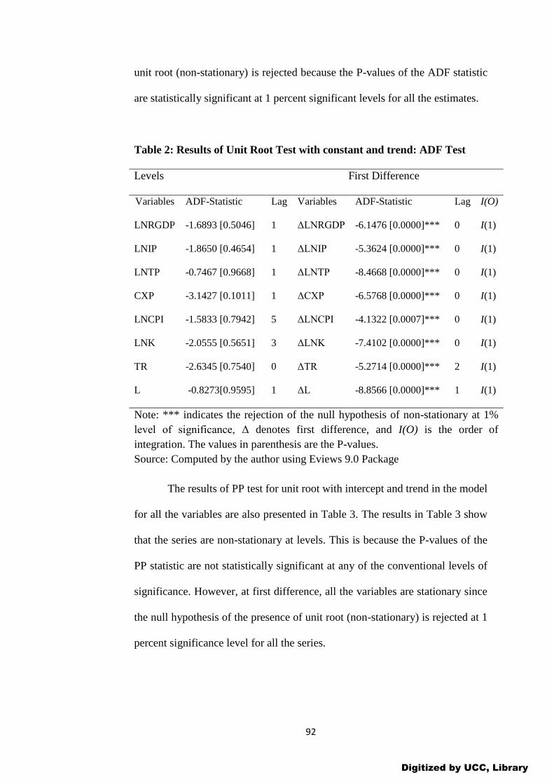
92

unit root (non-stationary) is rejected because the P-values of the ADF statistic

are statistically significant at 1 percent significant levels for all the estimates.

Table 2: Results of Unit Root Test with constant and trend: ADF Test

Levels First Difference

Variables ADF-Statistic Lag Variables ADF-Statistic Lag I(O)

LNRGDP -1.6893 [0.5046] 1 ΔLNRGDP -6.1476 [0.0000]*** 0 I(1)

LNIP -1.8650 [0.4654] 1 ΔLNIP -5.3624 [0.0000]*** 0 I(1)

LNTP -0.7467 [0.9668] 1 ΔLNTP -8.4668 [0.0000]*** 0 I(1)

CXP -3.1427 [0.1011] 1 ΔCXP -6.5768 [0.0000]*** 0 I(1)

LNCPI -1.5833 [0.7942] 5 ΔLNCPI -4.1322 [0.0007]*** 0 I(1)

LNK -2.0555 [0.5651] 3 ΔLNK -7.4102 [0.0000]*** 0 I(1)

TR -2.6345 [0.7540] 0 ΔTR -5.2714 [0.0000]*** 2 I(1)

L -0.8273[0.9595] 1 ΔL -8.8566 [0.0000]*** 1 I(1)

Note: *** indicates the rejection of the null hypothesis of non-stationary at 1%

level of significance, Δ denotes first difference, and I(O) is the order of

integration. The values in parenthesis are the P-values.


The results of PP test for unit root with intercept and trend in the model

for all the variables are also presented in Table 3. The results in Table 3 show

that the series are non-stationary at levels. This is because the P-values of the

PP statistic are not statistically significant at any of the conventional levels of

significance. However, at first difference, all the variables are stationary since

the null hypothesis of the presence of unit root (non-stationary) is rejected at 1

percent significance level for all the series.


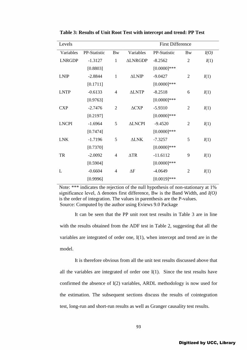
93

Table 3: Results of Unit Root Test with intercept and trend: PP Test

Levels First Difference

Variables PP-Statistic Bw Variables PP-Statistic Bw I(O)

LNRGDP -1.3127

[0.8803]

1 ΔLNRGDP -8.2562

[0.0000]***

2 I(1)

LNIP -2.8844

[0.1711]

1 ΔLNIP -9.0427

[0.0000]***

2 I(1)

LNTP -0.6133

[0.9763]

4 ΔLNTP -8.2518

[0.0000]***

6 I(1)

CXP -2.7476

[0.2197]

2 ΔCXP -5.9310

[0.0000]***

2 I(1)

LNCPI -1.6964

[0.7474]

5 ΔLNCPI -9.4520

[0.0000]***

2 I(1)

LNK -1.7196

[0.7370]

5 ΔLNK -7.3257

[0.0000]***

5 I(1)

TR -2.0092

[0.5904]

4 ΔTR -11.6112

[0.0000]***

9 I(1)

L -0.6604

[0.9996]

4 ΔF -4.0649

[0.0019]***

2 I(1)

Note: *** indicates the rejection of the null hypothesis of non-stationary at 1%

significance level, Δ denotes first difference, Bw is the Band Width, and I(O)

is the order of integration. The values in parenthesis are the P-values.


It can be seen that the PP unit root test results in Table 3 are in line

with the results obtained from the ADF test in Table 2, suggesting that all the

variables are integrated of order one, I(1), when intercept and trend are in the

model.

It is therefore obvious from all the unit test results discussed above that

all the variables are integrated of order one I(1). Since the test results have

confirmed the absence of I(2) variables, ARDL methodology is now used for

the estimation. The subsequent sections discuss the results of cointegration

test, long-run and short-run results as well as Granger causality test results.


94

Bounds Test for Cointegration

In the first step of the ARDL analysis, the presence of long-run

relationships in equation (14) is tested. Given that the study employed

quarterly data, a maximum lag length of 4 is used in the bounds test. Pesaran

and Pesaran (1997) suggest a maximum lag length of 4 for quarterly data in

the bounds testing approach to cointegration. After the lag length was

determined, the F-test statistic computed within the bounds test framework is

compared with the upper and lower critical values in Pesaran and Pesaran

(1997). The results of the bound test procedure for cointegration analysis for

some government expenditure components and economic growth are

presented in Table 4.

As shown in Table 4, the joint null hypothesis of lagged level variables

(that is, variable addition test) of the coefficients being zero (no cointegration)

is rejected at 1 percent significance level. This is because the calculated F-

statistic value of 4.664 (F LNRGDP (.)= 4.664) exceeds the upper bound critical

value of 4.540 at 99% level. This means there exist a long run relationship

between government expenditure components and economic growth.

Table 4: Results of Bounds Tests for the Existence of Cointegration

90% Level 95% Level 99% Level

K I(0) I(1) I(0) I(1) I(0) I(1)

7 2.141 3.250 2.476 3.646 3.267 4.540

Dependent Variable F-Statistic

F(LNRGDP) = F (LNRGDP|LNIP, LNTP, CXP, LNCPI,

LNK, TR, L)

4.664

Note: Critical values were obtained from Pesaran and Pesaran (1997),

Appendix C, Table F, pp. 478, and K is the number of regressors.

Source: Computed by the author using Microfit 4.1 package.


95

The results in Table 4 indicate that there is a unique cointegration

relationship among the variables when economic growth is normalized.

Hence, there is a long-run relationship between economic growth and the

explanatory variables in Ghana.

Having established the existence of long-run relationship between the

explanatory variables and economic growth in the model and an error

correction mechanism exists, the ARDL cointegration method is used to

estimate the long-run coefficients and the short-run parameters of equation

(14).

Long Run Relationship

This section highlights the long-run estimation results which addressed

the study’s objective of a long-run relationship between government

expenditure components and economic growth in Ghana. The analysis tests

the null hypothesis of no long run relationship between government

expenditure components and economic growth as against the alternative

hypothesis of a long run relationship between government expenditure

components and economic growth. Based on the results, the null hypothesis of

no long-run relationship between the variables was rejected.

In view of the fact that government expenditure components and

economic growth are cointegrated, the long-run parameters of the ARDL

model are estimated and the results are presented in the Table 5. The long-run

ARDL model was estimated based on the Schwarz Bayesian Criterion (SBC)

in order to ensure that the results are parsimonious.


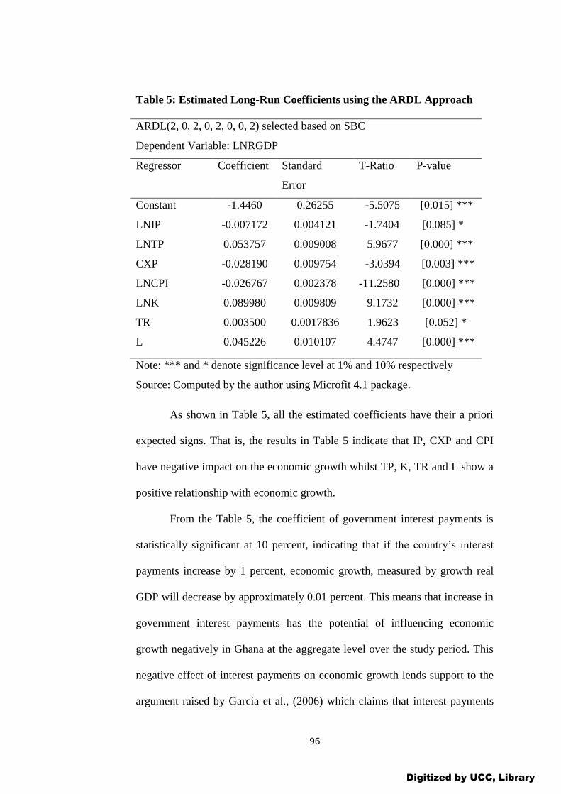
96

Table 5: Estimated Long-Run Coefficients using the ARDL Approach

ARDL(2, 0, 2, 0, 2, 0, 0, 2) selected based on SBC

Dependent Variable: LNRGDP

Regressor Coefficient

Standard

Error

T-Ratio

P-value

Constant -1.4460 0.26255 -5.5075 [0.015] ***

LNIP -0.007172 0.004121 -1.7404 [0.085] *

LNTP 0.053757 0.009008 5.9677 [0.000] ***

CXP -0.028190 0.009754 -3.0394 [0.003] ***

LNCPI -0.026767 0.002378 -11.2580 [0.000] ***

LNK 0.089980 0.009809 9.1732 [0.000] ***

TR

L

0.003500

0.045226

0.0017836

0.010107

1.9623

4.4747

[0.052] *

[0.000] ***

Note: *** and * denote significance level at 1% and 10% respectively


As shown in Table 5, all the estimated coefficients have their a priori

expected signs. That is, the results in Table 5 indicate that IP, CXP and CPI

have negative impact on the economic growth whilst TP, K, TR and L show a

positive relationship with economic growth.

From the Table 5, the coefficient of government interest payments is

statistically significant at 10 percent, indicating that if the country’s interest

payments increase by 1 percent, economic growth, measured by growth real

GDP will decrease by approximately 0.01 percent. This means that increase in

government interest payments has the potential of influencing economic

growth negatively in Ghana at the aggregate level over the study period. This

negative effect of interest payments on economic growth lends support to the

argument raised by García et al., (2006) which claims that interest payments


97

impact on long-run economic growth negatively due to their crowding-out

effects on other productive expenditures. Hence, high interest payments are

associated with changes in economic growth which has the potential of

decreasing economic activities of both public and private sectors of the

economy. The implication is that, resources which could have been used to

acquire capital assets are used to defray interest burden which adversely

impacts the growth of output. The impact of interest payments on growth

becomes more severe when government has to pay the interest through taxes.

Thus, increase in taxes could reduce households’ disposable income and

returns on investment; increase cost of production and eventually increase

general price levels. All these ultimately result in a fall in aggregate demand

and output.

Furthermore, the coefficient of government transfer payments carried

the expected positive sign and is statistically significant at 1 percent

significance level. This indicates that, if the government transfer payments

increases by 1 percent, then real gross domestic product (economic growth)

will increase by approximately 0.054 percent in the long-run (as indicated in

Table 5). This result is in line with the Keynesian hypothesis which argues that

government transfer payments are crucial for economic growth and that high

transfer payments improve long-term economic growth of a country.

Moreover, the result also confirms most findings of empirical studies

in the literature. Particularly, it agrees with studies by Twumasi (2012);

Afonso and Furceri (2008) who found a positive effect of government transfer

payments on economic growth for the EU countries. Such long-run positive

impact of government transfer payments on economic growth could be


98

attributed to the positive impact of transfer payments on households’

disposable incomes which increases their purchasing power and the ability to

develop their human resource.

Additionally, it can be observed from Table 5 that, the coefficient of

government consumption expenditure in the long-run estimation results is

negative (-0.02819) and statistically significant at 1 percent significance level.

The implication of the coefficient is that, a 1 percentage increase in the general

government final consumption expenditure as a percentage of GDP will cause

real GDP (economic growth) to decrease by approximately 0.03 percent in the

long-run. The negative sign associated with the government consumption

expenditure confirms the theoretical thought that suggests that an increase in

government consumption expenditure retards the economy’s steady state

growth. The negative impact could be justified by the crowding-out effect

which is generally associated with government consumption expenditure and

mainly how such expenditures are financed (taxes and borrowing).

In Ghana, despite the fact that government consumption expenditure

has been essential to the welfare of the economy, it has not proven to be

productive when economic growth is considered (Twumasi, 2012). The result

further confirms the findings of empirical studies in the literature by Barro

(1989) using 98 developed and developing countries; Afonso and Alegre

(2008) using 27 EU countries; Afonso and Furceri (2008) with data from

OECD and EU countries; (Agalega & Acheampong, n.d.) using data from

Ghana. The results of these studies indicated a negative effect of government

consumption expenditure on economic growth for the countries concerned.

However, this finding contradicts that of Ocran (2011) who found a significant


99

positive relationship between government consumption expenditure and

economic growth in South Africa.

In addition, the coefficient of consumer price index (CPI) is negative in

sign and is statistically significant at 1 percent significance level. The

coefficient indicates that a 1 percentage increase in the general price levels

will induce economic growth to fall by approximately 0.027 percent in the

long-run. The implication here is that, price stability of an economy is an

indispensable element in achieving economic growth. The reason is that

inflation impedes domestic demand and escalates the cost of production

thereby decelerating the rate of growth of the economy. This result reaffirms

the finding of Frimpong et al., (2006) who found a significant and negative

connection between general price levels and economic growth in Ghana.

The result further supports that of Gokal and Hanif (2004); Ahmed and

Mortaza (2005); Georgantopoulous and Tsamis (2012) who indicated a

statistically significant long run inverse relationship between inflation and

economic growth. On the contrary, Mallik and Chowdhury (2001) highlighted

a positive relationship between economic growth and inflation for Bangladesh,

India, Pakistan and Sri Lanka.

As expected, from Table 5, the coefficient of physical capital stock (as

measured by gross fixed capital formation) is positive and statistically

significant at 1 percent. This indicates that, if the country’s stock of capital

goes up by 1 percent, holding all other things constant, economic growth will

increase by approximately 0.090 percent in the long run. This means that

physical capital stock contributes positively to economic growth in the long-

run in Ghana. This direct correlation is consistent with the classical economic


100

theory, and supports the claim made by Yasin (2003); Fosu and Aryeetey

(2008) Alexiou (2009); Ocran (2011) that growth of gross fixed capital

formation impacts output growth positively.

Further, the coefficient of tax revenue has the expected positive sign,

and statistically significant at 10 percent. This means that when government

tax revenue (as a percentage of GDP) increases by 1 percent, economic growth

will increase by approximately 0.004 percent in the long run in Ghana. The

justification for this positive relationship between tax revenue and economic

growth is that, government revenue generated through taxation can be used to

finance its capital expenditure and transfer payments which ultimately results

in growth of output of the economy. This finding favours the argument by

Mullen and Williams (1994); Ocran (2011); Ogbonna and Ebimobowei (2012)

Antwi et al., (2013) who established significant and a positive relationship

between economic growth and tax revenue.

The coefficient of labour force (Population aged 15-64 years as a

percentage total population) also has its expected positive sign and is

statistically significant at 1 percent significance level. This means that if

labour force increases by 1 percent, economic growth will also increase by

approximately 0.05 percent in the long run, holding all other things constant,

in Ghana. What ought to be emphasized here is that, a mere increase in labour

force could not lead to the desired growth of output hence the labour force

must be equipped with the required stills and expertise to be able to make this

positive relationship with output growth a reality. This result supports the

view of Frimpong et al., (2006) who indicated that, labour is important in

explaining economic growth in the long run in Ghana.


101

Again, the finding confirms the emphasis made by Wilkins (2004);

Jayaraman and Singh (2007); Ogundipe and Oluwatobi (2013) who argued

that there is a positive and significant relationship between labour force and

economic growth since economic growth cannot be achieved without labour as

an input of production. M’Amanja and Morrisey (2005) also highlighted a

positive relationship between labour force and economic growth.

Short Run Relationship

This section presents the estimation results of the short-run relationship

between economic growth and government expenditure components in Ghana.

The analysis was meant to test the null hypothesis of no short-run relationship

between economic growth and the government expenditure components as

against the alternative hypothesis of a short-run relationship between

economic growth and government expenditure components. The results in

Table 6 indicate that all variables are statistically significant, therefore the null

hypothesis of no short-run relationship between the variables was rejected.

Once the long-run cointegrating model has been estimated, the next

step is to model the short-run dynamic relationship among the variables within

the ARDL framework. Consequently, the lagged value of all level variables (a

linear combination) is denoted by the error-correction term, ECMt-1, is retained

in the ARDL model.

Table 6 presents the results of the estimated error-correction model of

economic growth for Ghana using the ARDL framework. The model is

selected based on the SBC.


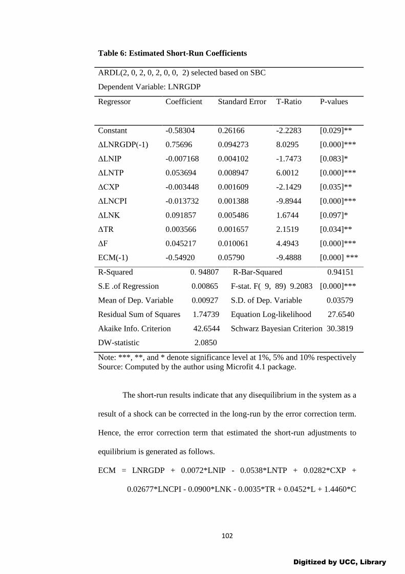
102

Table 6: Estimated Short-Run Coefficients

ARDL(2, 0, 2, 0, 2, 0, 0, 2) selected based on SBC

Dependent Variable: LNRGDP

Regressor Coefficient

Standard Error

T-Ratio

P-values

Constant -0.58304 0.26166 -2.2283 [0.029]**

ΔLNRGDP(-1) 0.75696 0.094273 8.0295 [0.000]***

ΔLNIP -0.007168 0.004102 -1.7473 [0.083]*

ΔLNTP 0.053694 0.008947 6.0012 [0.000]***

ΔCXP -0.003448 0.001609 -2.1429 [0.035]**

ΔLNCPI -0.013732 0.001388 -9.8944 [0.000]***

ΔLNK 0.091857 0.005486 1.6744 [0.097]*

ΔTR

ΔF

0.003566

0.045217

0.001657

0.010061

2.1519

4.4943

[0.034]**

[0.000]***

ECM(-1) -0.54920 0.05790 -9.4888 [0.000] ***

R-Squared 0. 94807 R-Bar-Squared 0.94151

S.E .of Regression 0.00865 F-stat. F( 9, 89) 9.2083 [0.000]***

Mean of Dep. Variable 0.00927 S.D. of Dep. Variable 0.03579

Residual Sum of Squares 1.74739 Equation Log-likelihood 27.6540

Akaike Info. Criterion 42.6544 Schwarz Bayesian Criterion 30.3819

DW-statistic 2.0850

Note: ***, **, and * denote significance level at 1%, 5% and 10% respectively


The short-run results indicate that any disequilibrium in the system as a

result of a shock can be corrected in the long-run by the error correction term.

Hence, the error correction term that estimated the short-run adjustments to

equilibrium is generated as follows.

ECM = LNRGDP + 0.0072*LNIP - 0.0538*LNTP + 0.0282*CXP +

0.02677*LNCPI - 0.0900*LNK - 0.0035*TR + 0.0452*L + 1.4460*C


103

The results from the ARDL model as displayed in Table 6 suggest that

the ultimate effect of previous period value of economic growth on current

values of economic growth in the short-run is positive and statistically

significant at 1 percent significant level. The implication is that current values

of economic growth are affected by previous quarters’ values of economic

growth in Ghana. This is expected in that previous growth and expansion in

the growth of the economy serves as an indication of prosperity and may

attract more investment leading to more growth.

The results also showed the expected negative sign of error correction

term lagged one period (ECMt-1) and it is highly significant at 1 percent

significance level. This confirms the existence of the cointegration relationship

among the variables (that is economic growth and government expenditure

components) in the model. The Error Correction Term (ECT) stands for the

speed of adjustment to restore equilibrium in the dynamic model following a

disturbance. The coefficient of the error correction term (ECM) is -0.54920.

This suggests that, about 55 percent of the deviations from the long term

output growth caused by previous quarter’s shocks converge back to the long

run equilibrium in the current quarter of the year. The rule of thumb is that, the

larger the error correction coefficient (in absolute terms), the faster the

variables equilibrate in the long-run when shocked in the previous period

(Acheampong, 2007; Oyinlola & Akinnibosun, 2013).

Consistent with the long-run results, the coefficient of interest

payments has the theorized negative impact on economic growth in the short-

run. Thus, the coefficient is statistically significant at 10 percent. From the

results in Table 6, a 1 percentage point increase in interest payments will cause


104

economic growth to decrease by approximately 0.007 percent in the short-run.

This indicates the crucial role that interest payments on loans play in Ghana’s

growth process as its coefficient is negative in the dynamic model just as in

the long run model. This result is in harmony with that of Garcia et al. (2006)

who found a significant and negative relationship between government interest

payments and economic growth in Chile. This relationship can be attributed to

the crowding-out effects of interest payments on private investments and other

productive spending.

Again, the coefficient of government transfer payments also

maintained its positive sign and statistically significant at 1 percent significant

level which is consistent with the long-run results. The result therefore implies

that, if government transfer payments go up by 1 percent, economic growth

accordingly will increase by approximately 0.054 percent in the short-run.

Thus, the short-run and long-run results indicate that government transfer

payments have been favourable for economic growth in Ghana over the period

under study.

Furthermore, consistent with the long-run findings in Table 5, the

coefficient of government consumption expenditure maintained its negative

sign and statistically significant at 5 percent significance level in the short-run.

This means that in the short-run, if the government consumption expenditure

increases by 1 percent, economic growth will decrease by approximately 0.003

percent, which is less than the long-run coefficient of 0.028 percent. This

shows how important it is to deal with high government consumption

expenditure in relation to growth in the Ghanaian economy.


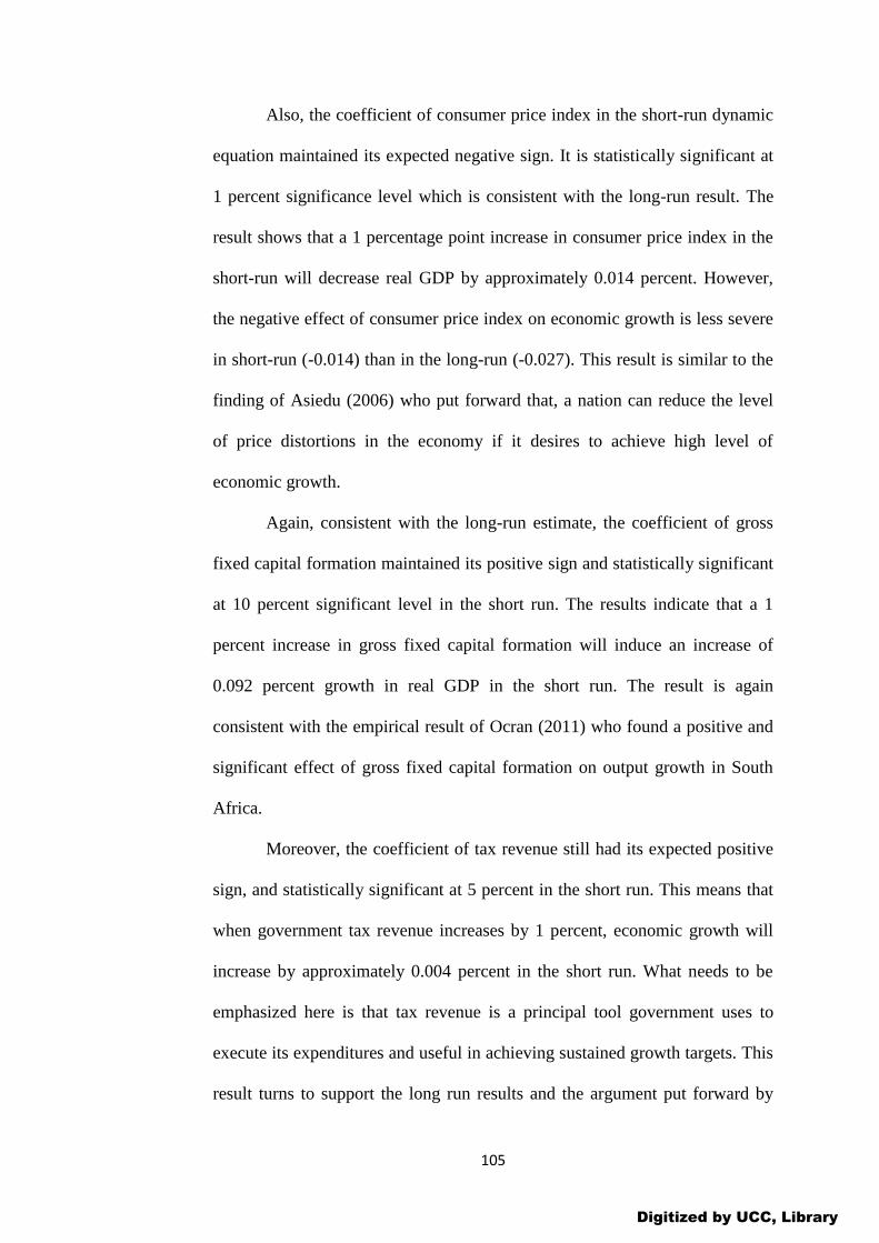
105

Also, the coefficient of consumer price index in the short-run dynamic

equation maintained its expected negative sign. It is statistically significant at

1 percent significance level which is consistent with the long-run result. The

result shows that a 1 percentage point increase in consumer price index in the

short-run will decrease real GDP by approximately 0.014 percent. However,

the negative effect of consumer price index on economic growth is less severe

in short-run (-0.014) than in the long-run (-0.027). This result is similar to the

finding of Asiedu (2006) who put forward that, a nation can reduce the level

of price distortions in the economy if it desires to achieve high level of

economic growth.

Again, consistent with the long-run estimate, the coefficient of gross

fixed capital formation maintained its positive sign and statistically significant

at 10 percent significant level in the short run. The results indicate that a 1

percent increase in gross fixed capital formation will induce an increase of

0.092 percent growth in real GDP in the short run. The result is again

consistent with the empirical result of Ocran (2011) who found a positive and

significant effect of gross fixed capital formation on output growth in South

Africa.

Moreover, the coefficient of tax revenue still had its expected positive

sign, and statistically significant at 5 percent in the short run. This means that

when government tax revenue increases by 1 percent, economic growth will

increase by approximately 0.004 percent in the short run. What needs to be

emphasized here is that tax revenue is a principal tool government uses to

execute its expenditures and useful in achieving sustained growth targets. This

result turns to support the long run results and the argument put forward by


106

Mullen and Williams (1994); Ocran (2011); Ogbonna and Ebimobowei (2012)

that tax revenue has significant and a positive effect on real GDP. However,

this result conflicts with that of Dackehag and Hansson (2012) who found a

negative relationship between tax revenue and economic growth. This

negative relationship is explained by the distortions that raising tax revenues

cause on economic activities. Worlu and Nkoro (2012) also found no

significant relationship between tax revenue and economic growth in Nigeria.

Labour force had the expected positive sign as in the long-run results.

Thus, its coefficient is statistically significant at 1 percent significance level in

the short run. This implies that as labour force in the country increases by 1

percent, holding all other things constant, economic growth will increase by

0.045 percent in the short run.

With the R-Square value of 0.94807 suggests that about 95 percent of

the variations in economic growth are explained by the regressors in the

model.

Lastly, on the differential effect of government expenditure

components, the results in Table 5 indicates that, among government

consumption expenditure, transfer and interest payments, only transfer

payment was found to stimulate growth by 0.054% for every 1 percentage

point increase in transfer payment. Government consumption and interest

payments, on the other hand, were found to retard growth of output by 0.028%

and 0.007% when each of these expenditure components increases by 1

percent respectively in the long run. These results are not significantly

different from the short run results in Table 6.


107

Model Diagnostics and Stability Tests

In order to check for the estimated ARDL model, the significance of

the variables and other diagnostic tests such as serial correlation, functional

form, normality, heteroskedasticity and structural stability of the model are

considered. As shown in Table 7, the model generally passes all diagnostic

tests in the first stage. The diagnostic test shows that there is no evidence of

autocorrelation and the model passes the normality and the test proved that the

error term is normally distributed. Additionally, the model passes the white

test for heteroskedasticity as well as the RESET test for correct specification

of the model.

Table 7: Model Diagnostics

Diagnostics Test Statistic(P-Value)

FAuto (4,80) 1.6885 [0.158]

X2Auto (4) 7.5473 [0.110]

X2Reset (1) 0.1530 [0.696]

X2Norm (2) 1.5794 [0.404]

X2White (1) 8.3370 [0.842]

Note: X2Auto, X2

Reset, X2

Norm, and X2White are Lagrange multiplier statistics for

test of serial correlation, functional form misspecification, non-normal errors

and heteroskedasticity respectively. These statistics are distributed as Chi-

square values with degree of freedom in parentheses. Values in parentheses [ ]

are probability values.


Finally, when analyzing the stability of the coefficients, the

Cumulative Sum (CUSUM) and Cumulative Sum of Squares (CUSUMQ) are

applied. Following Pesaran and Pesaran (1997); Bahmani-Oskooee and Nasir,

2004), the stability of the regression coefficients is evaluated by stability tests


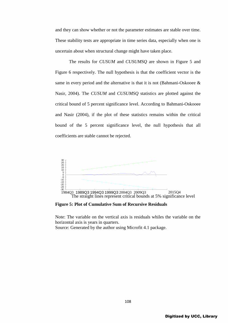
108

and they can show whether or not the parameter estimates are stable over time.

These stability tests are appropriate in time series data, especially when one is

uncertain about when structural change might have taken place.

The results for CUSUM and CUSUMSQ are shown in Figure 5 and

Figure 6 respectively. The null hypothesis is that the coefficient vector is the

same in every period and the alternative is that it is not (Bahmani-Oskooee &

Nasir, 2004). The CUSUM and CUSUMSQ statistics are plotted against the

critical bound of 5 percent significance level. According to Bahmani-Oskooee

and Nasir (2004), if the plot of these statistics remains within the critical

bound of the 5 percent significance level, the null hypothesis that all

coefficients are stable cannot be rejected.

Note: The variable on the vertical axis is residuals whiles the variable on the

horizontal axis is years in quarters.

Source: Generated by the author using Microfit 4.1 package.

The straight lines represent critical bounds at 5% significance level 2009Q3 2015Q4

-5 -10 -15 -20 -25 -30

0 5

10 15 20 25 30

1984Q3 1989Q3 1994Q3 1999Q3 2004Q3

Figure 5: Plot of Cumulative Sum of Recursive Residuals


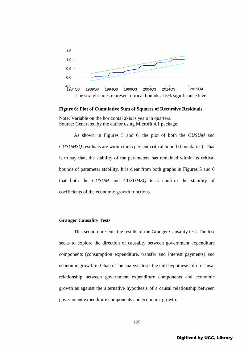
109

Note: The variable on the vertical axis is the square of the residuals whiles the

Note: Variable on the horizontal axis is years in quarters.

Source: Generated by the author using Microfit 4.1 package.

As shown in Figures 5 and 6, the plot of both the CUSUM and

CUSUMSQ residuals are within the 5 percent critical bound (boundaries). That

is to say that, the stability of the parameters has remained within its critical

bounds of parameter stability. It is clear from both graphs in Figures 5 and 6

that both the CUSUM and CUSUMSQ tests confirm the stability of

coefficients of the economic growth functions.

Granger Causality Tests

This section presents the results of the Granger Causality test. The test

seeks to explore the direction of causality between government expenditure

components (consumption expenditure, transfer and interest payments) and

economic growth in Ghana. The analysis tests the null hypothesis of no causal

relationship between government expenditure components and economic

growth as against the alternative hypothesis of a causal relationship between

government expenditure components and economic growth.

The straight lines represent critical bounds at 5% significance level

-0.5

0.0

0.5

1.0

1.5

1984Q3 1989Q3 1994Q3 1999Q3 2004Q3 2014Q3 2015Q4

Figure 6: Plot of Cumulative Sum of Squares of Recursive Residuals


110

Having established cointegration among the variables, Granger

causality test was then applied to measure the linear causation between

government expenditure components and economic growth.

The results of the Pair-wise granger causality test is presented in Table

8. The results in Table 8 suggest that the null hypothesis that government

interest payment does not granger-cause economic growth is rejected at 5

percent significance level. This means that government interest payment

granger-causes economic growth in Ghana.

Moreover, the null hypothesis that economic growth does not granger-

cause government interest payment is also rejected at 5 percent significance

level implying that economic growth also granger-causes interest payment

suggesting a bidirectional causality between government interest payment and

economic growth in Ghana.

Table 8: Results of Pair-wise Granger Causality Tests

Null Hypothesis F-Stat. Prob. Remarks

LNIP does not Granger Cause LNRGDP 3.36650 0.0355** Reject H0

LNRGDP does not Granger Cause LNIP 4.72317 0.0106** Reject H0

CXP does not Granger Cause LNRGDP

LNRGDP does not Granger Cause CXP

LNTP does not Granger Cause LNRGDP

LNRGDP does not Granger Cause LNTP

3.87459

0.65257

4.98115

2.25144

0.0234**

0.5225

0.0083***

0.1096

Reject H0

Accept H0

Reject H0

Accept H0

Note: *** and ** denote significance level at 1% and 5% respectively.

Source: Estimated by the author using E-views 9.0 package.


111

Furthermore, the results in Table 8 indicate that the null hypothesis that

government consumption expenditure does not granger-cause economic

growth is rejected at 5 percent significance level. This means that government

consumption expenditure granger-causes economic growth in Ghana, but not

economic growth granger-causing government consumption expenditure. This

indicates a unidirectional causality running from government consumption

expenditure to economic growth.

Lastly, it can be observed from Table 8 that the null hypothesis that

government transfer payment does not granger-cause economic growth is

rejected at 1 percent significance level. But the null hypothesis that economic

growth granger-causes government transfer payment is accepted. This implies

that government transfer payment granger-causes economic growth, and that

there is a unidirectional causality running from government transfer payment

to economic growth in Ghana.

Conclusion

This chapter examined the time series properties of the data used for

estimation, presented and discussed the results. Unit root tests employing both

the ADF and the PP techniques essentially show that all the series had to be

differenced once to achieve stationarity. This means that all the series are

integrated of order one, I(1). The presence of non-stationary variables implied

the possibility of the presence of a long-run relationship among the variables,

which the study verified using ARDL bounds test approach. The results show

the presence of long-run and short-run relationship between government

expenditure components and economic growth in Ghana. Whereas


112

government transfer payment was found have a positive and statistically

significant impact on economic growth, government interest payment and

consumption expenditure indicated negative significant effect on output

growth. The results further show that tax revenue, physical capital stock and

labour force positively influence economic growth. Lastly, consumer price

index exhibited a significant negative relationship with economic growth for

the study period.

The results of the ARDL (2, 0, 2, 0, 2, 0, 0, 2) model selected based on

SBC show that the error correction term (ECMt-1) for economic growth carried

the expected negative sign. Also, the results imply that the variables play a

significant role in explaining economic growth in Ghana. The coefficients for

all the explanatory variables were well behaved and had the expected signs

and they were significant both in the long-run and short-run.

The diagnostic and parameter stability tests revealed that the model

passes the tests of serial correlation, functional form misspecification, non-

normal errors and heteroskedasticity at conventional levels of significance and

the graphs of the CUSUM and CUSUMSQ indicate the absence of any

instability of the coefficients because the plots of these graphs are confined

within the 5 percent critical bounds of parameter stability suggesting that all

the coefficients of the estimated ARDL (2, 0, 2, 0, 2, 0, 0, 2) model are stable

over the study period.

The Granger causality test results revealed a bi-directional causality

between economic growth and government interest payment in Ghana. The

results further indicated a unidirectional causality running from both


113

government consumption expenditure and government transfer payment to

economic growth in Ghana.


114

CHAPTER FIVE

SUMMARY, CONCLUSIONS AND RECOMMENDATIONS

Introduction

The chapter presents the summary, conclusions and recommendations

of the study. Whilst the summary presents a brief overview of the research

problem, objectives, methodology and findings, the conclusions highlight the

overall outcomes regarding the findings of the study in light of the hypotheses,

and the recommendations provide specific remedies to be implemented by

particular agencies. The chapter further provides the limitations of the study

and direction for future research.

Summary

This study investigated the growth impact of government consumption,

transfer and interest payments in Ghana using quarterly time series data from

1984-2015. The investigation was done by regressing economic growth,

proxied by real GDP, government interest payments, government transfer

payments, government consumption expenditure, tax revenue, consumer price

index, capital stock and labour force in an Autoregressive Distributed Lag

(ARDL) model. The study specifically examined the long-run and short-run

relationships among the variables in Ghana. The ARDL approach to

cointegration was employed to examine the long-run and short-run dynamics

among the variables in the estimation. All tests and estimations were

conducted using E-views 9.0 and Microfit 4.1 package.

The first step in the estimation process involved testing for the

stationarity properties of the variables using both the Augmented-Dickey


115

Fuller (ADF) and Phillips-Perron (PP) test statistics. The unit roots results

suggest that all the variables were stationary after taking the first difference.

Secondly, the study proceeded to examine the long-run and short-run

relationships between government expenditure components and economic

growth using the maximum likelihood based approach within ARDL approach

to cointegration proposed by Pesaran and Shin (1999). Third, the assessment

of the diagnostic and stability test statistics revealed that the estimated model

was satisfactory in line with the Lagrange multiplier and F-statistic. The plots

of the cumulative sum of recursive residuals and the cumulative sum of

squares of recursive residual stability test for the model indicated that all the

parameters estimated were stable over the study period since they were found

to be within the five percent critical bounds level. Lastly, the study further

proceeded to examine the causal relationship between the government

expenditure components considered and economic growth using the pair-wise

Granger-causality test. The following are therefore the findings of the study:

The cointegration analysis revealed the presence of long-run

relationship among economic growth, government interest payments,

government transfer payments, government consumption expenditure,

consumer price index, gross fixed capital formation, tax revenue and labour

force.

The error correction model also revealed a short run relationship

among the variables. It can be said that, the results in the short-run were

consistent with the results in the long-run. The positive and negative effects

of most of the variables on economic growth were bigger in magnitude in the

long-run than in the short-run.


116

The results from the ARDL model estimation indicated that, among the

government expenditure components considered, only government transfer

payments was found to have a significant positive relationship with

economic growth. Government interest payments and consumption

expenditure revealed negative and significant impact on economic growth in

both short-run and long-run. Consumer price index was found to have

negative effect on growth. However, capital stock, tax revenue and labour

force show positive and significant effect on economic growth. It must be

noted that, the short run results confirm the long run results, but the

magnitudes of the impact (coefficients) of the regressors in the long run are

bigger than in the short run for the study period. Additionally, the existence

of a long-run relationship among the variables was further confirmed by the

negative and statistically significant coefficient of the lagged error correction

term. The value of the coefficient suggests that about 55 percent of the

disequilibrium caused by previous quarters’ shocks converges back to the

long-run equilibrium in the current quarter in each year. Statistically, any

disequilibrium in the Ghanaian economy takes about seven months to restore

to equilibrium.

The diagnostic tests results show that the model passes the test of serial

correlation, functional form misspecification, non-normal errors and

heteroscedasticity at conventional levels of significance. The graphs of the

cumulative sum of recursive residuals (CUSUM) and the cumulative sum of

squares of recursive residuals (CUSUMSQ) show that there is stability of the

parameters.


117

Lastly, the Granger-causality test was carried on the government

expenditure components (government consumption, transfer and interest

payments) and economic growth.

Conclusions

The principal objective of this study was to investigate the growth

impact of government consumption, transfer and interest payments in Ghana.

Investigation of the relationship between government expenditure components

and economic growth has become a subject of interest for many researchers.

The reason is the mounting evidence that indicates that stability of

macroeconomic variables leads to economic growth. The analysis of

government expenditure-economic growth nexus has captured the interest of

development practitioners, finance experts, and researchers as well as policy

makers in recent times given the turbulent experiences of the world economy

and its accompanying consequences. The study therefore investigated the

growth impact of government consumption, transfer and interest payments in

Ghana. The study made emphasis on two key issues: the relationship between

government expenditure components and economic growth; and the direction

of causality between government expenditure components and economic

growth. Considering the results of the study, the following conclusions were

drawn.

The study in line with the empirical literature has shown that there

exists a long-run and short-run relationship among variables of interest,

particularly government transfer payments, physical capital stock, tax revenue


118

and labour force were found to have positive effects on the growth of output in

both short run and long run in Ghana. The implication is that increase in the

volume of transfer payments, capital stock and tax revenue together with

growth of labour force will cause the Ghanaian economy to growth in both

short run and long run.

Again, the results presented in this study imply that government

interest payments, government consumption expenditure and consumer price

index are also statistically important determinants of economic growth but

have a negative relationship with output growth, both in the long-run and in

the short-run.

Finally, the study found a bi-directional causality between economic

growth and government interest payment. Unidirectional causalities running

from government consumption expenditure and transfer payment to economic

growth were also indicated.

Recommendations

Based on the findings from the study, the following recommendations

are proposed.

Government of Ghana through the Ministry of finance has taken

measures to mitigate the upsurge of interest payment in government

expenditure. These measures include interest rate hedging through swap

management, and government managing to pay its loan within the stipulated

period. To ensure the effectiveness of these policies, the Ministry of Finance

should ensure that the loans are used to finance projects that can generate

income within a reasonable period to pay off the debts. Lastly, the Ministry of


119

Finance should establish an institution whose responsibility will be to track

and ensure that any fund government releases is used for the intended project,

and demand comprehensive account on each project.

Government through the Ministry of Finance should take measures

toward reducing its consumption expenditures, more importantly on those that

are likely to have crowding-out effects on the economy. That is, the

consumption expenditures which are financed through domestic borrowing.

Again, the Ministry of Finance should ensure that much of government

consumption expenses are made on domestically produced goods in order to

increase aggregate demand and output that will culminate in long term growth

of the economy.

Moreover, the study recommends that government through the

Livelihood Empowerment Against Poverty (LEAP) programme under the

Department of Social Welfare should increase and regularize its transfer

payments in order to elevate the vulnerable groups from extreme poverty.

Lastly, the study recommends that the Ministry of Finance should take

measures that will bring about efficiency in the tax system in the country.

Specifically, the ministry should ensure that the tax base is widened while

keeping the tax rate low. The result of this is that tax evasion in the system

will be minimised, tax revenue will improve and real GDP will grow.

Limitations of the Study

The main limitation of the study has to do with the quality and limited

availability of quarterly data on key variables. To produce highly reliable


120

estimates particularly with cointegration variables that have their values

already in quarters was needed. Accordingly, quarterly series were generated

through interpolation for the purpose of the estimation. Nonetheless, there is

no gain in the power of these tests by switching from low frequency to high

frequency data and merely increasing the number of observations over a short

time period (Campbell & Perron, 1991). The utilization of interpolated

quarterly series did not, however, create danger to the reliability of the results

for the reason that Acheampong (2007); Anaman and Osei-Amponsah (2007)

used similar approach and arrived at reliable results.

The study examined the differential effects of government

consumption expenditure, transfer payments and interest payments on

economic growth. Some government expenditure components were not

included because Appiah (2014) has considered government capital

expenditure and recurrent expenditure, and others were due to data and time

constraint.

The study did not include human capital in the model because among

the focus was to ascertain the effect of the size of labour force on economic

growth but not the quality of labour force on output growth.

However, none of these limitations was found to have any effect on the

reliability of the results of the study as well as the conclusions and

recommendations from the study.

Direction for Future Research

The study examined the growth impact of government consumption,

transfer and interest payments in Ghana. The study could not consider the


121

connection between other government expenditure components (domestic

interest payments, external interest payments and compensation to employees)

and economic growth. Therefore, further study in this area can be carried to

investigate this relationship.


122

REFERENCES

Abdelal, R., Blyth, M., & Parsons, C. (2015). Constructing the international

economy. Cornell University Press.

Abu-Bader, S., & Abu-Qarn, A. S. (2003). Government expenditures, military

spending and economic growth: causality evidence from Egypt, Israel,

and Syria. Journal of Policy Modeling, 25(6), 567–583.

Acheampong, I. K. (2007). Testing Mckinnon-Shaw thesis in the context of

Ghana’s financial sector liberalisation episode. International Journal

of Management Research and Technology, 1(2), 156–183.

Adefeso, H. A., Hakeem, M., & Salawu, B. (2010). Fiscal Policy and

Economic Growth in Nigeria: Testing the Prediction of the

Endogenous Growth Model. The Social Sciences, 5(2), 96–102.

Adnan, A. (2014). The Impact of Public final consumption and investment

spending on Economic Growth in Ethiopia: An Application of Vector

Error Correction Model. AAU. Retrieved November 18, 2015 from

http://etd.aau.edu.et/handle/123456789/5089

Afonso, A., & Furceri, D. (2010). Government size, composition, volatility

and economic growth. European Journal of Political Economy, 26(4),

517–532.

Afonso, A., & Gonzalez Alegre, J. (2008). Economic growth and budgetary

components: a panel assessment for the EU. Retrieved September 11,

2015 from https://www.repository.utl.pt/handle/10400.5/2138

Agalega, E., & Acheampong, P. (n.d.). The Impact of Inflation, Policy Rate

and Government Consumption Expenditure on GDP Growth in Ghana:

A Co-Integration Approach. Retrieved July 28, 2015 from


123

http://pakacademicsearch.com/pdf-files/ech/517/184-

191%20Vol%205,%20No%2015%20(2013).pdf

Ahmed, S., & Mortaza, M. G. (2005). Inflation and growth in Bangladesh:

1981-2005. Policy Analysis Unit, Working Paper Series: WP, 604.

Aladejare, S. A. (2013). Government spending and economic growth:

evidence from Nigeria. MPRA Paper, 43916. Retrieved August 24,

2015 from http://core.ac.uk/download/pdf/12035238.pdf

Alexiou, C. (2009). Government spending and economic growth: Econometric

evidence from the South Eastern Europe (SEE). Journal of Economic

and Social Research, 11(1), 1-7

Al-Faris, A. F. (2002). Public expenditure and economic growth in the Gulf

Cooperation Council countries. Applied Economics, 34(9), 1187–1193.

Al-Fawwaz, T. M., & Al-Sawai’e, K. M. (2013). The relationship between

gross domestic product and government expenditures in Jordan: A

VAR Approach. Interdisciplinary Journal of Contemporary Research

in Business, 4(9), 336-244.

Amoako-Gyampah, K., & Acquaah, M. (2008). Manufacturing strategy,

competitive strategy and firm performance: An empirical study in a

developing economy environment. International Journal of Production

Economics, 111(2), 575–592.

Anaman, K. A., & Osei-Amponsah, C. (2007). Analysis of the causality links

between the growth of the construction industry and the growth of the

macro-economy in Ghana. Construction Management and Economics,

25(9), 951–961.


124

Anastassiou, T., & Dritsaki, C. (2005). Tax revenues and economic growth:

An empirical investigation for Greece using causality analysis. Journal

of Social Sciences, 1(2), 99–104.

Antwi, S., Mills, E. F. E. A., & Zhao, X. (2013). Impact of macroeconomic

factors on economic growth in Ghana: A cointegration analysis.

International Journal of Academic Research in Accounting, Finance

and Management Sciences, 3(1), 35–45.

Appiah, E. S. (2014). Government expenditure and economic growth in

Ghana. (Unpublished Master’s Thesis). University of Cape Coast.

Cape Coast.

Aregbeyen, O. (2006). Cointegration, causality and Wagner’s Law: A test for

Nigeria, 1970-2003. Central Bank of Nigeria Economic and Financial

Review, 44(2), 1–17.

Arellano, M., & Bond, S. (1991). Some tests of specification for panel data:

Monte Carlo evidence and an application to employment equations.

The Review of Economic Studies, 58(2), 277–297.

Aryeetey, E., & Baah-Boateng, W. (2007). Growth, investment and

employment in Ghana. International Labour Organization. Retrieved

September 17, 2015 from http://www.oit.org/wcmsp5/groups/public/---

dgreports/---integration/documents/publication/wcms_085043.pdf

Aryeetey, E., Fosu, A., & Bawumia, M. (2002). Explaining African economic

growth performance: The case of Ghana. Report Prepared for the

African Economic Research Consortium. African Economic Research

Consortium, Nairobi, Kenya. Retrieved September 17, 2015 from

https://www.researchgate.net/profile/Augustin_Fosu/publication/26507


125

4393_Explaining_African_Economic_Growth_Performance_The_Cas

e_of_Ghana/links/543fb2e10cf2fd72f99ceb2d.pdf

Asiedu, E. (2006). Foreign direct investment in Africa: The role of natural

resources, market size, government policy, institutions and political

instability. The World Economy, 29(1), 63–77.

Baafi Antwi, J. (2010). Ghana’s economic growth in perspective: A time

series approach to convergence and determinants. Retrieved

19/10/2015 from http://www.diva-portal.org/smash/record.jsf?pid

Bahmani-Oskooee, M., & Nasir, A. B. M. (2004). ARDL approach to test the

productivity bias hypothesis. Review of Development Economics, 8(3),

483–488.

Bahmani-Oskooee, M., & Ng, R. C. W. (2002). Long-run demand for money

in Hong Kong: an application of the ARDL model. International

Journal of Business and Economics, 1(2), 147-156.

Barro, J. R., & Barro, R. J. (1990). Pay, performance, and turnover of bank

CEOs. National Bureau of Economic Research. Retrieved August 20,

2015 from http://www.nber.org/papers/w3262

Barro, R. J. (1989). Economic growth in a cross section of countries. National

Bureau of Economic Research. Retrieved August 20, 2015 from

http://www.nber.org/papers/w3120

Barro, R. J. (1996). Determinants of economic growth: A cross-country

empirical study. National Bureau of Economic Research. Retrieved

August 20, 2015 from http://www.nber.org/papers/w5698


126

Barro, R. J., Mankiw, N. G., & Sala-i-Martin, X. (1992). Capital mobility in

neoclassical models of growth. National Bureau of Economic

Research. Retrieved Aug. 20, 2015 from http://www.nber.org/w4206

Barro, R. J., & Redlick, C. J. (2009). Macroeconomic effects from government

purchases and taxes. National Bureau of Economic Research.

Retrieved August 20, 2015 from http://www.nber.org/papers/w15369

Barro, R. J., & Sala-i-Martin, X. (1992). Public finance in models of economic

growth. The Review of Economic Studies, 59(4), 645–661.

Bhunia, A. (2012). An empirical study between government sectoral

expenditure and indian economic growth. Journal of Social Welfare

and Management, 4(1), 22-43.

Blanchard, O. J., Diamond, P., Hall, R. E., & Yellen, J. (1989). The beveridge

curve. Brookings Papers on Economic Activity, (1), 1–76.

Bose, N., Haque, M. E., & Osborn, D. R. (2007). Public Expenditure and

Economic growth: A disaggregated analysis for developing countries.

The Manchester School, 75(5), 533–556.

Breusch, T. S. (1978). Testing for autocorrelation in dynamic linear models.

Australian Economic Papers, 17(31), 334–355.

Campbell, J. Y., & Perron, P. (1991). Pitfalls and opportunities: what

macroeconomists should know about unit roots. In NBER

Macroeconomics Annual 1991, Volume 6 (pp. 141–220). MIT press.

Carter, J., Craigwell, R., & Lowe, S. (2013). Government expenditure and

economic growth in a small open economy: A Disaggregated

approach. Central Bank of Barbados, CBB Working Paper No.

WP/13/15.


127

Chinweoke, N., Ray, N., & Paschal, N. (2014). Impact of government

expenditure on Nigeria’s economic growth (1992-2011). The

Macrotheme Review: A Multidisciplinary Journal of Global Macro

Trends, 3(7), 79–87.

Chude, N. P., & Chude, D. I. (2013). Impact of government expenditure on

economic growth in Nigeria. International Journal of Business and

Management Review, 1(4), 64–71.

Cypher, J., & Dietz, J. (2004). The process of Economic Development.

Dackehag, M., Hansson, A. A. (2012). Taxation of income and economic

growth: An empirical analysis of 25 rich OECD countries. Journal of

Economic Development, 21(1), 93–118.

D’Agata, A., & Freni, G. (2003). The structure of growth models: a

comparative survey. The Theory of Economic Growth, United

Kingdom: Elgar Publishing, 30–40.

Devarajan, S., Swaroop, V., & Zou, H. (1996). The composition of public

expenditure and economic growth. Journal of Monetary Economics,

37(2), 313–344.

Domar, E. D. (1946). Capital expansion, rate of growth, and employment.

Econometrica, Journal of the Econometric Society, 1(7), 137–147.

Ebaidalla, E. M. (2013). Causality between Government expenditure and

national income: Evidence from Sudan. Journal of Economic

Cooperation & Development, 34(4), 61.

Engle, R. F., & Granger, C. W. (1987). Co-integration and error correction:

representation, estimation, and testing. Econometrica: Journal of the

Econometric Society, 12(4), 251–276.


128

Fan, S., Yu, B., & Saurkar, A. (2008). Public spending in developing

countries: trends, determination, and impact. Journal of Economic

Cooperation & Development, 22(3), 20–55.

Fitch Ratings (2015). Fitch's B+ rating of Ghana's economy. Retrieved

September 18, 2015 from https://www.fitchratings.com/site/pr/991024

Fosu, A. K., & Aryeetey, E. (2008). Ghana’s Post-Independence Economic

Growth: 1960-2000. The Economy of Ghana—Analytical Perspectives

on Stability, Growth and Poverty, James Currey, Suffolk.

Frimpong, J. M., & Oteng-Abayie, E. F. (2006). Bivariate causality analysis

between FDI inflows and economic growth in Ghana. MPRA. Paper,

351.

García, C. J., Herrera, S., & Restpro, J. E. (2006). Government expenditure

Composition and Growth in Chile. Staff Papers–The World Bank.

Georgantopoulos, A. G., & Tsamis, A. (2012). The interrelationship between

money supply, prices and government expenditures and economic

growth: A causality analysis for the case of Cyprus. International

Journal of Economic Sciences and Applied Research, 5(3), 115–128.

Ghana Statistical Service. (2014). Ghana Living Standards Survey Round 6.

Poverty Profile in Ghana (2003 - 2013).

Glomm, G., & Rioja, F. (2004). Fiscal policy and long-run growth in brazil.

Unpublished Paper, Indiana University.

Godfrey, L. G. (1978). Testing against general autoregressive and moving

average error models when the regressors include lagged dependent

variables. Econometrica: Journal of the Econometric Society, 23(4),

1293–1301.


129

Gokal, V., & Hanif, S. (2004). Relationship between inflation and economic

growth. Economics Department, Reserve Bank of Fiji. Retrieved

October 16, 2015 from http://www.rbf.gov.fj/docs/2004_04_wp.pdf

Gujarati, D. N., & Porter, D. C. (1999). Essentials of econometrics. Retrieved

02/07/2015fromhttps://www.homeworkmarket.com/sites/default/files/q

x/15/08/22/01/gujarati_-_essentials_of_econometrics_4ed.pdf

Hall, R. E., Lilien, D. M., & Johnston, J. (1995). Eviews Users Guide.

Quantitative Micro Software, Irvine.

Harrod, R. F. (1939). An essay in dynamic theory. The Economic Journal,

49(193), 14–33.

Henry, O. T., & Olekalns, N. (2002). The effect of recessions on the

relationship between output variability and growth. Southern Economic

Journal, 7(1), 683–692.

Herath, S. (2012). Size of government and economic growth: A nonlinear

analysis. Economic Annals, 57(194), 7–30.

Hindriks, J., Myles, G. D., & others. (2006). Intermediate public economics

(Vol. 2). MIT press Cambridge.

Jalil, A., Ma, Y., & Naveed, A. (2008). The finance-fluctuation nexus: Further

evidence from Pakistan and China. International Research Journal of

Finance and Economics, 14, 212–231.

Jayaraman, T. K., & Singh, B. (2007). Foreign direct investment and

employment creation in Pacific Island countries: an empirical study of

Fiji. Asia-Pacific Research and Training Network on Trade Working

Paper Series, 35, 1–15.


130

Johansen, S. (1988). Statistical analysis of cointegration vectors. Journal of

Economic Dynamics and Control, 12(2), 231–254.

Johansen, S., & Juselius, K. (1990). Maximum likelihood estimation and

inference on cointegration—with applications to the demand for

money. Oxford Bulletin of Economics and Statistics, 52(2), 169–210.

Kamasa, K. K. K., & Ofori-Abebrese, G. (2015). Wagner or Keynes for

Ghana? Government Expenditure and Economic Growth Dynamics.

A’VAR’Approach. Journal of Reviews on Global Economics, 4, 177-

183.

Keynes, J. M. (1936). The general theory of interest, employment and money.

London: Macmillan.

Knight, F. H. (1944). Diminishing returns from investment. The Journal of

Political Economy, 3, 26–47.

Kunofiwa, T., & Odhiambo, N. M. (2013). Government expenditure and

economic growth in Zimbabwe: an ARDL-bounds testing approach.

International Journal of Economic Policy in Emerging Economies,

6(1), 78–90.

Lamartina, S., & Zaghini, A. (2011). Increasing public expenditure: Wagner’s

Law in OECD countries. German Economic Review, 12(2), 149–164.

Landau, D. (1986). Government and economic growth in the less developed

countries: an empirical study for 1960-1980. Economic Development

and Cultural Change, 35(1), 35–75.

Leach, J. (2004). A course in public economics. Cambridge University Press.

Levin, M. (1988). SCIENCE: Caring New World: Feminism and Science. The

American Scholar, 100–106.


131

Loto, M. A. (2011). Impact of government sectoral expenditure on economic

growth. Journal of Economics and International Finance, 3(11), 646–

652.

MacKinnon, J. G. (1991). Critical Values for Cointegration Tests, Chapter 13

in RF Engle and CWJ Granger (eds.), Long-run Economic

Relationships: Readings in Cointegration. Oxford: Oxford University

Press.

Maku, O. E. (2009). Does government spending spur economic growth in

Nigeria? University Library of Munich, Germany.

Mallik, G., & Chowdhury, A. (2001). Inflation and economic growth:

evidence from four south Asian countries. Asia-Pacific Development

Journal, 8(1), 123–135.

Malthus, T. R. (1798). An Essay on the Principle of Population. London: W.

Pickering, 1986.

M’Amanja, D., & Morrisey, O. (2005). Fiscal policy and economic growth in

kenya. Credit Research Paper No. 05/06. University of Nottingham,

United Kingdom.

Miller, S. M., & Russek, F. S. (1997). Fiscal structures and economic growth:

international evidence. Economic Inquiry, 35(3), 603.

Ministry of Finance and Economic Planning Fiscal Data (MOFEP, 2014).

Accra. Retrieved December 17, 2015. from: http://www.mofep.gov.gh

Mitchell, D. J. (2005). The impact of government spending on economic

growth. The Heritage Foundation, 1831, 1–18.

Mullen, J. K., & Williams, M. (1994). Marginal tax rates and state economic

growth. Regional Science and Urban Economics, 24(6), 687–705.


132

Musaba, E. C., Chilonda, P., & Matchaya, G. (2013). Impact of government

sectoral expenditure on economic growth in Malawi, 1980-2007.

Journal of Economics and Sustainable Development, 4(2), 71–78.

Musgrave, R. A. (1969). Cost-benefit analysis and the theory of public

finance. Journal of Economic Literature, 7(3), 797–806.

Nketiah-Amponsah, E. (2009). Public spending and economic growth:

evidence from Ghana (1970–2004). Development Southern Africa,

26(3), 477–497.

Nurudeen, A., & Usman, A. (2010). Government expenditure and economic

growth in Nigeria, 1970-2008: A disaggregated analysis. Business and

Economics Journal, 4(1), 1–11.

Ocran, K. M. (2011). Fiscal policy and economic growth in South Africa.

Journal of Economic Studies, 38(5), 604–618.

Ogbonna, G. N., & Ebimobowei, A. (2012). Impact of petroleum revenue and

the economy of Nigeria. The Social Sciences, 7(3), 405–411.

Ogundipe, A. A., & Oluwatobi, S. (2013). Government Spending and

Economic Growth in Nigeria: Evidence from Disaggregated Analysis.

Journal of Business Management and Applied Economics.

Retrieved October 13,20 15 from http://jbmae.scientificpapers.org/wp-

content/files/2059_Ogundipe_Oluwatobi-

GOVERNMENT_SPENDING_AND_ECONOMIC_GROWTH_IN_

NIGERIA.pdf

Okoro, A. S. (2013). Government Spending and Economic Growth in Nigeria

(1980-2011).Retrieved 13/10/2015 from http://www.journalofbusiness

.org /index.php/GJMBR/article/view/1031


133

Oyinlola, M. A., & Akinnibosun, O. (2013). Public expenditure and economic

growth nexus: Further evidence from Nigeria. Journal of Economics

and International Finance, 5(4), 146.

Peacock, A. T., & Shaw, G. K. (1971). The economic theory of fiscal policy

(Vol. 5). Allen & Unwin.

Peacock, A. T., & Wiseman, J. (1961). Front matter, the growth of public

expenditure in the United Kingdom. In The growth of public

expenditure in the United Kingdom (pp. 32–0). Princeton University

Press.

Perman, R., & Stern, D. I. (2003). Evidence from panel unit root and

cointegration tests that the environmental Kuznets curve does not exist.

Australian Journal of Agricultural and Resource Economics, 47(3),

325–347.

Permana, Y. H., & Wika, G. S. M. J. (2013). Testing the existence of Wagner

Law and government expenditure volatility in Indonesia post-

reformation era. Available at SSRN 2314712.

Perron, P. (1991). Test consistency with varying sampling frequency.

Econometric Theory, 7(3), 341–368.

Pesaran, M. H., & Pesaran, B. (1997). Working with Microfit 4.0: interactive

econometric analysis;[Windows version]. Oxford University Press.

Pesaran, M. H., & Shin, Y. (1998). An autoregressive distributed-lag

modelling approach to cointegration analysis. Econometric Society

Monographs, 31, 371–413.


134

Pesaran, M. H., Shin, Y., & Smith, R. J. (2001). Bounds testing approaches to

the analysis of level relationships. Journal of Applied Econometrics,

16(3), 289–326.

Phillips, P. C., & Hansen, B. E. (1990). Statistical inference in instrumental

variables regression with I (1) processes. The Review of Economic

Studies, 57(1), 99–125.

Pina, G. M. (2014). Public expenditure, inflation and economic growth in

Cape Verde.

Ramayandi, A. (2003). Economic growth and government size in Indonesia:

some lessons for the local authorities. In The 5th IRSA International

Conference, Regional Development in The Era of Decentralization:

Growth, Poverty, and Environment, Bandung. Retrieved August 9,

2015 from http://core.ac.uk/download/pdf/9317791.pdf

Ramsey, F. P. (1928). A mathematical theory of saving. The Economic

Journal, 38(152), 543–559.

Ramsey, J. B. (1969). Tests for specification errors in classical linear least-

squares regression analysis. Journal of the Royal Statistical Society.

Series B (Methodological), 350–371.

Rehman, J., Iqbal, A., & Siddiqi, M. W. (2010). Cointegration-causality

analysis between public expenditures and economic growth in

Pakistan. European Journal of Social Sciences, 13(4), 556–565.

Reungsri, T. (2010). The impact of public infrastructure investment on

economic growth in Thailand. Victoria University.

Ricardo, D. (1817). On the Principles of Political Economy and Taxation:

London. publisher not identified.


135

Saad, W., & Kalakech, K. (2009). The nature of government expenditure and

its impact on sustainable economic growth. Middle Eastern Finance

and Economics, 1(4), 39–47.

Saiyed, S. A. (2012). Effect Of Foreign Direct Investment On Economic

Growth In India: An Empirical Investigation. Paripex-Indian Journal

Of Research, 1(11), 26–28.

Schumpeter, J. A. (1934). The theory of economic development: An inquiry

into profits, capital, credit, interest, and the business cycle (Vol. 55).

Shrestha, M. B., & Chowdhury, K. (2005). ARDL modelling approach to

testing the financial liberalisation hypothesis. Retrieved October 3,

2015 from http://ro.uow.edu.au/commwkpapers/121/

Smith, A. (1776). An inquiry into the nature and causes of the wealth of

nations: Volume One. Retrieved June 30, 2015 from

https://www.era.lib.ed.ac.uk/handle/1842/1455

Solow, R. M. (1956). A contribution to the theory of economic growth. The

Quarterly Journal of Economics, 65–94.

Stiglitz, J. E. (1989). Markets, market failures, and development. The

American Economic Review, 79(2), 197–203.

Stiglitz, J. E., Heertje, A., & de Beaufort, B. I. (1989). The economic role of

the state. Retrieved 04/07/2015 from http://tocs.ulb.tu-

darmstadt.de/22843353.pdf

Stock, J. H., & Watson, M. W. (1988). Testing for common trends. Journal of

the American Statistical Association, 83(404), 1097–1107.

Swan, T. W. (1956). Economic growth and capital accumulation. Economic

Record, 32(2), 334–361.


136

Tanzi, V., & Zee, H. H. (1997). Fiscal policy and long-run growth. Staff

Papers-International Monetary Fund, 179–209.

Todaro, M., & Smith, S. (2003). Development economics. Pearson Education.

Twumasi, R. A. (2012). The impact of fiscal policy on economic growth in

Ghana. College of Art and Social Sciences Faculty of Social Sciences.

Kwame Nkrumah University of Science and Technology.

Retrieved10/09/2015fromhttp://ir.knust.edu.gh/handle/123456789/479

Van den Berg, G. J. (2001). Duration models: specification, identification and

multiple durations. Handbook of Econometrics, 5, 3381–3460.

Wagner, A. (1883). Finanzwissenschaft (Vol. 4). CF Winter.

Wilkins, N. (2004). Defence expenditure and economic growth: evidence from

a panel of 85 countries. School of Finance and Economics, University

of Technology, Sydney.

World Bank (2014). World development indicators on online (WDI) database.

Retrieved 29/9/ 2015 from http://www.worldbank.org

Worlu, C. N., & Nkoro, E. (2012). Tax revenue and economic development in

Nigeria: A macroeconometric approach. Academic Journal of

Interdisciplinary Studies, 1(2), 211–223.

Yackovlev, I., Lledo, V. D., & Gadenne, L. (2009). Cyclical patterns of

government expenditures in Sub-Saharan Africa: facts and factors.

International Monetary Fund. Retrieved August 21, 2015 from

https://books.google.com/books?hl=en&lr=&id=9IfhzPUfh8YC&oi=f

nd&pg=PP6&dq=Lled%C3%B3,+Yackovlev,+and+Gadenne+(2009)

&ots=r_WAXchMuq&sig=nsE1IGh8VlaBpfTXS70H7gWvgcU


137

Yasin, M. (2003). Public spending and economic growth: empirical

investigation of Sub-Saharan Africa. Southwestern Economic Review,

30(1), 59–68.

Yearbook, (2013). African Development Bank Group. Tunis.

Young, A. A. (1928). Increasing returns and economic progress. The

Economic Journal, 38(152), 527–542.

Yustika, A. E., & Maskie, G. (2015). Local government expenditure,

economic growth and income inequality in South Sulawesi.

Retrieved15/11/2015fromhttp://repository.unhas.ac.id/handle/1234567

89/15953


138

APPENDICES

APPENDIX A

GRAPH OF VARIABLES AT LEVEL

20.5

21.0

21.5

22.0

22.5

1985 1990 1995 2000 2005 2010 2015

LNRGDP

15.5

16.0

16.5

17.0

17.5

18.0

1985 1990 1995 2000 2005 2010 2015

LNIP

10

12

14

16

18

20

1985 1990 1995 2000 2005 2010 2015

LNTP

1.5

2.0

2.5

3.0

3.5

4.0

4.5

1985 1990 1995 2000 2005 2010 2015

CXP

0

10

20

30

40

50

60

1985 1990 1995 2000 2005 2010 2015

LNCPI

18

19

20

21

22

1985 1990 1995 2000 2005 2010 2015

LNK

2

3

4

5

6

1985 1990 1995 2000 2005 2010 2015

TR

10

11

12

13

14

15

16

17

1985 1990 1995 2000 2005 2010 2015

L


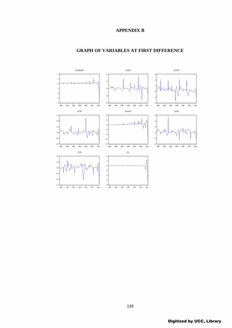
139

APPENDIX B

GRAPH OF VARIABLES AT FIRST DIFFERENCE

-.4

-.3

-.2

-.1

.0

.1

.2

1985 1990 1995 2000 2005 2010 2015

DLNRGDP

-.8

-.4

.0

.4

.8

1985 1990 1995 2000 2005 2010 2015

DLNIP

-.4

-.2

.0

.2

.4

.6

1985 1990 1995 2000 2005 2010 2015

DLNTP

-0.8

-0.4

0.0

0.4

0.8

1.2

1985 1990 1995 2000 2005 2010 2015

DCXP

-16

-12

-8

-4

0

4

8

1985 1990 1995 2000 2005 2010 2015

DLNCPI

-.4

-.2

.0

.2

.4

.6

1985 1990 1995 2000 2005 2010 2015

DLNK

-1.2

-0.8

-0.4

0.0

0.4

0.8

1985 1990 1995 2000 2005 2010 2015

DTR

-4

-3

-2

-1

0

1

2

1985 1990 1995 2000 2005 2010 2015

DL


growth impact of government consumption, … · university of cape coast . growth impact of...

Documents