Growth, Inequality and Poverty in Turkey with Emphasis

on Selected Countries in the Arab Region

Hasan Vergil (Istanbul University, Turkey)

Paper prepared for the IARIW-CAPMAS Special Conference “Experiences and Challenges in

Measuring Income, Wealth, Poverty and Inequality in the Middle East and North Africa”

Cairo, Egypt

November 23-25, 2015

Session 5: Inequality I

Tuesday, November 24, 2015

08:30-10:00

Paper Prepared for the IARIW-CAPMAS conference “Experiences and Challenges in Measuring Income, Wealth, Poverty and Inequality in

the Middle East and North Africa”

Cairo November 23-25, 2015

GROWTH, INEQUALITY AND POVERTY IN TURKEY WITH EMPHASIS ON SELECTED COUNTRIES IN THE ARAB REGION

Hasan Vergil

For additional information please contact:

Name: Hasan Vergil

Affiliation: İstanbul University, Turkey

Email Address: hasan.vergil@istanbul.edu.tr

GROWTH, INEQUALITY AND POVERTY IN TURKEY WITH EMPHASIS ON SELECTED COUNTRIES IN THE ARAB REGION

Abstract There exist little or no consensus on the relative effects of growth and distribution on poverty reduction. The present study examines the degree to which economic growth and income distribution affects poverty reduction, based on data starting 2005 for Turkey and available data for a sample of Arab countries. Estimations of panel data double log function, decomposition analyses and calculations of elasticity and pro-poor indices for Turkey show that, the poverty indices are more elastic to inequality changes than to changes in income in absolute terms. This suggests the important role of reducing inequality in reducing. It is also found that

the link between growth and changes in poverty indices are highly sensitive to the choice of poverty lines. Reducing inequality is important in order to reduce poverty in the selected Arab countries as in Turkey. Based on the pooled data, the results also suggest that growth rates of the selected Arab countries have generally been pro-poor with different degrees.

1. Introduction Although the intimate links between poverty, income distribution and the process of growth are largely discussed in the literature, so far, no consensus is reached about the ways inequality and economic growth matter for the reduction in poverty. Theoretical and empirical literature reveal that while economic growth can be bad for the poorest people in a country, through widening impact of economic growth on inequality, it can work more effectively to reduce poverty in the case of low inequality (Fields, 2001; Deininger and Squire, 1996; Dollar and Kraay, 2002, Kakwani and Son, 2006 and Nguyet and Hanh, 2012). Since the relationship between poverty, income distribution and economic growth largely depends on economic conditions of the countries such as the level of economic development and the initial level of inequality, individual country studies are needed to gain an appropriate understanding of this issue. The objective of this paper is thus to conduct a micro-level analysis of inequality and poverty changes to analyze the effect of the economic growth and the inequality on poverty in Turkey and assemble the findings with those found at World Bank’s POVCAL software for selected countries in the Arab region. Turkey has experienced a remarkable GDP growth rate of 5.06% in average between 2002 and 2013. However, Turkey also has the 3rd highest level of income inequality and the 3rd highest level of relative poverty in the OECD area. In addition, rural masses continues to migrate to urban areas in search of better livelihoods since 1950s which have resulted in considerable informal economy. All of these experiences of Turkey as a neighbor country to Arab World will shed light on understanding the nature of poverty and inequality and changes in both during the economic growth process in the Arab region which has per capita income level about one-half of the World and one-seventh of the OECD members as an average as of 2013. In spite of broadly maintained stability, the Arab countries have delivered relatively low economic growth needed for a substantial reduction in unemployment and poverty due mainly to unfavorable internal socio-political environment. Revealing the effects of economic growth and income distribution on poverty will carry great importance in shaping social policies in these countries. In addition, although poverty and inequality topics using Turkish data have been the subject of various studies before (e.g., Seker and Dayioglu, 2014 and TUSİAD,2014), the relationship among economic growth, inequality, and poverty reduction has not been elaborately quantified before.

In order to assess the relative importance of growth and inequality for reducing poverty, following analyses have been done for Turkey over the period 2005-2011; first, by splitting up Turkey into 12 different regions, an econometric model in the double log form for poverty has been estimated. Second, the overall growth elasticity of poverty and the overall Gini-inequality of poverty using the analytical approach by Kakwani (1993) and the parameterized approach by Bourguignon (2002) has been calculated. Third, the decomposition approach by Ravallion and Datt (1991) has been used to decompose the variation in FGT indices into growth and redistribution components. Fourth, pro-poor indices by Chen and Ravallion (2003), Kakwani and Pernia (2000) and Kakwani, Khandker and Son (2003) has been calculated. These indices also have been calculated for Algeria, Egypt, Jordan, Tunisia, Morocco and Yemen using pooled data found in World Bank’s POVCAL software. The results suggest that income redistribution and inequality reducing play an important role as the main contributor of the poverty reduction in Turkey and in selected Arab countries.

This paper is structured into five sections. The following section briefly reviews the literature on the relative roles of economic growth and inequality on poverty. The third section presents data and basic statistics. The fourth section presents methodology and empirical results and fifth section concludes.

2. Brief Literature Review

Eliminating absolute poverty is among the main focus of development goals. In reaching this goal, everybody is aimed to satisfy his/her basic needs which might change across countries and time. If a poverty line is raised to average income, both more people is portrayed as a poor and relative deprivation matters more. Achieving the goal of reducing both absolute and relative poverty requires understanding the links between poverty, growth and distribution and implementing country-specific, perfectly blending growth and distribution policies. Poverty, inequality and economic growth are closely linked with each other through influencing one another directly and indirectly. For example, growth influences poverty directly and it influences poverty indirectly, through influencing inequality. In this paper, we are only interested in this aspect of the relation; analyzing the effect of the economic growth and inequality on poverty. We have not dealt with the reciprocity between economic growth, inequality and poverty. The analysis of how reduction in poverty depends on changes in growth rate and/or inequality is displayed through calculations of some indicators such as the elasticity of poverty with respect to income and inequality, poverty decomposition and whether the growth experienced is pro-poor or not. Kakwani (1993), Epaulard (2003) and Bourguignon (2003) show that while growth elasticity of poverty is always negative, inequality elasticity of poverty is positive with a sufficient level of mean income. The theoretical expectations are also verified by all empirical studies. Different arguments have been put forth in the literature in order to assess the relative importance of economic growth and income distribution. Some studies argue that growth affect dominates in reducing poverty. For example; Dollar and Kraay (2002) concluded that poor benefits from economic growth as much as anyone else in the society and growth enhancing policies aiming to reduce poverty effectively should take this strategy at the center. Ravallion (2001) argues that the poor will gain from growth but changes in inequality

during the growth process lead to heterogeneity in gains, therefore changes in inequality during the growth process should not be omitted. These arguments bring up the topic of how poverty reduction is sensitive to distribution changes. For example, White and Anderson (2001) find a high sensitivity of income of the poor to small changes in distribution. Wodon (1999) confirms that rural growth reduces inequality-sensitive poverty measures more than urban growth simply because growth is more associated with inequality in urban than in rural areas. He also finds for Bangladesh that the gains from growth have not been as large as they would have been because of the rise in inequality. Similarly, if a country has a high inequality, growth might be less effective in reducing poverty (Mckay, 1997; Hanmer and Naschold2000). This argument is confirmed by Bruno, Ravallion and Squire (1998) who showed by using data of 17 countries that holding the dispersion of income is the same, higher income growth causes larger poverty reduction and holding the growth rate constant, as distribution becomes more dispersed, poverty reduces in smaller rates. According to Bourguignon (2004), income distribution is as important as the growth rate in reducing poverty. Income distribution and growth rate simultaneously affect poverty. However, their effects differ depending on initial conditions of countries. Kalwij and Verschoor (2008) find evidence supporting these arguments. They examine the role of the distribution of income in determining the responsiveness of poverty to income growth and changes in income inequality using panel data of 58 developing countries for the period 1980–1998. Their estimations of income elasticity of poverty differed across countries conditional on the initial distribution of income. They conclude that while differing income growth rates account for most of the regional diversity in poverty trends, the additional impact of differences across regions in rates of inequality change and income and inequality elasticities of poverty is almost always significant and far too large to be ignored. There is also some evidence that growth has a bigger effect on poverty in rural areas than in urban areas (Ali and Thorbecke, 2000). However, Fosu (2010) finds substantial elasticity rural-urban differences without any specific pattern in the responsiveness of poverty to income growth across countries in Africa.

The literature so far shows little consensus on the relative effects of growth and distribution on poverty reduction. As Fields (2000) reports, one should pay attention on the appropriate measurement of poverty line for resolving the debate on the relative roles of economic growth and inequality for poverty reduction.

3. Data and Basic Statistics 3.1 Data for Turkey

Data for following analyses are obtained from Turkstat (Turkish Statistical Institute) which conducts Income and Living Conditions Survey (SILC) within the scope of the studies compliance with European Union and surveys have been carried out regularly in every year since 2006. Questionnaire on Income and Living Conditions Survey is formed in order to obtain target variables requested by EUROSTAT to calculate indicators such as income, poverty and other living conditions. In these surveys, using panel survey methodology, households have been designed as the final sampling unit and monitored throughout 4

years. Survey applications have been carried out with face to face interview basis/technique and information is recorded to portable computers. In the panel survey applications, the rotational design is used. According to this methodology, one part of the household stays in the sample frame from one year to another, a new sample household is added to the frame. Specifically, while the 75% of the sampling size is left in the frame of the panel, 25% of the sampling size changes in each year. Thus, panel application starts with the selection of the basic sampling which represents target population and individuals are monitored throughout 4 years with the direction of the rules of monitoring. The sampling size covers the entire members of the households that live within the borders of the Republic of Turkey. However the population in the aged home, elderly house, prisons, military barracks, private hospitals, hotels and child care centers together with the immigrant population were excluded out of the scope. Since the survey is conducted each year, an annual total available household income declared by the head of household is used in analyses. Household net annual disposable income is calculated as the total of individual usable income of all members of the household (total of the income in cash or in kind such as salary-wage, daily wage, enterprises income, pension, widowed-orphan salary, old-age salary, unpaid grants, etc.), adding the total of yearly income for the household (such as real property income, unreturned benefits, incomes gained by household members less than age 15, etc.) and subtracting taxes paid during the reference period of income and regular transfers to other households or persons1. In these surveys, the reference period for income information is “the previous calendar year”. For instance, income information of the 2009 refers to the income obtained in 2008. Thus, household total income is deflated by previous year’s CPI and incomes are converted to real terms by CPI 2005=100 using the database of Central Bank of Turkey. Since the standard of living of households depends on both its income and composition and number of household members, it will not be correct to calculate the individual income as total income divided by number of household members. In order to consider these factors, the modified equivalence scale of OECD which assigns a value of 1 for the reference person of the household, 0.5 for household members aged 14 and over and 0.3 for household members less than aged 14 is used for family members. The methodology of dividing total of household income by equivalent household size allows making better comparisons of the households with different size and structure. Total of 25822 real equalized incomes per household are recorded for 2006, 2007, 2008 and 2009 years and total 29912 real incomes per household are recorded for 2010, 2011 and 2012 years2.

3.2 Basic Statistics

Average annual per capita income of Arab world is above the 4500 USD as of 2013. This level is around half of the world average and around one seventh of the OECD average for the last two decade. Table 1 shows some indicators for the countries with available data in the World Bank databases. Among them Yemen is the least GDP level and Turkey has the highest. Based on the 1990 levels, Tunisia has almost doubled its GDP levels in 24 years. Egypt and Morocco followed Tunisia. All the countries in the sample showed better performance in the first decade of the 2000 compared to previous decade. However, due to

1 The Turkstat code for total household annual disposable income used in this study is HG110.

2 Turkstat publishes the SILC data in CDs and data for 2009 year exists in both 2006-2009 wave and 2009-2012

wave. Since number of households and identification number of households for the year 2009 are different in the waves, the data in the first wave with a larger data is used for the year 2009.

political turmoil in Yemen, average GDP growth rate of Yemen dropped to substantial rates for the period 2011-2013. Table 1: GDP Levels and Growth Rates for Selected Years

GDP per capita (annual) Average GDP Per capita growth (annual %)

Years / periods 1990 1995 2000 2005 2010 2013

1991-2000

2001-2010

2011-2013

Algeria 2544.5 2306.8 2487.3 3038.7 3143.6 3244.0 -0.19 2.39 1.05 Egypt 879.2 956.9 1140.1 1249.5 1550.1 1567.0 2.64 3.13 0.36 Jordan 1766.9 1881.8 1926.5 2326.5 2818.1 2855.3 0.99 3.89 0.44

Morocco 1416.9 1405.8 1609.0 1948.2 2348.6 2530.8 1.47 3.87 2.53 Turkey 5013.0 5417.1 6119.3 7129.7 7833.6 8728.8 2.11 2.63 3.71 Tunisia 2033.4 2237.7 2758.5 3217.9 3847.6 3979.4 3.11 3.39 1.15 Yemen 666.5 705.8 778.1 831.9 878.1 742.2 1.57 1.22 -5.05 Source: Calculations are based on Worldbank WDI database. GDP per capita is in terms of constant 2005 US$.

Life expectancy at birth is 67 years old as an average in the Arab world slightly less than the world average for the period 1990-2013. Turkey’s life expectancy has grown almost double compared to that of Arab World as an average for the period 1990-2013 and Turkey has the longest life expectancy among the countries in the sample. Tunisia has negative life expectancy growth rates between 2011 and 2013 years. Infant mortality rates per 1000 live births is 29.6 for the Arab World and 33.6 for the World as an average in 2013. Tunisia has the least rate in 2013. Turkey and Jordan are ranked after Tunisia. In lowering mortality rates, Turkey has performed best among the countries by lowering more than 3 times since 1990. Egypt and Jordan are other two countries lowered their mortality rates. Primary school enrollment rates of Arab world is less than the world average. Tunisia has the highest rates followed by Morocco and Egypt. Their enrollment rates are higher than enrollment rates of OECD members and high income countries as an average. The Poverty and Equity Database of World Bank shows that inequality indicators are scattered over the years. There is no regular inequality indices for the countries in the sample and no average inequality index for the Arab World. Turkey’s Gini index is around 0.40. Most of the time, the selected countries in the sample have lower Gini values than Turkey. In all countries, income shared by highest 20% is above 40% and income share held by lowest 20% is less than 10% showing that there is a considerable income inequality in these countries. Yemen, Egypt and Morocco have very high poverty headcount ratios and poverty gaps at $2 a day. Turkey has highest rural-urban poverty headcount ratio at national poverty lines (% of rural-urban population) as of 2012. The ratio rises as time passes. This trend shows Turkey’s success in reducing poverty in urban centers.

4. Methodology and Empirical Results 4.1 Econometric Estimation

In order to investigate the effects of inequality and growth on poverty in Turkey, the first step is to estimate the relationship by using least squares methodology. By doing this, data from Level 1 classification of Turkey’s regions by Turkstat is used for the time period 2006-2013 which includes the latest available data.3,4 Figure 1 and Figure 2 show the individual relationships between income and poverty and inequality and poverty, respectively. The relationship is negative between income and poverty while it is positive between inequality and poverty as theoretically expected; as income increases poverty decreases and as inequality worsens poverty rate rises. In order to determine which variable is more important in affecting poverty, the relationship among them must be estimated.

1.8

2.0

2.2

2.4

2.6

2.8

3.0

7.4 7.6 7.8 8.0 8.2 8.4 8.6 8.8 9.0 9.2 9.4 9.6

ln median income

ln p

overt

y r

ate

Figure 1: Poverty Rate and Income

1.8

2.0

2.2

2.4

2.6

2.8

3.0

-1.16 -1.12 -1.08 -1.04 -1.00 -0.96 -0.92 -0.88 -0.84 -0.80

ln GINI

ln P

overt

y R

ate

Figure 2: Poverty Rate and Gini

Source: The author, using the Turkstat data.

One of the methodologies to assess the effects of changes in income and distribution on poverty in a particular country is to form double log model for poverty (Ravallion, 1997; Ravallion and Chen, 1997; Ncube et.al. 2013). Theoretical argument for the poverty equation is provided by Kakwani (1993, p.18) who decomposes proportionate poverty as due to changes in average income and income inequality:

)()( ,,G

dGd

P

dPG

where, P, μ, and G shows poverty measure, average income and Gini coefficient, respectively

and , , G, is growth and inequality elasticity of poverty, respectively. While the effect of

the mean income on poverty is denoted by the first term, the effect of Gini index on poverty is measured by the second term. Based on this, it can be written as;

itititiit giniincomepoverty )ln()ln()ln( 21 (1) where; Poverty is a poverty rate which is defined as the proportion of the poor within the total population. Income is the median income of the regions. Gini is the Gini coefficient by

3 Data and further information about data can be obtained from the website address:

http://www.tuik.gov.tr/PreTablo.do?alt_id=1013 4 The list of the regions are; TR1 Istanbul, TR2 West Marmara, TR3 Aegean, TR4 East Marmara, TR5 West

Anatolia, TR6 Mediterranean, TR7 Central West Anatolia, TR8 West Black Sea, TR9 East Black Sea, TRA North East Anatoli, TRB Central East Anatolia, TRC South East Anatolia.

household disposable incomes. The available data requires that the relationship can be estimated by forming panel data which combines a cross-section dimension with a time series dimension. There are four kinds of panel data estimators: the pooled OLS (POLS), the fixed effect (FE), the first difference (FD) and the random effects (RE) depending on the assumptions made about the intercept term. In the POLS estimator, the intercept term is treated constant across all cross-sectional units. In the FE estimator, the intercepts are allowed to vary between cross-section units. The RE estimator also allows the intercepts vary between cross-section units but the variation is randomly determined. The FD estimator eliminates the unobserved heterogeneity by differencing variables across time. The appropriate model is selected depending on the assumptions made. If the unobserved individual effects are correlated with the explanatory variables, the FE and FD estimators should be used. When the individual effects are uncorrelated with the explanatory variables The RE estimator is the most efficient estimator. The most common test for the presence of an unobserved effect is the Lagrange multiplier (LM) test due to Breusch and Pagan (1980) and the Hausman test for correlation between an unobserved effect and the explanatory variables devised by Hausman (1978)5. Table 1 shows the results of the equation 1. The LM test concludes that the unobserved effects vary across regions and the Hausman test result suggests that the random effects model is an appropriate estimator. The Wald Chi-square statistic and z values reveal that all the coefficients in the model are different from zero. We don’t reject the homoscedasticity of assumption in the residuals of random effects model by W0, W10 and W50 test results. There is no cross-sectional dependence and the residuals are normally distributed. However, we reject the null hypothesis that there is no serial correlation by S.ALM and JT.LM test results. The existence of first order serial correlations in the residuals is the only assumption which is not met. However, since serial correlation tests are applied to panels with long times series (over 20-30 years), this is not a problem in micro panels with very few years as in our case with 8 years. Table 1. Estimation Results of Double Log Model: Dependent Variable: ln(poverty)

Variables Coefficient Std. Error z p>│z│

ln(income) -0.148 0.052 -2.85 0.004

In(gini) 0.796 0.280 2.84 0.005

constant 4.600 0.455 10.12 0.000

Statistics

Number of Observations: 96, R2: 0.26 Wald-Chi-square: 23.58 (0.00)

Hausman: 0.76 (0.68) LM: 10.00 (0.00)

W0: 1.34 (0.21), W50: 0.74 (0.68), W10: 1.34 (0.21) S.ALM: 6.52 (0.01), JT.LM: 16.51 (0.00)

Friedman: 14.91 (0.18), Frees: 0.254 Jarqua-Bera: 3.94 (0.14)

Notes: Poverty line is formed by using 50% of equivalised individual median income. The numbers in parentheses denote probability values which is the lowest significance level at which a null hypothesis is rejected.

LM is the chi-square value with one degree of freedom to test the null hypothesis of the variance of the unobserved effect is equal to zero.

Hausman is a chi-square value with two degrees of freedom to test the null hypothesis that unobserved effects are uncorrelated with explanatory variables.

5 The details for these tests are not given because they have been standard procedures in any panel data model

selection. The reader can consult econometrics textbooks for further details.

W0 is a the test statistic by Levene( 1960) and W50 and W10 are test statistics by Brown and Forsythe (1974) to test the homoscedasticity assumption in the residuals of random effects model.

S.ALM is a test statistic distributed with chi-square value with one degree of freedom developed by Baltagi and Li (1995) to test whether autocorrelation coefficient is zero and JT.LM is a test statistic by Baltagi and Li (1991) to test whether variance of unobserved effects and autocorrelation coefficient are jointly zero.

Friedman is a test statistic by Friedman (1937) to check for cross-sectional independence with a null hypothesis of no cross-sectional effects. Frees is a test statistic by Frees (1995) to test for cross-sectional correlations. Critical values for Frees’ Q Distribution are 0.3169, 0.4325, 0.6605 for 10%, 5% and 1% significance levels, respectively.

The estimations reveal that changes in poverty can be related to two main sources: changes in mean income and changes in relative incomes. While 1% increase in Gini coefficient increases inequality by 0.796 %, 1% increase in the median income of the regions decreases poverty rate by 0.148%. This result suggests that changes in income distribution is more effective in reducing poverty than the growth in mean income. In other words, poverty is more responsive to income distribution than economic growth. Since it is difficult to achieve poverty reduction solely through income distribution without economic growth, this evidence for Turkey reveals that economic growth associated with progressive distributional changes reduces poverty more than growth which leaves the distribution unchanged. As Bourguignon (2004) emphasized, changing the distribution is probably more important for reducing poverty for middle-income and relatively inequitable countries like Turkey. Thus redistribution policies may be more effective in reducing poverty in Turkey.

4.2 Standard Estimations

Having determined the relationship econometrically, the next analysis starts with the discussion of methodologies used to estimate the relationship from different aspects; first, the elasticity relationship between poverty, income and inequality and then decomposition of poverty and pro-poor indices will be briefly explained. In these calculations, the common measures are the Gini coefficient for inequality and a class of Foster, Greer, Thorbecke (1984) indices to measure poverty. The most widely used measure of inequality is the Gini coefficient. It can be calculated by aggregating the deficit between population shares (p) and the Lorenz curve which is the cumulative percentage of total income held by any bottom p of the population, L(p):

1

0

1

0

))((1))((2 dppLpdppLpG

It is an average difference between cumulated population shares and cumulated income shares. This equation can be applied to calculate the Gini coefficient for a population with values yi, i=1 to n, that are indexed in the non-decreasing order (yi < yi+1);

)

)1(

21(1

1

1

n

i

i

n

i

i

y

yin

nn

G

where yi is the per capita income of the ith person and n is the number of individual in the population.

The Gini coefficient provides a measure of inequality comparable across different sectors of population as well as countries and satisfies four highly desirable properties: the anonymity, scale independence, population independence and transfer principle. However, the Gini coefficient has a disadvantage, inter alia, that it cannot be decomposed into inequality within and inequality between groups. Once a welfare is measured and poverty line is known, poverty can be measured by a class of poverty gap indices developed by Foster, Greer and Thorbecke (1984), which may be written as;

)()(0

ydyfz

yzP

z

Where α reflects the degree of inequality among the poor, z is the poverty line, z – y (which is 0 when y > z) is the poverty gap with y is the expenditure or income of the ith poor household (or individual). When the parameter α =0, P0 is simply the headcount index. When α =1 and α =2, the index reflects intensity and severity of poverty, respectively. These are decomposable poverty measures such that a contribution of a subgroup to overall poverty can be calculated by disaggregating poverty into population subgroups.

4.2.1. Calculation of the Elasticity of Poverty

The degree of poverty depends on average income and income inequality. Poverty declines with a rise in average income and increases as inequality increases. Thus, any poverty measure can be written as;

))(,( pLPP

where, is a mean income and L(p) is a Lorenz curve measuring the relative income distribution.

The influence of income and inequality changes on poverty can be calculated by decomposition of a poverty measure into a growth effect and distribution effect. The growth effect comes out due to a change in when L(p) remains constant. The distributional effect comes out only because of the

change in L(p) when remains constant.

Kakwani (1993) derived the poverty elasticity of growth based on this equation for Foster, Greer and Thorbecke class of poverty measures as;

P

PP

P

P

1

, . for 0 and

H

zzf )(, for 0

where, H is the headcount ratio. These elasticities are always negative and denote percentage changes in poverty in response to 1 percentage change in the mean income of the society holding the inequality of income constant. In order to measure the effect of inequality on poverty, one has to deal with the problem of changes in income distributions due to economic growth. Kakwani (1993) assumed that the entire Lorenz curve shifts proportionally over the whole range and he identified shift of the Lorenz curve as:

)()()(* pLppLpL

where, is the proportional change in the Gini coefficient. Using such transformation of the Lorenz curve, Kakwani (1993) proposed following inequality of elasticity for the Foster, Greer and Thorbecke poverty measures;

z

z

P

P

P

G

G

PG

)(.. 1

,

for 0 and

H

zfzG

)()(,

for 0 .

The effects of changes in income and inequality on poverty is also estimated by modelling the distribution of income. Epaulard (2003) and Bourguignon (2003) assume that incomes are lognormally distributed. Adopting the methodology by Bourguignon (2003), the headcount index can be formally written as:

)()Pr( ZFzyH ttt

where Ft(Z) is the income distribution function. Under the assumption that incomes are lognormally distributed, the headcount measure of poverty can be expressed as:

t

t

tt

zH

2

1)/log(

where (.) is the cumulative normal distribution function and t is the standard deviation of

the logarithm of income. The relationship between the standard deviation, the Gini coefficient, G, and the cumulative distribution function is given by

12

2

t

tG

As in the Kakwani (1993), if a change in the poverty is decomposed as the growth rate of the mean income and the change in income distribution, the income elasticity of poverty can be defined as (Kalvij and Verschoor (2007);

0

)2

1)/log((

)2

1)/log((

1.

t

t

t

t

t

t

tt

t

t

t

z

z

H

H

where and are cumulative distribution function and normal density function, respectively. The

elasticity is negative and positively correlated with t . In addition, given the poverty line (z), the

smaller the inequality ( ), the more growth reduces poverty and the higher the mean income ( )

the more growth reduces poverty (Epaulard, 2003). Similarly, the elasticity of poverty with respect to inequality is given by;

02

1)/log(

)2

1)/log((

)2

1)/log((

.

t

t

t

t

t

t

t

t

t

t

t

t

t z

z

z

H

H

This elasticity is positive as long as the mean income is high enough such that

)2

1exp( 2

tt z .

Computing these two elasticities require knowing the parameters of poverty line, mean income and standard deviation of log income.

4.2.2. Decomposition Poverty into a Growth Effect and Redistribution Effects

The decomposition is useful in identifying contributions of different factors for the evolution of overall poverty. The literature offers different methods to decompose poverty. Kolenikov and Shorrocks (2005) develop a procedure which decomposes variation in poverty into mean income per capita, inequality and price sources. Ravallion and Huppi (1991) offer techniques which allow changes in poverty into changes among population subgroups and growth and redistribution components. This paper will use the methodology developed by Datt and Ravallion (1991) who decomposed the variation of poverty into distribution-neutral growth component, a redistribution component and a residual (See, Inchauste etal., 2014). Given the fact that any poverty measure can be written as a function of mean income (μ), the associated Lorenz curve (L) and the poverty line (z):

),,( tttt zLPP .

When the poverty line is held constant over time, the overall variation in poverty from the first period (t=0) to second period (t=1) can be expressed as;

),(),( 0011 LPLPP

The decomposition procedures differ according to reference period. If the first period is chosen, the growth component is equal to;

),(),( 0001 LPLPP .

Similarly, The redistribution component;

),(),( 0010 LPLPPL

The variation in overall poverty can be rearranged as;

),(),(),(),( 00011011 LPLPLPLPPPP L

The last term in brackets is called a residual which comprises the difference between the growth component based on the second period Lorenz curve and the same component based on the first period Lorenz curve. In order to eliminate the residual, one can use the Shapley (1953) value6 or take the average of double decomposition which uses the first year as a reference point in the first and the second year as a reference point in the second decomposition. The Shapley value decomposes the variation in the poverty index as an average of the marginal contributions of growth component and redistribution component as follows:

),(),(),(),(2

100011011 LPLPLPLPS ,

),(),(),(),(2

100100111 LPLPLPLPSL , and

LSSP

where S and LS are the Shapley contribution of the growth component and the Shapley

contribution of the redistribution component to a change in poverty, respectively.

4.2.3 Pro-poor Indices

6 The Shapley value is a solution concept in determining the payoff of a player in a group formed a coalition in

cooperative games. See, Inchauste etal., (2014) for further discussion.

A distinction between absolute and relative approach is important in measuring pro-poor growth. While the relative approach compares changes in the income of the poor with changes in non-poor income, the absolute definition places emphasis on how economic growth increases absolute living standards of the poor people. The Chen and Ravallion (2003)’s measure of pro-poor growth is based on the Watts index. They have measured mean growth rate of the poor by the area under the growth incidence curve up to the headcount ratio. They proposed that pro-poor growth rate is given by the ordinary growth rate times the ratio of the actual change in poverty over time (using the Watts index) to the change in poverty due to distribution neutral economic growth (Ravallion, 2004). Formally, it is expressed as:

*

t

tt

p

tdW

dWg

where, p

tg is pro-poor growth rate in country p, at time t, t is the ordinary growth rate, tdW and

*

tdW is the actual change in the Watts index and the change in the Watts index that would have been

observed with the distribution neutral growth rate, respectively.

If 0 t

p

tg , the growth is pro-poor, otherwise it is anti-poor.

Kakwani and Pernia (2000) proposed another pro-poor measure by decomposing total poverty reduction into the impact of growth and the impact of redistribution. This decomposition is identified in elasticities as:

where, is total poverty elasticity of growth, is percentage change in poverty when the

mean income grows 1% and relative inequality does not change and is a pure inequality

effect as a percentage change. They measure pro-poor growth by the ratio of total poverty elasticity to the percentage change in poverty when mean income grows 1% under constant inequality:

When 1 , the growth is strongly pro-poor, i.e. the poor benefit from growth more

proportionally than the rich. If 10 , then the growth is still pro-poor but the poor

benefit less proportionally than rich and if 0 , then the growth is not pro-poor.

The last measure is proposed by Kakwani, Khandker and Son (2003). They define the “poverty equivalent growth rate (PEGR)” as the growth rate that would have resulted in the same level of poverty reduction as the present growth rate if income distribution had not changed during the growth process.

The PEGR denoted by * is given by:

)(*

where, is a pro-poor index defined in Kakwani and Pernia (2000) and is the actual rate of

growth of mean income. The growth is pro-poor if * , and if *0 , the growth is

still pro-poor but accompanied by an increasing inequality. 4.3 Empirical Results

The empirical results comprise two parts. In the first part, using the data from surveys by Turkstat, Turkey’s poverty and inequality status will be displayed and calculations of elasticity of poverty, decomposition of poverty into a growth effect and redistribution effects and pro-poor indices will be presented. In the second part, using the grouped data from the Povcal data bank, pro-poorness indices will be calculated and readily available elasticity estimations will be presented for Algeria, Egypt, Jordan, Morocco, Tunisia and Yemen.

4.3.1 Empirical Results for Turkey

The analyses were done using two survey spells. The first step covers 2005-2008 years and the second spell covers 2008-2011 years. While Turkey has shown an outstanding economic growth performance during the first spell, the second spell covers the years after the global financial crisis of the 2007-2008 financial crisis which brought about almost a recession in Turkey’s economy. The unemployment rates went up to 13% in 2009, the economy contracted in the first quarter of 2009 and private consumption and investments have been contracted. Thus, the results from the calculations are evaluated by splitting the terms since the fundamentals and links among the variables seem to change in this period. In the first step, using the data from surveys by Turkstat, the inequality and poverty status of Turkey must be displayed before doing further analyses. Table 1 shows Turkey’s Gini coefficients across years. They have been above 0.40. These values are higher than the values reported in the World Bank Poverty and Equity Database. They imply that inequality is in improper range and too high. Table 1: Turkey’s Gini Coefficients across Years

Years: 2006 2007 2008 2009 2010 2011 2012

Estimate: 0.44 0.42 0.41 0.41 0.42 0.41 0.40

Source: Author’s calculations. Reference period of incomes is the previous calendar year.

When poverty line is determined as the 50% or the 60% of the mean income, the Foster- Greer-Thorbecke poverty measures across years follow similar trends. The poverty rates first decrease then increase in 2009 and 2010 and decrease again. The headcount ratio is close to 0.30 when the poverty line is 50% of the mean income (Table 2) and it is above 0.35 when the poverty line is 60% of the mean income (Table 3).

Table 2: Turkey’s Foster-Greer-Thorbecke Poverty Rates across Years (50% of the Mean Income)

Years 2006 2007 2008 2009 2010 2011 2012

α=0 0.32 0.30 0.28 0.29 0.29 0.28 0.27

α=1 0.118 0.099 0.092 0.095 0.097 0.092 0.088

α=2 0.059 0.045 0.042 0.044 0.046 0.043 0.041

Pov. line 3471.35 3748.44 3643.56 3529.78 3835.13 3743.48 3771.1

Source: Author’s calculations. Reference period of incomes is the previous calendar year.

Table 3: Turkey’s Foster-Greer-Thorbecke Poverty Rates across Years (60% of the Mean Income)

Years 2006 2007 2008 2009 2010 2011 2012

α=0 0.41 0.39 0.38 0.37 0.38 0.37 0.36

α=1 0.160 0.139 0.132 0.134 0.137 0.131 0.127

α=2 0.084 0.068 0.063 0.065 0.068 0.064 0.061

Pov. line 4165.62 4498.13 4372.27 4235.74 4602.16 4492.18 4525.32

Source: Author’s calculations. Reference period of incomes is the previous calendar year.

The absolute poverty which declares minimum standards for basic living needs is the more serious issue. Figure 1 and Figure 2 show poverty headcount rates for different income levels for two different survey spells cover the years 2005 and 2008 and 2009-2011. For example, when the income level is ₺4000, it is around 0.3. Turkey’s headcount ratios were lower in 2006 and 2007 compared to 2005 and 2008. Turkey’s headcount ratios followed very close trends for 2009, 2010 and 2011.

Figure 1: FGT Curves for 2006-2009

Source: Author’s calculations based on the Turkstat data. Reference period of incomes is the previous calendar

year.

Figure 2: FGT Curves for 2010-2012.

0.2

.4.6

.8

FG

T(z

, a

lpha

= 0

)

0 2000 4000 6000 8000 10000

Poverty line (z)

2006 2007

2008 2009

FGT Curves (alpha=0)

0.2

.4.6

.8

FG

T(z

, a

lpha

= 0

)

0 2000 4000 6000 8000 10000

Poverty line (z)

2010 2011

2012

FGT Curves (alpha=0)

Source: Author’s calculations based on the Turkstat data. Reference period of incomes is the previous calendar year.

Table 4 shows the elasticity of poverty rates with respect to income growth across years

using Kakwani (1993) and Bourguignon (2002) approaches when the poverty line is measured as the income level less than 50 % of the mean income. The two approaches provide similar results. As income grows 1%, as an average, the poverty headcount rate declines 1.60%. The elasticities of poverty gap and square of poverty gap are above the elasticity for the headcount ratio. The elasticity rate for the poverty gap square which attach greater weight to the poorest people is higher than the elasticity for the poverty gap. The elasticity ratios remain steady over the years.

Table 4: Elasticity of total poverty with respect to average income growth (Relative)

Headcount ratio Poverty Gap Poverty Gap Square

Years Kakwani (1993)

Bourguignon (2002)

Kakwani (1993)

Bourguignon (2002) Kakwani (1993)

2006 -1.67 -1.62 -2.29 -2.35 -2.8 2007 -1.46 -1.48 -1.9 -1.93 -2.15 2008 -1.57 -1.55 -1.93 -1.97 -2.14 2009 -1.56 -1.63 -2.05 -2.11 -2.36 2010 -1.61 -1.61 -2.02 -2.11 -2.32 2011 -1.72 -1.68 -2.06 -2.17 -2.32 2012 -1.65 -1.66 -2.01 -2.1 -2.23 Note: Poverty line is 50% of the mean income of each year. Reference period of incomes is the

previous calendar year.

Same elasticity calculations are shown in Table 5 with the poverty calculations based on daily $4.3 poverty line. The elasticity ratios are close to -3% for the headcount ratio and above -3% for the measures of poverty gap and poverty gap square measures as an average. The elasticity rate for the poverty gap square which attach greater weight to the poorest people is higher than the elasticity rate for the poverty gap. It means that the impact of income growth on the severely poor is greater than its impact on moderately poor. The elasticity rates calculated by Bourguignon approach are higher than the elasticity rates calculated by Kakwani approach. The elasticity rates remain steady over the years.

Table 5:Elasticity of total poverty with respect to average income growth (Absolute)

Headcount ratio Poverty Gap Poverty Gap Square

Years Kakwani (1993)

Bourguignon (2002)

Kakwani (1993)

Bourguignon (2002) Kakwani (1993)

2006 -4.17 -4.54 -5.98 -5.62 -6.08 2007 -2.55 -2.69 -2.61 -3.01 -2.54 2008 -2.56 -2.7 -2.64 -2.87 -2.45 2009 -2.75 -2.95 -3.02 -3.26 -2.95 2010 -3.18 -3.12 -3.37 -3.53 -3.12 2011 -2.79 -2.99 -3.21 -3.28 -3.27 2012 -2.63 -2.82 -2.78 -2.99 -2.72

Notes: Poverty line is $4.3. Equivalence of $1 to Turkish Lira with respect to purchasing power parity for each year is obtained from Turkstat. Reference period of incomes is the previous calendar year.

Table 6 shows elasticity of total poverty with respect to inequality with two different

Table 7 decomposes the change in Turkey's poverty rates between 2005 and 2008 in terms of the effect of growth and of changes in inequality. Poverty reduction is higher if it is measured by the headcount ratio whether poverty is absolute or relative. Of the 3.1 percentage change in the reduction of the poverty headcount ratio can be attributed into improvements in the income distribution as 3.2 percentage point. Although it is negligible, the pure economic growth effects (average growth rate was 6% during this period) have partly offset this poverty reduction. Thus it can be concluded that in the period 2005-2008, income redistribution is the main contributor of the poverty reduction. Table 7: Growth and Inequality Components of FGT Poverty Measures (2006-2009)

Absolute Poverty P1 P2 Poverty Reduction

Growth Component

Redistribution Component

α=0 0.0647 0.0334 -0.0313 0.0009 -0.0322

α=1 0.0176 0.0085 -0.0091 0.0002 -0.0093

α=2 0.0069 0.0036 -0.0033 0.0001 -0.0034

Relative Poverty P1 P2 Poverty Reduction

Growth Component

Redistribution Component

α=0 0.3443 0.3193 -0.025 0.0023 -0.0273

α=1 0.1252 0.1036 -0.0216 0.0014 -0.023

α=2 0.0636 0.0471 -0.0165 0.0008 -0.0173

Notes: Growth and redistribution components are calculated by Shapley approach. For absolute poverty, the

poverty line is calculated as the income of the average of the period based on daily $4.3. For relative poverty,

the poverty line is 50% of the mean income of the average of the period. Reference period of incomes is the

previous calendar year.

poverty levels. They have theoretically expected signs. The elasticity rates do not show systematic changes over time. The rates are highest for the measure of poverty gap square which attach greater weight to poorest persons. The elasticity rates calculated by absolute poverty measures unusually high for some years. It should be noted that the poverty indexes are more elastic to inequality changes than to changes in income in absolute terms. This suggests the important role of reducing inequality in reducing poverty which is in conformity with the econometric result above. Table 6: Elasticity of total poverty with respect to inequality (relative and absolute)

Years Headcount ratio Poverty gap Poverty gap square

relative absolute relative absolute relative absolute

2006 1.67 18.07 4.9 36.46 8.52 46.55

2007 1.46 10.67 3.78 15.19 5.81 18.77

2008 1.57 10.27 3.78 14.61 5.76 17.74

2009 1.56 9.86 4.08 15.39 6.42 20.03

2010 1.99 13.79 4.73 19.7 7.36 22.55

2011 1.61 10.66 3.92 17.46 6.18 22.86

2012 1.68 9.95 3.99 17.17 6.12 19.67

Notes: Elasticities are calculated by the methodology of Kakwani (1993). Poverty line is 50% of the mean income of each year in the relative approach. Reference period of incomes is the previous calendar year. Poverty line is $4.3 in the absolute approach. Equivalence of $1 to Turkish Lira with respect to purchasing power parity for each year is obtained from Turkstat.

Tables 8 shows the decomposition of poverty reduction between 2009 and 2011 into income growth and redistribution components for different poverty measures. In this period, the largest poverty reduction is observed in the headcount ratio. Of the 0.72% absolute poverty reduction, while 0.07% poverty reduction is attributed to the income growth, 0.65 % of that is attributed to redistribution of income. Similarly, of the 1.99% relative poverty reduction, while the income growth has a share of 0.27%, redistribution component contributes poverty reduction 1.72%. Again, it can be concluded that in the period 2009-2011, an income redistribution is the main contributor of the poverty reduction. Economic growth has contributed very little to the poverty change. Table 8: Growth and Inequality Components of FGT Poverty Measures (2010-2012)

Absolute Poverty P1 P2 Poverty Reduction

Growth Component

Redistribution Component

α=0 0.0383 0.0311 -0.0072 -0.0007 -0.0065

α=1 0.0086 0.0077 -0.0009 -0.0002 -0.0007

α=2 0.0031 0.0033 0.0002 -0.0001 0.00029

Relative Poverty P1 P2

Poverty Reduction

Growth Component

Redistribution Component

α=0 0.2813 0.2614 -0.0199 -0.0027 -0.0172

α=1 0.0949 0.0844 -0.0105 -0.0012 -0.0093

α=2 0.0446 0.0388 -0.0057 -0.0006 -0.0051

Notes: Growth and redistribution components are calculated by Shapley approach. For absolute poverty, the poverty line is calculated as the income of the average of the period based on daily $4.3. For relative poverty, the poverty line is 50% of the mean income of the average of the period. Reference period of incomes is the

previous calendar year. In order to calculate pro-poor growth rates, data is balanced, i.e., incomes of the same individuals are observed over the period. The methodologies proposed by Ravallion and Chen (2003), Kakwani and Pernia (2000) and Kakwani, Khandker and Son (2003) are used to calculate pro-poor indices for Turkey’s growth rates. Table 9 shows results of pro-poor indices for the period between 2005 and 2008. Turkey’s growth rates were pro-poor according to Ravallion and Chen (2003) and Kakwani, Khandker and Son (2003) indices and strongly pro-poor according to Kakwani and Pernia (2000) index for all poverty measures and poverty lines. The pro-poor index for the poverty gap and squared gap measures tends to be lower than the pro-poor index of the poverty rate in Kakwani and Pernia (2000) and and Kakwani, Khandker and Son (2003) indices for absolute poverty line. It implies that the poorest benefited proportionally less than the poor who were closer to the poverty line. However, when the relative poverty line is measured the reverse is true. The poorest benefited proportionally more than the poor who were closer to the poverty line. Thus, the link between growth and changes in poverty indices are highly sensitive to the choice of poverty lines. The variability of the impact of growth on poor depends on the relative position of the person among the poor determined by the poverty line.

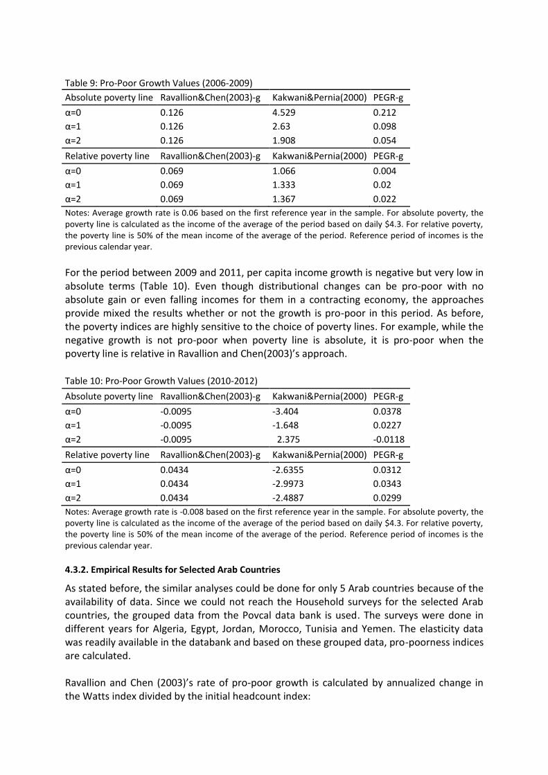
Table 9: Pro-Poor Growth Values (2006-2009)

Absolute poverty line Ravallion&Chen(2003)-g Kakwani&Pernia(2000) PEGR-g

α=0 0.126 4.529 0.212

α=1 0.126 2.63 0.098

α=2 0.126 1.908 0.054

Relative poverty line Ravallion&Chen(2003)-g Kakwani&Pernia(2000) PEGR-g

α=0 0.069 1.066 0.004

α=1 0.069 1.333 0.02

α=2 0.069 1.367 0.022

Notes: Average growth rate is 0.06 based on the first reference year in the sample. For absolute poverty, the poverty line is calculated as the income of the average of the period based on daily $4.3. For relative poverty, the poverty line is 50% of the mean income of the average of the period. Reference period of incomes is the previous calendar year.

For the period between 2009 and 2011, per capita income growth is negative but very low in absolute terms (Table 10). Even though distributional changes can be pro-poor with no absolute gain or even falling incomes for them in a contracting economy, the approaches provide mixed the results whether or not the growth is pro-poor in this period. As before, the poverty indices are highly sensitive to the choice of poverty lines. For example, while the negative growth is not pro-poor when poverty line is absolute, it is pro-poor when the poverty line is relative in Ravallion and Chen(2003)’s approach. Table 10: Pro-Poor Growth Values (2010-2012)

Absolute poverty line Ravallion&Chen(2003)-g Kakwani&Pernia(2000) PEGR-g

α=0 -0.0095 -3.404 0.0378

α=1 -0.0095 -1.648 0.0227

α=2 -0.0095 2.375 -0.0118

Relative poverty line Ravallion&Chen(2003)-g Kakwani&Pernia(2000) PEGR-g

α=0 0.0434 -2.6355 0.0312

α=1 0.0434 -2.9973 0.0343

α=2 0.0434 -2.4887 0.0299

Notes: Average growth rate is -0.008 based on the first reference year in the sample. For absolute poverty, the poverty line is calculated as the income of the average of the period based on daily $4.3. For relative poverty, the poverty line is 50% of the mean income of the average of the period. Reference period of incomes is the previous calendar year.

4.3.2. Empirical Results for Selected Arab Countries

As stated before, the similar analyses could be done for only 5 Arab countries because of the availability of data. Since we could not reach the Household surveys for the selected Arab countries, the grouped data from the Povcal data bank is used. The surveys were done in different years for Algeria, Egypt, Jordan, Morocco, Tunisia and Yemen. The elasticity data was readily available in the databank and based on these grouped data, pro-poorness indices are calculated. Ravallion and Chen (2003)’s rate of pro-poor growth is calculated by annualized change in the Watts index divided by the initial headcount index:

)(

)()(

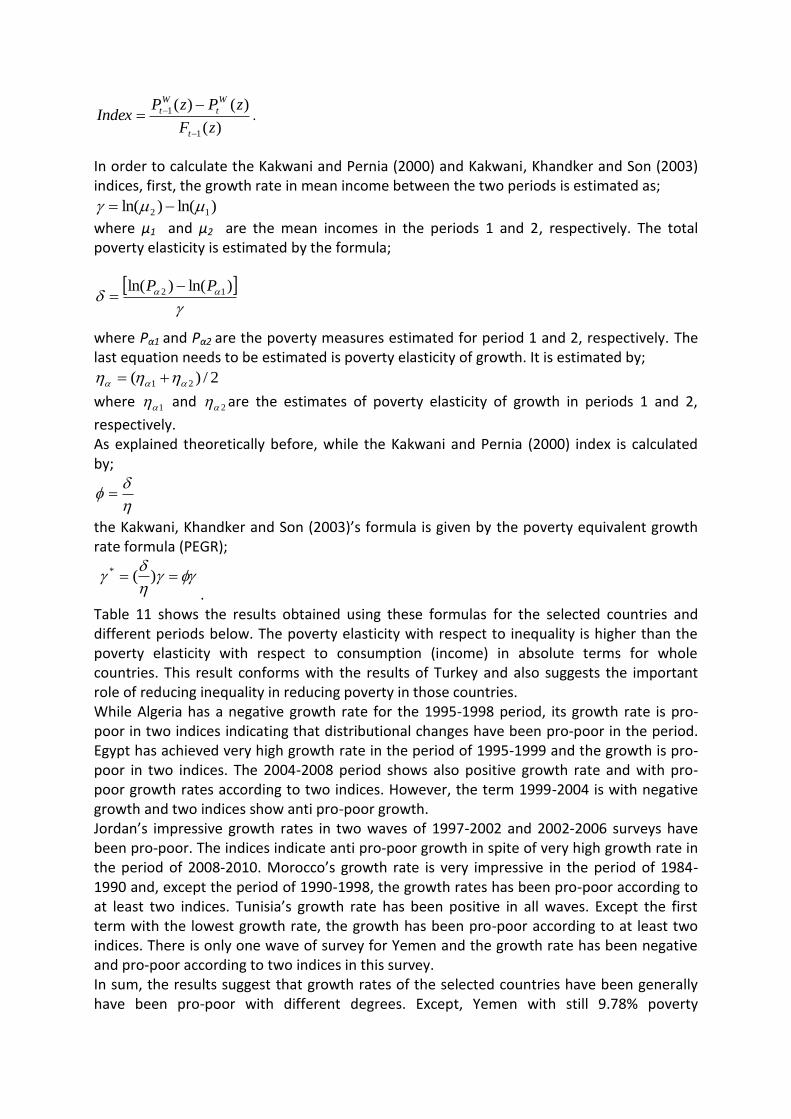
1

1

zF

zPzPIndex

t

W

t

W

t

.

In order to calculate the Kakwani and Pernia (2000) and Kakwani, Khandker and Son (2003) indices, first, the growth rate in mean income between the two periods is estimated as;

)ln()ln( 12 where μ1 and μ2 are the mean incomes in the periods 1 and 2, respectively. The total poverty elasticity is estimated by the formula;

)ln()ln( 12 PP

where Pα1 and Pα2 are the poverty measures estimated for period 1 and 2, respectively. The last equation needs to be estimated is poverty elasticity of growth. It is estimated by;

2/)( 21

where 1 and 2 are the estimates of poverty elasticity of growth in periods 1 and 2,

respectively. As explained theoretically before, while the Kakwani and Pernia (2000) index is calculated by;

the Kakwani, Khandker and Son (2003)’s formula is given by the poverty equivalent growth rate formula (PEGR);

)(*

. Table 11 shows the results obtained using these formulas for the selected countries and different periods below. The poverty elasticity with respect to inequality is higher than the poverty elasticity with respect to consumption (income) in absolute terms for whole countries. This result conforms with the results of Turkey and also suggests the important role of reducing inequality in reducing poverty in those countries. While Algeria has a negative growth rate for the 1995-1998 period, its growth rate is pro-poor in two indices indicating that distributional changes have been pro-poor in the period. Egypt has achieved very high growth rate in the period of 1995-1999 and the growth is pro-poor in two indices. The 2004-2008 period shows also positive growth rate and with pro-poor growth rates according to two indices. However, the term 1999-2004 is with negative growth and two indices show anti pro-poor growth. Jordan’s impressive growth rates in two waves of 1997-2002 and 2002-2006 surveys have been pro-poor. The indices indicate anti pro-poor growth in spite of very high growth rate in the period of 2008-2010. Morocco’s growth rate is very impressive in the period of 1984-1990 and, except the period of 1990-1998, the growth rates has been pro-poor according to at least two indices. Tunisia’s growth rate has been positive in all waves. Except the first term with the lowest growth rate, the growth has been pro-poor according to at least two indices. There is only one wave of survey for Yemen and the growth rate has been negative and pro-poor according to two indices in this survey. In sum, the results suggest that growth rates of the selected countries have been generally have been pro-poor with different degrees. Except, Yemen with still 9.78% poverty

headcount rates in 2005, it can be said that countries in the sample have been successful in reducing their headcount poverty rates in the periods investigated. Even though we have an extreme example of Jordan in which all indices indicate anti pro-poor growth in spite of very high growth rate in the period of 2008-2010, the relationship between growth and reducing poverty seems to be positive.

Table 11: Total Poverty Elasticity and Pro-poor Growth Indices for Selected Countries Periods Elasticity

with respect to consumption

Elasticity with respect to Gini

Periods Ravallion and Chen(2003)-g

Kakwani and Pernia(2000)

PEGR-g Growth rate

Algeria

1995 -3.5400 8.4138 1995-1998 0.0085* -0.6267 0.0788* -0.048

1998 -3.5387 7.8460

Egypt

1990 -5.9015 9.7654 1990-1995 0.0903* -3.0770 0.1248* -0.031

1995 -6.7719 10.6640 1995-1999 -0.1218 0.3586* -0.0878Ψ 0.137

1999 -5.6612 11.0527 1999-2004 -0.0363 1.9206** -0.0196 -0.021

2004 -5.1610 9.7557 2004-2008 -0.0146 1.6234** 0.0233* 0.037

2008 -4.6300 9.2624

Jordan

1992 -4.5893 16.5071 1992-1997 0.2415* -0.9471 0.2700* -0.139

1997 -4.6521 13.9639 1997-2002 -0.0295 0.3154* -0.098 Ψ 0.143

2002 -6.4888 23.4834 2002-2006 0.0094* 2.8730** 0.1839* 0.098

2006 -4.3547 17.8347 2006-2008 0.2238* -10.7602 0.2784* -0.024

2008 -5.8604 23.3026 2008-2010 -0.2027 -0.1807 -0.1478 0.125

2010 -4.5332 21.0326

Morocco

1984 -2.6277 5.1792 1984-1990 -0.1011 1.0744** 0.0238* 0.320

1990 -5.7202 17.6768 1990-1998 -0.1917 1.1727** -0.0311 -0.180

1998 -3.8598 9.3224 1998-2000 0.0068* 0.6346* -0.011 Ψ 0.029

2000 -4.3149 10.8543 2000-2007 -0.1108 1.1481** 0.0271* 0.183

2007 -4.1774 13.4594

Tunisia

1990 -3.0735 9.1666 1990-1995 0.0027* -1.7082 -0.0503 0.019

1995 -3.1883 9.7468 1995-2000 -0.0086 1.4541** 0.0764* 0.168

2000 -4.4396 16.8715 2000-2005 -0.0164 1.5835** 0.0543* 0.093

2005 -3.8556 16.4563 2005-2010 -0.0145 1.2664** 0.0347* 0.130

2010 -3.6594 18.3008

Yemen

1998 -3.0328 4.7064 1998-2005 0.0756* -0.6261 0.0516* -0.032

2005 -3.8971 5.7369

Notes: The data is obtained from PovcalNet. The $1.25 a day global poverty line is used as a poverty

line. The mean income is the average monthly per capita income/consumption expenditure from the

surveys in 2005 PPP. The poverty measure is the headcount poverty rates. “*”, “**” and “Ψ” shows

that the growth is pro-poor, strongly pro-poor and pro-poor but with increasing inequality in the

period considered.

Theoretically, we expect a positive relationship between the level of development and growth and inequality elasticity of poverty and the reverse relationship between the inequality level and growth and inequality elasticity, respectively (Bourguignon, 2004). Assuming that constant per capita income levels indicate development levels and Gini coefficients indicate inequality levels, we find weak evidence for this expectation. Average cross-section data show that Yemen has a lowest per capita income among the countries and has a lowest consumption (income) elasticity and Gini elasticity of poverty, respectively. This is in conformance with the expectations. However, while Algeria has a highest per capita income, it has a second lowest rankings in terms of consumption (income) elasticity and Gini elasticity of poverty, respectively. Egypt has a lowest Gini coefficient and highest consumption elasticity of poverty as theoretically expected. Since inequality levels and growth rates of countries change over time, poverty reduction in these countries changes depending on relative changes in income and distribution. Unfortunately lack of data in the countries does not allow us to discuss this argument elaborately by providing more evidence.

5. Conclusion This study aims to investigate the degree to which economic growth and income distribution

affects poverty reduction for Turkey and for a sample of Arab countries. The analyses for Turkey were done using two survey spells; 2006-2009 and 2009-2012. The fundamentals and links among the variables seem to change in the second spell due mainly to economic crisis in the USA in 2008. The surveys were done in different years for Algeria, Egypt, Jordan, Morocco, Tunisia and Yemen. The income elasticity of poverty headcount ratio is around -1.60% when the relative poverty line is used and close to -3% when the absolute poverty line is used over the whole period. The elasticities of poverty gap and square of poverty gap are above the elasticity for the headcount

ratio. The income elasticity rate for the poverty gap square which attach greater weight to the poorest people is higher than the income elasticity for the poverty gap. The inequality elasticity of poverty is highest for the measure of poverty gap square which attach greater weight to poorest

persons. The poverty indexes are more elastic to inequality changes than to changes in income in absolute terms. This suggests the important role of reducing inequality in reducing poverty which is in conformity with the econometric results.

The decomposition of poverty reduction reveals that an income redistribution is the main contributor of the poverty reduction in both spells. The poverty reduction was higher in the first spell despite offsetting effects of the pure economic growth to the poverty reduction. In the second spell, both income growth and income redistribution have contributed to poverty reduction. In the whole period, economic growth has contributed very little to the poverty change. In the first wave of the survey which includes the period 2005-2008, the pro-poor indices reveal that Turkey’s growth rates were pro-poor according to Ravallion and Chen (2003) and Kakwani, Khandker and Son (2003) indices and strongly pro-poor according to Kakwani and Pernia (2000) index for all poverty measures and poverty lines. The choice of poverty lines strongly

determines the results as the results are reversed for the poorest groups in this period. The pro-poorness is inconclusive in the second wave which includes 2009-2011 period as the indices provide mixed results.

The analyses for selected Arab countries provide similar results; the poverty elasticity with respect to inequality is higher than the poverty elasticity with respect to consumption (income) in absolute terms suggesting the important role of reducing inequality in reducing poverty in those countries. The results suggest that growth rates of the selected countries have been generally have been pro-poor with different degrees. Except, Yemen with still 9.78% headcount rates in 2005, it can be said that countries in the sample have been successful in reducing their headcount poverty rates in the periods investigated. References:

Ali, A. and Thorbecke, E. (2000). “The State and Path of Poverty in sub-Saharan Africa: Some Preliminary Results”, Journal of African Economies, 9, 9-40. Baltagi, B. H and Li Q., (1991). “A Joint Test for Serial Correlation and Random İndividuals Effects”, Statistics and Probability Letters, 11, 277-280. Baltagi, B. H and Li Q., (1995). “Testing AR(1) and Against MA(1) Disturbances in an Error Component Model”, Journal of Econometrics, 68, 133-151. Bourguignon, Francois (2004). ‘The Poverty-Growth-Inequality Triangle’. Paper presented at the Indian Council for Research on International Economic Relations, New Delhi, February 4. Breusch, T. S. and A.R. Pagan (1980). "The Lagrange Multiplier Test and Its Applications to Model Specification in Econometrics," Review of Economic Studies, 47(1), 239-253. Brown, Mortan B. and Alan B. Forsythe (1974). “Robust Tests for the Equality of Variances”, Journal of the American Statistical Association, Vol. 69, No. 346 (Jun., 1974), pp. 364-367. Datt, Gaurav, and Martin Ravallion. (1991). “Growth and Redistribution Components of Changes in Poverty Measures: A Decomposition with Applications to Brazil and India in the 1980s.” Living Standards Measurement Study Working Paper No. 83, World Bank, Washington, DC. Deininger, Klaus and Lyn Squire (1996). “A New Data Set Measuring Income Inequality”, The World Bank Economic Review, Volume: 10, Number:3, 565-591. Dollar, David and Aart Kraay (2002). “Growth is Good for the Poor”, Journal of Economic Growth, 7, 195-225. Fosu, A. K. (2010). “Income Distribution and Growth’s Ability to Reduce Poverty: Evidence from Rural and Urban African Economies”, UNU-WIDER, Working Paper No. 2010/92. Frees, E. W. (1995). “Assessing Cross-Sectional Correlations in Panel Data”, Journal of Econometrics, 69, 393-414.

Friedman, M. (1937). “The Use of Ranks to Avoid the Assumption of Normality Implicit in the Analysis of Variance”, Journal of the American Statistical Association, 32, 675-701. Fields, Gary S. (2001). Distribution and Development: a new Look at the Developing World, The MIT Press, Cambridge, Massachusetts. Fields, G.s. (2000). “The Dynamics of Poverty, Inequality, and Economic Well-being: African Economic Growth in Comparative Perspective”, Journal of African Economies, 9 (suppl. 1): 45-78. Hanmer, L. and Naschold, F. (2000). “Attaining the International Development Targets: Will Growth be Enough?”, Development Policy Review, 18, 11- 36. Hausman, J. A. (1978). Specification tests in econometrics. Econometrica, 46(6):1251– 1272. Inchauste, Gabriela, João Pedro Azevedo, B. Essama-Nssah, Sergio Olivieri, Trang Van Nguyen, Jaime Saavedra-Chanduvi and Hernan Winkler. (2014). Understanding Changes in Poverty, The World Bank, Washington DC. Kakwani, N. (1993). "Poverty and Economic Growth with Application to Côte D’Ivoire", Review of Income and Wealth, 39(2): 121:139. Kakwani, N., S. Khandker, and H. Son (2003): “Poverty Equivalent Growth Rate: With Applications to Korea and Thailand,” Tech. rep., Economic Commission for Africa. Kakwani, Nanak and Hyun H. Son (2006). “Global Estimates of Pro-Poor Growth”, International Poverty Center Working Paper, Number: 31. Kakwani, N. and Pernia, E. (2000) “What is Pro-poor Growth”, Asian Development Review, Vol. 16, No.1, 1-22. Kolenikov, Stanislav, and Anthony Shorrocks. 2005. “A Decomposition Analysis of Regional Poverty in Russia.” Review of Development Economics 9 (1): 25–46. Levene, H. (1960). “Robust Tests for Equality of Variances”, In Contributions to Probability and Statistics (I. Olkin, ed.) 278–292. Stanford Univ. Press, Palo Alto, CA. McKay, A. (1997). “Poverty Reduction through Economic Growth: Some Issues”, Journal of International Development, 9, 665-673. Ncube, M.; Anyanwu, J.C. and Hausken, K. (2013), Inequality, Economic Growth, and Poverty in the Middle East and North Africa (MENA), Working Paper Series N° 195 African Development Bank, Tunis, Tunisia.

Nguyet, Pham Minh and Nguyen Thi Hong Hanh (2012). “Growth, Inequality and Poverty in Vietnam, 1993-2008”, EADN Working Paper, Number: 62. Ravallion, M. (1997), “Can high-inequality developing countries escape absolute poverty?”, Economic Letters, September 56(1), pp.51-57. Ravallion, Martin, 2001. “Growth, Inequality and Poverty: Looking Beyond Averages”, World Development, Vol.29, No:11, pp. 1803-1815. Ravallion, Martin, 2004. "Pro-poor growth: A primer," Policy Research Working Paper Series 3242, The World Bank. Ravallion, M. and Chen, S. (1997), “What can new survey data tell us about recent changes in distribution and poverty?”, World Bank Economic Review, 11(2), 357–382. Ravallion, M. and Chen, S. (2003) “Measuring Pro-poor Growth”, Economic Letters, Vol. 78 (1), 93-99 Ravallion, Martin, and Monika Huppi. 1991. “Measuring Changes in Poverty: A Methodological Case Study of Indonesia during an Adjustment Period.” World Bank Economic Review 5 (5): 57–82. Seker, Sirma Demir and Meltem Dayioglu (2014). “Poverty Dynamics in Turkey”, Review of İncome and Wealth, DOI: 10.1111/roiw.12112. SHAPLEY, L. (1953). "A value for n-person games," in Contributions to the Theory of Games, ed. by H. W. Kuhn and A. W. Tucker, Princeton: Princeton University Press, vol. 2 of Annals of Mathematics Studies, 303-317. TUSİAD (2014). “Türkiye’de Bireysel Gelir Dağılımı Eşitsizlikleri: Fonksiyonel Gelir Kaynakları ve Bölgesel Eşitsizlikler (Personel Income Distribution Inequalities in Turkey: Functional Income Resources and Regional Inequalities)”, No: TUSİAD-T/2014-06/554. White, H. and Anderson, E. (2001), “Growth versus Distribution: Does the Pattern of Growth Matter?”, Development Policy Review, 19, 267-289. Wodon, Q. (1999). Growth, Poverty and Inequality: A Regional Panel for Bangladesh. Washington, D.C.: World Bank.