growth of skipjack
TRANSCRIPT

2 7 MAI 1980
Occasional Paper No.11
GROWTH OF SKIPJACK
E. J o s s e , J . C . Le Guen, R. K e a r n e y , A. Lewi s , A. S m i t h , L. Marec e t
P .K. Tomlinson
SPC Library
35919 Bibliotheque CPS
South Pacific Commission Noumea, New Caledonia
522/80 January 19 79
LIBRARY SOUTH PA Cfn.r COMMISSION

Occasional Paper No. 11
GROWTH OF SKIPJACK (Katsuwonus pelamis)
E. Josse, J.C. Le Guen ORSTOM - Noumea, New Caledonia
*
R.E. Kearney,* A.D. Leswis,** B.R. Smith Fisheries Division
Ministry of Primary Industry Konedobu, Papua New Guinea
*
L. Marec ORSTOM - Papeete, Tahiti
and
P.K. Tomlinson IATTC - La Jolla, California
*New address: South Pacific Commission, Noumea, New Caledonia
**New address: Australian National University, Research School of Biological Sciences, Canberra, Australia
South Pacific Commission Noumea, New Caledonia
January 1979
sc«;Th >;A; ;f,c COMMISSION

CONTENTS
Page
INTRODUCTION
I. Age reading from hard part structures 1
A. Seasonal marks (vertebrae, scales, dorsal spines) 1
B. General remarks on the interpretation of 3
seasonal marks in tropical environments for growth studies
C. Daily growth marks on the otoliths 4
D. Conclusions 4
I I . Growth observed from tagging studies 5
I I I . Petersen 's method 2 1
A. General considerations 21
B. Representativeness of the samples
CONCLUSIONS
ACKNOWLEDGEMENTS
REFERENCES
24
77 IV. Formulation of the growth results
A. General remarks on von Bertalanffy's model 27
B. Mathematical formulation of growth 30
rates obtained from tagging studies
32
34
35
ANNEX I - Tagging of Skipjack Tuna 4 1
ANNEX II - Sampling of Skipjack Tuna 6 5
FIGURES 78

GROWTH OF SKIPJACK ( Katsuwonus pelamis)
INTRODUCTION
For more than twenty years fishery biologists have assiduously investigated the problem of growth in skipjack tuna, particularly in the Pacific. The. various teams of tuna specialists, national and international, have furnished more or less exhaustive accounts of the numerous studies undertaken and results published on growth. Nowhere have we found an examination in depth of these results, an examination which has now become necessary with the reawakening of interest in the biological and ecological parameters in the models of production. The variety of growth rates estimated for skipjack, ranging from simple to double, or even triple, certainly poses a problem of choice for students of population dynamics.
We therefore propose to review the principal types of work enabling estimation of growth, at the same time analyzing in detail the various hypotheses, implicit or explicit, which the authors have made, as well as the comparability of the requisite basic data.
I. AGE READING FROM HARD PART STRUCTURES (vertebrae, scales, dorsal spines, otoliths)
A. Seasonal marks (vertebrae, scales, dorsal spines)
Reading the vertebrae to estimate age in skipjack has been practised since the 1930s (Aikawa and Kato, 1938; Chi and Yang, 1973). These latter authors on the hypothesis of a single annual growth check, found the following results as derived from back-calculation:
Length of fish Ln
at formation of the annulus n
Aikawa, 19 37
Aikawa and Kato, 1938
Ll
26
27
L2
34
37
L3
43
46.5
L4
54
55

A -
Since then a study on the interpretation of vertebral marks has been carried out by Chi and Yang (1973). Their hypothesis of growtn checks differs from the foregoing, these authors considering that two rings should form per year. The results of growth would then be as follows:
L = 27.4
LA = 54.7 4
L2 = 38.4
L5 = 62.7
L3 = 46.7
L = 6 7.8 6
With the assumed periodicities in not having been verified irrefutably by the present state of knowledge to endorse or re ions, one or other of the preceding results (1973) adduce some interesting arguments in growth rings are formed per year. It is in would be of the sawe order of magnitude on readings if a common hypothesis is assumed formation.
the appearance of growth rings authors, it is difficult in the ject, without important reservat-
Nevertheless, Chi and Yang support of their thesis that two teresting to note that growth the basis of the preceding age for the periodicity of ring
It is agreed today that demonstrating growtn marks on the vertebrae of skipjack tuna is still a very difficult matter. Analysis of the growth annuli remains unreliable. Batts (1972) voices very definite reservations as to the unquestionable existence of these growth marks: "Aikawa (1937), Aikawa and Kato (1938), Yokota et al. (1961) and Shabotiniets (1968) made no serious attempts to validate observed growth marks as annuli. Growth marks on vertebrae of skipjack of North Carolina waters were discontinuous on the surface of the centrum and did not possess the physical appearance of annuli" (Batts, 1972).
In respect of the scales it is assumed today that with classic age reading techniques the demonstration of seasonal marks is impossible (Aikawa, 1937; Postel, 1955; Batts, 1972).
Batts (1972) has very clearly demonstrated growth annuli in dorsal spine sections. By back-calculation he has derived from these the following mean lengths-for-age for skipjack:
L = 40.6 cm L = 49.3 cm L = 56.9 cm L„ = 63.8 cm 4
Unfortunately the periodicity of ring formation has not been established and his hypothesis can neither be validated nor invalidated. It is worth emphasizing that the mean lengths-for-age obtained by Batts correspond to within 2 or 3 cm to those obtained by Aikawa and Kato (1938) and Chi and Yang (1973).
VERTEBRAE
Chi and Yang, 1973
Aikawa and Kato, 19 38
DORSAL SPINES
Batts, 1972
•
Ll
27.4
27
r L2
38.4
37
Ll
40.6
L3
46.7
46.5
L2
49. 3
r • •
L4
54.7
55
L3
56.9
L5
62.7
L4
63.8
\
67.8
\

- 3 -
B. General remarks on the interpretation of seasonal marks in tropical environments for growth studies
We feel that it would be useful at this point to set forth some observations on the utilization of seasonal marks (on bony structures in tropical environments) for establishing key lengths-for-age.
Determination of L by the back-calculation method invites certain reservations.
A linear relation is assumed between the growth of the fish and the hard part examined (vertebra, scale, dorsal spine or otolith). Gheno (1975) has shown after examining thousands of scales of ScocdinetZa audita that the correlation between fork-length and size of scale is highly significant. The standard error of estimation of L , however, is of the order of 3 cm for a fish the maximum size of which does not exceed 30 cm. The rings on the scales used in this study were particularly sharp, regular and constant when compared, for example, with the rings formed on the vertebrae of the skipjack tuna. There is here, then, a not inconsiderable source of error. The principal difficulty, however, in interpreting seasonal marks in the tropics does not lie at this level. In point of fact the most troublesome aspect of the "annuli" of intertropical fish is essentially their heterogeneity of formation in relation to the hydrobiological conditions to which the fish are subject in ths course of their existence (Poinsard and Troadec, 1966; Gheno and Le Guen, 1968; Gheno, 1975). Moreover, taking into account the extended nature of the reproductive season in the intertropical environment during the first year, 0, 1, 2, 3 and even 4 growth marks may be formed (Gheno, 1975).
Chevey (1933) has long since demonstrated the importance of variations in the surrounding environment for natural marks. He compared the same species, Synagris japani-cus, off the coasts of Tonkin (North Vietnam) and Cochin China (the Mekong Delta area). In the north surface water temperatures are 27-28 in summer and 23-24° in winter. This difference of 3-4° is sufficient to leave its mark on the scales. In the south, where the waters remain at the same temperature throughout the year, the scales show no seasonal marks. The alternation of seasons does not always have so direct an effect. Chevey has shown that its influence on nutrition and growth in fish may be mediated by complex phenomena. Thus, the waters of the Tonle Sap in Cambodia fall in winter and rise in flood during summer. The fish inhabiting these waters feed up during the season of inundation since the lake at this time extends over an immense territory where insects overtaken by the rising flood waters perish in large numbers. The wide zones on their scales correspond to the summer season. Conversely, sea fish which frequent the mouth of the Mekong are abundantly fed in winter when the subsidiary waters from the Tonle Sap bring down enormous quantities of organic material. The wide zones on the scales here correspond to the winter season.
Monod (1950) and Daget (1952) have come to broadly analogous results for the fish of the middle Niger and Lake Debo. High and low waters correspond, in short, to what are, in essence, physiological summers and winters. In the great lakes of Africa where variations in level are scarcely perceptible and where the availability of food remains constant throughout the year, the fish, by contrast, show no recognizable growth zones on their scales (Bertin, 1958). In short, as Bertin writes, the utmost caution is necessary in reading the seasonal marks on hard part structures. No serious application of the method is possible without in depth knowledge of the environment of each species. This applies with particular force to the skipjack in which migration patterns and the hydrobioclimatic conditions of life are very poorly understood.

- 4 -
C. Daily growth marks on the otoliths
As a result of the meeting of the working party on otoliths at the Scripps Institute, La Jolla, California, in July 1976, it is today accepted that daily growth marks are laid down in the otoliths of tropical fish just as they are in those of the fish of temperate seas (Pannella, 1971). Le Guen (1976), utilizing results obtained from growth studies (Petersen method) of Sciaenids in the Congo, showed that the interpretation of annual marks using Moller-Christensen's method (1964) and the counting of "daily" rings using Pannella's technique are very comparable, at least insofar as immature fish are concerned. In the case of mature fish, the interpretation of the daily marks has proved difficult. Le Guen was able to discern in tropical Sciaenids marks closely resembling the "S" marks of arrested growth during spawning (spawning breaks) observed by Pannella (1973).
The count made of daily marks on the otolith of an adult Sciaenid of the Congo underestimates by up to 30% the age previously read by Poinsard and Troadec (1966) on the symmetrical otolith of the same fish. It has been impossible, however, to distinguish between the biological reality and artefacts bound up with the technique of reading (Le Guen, personal communication) .
Uchiyama and Struhsaker (in press) have demonstrated daily marks on the otoliths of skipjack using Pannella's technique. They appear, on the other hand, to make the implicit assumption that arrest of growth never occurs in skipjack.*
Today we know that numerous fish are subject to interruptions (long or short) in their growth (Bertin, 1938). Clark (1925) has shown that for the grunion (Leiiresth.es tenuis) of the Californian coasts, the spawning season extends from March to July and comprises successive egg layings corresponding to the very high tides, both spring and neap. During this long reproductive period (at the very least April to June) the growth of breeding fish stops. It is not impossible that skipjack pass through phases during which their growth is nil. If so, Pannella's technique is inadequate and is not, by itself, sufficient to resolve the problem of age. There is a risk, which should not be neglected, of overestimating growth.
The growth rate obtained by Uchiyama and Struhsaker (according to Bessineton, 1973), is very rapid and very similar to that obtained by Brock (1954) from length-frequency distributions. We note that the sampling carried out by these authors ran the risk of favouring the largest individuals and introducing a bias which overestimates the "mean growth rate" of skipjack (in the sense of least squares) in the exploited phase.
D. Conclusions
The immediate value of the seasonal marks on the hard parts is the demonstration of periods of arrested, or at least markedly slowed growth.
This finding is particularly important in regard to individual growth rates of skipjack on which are based the studies of growth by tagging.
* The definitive text not having been published we make the usual reservations in respect of this interpretation of the studies of Uchiyama and Struhsaker.

- 5 -
The crowding of the interannular spaces on the dorsal spines with age (Batts, 1972) prompts the thought that skipjack do not escape the general rule of mean growth of exponential type even if, individually, linear phases between the checks or slackenings in growth are observed.
Study of the hard parts has attracted renewed interest since the demonstration of daily growth marks on the otoliths by Pannella (1971).
If the technique is really effective for immature fish and juveniles (Le Guen, 1976), it should allow resolution of the problem of the age of skipjack at the time of their recruitment into the fishery stock, this age at present being estimated very approximately.
Initial work on otoliths in Papua New Guinea (Figure 1) shows that skipjack of 40 to 45 cm would be about one year old. This age is probably slightly underestimated by difficulty in rendering visible the daily marks close to the nucleus (Lewis, 1976).
II. GROWTH OBSERVED FROM TAGGING STUDIES
The results obtained from examination of the hard parts have shown very distinct seasonal variations in the growth increments of these structures with the formation of more or less regular "annuli" corresponding to interruptions - or at any rate slackenings - in growth. The successions of interannular growth increments have proved to be of exponential type. Under these conditions, and even if individual growth phases of linear behaviour exist (Uchiyama and Struhsaker, in press), we have chosen to minimize the risks of error in the study of growth rate of tagged fish, by considering the increments Al so obtained, to be functions at one and the same time of 1 and of At.
At The data employed did not allow us to take into account the season of tagging, but it will be necessary to consider this in the future if skipjack, like numerous other fish, experience "physiological summers and winters" (Bertin, 1958) .
Strictly speaking, annual growth from tagging studies should be estimated only for fish which have spent a complete year at large. We will continue to speak, however, of annual growth, giving this expression the simple arithmetic value of Al.
At
We have reviewed the principal tagging data available today. For the central Pacific zone, we have taken the tagging data of the Bureau of Commercial Fisheries in Hawaii in 1958 as presented by Rothschild (1966, Table 1).
For the eastern Pacific we have used the recapture data of the Inter-American Tropical Tuna Commission presented by Joseph and Calkins (1969, Annex Table 4) eliminating 43 of the data entries considered as not significant by the authors. For the western Pacific we have the recapture data from the tagging campaigns carried out in Papua New Guinea (Lewis, 1977) . Also included here are the preliminary results obtained for the Atlantic (ORSTOM, 1976).
- 6 -
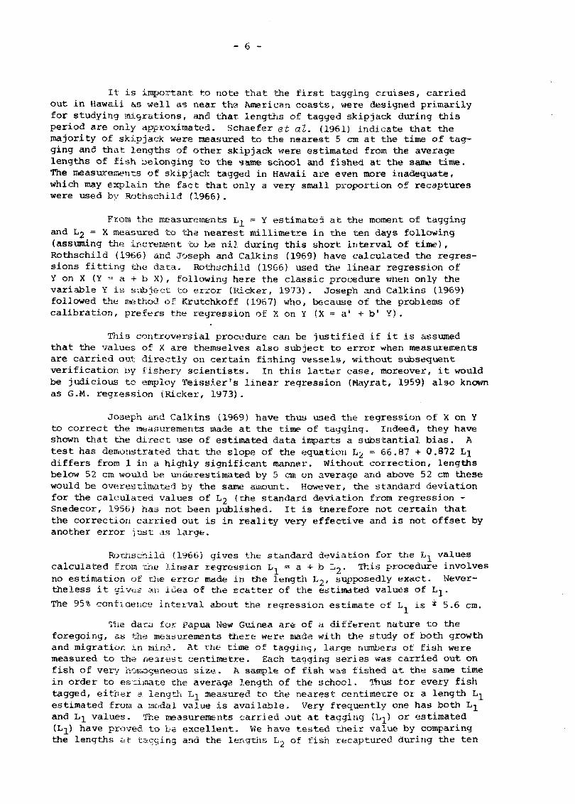
It is important to note that the first tagging cruises, carried out in Hawaii as well as near the American coasts, were designed primarily for studying migrations, and that lengths of tagged skipjack during this period are only approximated. Schaefer et al. (1961) indicate that the majority of skipjack were measured to the nearest 5 cm at the time of tagging and that lengths of other skipjack were estimated from the average lengths of fish belonging to the same school and fished at the same time. The measurements of skipjack tagged in Hawaii are even more inadequate, which may explain the fact that only a very small proportion of recaptures were used by Rothschild (1966).
From the measurements L^ = Y estimated at the moment of tagging and L12 = X measured to the nearest millimetre in the ten days following (assuming the increment to be nil during this short interval of time), Rothschild (1966) and Joseph and Calkins (1969) have calculated the regressions fitting the data. Rothschild (1966) used the linear regression of Y on X (Y == a + b X) , following here the classic procedure when only the variable Y is subject to error (Kicker, 1973). Joseph and Calkins (1969) followed the method of Krutchkoff (1967) who, because of the problems of calibration, prefers the regression of X on Y (X = a' + b' Y).
This controversial procedure can be justified if it is assumed that the values of X are themselves also subject to error when measurements are carried out directly on certain fishing vessels, without subsequent verification by fishery scientists. In this latter case, moreover, it would be judicious to employ Teissier's linear regression (Mayrat, 1959) also known as G.M. regression (Ricker, 1973).
Joseph and Calkins (1969) have thus used the regression of X on Y to correct the measurements made at the time of tagging. Indeed, they have shown that the direct use of estimated data imparts a substantial bias. A test has demonstrated that the slope of the equation L2 = 66.87 + 0.872 Lj differs from 1 in a highly significant manner. Without correction, lengths below 52 cm would be underestimated by 5 cm on average and above 52 cm these would be overestimated by the same amount. However, the standard deviation for the calculated values of L2 (the standard deviation from regression -Snedecor, 1956) has not been published. It is tnerefore not certain that the correction carried out is in reality very effective and is not offset by another error just as large.
Rothschild (1966) gives the standard deviation for the L^ values calculated from the linear regression L, = a + b L2- This procedure involves no estimation of the error made in the length L->, supposedly exact. Nevertheless it givt;£ an iuea of the scatter of the estimated values of Lj.
The 95% confidence interval about the regression estimate of L.. is * 5.6 cm.
The da-cu for Papua New Guinea are of a different nature to the foregoing, as the measurements there were made with the study of both growth and migration in mind. At the time of tagging, large numbers of fish were measured to the nearest centimetre. Each tagging series was carried out on fish of very homogeneous size. A sample of fish was fished at the same time in order to estimate the average length of the school. Thus for every fish tagged, either a length L^ aeasured to the nearest centimetre or a length L^ estimated from a modal value is available. Very frequently one has both L^ and L^ values. The measurements carried out at tagging (L- ) or estimated (Lj) have proved to be excellent. We have tested their value by comparing the lengths at tagging and the lengths L? of fish recaptured during the ten

- 7 -
days following. The values of the lengths L- used for control were verified by those responsible for the tagging programme. The body of data used to verify the adequacy of the measurements appears in Table I of Annex I.
We have simply calculated the mean values of x = L2 - L- and x' = L2 - L^ with their confidence intervals.
The following mean values have been obtained:
x = + 0.509 At a confidence level of 95%: - 0.464 (N = 67)
x'= + 0.452 At a confidence level of 95%: - 0.654 (N = 69)
For measurements carried out to the nearest centimetre it may thus be assumed that there is practically no error of measurement at tagging, the more so as there will nonetheless be a certain amount of growth between the first and tenth days of liberty. Moreover we have verified that the use of a linear regression between the parameters L^ and L2 on the one hand and L^ and Lj on the other, did not produce any improvement in the measurements, but on the contrary involved a not insignificant risk of error (Table II, Annex I).
Furthermore, having both values, measured and estimated L^ and L,, for 423 skipjack we have calculated the mean value of x = L^ - L-. . We have found x = 0.38 + 0.20 cm at the 95% confidence level. These results confirm that tagging in Papua New Guinea has been carried out for the most part on groups of very homogeneous size class fish (Lewis, personal communication).
We have postulated that the annual growth AL_ is a function of the At
length L at time of tagging, as well as the time At spent at large. Taking into account the size of the fish at the time of tagging and after the time at large, we have regrouped the data by zones, by 5 cm size classes and for fish which had been roughly the same length of time in the sea. We were thus able to assemble data for fish which had been in the sea from two to five months, from five to twelve months and for more than a year. We purposely omitted from this study data for skipjack which had been at large for less than two months. With the errors in estimating lengths at time of tagging being often greater than the value of the increments AL for periods of less than two months, a not inconsiderable proportion of the values AL = L2 - 1J\ are, and this is quite logical, mathematically negative. This can be readily verified for the eastern Pacific by examining the skipjack growth curves in Figure 9 of the Annual Report for 1959 of the IATTC (Anon., 1960). The negative increments, which are in conflict with simple logic, have everywhere had a very clear tendency to disappear from the data for a variety of reasons and without it being easy to estimate the bias thus introduced into the results.
The body of data which we have used appears in Annex I: Tables III, IV, V, VI and VII. For skipjack which were at large for two to five months and for five to twelve months we have calculated the mean annual growth increments m = AL for each size class. The confidence interval of
W the means m has been e s t ima ted by + t (S tuden t ' s t ) for the small
~ 1 / —
samples s (n < 30) . For the samples of l a r g e r s i z e , the formula used was
m ± e / n (Schwartz, 196 3) .

- 8 -
The collected results obtained appear in Tables 1 and 2. In the Pacific the lowest growth rates were observed in Papua New Guinea and the highest in Hawaii. Since the confidence intervals for the estimation of m largely tally, we have made test comparisons of the means, two by two, for each size class.
The comparison between two means m_ and nv observed for n_ > 30 a b a
and n > 30 is based on:
ma ~ "b
. 2 2 /s + s, a b
' n + n, a b In the case of the other samples we used Student's t test where:
2 2 m _ m, , 2 Z (m-m ) + E (m-m)
t = a b and s = a b
2 2 n + ri s s a D n "b
Tables 3 and 4 present the results of the different tests. One cannot say with complete confidence that there are differences among the data groups.
The study rests, in fact, on few data in each group. The confidence intervals for m are only small for a large number of data (n > 30).
Moreover, in calculating the means and in comparing them group by group, we implicitly assumed that we were dealing with data taken at random in normal distributions. This is obviously a crude approximation. Our efforts at homogenization of the data are of limited application. For example, in the 40-45 cm group the data might fall between 40 and 41 cm in one tagging area and between 44 and 45 cm in another. Thus if the increments in the months following are significantly different, this should not cause surprise.
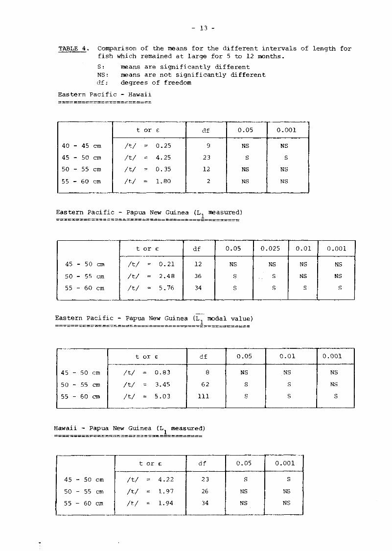
The length estimation errors made at time of tagging may be amply sufficient to produce significant differences. The example of skipjack tagged in Papua New Guinea and which remained in the sea for five to twelve months (Table 4) is especially instructive in this regard. Indeed, according to whether the measured length values L^ are used or those estimated from the modal value L,, the mean growths obtained are significantly different for tagged skipjack measuring between 55 and 60 cm.
This observation is particularly important when one considers the margin of error involved in skipjack length estimation for certain tagging series.
The artificiality of the divisions should also be emphasized. In our schema the increments of skipjack whose length at tagging time was estimated as 49.9 cm have not been compared with the increments of skipjack whose length at tagging was 50.1 cm. In the same way, the length increments of fish which remained five months in the sea are not directly compared with those of fish which were at large for six months.

TABLE 1. Mean value of annual growths m calculated for each 5 cm interval of length a time at large of 2 to 5 months. In each interval, besides the mean m,
and the confidence levels 90 and 95% appear, as well as the number o
L e n g t h a t t a g g i n g r e l e a s e
40 - 45 cm
45 - 50 cm
5 0 - 55 cm
5 5 - 6 0 cm
6 0 - 6 5 cm
E a s t P a c i f i c JOSEPH a n d
CALKINS ( 1 9 6 9 )
n m s
90% 95%
n m s
90% 95%
n m s
90% 95%
n m s
90% 95%
n m
5 2 0 . 2 2
8 . 6 0 + 8 . 2 0 + 1 0 . 6 7
14 1 5 . 0 1 1 1 . 8 7 + 5 . 6 2 + 6 . 8 5
6 1 1 7 . 7 8
9 . 9 2 + 2 . 0 9 + 2 . 4 9
6 1 2 . 5 2
9 . 1 7 + 7 . 5 4 + 9 . 6 2
1 7 . 1 8
P a p u a New G u i n e a L.. ( m e a s u r e d t o t h e
n e a r e s t cm)
n m s
90% 95%
n m s
90% 95%
n m s
90% 95%
n m s
90% 95%
3 1 3 . 4 6
9 . 6 2 + 1 6 . 2 3 + 2 3 . 9 1
26 7 . 6 5 8 . 5 3
+ 2 . 8 6 + 3 . 4 5
39 7 . 1 9 9 . 8 3
+ 2 . 5 9 + 3 . 0 9
3 5 . 9 5 2 . 4 8
+ 4 . 1 8 + 6 . 1 6
P a p u a New G u i n e
L : e s t i m a t e d f t h e m o d a l v a
n m s
90% 95%
n m s
90% 95%
n m s
90% 95%
n m s
90% 95%
3 2 0 . 1 2
3 . 9 2 + 6 . 6 1 + 9 . 7 4
39 8 . 1 4 9 . 3 5
+ 2 . 4 6 + 2 . 9 3
4 1 6 . 5 1
1 3 . 4 5 + 3 . 4 6 + 4 . 1 2
3 3 . 7 5 9 . 0 0
+ 1 5 . 1 8 + 2 2 . 3 6

TABLE 2. Mean value of annual growths m calculated for each 5 cm interval of lengt a time at large of 5 to 12 months. In each interval, besides the mean m
s and the 90 and 95% confidence limits appear, as well as the number
Length a t t a g g i n g r e l e a s e
35 - 40 cm
40 - 45 cm
45 - 50 cm
50 - 55 cm
55 - 60 cm
60 - 65 cm
E a s t P a c i f i c JOSEPH AND CALKINS
(1969)
n m
n m s
90% 95%
n m s
90% 95%
n m s
90% 95%
1 21 .82
7 1 1 . 0 3
6 . 9 9 + 5 . 1 4 + 6 . 4 7
12 12 .46
6 . 9 4 + 3 .60 + 4 . 4 1
3 15 .26
2 . 3 2 + 3 .92 + 5 . 7 7
Hawai i ROTHSCHILD
(1965)
n m
n m s
90% 95%
n m s
90% 95%
n m s
90% 95%
n m
1 2 3 .10
10 2 3 . 6 7
7 .00 + 4 . 0 6 + 5 . 0 1
18 2 1 . 9 7
5 .29 + 2 . 1 6 + 2 . 6 2
2 1 4 . 3 3
8 . 2 1 + 3 6 . 6 5 + 7 3 . 7 6
1 1 0 . 4 3
Papua New Guinea L (measured t o t h e
n e a r e s t cm)
n m s
90% 95%
n m s
90% 95%
n m s
90% 95%
n m s
90% 95%
7 11 .76
5 .80 + 4 . 2 6 + 5 . 3 7
26 7 . 9 8 4 . 1 8
+ 1.40 + 1.69
33 3 .90 3.32
+ 0 . 9 8 + 1.18
4 2 . 6 2 2 . 8 2
+ 3 .32 + 4 . 4 8
Papua N L : e s t i
t h e m
n m
n m s
90% 95%
n m s
90% 95%
n m s
90% 95%
n m s
90% 95%

- 11 -
TABLE 3. Comparison of the means for the different intervals of length for fish which remained at large for 2 to 5 months.
S: means are significantly different NS: means are not significantly different df: degrees of freedom
Eastern Pacific - Papua New Guinea (L measured)
45 -
50 -
55 -
60 -
- 50 cm
- 55 cm
- 60 cm
- 65 cm
A/ /t/
A/ A/
t or e
= 0.21
= 4.54
= 1.25
= 0.43
df
15
85
43
2
0.05
NS
S
NS
NS
0.001
NS
s NS
NS
Eastern Pacific - Papua New Guinea (L modal value)
45 - 50 cm
50 - 55 cm
55 - 60 cm
60 - 65 cm
A/ A/ A/ A/
t or e
= 0.72
= 4.91
= 1.05
= 0.33
df
15
X
45
2
0.05
NS
S
NS
NS
0.001
• NS
s NS
NS
Papua New Guinea (L measured) - Papua New Guinea (Ln modal value)
45 - 50 cm
50 - 55 cm
55 - 60 cm
60 - 65 cm
A/ A/ A/ A/
t or e
= 1.11
= 0.21
= 0.26
= 0.41
df
4
63
X
4
0.05
NS
NS
NS
NS

- 12 -
TABLE 3. (cont.)
Eastern Pacific - Atlantic
40 - 45 cm
45 - 50 cm
50 - 55 cm
55 - 60 cm
t or e
A / = 0.97
A / = 0.83
A / = 0.46
A / = 0.54
df
4
13
62
6
0.05
NS
NS
NS
NS
Papua New Guinea (L measured) - Atlantic
45 - 50 cm
50 - 55 cm
55 - 60 cm
t or e
A / = 1.05
A / = 1.25
A / = 1-28
df
2
27
39
0.05
co co
to
2
Z
Z
Papua New Guinea (L modal value) - Atlantic
45 - 50 cm
50 - 55 cm
55 - 60 cm
t or e
A / = 1.12
A / = 1.14
A / = 1.01
df
2
40
41
0.05
NS
NS
NS
- 13 -
TABLE 4. Comparison of the means for the different intervals of length for fish which remained at large for 5 to 12 months.
S: means are significantly different NS: means are not significantly different df: degrees of freedom
Eastern Pacific - Hawaii
40 -
45 -
50 -
55 -
45 cm
50 cm
55 cm
60 cm
t o r e
A / = 0 . 2 5
A / = 4 .25
/ t / = 0 . 3 5
A / = 1-80
d f
9
2 3
12
2
0 . 0 5
NS
S
NS
NS
0 . 0 0 1
NS
s NS
NS
Eastern Pacific - Papua New Guinea (Ln measured)
45 -
50 -
55 -
- 50 cm
- 55 cm
- 60 cm
t o r e
A / = 0 . 2 1
A / = 2 . 4 8
A / = 5 .76
d f
12
36
34
0 . 0 5
NS
S
S
0 .025
NS
S
S
0 . 0 1
NS
NS
S
0 . 0 0 1
NS
NS
s
Eastern Pacific - Papua New Guinea (L modal value)
45 -
50 -
55 -
- 50 cm
- 55 cm
- 60 cm
t o r e
A / = 0 . 8 3
A / = 3 .45
A / = 5 . 0 3
d f
8
6 2
1 1 1
0 . 0 5
NS
S
S
0 . 0 1
NS
S
S
0 . 0 0 1
NS
NS
S
Hawaii - Papua New Guinea (L measured)
4 5 - 50 cm
5 0 - 55 cm
55 - 60 cm
t o r e
A / = 4 . 2 2
A / = 1 - 9 7
A / = 1-94
d f
2 3
26
34
0 . 0 5
S
NS
NS
0 . 0 0 1
S
NS
NS

- 14 -
TABLE 4. (cont.)
Hawaii - Papua New Guinea (L.. modal value)
40 - 45 cm
45 - 50 cm
50 - 55 cm
55 - 60 cm
t or e
A / = 1.89
A / = 2.25
A / = 2.22
A / = 1-50
df
9
19
52
109
0.05
NS
S
S
NS
0.025
NS
NS
NS
NS
Papua New Guinea (L1 measured) - Papua New Guinea (L modal value)
45 - 50 cm
50 - 55 cm
55 - 60 cm
60 - 65 cm
t or e
A / = 0.78
A / = 1-06
/e/ = 2.08
A / = 1.51
df
8
76
X
7
0.05
NS
NS
S
NS
0.025
NS
NS
NS
NS

- 15 -
The methods of analysis of the data are also involved in the various results obtained for the growth means. Thus Schaefer et al. (1961) have shown that in using a straight line Al = a + b At, whether passing or not through the origin, for the regression between the increment Al in mm and the time at liberty At in days, the mean increments in their size intervals differed appreciably (Table 5). If the Papua New Guinea data of Table 1 are regrouped into the same size intervals as those employed by Schaefer et al. (1961), the results for the fish which remained at liberty for 2 to 5 months are obtained (Table 6). The growths obtained in Tables 5 and 6 are of the same order of magnitude.
The data used by Schaefer have a 90% correspondence with those of fish which remained in the sea from 0 to 6 months. His results are thus roughly comparable to those which we have obtained for skipjack which remained for 2 to 5 months in the sea in Papua New Guinea. These results lend support to the preceding hypothesis of results not significantly different from one tagging zone to another. A global approach such as that which Schaefer et al. (1961) had in mind has been adopted in calculating the linear regression Al = a + b At for the total number of skipjack which remained in the sea for 2 to 5 months in Papua New Guinea and in the eastern Pacific (IATTC zone) .
Al being expressed in cm and At in days, the two following regressions have been obtained:
Eastern zone (IATTC) : Al = 1.4683 + 0.03055 At
Papua New Guinea zone : Al = -0.8049 + 0.03151 At
These correspond to a mean increment of 12.61 cm for the eastern Pacific and 10.69 cm for Papua New Guinea.
The two values of a are not significantly different from 0 and neither are the slopes significantly different from one another. Nevertheless, too hasty a conclusion should not be drawn as to the equality of the results because the variances s and s, are very high. For fish which
a b x
remained at large in Papua New Guinea for 5 to 12 months, we have obtained the following equation for the linear regression:
Al = -0.1697 + 0.01585 At
which would correspond to an annual increment of 5.62 cm per annum. The variability of the increment data utilized is such that this latter line is not significantly different from the two preceding ones.
As regards skipjack at large for more than a year, our data permit no valid comparison between zones. We can merely give the results obtained in Papua New Guinea (Table 7).
The mean size at recapture of the few tagged skipjack between 55 and 60 cm and recaptured in the Papua New Guinea zone after an interval of more than two years was 62 cm.

- 16 -
TABLE 5. Estimation of the growth of skipjack from recapture data.
IATTC data for recaptures to 31 October 1959.
S i z e a t t a g g i n g r e l e a s e
400-499 mm
500-599 mm
600 and above
A l l s i z e s
R e g r e s s i o n o f t h e growth i n c r e m e n t i n mm on t ime a t l a r g e i n days
N b Annual i n c r e m e n t
29 0 .475 173 mm
82 0 .290 106 mm
28 0 .160 58 mm
139 0 . 3 4 1 124 mm
R e g r e s s i o n p a s s i n g t h r o u g h t h e o r i g i n
b Annual i n c r e m e n t
0 . 5 6 7 207 mm
0 . 3 1 8 116 mm
0 .00 3 1 mm
0 .335 122 mm
(SCHAEFFER et at. , 1961)

- 17 -
TABLE 6. Annual increments calculated in centimetres for skipjack which remained at large for 2 to 5 months in Papua New Guinea.
Length classes
40 - 50 cm
50 - 60 cm
> 60 cm
Measurements at tagging release
Length L measured to the nearest cm
13.46 cm
n = 3
7.37 cm
n = 65
5 .95 cm
n = 3
L estimated from the modal value
20.12 cm
n = 3
7.30 cm
n = 80
3.75 cm
n = 3
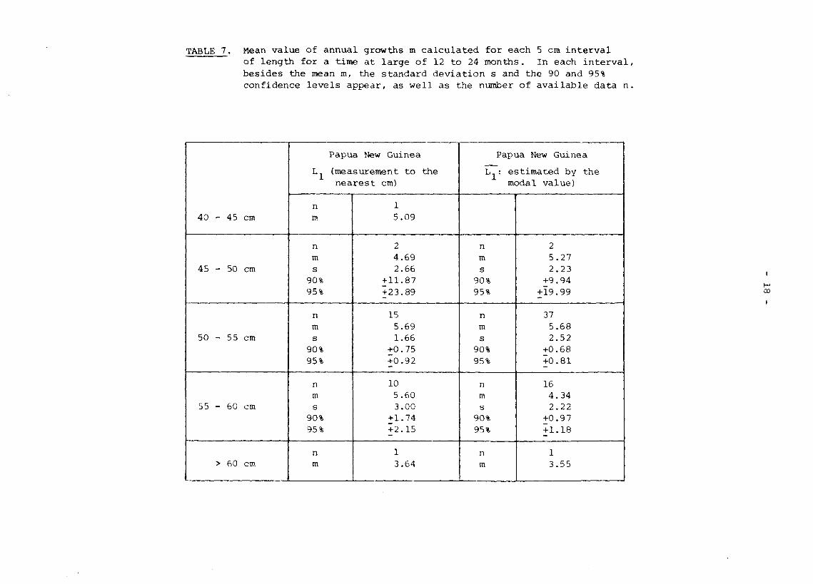
TABLE 7. Mean value of annual growths m calculated for each 5 cm int of length for a time at large of 12 to 24 months. In each besides the mean m, the standard deviation s and the 90 and confidence levels appear, as well as the number of availabl
40 - 45 cm
4 5 - 50 cm
50 - 55 cm
5 5 - 60 cm
> 60 cm
P a p u a New G u i n e a
L 1 ( m e a s u r e m e n t t o t h e n e a r e s t cm)
n m
n m s
90% 95%
n m s
90% 95%
n m s
90% 95%
n m
1 5 . 0 9
2 4 . 6 9 2 . 6 6
+ 1 1 . 8 7 + 2 3 . 8 9
15 5 . 6 9 1 .66
+ 0 . 7 5 + 0 . 9 2
10 5 . 6 0 3 . 0 0
+ 1 . 7 4 + 2 . 1 5
1 3 . 6 4
P a p u a New G u i n e
L : e s t i m a t e d b y m o d a l v a l u e )
n m s
90% 95%
n m s
90% 95%
n m s
90% 95%
n m
2 5 . 2 7 2 . 2 3
+ 9 . 9 4 + 1 9 . 9 9
37 5 . 6 8 2 . 5 2
+ 0 . 6 8 + 0 . 8 1
16 4 . 3 4 2 . 2 2
+ 0 . 9 7 + 1 . 1 8
1 3 . 5 5

- 19 -
We note that of the 660 fish recaptured, about thirty had escaped from the coastal zone and had moved north of the equator dispersing along the equatorial convergence as far as longitude 172 W, which was the eastern limit of Japanese fishing activity in 1972-1974 (Figure 2). Some skipjack might quite possibly have gone even further east, since it is hard to see what ecological barrier would halt them at 17 2 W.
It seems that the skipjack which set out into the open ocean had a more rapid growth rate then those which remained in the coastal waters. But the data do not allow this to be stated as fact. However, this idea that there is a different rate of growth in the coastal zone as compared with the open sea is an interesting one to follow. The recapture at Hawaii of 16 skipjack tagged in open waters off California and of one skipjack tagged in open water off Japan (Table 8) lends support to the hypothesis of a more rapid growth of fish which have escaped from the coastal zone.
Japanese fishing data (Tanaka, 1976-1977) show that large quantities of skipjack of 8 to 10 kg are found in the open ocean along the equatorial convergence from 145 R to 170 E, whereas in the coastal zones of Papua New Guinea, the Philippines and Japan, the skipjack fished rarely exceed a length of 60 cm.
A very general hypothesis could be proposed that suggests there exist a number of spatio-temporal "ecological compartments", more or less favourable, and within which the biological parameters of the skipjack (growth, natural mortality, etc) would be adapted to the environmental conditions. This hypothesis has already been formulated by Kearney (1976) in a different form.
Here, the skipjack is assumed to pass more or less en masse from one compartment to another. The "coastal compartment" of Papua New Guinea could in this case be regarded as comparatively tight (for exit) since only some thirty fish out of 660 recaptured departed from it to head in the direction of the equatorial convergence without, however, crossing it. We note that any migration towards the south was not discernible during the period of the tagging programme due to the absence of fishing.
Tagging recapture data for the Pacific as a whole have not demonstrated any very important exchanges between distant geographic zones, insofar as the exploited phase of the population (or populations) is concerned.
Nevertheless, these exchanges do take place on a large scale, since fish marked on either side of the Pacific may turn up in Hawaii.
Growth seems to come to a halt in the coastal zones at around 60-65 cm and to continue to 80 cm and beyond in the zones of the open ocean such as Hawaii.
A bias may have led to underestimation of growth in Papua New Guinea. Recaptures were made essentially by pole-and-line vessels which are very selective for coastal fish. The distribution and frequency of pole-and-liners and of seiners, drawn up for a number of years at IATTC, are of interest in this connection. The seiners can take distinctly larger skipjack than the pole-and-liners. Captures of skipjack of more

TABLE 8. Recapture data for skipjack tuna tagged by IATTC, presented at the meeting of the group of experts of the IPFC at Manila, 1-2 March 1978.
Date
R e c a p t u r e
6 - 1 2 - 6 2
8 - 2 2 - 6 2
4 - 0 5 - 6 3
6 - 2 7 - 6 7
7 -21 -70
8 -08 -70
9 - 0 1 - 7 6
9 - 0 1 - 7 6
* 8 - 2 2 - 7 6
* * 1 2 - 0 9 - 7 6
6 - 1 0 - 7 7
6 - 2 8 - 7 7
7 - 2 6 - 7 7
7 -29 -77
8 - 1 9 - 7 7
9 - 1 4 - 7 7
9 - 2 0 - 7 7
T a g g i n g -r e l e a s e
9 - 0 5 - 6 0
4 - 1 7 - 6 0
9 - 2 2 - 6 1
6 - 0 5 - 6 5
1 1 - 0 6 - 6 9
1 1 - 0 6 - 6 9
7 - 0 6 - 7 5
7 - 2 0 - 7 5
7 -06 -75
5 - 1 7 - 7 6
6 - 1 7 - 7 6
6 - 1 8 - 7 6
1 0 - 0 4 - 7 6
6 - 1 7 - 7 6
6 - 1 8 - 7 6
6 - 1 7 - 7 6
6 - 1 7 - 7 6
Days a t
l i b e r t y
6 4 6
8 5 8
5 6 1
75 3
258
276
422
4 0 8
4 1 0
206
357
375
295
4C7
4 2 7
4 5 4
4 6 0
P o s i t i o n
R e c a p t u r e
Hawai i
Idem
C h r i s t m a s I s .
Hawai i
Idem
Idem
M o l o k a i , Hawai i
So . o f P e a r l Hbr .
21°14 , N-171°51 , W
W a i a n a e , Hawai i
Kahuku, Hawai i
Kaneohe , Hawai i
Idem
Idem
Hawai i
B a r b e r s P t . , Hawai i
W a i a n a e , Hawai i
T a g g i n g - r e l e a s e
Ba j a CA
R e v i l l a g i g e d o I s .
Ba j a CA
R e v i l l a g i g e d o I s .
C l i p p e r t o n I s ,
Idem
Ba ja Madga l ena , CA
Cabo San L u c a s , CA
24°07 , N-113°45 , W
3 1 ° 5 7 , N - 1 5 9 ° 1 2 ' E
21°16 , N-111°04 , W
21°07 , N-111°16 , W
25°45 , N-112°47 , W
21°16 , N-111°04 , W
21°07 , N-111°16 , W
21°16 , N-111°04 , W
Idem Idem
F o r k - l e n g t
R e c a p t u r e
77 .4
7 8 . 0
7 0 . 0
8 1 . 4
7 0 . 3
7 1 . 5
7 2 . 7
7 5 . 1
8 0 . 0
6 8 . 0
7 3 . 0 - 7 5 . 0
7 6 . 0
7 2 . 3
75 .0
7 4 . 9
7 6 . 0
7 5 . 2
* Recaptured by a Japanese vessel ** Tagged by Japanese fishery scientists

- 21 -
than 65 cm, common for the seiners, are very much rarer for the pole-and-line boats. Moreover the factor "distance from the coast" for the two types of vessel may play a part, being superimposed on the intrinsic selectivity of each type of fishing gear.
When growth curves or key lengths-for-age are being established, another possible source of error is worth pointing out. Scientists interpreting recapture data have assumed (as we have) that growth is a function of the length of the fish at the time of release. In fact, it is also a function of age. When growth is slow there is thus more risk that fish of a given size class are derived from different age groups. This risk is greater if tagging is done on relatively aged fish, the range of sizes increasing with age. If there are several possible ages for the same size, one may find several types of growth for this same size.
In Figure 3 we have drawn up the histograms of frequencies of the annual growth races Al_ for fish of 50 to 55 cm and of 55 to 60 cm which
At remained at liberty for two to five months in Papua New Guinea. There would appear to be several modes in the growth rates. The small number of observations (26 and 33) does not allow any conclusion, but in future work it would be useful to study this phenomenon more closely, particularly in conjunction with counts of daily growth marks on the otoliths of recaptured fish.
In short, it can be said that the analysis of the growth data available in the approximately 45 to 60 cm range has shown slower mean growth for the skipjack of Papua New Guinea than for those of the eastern Pacific. Nevertheless, since the values obtained in the east and west are not significantly different, the results will need to be checked on the basis of more abundant and reliable data, particularly insofar as the eastern Pacific is concerned.
III. PETERSEN'S METHOD
A. General considerations
The method of length frequencies was, of course, introduced by Petersen (1892). It is worth recalling that this method consists of following the growth of some modal lengths as a function of time. "Much early work by d'Arcy Thompson and others, using Petersen's method, was later shown to be inaccurate because a succession of modes had been treated as belonging to successive year classes, when in fact they represented only dominant year classes which were separated by one or more scarce broods" (Ricker, 1958). Today some workers still use an analogous method which could be described as Petersen's method short-circuited. It consists of considering only a polymodal distribution of length frequencies and of making (generally in an implicit fashion) the hypothesis that the successive modal distributions, obtained by one of numerous methods of analysis presently available (Harding, 1949; Cassie, 1954; Partlo, 1955; Tanaka, 1956; Gheno and Le Guen, 1968; Daget and Le Guen, 1975), correspond likewise to fish of successive age classes.
Brock (1954), who was the first to study the growth of skipjack from length frequency distributions in the Pacific, used a method half-way between the Petersen and d'Arcy Thompson methods. He regrouped his

- 22 -
measurements by six-month periods making the (implicit) hypothesis that in each distribution the successive modal values correspond to fish of successive age classes. Unfortunately the time interval between the analysed frequency distributions definitely does not allow us to follow the progression of modes and to verify the validity of the hypothesis. There is nothing to allow us to state positively that no age class is missing from the distributions or that, on the contrary, there were several broods for the same year. Bessineton (1976), working on the growth of skipjack tuna in Tahiti,used a similar method, grouping his samples by year rather than by six-month periods. During the two years (June 1973 to July 1975) for which the sampling lasted, about 1,000 skipjack were measured each month. Bessineton (1976) noted that he had never measured fish between 70 and 75 cm. He was thus led to explicitly assume that at least one age class was not represented in the distributions. "It is necessary to note that between the last class (75 to 80 cm) and the smaller fish, there is a discontinuity in all of the samplings carried out, fish of 70 to 75 cm being completely absent from the catches for a period of one year. Fish of 57 cm of one year cannot thus be connected with those of 79 cm of the following year" (Bessineton, 1976).
The conclusions on growth differ considerably according to the various hypotheses. According to Brock (1954) skipjack reach the length of 80 cm at three years. According to Bessineton (1976), this size is reached towards the age of five years. The progression in time of the modal values used having been demonstrated by neither of the authors, a pviovl one can neither validate nor invalidate their hypotheses and their conclusions. It is nonetheless interesting that Bessineton (1976) has brought up directly, for the first time, the problem of the absence of age classes in a fishery and indirectly the problem of migrations.
A very large number of other studies based on the classic Petersen method have been carried out in the Pacific as well as in the Atlantic and Indian Oceans. Today there is a large body of length frequency distribution data available for critical study.
We have taken up certain data, published (Kawasaki, 1955a, 1955b, 196 3; Diaz, 1966; Marcille and Stequert, 1976) or placed at our disposal by various laboratories (NMFS Hawaii, IATTC La Jolla, ORSTOM, ISRA Dakar). The previously unpublished frequency distributions are in Annex II.
The possible analyses of polymodal distributions into successive unimodal distributions have been carried out using the method of successive maxima (Daget and Le Guen, 1975) which does not require the hypothesis of normality of distributions but only that of symmetry in relation to the mean value.
Analysis of all the available data demonstrates three things:
1) Clear progressions of modes for more than a few months are extremely difficult to demonstrate. Exceptionally it is possible to have apparently acceptable mode progressions for a duration of 12 to 18 months.
- 23 -
2) The apparent mode progression may give in a single region, in different years, growths which are rapid, slow, nil and even negative,,
3) The extremely subjective aspect of the method, as Joseph and Calkins (1969) have already emphasized, makes it an extremely questionable one.
In most cases workers fail to specify the "utilizable" part of the mode progressions used by them in the study of growth or the reasons for discarding parts of them. Marcille and Stequert (1976) clearly explained the subjective aspect of the choice made by them during a study on skipjack in the Indian Ocean, "We have therefore cried to follow a mode progression which was the most logical possible and which took no account of the actual importance of some of the modes in relation to the others. Such a method may seem seriously open to criticism since it leaves an important part to the interpretation of the biologist; we have used it, however, because from June 1974 to March 1975 no logical progression of a principal mode appeared in the total monthly samples" (Marcille and Stequert, 1976) .
In working with more abundant, data (Annex II) of much greater diversity of origin we have come (in the main) to the general conclusion that, with the length frequency distributions of skipjack available, the degree of reliance which can be placed on the Petersen method is not very high in view of its subjectivity.
This may be intrinsic to skipjack because of its biology (extended reproductive periods) and behaviour (migration, regrouping in schools of uniform size, catchability ....)„ It is certain, for example, that knowledge of the migratory patterns would allow a better interpretation of certain mode progressions. In this connection it is interesting to consider the length-frequency histograms for skipjack of the region north-west of Madagascar in the Indian Ocean (Figure 4) and to note the interpretation which Marcille and Stequert (1976) have given them.
"From June 1974 to March 1975, the modal size of catches did not progress with time, remaining always between 47 and 48 cm; a very slight regression of this mode could even be discerned. In this case, the study of growth becomes very difficult if not impossible and we are unable, moreover, to determine the number of year classes. The great constancy of the modes from June 1?74 is in apparent contradiction to their rather regular evolution observed from August 1973 to May 1974; it could be explained by a continuous flux of recruitment, growth and migration, the net result of which would be an apparent mode at 47-48 cm persisting for a long period of time and creating an impression of absence of growth in the stock. Let us examine in detail the behaviour of the size histograms between July and January 1975: in July, there appears to take place a recruitment of young individuals of 38 to 4 3 cm, although as yet they are not very numerous; in Augustf these individuals are caught in greater numbers and appeal' to form a mode at 42-43 cm, which from October to December progressively renews the apparent mode, eventually replacing it completely. During this same period, the individuals making up the initial apparent mode are thought to leave the fishing zone as they grow. Study of the catches of the pole-and-liners during this period affords us some additional indications corroborating such a hypothesis. In June and July the c.p.u„e. is fairly low (4,5 and 3.4 tonnes/day): subsequently it increases progressively from 5„2 t/day in August to 8.1 t/day in November, as the class recruited in June-July grows and contributes to the initial

- 24 -
apparent mode. In the months which follow (December-January) individuals start leaving the fishery and c.p.u.e. drops to 5.3 and later to 4.2 t/day" (Marcille and Stequert, 1976) .
It is certain that analogous configurations in the successions of modes may be differently interpreted in the presence or in the absence of migrations in fisheries as in those of Tahiti and Hawaii, for example (Brock, 1954; Bessineton, 1976).
B. Representativeness of the samples
The variability of results obtained by the Petersen method may also be closely related to the problem of the representativeness of the samples used. From the fish measured one is supposed to reconstitute the length frequency distributions of a stock. Le Guen (1972) has shown that sampling controls may have an essential bearing on one fundamental characteristic of the representative samples. "The essential characteristics of samples drawn from the same fish stock and which are representative of this fish stock will be identical frequency distributions ... There is a very convenient technique based on this principle for estimating the number n of fish to be measured in order to obtain a length frequency distribution acceptable to the biologist. One continues to measure fish until the distribution stabilizes" (Le Guen, 1972).
The Centre National d'Exploitation des Oceans (CNEXO) and the Polynesian Fisheries Service (Service des Peches de Polynesie) have been using a very interesting sampling system since 1973, for the skipjack tuna fishery in Tahiti. The fishery studied operates in what is virtually a 1 square in which the mean annual catch is 400 tonnes of skipjack. Since the end of 1973, whenever catches have been landed at Papeete and each time that it has been possible, 50 to 100 fish have been measured from one tuna boat chosen as far as possible at random. "Thus an average of 1,000 skipjack tuna per month have been measured from the 40 to 50 tuna boats which are based at the port of Papeete and which land some 400 tonnes of skipjack per annum" (Bessineton, 1976).
Measurements of skipjack are made to the nearest cm, for want of a better method, with a tape-measure giving a length which takes into account the contour of the body between the tip of the snout and the fork of the tail ("round" length = contour length = LR) which has to be converted to the standard fork-length (LF). A conversion table (LR - LF - weight) drawn up by Bessineton (1976) is to be found in Annex II, as well as the measurements carried out from July 19 73 to April 1978.
We thus possess data on a fishery which is perfectly localized and of which the rate of measurement of skipjack tuna varied from 10 to 20% from July 1973 to September 1977. This afforded an exceptional opportunity for a theoretical study of the representativeness of samples.
We firstly assumed that, with such a rate of sampling over so restricted a geographical area, the sample was necessarily representative of the 400 tonnes fished. Thus we considered that the 4,259 skipjack tuna measured from 62 landings during the first quarter of 1977 allowed the drawing up of a histogram of length frequencies representative of the total catch made during this quarter.

- 25 -
F o r e a c h of t h e 62 l a n d i n g s , we took t h r e e random s u b - s a m p l e s (w i th t h e a i d of an HP 97 programme) of 10 , 20 and 30 f i s h , from which
we r e c o n s t i t u t e d t h r e e new f r e q u e n c y d i s t r i b u t i o n s , c o m p r i s i n g r e s p e c t i v e l y 620 , 1 ,141 and 1,568 i n d i v i d u a l c o n t o u r l e n g t h s (LR). From t h e l e n g t h f r e q u e n c y d i s t r i b u t i o n o b s e r v e d f o r t h e 4 , 2 5 9 f i s h , t a k e n as r e f e r e n c e d i s t r i b u t i o n , we c a l c u l a t e d t h e t h e o r e t i c a l d i s t r i b u t i o n s f o r 6 20 , 1 ,141 and 1 ,568 s k i p j a c k . These t h e o r e t i c a l d i s t r i b u t i o n s compr i s e r e s p e c t i v e l y 38 , 41 and 41 l e n g t h c l a s s e s ( t o 1 cm) w i t h more t h a n 5 i n d i v i d u a l s i n each c l a s s . We h a v e u sed t h e y^- t e s t a d v o c a t e d by S n e d e c o r (1956) t o compare t h e t h r e e d i s t r i b u t i o n s r e c o n s t i t u t e d by random s a m p l i n g of 10 , 20 and 30 f i s h p e r s h i p w i t h t h e c o r r e s p o n d i n g t h e o r e t i c a l d i s t r i b u t i o n s .
2 The x t e s t s o b t a i n e d f o r 6 2 0 , 1 ,141 and 1,568 l e n g t h s r e s p e c t i
v e l y a r e 5 2 . 0 1 - 2 5 . 2 1 and 23 .17 fo r 37 .40 and 40 d e g r e e s of f reedom.
The p r o b a b i l i t y t h a t t h e new d i s t r i b u t i o n s w i l l be i d e n t i c a l w i t h t h a t of t h e 4 , 2 5 9 f i s h measu red w i l l t h u s b e :
9 7 . 5 t o 99% i f 30 f i s h a r e measured p e r s h i p sampled ; 95 t o 97.5% i f 20 a r e m e a s u r e d ; and l e s s t h a n 10% i f 10 a r e m e a s u r e d .
The c o n c l u s i o n , t h e r e f o r e , i s t h a t i n t h e s a m p l i n g i n p r o g r e s s i n T a h i t i t h e r e i s no need t o measu re 60 t o 100 f i s h p e r l a n d i n g a s 20 t o 30 measu remen t s would s u f f i c e t o sample t h i s c a t c h -
We a c c e p t e d t h a t t h e 6 2 l a n d i n g s sampled were a d e q u a t e l y r e p r e s e n t a t i v e of t h e e x p l o i t e d s t o c k . A second t e s t was c a r r i e d o u t t o a s c e r t a i n w h e t h e r t h e t o t a l number of l a n d i n g s t o be sampled c o u l d be r e d u c e d . For t h i s we took at random 10, 20 , 30 , 4 0 , 50 , 55 and 60 l a n d i n g s and c a l c u l a t e d as b e f o r e t h e t h e o r e t i c a l d i s t r i b u t i o n s which o u g h t t o be o b t a i n e d i f t h e s e d i s t r i b u t i o n s were i d e n t i c a l t o t h o s e o b t a i n e d f o r 4 , 2 5 9 f i s h .
2 The x t e s t s c a r r i e d o u t on t h e d i s t r i b u t i o n s gave t he f o l l o w i n g
r e s u l t s :
Number of l a n d i n g s t a k e n a t random from
a t o t a l o f 6 2
10 20 30 40 50 55 60
Number of f i s h
721 1,258 2 ,129 2 ,802 3 ,427 3 ,799 4 , 1 7 9
P r o b a b i l i t y of r e p r e s e n t i n g t h e i n i t i a l d i s t r i b u t i o n of 4 , 2 5 9
s k i p i a c k
0 % 0 % 0 % 5 %
25 % 95 % 99-5%
This second test carried out on the landings of the first quarter of 1977 would tend thus to prove that although it. is not necessary to measure more than 20 to 30 fish per landing to characterize the catch, it is on the other hand essential to continue to sample the largest possible number of landings.

- 26 -
We were thus led to study sampling strategy in greater depth. To this end we intensified sampling from October 1977 and from the end of February to the beginning of April 1978 we examined a maximum of catches landed at the port of Papeete. We succeeded in obtaining, in six weeks, 120 samples, with about twenty skipjack tuna measured on each occasion. Applying always the principle of identity of the representative distributions (Le Guen, 1972) we calculated the theoretical distributions for 40, 60 and 80 catches from the distribution obtained for the 120 catches. Random lots were drawn week by week to achieve homogenization.
2 The x tests carried out on the distributions obtained after five
random samples gave the following results:
Number of l and ings taken a t random from the 120
sampled
40 (33%) 60 (50%) 80 (66%)
P r o b a b i l i t y of ob t a in ing a d i s t r i b u t i o n i d e n t i c a l wi th t h a t of the 2,263 l eng ths
obta ined from 120 samples
1s t l o t
5% 99.5% 99.5%
2nd l o t
10% 75% 90%
3rd l o t
25% 90% 99%
4 t h l o t
5% 95%
97.5%
5 t h l o t
5% 90% 95%
mean
10% 90% 96%
We could have continued the drawing of lots to get a more accurate mean in each case, but this did not seem necessary for our purpose. We adopted a sampling strategy consisting of measuring 20 to 30 fish for the maximum of catches landed at Papeete. It proved necessary to sample about 50 to 60% of landings in order to feel confident that our sampling adequately represented the catch as a whole, which in turn is assumed to reflect the stock fished.
The fundamental interest of this study lies in the fact that it may account for the variability of the results obtained by the Petersen method. Indeed, once it is recognized that below a certain threshold of sampling the frequency distributions are most unlikely to represent the stock fished, one should not be surprised at results using the Petersen method with too small a sample. The set of histograms of contour length (LR) frequencies produced with the measurements from Tahiti has enabled us under apparently good conditions to follow the growth of skipjack tuna from the first age class appearing in the fishery in January-February with an average size of about 45 cm.
Assuming that we are dealing with a stable stock unaffected by the phenomena of emigration and immigration, the growth G of these recruits of 45 cm would be of the order of 15 cm per year (12 cm < G < 20 cm) . Beyond 60 cm the interpretation of growth is practically impossible by the classic Petersen method.
In Figure 5 we have plotted the modal values obtained in sampling boat by boat from 1 July 1976 to 31 January 1978. There are thus from 20 to 50 different modal values for each month. The distributions obtained for the Papeete tuna boats are practically all unimodal. In Tahiti, therefore, it is easy to see the effect which any substantial reduction in the sample size would have. It is sufficient to take at random each month 1, 2 ... n

- 27 -
tuna boats as shown above and to draw up the histograms of the frequencies obtained with the n sub-samples taken at random, Several samplings made with a single boat from 1 February 1977 to 1 February 1978 yielded growth results ranging from 6 cm to 20 cm per year. Some random samplings with five tuna boats per month gave growth results ranging from 9 cm to 29 cm per year.
Petersen's n<ethod is much more sensitive to low sampling when the fishery is temporary and covers only three to six months of the year.
Random samplings for the Tahiti data from August to November 1977, with a single boat sampled per month have given growths ranging from -2 to +28 cm per year for skipjack tuna., In taking, at random, five of the catches landed per month, the growths obtained varied from approximately 4 cm to 20 cm per year. This result is important because numerous estimations of "annual" growth rate are obtained on the basis of data covering only three to four months of observations. It would explain the considerable variations in tlr2 growth rate estimated by us using the data for the years 1951 to 1959 published by Kawasaki (1955a, b - 1963). The Japanese tuna fisheries were very seasonal at that time. For an estimated mean growth rate of 15 cui to 16 cm per ye£ir for skipjack tuna which wore initially 45 cm to 50 cm, the successive annual values ranged from 0 to 24 cm (see Table 9).
There is no question here of wanting to extrapolate the results for Tahiti to the entire assemblage of data available for the Pacific. Certainly, this limited geographical character is found within other fisheries (Hawaii; and New Zealand, for example) but fishing conditions there are vei'y different. We simply wished to pose the general problem of the representativeness of samples which, insofar as it has not been broached, leaves a doubt hanging over the results obtained by the Petersen method.
IV- FORMULATION OF THE GROWTH RESULTS
A. General remarks on von Bertalanffy's model
The mathematical formulation most frequently used in growth studies is the von F.ertalanffy model (1938). It proved convenient in population dynamics since it allowed ready integration of biological results into production models without toe much tedious calculation (Beverton and Holt, 1957) .
As Blanc and Laurec (1976) observe, "Another model may prove to be more efficient; thus in the case of the growth rates of juveniles, Gompertz's model is often preferable. Neither model is ever exhaustive in practice".
Today, whore the use of computers enables us to escape the drudgery of tedious calculations, it is necessary to be fully aware of the limits and dangers of von Bertalanffy"s model.
Too many biologists have acquired the habit of believing that where the results of their observations could be expressed in terms of mathematical formulae, these formulae remained valid beyond the limits of their observations. Numerous cases of extrapolation could be cited here in respect of growth. Knight (1968) was the first to emphasize the dangers of such extrapolations from von Bertalanffy's equation.

TABLE 9. Mode progressions taken from a study of Japanese data published for the western Pacific (Kawasaki, 1955a, b; 1963 For each year there appears:
- the month from which the mode progression can be establishe
- the month in which the mode progression ends;
- the modal values (in cm) for the first and the last month;
- the estimation of growth rates expressed in cm per year /Al At
>v Year
MonthK
J
F
M
A
M
J
J
A
S
0
Al At
1951
45 ! 47
55 ! 55
24 j 19
1
1952
49 ! 49
54 i 52
15 • 9
j
1953
48
54
24
1954
43
51
19
1955
44
53
22
1956
46
53
17
1957
49
52
7
1
45
45
0
- 29 -
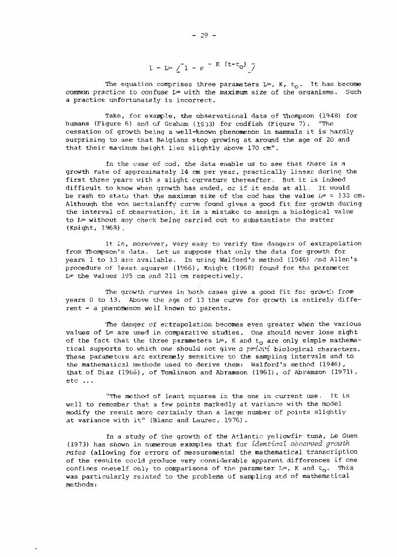
1 = L» /"l - e " K ( t _ to )_/
The equation comprises three parameters L°°, K, t0. It has become common practice to confuse I,00 with the maximum size of the organisms. Such a practice unfortunately is incorrect.
Take, for example, the observational data of Thompson (1948) for humans (Figure 6) and of Grahmu (1933) for codfish (Figure 7). "The cessation of growth being a well-known phenomenon in mammals it is hardly surprising to see that Belgians stop growing at around the age of 20 and that their maximum height lies slightly above 170 cm".
In the case of cod, the data enable us to see that there is a growth rate of approximately 14 cm per year, practically linear during the first three years with a slight curvature thereafter. But it is indeed difficult to know when growth has ended, or if it ends at all. It would be rash to state that the maximum size of the cod has the value L°° = 132 cm. Although the von Bertalanffy curve found gives a good fit for growth during the interval of observation, it is a mistake to assign a biological value to L°° without any check being carried out to substantiate the matter (Knight, 1963) .
It is, moreover, very easy to verify the dangers of extrapolation from Thompson's data. Let us suppose that only the data for growth for years 1 to 13 are available. In using Walford's method (1946) end Allen's procedure of least squares (1966), Knight (1968) found for the parameter L°° the values 195 cm and 211 cm respectively.
The growth curves in both cases give a good fit for growth from years 0 to 13. Above the age of 13 the curve for growth is entirely different - a phenomenon well known to parents.
The danger of extrapolation becomes even greater when the various values of L°° are used in comparative studies. One should never lose sight of the fact that the three parameters L°°, K and t0 are only simple mathematical supports to which one should not give a priori biological characters. These parameters are extremely sensitive to the sampling intervals and to the mathematical methods used to derive them: Walford's method (1946), that of Diaz (1966), of Tomlinson and Abramson (1961), of Abramson (1971), etc .. .
"The method of least squares is the one in current use. It is well to remember that a few points markedly at variance with the model modify the result more certainly than a large number of points slightly at variance with it" (Blanc and Laurec, 1976) .
In a study of the growth of the Atlantic yellowfir tuna, Le Guen (1973) has shown in numerous examples that for identical observed growth rates (allowing for errors of measurements) the mathematical transcription of the results could produce very considerable apparent differences if one confines oneself only to comparisons of the parameter L00, K and tQ. This was particularly related to the problems of sampling and of mathematical methods:
- 30 -
a) Different intervals of observation.
b) More or less good comparability of the methods used entailing large confidence intervals for the estimation of the parameters. The confidence intervals of K and L°° to the limit 0.95 obtained by Diaz's method for the growth of yellowfin tuna in the Congo, for example, were the following:
0.0169 < K < 0.0729
(The unit of time being the month)
156.4 < L» < 317.3 cm (Le Guen, 1973)
Let us note that within the intervals of observation the estimations of 1 = f (L°°, K, tQ) may be excellent and that as a result it is not von Bertalanffy's model that is called into question but rather its misinterpretation on the part of certain scientists.
"However well the von Bertalanffy curve may fit the code data, and in fact the fit is good, it is misleading to the reader to report any value for L°° at all, particularly if accompanied by an intimation that it represents the maximum size the fish can or does attain ... More important is the distorted point of view engendered by regarding L°° as a fact of nature rather than as a mathematical artifact of the data analysis" (Knight, 1968).
The comparison of different growth results should not, then, be made by direct comparison of the mathematical supports which are L°°, K and tQ, but from the growth rates obtained in the intervals of observation whether or not one employs the formula:
L - W " l - e " K (t-V_7
With Blanc and Laurec (1976) we can say that "if the constraints of publication already force the research worker to structure his thoughts, the demands of the mathematical model lead him even more to be rigorous when formulating the problem or setting down his conclusions".
B. Mathematical formulation of growth rates obtained from tagging studies
Taking into account the unresolved doubts on the other methods we consider that the best method available at present for the study of the growth of skipjack tuna is that of tagging-recapture. This is all the more true because the previous objection, that the growth rates obtained by tagging recapture are slower than those obtained by the Petersen method, no longer holds true seeing that the scientific validity of the Petersen method is challenged. Moreover, Lewis (1976) has shown in Papua New Guinea that the growth ring counts in tuna of the same size, both tagged and untagged, gave virtually identical results. It would be desirable to widen the scope of these latter observations to obtain confirmation of this important finding.
Notwithstanding the foregoing reservations it is quite true that von Bertalanffy's formula remains very useful for the description of growth rates, particularly when they are based on tagging-recapture where direct comparisons are practically impossible with the data available.
- 31 -
The available data being inconclusive, the approach to the growth curve must be made in ignorance of age. The method most used has, until recent years, been that of instantaneous increments due to Diaz (196 3) based on the formula: dl_ = K (L°°-?.) . It is difficult to accept that:
dt values Al and dj^ are comparable when the time that the skipiack have
At dt remained in the sea has been too long. Under these conditions it may be felt that one of the best approaches to growth rate to date has been made by Joseph and Calkins (1969) on the basis of 428 tagged fish, which had remained, on average, a short time in the sea.
Using two different mathematical treatments Joseph and Calkins (1969) found the following values for K and L°°:
1) K = 0.829 on an annual basis
L^ = 729 mm
2) K = 0 . 4 3 1 on an a n n u a l b a s i s
L00 = 881 mm
Joseph and Calkins have also provided an estimation of the confidence intervals for their results, giving as the upper and lower limits the two pairs of values:
1) K = 0 . 4 3 - L™ = 9 5 0 mm
2) K = 1 . 3 9 - L°° = 6 5 0 mm
The progress achieved in research on the biology and ecology of skipjack tuna gives rise to the hope that it will soon be possible to envisage a conclusive approach to the estimation of the parameters: K, L°° and t by assigning an age to the modal value of tagged skipjack for a group of fish of homogeneous size.
In the meantime we can make use of the first estimations of the age of young skipjack by Pannella's method. In Papua New Guinea, one-year-old skipjack were estimated to be approximately 40 to 45 cm long (Lewis, 1976). Legand's (1971) observations on the breeding period in the zone between New Caledonia and the Gilbert Islands show a very di stinct maximum of the gonadosomatic indices from January to April. The first modes visible in the length frequency distributions established on the tuna boats of New Caledonia are 42 and 38 cm in the periods January-March in J.974 and 1975 (Loubens, 1976). That is also in agreement with the observations of Kishinouye (1924) who estimated that the growth rate of juvenile tuna was of the order of 4 cm per month. With K and L°° one can calculate tQ knowing the age of the tuna for a given size.
In this paper our main purpose has been to compare the growth rates obtained in the Western and Eastern Pacific Ocean, without trying to estimate tQ.
From recapture data for skipjack tuna which had remained at large from two to five months, we established the parameters K and L<» for Papua New Guinea fish and for those of the Eastern Pacific (IATTC area). To do so we looked for the best fit of our data to the model:

- 32 -
. . - K At - K At, "lt + At = \ 6 + Loo (1 - e )
by the method of least squares (Abramson, programme BGC 4, 1971) . The following results were obtained:
1) Papua New Guinea: K = 0 . 9 4 5 1 ( a n n u a l b a s i s ) Loo = 6 5 4 . 7 mm
2) E a s t e r n P a c i f i c (IATTC a r e a ) : K = 0 . 6 3 7 1 L°° = 790 .6 mm
The variability of the increments observed means that the results are not significantly different. Moreover in the interval of the observations (40 to 60 cm) the estimations of increments by von Bertalanffy's formula give very comparable results for Papua New Guinea and the Eastern Pacific, as the computer printouts presented in Table 10 show. The calculated growth rate is however slightly slower in the west than in the east.
CONCLUSIONS
This publication makes no claim to be exhaustive, seeking only to raise the problems connected with the use of different techniques for estimations of growth. The general impression which emerges, however, is in favour of intensive tagging-recapture of skipjack tuna which should lead to acceptable estimations of growth, provided that measurements were made with care. Moreover, the migration data obtained through tagging-recapture may be expected to result in a better understanding of the modal progression of the Petersen method. Lastly, the interpretation of daily marks on the otoliths should assist in establishing key age-lengths or at least key "age group"-lengths which are necessary for further work on population dynamics. These three techniques, closely associated, are likely to appreciably improve determination of skipjack age.
The subject of the representativeness of samples goes well beyond the scope of the present study. The degree of confidence assigned, for example, to analysis of the data used for calculations of production is directly related to the representativeness of the samples measured at the landing of catches by the tuna boats.
When the conversion of length classes to age classes can be made only on the basis of von Bertalanffy's formula for growth, the method of analysis of the data is already unreliable enough where confidence intervals for the estimations of K, L°° and t are large. If, in addition, the length frequency distributions are not representative of the stock, the results of the various production and prediction calculations lose all credibility. A critical sampling threshold therefore needs to be determined, below which the level of sampling must not fall.

- 33 -
TABLE 10. Estimation of the parameters K and L°° in the Eastern (IATTC) and Western Pacific (Papua New Guinea) zones from tagging data. Growths calculated by von Bertalanffy's formula for the intervals of observations.
Eastern Pacific
Loo = 790.648 mm K = 0.6 37123 Number of increments used N = 87
Var (L°°) = 204.551 Var (K) = 0.124922 Covar (L°°, K) = -5.02030
Western Pacific
L°° = 654 .669 mm K = 0 .945120 N = 83
Var (Loo) = 24 .1596 Var (K) = 0 .249768 Covar (L°°, K) = - 2 . 3 7 6 6 4
Growths calculated
EASTERN PACIFIC WESTERN PACIFIC
4 0 . 0
4 2 . 4
4 4 . 7
4 6 . 8
4 8 . 8
5 0 . 7
52 .4
5 4 . 1
55 .6
57 .0
58 .4
5 9 . 7
6 0 . 9
6 2 . 0
6 3 . 1
4 0 . 0
4 2 . 3
4 4 . 4
4 6 . 3
4 8 . 0
4 9 . 6
51 .0
5 2 . 3
5 3 . 5
54 .6
55 .6
56 .5
5 7 . 3
58 .0
5 8 . 7
At (year)
0
.1
.2
. 3
.4
-5
.6
- 7
• 8
• 9
1.0
1.1
1.2
1.3
1.4

- 34 -
ACKNOWLEDGEMENTS
We should like to thank Dr Joseph, Director of IATTC, La Jolla, California, Mr Shomura, Director of the NMFS Laboratory in Hawaii and Mr Bour and his co-workers at ORSTOM - Africa, for the collection of skipjack tuna measurements placed at our disposal. We should also like to thank Mr de Chazeaux, Director of the Centre Oceanologique du Pacifique and Mr Stein, Director of the Service des Peches de Polynesie who communicated to us numerous data on the fishing of skipjack in Tahiti. We are especially indebted to Mr Wilson, Director of the Fisheries Service (Department of Primary Industry) at Konedobu in Papua New Guinea for permission to use the excellent results of the skipjack tagging programmes carried out by his Service from 1972 to 1974.
Finally, we should like to congratulate Mr Mariteraci, researcher with the Service des Peches, Tahiti, for all the work carried out at tuna landings. His samples have been of particular importance in our studies.

- 35 -
REFERENCES
Abramson, N.J. (1971). Computer program for fish stock assessment. FAO Fish. Teahn. Paper, No. 101, Program BGC4 (Tomlinson) 3 p.
Aikawa, H. (1937) . Notes of the shoal of bonito (Skipjack, Katsuuonus pelamis) along the Pacific Coast of Japan. Bull. Japan Soc. Sclent. Fisheries, vol. 6, No. 1, pp. 13-21.
Aikawa, H. and Kato, M. (1938). Age determination of fish (Preliminary report 1). Bull. Japan Soc. Scient. Fisheries, vol. 7, No. 1, pp. 79-88.
Allen, K.R. (1966a). A method of fitting growth curves of the von Bertalanffy type to observed data. J\ Fish. Res. Bd. Canada, 2 3(2), pp. 163-179.
Allen, K.R. (1966b). Fitting of von Bertalanffy growth curves, IBM 709, 7094, Fortran IV. Trans. Am. Fish. Soc, 95(2), pp. 231-232.
Anonymous (1960). Annual report for the year 1959. IATTC 3 La Jolla3
California, 156 p.
Anonymous (1976). Rapport du groupe de travail sur le listao atlantique. Dakar 22-27 mars 76. I.S.R.A. - O.R.S.T.O.M. - SSnegal.
Batts, B.S. (1972). Age and growth of the skipjack tuna, Katsuwonus pelamis (Linnaeus), in North Caro.lina Waters. Chesapeake Science, vol. 13, No. 4, pp. 237-244.
Bertin, L. (1958). Ecaille et sclerifications dermiques. Traite de Zoologie -Tome XIII, Masson et Cie, Paris, pp. 482-504.
Bessineton, C. (1976). La peche des bonitiers a Tahiti. C.N.E.X.O. Tahiti, C.0.P./1/PE 76002, 15 p. 2 annexes.
Beverton, R.J.H.. and Holt, S.J. (1957). On the dynamics of exploited fish populations. Fishery Invest. Lond. Series 2, 19, 533 p.
Blanc, F. and Laurec, A. (1976). De 1'heuristique au thaumaturgique en traitement des donnees d'ecologie marine. Cah. O.R.S.T.O.M.3 ser. OcSanogr., vol. 14, No, 2, pp. 101-107.
Brock, V.E. (1954). Some aspects of the biology of the aku, {Katsuwonus pelamis) in the Hawaiian Islands. Vac. Sai. 8, pp. 94-104.
Cassie, R.M. (1954). Some uses of probability paper in the analysis of size frequency distributions. Australian J. Marine and Freshwater Res., 5, pp. 513-522.
Chevey, P. (1933). The method of reading scales on the fish of the intertropical zone. Proa. 5th. Pacific. Sc. Congr. Toronto- 3818-3829.
Chi, K.S. and Yang, R„T„ (197 3) . Age and growth of skipjack tuna in the waters around the southern part of Taiwan. Acta Oceanographica Taiwanica, No. 3, pp. 199-222.
Clark, F.N. (1925). The life history of Leuresthes tenuis, an Atherine fish with tide controlled spawning habits. Fish. Bull-, Sacramento, No. 10, 51 p.

- 36 -
Daget, J . (1952). Bio logie e t c ro i s sance des especes du genre A l e s t e s , Bull. Inst. Fr. Afr. Noire, Dakar, v o l . 14, p p . 191-225.
Daget, J . and Le Guen, J . C . (1975). Les c r i t e r e s d 'age chez l e s p o i s s o n s . E x t r a i t de: Problemes d ' e c o l o g i e , Lamot te -Bour l i e re , Masson e t C ie . Editeurs, Paris, p p . 253-289..
Diaz, E.L. (1966) . Growth of sk ip jack tuna , Katsuwonus pelanris, i n the Eastern P a c i f i c Ocean. I.A.T.T.C. Intern. Report. No. 2, 18 p .
Gheno, Y. (1975). Nouvelle etude sur l a de te rmina t ion de l ' a g e e t de l a c ro i s sance de Sardinella aurita (Val) , dans l a region de Po in t e -No i re . Cah. O.R.S.T.O.M,, sir. Oceanogr., v o l . 13, No. 3, p p . 251-262.
Gheno, Y. and Le Guen, J . C . (1968). Determination de l ' a g e e t c ro i s sance de Sardinella eba (Val) , dans l a reg ion de Po in t e -No i r e . Cah. O.R.S.T.O.M., sir. Ocianogr., No. 1, pp. 70-82.
Graham, M. (1933). Report on the North Sea cod. Min i s t e r of Agr i cu l t u r e and F i s h e r i e s . Fish. Invest. London, 13 (4 ) , pp . 1-160.
Harding, J . P . (1949). The use of p r o b a b i l i t y paper for g r aph i ca l a n a l y s i s of polymodal frequency d i s t r i b u t i o n s . J. Marine Biol. Assn. U.K., 28(1 ) , p p . 141-153.
Joseph, J . and Ca lk ins , T.P. (1969) . Popula t ion dynamics of the skip jack tuna , Katsuwonus pelanris, of the Eas tern P a c i f i c Ocean. I .A.T.T.C. Bull., v o l . 13, No. 1, 273 p .
Kawasaki, T. (1955a). On the migra t ion and the growth of the s k i p j a c k , Katsuwonus pelanris (Linnaeus) , in the South Western Sea Area of Japan. Bull. Tohoku Regional Fisheries Research Laboratory, No. 4 , pp . 83-100.
Kawasaki, T. (1955b). On the migra t ion and the growth of the sk ip j ack , K. pelanris, in the IZU and BONIN Sea Areas and the North-Eastern Sea a rea along the P a c i f i c Coast of Japan . Bull. Tohoku Regional Fisheries Research Laboratory, No. 4 , p p . 101-119.
Kawasaki, T. (1963). The growth of sk ip jack on the Nor theas tern sea of Japan. Bull. Tohoku Regional Fisheries Research Laboratory, No. 23 , pp . 44-60.
Kearney, R.E. (1976). Some hypotheses on the skip jack resources of the P a c i f i c Ocean. Ad hoc Meeting of S c i e n t i s t s t o d i s c u s s Skipjack F i s h e r i e s Development and Research Requirements, Noumea, New Caledonia , 6-10 Dec. 76. S.P.C. No. 905/76, 13 p .
Kishinouye, K. (1924). Observat ion on the sk ip jack f i s h i n g grounds . Suisan Gakkai Hd 4 (2 ) , pp . 87-92.
Knight , W. (1968). Asymptotic growth: An example of nonsense d i sgu i sed as mathemat ics . J. Fish. Res. Bd. Canada, 25 (6 ) , p p . 1303-1307.
Krutchkoff, R.G. (1967). C l a s s i c a l and inverse r e g r e s s i o n methods of c a l i b r a t i o n . Technometrics 9 , pp . 425-440.

- 37 -
Legand, M. (1950). Con t r ibu t ion a l ' e t u d e des methodes de peche dans l e s t e r r i t o i r e s f r anca i s du Pac i f ique Sud. Journ. Soc. Ocean. T. VI, No. 6, pp. 141-184.
Legand, M. (1952). E t a t a c t u e l e t p e r s p e c t i v e s de l ' i n d u s t r i e du poisson dans l e s t e r r i t o i r e s f r anca i s du Pac i f ique Sud. Cybium - Mus. Nat. Hist. Nat. P a r i s No. 1, 23 p .
Legand, M. (1971). Donnees sur l a bon i t e a ven t re raye dans l e Sud Ouest Pacifique. Cah. O.H.S.T.O.M.3 ser. Oceanogv., vo l . 9, No. 4, pp . 403-409.
Le Guen, J . C . (1971). Dynamique des popula t ions de Fonticulus elongatus (Bowd. 1925). Po i s sons , Sc iaen idae , Cah. 0.R,S.T.O.M., ser. Oceanogv., v o l . IX, No. 1, pp . 3-84.
Le Guen, J . C . (1972). Stocks - Echant i l lonnage - Ef fo r t de Peche -Puissance de Peche - E x t r a i t du cours de dynamique des popu la t ions 1971-1972. Un ive r s i t e de Bretagne Occ iden ta le , Doc. Centre 0RST0M, Pointe-Noire, No. 22, 53 p .
Le Guen, J . C . (1973). Croissance des a lbacores (Tkunnus alhacaves) . Documents Scientifiques C.R.O. Abidjan., v o l . 4 , No. 3, pp. 1-28.
Le Guen, J . C . (1976). Age reading of i n t e r t r o p i c a l Sc iaenids by o t o l i t h method, seasonal and d a i l y p a t t e r n s . Cah. 0.R .0 .T.O.M., ser'. Oceanogr. , v o l . 14, No. 4, pp . 331-338.
Lewis, A.D. (1976). The re levance of da ta c o l l e c t e d in Papua New Guinea t o skipjack popula t ion s t u d i e s in the Western P a c i f i c . Doc. 1066/76, Department of Pvi-mavy Industry Papua. New Guinea, 5 p . 8 f i g .
Lewis, A.D. (1977). Tuna tagging in Papua New Guinea. Harvest, Papua. N&J Guinea. Vol. 4, No. 1, pp . 13-17.
Loubens, G. (1977). Observat ions on skipjack f i sh ing in New Caledonia. Ninth Regional Teclinical Meeting on F i s h e r i e s , S.P.C. Noumea, January 19 77.
M a r c i l l e , J . and S t e q u e r t , B. (1976). Etude p r e l i m i n a i r e de l a c ro i s sance du l i s t a o {Katsuwonus pelamts) dans I ' o u e s t de I 'Ocean Indien t r o p i c a l . Cah. O.R.S.T.O.M., ser. Oceanogr., v o l . 14, No. 2, pp . 139-151.
Mayrat, A. (1959). Nouvelle methode pour l ' e t u d e comparee d 'une c ro i s sance r e l a t i v e dans deux e c h a n t i l l o n s . Bull, Inst. Frang. Afr. Noire, 21 , 1, pp. 21-59.
Mol le r -Chr i s t ensen , J . (1964). Burning of o t o l i t h s , a technique for age de te rmina t ion of s o l e s and o t h e r f i s h . J. Cons. perm. int. Exp lor. Her, 29, pp . 73-81.
Monod, Th. (1950). Note sur la lecture des ecailles de quelques poissons du Niger moyen. C.R. Inter. Afrieanistes Ouest, Paris, vol. 1, pp. 204-206.
Pannella, G. (1971). Fish otoliths: daily growth layers and periodical patterns. Science N.Y., 173, 1124.

- 38 -
Pannella, G. (1973). Otolith growth patterns: an aid in age determination in temperate and tropical fishes. Proceedings of an International Symposium on: The Ageing of Fish. University of Reading, England, 19-20 July, 1973. Unwin Brothers Limited, pp. 28-39.
Partlo, J.M. (1955) . Distribution, age and growth of eastern Pacific albacore (T. alalunga Gmelin). J. Fish. Res. Bd. Canada, 12 (1), pp. 35-60.
Petersen, C.G.G. (1892). Fiskensbiologiske forhold i Holbock Fjord, 1890-1891. Beretning fva de Danske Biologiske Station, 1.
Poinsard, F. and Troadec, J.P. (1966). Determination de l'age par la lecture des otolithes chez deux cspeces de Sciaenidae ouest afrxcain (Pseudotolithus senegalensis C. et V. et Pseudotolithus typus Blkr). J. cons. Inter. Explor. Mer, 30, 3, pp. 291-307.
Postel, E. (1955) . La bonite a ventre raye (Katsuwonus pelamis) dans la region du Cap Vert. Bull. Inst. Prang. Afv. Noire. A, 17, 1202-14 (55/15 b).
Postel, E. (1963). Expose synoptique des donnees biologiques sur la bonite a ventre raye, Katsuwonus pelamts (Linn. 1758) (Atlantique et Mediterranee). F.A.0. Fisheries Reports, No. 6, 2, pp. 515-537.
Ricker, W.E. (1958). Handbook of computations for biological statistics of fish populations. Fish. Res. Board of Canada, Bull. No. 119, 300 p.
Ricker, W.E. (1973). Linear regression in fishery research. J. Fish. Res. Board Can. 30, pp, 409-434.
Rothschild, B.J. (1966). Estimates of the growth of Skipjack Tuna (Katsuwonus pelamts) in the Hawaiian Islands. 12th session I.P.F.C. Honolulu, Hawaii, U.S.A., 3-17 oct. 66. I.P.F.C./C66/Tech. 31.
Schaefer, M.B., Chatwin, B.M. and Broadhead, G.C. (1961). Tagging and recovery of tropical tunas, 1955-1959. I.A.T.T.C. Bull. vol. 5, No. 5, pp. 343-455.
Schwarts, D. (1963). Methodes statistiques a l'usage des medecins et des biologistes. Editions medicales Flarrmarion, Paris, 290 p.
Shabotiniets, E.I. (1968). Opredelenie vozrasta tuntosov Indiiskogo okeana TRUDY V.N.I.R.O., vol. 64: Trudy Azoher N.I.R.0. 28, pp. 374-376.
Snedecor, G.W. (1956). Statistical methods applied to experiments in agriculture and biology. The Iowa State University Press. Ames. U.S.A. 534 p.
Tanaka, S. (1956) . A method of analysing the polymodal frequency distribution and its application to the length distribution of porgy, Taius tumifrons (T and s). Bull. Tokai Regional Fisheries Res. Lab. Tokyo No. 14, pp. 1-12.
Tanaka, T. (1976). Atlas of Skipjack tuna fishing grounds in southern waters, 1975 Fishing season. Tohoku Regional Fisheries Research Laboratory Yaizu Branch Office.

- 39/40 -
Tanaka, T. (1977) . Atlas of Skipjack tuna fishing grounds in southern waters, 1976 Fishing season. Tohoku Regional Fisheries Research Laboratory Yaizu Branch Office.
Tomlinson, P.K. and Abramson, J.S. (1961). Fitting a von Bertalanffy growth curve by least squares. California Dept. Fish. Game. Fish. Bull., 116, 69 p.
Thompson d'Arcy, W. (1948). On growth and form. Cambridge University Press. 1116 p.
Uchiyama, J.H. and Struhsaker, P. (in press). Age and growth of skipjack tuna, Katsuwonus pelamis, and yellowfin tuna, Thunnus albacares , as indicated by daily growth increments of sagittae. Southwest Fisheries Center, Honolulu Laboratory, N.M.F.S. - N.O.A.A. (Quoted at the Meeting of Experts on Skipjack, I.P.F.C, 1 and 2 March, 1978, Manilla).
von Bertalanffy, L. (1938) . A quantitative theory of organic growth. Human biology, 10 (2), pp. 181-213.
Walford, L.A. (1946). A new graphic method of describing the growth of animals. Biol. Bull., 90, pp. 141-147.
Yokota, T.M., Toriyama, F., Kanai, F. and Nomura, S. (1961). Studies on the feeding habit of fishes. Rep. Narikai req. Fish. Res. Lab. 14, 234 p.

- 4 1 -
ANNEX I
T A G G I N G O F S K I P J A C K T U N A = 0 = 0 = 0 = 0 = 0 = 0 = 0 = 0 = 0 = 0 = 0 = 0 = 0 = 0 = 0 = 0 = 0 = 0 = 0 = 0 = 0 = 0 = 0 = 0 = 0

- 42 -
TABLE I. Skipjack recaptured within 10 days of tagging (Papua New Guinea)
L length measured to the nearest cm
L length estimated from the modal value
L length measured to the nearest mm at recapture
At number of days at liberty
At
58.0 54.0 57.0 55.0 52.0 53.0 54.0 51.0 55.0 54.0 53.0 55.0 50.0 54.0 56.0 55.0 57.0 56.0 57.0 60.0 61.0 54.0 54.0 57.0 ---
52.0 53.0 52.0 52.0 53.0 53-0 53-0 54.0 51.0 56.0 52.0
54.5 54.8 56.3 56.5 53.6 54.1 55.2 55.4 56.7 55.9 52.6 55.6 52.6 52.6 52.3 56.4 54.5 55.8 56-8 56-8 57.6 -
55.7 52.8 56.0 54.6 52.0 52.6 52.6 52.6 52.6 52.6 52.6 52-6 54.4 54-4 54-4 54.4
57.0 53.0 57.5 57.0 53.2 53.0 56.0 54.0 54.5 53.0 55.0 57.8 49.0 58.0 56.0 54.5 52.0 56.0 56-5 58.0 61.0 54.0 54.0 58.5 61.0 55.0 54.0 56.0 51.0 52.0 56.0 55-0 53.6 54.0 56.2 51.5 57.0 52.5
2 7 9 3 8 7 3 5 2 5 7 6 5 3 7 6 7 3 8 6 9 6 0 0 10 2 3 5 3 3 3 2 3 3 2 9 4 5
At
53.0 53.0 56.0 52.0 55.0 54.0 55.0 51.0 57.0 58.0 56.0 55.0 55.0 55.0 58.0 48.0 55.0 52.0 49.0 53.0 55.0 55.0 56.0 57.0 57.0 57.0 63.0 51.0 55.0 55.0 49.0 53-0 58.0 59.0
54.4 54-2 54.6 54.6 54.6 54.5 54.8 54-8 54-8 _
56.6 55-9 55-9 55.9 55-9 52.8 52.8 5 2. P. 52.8 52.8 52.8 56.5 56-5 57.4 54-5 54.3 59.5 50.1 54-5 54-5 56-2 _ _ _
55.0 58.0 54.0 54.5 52-0 55.0 55.0 53-0 62.0 60.0 59.2 55.0 55.0 57.0 57.5 48.5 55.0 51 .9 49.0 50.0 50.0 56.0 57.0 59.0 57.0 58.2 62.0 52.0 56.0 56.0 47.0 55.0 58.0 59-0
2 5 2 8 4 3 8 8 10 10 5 10 2 3 5 10 0 9 7 10 10 7 9 9 3 10 10 6 4 10 8 6 10 4

- 43 -
TABLE II. Adjustments to be made between:
1) the lengths measured at time of tagging (L ) and recapture (L ) after ten days in Papua New Guinea;
2) the lengths estimated from the modal value (L ) and measured at recapture (L0) after ten days in Papua New Guinea.
A - Regression of Y on X
1) L = Y, L 2 = X
n = 69
L = 1 5 . 9 8 3 + 0 .700 L r = 0 .786
S = 1.724 yx
1 x 2
s = s \ l + - + - — 7 y yx y n £ x-'
S = 1 . 7 36 y
Confidence interval for L at the limit 0.10: + 2.89
0.05: + 3.46
2) L = Y, L2 = X
n = 67
TT = 39.96 + 0 .265 L r = 0 . 4 8 8
S = 1.493 yx
S = 1.504 y
Confidence i n t e r v a l for L a t the l i m i t 0 .10: + 2.51
0 . 0 5 : + 3 . 0 0

- 44 -
TABLE I I . ( c o n t d . )
B - R e g r e s s i o n of X on Y
1) Lx = Y, L = X
n = 69
L = 6 .946 + 0 . 8 8 3 L r = 0 .786
S = 1.937 xy
S = 1 .951 x
Confidence interval for L at the limit 0.10: + 3.25
0.05: + 3.89
2) L = Y, L2 = X
n = 67
L = 5.975 + 0.899 L r = 0.488
S = 2.748 xy
S =2.768 x
Confidence interval for L at the limit 0.10: + 4.61
0.05: + 5.5 2

- 45 -
TABLE III. Data available for the Eastern Pacific (Joseph and Calkins, 1969)
L : length (corrected) at tagging L : length at recapture
At : time at large in
A - Fish which remained
/ 40 < 1 < 45 cm /
L (cm)
43.7
/ 45 <_ L < 50 cm /
47.0
47.3
49.3
/ 50 <_ L < 55 cm /
50.3
days Al : increment
at large for 2 to 5 months
L„ (cm)
49-0 50-9 46.2 48.9 49.9
54.1 54.2 50.1 49.5 53.8 55.1 48.5 54.4 48.0 50.5 50.8 54.2 56.5 55.5
52.0 56.3 52.0 54.2 52.5 51-8 54.8 54.8 51.9 56.5 54.6 49.4 56.3 57-1 52.5 56.2 57.2 52.8 56.4 51.9
At (days)
77 82 94 105 140
68 82 88 112 116 141 83 120 65 110 110 134 137 146
60 61 61 61 62 64 67 67 67 70 72 73 78 78 78 78 79 79 79 79
Al (cm)
5.3 7-2 2.5 5.2 6.2
7.1 7.2 3.1 2.5 6.8 8.1 1.2 7.1 1.3 1.2 1.5 4.9 7.2 6.2
1.7 6.0 1.7 3.9 2.2 1-5 4.5 4.5 1.6 6.2 4.3 -0.9 6.0 6.8 2.2 5.9 6.9 2.5 6.1 1.6

- 46 -
L (cm)
50.3
53.3 53.6
/ 55 1 L1 K 6 0 cm /
56-2 57.0
L~ ( c m )
5 5 . 0 4 9 - 3 57 -0 58 .1 53-9 5 3 . 1 5 7 . 2 5 8 . 0 5 8 . 4 5 3 . 1 5 9 . 6 5 6 . 6 5 6 . 2 5 0 . 5 5 4 . 9 5 3 . 1 5 6 . 0 6 0 . 1 6 0 . 0 5 4 . 5 5 7 . 0 5 8 . 8 5 6 . 3 5 5 . 2 5 6 . 2 5 5 . 9 5 5 . 0 5 6 . 1 5 6 . 9 6 1 . 0 5 8 . 3 5 9 . 0 5 7 . 0 5 9 . 6 55 .4 59 .2 6 1 . 2 5 8 . 5 5 7 . 0 5 9 . 1 53 .4
57.4
/ L > 60 era /
61. 57. 59. 58. 64. 64.1
At (days)
81 89 90 97 99 99 101 104 110 112 128 132 137 137 139 142 146 147 148 106 81 61 61 66 67 69 69 70 72 74 77 91 95 97 99 100 103 110 123 125 143
93 77 77
138 110 130
Al (cm)
4-7 - 1 - 0
6-7 7 .8 8-6 2 . 8 6 . 9 7 .7 8 .1 2 . 8 9 . 3 6 . 3 5 .9 0 . 2 4 . 6 2 . 8 5 .7 9 . 8 9 .7 1.5 3 .7 5 .2 2 .7 1.6 2 . 6 2 . 3 1.4 2 . 5 3 .3 7 .4 4 . 7 5 .4 3.4 6 . 0 1.8 5 .6 7 .6 4 . 9 3 .4 5 .5 -0.2
5-0 0.1 2.1 1.4 6.8 6.7
60-3 62.6 117 2.3

47
B - Fish which remained at large for 5 to 12 months
/ 40 <_ L < 45 cm /
L.. (cm)
43-7
L„ (cm)
55-3
/ 45 £ L., < 50 cm /
4 7 . 0
4 9 - 3
/ 50 <_ L < 55
5 0 . 3
53-6
/ 55 <_ L 1 < 60
55 -3
cm
cm
/
/
57 .4 5 7 . 5 50-6 50-4 52 -0 58-0 57-2
51-9 56-8 51-8 61 6 1 - 5 56-5 62-9 57 -1 57-0 57 -1 56-7 65-7
62-8 6 4 - 8 63 -8
At (days)
194
208 231 157 158 172 185 207
151 158 174 181 191 209 218 230 242 173 206 235
179 162 192
Al (cm)
11.6
10-4 10.5 1.3 1.1 2.7 8.7 7-9
1.6 6.5 1.5 10.7 11.2 6.2 12.6 6.8 6.7 3-5 3-1
12-1
7-5 7.8 6-8
C - Fish which remained at large for more than 12 months
53.6 67.9 368 14. 3

- 48 -
TABLE IV. Tagging-recapture data for Hawaii (Rothschild, 1966)
L : length at time of tagging L : length at recapture
At : time at large in days Al : increment
A - Fish which remained at large for 5 to 12 months
/ 35 <_ L < 40 cm /
Li (cm> L2 (cm) At (days) Al (cm)
38.7 53-0 226 14-3
/ 4 0 1 Li < 45 cm /
226 17-3 201 8 2 178 9.1 178 8.7 183 17.6 198 18.6 324 21.3 335 20.3 182 12.2 204 9.7
180 11.0 187 12.7 189 12.7 256 15.0 312 16.1 323 17.3 358 18.7 171 12.9 259 14.3 260 15.3 181 5.9 201 18.4 308 16.3 319 20-9 321 16.1 175 14-0 174 6-4
49-5 63-3 191 13-8
4 1 . 6 4 2 . 3 4 2 . 9
4 3 . 4 4 3 - 9 4 4 . 7
4 4 . 8
/ 45 £ L < 50 cm /
4 5 - 3
4 5 . 8
4 6 . 3
4 6 . 6 4 6 . 7
58-9 5 0 . 5 5 2 . 0 5 1 . 6 6 1 . 0 6 2 . 5 6 6 . 0 6 5 . 0 5 7 . 0 5 4 . 5
5 6 . 3 5 8 . 0 5 8 . 0 6 0 . 3 6 1 . 4 6 2 . 6 6 4 . 0 5 8 . 7 6 0 . 1 6 1 . 1 5 2 . 2 6 4 . 7 6 2 . 6 6 7 . 2 6 2 . 4 60 -6 5 3 . 1
/ 50 <_ L < 55 cm /
52.0 56.6 197 4-6 52.3 66.2 252 13-9

- 49 -
/ 55 <_ L < 60 cm /
L (cm) L (cm) At (days) Al (cm)
57.3 64.5 252 7.2
B - Fish which remained at large for more than 12 months
/ 40 < L < 45 cm /
44.77 70.5 420 25.8
/ 45 <_ L± < 50 cm /
46-3 66.9 377 20.6 68.4 378 22.1

- 50 -
TABLE V. Tagging-recapture data for Papua New Guinea (Present study)
L : length of fish at time of tagging measured to the nearest cm
L : length at recapture
At : time at large in days Al : increment
A - Fish which remained at large for 2 to 5 months
/ « < L < 50 cm /
L1 (cm)
46.0
49.0
/ 50 < L < 55 cm /
51.0
52.0
53.0
54.0
/ 55 £ L. < 60 cm /
55.0
L2 (cm)
53.0 48.0 51.0
49.0 53.4 56.3 56.0 53.0 54.0 54.0 48.0 55.0 55.8 53.5 56.0 56.0 55.0 56.0 55.5 56.0 55.5 59.0 59.0 56.0 56.0 58.0 54-6 54-0 56.0
57.0 58.0 54.0 56.0
At (days)
104 97 88
70 144 124 142 94 77 72 74 87 114 77
141 87 73 122 127 69 86 89 77 70 80 70 100 65 114
94 85 87 71
Al (cm)
7 2 2
-2 2.4 5.3 4 1 2 2 -4 +3 3.8 0.5 3 3 2 3 2.5 2 1.5 5 5 2 2 4 0.6 0 2
2 3
-1 1

ON
o ON
|V
ON O
o 3
NO oo
ON ON ON NJ -C~ Ui
O O O O U i O O O i O O O O O O O O U i O O U i O O O O O O O O O O
vO H O s l O O i - 1
ON OJ ON ON i—' vO M v j j \ Ln
V I ! H ^ J NJ - J JN S o i M M i ) o a > ( » i J M ^ u i v n o v l O \ O v l H » 0 » a J O H U
+ + + N3 H I N )
+ I O U ) O W U 1 ( N W H H - ' O O i - i ^ u j a N O N i - ' + + + +
s j H N IN) + + + !—' v^J NO O
H n
O

- 52 -
B - Fish which remained in the sea for 5 to 12 months
/ 45 < V
L l
45 46 47 48
< 50
(cm)
.0
.0
.0
.0
cm /
49.0
L2 (cm)
50.5 56-1 61-0 51-5 56-0 56.0 53.5
At (days)
327 174 285 202 244 206 176
Al (cm
5.5 10.1 14.0 3.5 6.0 7.0 4.5
/ 50 £ L2 < 55 cm /
50-0
51.0
52.0
53.0
54.0
58.0 60.0 55.0 52.5 60.0 52.0 57.0 55.4 54-0 60.0 55.5 62.0 54.5 58.0 54.0 57.0 55.0 54.0 58.0 60.8 57.8 61.0 60-4 56.0 56.0 62.0
272 205 278 151 279 203 209 177 154 300 173 305 280 320 211 275 342 151 271 180 282 236 303 349 212 222
8 10 5 2 9 1 6 4 3 8 3 10 2 6, 2. 5. 3. 2. 5-7. 4. 8. 7. 2. 2. 8.
• 0 • 0 .0 .5 .0 .0 .0 .4 .0 .0 .5 .0 .5 .0 .0 .0 .0 • 0 .0 8 8 0 4 0 0 0
/ 55 <_ L < 60 cm /
55.0 60.0 58.0 59.0 55,0 58.0 59.0
365 181 186 362 152 271
5.0 3.0 4.0 0.0 3.0

- 53 -
L (cm)
55.0
56.0
57.0
58.0
59-0
L 2 (
55. 58. 55. 60, 59. 59. 57. 63. 55. 60, 58. 60. 64. 63 59 60 61 61 58 62 60 60 57 64 57 65 59
'cm)
.0
.0
.2
.5
.0
.0
.0
.0
.0
.0
.0
.0
.0
.0
.0
.0
.0
.0
.4
.0
.0
.5
.9
.0 -0 .0 .0
At (days)
320 158 209 194 294 356 170 332 249 259 333 314 269 340 297 271 282 160 267 208 186 365 339 306 159 348 214
Al (cm)
0-0 3.0 0-2 4.5 3-0 3.0 1-0 7.0
-1 .0 4.0 1.0 3-0 7.0
4.0 3.0 0-4 4.0 2-0 2.5
-0.1 5-0
-2-0 6.0 0.0
/ L > 60 cm /
60-0
61-0
62.0 62.0 65.0 60-0
274 230 254 336
2.0 2.0 4.0
-1.0

- 54 -
C - Fish which remained at large for more than 12 months
/ 40 <_ L < 45 cm /
L (cm) L. (cm) At (days) Al (
44.0 55.0 789 11
/ 45 £ -L < 50 cm /
46.0 49.0
53.0 52.0
/ 50 5 L < 55 cm /
50.0
51.0
52.0
53.0
54.0
/ 55 < L < 60 cm / — 1
55.0
56.0
57.0
58.0 59.0
59.0 58.0 57.0 59.0 60.0 58 .3 56.6 59.0 58.0 61.5 58.0 64.0 58.0 64.0 61.0
67.0 60.0 62.0 63.0 62.0 62.0 57 .3 67.0 62.5 63-0
/ L > 60 cm /
389 7 390 3
452 9 483 8 434 6 630 8 607 9 533 6 441 4 425 7 471 6 578 9 376 5 436 11 514 5 413 10 445 7
393 12 367 5 375 7 394 7 423 6 386 5 386 0 411 10 366 4 480 4
60.0 64.0 401

- 55 -
TABLE VI. Tagging-recapture data for Papua New Guinea (Present study)
L : length of fish at time of tagging estimated from the modal value
L : length of fish at recapture
At time at large in days Al increment
A - Fish which remained in the sea for 2 to 5 months
1 4 5 1 Li < 50 cm /
L1 (cm) L2 (cm) At (days) Al (cm)
46.0 49.9
53, 54, 57.
104 100 139
7-0 4-7 7-1
/ 50 < L± < 55 cm /
50.1 51.4 51.5
51.7 51.9 52.3 52.6
52.8 53.7 54.1
54.1
54.2
54-3
54.4
53.6 53.4 54.0 48.0 51.0 56.0 55.0 56.0 54.0 48.0 58.8 59.0 54.0 53.5 59.0 58.0 57-0 58-0 60-5 58-0 53-0 56-0 54-0 56-0 60-0 57-0 56-0 54.0 56.0 55.0 55.0
113 144 77 97 88 142 78 141 72 74 114 78 87 77 77 109 127 67 77 146 69 91 77 122 130 78 74 126 87 73 87
3 2 2
- 3 - 0
4 3 3 1 4 6 5
- 0 - 0
4 3 2 3 6 3
-1 1.
-o . 1. 5-2 • 1 •
- 0 . 1 •
o. 0 .
•5 .0 .5 .5 .5 .3 .1 .7 .4 .6 .0 .3 .1 .6 -9 • 9 • 9 •9 •4 • 8 .2 • 8 .2 • 8 • 7 •7 •6 4 6 ,6 6

Ul Ul
\£> Ul
Ul 00
Ul 0 0
U l -~J
Ul • ~ J
Ul Ul Ul Ul -J -J (^ ON
Ul
o> Ul 0>
U l ON
Ul O-
Ul
o> t ' O t»sl
Ul Ul Ul Ul Ul Ul Ul Ul Ul Ul Ul Ul Ul Ul
>C vO vj U Ul *• N)
O N U l O > U l U l U l ( J N U l U l U l U l O > U l O > 0 ^ 0 > U l U l O ^ O N U l U l U l U l 4 > U l < 7 > U l U l O N U l U l U l U l U l U l U l U l U l O > U l U l - J O ^ a ^ O O h O O O v O v D ^ l t s J ^ J ( ^ U ) v > J O O U i U l 4 > - ~ J O N - - J < T > ^ O C 3 N O O O U i O O > v O U > O O O N O N v O C T \ ^ 0 * - 0 0
O O O O O O O O O O O O Q > U i O O U i O O O O O O O O O U i O O U i O O O O O U i O U > O O U i
O vO O £> O 1—' -P- Ui LO --J » - J U l i O v D - j O \ v l | > o w M - J M O O O > O t ' W
00 --J ~-J -(>• O t-1
I — I — I I — I — I —
w o v i H o o w o o v j v j o o ^ t o a i r o ! ^
I + I Ul M H P
+ I o o
+ + + •p- o
I—i H - ' M - O O U l U l U l t - 1 I + + I I N> 00 ^J O O O O O -P» I-1 t-1 *-• O
+ I U U M
O O OJ O U) 00 OJ
l J U i 0 0 K i 0 0 l s 3 O O O O O - > O O U i O N i - ' - ( > - O N 3 U > - C ^ 0 > L 0 L 0 L 0 U ) 0 0 h - ' - P ' O O O ! — ' H * u 00 Ui (T> W
Ul Ul
CI
0>
o o 3

- 57
/ L. >_ 60 cm /
B -
L (cm)
60.1 60.3
• Fish which remai ned
L„ (cm)
64.0 62.0 58.0
at large for 5 to
At (days)
118 128 144
12 months
Al (cm)
+3-9 +1-7 -2.3
/ 40 < L, < 45 / — i
41,7 50.5 327 8-8
/ 45 <_ L1 < 50 cm /
46.5 48.8 49.2
/ 50 <_ ~x < 55 cm /
50-4 50.7
51-0
61-0 56.1 56.0
57.0 60.0 51.5 55.5 54-0 60-8 56-0
285 14-5 174 7-3 244 6-8
282 6-6 205 9-3 202 0.8 173 4.8 211 3-0 180 9 -8 349 5-0
51-3 56-5 168 5-2 51-4 57-0 209 5-6
53.5 176 2.1 57-0 275 5-6
51-5 54-5 280 4-0 51-6 55-0 278 3-4 51-7 56-0 206 4-3
58-0 272 6-3 52-2 57-8 282 5-6
59-0 297 6-8 52.3 60.0 279 7.7
58.0 271 5.7 52.5 52.0 203 -0.5 52.6 60.0 300 7.4
62.0 305 9.4 57.0 170 4.4
52.8 59.0 283 6.2 63.0 332 10.2

1/1 u i wi Ln
| A
e-i
o n 3
H O N i p p v o p a i y p o u H U i ' s i w o w o o o o O O O O O O O N > O O O O O U > 0 0 0 - J > < - n O O
U v l U U W O M C U U l ^ O O O O O l O O O U l ' J f f O l U M O > O M M O N W B * M * W U I > t ' O O v J U H O U
U l j ; - l ^ U l J > W ^ ( O W - f v * - » J U l O H ' > J t ' O u l U l W
O J > ( ^ a > O O ^ 0 0 < ^ ( ^ ( ^ * ( J > H ( J i ! > s J H u O O
<
h - ' W O O O O O O O V O K ' l - ' 0 0 ^ ) ^ O O J U I ^ J O N > l - ' t v
O U i O L n O O O O O O I ^ i l ^ i O O O O O O I - n
U N N U W N N W M U W U M W U M M N I -O W O O O O N l N ) O N J N ) H O W H N ) Q 0 0 3 U 1 0
U ) N 3 0 J C X 3 U ) U ) U 1 0 J U ) - P ~ ^ 0 v 0 - C ~ - > J > - - C ^ - > a N O

ON 0< ON O
OO
L n O O O C J t - n O O O O O U i O O O O O O O U J O ^ O O O O O i O O - P - O O O O O O O N J M O O N J O O O
s J H U U ) H O » i ( - ' N ; U N ) v l t ' U l O * ' U ( J i U l U l O i O t ' a ) > X 1 0 U O > 0 0 0 < O ^ M O H J
U W M M U U I N N W N ' ' - - - J O O O O O ~ - J - - J L n
I I I L n O O O M L 0 ^ 4 N h O U 1 0 N M h O | N J W L / l W O N ^ L n M ^ M 4 > ^ C O L n U l U l ^ 4 > O J ^ ^ ^ ^ N ^ ^ ^ ^ ^ O W ^

- 60 -
L1 (cm)
56.3
56.4
56.5
56.7
57.1
57.5 57.6
58.0 58.2
L2 (cm)
63.0 60.5 61.0 57.0 57.0 61.0 59.5 61.0 62.0 60.0 57.8 66.0 61.0 61.0 61.5 61.5 60.0 58.0 65.0 59-0 58-4 55.0 55.0 60.0 60.0 58.0 59.0 60-0 60.0 57-0 55.0 58.0 62-0 64-0 60-5 62-0 65.5
At (days)
314 313 309 180 260 256 281 268 281 285 273 250 297 262 258 315 269 181 254 186 267 249 362 186 271 152 271 327 359 286 320 158 230 306 194 304 287
Al (cm)
6.7 4.2 4.7 0.7 0-7 4-7 3.2 4-7 5.6 3-6 1-4 9-6 4-5 4.5 5-0 5-0 3.5 1-5 8-5 2.5 1.7 -1.7 -1.7 3.3 3.3 1.3 2-3 2-9 2.9 -0-1 -2-5 0-4 4-4 6-0 2-3 3-8 7-3
/ L > 60 cm /
60-0 60.3
60-7
55-1 62-0 59-0 60-0 62-0
230 208 214 336 274
-4 1 -1 -0 1

- 61 -
Fish which remained in the sea for more than 12 months
/ 45 <_ L < 50 cm /
L (cm)
47.0 48.3
L„ (cm)
55.0 58.3
At (days)
789 533
Al (cm)
8.0 10.0
/ 50 <_ L} <- 55 cm /
50.1 50-3 51-0 51-4
51-5
51-7 52-3 52.5
52.6
52.8
53-1 53-9 54.1
54.2
54.4 54-5 54-6
54.7
53.0 61-0 60-0 52-0 67-0 56.6 57-0 59-0 59-0 58-0 59-0 60-0 63-0 61-5 63-0 64-0 64.0 61.0 58.0 58-0 62-0 58-0 61-0 61-0 61.0 61-0 59-0 61-0 47-0 62-0 58-0 57-0 62-0 63-0 61.0 60-0 59-6 63.0
389 765 607 390 393 441 434 452 630 483 425 439 441 578 394 413 4 36 445 471 514 423 501 577 665 449 393 395 400 408 455 376 438 420 425 622 367 506 539
2-9 10-7 9-0 0-6 15-6 5.2 5-5
7 10 9 10-4 11.4 11.4 8-4 5.4 5-4 9-2 5-2 8-2 7.9 7.1 6-9 4-9 6-8
-7-2 7-8 3-6 2-5 7.4 8-4 6-4 5-3 4-9 8.3

- 62 -
/ 55 < Ll
h 55 55
55 55 55 56. 56.
< 60
(cm)
.3
.4
.5
.8
.9
.0
.2
cm /
56.5
57.2 57.6 58.0 58.5
L2 (cm)
62.0 59.0 61.5 58.0 63.0 67.0 63.0 62.0 62.0 65.0 62.0 65.0 57.3 62.5 62.5 63.0
At (days)
375 570 649 489 555 411 442 564 686 512 497 607 386 386 366 480
Al (cm)
6.7 3.6 6.1 2.5 7.2
11.1 7.0 5.8 5.8 8.8 5.5 8.5 0.1 4.9 4.5 4.5
/ L1 _> 60 cm /
60 .1 64.0 401 3.9

- 6 3/64 -
TABLE VII. Tagging-recapture data from the Atlantic (ORSTOM, 1976)
L : length of the fish measured to the nearest cm at tagging-release
L : length of the fish at recapture
At : time at large in days Al : increment
Fish which remained at large for 2 to 5 months
Lx (cm)
44.0 46.0 53.0 54.0 54.0 57.0 58.0
L2 (cm)
56.0 56.0 60.0 56.0 54.0 60.0 62.0
At (days)
149 145 71 81 93 71 86
Al (cm
12.0 10.0 7.0 2.0 0 3.0 4.0
B - Fish which remained at large for 5 to 12 months
44.0 55.0 222 11.0 46.0 55.0 168 9.0 50.0 60.0 304 10.0 58.0 58.0 166 0.0

- 65 -
ANNEX I I
S A M P L I N G O F S K I P J A C K T U N A - o - o - o - o - o - o - o - o - o - o - o - o - o - o - o - o - o - o - o - o - o - o - o - o - o - o

- 66 -
The Tahiti measurements were made to the nearest cm with a tape measure giving the contour length (LR). The collected measurements are assembled in Table I. A conversion table for converting contour length (LR) to fork-length (LF) and to weight in kilogrammes is given in Table II. The author of the conversion table (Bessineton, 1976) notes that the number N of fish of 40 cm fork-length is obtained by taking the mean of the numbers of fish N' and N" having contour lengths (LR) of 42 and 43 cm.
N' + N" 40 ~ 42 43
And also: N ^ = ^ ^
N' + N" N = 78 82 83
Measurements from the Atlantic (Tables III and IV) are of fork-lengths (LF) to the nearest 2 cm.
For the Atlantic the proportion of fish in each length group is shown as a percentage, the total number of measurements appearing at the bottom of the table. The data have been grouped by quarters.

- 67 -
TABLE_ I . Monthly measurement s a t IVjper>lr>, T a h i t i
1 9 7 5
LR cm
32 3 4 5
J a n . F e b .
j 1
i 6 i
1 i i
Mar.
8 ; i 9 1 1 40 l - 1
i ! ! 1 2 i ' 1 3 ! ; !
* i i ! 5 • ' i 6 7 8 9
1
! !
j
50 i | 1 2 3 4 5 6
j i j
j j
i I 7 8 9
60 .1 2 3 4 5 6 7 8 9
70 I
j i
i j
i
; i
Apr . May
i ' j i | 1
]
J vine J u l y
1
2 i 4 5
12 2
27 10 5
10
1 | j 6 ! | 18 1
i j t t
j
!
i
| ^ j i
5 1 10
! ^ i 5
6 3 5 7
i 2 1 12
[ i ' 1
i
i j 1 j
j i
2 8 5 1 4 2 3 1 6
6
1 1
2 [ | i 3 3 1 4 i j 5 i
6 ! : ! 7 ! : ! « ; | ! 9 ! ! i
80 | J 1 i i 2 ! '1 J
4 5 i i 6 | 7 ! 8 9 !
90 | .1
„ .
i
; i 2
1 i
' i
i 1 3
! 7
j 5 5
16
i i
: i !
- -
i
. . 258
Aug.
1 27 20 18 22 23 33 14 37
6 30 15 14 46 39 21 22 38 16
2 6 1 3 2 2 3
3
3
5 2 1 3 2 1 3
1
485
__
S e p .
8
0
42 1
29 41 4 3 42 4P 74 37 97 47 68 69 82 91 89 60 79 46 83
3 26
6 3
21 3
15 8 7
10
5 16 17 17 13 20 12
6
1191
.... _ . .
O c t .
3 .18
5 56
8 65
7 62 36 49 60 70
116 99
163 90
147 107 1.80 137 216 255 335 116 166 3 06
57 28 32 32
2
7
2830
,
Nov.
10 1 1 4
14 IB 13 16 1.6 16
4 12
8 22 35 25 22 82
136 165 1.31 112 101
90 49 18
9 2 1 1
1139
Dec.
1 1 4 kf
24 52 69 61 26
8 16 3.3 43 30 37 58
107 120
87 55 18
3 2 3 3 4
3 3 ?
1
. ;
j
' 2 2 '
<
892
. . . :
TOTAL
1
1 3
28
0 66 13
129 12
146 112 130 156 170 281 225 389 213 793 212 319 348 415 401 562 396 549 363 296 190 144
90 24 26
9 39
7 27 10
9 10
3 7
20 20 30 1ft 28 22 24
1 3
1
6994

- 68 -
1 9 7 4
LK cm
32 3 4 5 6 7 8 9
40 I 2 3 4 5 6 7 8 9
50 t 2 1
4 5 6 7 8 9
60 1 2 3 4 5 6 7 8 9
70 1 2 3 4 5 6 7 8 9
80 1
3 4 5 6 7 8 9
90 I
. ( . i n .
1 2 3 i I 4 4 9
11 7 3 2 / 24 25 39 76
157 120 8 1 74
13L 82 17 19
4 1 I
961
F e b .
1 2 L 4 5
21 51 76 82 83 99
1)9 90 58 4 7 63 79 45 27 14 14
2 1
1
3 12 6 8 4 4 4 2
1048
Mar.
7 32 65 71
100 127 126 184 153 100 82 48 22
9 9 6
13 15 14
5
1 4
n 16
7 5 2 I
1237
Apr .
7 30 89 63 46 34 65 90 84 78 76 85
113 83 42
5
990
May
19 30 28 54 72 66 50 27 46 47 28 24 34 37 44 49 42 30
8 2
18 30 24 20 19 13 17 12
1 6 9 5 7 9
10 17
3
957
J u n e
3 5 4
16 21 48 46 42 67 85
119 109
77 71 96 68 38 20 15 11
7 4 6 5
983
J u l y
5 5
10 8 5 5
19 13 19 25 19 38 48 42 89 55 77 67 29 15 14
8
615
Auq.
2 8 5
11 14 20 39 24 23 32 26 16 16 25 29 49 64 80 83 77 75 58 42 19 16
5
858
sop .
7 6 9
10 14 29 39 47 57 55 55 57 60 55 65 72 70 47 44 45 49 66 74 79 83 76 54 41 25
8 5 4 8 2 1 1 2 5
1426
O c t .
43 75
io:> 74 89
116 72 88
108 66 79 92 64 49 47 28 44 37 16 12
8 3
11 5
11 7
17 8 9
11
1392
Nov .
1? 25 13 28 24 28 30 22 26 51 5B 66 75 71 65 56 63 54 38 28 15 16 18 26 11 29 22 37 21 33
8 10
5 7 7
1098
l>t>r.
16 56 63 49 63
113 27
100 58 69 79
154 61
115 36 45 47 35 17 49
20 11 12 13
7 24 15 28
7 7 6
1402
TOTAL
19 30 28 70
174 228 237 218 378 438 451 448 541 607 865 772 727 604 612 605 513 425 370 379 506 399 409 345 403 318 223 162 110 66 42 14 14 13
9 9 7
12 17 32 31 32 33 15
5 2
i
i
12967

- 69 -
1 9 7 5
LR cm
32 3 4 5 6 7 8 9 40 1 2 3 4 5 6 7 8 9 50 1 2 3 4 5 6 7 8 9 60 1. 2 3
i
1 4 | 5 ! 6 i 7 1 '
i 8 9 70 1 2 3 4 5 6 7 8 9 80 1 2 3 4 5 6 7 8 9 90 1
J a n.
55 46 91 35 114 127 78 96 32 64 33 71 36 41
8
1. 3 9 5 3 28 48 29 68 45 28 9 9 12
\0 1.0 10 17 26 34 13 12
1356
Feb.
18 27 59 47 47 50 43 49 48 60 50 4L 46 51 33 28 9 10 5
36 50 53 53 57 41 12 11
8 23 18 18 18
1119
Mac.
7 13 21 36 44 40 26 29 • 3
53 46 45 40 31 7
13 12 10 't
6 3
12 11 34 69 64 76 33 15 Cl
872
.. .
Apr.
4 1.2 19 40 49 60 56 61 48 30 27 10 3 30 71 72 75 80 72 46 12 8 7
25 29 26 30 28
1030
May
7 15 22 24 53 68 83 91 83 83 67 76 37 31 15 4
3 19 41 39 33 36 29 27 4 3
993
June
1 1 1 19 30 44 59 71 101 78 94 83 55 51 18
9 16 18 18 16 18 c 10
1 7 9 17 19 19 10 7
1 1
1
912
July
16 16 12 9 11
3 7 8 4
»
5 4 4 3
102
Aug.
27 14
1 6 5 20 15 19 9
6
25 21 42 3 1 6
15 30 30 7 9
311
Sep.
4 3 13 22 27 39 41 43 47 48 36 37 36 14 12 4
10 9 12 15 8 7 4 3 7
501
Oct.
19 27 47 47 68 62 51 34 26 20 6 4
{>
32 111 103 121 116 94 74 46 14 11
3 5 4 4
1158
Nov.
31 52 69 67 84 76 71 37 25 33 24 14 9 10 12
10 33 36 33 46 39 12 12 9
a
10 8 13 15 12 10
920
Dec.
10 10 12 10 19 22 1.0 8 10 9 9
13 11 19 43 65 76 63 67 55 31 12
584
TOTAL
4 58 59 157 160 359 381 347 379 287 322 277 342 272 331 270 294 266 267 258 196 215 148 103 143 243 270 359 418 431 385 287 229 184 100 45 28 3
25 52 59 82 154 167 168 135 85 34 17 1 1
1
9858

- 70 -
1 9 7 6
LR cm
32 3 4 5 6 7 8 9
40 1 2 3 4 5 6 7 8 9
50 1 2 3 4 5 6 7 8 9
60 1 2 3 4 5 6 7 8 9
70 1 2 3 4 5 6 7 8 9
80 1 2 3 4 5 6 7 8 9
90 1
J a n .
10 65 85
134 141 142 119
77 41 22 10
22 45 44 42 46 42
a
1098
F e b .
11 i 12
22 46 67 76 80
104 105
97 71 47 34 35 21 21 22 24 23 23 U 23 34 34 34 36 35 34 17
12 22 34 35 35 23 23 22
1405
Mar.
11 11 12 11 34 46 88 86
113 114 126
92 93 90 56 35 11 9
11 11 20 54 70 79 80 69 56 48 11 12 11
10 LI L2 11 12 11 11 9
1657
—
Apr .
10 21 22 33 34 46 67 90
107 122 126 121 101 101
80 58 46 21 10
41 45 57 56 58 56 58 33
U 11
1642
May
9 12 21 24 44 55 67 83 77 82 99 89 90 84 89 79 69 4 7 20 11
11 22 34 35 41 32 33 35 35 2 3 20 12
1484
J u n e
7 11 22 41 75 92
153 146 135 115
88 55 43 33 21 10 11
12 35 46 46 45 23 24 16 11 17
1328
J u l y
9 12 17 51 47 44 48 46 46 4 3 46 36 25 22 21 12 41 74 96 90 72 56 23
977
Auq.
u 17 17 28 27 36 34 33 27 34 44 39 42 46 42 24 24 24
9
33 65 75 79 55 33 20 16 12 2
941
Sep.
16 21 20 20 26 28 46 44 63 66 90 87
101 101 85 77 65 51 41 19
9 8
13 34 4 7 41 4 5 36 36 29 21
5
1391
_
O c t .
14 45 58 94
128 137 142 146 139 118
85 49 18 11
11 20 24 27 31 25 14 13
8
1355
Nov.
8 19 35 48 59 73 90 87 86 70 62 31 33 15 18 35 39 46 51 4 3 52 51 19 13 10
9
9 11 ') 8
18 24 28 33 44 35 37 43 35 28 17
1481
Dec.
41 70
113 137 154 165 167 171 111 91 46 28 10
9 10 11 10 11 11
9 9
8
8 11 21 25 23 23 10
1513
TOTAL
4 26 76
178 202 300 377 449 581 630 846 920
1060 1042 1012
986 837 702 528 364 250 133 3 51 184 360 523 572 544 505 382 309 216 111
72 30
9
12 31 55 55 55 52 59 61 52 61 46 58 68 58 51 27
16272

1 9 7 7
m en
32 3 4 5 6 7 8 9 40 1 2 3 4 5 6 7 8 9 50 I 2 3 4 5 6 7 8 9 60 1 2 3 4 5 6 7 8 9 70 1 2 3 4 5 6 7 8 9 80 1 2 3 4 5 6 7 8 9 90 1
Jan.
8 47 78
ioa 128 149 147 175 158 120 91 71 50 23
20 19 20 20 22 20 20 19 15
10 10 11 10 11 10
1575
Feb.
10 21 27 52 73 68 78 104 85 68 59 39 31 26 43 29 22 22 19 21 20 15
10 18 4.1 37 4 3 42 42 35 31 17 15
9 11 9 U 10 11 10 9
1328
Mar.
9 19 21 40 39 63 94 89 70 56 59 44 41 16 20 17 11 10 11 11 9
10 11 11 9 11 10 9 9
7 11 10 11 11 9 11 10
20 44 59 65 58 63 48 52 38
1356
Apr.
9 36 40 41 41 51 52 59 42 38 48 52 40 39 29 21 17 8
10 31 41 51 49 53 34 40 41 26 22 11 8 10 20 22 19 24 28 25 20 25 18 11 11 10 11 9
1343
May
10 11 9 19 31 39 50 68 63 65 85 70 63 48 40 21 19 9
8 27 26 36 41 52 48 62 50 41 40 28 19 11 9
7 11 11 10 10 3
1270
June
14 34 65 94 102 122 133 142 1.2.1 104 95 71 50 20 21 11
7 10 11 10 11 10 9
1267
July
11 9 11 16 9 11 29 40 57 39 52 49 31 20 21 10
9 20 27 44 48 52 38 16
689
Aug.
11 20 30 50 66 101 111 115 116 80 73 57 26 20 9
885
Sep.
9 1.0 20 43 45 62 80 109 146 166 147 172 157 143 98 68 50 29 19
1573
Oct.
6 13 24 41 83 94 136 128 127 123 117 97 87 57 49 30 20 9
1241
Nov.
42 56 118 134 170 179 181 156 153 111 93 51 20 5
1469
Dec.
22 78 132 140 139 132 111 99 82 46 .30 9 7
1.1 ci
10
1059
TOTAL
19 40 85 163 238 296 435 698 854 990 1086 1174 118) 1142 991 840 699 487 372 220 127 83 30 37 86 135 168 202 227 21J 191 163 111 87 80 55 44 31 17 21 30 22 19 35 46 83 94 117 113 101 97 67 63 47
15055

- 72 -
1 9 7 8
LR
cm
32 3 4 5 6 7 8 9
40 1 2 3 4 5 6 7 8 9
50 1 2 3 4 5 6 7 8 9
60 X 2 3 4 5 6 7 8 9
70 X 2 3 4 5 6 7 8 9
80 X 2 3 4 5 6 7 8 9
90 1
J a n .
3 7
15 21 29 40 38 45 59 55 43 40 39 37 37 33 33 27 19 16 16 19 11 21 10 11
9 5 2 3
4 2 7 5 5
12 11 15 15 17 23 13
4 2 3
881
Feb.
1 15 19 36 51 57 61 65 74 7* 61 68 74 68 67 54 40 28 26 16 15
3 4 4 6 3 3 4 2 4
3 4 5
11 12 14 20
9 13
9 XI
2
X116
Mar.
14 15 19 34 44 46 52 70 70 77 10 97 89 85 90 83 89 82 89 90 95 79 74 65 66 47 32 30 25 22 18 17 15 12
8 5 8
23 25 24 39 34 33 39 30 27 21 15
2263
Apr.
1 4 2 6 9
10 13 XI 23 23 33 29 43 48 49 58 56 51 56 56 59 60 44 36 34 23 16 10
4 6
10 6 8 8
10 7
10 6 9 5 2 3 4 7 8 9 5 9 6 6 8 3 3
1025
Hay June J u l y Aug. S e p . O c t . Nov. Dec. TOTAL

- 73 -
TABLE II. Conversion table LR - LF - weight drawn up by Bessineton (1976)
LF in cm
35 36 37 38 39 40 40 4L 42 43 44 45 46 47 48 49 50 51 52 53 54 55 56 57 58 59 59 60 61 62 63 64 65 66 67 68 69 70 71 72 73 77 75 76 77 78 78 79 80 81 82 83 84 85
LR in cm
37 38 39 40 41 42 43 44 45 46 47 48 49 50 51 52 53 54 55 56 57 58 59 60 61 62 63 64 65 66 67 68 69 70 71 72 73 74 75 76 77 78 79 80 81 82 83 84 85 86 87 88 89 90
Weight in kg
0.7 0.8 0.8 0.9 1.0 -1.1 1.2 1.2 1.3 1.4 1.5 1.6 1.8 1.9 2.0 2.2 2.3 2.5 2.6 2.8 3.0 3.2 3.4 3.6 -3.8 4.0 4.3 4.5 4.8 5.0 5.3 5.6 6.0 6.3 6.6 6.9 7.3 7.6 8.0 8.3 8.7 9.1 9.5 -9.9 10.3 10.7 11.2 11.6 12.0 12.5
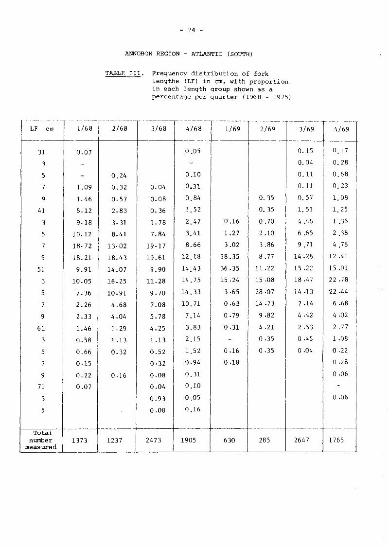
- 74 -
ANNOBON REGION - ATLANTIC (SOUTH)
TABLE III. Frequency distribution of fork lengths (LF) in cm, with proportion in each length group shown as a percentage per quarter (1968 - 1975)
LF cm
31
3
5
7
9
41
3
5
7
9
51
3
5
7
9
61
3
5
7
9
71
3
5
Total number
measured
1/68
0.07
-
-
1.09
1.46
6.12
9.18
10.12
18-72
18.21
9.91
10.05
7.36
2.26
2.33
1.46
0.58
0.66
0-15
0.22
0.07
1373
2/68
0.24
0.32
0-57
2.83
3-31
8.41
13-02
18.43
14.07
16.25
10-91
4.68
4.04
1.29
1.13
0.32
0.16
1237
3/68
0.04
0.08
0.36
1.78
7.84
19-17
19.61
9.90
11.28
9.70
7.08
5.78
4.25
1.13
0.52
0-32
0.08
0.04
0.93
0.08
2473
4/68
0.05
-
0.10
0.31
0.84
1.52
2.47
3.41
8.66
12.18
14.43
14.75
14.33
10.71
7.14
3.83
2.15
1.52
0.94
0.31
0.10
0.05
0.16
1905
1/69
0.16
1.27
3.02
38.35
36-35
15.24
3-65
0.63
0-79
0.31
-
0.16
0.18
630
2/69
0. 35
0. 35
0.70
2 .10
3.86
8.77
11.22
15-08
28-07
14.73
9-82
4-21
0-35
0-35
285
3/69
0.15
0.04
0.11
0. 11
0.57
1.51
4 .46
6 .65
9.71
14-28
15.22
18.47
14 .13
7 .14
4-42
2-53
0-45
0-04
2647
4/69
0.17
0.28
0.68
0.23
1.08
1.25
1.36
2 .38
4 .76
12 .41
15 .01
22 .78
22 .44
6 .68
4 -02
2.77
1 .08
0 .22
0-28
0,06
-
0.06
1765

- 75 -
TABLE 1 1 1 . !• <.nt-<l)
LF cm
31
3
•>
7
9
41
3
5
;
9
51
3
5
7
9
61
3
5
7
9
71
3
5
T o t a l nuntoer
measured
1/73
2-97
1 1 . 4 9
32-05
25-64
11-82
9 .50
4 -88
0 .84
0 . 7 0
0 . 0 8
0 . 0 3
3569
2 / 7 3
0 . 4 3
1.14
5. 12
5.85
7.46
HI.02
13-59
13-22
9-84
10-90
6-59
4 . 8 1
3 .28
2 .35
1.64
1.56
1.16
0 . 5 3
0 .26
0 .05
3781
3 /73
0 . 0 3
0 .24
0 .7 J
1.65
4 . 2 1
9 . 3 3
1 4 . 3 2
13-75
11-12
10 .18
10-48
6 . 9 1
9 . 0 6
4 . 5 1
1.48
1.18
0 . 74
0 . 1 0
2968
4 / 7 3
4.1 ' )
9 .1 ••'.
22 .94
25-55
17-45
11 -23
6 .16
0-47
0 . 5 0
0 . 9 7
0 . 4 7
0 .20
0 . 1 7
0 . 2 0
0 . 1 7
2986
1/74
0 .07
0 • 28
1-41
4 . 3 7
22-88
36-16
17-31
6 . 6 3
2-91
2 . 6 3
3 .52
1.09
0 . 4 6
0 . 2 0
0 .04
0 .02
5396
2/74
0 .44
0 . 8 5
1-11
7.2.6
1 2 . 4 2
24-11,
18-62
12.81
6-66
2 . 4 3
2 .92
2 . 1 8
2 . 5 1
1.53
0 . 9 3
0 .54
0 .22
0 .11
0 . 1 1
0 . 0 3
0 .19
3662
3/74
0 . 1 0
0 .4 7
2 .03
5 .53
9-32
15-20
19-57
17.66
13-19
6 .47
4 . 2 6
1.78
1.58
0 . 9 2
1.00
0 . 5 3
0 .12
0 .14
0 .14
0 .02
5119
4 /74
0 . 0 4
0 . 2 5
1 .40
3 .33
4 .92
9 . 0 1
13-97
13-92
15-00
1 2 . 2 3
8 . 8 3
8 .87
5 .88
1.17
0 .57
0 .21
0 . 1 2
0 .02
0 . 2 5
_
_
0 .02
_ . . : _ .
5648
1/75
0 . 2 5
1 .02
3.32
9 .72
1 5 . 6 8
19-80
12 .69
7 .55
7 . 8 5
11 .32
9 .04
1.15
0 .22
0 . 2 2
0 .16
-
-
-
_
-
_
3641
2 /75
0 .07
-
1 .88
4 .37
/ . 9 2
10.21
11-28
11 -55
10 .61
10 -48
9 .27
6 .58
2.3.5
2 .28
2 .41
2 .22
3 .09
2 .42
0.81
0 .20
-
"
1489
3/75
0 .08
0 . 2 8
0.54
0 .90
2 .28
6.1.1
1 0 . 9 6
15 .76
11-65
.12.37
12-42
9 .06
6 .85
3 .05
3 .00
2 . 0 8
1 .28
0 .72
0 .62
-
-
-
-
3897
4 / 7 5
0 .14
0 .19
1.28
2-94
7 .50
9 .94
1 5 - 8 3
1 7 . 1 5
13-00
8 .64
4 - 8 5
5.33
5 . 3 1
2 .53
1 .83
1 .13
0 . 5 5
0 . 4 3
0 . 7 0
0 . 5 5
0 . 0 7
-
0 . 0 7
4145

CAPE VERDE REGION - ATLANTIC (NORTH)
TABLE IV. Frequency distribution of fork lengths (LF) in Proportion in each length group shown as a per per quarter (1968 - 1975)
LF
cm
31
3
5
7
9
41
3
5
7
9
51
3
5
7
9
61
3
5
T o t a l Nb. 3f s k i p j a c k } m e a s u r e d
I
0 . 7 6
0 . 7 6
7 .85
2 3 . 2 9
3 4 . 6 8
26-08
6 . 5 8
395
1 9
I I
0 . 0 1
0 . 0 1
0 . 0 8
2 3 . 3 0
34 .67
26-02
0 . 0 7
1099
6 8
I I I
2 . 1 0
2 . 5 8
7 .40
19 .85
2 0 . 4 4
12 .26
9 . 1 5
7 .85
7 .32
7-32
2 .37
1.08
0 . 1 6
0-16
1859
II II II II II
iv !! i II h II H n II
0 . 1 0 || II
0 . 6 3 ||
3 .07 || II
6.13 1! jj
8 .66 || II
1 3 . 5 7 || 2 .14 j |
18 .10 1! 7 .49 ||
1 5 . 7 1 II 16 .04 |f
11 .72 || 1 8 . 1 8 ||
7.15 II 17.64 jj
3.35 II 14-97 II
4 - 8 6 II 1 5 - 5 0 II
3.70 II 5.35 ii
2.19 II 2.14 jj
0.92 II 0.53 II
0-10 Ii II II II II II II II II
2055 1! 187 II II II
1 9
11
2 . 2 7
7 . 5 3
16 .19
18 .04
1 7 . 6 1
1 4 . 7 7
15-76
5 . 1 1
1.99
0 . 4 3
0-14
0-14
704
6 9
I I I
2 . 0 4
2 . 5 2
7 . 3 9
1 9 . 8 1
2 0 . 4 4
1 2 . 2 6
9 . 1 2
7 .86
7 .39
7-39
2 . 3 6
1.10
0 . 1 6
0 - 16
636
iv 1!
0 . 0 6 ||
0 . 6 1 |!
3.05 1!
6 . 0 9 ||
8 . 6 4 ||
13.57 II
1 8 . 1 1 ||
1 5 . 7 3 ||
1 1 . 7 4 ||
7 . 15 ||
3 . 3 8 ||
4 -86 ||
2.22 Ii
0.94 I,
0.06 II
1805 ||
I
1 .85
6 .17
1 1 . 7 3
23 .46
1 7 . 2 8
7 .41
4 .32
7-41
5 .56
6 .17
5 .56
2 . 4 7
0-62
162
1 9
I I
0 . 0 9
1.52
3 .92
1 1 . 3 2
13 .64
1 5 . 2 4
15 .86
1 5 . 9 5
1 3 . 9 0
7-04
0 . 8 9
0 . 16
0 . 1 8
0 . 0 9
1121
7 0
I I I
0 . 2 6
1 .18
3 . 4 8
1 0 . 3 6
2 4 . 9 1
23 .86
11 .60
7 .02
4 . 9 8
6 .49
4-59
0 .59
1525
0
0
2
7
10
13
17
12
11
12
7
3
0
0
2

TABLE IV . ( con td )
LF
cm
31
3
5
7
9
41
3
5
7
9
51
3
5
7
9
61
3
5
T o t a l n b . o£ s k i p j a c k
measured
I
0 .34
2 .87
3.72
12 .16
1 3 . 5 1
15 .88
10-98
14 .19
1 3 . 0 1
10 .47
2 . 0 3
0 .84
592
1 9
I I
0 -13
0 . 2 7
1.35
4 . 7 1
8 .38
7-67
9-69
1 5 . 7 5
20-72
1 7 . 2 2
9 . 2 8
3 .63
0 .27
0 . 2 7
0 . 1 3
743
7 2
I I I
0 -40
0 . 9 8
4 . 8 8
2 . 8 4
1 4 . 9 6
23-22
0 . 0 9
1.95
19-49
3 .46
1 3 . 6 3
1 0 . 8 3
2 . 9 3
0 . 2 7
0 .04
2252
II II n II
iv i! H
II II II
II II
0.18 '!
2 .38 !!
6.68 J!
8.35 II
5-48 ||
8-68 I!
8.33 r
11-00 1
12.83 1
17.25 I
14.93 1
2.73 1
1.28 I
0.06 I i i
5089
I
4 . 2 0
11-89
13 .29
15-38
10 .49
16 .08
22 .38
6 . 2 9
143 i i i
1 9
I I
0 -05
0 . 3 6
0 . 4 1
1.94
4 . 5 1
10-20
15-43
14 .89
15 -83
12 .18
9 . 6 1
7 .85
3 .29
3 .02
0 . 4 1
2216
7 3
I I I
0 . 07
0 . 5 1
2 . 9 9
1 0 . 0 8
1 6 - 0 3
19-46
6 .49
8-06
1 0 . 4 9
1 1 . 5 6
1 0 . 7 0
3 .08
0 . 4 2
0 .07
4516
IV
0 . 5 0
0 . 7 5
3 .75
9 .04
16 .54
24-08
18-79
9-04
4 -00
4 . 5 0
6 .26
2 .50
0 . 2 5
3597
II II II II II II II II
II II II
n II
1! II H II II |i II II
1! II
II II
II ii II II || II II II II II II II II II II II II II II II II II II II II II II II II II II II 11 II II II II II II II
I
1 9
I I
0 . 1 4
1.28
7 . 4 1
1 2 . 1 3
31 .38
31-09
8-84
4 . 7 1
1-85
0 . 2 9
0 . 5 7
0 . 1 4
0 .14
701
0 .22
0 .74
2 .54
5-53
12-05
12 .57
19-86
24 .22
15 .74
5 .38
0 .92
0 .22
2713
7 4
I I I
0 . 1 6
0 . 4 5
2 . 1 6
5-47
11 -18
1 2 . 3 3
9-55
1 5 . 8 8
2 1 . 6 0
1 9 . 3 0
1 .60
0 . 2 0
0 .09
6930

- 78 -
Fork length
LF r70 - rv
-60
-50
-40
-30
-20
-10
• •
•
• •
1 1
•
1 .
•
•
1
O
1
0 o
o
READER A Untagged fish o Tagged fish 0
READER B •
l i I 100 200 300 400 500 600 700 800
Number of "daily" growth marks (Lewis, 1976)
Fig. 1 - Results of counting daily growth marks on the otoliths of skipjack in Papua New Guinea by two "readers".

Recapture p o i n t s of tagged skipjack tuna in Papua Mew Guinea 1972-1974 (from Lewis, 1

6
4
2-\
N Skipjack tagged betw (measured length)
n
AN I 2 3 4 5 6 7 8 9 10 II 12 13
T — ' — i — ' — i 1 —
i i 1 1 1 1 r
Skipjack tagged betw (measured length)
n
- i 1 1
0 I 2 3 4 5 6 7 6 9 10 II 12 13
Fig . 3 - Frequency d i s t r i b u t i o n s of annual increments A_l_ expressed in cm for sk At
in Papua New Guinea and at large for 5 to 12 months

- 81 -
% is
3
19
10
s
I *
IS
K>
8
rrThrp-tTl 11
%
Auqust 197 3 ,5
N 91b '0
u -Twrr| I
June N s 4 9 3 7
llTrt-m—,
-wrlflh>rTflTrTTin->.-r
September N ' 1433
^llnTflJiyn-,, -
Or:tobor N * 9 6 7
IS
10
5
l-*-*-* I "hffmiiiiw
"T"
November N * 1229
J Ufflmi
December X • 1832
£ * »
-*£ f l , mffltb^
J a n u a r y 1974 ,5
N » 2 7 7 9 10
F e b r u a r y 2 6 Kt
^jflh^iTthJ " IS
IO
s
March N = 2512
f T r T T T T H ^ - - ,
IS
10
s-
JIlllTtTTTW A p r i l
N • 2 6 4 8
.—<fflilnnjih^ May
H - 3919
IS-
10
-<-rrrrr| Itht^.
J u l y N ' 4 0 3 1
^fTfjl 111 IHTTT
— 1 — — I —
Auqust
N = 2671
41 I T T - ^ M -
September N » 4 4 9 2
41 October N * 4 6 S 4
r - W
Novembe r M ' 3883
lb
J December N • 4 8 9 6
! > » .
Oh,
January 1975 N * 245S
I F .
p . nJ-{ I I 11^ .
J i t i f i
F e b r u a r y N > 2 BOS
March N = 734
L F.
3 3 4 0 4 5 5 0 55 SO 6 3 70 55 4 0 4 5 50 S5 6 0
l n cm as ro
m cm
'iq. 4 - Monthly histoqrams of skipjack size frequencies - Nos 'be (Madaqascar) , Tndian Ocean. (Marcille and Stequert, 1976)

- 82 -
Juillvt 1976
40qn
*
*-- r±*- • » »-• • • i • .
SOcm '«J«m 'TOem SOcm
Aout 1976
a » •» i • * — ! • * • T , . • » . * I, ^ « *—1_J •_
Scptembre 1976
t •, f , » : — - i — L L i — • — • _ _t-J JJU-
Octobr* 1976
- * - . . _ i—>> i m i i ...>...i 1—
Novwnbre 1976
_i_ l—t-a- t—l t - l _
Mcwnbrt 1976
*
..+.1 l+l >
Jonvwr 1977
Fvvrwr 1977
I « I t 1 t !_•_
Mar* 1977
• » » • • *
Avril 1977
• j — . _ ! _ —*—•—*.—•_ •» « -
Mai 1977
_ l — 1 — L . S—f_ __l—I 1 t_
Jutn 1977
Juilltt 1977
Aout 1977
• l « *** , • f 1 • 1 «_
S#ptembr» 1977
- i — t m m i i i . • |
Oetobre 1977
X l.t ? ^ l — 1 J . U U 1 1 X -
*• *
Novwnbre 1977
0«c«mbrt 1977
Jonvier &/o
Fig. 5 - Points represent the modal values obtained for each landing sampled. Asterisks represent the position of the modal values obtained for the whole of the measurements made in one month.

- 8 3 -
6 0 c
x: •r-|
180
160
140
120
100
80
60
40
20
0 -»—I—•—I—i—I—>—I—•—I—i—I—i I i I • ' • i Srf. 10 12 14 16 18 20 ' 25 30
Age i n y e a r s
40 50 6 0
F i g . G r o w t h o f B e l g i a n s ( m e n ) . Thompson ( 1 9 4 8 )
B u c
c l-J
i oo r
90 _
80 _
70
60
50
40
30
20
10
_ l _ F i g . 7
1 2 3 4 5 Age i n y e a r s
Growth of cod.
Graham (19 33)