gruppe nr. 110 kurs: mo ws 2012 / 2013 - physik.leech.it nr. _____ kurs: mo ws 2012 / 2013 versuch:...

FAKULTÄT FÜR PHYSIK

PHYSIKALISCHES PRAKTIKUM FÜR FORTGESCHRITTENE

PRAKTIKUM MODERNE PHYSIK

Gruppe Nr. ________ Kurs: Mo WS 2012 / 2013

Versuch:________________________________________

Namen:_________________________________________

______________________________________________

Assistent: _______________________________________

durchgeführt am:___________________________________

Protokollabgabe am:_________________________________

____________________________________

Note gesamt

Datum:_________________

anerkannt:____________________________

Bemerkung:

+ - 0

110

Positronium

Fleig, Georg

Krause, Marcel

Porcelli, Alessio

07.01.13

Physikalisches FortgeschrittenenpraktikumP3

Experiment:

Mean lifetime of positronium

from the subarea

Nuclear Physics

Lab report

of

Georg Fleig ([email protected])

Marcel Krause ([email protected])

Group:110

Date of experimental execution:

07.01.13

mailto:[email protected]

mailto:[email protected]

I. Preliminary

AbstractAim of the present work is the measurement of the mean lifetime of positronium by recording energy

spectra of the positronium source 22-Na. In addition, we will measure the speed of light.

Theoretical background

AnnihilationThe process of annihilation is observed whenever an elementary particle collides with its antiparticle.

The conservation of momentum and energy indicates that the annihilation of any pair of particles and

their antiparticles must create at least one new particle.

e+ e 2 e+ e 3

Figure 1: Feynman diagrams of electron-positron annihilation (source: [1]).

Let the particles be a pair of an electron and a positron. The collision annihilates both of them, thus

creating a new particle, namely a photon. It is also possiblethat not only one, but two, three or even

more photons are created, as it is shown in the Feynman diagrams in figure 1. Let the momentum of

both the electron and the positron be zero at the time of the annihilation. Due to the conservation of

momentum and energy and the fact that photons can never rest,it is obvious that the creation of one

single photon can only take place in solid-state bodies which are able to take the inverse momentum of

the created photon.

The second possible form of decay is that the electron-positron pair decays into two photons whose

momenta are opposed. The conservation of energy predicts that every of the two photons has an energy

of approximately511 keV which matches the rest mass of an electron.

The third form of decay is the annihilation into three photons. Due to the laws of conservation, these

photons can have arbitrary energies and momenta. In the following, we want to neglect the annihilation

into one single photon because of its low cross section and therefore low probability of taking place.

Let us now additionally have a look at the spins of the two particles. It should be mentioned that we

can neglect the orbital angular momenta completely becauseof the fact that they are very low compared

to the spins in solid-state bodies. By adding two particles with spin 1/2 one can analytically show that

there exists one eigenstate for the overall spinS = 0 and three different eigenstates forS = 1, therefore

calling them singlet and triplet state, respectively.

Photons are gauge bosons with a spin of 1. Two photons moving in opposed directions can therefore add

4

to an overall spin of either 0 or 2. However, three photons moving in arbitrary directions have a chance

of adding their spins to an overall spin of 1. Thus, the singlet state can only decay into two photons and

the triplet state into at least three, which means that the decay of the triplet state is a process of higher

order, making it less probable than the decay of the singlet state. Let us have a look at the cross sections

of both forms of annihilation

σ2γ = απ~

v, σ3γ = α2 3π~

8v(1)

whereα ≈ 1/137 is the fine-structure constant andv ≪ c the relative velocity of the particles. The ratio

of both cross sections is as follows:σ3γσ2γ

≈1

372(2)

Consequently, in free space we want to neglect the decay of the triplet state and only consider the singlet

state in the following.

Generation of positroniumInstead of one electrone− and one positrone+ annihilating each other, it is possible that both can form

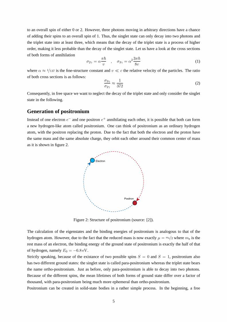
a new hydrogen-like atom called positronium. One can think of positronium as an ordinary hydrogen

atom, with the positron replacing the proton. Due to the factthat both the electron and the proton have

the same mass and the same absolute charge, they orbit each other around their common center of mass

as it is shown in figure 2.

Electron

Positron

Figure 2: Structure of positronium (source: [2]).

The calculation of the eigenstates and the binding energiesof positronium is analogous to that of the

hydrogen atom. However, due to the fact that the reduced massis now exactlyµ = me/2 whereme is the

rest mass of an electron, the binding energy of the ground state of positronium is exactly the half of that

of hydrogen, namelyE0 = −6.8 eV.

Strictly speaking, because of the existance of two possiblespinsS = 0 andS = 1, positronium also

has two different ground states: the singlet state is calledpara-positronium whereas the triplet state bears

the name ortho-positronium. Just as before, only para-positronium is able to decay into two photons.

Because of the different spins, the mean lifetimes of both forms of ground state differ over a factor of

thousand, with para-positronium being much more ephemeralthan ortho-positronium.

Positronium can be created in solid-state bodies in a rathersimple process. In the beginning, a free

5

positron travels through the body. As a result of its high velocity, its kinetic energy is too high to either

create positronium or to annihilate with a effectively freeelectron of the solid body. Instead, the velocity

of the positron is reduced by numerous inelastic collisionswith the atoms of the solid-state body until its

kinetic energy is within the range of a feweV.

As a result of the inelastic collisions, the atoms have a chance of being ionised. The positron can now

either combine or annihilate with the free electron of the ionised atom. There exists a certain range∆E

of energy for the positron where only the building of positronium but no other type of inelastic collision

is possible. The limits of this range is the ionisation energy V minus the binding energy of positronium

(due to its creation) as a minimal energy on one side and the first stimulation energyEa of the atoms on

the other side. This certain energy range is often called theOre gap:

∆E = Emax−min = Ea − (V − 6.8 eV) (3)

Positronium in solid-state bodiesThe question arises how the existence of positronium can be proven. One could try to detect the annhilia-

tion of positronium and therefore the creation of two or three gamma quanta. However, it is also possible

that these quanta originate from the annihilation of a free electron-positron pair. Thus, it is necessary to

consider another way of positronium detection.

When building the ratio of the two possible forms of decay, one basically builds the ratio between the

two cross sections. For a free electron-positron pair the result is given in equation (2). However, during

the creation of positronium the triplet state has a three times higher chance of being built than the singlet

state, which stems from the fact that the triplet state consists of three different eigenstates. Therefore, the

ratio for the creation becomes:σ3γσ2γ

=3/41/4

= 3 (4)

In reality, the ratio is lower than given in (4) because of interaction between the rather long-living ortho-

positronium and the solid-state body. When measuring positronium in a solid-state body like a polymer,

three different components are found.

The first is a rather long-living component with a mean lifetime of2 ns - 4 ns making up around 30%

of all annihilations. It belongs to ortho-positronium. Thesecond component is the most intense with

an annihilation ratio of approximately 60% and a mean lifetime of 0.5 ns. It stems from the decay of

free electron-positron pairs. The last component with a mean lifetime of approximately0.12 ns is the

shortest-living and with 10% of all annihilations the leastintense one. It belongs to para-positronium.

The difference of the mean lifetimes of ortho-positronium in a solid-state body compared to a positron-

ium atom in free space is remarkable. Basically, this difference is explained with two processes in the

solid body, the first being so-called pick-off processes.

Ortho-positronium interacts with electrons from the molecules of the solid body or their inner magnetic

fields. With the ortho-positronium now having an impact partner, the solid body can take up energy and

angular momentum of the triplet state. Therefore, it is possible that even the triplet state can decay only

into two photons instead of at least three. This increases the chance of the triplet decay considerably.

The energy of the created photons are continuously distributed up to maximum of511 keV.

The second possible interaction is the conversion between ortho-positronium and para-positronium made

6

possible by interchanging electrons from the positronium and from molecules of the solid body. The con-

version can happen in both directions with the same probability. However, the probability of decay of

the singlet state is higher and that of the triplet state is lower than the conversion probability, thus the

conversion causes a higher rate of annihilation than one of creation of ortho-positronium. Due to the

conservation of energy and angular momentum, the conversion process leads to the creation of photons

with a fixed energy of511 keV.

Overall, the reduction of the mean lifetimeτortho of ortho-positronium due to pick-off processesτp and

conversionτc is given by1

τortho=

1

τ0+

1

τp+

1

τc(5)

whereτ0 is the mean lifetime of undisturbed ortho-positronium without any interaction.

Source of 22NaIn order to induce the creation of positronium in e.g. polymers, free positrons have to be created. One

way of achieving this is theβ+ decay

p → n+ e+ + νe (6)

where a protonp in a nucleus decays into a neutronn, a positrone+ and an electron neutrinoνe. This

reaction is always possible if the resulting nucleus has a greater binding energy than the original one.

However, it is not easily possible to detect the exact time ofcreation of the positron during theβ+ decay

in general.

In order to solve this problem,22Na is used as a source of positrons. Itsβ+ decay is as follows:

22Na→ 22Na∗ + e+ → 22Na+ γ + e+ (7)

The whole reaction takes place within a very small time span,therefore the creation of the positron and

a gamma quantumγ with an energy ofEγ = 1.275MeV is effectively synchronous. Due to the fact that

the time needed to decelerate this gamma quantum in solid bodies is almost the same as the time needed

for the positronium to slow down to reach the Ore gap, the gamma quantum may serve as some kind of

stopwatch.

Exercise 0: Experimental set-upTheβ+ source, namely22Na, is enclosed by acrylic glass and lies between two movabledetectors po-

sitioned in an angle of 180◦. One detector registers the gamma quantum of the22Na source, giving a

start signal. The other detector shall be moved in order to allow measurements at different distances.

It registers the whole spectrum of the source as well as the spectrum of all processes happening in the

acrylic glass.

In order to process the data, the two detectors are connectedwith a computer.

7

Exercise 1: Time calibration and time resolutionThe time pulse converter (TPC) is only working correctly if there is a certain time span between start and

stop of at least∆t = 2ns. Because of the fact that the TPC is only able to display events per channel

number but not per time as it is needed during the experiment,we have to calibrate it. We will detect a

whole spectrum of22Na and afterwards only the positronium decay with differentdelay times∆t. The

peak of the positronium decay can be approximated as a Gaussian bell curve with its maximum at a

certain channel number.

By increasing the delay time, we also move the maxima to higher channel numbers. When plotting the

delay time over the channel number, we expect to see a linear relationship between those two values.

With the help of a linear fit, we are then able to calibrate the TPC. The time resolution is then given as

the product of the full width at half minimum (FWHM) of the bell curve with the delay time per channel.

Exercise 2: Mean lifetime of positroniumIn order to measure the mean lifetimes of the different positronium states we will record another spec-

trum. Due to the fact that we calibrated the TPC before, we cannow change thex-axis from channel

numbers to time. Because of the limited time resolution it will not be possible to differ between the two

short-living states of para-positronium on one hand and theannihilation between free electron-positron

pairs in the acrylic glass on the other. Therefore, the spectrum will be of the form

N(t) = A exp

(

−t

τ1

)

+B exp

(

−t

τ2

)

+ C (8)

with the constantsA, B andC and theτi being the mean lifetimes of long-living and generally short-

living positronium respectively. With the help of appropriate fits it is possible to determine the lifetimes.

In order to get rid of the random coincidencesC we will consider large times where the exponential con-

tributations of the positronium have vanished. Afterwards, we are able to subtractC from the spectrum.

Exercise 3: Speed of lightFinally, we also want to measure the speed of light with the help of theβ+ source. In order to achieve

this, we will record the positronium decay at two different distances between the detector and the source.

The maxima of the two spectra will then also be found at different times. We can immediately calculate

the speed of light by building the ratio of these values.

References[1] Blaues Buch zur Kernphysik

[2] http://en.wikipedia.org/wiki/File:Positronium.svg

8

http://en.wikipedia.org/wiki/File:Positronium.svg

II. Results and Discussion

Exercise 1: Time calibration and time resolutionFirst of all, we fixed the vial out of acrylic glass, which contained the22Na, between the two detectors.

The movable detector was fixed at a position of zero from the22Na, meaning that it reached its minimum

distance from it. We set the manual delay of the TPC to a time of∆t = 2ns and started the first

measurement. On the computer, we were able to see a plot of thenumber of events over the channel

number of the TPC as it is shown in figure 3.

0 200 400

0

1000

2000

Num

ber o

f eve

nts

Channel number

Figure 3: Full spectrum of22Na.

On the spectrum, we are able to see a few characteristic peaks, with the most interesting one around

channel number 100. The high number of events in the channelsbelow mostly stem from the free

positron-electron annihilation, which is not interestingfor measuring the mean lifetime of positronium.

Therefore, we increased the lower level of the trigger in order to neglect all events from low channels.

The resulting spectrum is shown in figure 4.

10

0 200 400 600

0

200

400N

umbe

r of e

vent

s

Channel number

Figure 4: Reduced spectrum of22Na.

In the chart, the expected peaks can be seen. The huge peak from the decay of the positronium belonging

to an energy of approximately511 keV that can be seen in figure 3 is now cut off in figure 4. The other

peaks that are actually visible in figure 4 are the gamma quanta γ originating from equation (7).

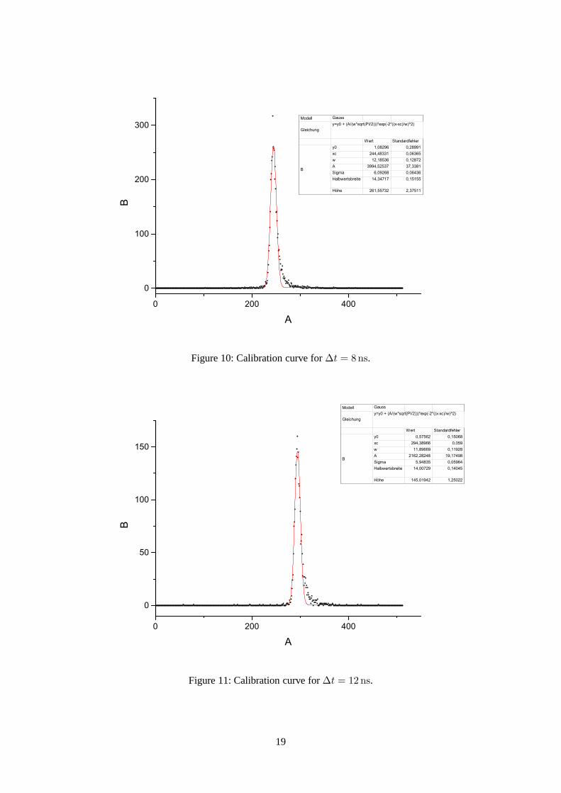
In order to calibrate the TPC, we used the signals we obtainedfrom both the decay and the gamma

quantum as triggers. In the following, we measured the number of events for different manual delay

times, where the delay time∆t = 2ns should be our zero value. The resulting figures 8 to 13 are shown

in the appendix. With the help of Origin, we fitted Gaussian bell curves of the form

N = N0 +A

σ√

π/2exp

(

−2(x− xc)

2

σ2

)

(9)

into each chart in order to find the maximum channel numberxc of the distribution. The results are

shown in table 1, withσxcbeing the standard deviation given by Origin.

∆t in ns 0 4 8 12 16 20

xc 145.314 193.657 244.483 294.390 346.103 392.634σxc

0.050 0.059 0.064 0.059 0.060 0.058

Table 1: Maximum channel numbers against delay times

Plotting the delay time against the maximum channel numbers, we are able to linearly fit the data with a

11

function of the form

t = mx+ t0 (10)

as shown in figure 5. The required parametersm and t0 with their standard deviations for the axis

transformation from channel numbersx to timest are printed in table 2. With respect to them, we get:

t = (0.080 ± 0.005) ns · x− (11.627 ± 1.355) ns . (11)

Note that the errors of the channel numbers from the Gaussianfit are very small compared to the respec-

tive channel. Therefore, the error bars in figure 5 may not be misinterpreted as error bars with respect to

the time, but rather as such with respect to the channel numbers.

100 200 300 400-4

0

4

8

12

16

20

Del

ay ti

me

[ns]

Channel number

Gleichung y = a + b*x

Wert Standardfehler

BSchnittpunkt mit der Y-Achse

-11,62707 1,35552

Steigung 0,08027 0,0048

Figure 5: Time calibration.

m in ns σm in ns t0 in ns σt0 in ns0.080 0.005 -11.627 1.355

Table 2: Calibration parameters.

Now that the time calibration is done, we are able to determine the time resolution of the TPC. The needed

full widths at half maximum (FWHM) and their respective errors given in the charts in the appendix and

abstracted in table 3. With regard to the fact that the time resolutionδt is given as the product of FWHM

12

and the time per channel numberm, we can calculate it as follows:

δt = FWHM ·m (12)

The result of these calculations are also shown in table 3.

∆t 0 4 8 12 16 20

FWHM 14.944 14.658 14.347 14.007 13.711 13.983σFWHM 0.119 0.141 0.152 0.141 0.143 0.138

δt 1.196 1.173 1.148 1.121 1.097 1.119σδt 0.063 0.063 0.063 0.063 0.063 0.063

Table 3: Determination of the time resolution.

The errorsσδt in δt were calculated with the Gaussian error propagation:

σδt =

√

(

∂δt

∂mσm

)2

+

(

∂δt

∂FWHMσFWHM

)2

= |δt|

√

(σm

m

)2

+( σFWHM

FWHM

)2

.

(13)

Building the average of all the time resolutions, we finally get:

δt = (1.142 ± 0.063) ns (14)

It should be noted that the time resolution is remarkably higher than the error we got in the calibration

parameterm. Consequently, we want to neglect the errorσm and only regard a common errorσt0 for

every timet.

With the time calibration being done, we can now transform the channel numbers into times for every

following exercise. By doing so, we want to neglect times below zero.

Exercise 2: Mean lifetime of positroniumAfter calibrating the TPC, we are now able to determine the mean lifetime of positronium. The mea-

surement shown in figure 8 was very precise, therefore, we decided to use the data again to obtain the

lifetimes. First, we transformed the x-axis from channel numbers to times according to equation (11). In

addition, we neglected any times below zero.

13

0 5 10 15 20 25 300

500

1000

1500N(t)

Time [ns]

Modell ExpDec2

Gleichungy = A1*exp(-x/t1) + A2*exp(-x/t2) + y0

Chi-Quadr Reduziert

87,83006

Kor. R-Quadrat 0,99617Wert Standardfehler

B

y0 0,87205 0,61706A1 1499,81631 33,20733t1 0,62812 0,01446A2 16,31195 35,8038t2 2,09752 2,55826k1 1,59206 0,03666k2 0,47675 0,58148tau1 0,43538 0,01003tau2 1,45389 1,77325

Figure 6: Double exponential fit.

Afterwards, we fitted the function (8) to our data. All the parameters as well as the data and the fit are

printed in figure 6 and the important parameters concerning the lifetime are sumarized in table 4.

τ1 in ns στ1 in ns τ2 in ns στ2 in ns0.628 0.015 2.098 2.558

Table 4: Mean lifetimes of positronium

The errors shown in the table above stem directly from the conversion of the x-axis from channel numbers

to times. The errors in equation (11) serve as weights for thedouble exponential fit, therefore we do not

have to consider the error propagation here. Thus, the mean lifetimes of positronium are:

τpara, free= τ1 = (0.628 ± 0.015) ns

τortho = τ2 = (2.098 ± 2.558) ns(15)

Both para-positronium and the free positron-electron annihilation share the same measured value because

the detectors are not precise enough to separate them from each other. Comparing these to the literature

valuesτpara,lit = 0.12 ns, τfree,lit = 0.5 ns andτortho,lit = 2ns− 4 ns we see that our results are within the

expected range. The biggest source of error is most likely the precision of the used detectors. As we have

seen before, the time resolution is relatively high, therefore we can not expect very precise measurements

with respect to the mean lifetimes.

14

Exercise 3: Speed of lightIn the end, we performed further measurements in order to calculate the speed of light. As described

in the preliminary, we recorded the spectra at four different distancesd between the start and the stop

photomultiplier. Increasing the distance resulted in lower event rates and a shift of the signal peak

towards higher channel numbers. Again, with the help of the time calibration in equation (11), we were

able to transform the channel numbers on the x-axis to times.The recorded plots can be found in graph

14 to 17 in the appendix. To determine the time of the peak we fitted Gaussian bell curves of the form

(9) into the charts. The error of time calibration has already been included in the charts and was regarded

by the applied fit. The results and the corresponding errorsσt are listed in table 5.

d in cm t in ns σt in ns

0 -0.00193 0.003997.5 0.00911 0.0048115 0.31985 0.0044220 0.55314 0.00422

Table 5: Position of the peaks at different distances.

Since we know now the distance and the time needed to travel this distance, we can directly calculate the

speed of light by applying a linear fit of the form

c = mx+ c0 (16)

to the data. Besides the error for the time, we also assumed a systematical error∆d = 0.5mm for the

distanced between the two photomultipliers. Both errors are added to chart 7 and respected by the linear

fit performed by Origin.

0,0 0,2 0,4 0,6

0

10

20

Dis

tanc

e [c

m]

Time [ns]

Gleichung y = a + b*x

Gewichtung instrumental

Fehler der Summe der Quadrate

11275,26965

Pearson R 0,93663Kor. R-Quadrat 0,81591

Wert Standardfehler

DistanceSchnittpunkt mit der Y-Achse

3,88364 2,58888

Steigung 30,63665 8,10257

Figure 7: Linear fit for determining the speed of light.

15

As the slope of the straight line is linked to the speed of light, we finally get

c = (3.06 ± 0.81) · 108m

s(17)

as a value for the speed of light. Compared to the literature valueclit = 3.00 · 108 m/s we only have a

small relative error of 2.0%. Despite this presentable value, our result is not that satisfying since the error

range is huge and the data points do not seem to follow a lineardistribution. Again, the main error seems

to stem from the high time resolution of the detector with respect to the small time differences measured

in this procedure. Another factor could be the increased measurement time for longer distances since

other disturbing signals have more time to reach the detector.

16

III. Appendix

0 200 400

0

500

1000

1500

Num

ber o

f eve

nts

Channel number

Modell Gauss

Gleichungy=y0 + (A/(w*sqrt(PI/2)))*exp(-2*((x-xc)/w)^2)

Wert Standardfehler

B

y0 4,79366 1,09585xc 145,31338 0,04984w 12,69256 0,10084A 20470,64792 144,04375Sigma 6,34628 0,05042Halbwertsbreite 14,94435 0,11873

Höhe 1286,83329 8,78568

Figure 8: Calibration curve for∆t = 0ns.

0 200 400

0

100

200

300

B

A

Modell Gauss


Wert Standardfehler

B


Höhe 217,96198 1,79802


18

0 200 400

0

100

200

300B

A

Modell Gauss


Wert Standardfehler

B


Höhe 261,55732 2,37511


0 200 400

0

50

100

150

B

A

Modell Gauss


Wert Standardfehler

B


Höhe 145,01942 1,25022


19

0 200 400

0

200

400

B

A

Modell Gauss


Wert Standardfehler

B


Höhe 330,61571 2,96181


0 200 400

0

200

400

B

A

Modell Gauss


Wert Standardfehler

B


Höhe 335,87145 2,85921


20

-4 -2 0 2 4

0

500

1000

1500

Num

ber o

f Eve

nts

Time [ns]

Modell Gauss


Chi-Quadr Reduziert

574,33118


Number of Events

y0 4,79366 1,09585xc -0,00193 0,00399w 1,01541 0,00807A 1637,65183 11,5235Sigma 0,5077 0,00403Halbwertsbreite 1,19555 0,0095Höhe 1286,83329 8,78568

Figure 14:d = 0cm.

-4 -2 0 2 4

0

100

200

300

Num

ber o

f Eve

nts

Time [ns]

Modell Gauss


Chi-Quadr Reduziert

26,61434


Number of Events

y0 0,71575 0,23514xc 0,00911 0,00481w 0,92195 0,00973A 252,68284 2,35607Sigma 0,46097 0,00486Halbwertsbreite 1,08551 0,01145Höhe 218,68021 1,98405

Figure 15:d = 7.5 cm.

21

-4 -2 0 2 4

0

100

200

300

Num

ber o

f Eve

nts

Time [ns]

Modell Gauss


Chi-Quadr Reduziert

23,92171


No of Events


Figure 16:d = 15 cm.

-4 -2 0 2 4

0

100

200

300

Num

ber o

f Eve

nts

Time [ns]

Modell Gauss


Chi-Quadr Reduziert

36,97793


Number of Events


Figure 17:d = 20 cm.

22

gruppe nr. 110 kurs: mo ws 2012 / 2013 - physik.leech.it nr. _____ kurs: mo ws 2012 / 2013 versuch:...

Documents