guatemala: selected issues and analytical notes; imf ... · environment, high red tape and...
TRANSCRIPT

GUATEMALA SELECTED ISSUES AND ANALYTICAL NOTES
Approved By Nigel Chalk
Prepared By Yixi Deng, Valentina Flamini, Jaume Puig-Forné,
Anna Ivanova, Carlos Janada, Rodrigo Mariscal Paredes,
Iulia Ruxandra Teodoru, José Pablo Valdés, Victoria Valente,
Joyce Wong (all WHD), Marina Mendez Tavares, Adrian
Peralta-Alva and Xuan Tam (SPR), Keiko Honjo and Benjamin
Hunt (RES), and Noelia Camara (BBVA), with editorial support
from Misael Galdamez and Patricia Delgado.
SELECTED REAL SECTOR ISSUES ________________________________________________________ 5
A. Potential Growth and the Output Gap _________________________________________________ 5
B. Food Inflation in Guatemala ___________________________________________________________ 9
C. Female Labor Force Participation in Guatemala _______________________________________ 15
References_______________________________________________________________________________ 21
FIGURES
1. Investment, Innovation, and Capital ____________________________________________________ 8
2. Guatemala and CAPDR: Inflation and Contributions to Inflation ______________________ 10
3. Food Prices ___________________________________________________________________________ 11
4. Drivers of Food Inflation ______________________________________________________________ 12
5. Remittances and Share of Food by Household Quintiles ______________________________ 12
6. Share of Rural Population and Trade Margins _________________________________________ 13
7. CAPDR: Employment Indicators _______________________________________________________ 16
8. Labor Force Participation Rates _______________________________________________________ 17
9. Female Labor Force Participation Rates _______________________________________________ 18
10. Gender Gap in Guatemala ___________________________________________________________ 19
TABLES
1. Potential Output Growth and Output Gap Estimates ___________________________________ 5
2. Regression Results Using Microdata __________________________________________________ 20
CONTENTS
August 2, 2016

GUATEMALA
2 INTERNATIONAL MONETARY FUND
APPENDIX
Multivariate Filter Methodology _________________________________________________________ 22
FISCAL POLICY: SUSTAINABILITY AND SOCIAL OBJECTIVES _________________________ 25
A. Fiscal Sustainability Assessment ______________________________________________________ 25
B. Poverty, Inequality and Fiscal Redistribution __________________________________________ 31
References_______________________________________________________________________________ 40
BOX
1. General Structure of the Model _______________________________________________________ 37
FIGURES
1. Fiscal Indicators _______________________________________________________________________ 25
2. General Government Debt Indicators _________________________________________________ 26
3. Long-Term Sustainability______________________________________________________________ 28
4. Alternative Scenarios __________________________________________________________________ 29
5. Public DSA – Stress Tests______________________________________________________________ 30
6. Evolution of Predictive Densities of Gross Nominal Public Debt _______________________ 30
7. Poverty and Inequality Indicators _____________________________________________________ 32
8. Revenue, Expenditure, and Social Spending ___________________________________________ 33
9. Consumption Distribution ____________________________________________________________ 33
10. Poverty Gap by Income Deciles ______________________________________________________ 34
11. Impact of VAT and PIT Increases on Economic Activity, Poverty, and Inequality _____ 37
12. Impact of Spending Alternatives on Economic Activity, Poverty, and Inequality _____ 38
APPENDIX
Model Details ___________________________________________________________________________ 41
MONETARY POLICY MANAGEMENT __________________________________________________ 46
A. Estimation of the Neutral Policy Rate _________________________________________________ 46
B. Monetary Policy in the Current Global Environment __________________________________ 50
FIGURES
1. Results: Cost-Push Shock (Positive) ___________________________________________________ 53
2. Results: Domestic Demand Shock (Negative) _________________________________________ 53
3. Results: Foreign Demand (Negative) __________________________________________________ 53
4. Results: Oil Price Shock (Positive) _____________________________________________________ 54
5. Foreign Interest Rate Shock (Positive) _________________________________________________ 54
6. Exchange Rate Shock (Negative/Depreciation) ________________________________________ 54

GUATEMALA
INTERNATIONAL MONETARY FUND 3
TABLE
1. Neutral Real Interest Rate for Guatemala _____________________________________________ 47
MACRO FINANCIAL LINKAGES: ASSESSING FINANCIAL RISKS ______________________ 55
A. Stress Testing the Financial System ___________________________________________________ 55
B. Domestic Bank Network Analysis and Cross-Border Financial Spillovers ______________ 64
C. Balance Sheet Analysis ________________________________________________________________ 70
D. Dynamic Macro Financial Linkages ___________________________________________________ 73
References_______________________________________________________________________________ 78
FIGURES
1. Network Analysis Based on Interbank Exposures ______________________________________ 65
2. Interbank Exposures __________________________________________________________________ 65
3. Bank Capital___________________________________________________________________________ 66
4. Capital Impairment____________________________________________________________________ 66
5. Index of Contagion and Vulnerability _________________________________________________ 67
6. Domino Effect and Contagion Path ___________________________________________________ 67
7. Foreign Bank Claims __________________________________________________________________ 70
8. Net External FDI and Debt Positions __________________________________________________ 71
9. Bank Credit ___________________________________________________________________________ 71
10. FSGM Model Simulations of Macro Financial Linkages ______________________________ 76
TABLES
1. Financial Soundness Heat Map _______________________________________________________ 57
2. Satellite Model for Credit Risk Dependent Variable:
NPL Ratio (Logistic Transformation) _______________________________________________ 58
3. Banking Sector Financial Soundness Indicators _______________________________________ 62
4. Results of Stress Tests _________________________________________________________________ 63
5. Spillovers from International Banks' Exposures ________________________________________ 69
6. External and Foreign Currency Positions ______________________________________________ 73
ANNEX
I. Net Intersectoral Asset and Liability Positions _________________________________________ 79
MACRO FINANCIAL LINKAGES: FINANCIAL DEVELOPMENT AND INCLUSION _____ 81
A. Financial Development in Guatemala _________________________________________________ 81
B. Financial Inclusion in Guatemala ______________________________________________________ 85
References_______________________________________________________________________________ 96

GUATEMALA
4 INTERNATIONAL MONETARY FUND
FIGURES
1. Financial Sector Development ________________________________________________________ 82
2. Financial Development Gaps __________________________________________________________ 82
3. Financial Institutions and Market Development, and Economic Growth _______________ 84
4. Physical Access to Financial Infrastructure and Enabling Environment ________________ 87
5. Use of Financial Services by Households and Firms ___________________________________ 88
6. Country-Specific Financial Constraints ________________________________________________ 92
7. Impact of Reducing Financial Constraints on GDP and Inequality _____________________ 93
TABLES
1. Financial Inclusion and Fundamentals _________________________________________________ 94
2. Determinants of the Financial Inclusion Gaps _________________________________________ 95
3. Characteristics of Financially-Included Population ____________________________________ 95
APPENDICES
1. Measuring Financial Development ____________________________________________________ 97
2. Construction of the Financial Inclusion Index ________________________________________ 101
3. Model Calibration ____________________________________________________________________ 105
GUATEMALA
INTERNATIONAL MONETARY FUND 5
SELECTED REAL SECTOR ISSUES
A. Potential Growth and the Output Gap1
This section estimates potential output growth and the output gap for Guatemala.
Potential output growth averaged at 4.4 percent just before the global financial crisis but
has declined since to 3¾ percent due to the lower capital accumulation and TFP growth.
It is estimated at 3.8 percent in 2016, and the output gap is virtually closed. Looking
forward, potential growth is expected to reach 4 percent in the medium-term due to the
expected improvements in TFP growth.
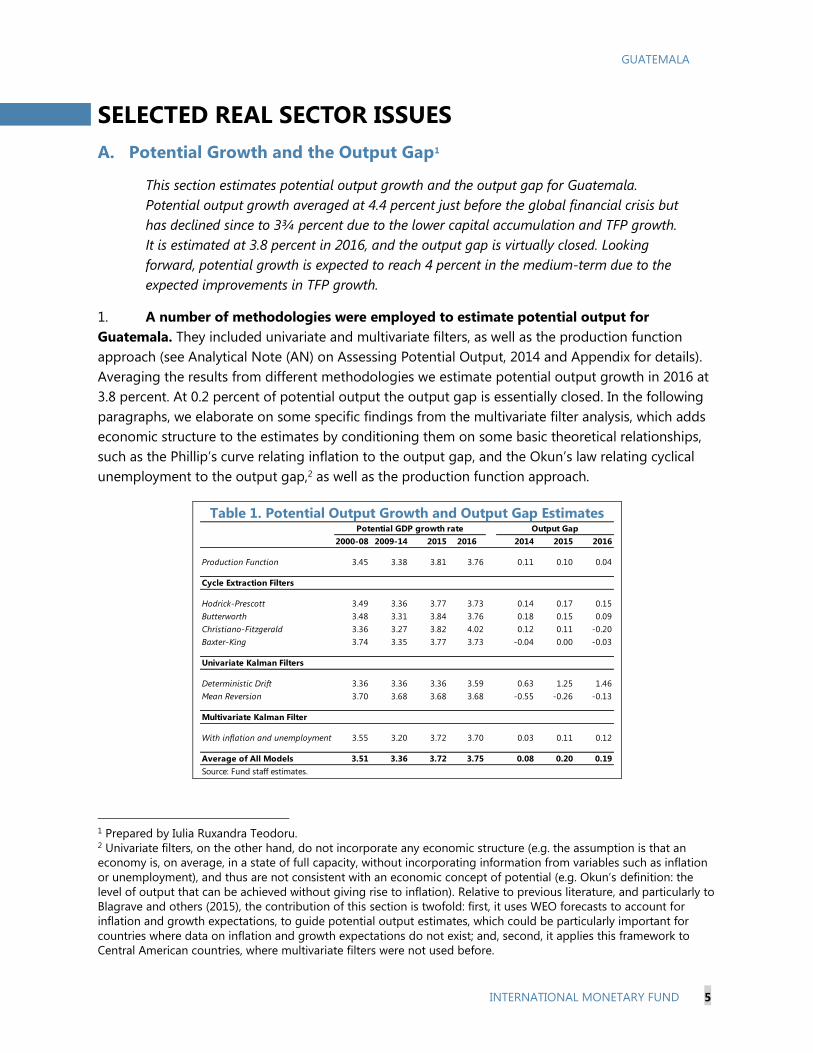
1. A number of methodologies were employed to estimate potential output for
Guatemala. They included univariate and multivariate filters, as well as the production function
approach (see Analytical Note (AN) on Assessing Potential Output, 2014 and Appendix for details).
Averaging the results from different methodologies we estimate potential output growth in 2016 at
3.8 percent. At 0.2 percent of potential output the output gap is essentially closed. In the following
paragraphs, we elaborate on some specific findings from the multivariate filter analysis, which adds
economic structure to the estimates by conditioning them on some basic theoretical relationships,
such as the Phillip’s curve relating inflation to the output gap, and the Okun’s law relating cyclical
unemployment to the output gap,2 as well as the production function approach.
Table 1. Potential Output Growth and Output Gap Estimates
1 Prepared by Iulia Ruxandra Teodoru. 2 Univariate filters, on the other hand, do not incorporate any economic structure (e.g. the assumption is that an
economy is, on average, in a state of full capacity, without incorporating information from variables such as inflation
or unemployment), and thus are not consistent with an economic concept of potential (e.g. Okun’s definition: the
level of output that can be achieved without giving rise to inflation). Relative to previous literature, and particularly to
Blagrave and others (2015), the contribution of this section is twofold: first, it uses WEO forecasts to account for
inflation and growth expectations, to guide potential output estimates, which could be particularly important for
countries where data on inflation and growth expectations do not exist; and, second, it applies this framework to
Central American countries, where multivariate filters were not used before.
2000-08 2009-14 2015 2016 2014 2015 2016
Production Function 3.45 3.38 3.81 3.76 0.11 0.10 0.04
Cycle Extraction Filters
Hodrick-Prescott 3.49 3.36 3.77 3.73 0.14 0.17 0.15
Butterworth 3.48 3.31 3.84 3.76 0.18 0.15 0.09
Christiano-Fitzgerald 3.36 3.27 3.82 4.02 0.12 0.11 -0.20
Baxter-King 3.74 3.35 3.77 3.73 -0.04 0.00 -0.03
Univariate Kalman Filters
Deterministic Drift 3.36 3.36 3.36 3.59 0.63 1.25 1.46
Mean Reversion 3.70 3.68 3.68 3.68 -0.55 -0.26 -0.13
Multivariate Kalman Filter
With inflation and unemployment 3.55 3.20 3.72 3.70 0.03 0.11 0.12
Average of All Models 3.51 3.36 3.72 3.75 0.08 0.20 0.19
Source: Fund staff estimates.
Potential GDP growth rate Output Gap
GUATEMALA
6 INTERNATIONAL MONETARY FUND
2. Potential growth increased from 3.3 percent to 4.4 percent from early to the mid-
2000s. The increase was driven by higher employment growth and less negative TFP growth.
Compared to other Central American economies such as Costa Rica, the Dominican Republic, and
Panama where an acceleration in TFP growth lifted potential growth by at least 2 percentage points
and as high as 5 percentage points in the case of Panama, the increase in Guatemala was small.
3. Potential growth declined from 4.4 percent in 2006–07 to 3.7 percent after the crisis in
2013–14. Lower capital accumulation and productivity growth explain the decline in Guatemala’s
potential growth during this period. Most other Central American economies also experienced
declines in their potential growth during that period on the account of lower capital accumulation,
employment, and TFP growth: by about 2 percentage points in Costa Rica, the Dominican Republic,
and Honduras and by about 1 percentage point in El Salvador and Panama. Potential growth
increased slightly only in Nicaragua.
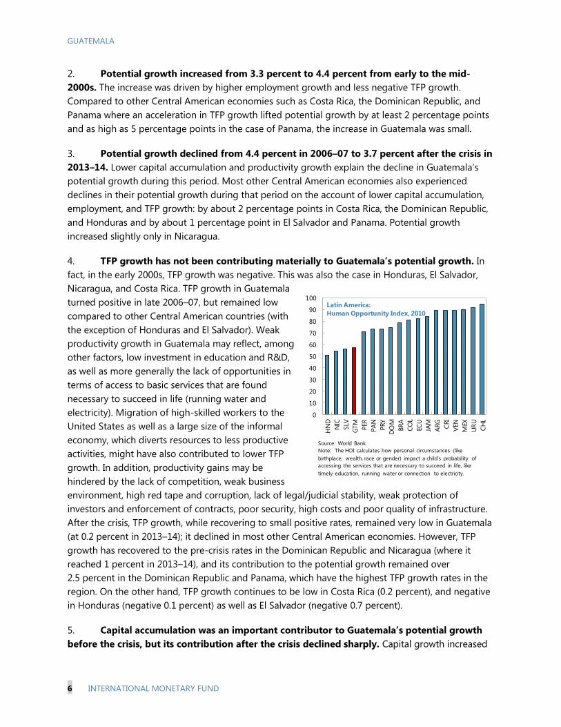
4. TFP growth has not been contributing materially to Guatemala’s potential growth. In
fact, in the early 2000s, TFP growth was negative. This was also the case in Honduras, El Salvador,
Nicaragua, and Costa Rica. TFP growth in Guatemala
turned positive in late 2006–07, but remained low
compared to other Central American countries (with
the exception of Honduras and El Salvador). Weak
productivity growth in Guatemala may reflect, among
other factors, low investment in education and R&D,
as well as more generally the lack of opportunities in
terms of access to basic services that are found
necessary to succeed in life (running water and
electricity). Migration of high-skilled workers to the
United States as well as a large size of the informal
economy, which diverts resources to less productive
activities, might have also contributed to lower TFP
growth. In addition, productivity gains may be
hindered by the lack of competition, weak business
environment, high red tape and corruption, lack of legal/judicial stability, weak protection of
investors and enforcement of contracts, poor security, high costs and poor quality of infrastructure.
After the crisis, TFP growth, while recovering to small positive rates, remained very low in Guatemala
(at 0.2 percent in 2013–14); it declined in most other Central American economies. However, TFP
growth has recovered to the pre-crisis rates in the Dominican Republic and Nicaragua (where it
reached 1 percent in 2013–14), and its contribution to the potential growth remained over
2.5 percent in the Dominican Republic and Panama, which have the highest TFP growth rates in the
region. On the other hand, TFP growth continues to be low in Costa Rica (0.2 percent), and negative
in Honduras (negative 0.1 percent) as well as El Salvador (negative 0.7 percent).
5. Capital accumulation was an important contributor to Guatemala’s potential growth
before the crisis, but its contribution after the crisis declined sharply. Capital growth increased
0
10
20
30
40
50
60
70
80
90
100
HN
D
NIC
SLV
GTM
PER
PA
N
PRY
DO
M
BRA
CO
L
ECU
JAM
ARG
CRI
VEN
MEX
UR
U
CH
L
Latin America:
Human Opportunity Index, 2010
Source: World Bank.
Note: The HOI calculates how personal circumstances (like
birthplace, wealth, race or gender) impact a child’s probability of
accessing the services that are necessary to succeed in life, like
timely education, running water or connection to electricity.

GUATEMALA
INTERNATIONAL MONETARY FUND 7
from 4.5 percent in the mid-2000s to 5.5 percent in 2007. A large decline in capital growth
accounted for most of the decline in potential growth in Guatemala after the crisis. Capital growth
dropped over 2.5 percentage points from 2006–07 to 2013–14, one of the largest declines in Central
America.
6. Employment growth, higher than elsewhere in the region, has been the main driver of
potential growth in Guatemala over the past decade. It increased from 3.3 percent to 3.5 percent
during the 2001–07, mainly attributable to higher working-age population growth. Fertility rates and
population growth in Guatemala are one of the highest in Central America and life expectancy has
been steadily increasing, which can explain in part the high growth in working-age population.
Potential employment growth continued increasing in Guatemala after the crisis. It increased by
about 0.3 percentage points (from 3.5 percent in 2007 to 3.8 percent in 2014), while other Central
American economies went through important declines in potential employment growth.
7. From a cyclical perspective, the
Guatemalan economy is assessed to be operating
at potential in 2015/16. The negative output gap in
Guatemala in 2009 (negative 1.2 percent of potential
output) has significantly shrunk and the slack in the
economy has been reduced since then. Both the
output gap and the unemployment gap (see
Appendix for details of the calculation) are now
closed. The closed unemployment gap reflects
improved labor conditions, where the unemployment
rate is at its equilibrium value having steadily fallen
since 2009.
8. Potential growth in Guatemala is likely to increase to 4 percent in the medium term.
The scenario analysis builds on the analysis of potential growth until 2014 and extends it 2015–2020,
-2%
0%
2%
4%
6%
8%
10%
12%
2001
-02
2006-0
7
2013
-14
2001-0
2
2006
-07
2013-1
4
2001
-02
2006-0
7
2013
-14
2001
-02
2006
-07
2013-1
4
2001-0
2
2006
-07
2013
-14
2001
-02
2006-0
7
2013
-14
2001-0
2
2006
-07
2013-1
4
2001-0
2
2006
-07
2013
-14
Capital
Labor
TFP
Potential output growth
Determinants of Potential Output Growth
(% and contributions to potential output growth, average for the period)
EMs PAN DOM CRI HNDGTM NICSLV
Source: IMF staff estimates.
-1.0%
-0.8%
-0.6%
-0.4%
-0.2%
0.0%
0.2%
0.4%
0.6%
0.8%
20
14
20
15
20
16
20
14
20
15
20
16
20
14
20
15
20
16
20
14
20
15
20
16
20
14
20
15
20
16
20
14
20
15
20
16
20
14
20
15
20
16
Output gap (% of potential output)
SLV GTM PAN DOM NIC HND CRI
Source: IMF staff estimates.

GUATEMALA
8 INTERNATIONAL MONETARY FUND
based on the projected demographic patterns, prospects for capital growth and improvements in
TFP growth. These scenarios are subject to significant uncertainty, as a number of country-specific
factors could influence potential growth, and the
evolution of TFP growth in the medium term. The
working-age population growth and labor force
participation growth are likely to continue at
similar rates. Investment-to-capital ratios have not
changed much since 2011 and are likely to remain
below pre-crisis rates, while improving only slightly
over the medium term given improvements in the
efficiency of public investment. This is because of
less favorable external financing conditions, and
weaknesses in the institutional, regulatory, and legal environment. TFP growth is expected to slightly
increase towards the end of the horizon driven by improvements in institutions providing legal and
judicial certainty, and a reduction in corruption.
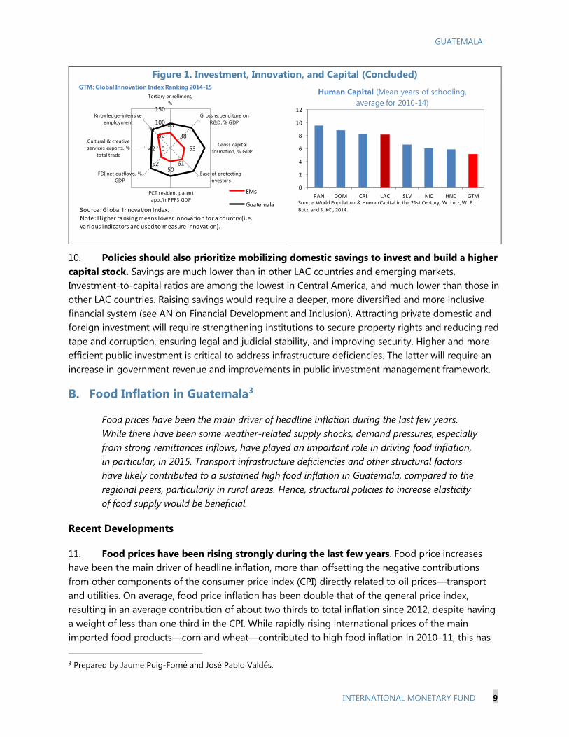
9. The main challenge in the longer term in Guatemala is to foster TFP growth. Relative to
the region and emerging markets, Guatemala performs poorly in various facets of innovation such
as spending on R&D, tertiary enrollment rates, number of patent applications, FDI inflows, ease of
protecting investors, knowledge-intensive employment, and creative services exports. Enhancing
R&D/technological diffusion will require strengthening institutions, human capital and research, and
achieving higher business and market sophistication, and competition in product and labor markets.
Adopting the Competition Law currently under consideration and sanctioning anti-competitive
behavior would support entry of new innovative firms and punish practices protecting incumbents.
Important improvements in the quality of schooling will also be needed to enhance human capital.
Figure 1. Investment, Innovation, and Capital
0
5
10
15
20
25
30
35
40
PAN HND DOM NIC CRI GTM SLV
Private
Public
FDI
LAC Private
LAC Public
LAC FDI
Investment
(Percent of GDP, 2014)
0
5
10
1. Fiscal Rules2. National &
Sectoral Planning
3. Central-Local
Coord ination
4. Management
of PP Ps
5. Company
Regulation
6. Multiyear
Budgeting
7. B udget
Comprehensive…
8. B udget Unity9. Project
Appraisal
10. Project
Selection
11. Protection of
Investment
12. Availability of
Funding
13.Transparency
of Execu tion
14.Project
Management
15. Monitoring
of Assets
GTM
LA5Public Investment Management in LAC
-1.0%
0.0%
1.0%
2.0%
3.0%
4.0%
5.0%
2001-07 2008-14 2015-20
K L Potential TFP Growth Potential Growth
GTM: Components of Potential Output Growth (%)
Source: IMF staff estimates.
GUATEMALA
INTERNATIONAL MONETARY FUND 9
Figure 1. Investment, Innovation, and Capital (Concluded)
10. Policies should also prioritize mobilizing domestic savings to invest and build a higher
capital stock. Savings are much lower than in other LAC countries and emerging markets.
Investment-to-capital ratios are among the lowest in Central America, and much lower than those in
other LAC countries. Raising savings would require a deeper, more diversified and more inclusive
financial system (see AN on Financial Development and Inclusion). Attracting private domestic and
foreign investment will require strengthening institutions to secure property rights and reducing red
tape and corruption, ensuring legal and judicial stability, and improving security. Higher and more
efficient public investment is critical to address infrastructure deficiencies. The latter will require an
increase in government revenue and improvements in public investment management framework.
B. Food Inflation in Guatemala3
Food prices have been the main driver of headline inflation during the last few years.
While there have been some weather-related supply shocks, demand pressures, especially
from strong remittances inflows, have played an important role in driving food inflation,
in particular, in 2015. Transport infrastructure deficiencies and other structural factors
have likely contributed to a sustained high food inflation in Guatemala, compared to the
regional peers, particularly in rural areas. Hence, structural policies to increase elasticity
of food supply would be beneficial.
Recent Developments
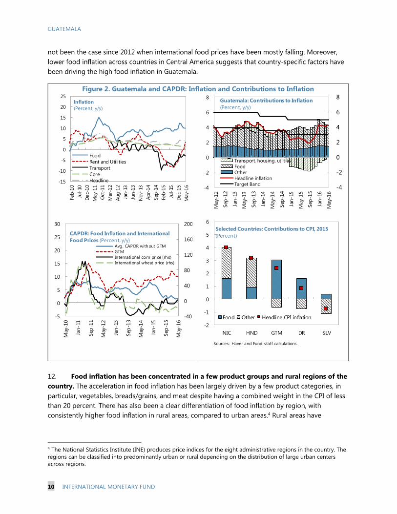
11. Food prices have been rising strongly during the last few years. Food price increases
have been the main driver of headline inflation, more than offsetting the negative contributions
from other components of the consumer price index (CPI) directly related to oil prices—transport
and utilities. On average, food price inflation has been double that of the general price index,
resulting in an average contribution of about two thirds to total inflation since 2012, despite having
a weight of less than one third in the CPI. While rapidly rising international prices of the main
imported food products—corn and wheat—contributed to high food inflation in 2010–11, this has
3 Prepared by Jaume Puig-Forné and José Pablo Valdés.
60
38
53
6150
52
42
71
0
50
100
150
Tertiary enrollment,
%
Gross expenditure on
R&D, % GDP
Gross capital
formation, % GDP
Ease of protect ing
investors
PCT resident patent
app./tr PPP$ GDP
FDI net outflows, %
GDP
Cultural & creative
services exports, %
total t rade
Knowledge-intensive
employment
EMs
Guatemala
GTM: Global Innovation Index Ranking 2014-15
Source: Global Innovation Index.Note: Higher ranking means lower innovation for a country (i .e.
various indicators are used to measure innovation).
0
2
4
6
8
10
12
PAN DOM CRI LAC SLV NIC HND GTM
Human Capital (Mean years of schooling,
average for 2010-14)
Source: World Population & Human Capital in the 21st Century, W. Lutz, W. P.
Butz, and S. KC., 2014.
GUATEMALA
10 INTERNATIONAL MONETARY FUND
not been the case since 2012 when international food prices have been mostly falling. Moreover,
lower food inflation across countries in Central America suggests that country-specific factors have
been driving the high food inflation in Guatemala.
Figure 2. Guatemala and CAPDR: Inflation and Contributions to Inflation
12. Food inflation has been concentrated in a few product groups and rural regions of the
country. The acceleration in food inflation has been largely driven by a few product categories, in
particular, vegetables, breads/grains, and meat despite having a combined weight in the CPI of less
than 20 percent. There has also been a clear differentiation of food inflation by region, with
consistently higher food inflation in rural areas, compared to urban areas.4 Rural areas have
4 The National Statistics Institute (INE) produces price indices for the eight administrative regions in the country. The
regions can be classified into predominantly urban or rural depending on the distribution of large urban centers
across regions.
-15
-10
-5
0
5
10
15
20
25
Feb-1
0
Jul-
10
Dec-
10
May
-11
Oct
-11
Mar
-12
Aug-1
2
Jan-1
3
Jun-1
3
Nov-
13
Apr-
14
Sep
-14
Feb-1
5
Jul-
15
Dec-
15
May
-16
Food
Rent and Utilities
Transport
Core
Headline
Inflation
(Percent, y/y)
-4
-2
0
2
4
6
8
-4
-2
0
2
4
6
8
May
-12
Sep
-12
Jan-1
3
May
-13
Sep
-13
Jan-1
4
May
-14
Sep
-14
Jan-1
5
May
-15
Sep
-15
Jan-1
6
May
-16
Transport, housing, utilties
Food
Other
Headline inflation
Target Band
Guatemala: Contributions to Inflation
(Percent, y/y)
-40
0
40
80
120
160
200
-5
0
5
10
15
20
25
30
May
-10
Jan-1
1
Sep
-11
May
-12
Jan-1
3
Sep
-13
May
-14
Jan-1
5
Sep
-15
May
-16
Avg. CAPDR without GTM
GTM
International corn price (rhs)
International wheat price (rhs)
CAPDR: Food Inflation and International
Food Prices (Percent, y/y)
-2
-1
0
1
2
3
4
5
6
NIC HND GTM DR SLV
Food Other Headline CPI inflation
Selected Countries: Contributions to CPI, 2015
(Percent)
Sources: Haver and Fund staff calculations.

GUATEMALA
INTERNATIONAL MONETARY FUND 11
contributed almost half of overall food inflation at the national level during the last few years,
despite representing about one fourth of the national CPI.
Figure 3. Food Prices
Drivers of Food Inflation
13. Demand pressures, especially from remittances flows, have played an important role
in driving food inflation. While there have been some weather related shocks temporarily pushing
up prices of some vegetable products—especially in late 20155—demand factors, including strong
remittances growth, appear to have been the main driver of high food inflation in the last few years,
judging from high correlations of food inflation with the output gap and remittances growth. Prices
of food products that have been experiencing
important increases—especially vegetables and
meat that tend to be added to the basic diet as
incomes of poor households increase—are
particularly highly correlated with remittances
inflows. The strong growth in remittances,
significantly above other countries in the region
in 2015, likely contributed to ease budget
constraints of poorer families with high levels of
malnutrition.
5 Weather related shocks explain the sharp increase in prices of tomatoes and onions in late 2015. The shocks also
affected neighboring countries, resulting also in increased external demand for these products.
0
1
2
3
4
5
6
7
2012 2013 2014 2015
Vegetables Bread and grains
Meat Other food
Headline CPI inflation
Guatemala: Contribution of Food Groups to
Headline CPI Inflation, 2012-15 (Percent)
-
5
10
15
20
25
Jan-1
2
Jul-
12
Jan-1
3
Jul-
13
Jan-1
4
Jul-
14
Jan-1
5
Jul-
15
Jan-1
6
Guatemala: Food Prices by Region
(Percent, annual growth)
Urban Rural
0.1
0.2
0.3
0.5
0.4
0.4
-1.5
-0.5
0.5
1.5
2.5
3.5
4.5
Mar-12 Sep-12 Mar-13 Sep-13 Mar-14 Sep-14 Mar-15 Sep-15 Mar-16
Guatemala: Contributions to Food Inflation
(In percent)
Beef
Tomato Onion
Eggs
Total
Food

GUATEMALA
12 INTERNATIONAL MONETARY FUND
Figure 4. Drivers of Food Inflation
14. The greater incidence of food inflation in rural areas also points to the importance of
remittances. While a similar share of remittances goes to rural and urban areas (with about half of
households living in each of those areas), remittances represent a greater share of total income in
rural areas that tend to be significantly poorer. Also, compared to urban areas, a much larger share
of remittances goes to the mid- and lower-end of the income distribution. Lower income
households spend a larger share of their income on food—almost 60 percent of total household
consumption in the lowest quintile, compared to about 35 percent in the highest quintile.
Figure 5. Remittances and Share of Food by Household Quintiles
1/ Based on distribution of per capita annual consumption.
15. Other structural factors may also be contributing to high food inflation, especially in
rural areas. Guatemala has the lowest level of urbanization in Central America. Low public
investment (Section a) resulting in transport infrastructure deficiencies that are particularly acute in
-0.5
0.0
0.5
1.0Food
Vegetables
MeatDairy
Bread/cereals
Remittances Brecha IMAE
Salaries Consumer credit
Correlations with Food Inflation (2012-15)
0
20
40
60
80
0
5
10
15
20
25
30
GTM DR HND NIC SLV
Remittances (yoy growth)
Share in CPI
Malnutrition - Height for age (rhs)
Growth of Remittances, Malnutrition, and
Share of Basic Food Prices in CPI
(Percent, 2015)
0
10
20
30
40
50
60
70
80
90
Urban Rural
1st Quintile 2nd Quintile
3rd Quintile 4th Quintile
Remittances by Household Quintiles 1/
(Percent of total in each region)
0
10
20
30
40
50
60
70
1st
Quintile
2nd
Quintile
3rd
Quintile
4th
Quintile
5th
Quintile
Share of Food in Total Consumption 1/
(Percent)
GUATEMALA
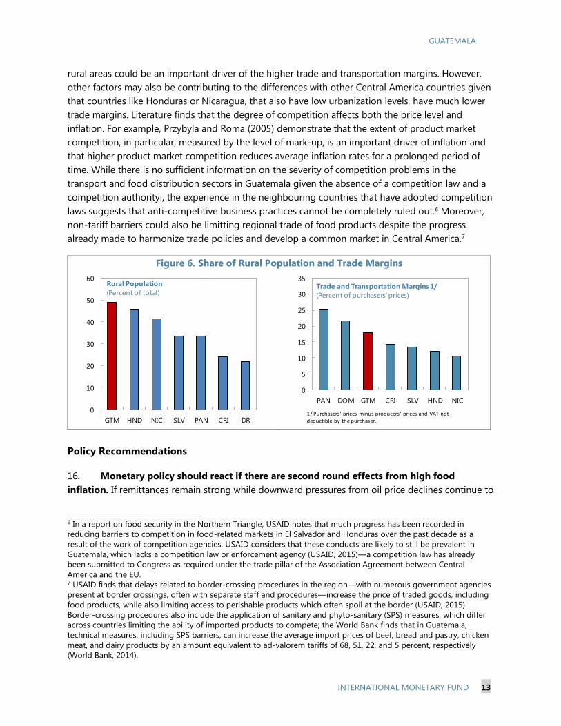
INTERNATIONAL MONETARY FUND 13
rural areas could be an important driver of the higher trade and transportation margins. However,
other factors may also be contributing to the differences with other Central America countries given
that countries like Honduras or Nicaragua, that also have low urbanization levels, have much lower
trade margins. Literature finds that the degree of competition affects both the price level and
inflation. For example, Przybyla and Roma (2005) demonstrate that the extent of product market
competition, in particular, measured by the level of mark-up, is an important driver of inflation and
that higher product market competition reduces average inflation rates for a prolonged period of
time. While there is no sufficient information on the severity of competition problems in the
transport and food distribution sectors in Guatemala given the absence of a competition law and a
competition authorityi, the experience in the neighbouring countries that have adopted competition
laws suggests that anti-competitive business practices cannot be completely ruled out.6 Moreover,
non-tariff barriers could also be limitting regional trade of food products despite the progress
already made to harmonize trade policies and develop a common market in Central America.7
Figure 6. Share of Rural Population and Trade Margins
Policy Recommendations
16. Monetary policy should react if there are second round effects from high food
inflation. If remittances remain strong while downward pressures from oil price declines continue to
6 In a report on food security in the Northern Triangle, USAID notes that much progress has been recorded in
reducing barriers to competition in food-related markets in El Salvador and Honduras over the past decade as a
result of the work of competition agencies. USAID considers that these conducts are likely to still be prevalent in
Guatemala, which lacks a competition law or enforcement agency (USAID, 2015)—a competition law has already
been submitted to Congress as required under the trade pillar of the Association Agreement between Central
America and the EU. 7 USAID finds that delays related to border-crossing procedures in the region—with numerous government agencies
present at border crossings, often with separate staff and procedures—increase the price of traded goods, including
food products, while also limiting access to perishable products which often spoil at the border (USAID, 2015).
Border-crossing procedures also include the application of sanitary and phyto-sanitary (SPS) measures, which differ
across countries limiting the ability of imported products to compete; the World Bank finds that in Guatemala,
technical measures, including SPS barriers, can increase the average import prices of beef, bread and pastry, chicken
meat, and dairy products by an amount equivalent to ad-valorem tariffs of 68, 51, 22, and 5 percent, respectively
(World Bank, 2014).
0
10
20
30
40
50
60
GTM HND NIC SLV PAN CRI DR
Rural Population
(Percent of total)
0
5
10
15
20
25
30
35
PAN DOM GTM CRI SLV HND NIC
Trade and Transportation Margins 1/
(Percent of purchasers' prices)
1/ Purchasers' prices minus producers' prices and VAT not deductible by the purchaser.
GUATEMALA
14 INTERNATIONAL MONETARY FUND
dissipate, sustained high food price inflation—particularly in rural areas where remittances play a
disproportionately greater role in final demand and where food supply is more inelastic—could
drive overall inflation above target. If this is seen as a temporary development, there is no need for
monetary policy to react, but if it has second round effects on inflation expectations or core
inflation, monetary tightening would be warranted (see AN on Monetary Policy Management).
17. Structural policies to increase supply of food, particularly in rural areas, could also
help.
Investments in transport infrastructure should be prioritized. This will facilitate access to national
food and other markets for those living in rural areas.
The new competition law should be adopted and a competition authority should be established
promptly. The new competition authority should prioritize analysis of food and transport
industries to determine whether issues within its mandate are contributing to the relatively
higher trade and transport margins in food prices compared to other countries in the region.
Improvements in customs procedures would not only be beneficial for competitiveness of
exporters, but could also remove one of the constraints on greater imports of perishable
products.
Additional advances in regional integration—beyond tariff reductions already implemented—to
reduce other non-tariff barriers, including SPS regulations would be helpful.8
Programs for rural development and poverty reduction should be comprehensive, supporting
both capacity to increase food consumption—through transfers or other means—and to ensure
adequate supply of food, including through programs to improve access to irrigation, financing,
and technical assistance in the agricultural sector.
Finally, measures to improve the business climate would also help provide a more enabling
environment for remittances to be directed to investment, rather than consumption as is
currently the case, especially in rural areas.
8 For example, mutual recognition of food product registration approval by national food and health authorities
would help reduce time and investment for introduction of national food products in new regional export markets.
(continued)

GUATEMALA
INTERNATIONAL MONETARY FUND 15
C. Female Labor Force Participation in Guatemala9
In contrast to male labor force participation (LFP), which is high in Guatemala by
regional standards, female labor force participation is lower than that in other Latin
American countries, though at par with that in other CAPDR countries. Using evidence
from household surveys and cross-country data, this note examines the determinants of
female labor force participation and the factors behind a relatively low female LFP rate in
Guatemala. Income, education and fertility levels, are important determinants of female
LFP. Increasing access to education, investment in infrastructure and information
technology as well as taking measures to support working mothers with children could
help raise female LFP in Guatemala.
Guatemala’s Labor Market
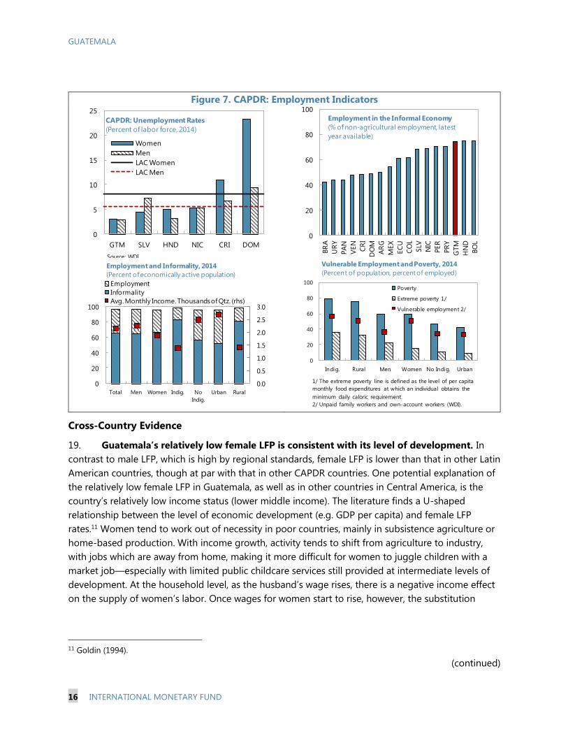
18. Guatemala’s labor market is characterized by low unemployment and high informality
and inequality, contributing to sub-par social outcomes. Unemployment is low and stable in
Guatemala, hovering around 3 percent during the last decade, with slightly higher rate for women
and slightly lower for men. High degree of informality and poor social protection schemes have
likely contributed to low unemployment rates in Guatemala. Inequality of labor conditions across
groups within the society is high, with the indigenous and rural populations having the highest rates
of informality and lowest average incomes, contributing to their higher poverty rates. Informality is
similar for women and men, although the average income is somewhat lower for women. The higher
share of vulnerable employment among women does not seem to be associated with worse social
outcomes, as they have similar poverty rates and significantly lower extreme poverty rates than
men.10
9 Prepared by Jaume Puig-Forne and Victoria Valente. 10 Vulnerable employment is defined in the World Bank Development Indicators as unpaid family workers and own-
account workers.
GUATEMALA
16 INTERNATIONAL MONETARY FUND
Figure 7. CAPDR: Employment Indicators
Cross-Country Evidence
19. Guatemala’s relatively low female LFP is consistent with its level of development. In
contrast to male LFP, which is high by regional standards, female LFP is lower than that in other Latin
American countries, though at par with that in other CAPDR countries. One potential explanation of
the relatively low female LFP in Guatemala, as well as in other countries in Central America, is the
country’s relatively low income status (lower middle income). The literature finds a U-shaped
relationship between the level of economic development (e.g. GDP per capita) and female LFP
rates.11 Women tend to work out of necessity in poor countries, mainly in subsistence agriculture or
home-based production. With income growth, activity tends to shift from agriculture to industry,
with jobs which are away from home, making it more difficult for women to juggle children with a
market job—especially with limited public childcare services still provided at intermediate levels of
development. At the household level, as the husband’s wage rises, there is a negative income effect
on the supply of women’s labor. Once wages for women start to rise, however, the substitution
11 Goldin (1994).
(continued)
0
5
10
15
20
25
GTM SLV HND NIC CRI DOM
Women
Men
LAC Women
LAC Men
Source: WDI
CAPDR: Unemployment Rates
(Percent of labor force, 2014)
0
20
40
60
80
100
BR
A
UR
Y
PA
N
VEN
CR
I
DO
M
AR
G
MEX
EC
U
CO
L
SLV
NIC
PER
PR
Y
GTM
HN
D
BO
L
Employment in the Informal Economy
(% of non-agricultural employment, latest
year available)
0.0
0.5
1.0
1.5
2.0
2.5
3.0
0
20
40
60
80
100
Total Men Women Indig. No
Indig.
Urban Rural
Employment
Informality
Avg. Monthly Income. Thousands of Qtz. (rhs)
Employment and Informality, 2014
(Percent ofeconomically active population)
0
20
40
60
80
100
Indig. Rural Men Women No Indig. Urban
Poverty
Extreme poverty 1/
Vulnerable employment 2/
Vulnerable Employment and Poverty, 2014
(Percent of population, percent of employed)
1/ The extreme poverty line is defined as the level of per capita
monthly food expenditures at which an individual obtains the
minimum daily caloric requirement.
2/ Unpaid family workers and own-account workers (WDI).
GUATEMALA
INTERNATIONAL MONETARY FUND 17
effect increases incentives for women to increase their labor supply, until this effect dominates the
negative income effect.12
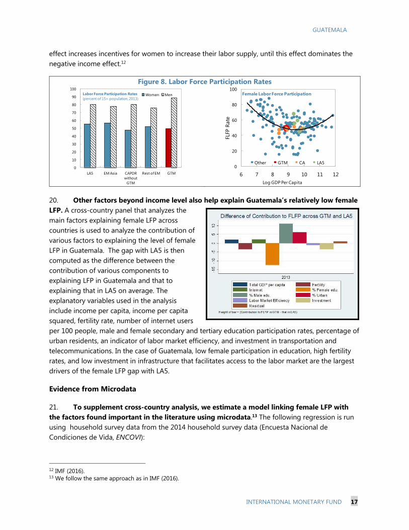
Figure 8. Labor Force Participation Rates
20. Other factors beyond income level also help explain Guatemala’s relatively low female
LFP. A cross-country panel that analyzes the
main factors explaining female LFP across
countries is used to analyze the contribution of
various factors to explaining the level of female
LFP in Guatemala. The gap with LA5 is then
computed as the difference between the
contribution of various components to
explaining LFP in Guatemala and that to
explaining that in LA5 on average. The
explanatory variables used in the analysis
include income per capita, income per capita
squared, fertility rate, number of internet users
per 100 people, male and female secondary and tertiary education participation rates, percentage of
urban residents, an indicator of labor market efficiency, and investment in transportation and
telecommunications. In the case of Guatemala, low female participation in education, high fertility
rates, and low investment in infrastructure that facilitates access to the labor market are the largest
drivers of the female LFP gap with LA5.
Evidence from Microdata
21. To supplement cross-country analysis, we estimate a model linking female LFP with
the factors found important in the literature using microdata.13 The following regression is run
using household survey data from the 2014 household survey data (Encuesta Nacional de
Condiciones de Vida, ENCOVI):
12 IMF (2016). 13 We follow the same approach as in IMF (2016).
0
10
20
30
40
50
60
70
80
90
100
LA5 EM Asia CAPDR
without
GTM
Rest of EM GTM
Women MenLabor Force Participation Rates
(percent of 15+ population, 2013)
0
20
40
60
80
100
6 7 8 9 10 11 12
FLFP
Rate
Log GDP Per Capita
Other GTM CA LA5
Female Labor Force Participation
GUATEMALA
18 INTERNATIONAL MONETARY FUND
𝐹𝐿𝐹𝑃𝑖𝑟𝑡 = 𝛼 + 𝛽1𝑝𝑟𝑖𝑚_𝑠𝑒𝑐𝑜𝑛𝑑_𝑒𝑑𝑢𝑖 + 𝛽2𝑠𝑒𝑐𝑜𝑛𝑑_𝑡𝑒𝑟𝑡𝑖𝑎𝑟𝑦_𝑒𝑑𝑢𝑖 + 𝛽3 𝑚𝑜𝑟𝑒_𝑡ℎ𝑎𝑛_𝑡𝑒𝑟𝑡𝑖𝑎𝑟𝑦_𝑒𝑑𝑢𝑖
+ 𝛽4𝑢𝑟𝑏𝑎𝑛𝑖 + 𝛽5𝑚𝑎𝑟𝑟𝑖𝑒𝑑𝑖 + 𝛽6𝑎𝑔𝑒𝑖 + 𝛽7(𝑎𝑔𝑒)𝑖2 + 𝛽8 𝑐𝑒𝑙𝑙𝑝ℎ𝑜𝑛𝑒𝑖 + 𝛽9𝑐𝑜𝑚𝑝𝑢𝑡𝑒𝑟𝑖
+ 𝛽10𝑘𝑖𝑑_0𝑡𝑜6𝑖 + 𝛽11𝑘𝑖𝑑_6𝑡𝑜12𝑖 + 𝛽12𝑜𝑙𝑑_𝑚𝑜𝑟𝑒𝑡ℎ𝑎𝑛_70𝑖 + 𝛽13log (ℎ𝑒𝑎𝑑𝑖𝑛𝑐𝑜𝑚𝑒)𝑖 + 𝛾𝑟
+ 휀𝑖𝑟
where 𝑝𝑟𝑖𝑚_𝑠𝑒𝑐𝑜𝑛𝑑_𝑒𝑑𝑢𝑖, 𝑠𝑒𝑐𝑜𝑛𝑑_𝑡𝑒𝑟𝑡𝑖𝑎𝑟𝑦_𝑒𝑑𝑢𝑖, and 𝑚𝑜𝑟𝑒_𝑡ℎ𝑎𝑛_𝑡𝑒𝑟𝑡𝑖𝑎𝑟𝑦_𝑒𝑑𝑢𝑖 are dummy variables
for the woman i's final educational attainment level, and 𝑢𝑟𝑏𝑎𝑛𝑖, 𝑚𝑎𝑟𝑟𝑖𝑒𝑑𝑖, 𝑐𝑒𝑙𝑙𝑝ℎ𝑜𝑛𝑒𝑖, and
𝑐𝑜𝑚𝑝𝑢𝑡𝑒𝑟𝑖 are dummy variables for the location of the household in urban area, household being a
married couple, and household having a cell-phone. 𝑘𝑖𝑑_0𝑡𝑜6, 𝑘𝑖𝑑_6𝑡𝑜12𝑖, and 𝑜𝑙𝑑_𝑚𝑜𝑟𝑒𝑡ℎ𝑎𝑛_70𝑖 are
equal to one if a household has a member in these categories, respectively. log (ℎ𝑒𝑎𝑑𝑖𝑛𝑐𝑜𝑚𝑒)𝑖 is the
log of income of a household head? Regional fixed effects are also included.
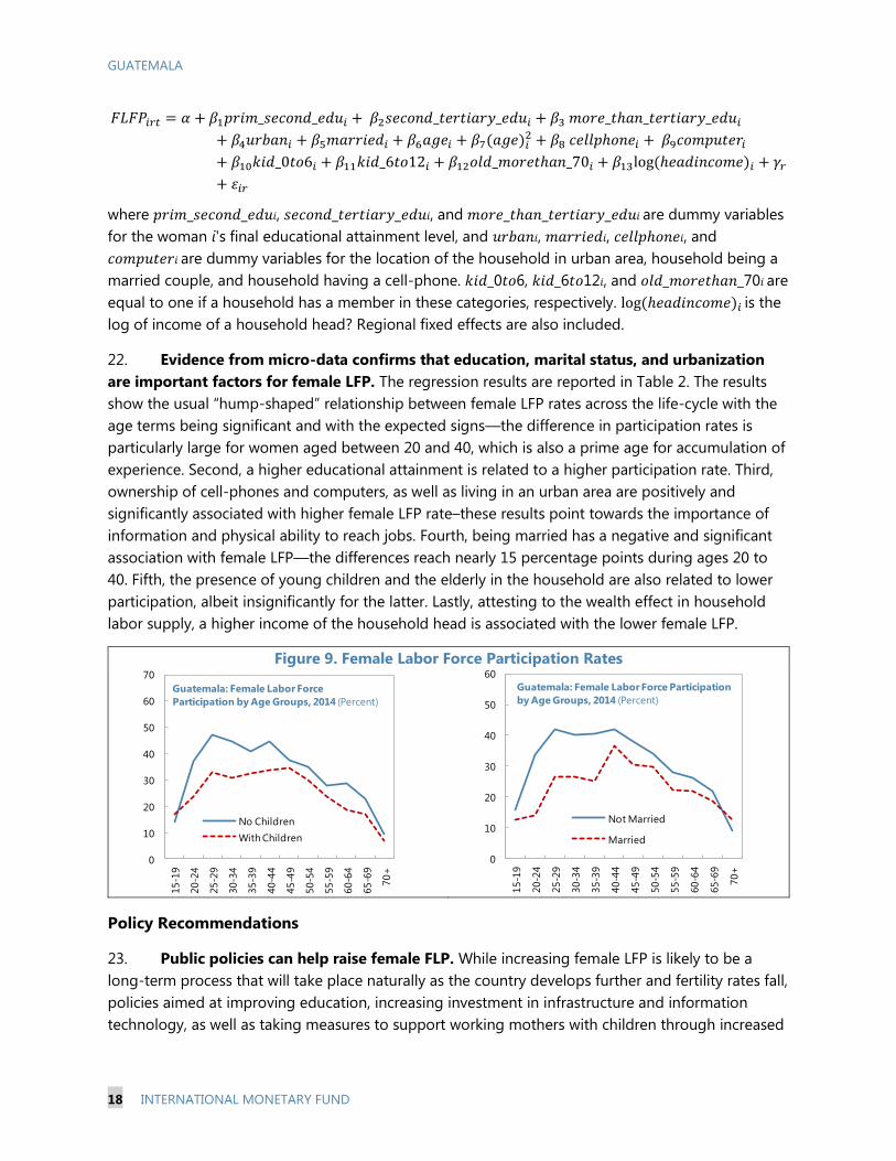
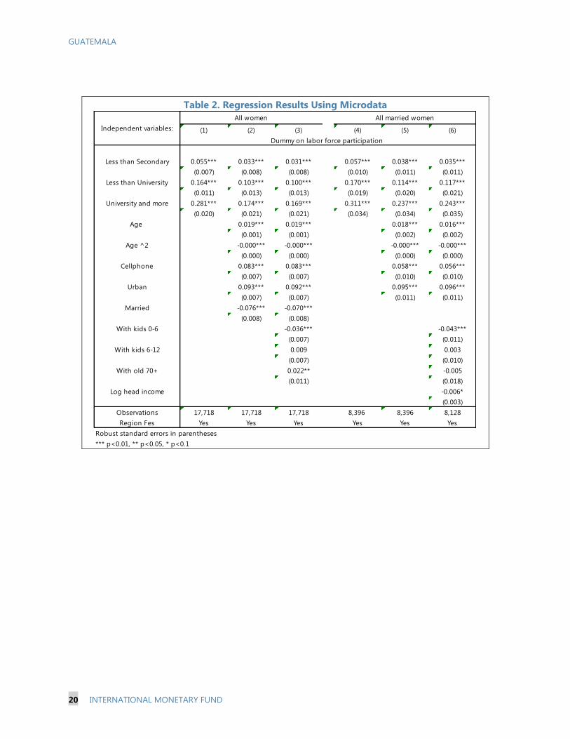
22. Evidence from micro-data confirms that education, marital status, and urbanization
are important factors for female LFP. The regression results are reported in Table 2. The results
show the usual “hump-shaped” relationship between female LFP rates across the life-cycle with the
age terms being significant and with the expected signs—the difference in participation rates is
particularly large for women aged between 20 and 40, which is also a prime age for accumulation of
experience. Second, a higher educational attainment is related to a higher participation rate. Third,
ownership of cell-phones and computers, as well as living in an urban area are positively and
significantly associated with higher female LFP rate–these results point towards the importance of
information and physical ability to reach jobs. Fourth, being married has a negative and significant
association with female LFP—the differences reach nearly 15 percentage points during ages 20 to
40. Fifth, the presence of young children and the elderly in the household are also related to lower
participation, albeit insignificantly for the latter. Lastly, attesting to the wealth effect in household
labor supply, a higher income of the household head is associated with the lower female LFP.
Figure 9. Female Labor Force Participation Rates
Policy Recommendations
23. Public policies can help raise female FLP. While increasing female LFP is likely to be a
long-term process that will take place naturally as the country develops further and fertility rates fall,
policies aimed at improving education, increasing investment in infrastructure and information
technology, as well as taking measures to support working mothers with children through increased
0
10
20
30
40
50
60
70
15-1
9
20-2
4
25-2
9
30-3
4
35-3
9
40-4
4
45-4
9
50-5
4
55-5
9
60-6
4
65-6
9
70+
No Children
With Children
Guatemala: Female Labor Force
Participation by Age Groups, 2014 (Percent)
0
10
20
30
40
50
60
15-1
9
20-2
4
25-2
9
30-3
4
35-3
9
40-4
4
45-4
9
50-5
4
55-5
9
60-6
4
65-6
9
70+
Not Married
Married
Guatemala: Female Labor Force Participation
by Age Groups, 2014 (Percent)
GUATEMALA
INTERNATIONAL MONETARY FUND 19
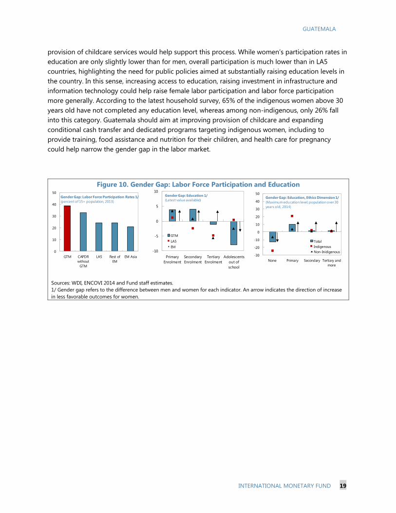
provision of childcare services would help support this process. While women’s participation rates in
education are only slightly lower than for men, overall participation is much lower than in LA5
countries, highlighting the need for public policies aimed at substantially raising education levels in
the country. In this sense, increasing access to education, raising investment in infrastructure and
information technology could help raise female labor participation and labor force participation
more generally. According to the latest household survey, 65% of the indigenous women above 30
years old have not completed any education level, whereas among non-indigenous, only 26% fall
into this category. Guatemala should aim at improving provision of childcare and expanding
conditional cash transfer and dedicated programs targeting indigenous women, including to
provide training, food assistance and nutrition for their children, and health care for pregnancy
could help narrow the gender gap in the labor market.
Figure 10. Gender Gap: Labor Force Participation and Education
Sources: WDI, ENCOVI 2014 and Fund staff estimates.
1/ Gender gap refers to the difference between men and women for each indicator. An arrow indicates the direction of increase
in less favorable outcomes for women.
0
10
20
30
40
50
GTM CAPDR
without
GTM
LA5 Rest of
EM
EM Asia
Gender Gap: Labor Force Participation Rates 1/
(percent of 15+ population, 2013)
-10
-5
0
5
10
Primary
Enrolment
Secondary
Enrolment
Tertiary
Enrolment
Adolescents
out of
school
GTM
LA5
EM
Gender Gap: Education 1/
(Latest value available)
-30
-20
-10
0
10
20
30
40
50
None Primary Secondary Tertiary and
more
Total
Indigenous
Non-Inidigenous
Gender Gap: Education, Ethics Dimension 1/
(Maximum education level, population over 30
years old, 2014)
GUATEMALA
20 INTERNATIONAL MONETARY FUND
Table 2. Regression Results Using Microdata
(1) (2) (3) (4) (5) (6)
Less than Secondary 0.055*** 0.033*** 0.031*** 0.057*** 0.038*** 0.035***
(0.007) (0.008) (0.008) (0.010) (0.011) (0.011)
Less than University 0.164*** 0.103*** 0.100*** 0.170*** 0.114*** 0.117***
(0.011) (0.013) (0.013) (0.019) (0.020) (0.021)
University and more 0.281*** 0.174*** 0.169*** 0.311*** 0.237*** 0.243***
(0.020) (0.021) (0.021) (0.034) (0.034) (0.035)
Age 0.019*** 0.019*** 0.018*** 0.016***
(0.001) (0.001) (0.002) (0.002)
Age ^2 -0.000*** -0.000*** -0.000*** -0.000***
(0.000) (0.000) (0.000) (0.000)
Cellphone 0.083*** 0.083*** 0.058*** 0.056***
(0.007) (0.007) (0.010) (0.010)
Urban 0.093*** 0.092*** 0.095*** 0.096***
(0.007) (0.007) (0.011) (0.011)
Married -0.076*** -0.070***
(0.008) (0.008)
With kids 0-6 -0.036*** -0.043***
(0.007) (0.011)
With kids 6-12 0.009 0.003
(0.007) (0.010)
With old 70+ 0.022** -0.005
(0.011) (0.018)
Log head income -0.006*
(0.003)
Observations 17,718 17,718 17,718 8,396 8,396 8,128
Region Fes Yes Yes Yes Yes Yes Yes
Robust standard errors in parentheses
*** p<0.01, ** p<0.05, * p<0.1
All women All married women
Dummy on labor force participation
Independent variables:
GUATEMALA
INTERNATIONAL MONETARY FUND 21
References
Attanasio, Orazio, Hamish Low, and Virginia Sanchez-Marcos. 2008. "Explaining Changes in Female
Labor Supply in a Life-Cycle Model." American Economic Review, 98(4): 1517-52.
Bloom, David E, David Canning, Gunther Fink, and Jocelyn E. Finlay. (2007) “Fertility, Female Labor
Force Participation, and the Demographic Dividend.” NBER Working Paper #13583.
Goldin, Claudia. (1994) “The U-shaped Female Labor Force Function in Economic Development and
Economic History.” NBER Working Paper #2707.
International Monetary Fund. (2016) “Costa Rica Selected Issues and Analytical Notes,” Analytical
Note IV, IMF Country Report No. 16/132.
Kelleher, Sinéad and Reyes, José-Daniel. (2014) “Technical measures to trade in Central America:
incidence, price effects, and consumer welfare” World Bank Policy Research Working Paper
6857.
Przybyla and Roma, (2005) “Does Product Market Competition Reduce Inflation? Evidence from EU
Countries and Sectors,” European Central Bank working paper No. 453.
USAID. (2015) “A Report on Barriers to Competition in Food-Related Markets in El Salvador,
Guatemala, and Honduras.”
GUATEMALA
22 INTERNATIONAL MONETARY FUND
Appendix. Multivariate Filter Methodology
The multivariate filter approach specified in this selected issues paper requires data on three
observable variables: real GDP growth, CPI inflation, and the unemployment rate. Annual data is
used for these variables for the 7 countries considered. In this section, we present the equations
which relate these three observable variables to the latent variables in the model. Parameter values
and the variances of shock terms for these equations are estimated using Bayesian estimation
techniques.
In the model, the output gap is defined as the deviation of real GDP, in log terms (𝑌), from its
potential level (𝑌):
𝑦 = 𝑌 − 𝑌
The stochastic process for output (real GDP) is comprised of three equations, and subject to three
types of shocks:
𝑌𝑡 = 𝑌𝑡−1 + 𝐺𝑡 + 휀𝑡𝑌
𝐺𝑡 = 𝜃𝐺𝑆𝑆 + (1 − 𝜃)𝐺𝑡−1 + 휀𝑡𝐺
𝑦𝑡 = 𝜙𝑦𝑡−1 + 휀𝑡𝑦
The level of potential output (𝑌𝑡) evolves according to potential growth (𝐺𝑡) and a level-shock term
(휀𝑡𝑌). Potential growth is also subject to shocks (휀𝑡
𝐺), with their impact fading gradually according to
the parameter 𝜃 (with lower values entailing a slower adjustment back to the steady-state growth
rate following a shock). Finally, the output-gap is also subject to shocks (휀𝑡𝑦
), which are effectively
demand shocks.
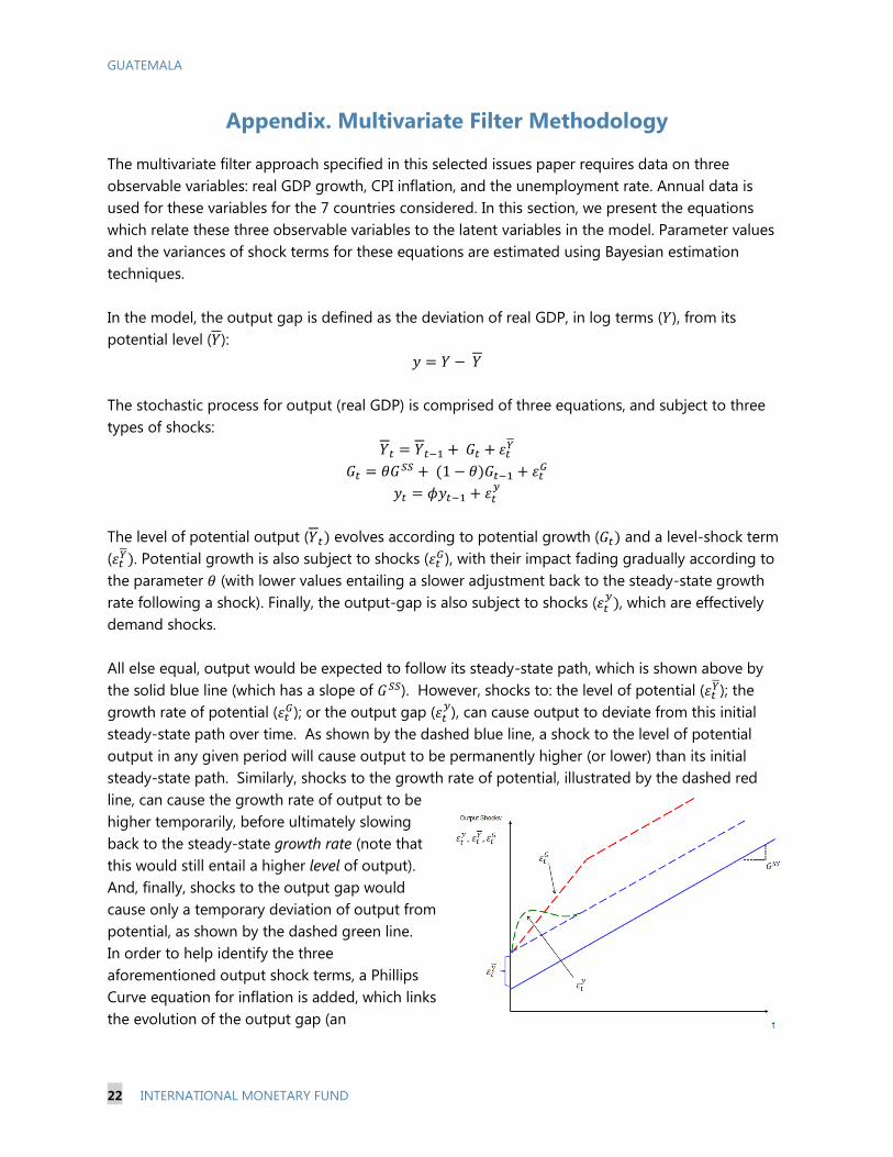
All else equal, output would be expected to follow its steady-state path, which is shown above by
the solid blue line (which has a slope of 𝐺𝑆𝑆). However, shocks to: the level of potential (휀𝑡𝑌); the
growth rate of potential (휀𝑡𝐺); or the output gap (휀𝑡
𝑦), can cause output to deviate from this initial
steady-state path over time. As shown by the dashed blue line, a shock to the level of potential
output in any given period will cause output to be permanently higher (or lower) than its initial
steady-state path. Similarly, shocks to the growth rate of potential, illustrated by the dashed red
line, can cause the growth rate of output to be
higher temporarily, before ultimately slowing
back to the steady-state growth rate (note that
this would still entail a higher level of output).
And, finally, shocks to the output gap would
cause only a temporary deviation of output from
potential, as shown by the dashed green line.
In order to help identify the three
aforementioned output shock terms, a Phillips
Curve equation for inflation is added, which links
the evolution of the output gap (an

GUATEMALA
INTERNATIONAL MONETARY FUND 23
unobservable variable) to observable data on inflation according to the process:
𝜋𝑡 = 𝜆𝜋𝑡+1 + (1 − 𝜆)𝜋𝑡−1 + 𝛽𝑦𝑡 + 휀𝑡𝜋
Finally, equations describing the evolution of unemployment are included to provide further
identifying information for the estimation of the output gap:
𝑈𝑡 = (𝜏4 𝑈𝑠𝑠
+ (1 − 𝜏4)𝑈𝑡−1) + 𝑔𝑈𝑡
+ 휀𝑡𝑈
𝑔𝑈𝑡 = (1 − 𝜏3)𝑔𝑈𝑡−1 + 휀𝑡𝑔𝑈
𝑢𝑡 = 𝜏2𝑢𝑡−1 + 𝜏1𝑦𝑡 + 휀𝑡𝑢
𝑢𝑡 = 𝑈𝑡 − 𝑈𝑡
Here, 𝑈𝑡 is the equilibrium value of the unemployment rate (the NAIRU), which is time varying, and
subject to shocks (휀𝑡𝑈) and also variation in the trend (𝑔𝑈𝑡), which is itself also subject to shocks
(휀𝑡𝑔𝑈
)—this specification allows for persistent deviations of the NAIRU from its steady-state value.
Most importantly, we specify an Okun’s law relationship wherein the unemployment gap between
actual unemployment (𝑈𝑡) and its equilibrium process (given by 𝑢𝑡) is a function of the amount of
slack in the economy (𝑦𝑡).
Equations 1–9 comprise the core of the model for potential output. In addition, data on growth and
inflation expectations are added, in part to help identify shocks, but mostly to improve the accuracy
of estimates at the end of the sample period:
𝜋𝑡+𝑗𝐶 = 𝜋𝑡+𝑗 + 휀𝑡+𝑗
𝜋𝐶 , j = 0,1
𝐺𝑅𝑂𝑊𝑇𝐻𝑡+𝑗𝐶 = 𝐺𝑅𝑂𝑊𝑇𝐻𝑡+𝑗 + 휀𝑡+𝑗
𝐺𝑅𝑂𝑊𝑇𝐻𝐶 , j = 0,…,5
For real GDP growth (𝐺𝑅𝑂𝑊𝑇𝐻) the model is augmented with forecasts from the WEO for the five
years following the end of the sample period. For inflation, expectations data are added for one
year following the end of the sample period. These equations relate the model-consistent forward
expectation for growth and inflation (𝜋𝑡+𝑗 and 𝐺𝑅𝑂𝑊𝑇𝐻𝑡+𝑗) to observable data on how WEO
forecasters expect these variables to evolve over various horizons (one to five years ahead) at any
given time (𝐺𝑅𝑂𝑊𝑇𝐻𝑡+𝑗𝐶 ). The ‘strength’ of the relationship between the data on the WEO forecasts
and the model’s forward expectation is determined by the standard deviation of the error terms
(휀𝑡+𝑗 𝜋𝐶
and 휀𝑡+𝑗 𝐺𝑅𝑂𝑊𝑇𝐻𝐶
). In practice, the estimated variance of these terms allows WEO data to
influence, but not completely override, the model’s expectations, particularly at the end of the
sample period. In a way, the incorporation of WEO forecasts can be thought as a heuristic approach
to blend forecasts from different sources and methods.
The methodology requires taking a stance on prior beliefs regarding a number of variables. A key
assumption fed into the model’s estimation is that supply shocks are the primary source of real GDP
fluctuations in Central America. The prior belief that supply is more volatile than demand leads the
model to assign much of the observed volatility of real GDP to potential GDP fluctuations. In

GUATEMALA
24 INTERNATIONAL MONETARY FUND
addition to the prior distributions of parameters, initial values for the steady-state (long-run)
unemployment rate and potential GDP growth rates are provided.
After obtaining estimates of potential output and NAIRU from the multivariate Kalman filter,
potential TFP is calculated as a residual in the Cobb-Douglas function:
1
t t t tA Y K L
where Yt is potential output, Kt and Lt are capital and labor inputs, while At is the contribution of
technology or TFP. Output elasticities (α is the capital share in the production function and is set at
0.35) sum up to one. Data on the working age population and the labor force participation rate is
obtained from the UN Economic Commission for Latin American and the Caribbean (CEPAL).
Potential employment is constructed as a product of working age population, the labor force
participation rate, and the employment rate (1-NAIRU).
The capital stock series is constructed using a perpetual inventory method where the level of initial
capital stock for a given year, 1990 in our case, is calculated assuming a constant level of
depreciation rate of 5 percent per annum and a constant investment share of GDP.
GUATEMALA
INTERNATIONAL MONETARY FUND 25
FISCAL POLICY: SUSTAINABILITY AND SOCIAL
OBJECTIVES
A. Fiscal Sustainability Assessment1
This section presents an assessment of Guatemala’s medium and long term debt sustainability.
The results suggest that under the current policies, central government debt is sustainable at
24 percent of GDP and even a short-term relaxation of the fiscal deficit by ½ percent of GDP
would only slightly increase the debt-to-GDP ratio in the longer term. Other alternative
scenarios based on a permanent relaxation by ½ percent of GDP, historical averages and a
large contingent liability shock also indicate debt stabilization in the longer term at levels
between 25 and 30 percent of GDP, respectively. The debt path is quite resilient to macro
shocks. While not an immediate concern, rising demographic pressures, if left unaddressed,
would pose challenges for the budget in the medium and long term.
Introduction
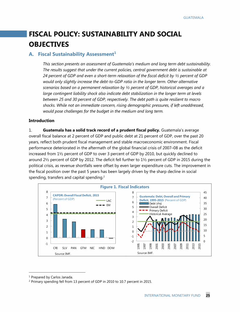
1. Guatemala has a solid track record of a prudent fiscal policy. Guatemala’s average
overall fiscal balance at 2 percent of GDP and public debt at 21 percent of GDP, over the past 20
years, reflect both prudent fiscal management and stable macroeconomic environment. Fiscal
performance deteriorated in the aftermath of the global financial crisis of 2007–08 as the deficit
increased from 1½ percent of GDP to over 3 percent of GDP by 2010, but quickly declined to
around 2½ percent of GDP by 2012. The deficit fell further to 1½ percent of GDP in 2015 during the
political crisis, as revenue shortfalls were offset by even larger expenditure cuts. The improvement in
the fiscal position over the past 5 years has been largely driven by the sharp decline in social
spending, transfers and capital spending.2
Figure 1. Fiscal Indicators
1 Prepared by Carlos Janada. 2 Primary spending fell from 13 percent of GDP in 2010 to 10.7 percent in 2015.
-1
0
1
2
3
4
5
6
7
8
CRI SLV PAN GTM NIC HND DOM
LAC
EM
CAPDR: Overall Fiscal Deficit, 2015
(Percent of GDP)
Source: IMF.
0
5
10
15
20
25
30
35
40
45
-2
-1
0
1
2
3
4
5
6
7
8
1995
1997
1999
2001
2003
2005
2007
2009
2011
2013
2015
Debt (rhs)
Overall Deficit
Primary Deficit
Historical Average
Guatemala: Debt, Overall and Primary
Deficit, 1995-2015 (Percent of GDP)
Source: IMF.

GUATEMALA
26 INTERNATIONAL MONETARY FUND
2. Guatemala’s debt is low as a share of GDP though it is moderately high in relation to
fiscal revenues. Public debt currently stands at 24½ percent of GDP. It has been virtually
unchanged over the last four years. This level compares favorably to other countries in the region
and to emerging market peers. Moreover, it is well below an indicative benchmark of 60 percent of
GDP for countries with market access.3 However, Guatemala’s position looks less favorable when
debt is compared to revenues since revenues are low by international standards.4
Figure 2. General Government Debt Indicators*
*In the case of Guatemala, it refers to Central Government.
3. Additional efforts to raise tax collections will be needed to ensure adequate provision
of basic public goods. Guatemala’s low revenue capacity constrains the level of government
spending, currently at 12 percent of GDP. However, literature finds that the optimal size of the
government, in particular, with respect to human development, is at least 15 percent of GDP.5
Hence, it would be desirable raising fiscal revenues to 15 percent of GDP in the medium term to
accommodate higher social and infrastructure spending as well as support efforts to durably reduce
crime and corruption. Improving tax performance, however, will require strong and sustained
political commitment at the highest levels. The 2012 tax reform provided additional tools for the
government to enforce tax controls and supervision, as well as eliminate VAT exemptions and
reduce rates of the corporate income tax while broadening its base. The additional revenue from the
2012 tax reform was envisaged at 1–1½ percent of GDP over the course of several years. However,
the reform ended up plagued by multiple legal challenges and administrative problems. Most
importantly, the customs agency faced significant administrative delays in implementing the reform,
3 See Annex II of the IMF “Staff Guidance Note for Public Debt Sustainability Analysis in Market Access Countries,”
2013 at https://www.imf.org/external/np/pp/eng/2013/050913.pdf. 4 Guatemala has one of the lowest revenue-to-GDP ratios in the world (see, for example. “Tax Capacity and Growth: Is
There a Tipping Point,” by Vitor Gaspar, Laura Jaramillo and Philippe Wingender; FAD Seminar Series, December 9,
2015. 5Peden, E. (1991), Karras, G. (1997), Davies (2009), Gunalp and Dincer (2005), On the upper side, estimates vary but
mainly fall below 30 percent of GDP.
0
20
40
60
80
100
SLV HND CRI PAN DOM NIC GTM
EM Average
Indicative Benchmark 3/
General Government Gross Debt
(Percent of GDP, 2015)
Source: IMF WEO Database.
0
50
100
150
200
250
300
350
400
NIC HND PAN DOM GTM CRI SLV
EM Average
General Government Gross Debt to Fiscal
Revenues (Percent, 2015)
Source: IMF WEO Database.

GUATEMALA
INTERNATIONAL MONETARY FUND 27
which were exacerbated by high staff turn-over. As a result, the revenue yield of the reform turned
out to be much lower than envisaged with virtually unchanged tax-to-GDP ratio after the reform.
Assessing Debt Dynamics and Fiscal Sustainability
4. The sustainability of public finances was analyzed under 5 alternative scenarios. The
first scenario (the baseline) assumes a relatively constant primary deficit of 0.1 percent of GDP (a
corresponding overall fiscal deficit of 1.6 percent of GDP). The second scenario assumes a temporary
relaxation (for 5 years) of the overall deficit to 2 percent of GDP—a historical average. The third
scenario assumes a primary balance consistent with a permanent relaxation of the overall fiscal
deficit to 2 percent of GDP. The fourth scenario assumes that real GDP growth rate, real interest rate
and the primary balance remain at their historical averages over the past ten years.6 The fifth
scenario assumes that a contingent liability shock of 10 percent of the size of commercial bank
assets must be accommodated by the budget.7
5. Fiscal position is sustainable in the long-run under all five scenarios but the debt ratio
is higher under the permanent relaxation, and contingent liability shock scenarios. In the
baseline scenario the debt-to-GDP ratio stabilizes at the current level of 24 percent of GDP in the
medium and long term; the debt-to-revenue ratio remains at around 210 percent. In the scenario of
temporary relaxation, the debt-to-GDP ratio rises slightly in the short term and stabilizes at
26 percent of GDP in the long term while debt-to-revenue ratio increases to 230 percent. In the
permanent relaxation scenario, the debt ratio continues rising over a long horizon but stabilizes at
28½ percent of GDP with the debt-to-revenue ratio reaching 250 percent. In the historical average
scenario debt to GDP ratio rises only to 24¾ percent of GDP and debt-to-revenue increases to 220
percent. Finally, in the contingent liability shock scenario the debt reaches a 30 percent of GDP level
faster than in the permanent relaxation scenario but remains stable thereafter, with the debt to
revenue slightly exceeding 260 percent. Under all five scenarios the debt-to-GDP does not exceed
an indicative benchmark for countries with market access at 60 percent.
6 The years of 2009 and 2010, when the effects of the global financial crisis affected Guatemala most deeply, were
excluded. The historical sample was extended by two earlier years to compensate (i.e., the historical average is still
based on a 10-year sample). 7 Commercial bank assets were roughly half of GDP at the end of 2015. Therefore, the contingent liability shock is
equivalent to 5 percent of GDP. As a reference, the Troubled Asset Relief Program (TARP) in the U.S. was equivalent
to about 5 percent of US GDP when it was announced during the financial crisis of 2008.

GUATEMALA
28 INTERNATIONAL MONETARY FUND
Figure 3. Long-Term Sustainability
1/ This path is the baseline through 2021, with a small primary deficit, which stabilizes the debt
ratio thereafter.
2/ Permanent relaxation begins in 2017. It has a primary deficit compatible with an overall deficit of
2 percent of GDP for the entire period.
3/ Temporary relaxation scenario runs a 2 percent of GDP overall deficit between 2017 and 2021,
the deficit declines thereafter.
-5
-4
-3
-2
-1
0
1
-0.6
-0.5
-0.4
-0.3
-0.2
-0.1
0.0
0.1
0.2
0.3
2015 2020 2025 2030 2035 2040 2045 2050 2055 2060 2065 2070 2075
Baseline 1/
Permanent Relaxation 2/
Temporary Relaxation 3/
Historical
Cont. Liab. Shock (RHS)
Primary Balance (In percent of GDP)
-7
-6
-5
-4
-3
-2
-1
0
-2.2
-2.0
-1.8
-1.6
-1.4
-1.2
-1.0
2015 2020 2025 2030 2035 2040 2045 2050 2055 2060 2065 2070 2075
Baseline 1/ Permanent Relaxation 2/
Temporary Relaxation 3/ Historical
Cont. Liab. Shock (RHS)
Overall Balance (In percent of GDP)
20
22
24
26
28
30
32
2015 2020 2025 2030 2035 2040 2045 2050 2055 2060 2065 2070 2075
Baseline 1/
Permanent Relaxation 2/
Temporary Relaxation 3/
Historical
Cont. Liab. Shock (RHS)
Central Government Debt (In percent of GDP)
GUATEMALA
INTERNATIONAL MONETARY FUND 29
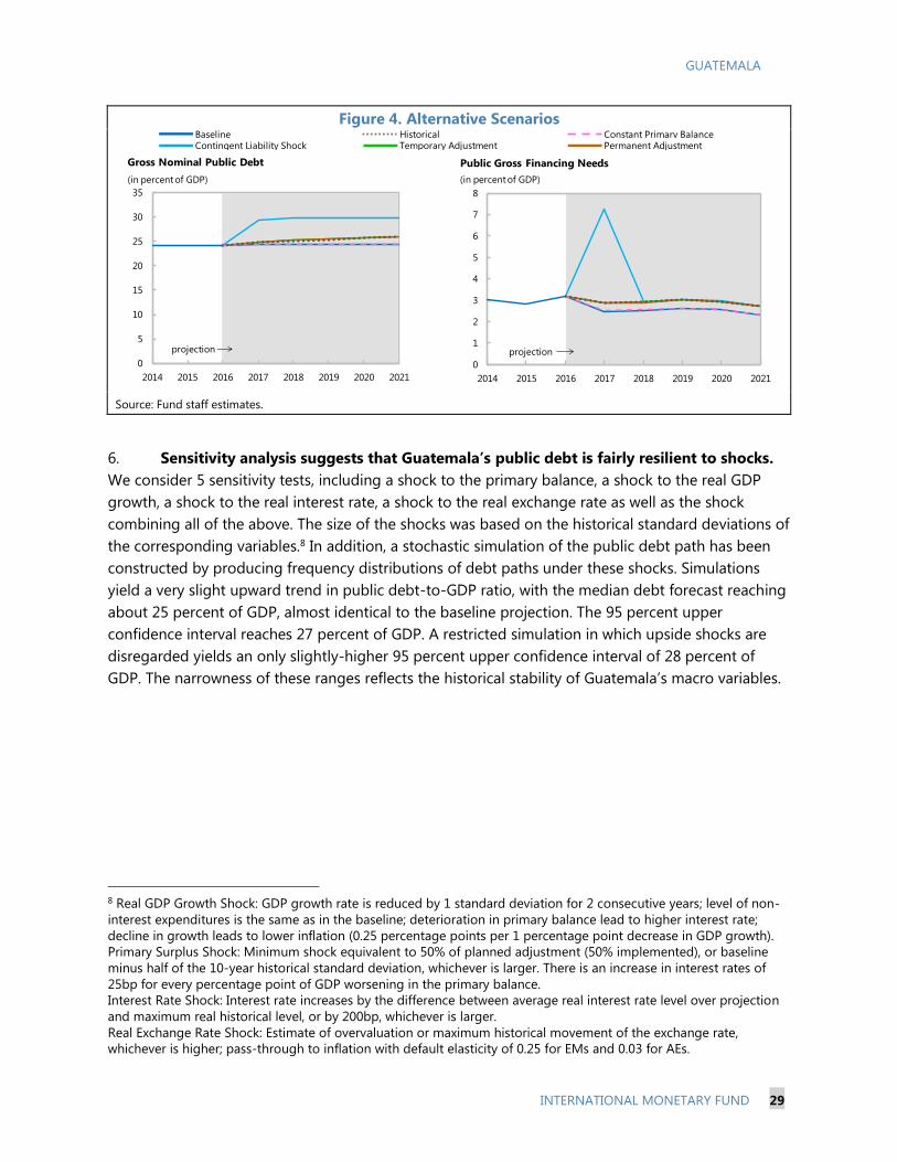
Figure 4. Alternative Scenarios
Source: Fund staff estimates.
6. Sensitivity analysis suggests that Guatemala’s public debt is fairly resilient to shocks.
We consider 5 sensitivity tests, including a shock to the primary balance, a shock to the real GDP
growth, a shock to the real interest rate, a shock to the real exchange rate as well as the shock
combining all of the above. The size of the shocks was based on the historical standard deviations of
the corresponding variables.8 In addition, a stochastic simulation of the public debt path has been
constructed by producing frequency distributions of debt paths under these shocks. Simulations
yield a very slight upward trend in public debt-to-GDP ratio, with the median debt forecast reaching
about 25 percent of GDP, almost identical to the baseline projection. The 95 percent upper
confidence interval reaches 27 percent of GDP. A restricted simulation in which upside shocks are
disregarded yields an only slightly-higher 95 percent upper confidence interval of 28 percent of
GDP. The narrowness of these ranges reflects the historical stability of Guatemala’s macro variables.
8 Real GDP Growth Shock: GDP growth rate is reduced by 1 standard deviation for 2 consecutive years; level of non-
interest expenditures is the same as in the baseline; deterioration in primary balance lead to higher interest rate;
decline in growth leads to lower inflation (0.25 percentage points per 1 percentage point decrease in GDP growth).
Primary Surplus Shock: Minimum shock equivalent to 50% of planned adjustment (50% implemented), or baseline
minus half of the 10-year historical standard deviation, whichever is larger. There is an increase in interest rates of
25bp for every percentage point of GDP worsening in the primary balance.
Interest Rate Shock: Interest rate increases by the difference between average real interest rate level over projection
and maximum real historical level, or by 200bp, whichever is larger.
Real Exchange Rate Shock: Estimate of overvaluation or maximum historical movement of the exchange rate,
whichever is higher; pass-through to inflation with default elasticity of 0.25 for EMs and 0.03 for AEs.
Contingent Liability Shock Temporary Adjustment Permanent AdjustmentBaseline Historical Constant Primary Balance
0
5
10
15
20
25
30
35
2014 2015 2016 2017 2018 2019 2020 2021
Gross Nominal Public Debt
(in percent of GDP)
projection
0
1
2
3
4
5
6
7
8
2014 2015 2016 2017 2018 2019 2020 2021
Public Gross Financing Needs
(in percent of GDP)
projection

GUATEMALA
30 INTERNATIONAL MONETARY FUND
Figure 6. Evolution of Predictive Densities of Gross Nominal Public Debt
(in percent of GDP)
Source: Fund staff estimates.
(in percent of GDP)
0
5
10
15
20
25
30
2014 2015 2016 2017 2018 2019 2020 2021
10th-25th 25th-75th 75th-90thPercentiles:Baseline
Symmetric Distribution
0
5
10
15
20
25
30
2014 2015 2016 2017 2018 2019 2020 2021
Restricted (Asymmetric) Distribution
no restriction on the growth rate shock
no restriction on the interest rate shock
0 is the max positive pb shock (percent GDP)
no restriction on the exchange rate shock
Restrictions on upside shocks:
Figure 5. Public DSA – Stress Tests
Source: Fund staff calculations.
Macro-Fiscal Stress Tests
Baseline Primary Balance Shock Real Interest Rate Shock
Real GDP Growth Shock Real Exchange Rate Shock
20
22
24
26
28
30
32
34
2016 2017 2018 2019 2020 2021
Gross Nominal Public Debt
(in percent of GDP)
200
210
220
230
240
250
260
270
2016 2017 2018 2019 2020 2021
Gross Nominal Public Debt
(in percent of Revenue)
Primary Balance Shock 2016 2017 2018 2019 2020 2021 Real GDP Growth Shock 2016 2017 2018 2019 2020 2021
Real GDP growth 3.8 3.7 3.8 3.8 3.9 4.0 Real GDP growth 3.8 2.7 2.7 3.8 3.9 4.0
Inflation 4.5 3.2 4.0 4.0 4.0 3.9 Inflation 4.5 3.0 3.7 4.0 4.0 3.9
Primary balance -0.1 -0.4 -0.4 -0.1 -0.1 -0.1 Primary balance -0.1 -0.3 -0.4 -0.1 -0.1 -0.1
Effective interest rate 6.6 6.6 6.6 6.6 6.6 6.6 Effective interest rate 6.6 6.6 6.6 6.6 6.6 6.6
Real Interest Rate Shock Real Exchange Rate Shock
Real GDP growth 3.8 3.7 3.8 3.8 3.9 4.0 Real GDP growth 3.8 3.7 3.8 3.8 3.9 4.0
Inflation 4.5 3.2 4.0 4.0 4.0 3.9 Inflation 4.5 4.4 4.0 4.0 4.0 3.9
Primary balance -0.1 -0.1 -0.1 -0.1 -0.1 -0.1 Primary balance -0.1 -0.1 -0.1 -0.1 -0.1 -0.1
Effective interest rate 6.6 6.6 6.8 7.0 7.2 7.3 Effective interest rate 6.6 6.8 6.6 6.6 6.6 6.5
(in percent)
Underlying Assumptions

GUATEMALA
INTERNATIONAL MONETARY FUND 31
7. While not an immediate concern, rising demographic pressures, if left unaddressed,
would pose challenges for the budget in the medium and long term. Pension spending in the
central government budget has generated a deficit of 0.41 percent of GDP in 2015 and is predicted
to rise slightly to 0.45 percent of GDP in 2016 under the baseline scenario. However, rising aging
pressures would likely lead to a somewhat higher central government pension spending in the
future (currently estimated at an additional ¼ percent of GDP). Given the history of deficit
containment, the baseline scenario assumes that these additional expenditure pressures would be
accommodated through budget cuts elsewhere, thereby likely reducing even further social and
infrastructure spending. In addition, actuarial projections suggest that the social security institute
(IGSS) will start running a deficit in 2017 and will deplete its reserves to cover the deficit by 2030.
While this rising pension deficit does not directly affect the central government budget, it represents
contingent liability for the government. Therefore, in the longer run a parametric reform (for
example, an increase in the pension age and contributions) of the pension system will be needed to
bring the pension system on a sustainable footing.
B. Poverty, Inequality and Fiscal Redistribution9
Guatemala has high levels of poverty and inequality, with distinct patterns in terms of
rural-urban as well as ethnic divide. At the same time, low tax revenues constrain the size
of the government and thus the scope to pursue social objectives. This section quantifies
the poverty gap in Guatemala and estimates the effect on growth and redistribution of
alternative tax/spending policy combinations. Results suggest that the extreme poverty
gap amounts to about 1 percent of 2016 GDP, while lifting all poor out of total poverty
would take at least 7 percent of GDP. Raising revenues through higher and more
progressive PIT would be less detrimental to growth and poverty/inequality than the VAT.
Redistributing 1 percent of GDP through the existing cash transfer program would reduce
extreme poverty by 4 percentage points. Trade-offs on the spending side imply that both
cash transfers and public investment need to increase in order to reduce poverty while
simultaneously fostering growth.
Trends in Poverty and Inequality
8. Poverty and inequality in Guatemala are high compared to regional peers. Contrary to
other countries in the region where poverty has decreased over time, both poverty and extreme
poverty have increased in Guatemala over the last decade. Poverty incidence also displays a clear
regional pattern and is significantly higher in rural compared to urban areas, which also translates in
a clear ethnic divide as indigenous populations mostly reside in rural regions. High extreme poverty
has dire consequences for basic nutrition outcomes, hence the higher incidence of malnutrition in
Guatemala compared to regional peers and other countries in the world.
9 Preparad by Valentina Flamini, Marina Mendez Tavares, Adrian Peralta-Alva, and Xuan Tam.

GUATEMALA
32 INTERNATIONAL MONETARY FUND
Figure 7. Poverty and Inequality Indicators
9. Persistently low tax revenue constrains the size of the budget and limit the
government’s capacity to pursue social objectives. At 10.2 percent of GDP in 2016, tax revenues
are among the lowest in the world, which limit the size of government and its spending capacity. As
a result, social spending is also very low, even compared to countries with similar per capita income
levels. Additionally, revenue to GDP ratios have been declining over the last few years, not least as a
consequence of the political crisis in 2015. Given the government’s prudent fiscal policy, spending
cuts have overcompensated for such declines and in particular public investment that has typically
absorbed the brunt of the fiscal adjustment.
0
0.2
0.4
0.6
0.8
1
0
10
20
30
40
50
60
70
80
90
CRI PAN AL6 DOM SLV NIC HND GTM
Poverty
Inequality (rhs)
Poverty and Inequality
(Percent of population below poverty line of $4/day;
and Gini coefficients)
56.451.2
59.3
15.7 15.3
23.4
0
10
20
30
40
50
60
2000 2006 2014
Total
Extreme
Poverty Rates
(Percent of Total Population)
0
10
20
30
40
50
60
70
80
90
Rural Indigenous Rural Indigenous
Poverty Rates
(Percent of Total Population, 2014)
Total Extreme
Urban
Non-Indigenous
0
10
20
30
40
50
60
Stunting Undernourishment Underweight
GTM
LA5
Malnutrition
(Percent of Total Population, 2014)

GUATEMALA
INTERNATIONAL MONETARY FUND 33
Figure 8. Revenue, Expenditure, and Social Spending
10. Hence, in 2014 more than 20 percent of the population lived in extreme poverty while
almost 60 percent were generally poor. The cumulative distribution of household per capita
consumption below, based on the released 2014 ENCOVI microdata, shows that the per capita
consumption of more than 20 percent of the population remained below the extreme poverty line
(first from the left) and was below the general poverty line (second from the left) for about
60 percent of the population. At the same time, the distribution of per capita consumption in the
second panel shows how most of the 40 percent of population confined between the two poverty
lines are clustered just above extreme poverty as showed by the mode of the distribution
approaching the extreme poverty line from the right. The third panel below presents annual
households per capita consumption in quetzales by consumption deciles: the consumption of the
first two and six deciles is lower than the extreme and general poverty lines respectively, consistently
with Guatemala’s extreme poverty rate of 23 and the general poverty rate of 59 percent.
Figure 9. Consumption Distribution
0
10
20
30
40
50
60
Revenue Expenditure
Guatemala
Median of Emerging and Developing countries
GTM
0
5
10
15
20
25
30
35
40
0 50 100
So
cial s
pend
ing
(%
of G
DP)
GDP per capita, PPP
Social Spending
(2013)
-1.4
-1.2
-1
-0.8
-0.6
-0.4
-0.2
0
0.2
0.4
0.6
2011 2012 2013 2014 2015
Revenue
Expenditure
Central Government Revenue and Expenditure
(Annual change, Percent of GDP)
-
10,000
20,000
30,000
40,000
1 2 3 4 5 6 7 8 9 10 Tot
Total Consumption
Poverty Line
Extreme Poverty Line
Consumption and Poverty by Income Decile
(Quetzales Per Capita, Per Year)
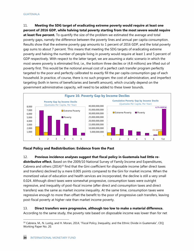
GUATEMALA
34 INTERNATIONAL MONETARY FUND
11. Meeting the SDG target of eradicating extreme poverty would require at least one
percent of 2016 GDP, while halving total poverty starting from the most severe would require
at least five percent. To quantify the size of the problem we estimated the average and total
poverty gaps, namely the difference between the poverty lines and annual per capita consumption.
Results show that the extreme poverty gap amounts to 1 percent of 2016 GDP, and the total poverty
gap sums to about 7 percent. This means that meeting the SDG targets of eradicating extreme
poverty and halving the number of people living in poverty would require at least 1 and 5 percent of
GDP respectively. With respect to the latter target, we are assuming a static scenario in which the
most severe poverty is eliminated first, i.e., the bottom three deciles or (4.8 millions) are lifted out of
poverty first. This would be the notional annual cost of a perfect cash transfer program perfectly
targeted to the poor and perfectly calibrated to exactly fill the per capita consumption gap of each
household. In practice, of course, there is no such program: the cost of administration, and imperfect
targeting (both in terms of beneficiaries and benefit amount), which crucially depend on the
government administrative capacity, will need to be added to these lower bounds.
Figure 10. Poverty Gap by Income Deciles
Fiscal Policy and Redistribution: Evidence from the Past
12. Previous incidence analyses suggest that fiscal policy in Guatemala had little re-
distributive effect. Based on the 2009/10 National Survey of Family Income and Expenditures,
Cabrera and others (2014)10 find that the Gini coefficient for disposable income (after direct taxes
and transfers) declined by a mere 0.005 points compared to the Gini for market income. When the
monetized value of education and health services are incorporated, the decline is still a very small
0.024. Although direct taxes were somewhat progressive, consumption taxes were outright
regressive, and inequality of post-fiscal income (after direct and consumption taxes and direct
transfers) was the same as market income inequality. At the same time, consumption taxes were
regressive enough to more than offset the benefit to the poor of progressive cash transfers, leaving
post-fiscal poverty at higher rate than market income poverty.
13. Direct transfers were progressive, although too low to make a material difference.
According to the same study, the poverty rate based on disposable income was lower than for net
10 Cabrera, M., N. Lustig, and H. Moran, 2014, “Fiscal Policy, Inequality, and the Ethnic Divide in Guatemala”, CEQ
Working Paper No. 20.
-
1,000
2,000
3,000
4,000
5,000
6,000
7,000
8,000
1 2 3 4 5 6
Extreme Poverty
Poverty
Poverty Gap by Income Decile
(Quetzales Per Capita, Per Year)
-
5,000,000,000
10,000,000,000
15,000,000,000
20,000,000,000
25,000,000,000
30,000,000,000
35,000,000,000
40,000,000,000
1 2 3 4 5 6 Tot
Extreme Poverty Poverty
Cumulative Poverty Gap by Income Decile
(Quetzales Per Capita, Per Year)
1% GDP16
6.7% GDP16
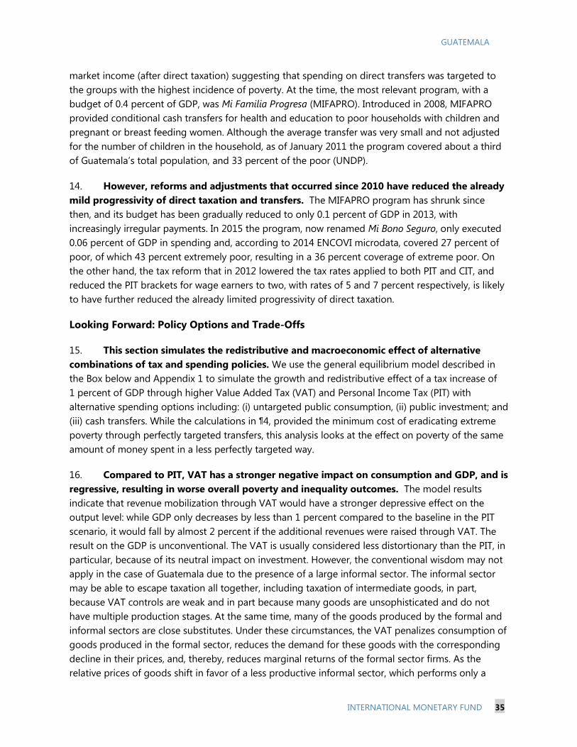
GUATEMALA
INTERNATIONAL MONETARY FUND 35
market income (after direct taxation) suggesting that spending on direct transfers was targeted to
the groups with the highest incidence of poverty. At the time, the most relevant program, with a
budget of 0.4 percent of GDP, was Mi Familia Progresa (MIFAPRO). Introduced in 2008, MIFAPRO
provided conditional cash transfers for health and education to poor households with children and
pregnant or breast feeding women. Although the average transfer was very small and not adjusted
for the number of children in the household, as of January 2011 the program covered about a third
of Guatemala’s total population, and 33 percent of the poor (UNDP).
14. However, reforms and adjustments that occurred since 2010 have reduced the already
mild progressivity of direct taxation and transfers. The MIFAPRO program has shrunk since
then, and its budget has been gradually reduced to only 0.1 percent of GDP in 2013, with
increasingly irregular payments. In 2015 the program, now renamed Mi Bono Seguro, only executed
0.06 percent of GDP in spending and, according to 2014 ENCOVI microdata, covered 27 percent of
poor, of which 43 percent extremely poor, resulting in a 36 percent coverage of extreme poor. On
the other hand, the tax reform that in 2012 lowered the tax rates applied to both PIT and CIT, and
reduced the PIT brackets for wage earners to two, with rates of 5 and 7 percent respectively, is likely
to have further reduced the already limited progressivity of direct taxation.
Looking Forward: Policy Options and Trade-Offs
15. This section simulates the redistributive and macroeconomic effect of alternative
combinations of tax and spending policies. We use the general equilibrium model described in
the Box below and Appendix 1 to simulate the growth and redistributive effect of a tax increase of
1 percent of GDP through higher Value Added Tax (VAT) and Personal Income Tax (PIT) with
alternative spending options including: (i) untargeted public consumption, (ii) public investment; and
(iii) cash transfers. While the calculations in ¶4, provided the minimum cost of eradicating extreme
poverty through perfectly targeted transfers, this analysis looks at the effect on poverty of the same
amount of money spent in a less perfectly targeted way.
16. Compared to PIT, VAT has a stronger negative impact on consumption and GDP, and is
regressive, resulting in worse overall poverty and inequality outcomes. The model results
indicate that revenue mobilization through VAT would have a stronger depressive effect on the
output level: while GDP only decreases by less than 1 percent compared to the baseline in the PIT
scenario, it would fall by almost 2 percent if the additional revenues were raised through VAT. The
result on the GDP is unconventional. The VAT is usually considered less distortionary than the PIT, in
particular, because of its neutral impact on investment. However, the conventional wisdom may not
apply in the case of Guatemala due to the presence of a large informal sector. The informal sector
may be able to escape taxation all together, including taxation of intermediate goods, in part,
because VAT controls are weak and in part because many goods are unsophisticated and do not
have multiple production stages. At the same time, many of the goods produced by the formal and
informal sectors are close substitutes. Under these circumstances, the VAT penalizes consumption of
goods produced in the formal sector, reduces the demand for these goods with the corresponding
decline in their prices, and, thereby, reduces marginal returns of the formal sector firms. As the
relative prices of goods shift in favor of a less productive informal sector, which performs only a

GUATEMALA
36 INTERNATIONAL MONETARY FUND
small part of investment in the economy (the majority is done by the formal sector), the VAT
becomes distortive both in terms of consumption allocations and in terms of investment decisions.
Hence, while the PIT is always distortive with or without the informal sector, the VAT can become
distortive in the presence of the informal sector. This, however, does not automatically guarantee
that the VAT has to be more distortive than the PIT. It is the particular structure of the PIT in
Guatemala with extremely low rates and little progressivity and a relatively high VAT rate that help
explain the result.11 At the same time, VAT is regressive, thus poverty and inequality increase more.
11 An empirical study by Acosta-Ormaechea and Yoo (2012) also finds that in low income countries PIT does not
significantly affect growth, likely due to the low level of PIT collection in such countries (1.5 percent of GDP on
average). This result is relevant for Guatemala where PIT collection is only 0.4 percent of GDP.
0
5
10
15
20
25
30
35
40
45
GTM
PR
Y
BO
L
PA
N
CR
I
ATG
HN
D
TTO
JAM
DO
M
BR
A
SLV
NIC
LCA
GU
Y
PER
UR
Y
VC
T
CO
L
VEN
EC
U
DM
A
MEX
BR
B
AR
G
CH
L
EM Average
LAC: PIT Rates, 2015
(Percent)
0
5
10
15
20
25
PA
N
BH
S
PR
Y
EC
U
GTM
VEN
CR
I
SLV
BO
L
ATG
DM
A
HN
D
NIC
LCA
VC
T
TTO
CO
L
GU
Y
MEX
PER
JAM
KN
A
BR
B
DO
M
BR
A
CH
L
AR
G
UR
Y
EM Average
LAC: VAT Rates, 2015
(Percent)

GUATEMALA
INTERNATIONAL MONETARY FUND 37
Box 1. General Structure of the Model
Small open economy with three consumption goods: agricultural, services, and manufacturing and
modern services.1
There are four types of households: two types in the urban area: skilled and unskilled urban; and two
types in the rural area small-land holders, and large-land holders. Within each of the first three types, there is a
continuum of households, equal ex ante, but facing idiosyncratic risk. Households solve dynamic optimization
problems taking prices and government policies as given. Households receive remittances in a lump-sum fashion,
their magnitude and distribution match the data.
Four goods are produced: (i) agricultural commodities for exports (and not domestically consumed), (ii)
agricultural goods for domestic consumption (non-tradable), (iii) manufacturing (tradable), and (iv) services (non-
tradable).
The only financial assets available are one-period capital share holdings. The total amount of capital
shareholdings equals the capital stock of the manufacturing sector. These titles are traded among households to
allow for risk sharing. The interest rate of these assets and the price of domestic food are determined by supply
and demand forces in equilibrium.
The government collects tax revenue (on income, consumption, etc.). This revenue is used to fund
government expenditures (including public sector wages, capital investment and other pro-poor spending).
The model is thus a dynamic general equilibrium including a continuum of households facing
idiosyncratic risk (as in the income inequality literature) and also multiple sectors (as in the structural
transformation literature).
1 Manufacturing should be understood as the modern, high productivity sector of the economy (and thus include
some services like banking, finance, etc.; while services refer to the informal non-taxable activities, such as personal
services.
Figure 11. Impact of VAT and PIT Increases on Economic Activity, Poverty, and Inequality
17. Spending in untargeted government consumption would result in a contraction of
growth as the distortive effect of taxation would prevail. Given its superior growth and
distributional outcomes, we focus on PIT increases for the analysis of spending scenarios. If the
additional revenue was used to finance untargeted government consumption, GDP would shrink
following the reduction in private consumption and investment. In addition, since government
-3
-2
-1
0
1
2
GDP C I G X
Value Added Tax
Personal Income Tax
Economic Activity
(Percentage change from baseline)
0
2
4
6
8
10
12
14
Personal Income Tax
Value Added Tax
Personal Income Tax
Value Added Tax
Poverty Extreme Poverty
Poverty and Extreme Poverty
(Percentage change from baseline)
-0.8
-0.7
-0.6
-0.5
-0.4
-0.3
-0.2
-0.1
0.0
Personal Income Tax Value Added Tax
Inequality: Gini Coefficient
(Percentage change from baseline)
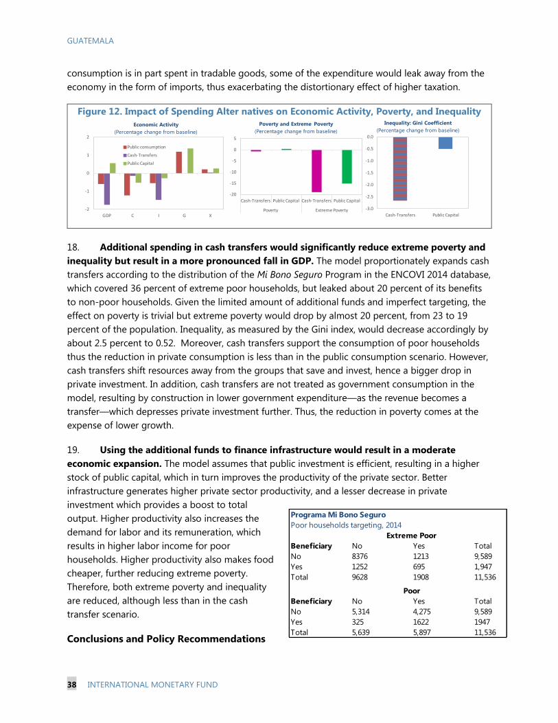
GUATEMALA
38 INTERNATIONAL MONETARY FUND
consumption is in part spent in tradable goods, some of the expenditure would leak away from the
economy in the form of imports, thus exacerbating the distortionary effect of higher taxation.
Figure 12. Impact of Spending Alter natives on Economic Activity, Poverty, and Inequality
18. Additional spending in cash transfers would significantly reduce extreme poverty and
inequality but result in a more pronounced fall in GDP. The model proportionately expands cash
transfers according to the distribution of the Mi Bono Seguro Program in the ENCOVI 2014 database,
which covered 36 percent of extreme poor households, but leaked about 20 percent of its benefits
to non-poor households. Given the limited amount of additional funds and imperfect targeting, the
effect on poverty is trivial but extreme poverty would drop by almost 20 percent, from 23 to 19
percent of the population. Inequality, as measured by the Gini index, would decrease accordingly by
about 2.5 percent to 0.52. Moreover, cash transfers support the consumption of poor households
thus the reduction in private consumption is less than in the public consumption scenario. However,
cash transfers shift resources away from the groups that save and invest, hence a bigger drop in
private investment. In addition, cash transfers are not treated as government consumption in the
model, resulting by construction in lower government expenditure—as the revenue becomes a
transfer—which depresses private investment further. Thus, the reduction in poverty comes at the
expense of lower growth.
19. Using the additional funds to finance infrastructure would result in a moderate
economic expansion. The model assumes that public investment is efficient, resulting in a higher
stock of public capital, which in turn improves the productivity of the private sector. Better
infrastructure generates higher private sector productivity, and a lesser decrease in private
investment which provides a boost to total
output. Higher productivity also increases the
demand for labor and its remuneration, which
results in higher labor income for poor
households. Higher productivity also makes food
cheaper, further reducing extreme poverty.
Therefore, both extreme poverty and inequality
are reduced, although less than in the cash
transfer scenario.
Conclusions and Policy Recommendations
-3.0
-2.5
-2.0
-1.5
-1.0
-0.5
0.0
Cash-Transfers Public Capital
Inequality: Gini Coefficient
(Percentage change from baseline)
-2
-1
0
1
2
GDP C I G X
Public consumption
Cash-Transfers
Public Capital
Economic Activity
(Percentage change from baseline)
-20
-15
-10
-5
0
5
Cash-Transfers Public Capital Cash-Transfers Public Capital
Poverty Extreme Poverty
Poverty and Extreme Poverty
(Percentage change from baseline)
Programa Mi Bono Seguro
Poor households targeting, 2014
Beneficiary No Yes Total
No 8376 1213 9,589
Yes 1252 695 1,947
Total 9628 1908 11,536
Beneficiary No Yes Total
No 5,314 4,275 9,589
Yes 325 1622 1947
Total 5,639 5,897 11,536
Extreme Poor
Poor

GUATEMALA
INTERNATIONAL MONETARY FUND 39
20. Mobilizing tax revenues is crucial to achieve social objectives. The government of
Guatemala needs tax revenues to improve social conditions and lift its people out of extreme
poverty and malnutrition. While in the short term revenue administration measures to widen the tax
base should be prioritized, in the medium to long term—once the taxpayers’ morale is restored—tax
rates increases are likely to be needed. In this respect, improving the collection of VAT will be key,
and so would be making the PIT regime more progressive. Our results show that eradicating
extreme poverty would require at least 1 percent of GDP.
21. The way resources are mobilized and spent matters. Alternative taxes and spending
strategies have different outcomes in terms of macroeconomic impact and redistribution, hence a
careful analysis of growth and poverty effects is required when designing tax/spending policies. Our
analysis suggests that, likely due to its current low rates and relatively neutral structure, PIT would
generate a larger reducing effect on inequality and less distortionary impact on growth. Design, of
course, matters too, and any identified policy measure can be designed to mitigate the negative
effect on growth and the poor.
22. When it comes to spending, there are trade-offs between growth and redistribution
objectives. While cash transfers are more efficient in reducing extreme poverty and inequality,
(efficient) public investment generates better growth outcomes. Hence, both government transfers
and public investment will need to rise to spur growth and reduce poverty and inequality. Our
results suggest that expanding existing CCT programs by 1 percent of GDP to increase benefits
would reduce the extreme poverty rate from 23 to 19 percent. However, growth and social
objectives do not need to be incompatible if a virtuous cycle can be started where economic growth
improves the living condition of people and a less poor, more productive labor force contributes to
faster economic growth. In this respect, effective targeting and efficient public investment spending
are key to maximize the social and growth returns of higher tax yields.

GUATEMALA
40 INTERNATIONAL MONETARY FUND
References
Davies, A. “Human Development and the Optimal Size of Government,” Journal of Socioeconomics,
2009, Vol. 35, No. 5, pp. 868–76.
Gunalp, B. and Dincer, O., 2005, “The Optimal Government Size in Transition Countries,” Department
of Economics, Hacettepe University Beytepe, Ankara and Department of Commerce, Massey
University, Auckland
Karras, G., 1997, “On the Optimal Government Size in Europe: Theory and Empirical Evidence,” The
Manchester School of Economic & Social Studies
Peden, E., 1991, “Productivity in the United States and its relationship to government activity: An
analysis of 57 years, 1929–1986.”
GUATEMALA
INTERNATIONAL MONETARY FUND 41
Appendix. Model Details1
We consider a small open economy populated by a continuum of heterogeneous households who
live indefinitely and face idiosyncratic shocks. All types of households have the same preferences
over the consumption of food, 𝑐𝑓, manufacturing 𝑐𝑚, and services, 𝑐𝑠. We assume that services
are non-tradable, while manufacturing and food is tradable, and also the numeraire.
There are three fixed types of households in the model: large farmers, rural households, and urban
households. Rural households own a small plot of land and have the occupational choice problem of
choosing the amount time to devote to producing food (which requires labor and land), and the
amount of time working for large farmers for a competitive wage 𝑤𝑟. Similarly, urban households
have the occupational choice problem of choosing the optimal amount of time to produce services
(which use only labor as an input), and how much time to work in manufacturing for a competitive
wage 𝑤. We assume that households cannot move across rural and urban sectors.
Large farmers own a large plot of land where they can produce food for the domestic market or
exports. They hire labor from small farmers and also accumulate capital, both of which are used to
produce agricultural goods for export. Large farmers’ capital follows a standard law of motion of
capital:
𝑘+𝑓
= 𝑥𝑓 + (1 − δ)𝑘𝑓
Finally, there are competitive firms that produce manufacturing goods using capital and labor as an
input. Manufacturing can also be used indistinctly for investment by large farmers or for
consumption. Markets are incomplete, urban and rural households can save at a risk-free interest
rate 𝑟. Entrepreneurs can borrow at a rate (1 + 𝑑)𝑟, where 𝑑 captures the risk premium in lending.
We assume that the capital account is closed and trade balance is always zero.
The government collects value added taxes on food 𝜏𝑎 and manufacturing goods 𝑟𝑚, trade taxes
𝑟∗, corporate taxes 𝜏𝑓, and labor income taxes 𝜏𝑤. The government spends part of its resources on
manufacturing goods, and gives or collects lump-sum taxes that may be specific to each household
type. In the next section we explain the urban households’ problem.
The framework considered here is a continuum of infinitely-lived agents with productivity risk. The
model is small open economy with three different agents types: urban households 𝑢, farms 𝑓, and
rural households 𝑟. The total mass of agents is normalized to equal 1. All agents maximize the
present value of their consumption over three different types of goods: food 𝑐𝑎, manufactured
goods 𝑐𝑚, and services 𝑐𝑠.
1 This application is part of a research project on macroeconomic policy supported by the U.K.’s Department for
International Development (DFID) but should not be reported as representing the views of DFID.
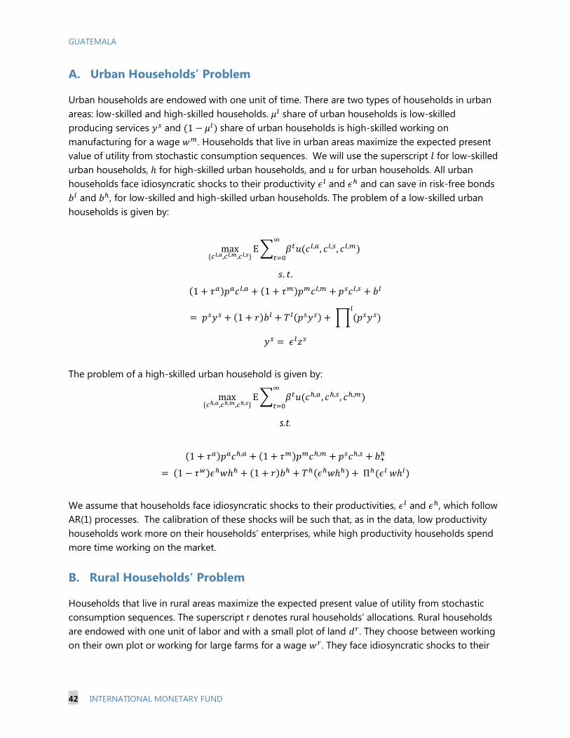
GUATEMALA
42 INTERNATIONAL MONETARY FUND
A. Urban Households’ Problem
Urban households are endowed with one unit of time. There are two types of households in urban
areas: low-skilled and high-skilled households. 𝜇𝑙 share of urban households is low-skilled
producing services 𝑦𝑠 and (1 − 𝜇𝑙) share of urban households is high-skilled working on
manufacturing for a wage 𝑤𝑚. Households that live in urban areas maximize the expected present
value of utility from stochastic consumption sequences. We will use the superscript 𝑙 for low-skilled
urban households, ℎ for high-skilled urban households, and 𝑢 for urban households. All urban
households face idiosyncratic shocks to their productivity 𝜖𝑙 and 𝜖ℎ and can save in risk-free bonds
𝑏𝑙 and 𝑏ℎ, for low-skilled and high-skilled urban households. The problem of a low-skilled urban
households is given by:
max{𝑐𝑙,𝑎,𝑐𝑙,𝑚,𝑐𝑙,𝑠}
E ∑ 𝛽𝑡𝑢(𝑐𝑙,𝑎 , 𝑐𝑙,𝑠, 𝑐𝑙,𝑚)∞
𝑡=0
𝑠. 𝑡.
(1 + 𝜏𝑎)𝑝𝑎𝑐𝑙,𝑎 + (1 + 𝜏𝑚)𝑝𝑚𝑐𝑙,𝑚 + 𝑝𝑠𝑐𝑙,𝑠 + 𝑏𝑙
= 𝑝𝑠𝑦𝑠 + (1 + 𝑟)𝑏𝑙 + 𝑇𝑙(𝑝𝑠𝑦𝑠) + ∏ (𝑝𝑠𝑦𝑠)𝑙
𝑦𝑠 = 𝜖𝑙𝑧𝑠
The problem of a high-skilled urban household is given by:
max{𝑐ℎ,𝑎,𝑐ℎ,𝑚,𝑐ℎ,𝑠}
E ∑ 𝛽𝑡𝑢(𝑐ℎ,𝑎 , 𝑐ℎ,𝑠, 𝑐ℎ,𝑚)∞
𝑡=0
s.t.
(1 + 𝜏𝑎)𝑝𝑎𝑐ℎ,𝑎 + (1 + 𝜏𝑚)𝑝𝑚𝑐ℎ,𝑚 + 𝑝𝑠𝑐ℎ,𝑠 + 𝑏+ℎ
= (1 − 𝜏𝑤)𝜖ℎ𝑤ℎℎ + (1 + 𝑟)𝑏ℎ + 𝑇ℎ(𝜖ℎ𝑤ℎℎ) + Πℎ(𝜖𝑙 𝑤ℎ𝑙)
We assume that households face idiosyncratic shocks to their productivities, 𝜖𝑙 and 𝜖ℎ, which follow
AR(1) processes. The calibration of these shocks will be such that, as in the data, low productivity
households work more on their households’ enterprises, while high productivity households spend
more time working on the market.
B. Rural Households’ Problem
Households that live in rural areas maximize the expected present value of utility from stochastic
consumption sequences. The superscript r denotes rural households’ allocations. Rural households
are endowed with one unit of labor and with a small plot of land 𝑑𝑟. They choose between working
on their own plot or working for large farms for a wage 𝑤𝑟. They face idiosyncratic shocks to their

GUATEMALA
INTERNATIONAL MONETARY FUND 43
productivity on their own plot and can save in a risk-free bond 𝑏𝑟. The maximization problem of a
rural household is given by:
max{𝑐𝑢,𝑎,𝑐𝑢,𝑚,𝑐𝑟,𝑠,ℎ𝑢}
E ∑ 𝛽𝑡𝑢(𝑐𝑟,𝑎 , 𝑐𝑟,𝑠, 𝑐𝑟,𝑚)∞
𝑡=0
s.t.
(1 + 𝜏𝑎)𝑝𝑎𝑐𝑟,𝑎 + (1 + 𝜏𝑚)𝑝𝑚𝑐𝑟,𝑚 + 𝑝𝑠𝑐𝑟,𝑠 + 𝑏𝑟
= (1 − 𝜏𝑤)𝜖𝑟𝑤𝑓ℎ𝑟 + 𝑝𝑎𝑦𝑎 + (1 + 𝑟)𝑏𝑟 + 𝑇𝑟(𝜖ℎ𝑤𝑓ℎ𝑓) + ∏ (𝜖𝑟𝑤𝑓ℎ𝑓)𝑟
𝑦𝑎 = 𝑧𝑎𝜖𝑟(𝑑𝑟)𝛼𝑎(1 − ℎ𝑟)1−𝛼𝑎
ℎ𝑟 ∈ [0,1]
We assume that households face idiosyncratic shocks to their productivity, 𝜖𝑟 follows an AR(1)
process. The calibration of these shocks will be such that as in the data, low productivity households
devote the majority of their time working for big farms, while high productivity households spend
more time working on their own farms.
C. Large Farm’s Problem
Farmers that own larger plots of land also maximize their present discounted utility. They do not
face any idiosyncratic risk, and the economy is assumed to be in a stationary state so that prices are
constant through time. Hence, they do no face any uncertainty. Large farmers produce two goods
domestic food and exports. The production of exports requires land 𝑑∗, capital 𝑘𝑓 and labor ℎ∗,
while the production of food only requires land 𝑑𝑎 and labor ℎ𝑎. We assume that there is no land
market, and consequently the allocation of land between domestic and export goods is fixed. Large
farmers choose how much labor to hire to produce for the domestic and the external markets, and
how much capital to accumulate. The problem of a larger farmer is given by:
max{𝑐𝑓,𝑎,𝑐𝑓,𝑚,𝑐𝑓,𝑠,𝑘+
𝑓,ℎ𝑎,ℎ∗}
E ∑ 𝛽𝑡𝑢(𝑐𝑓,𝑎 , 𝑐𝑓,𝑠, 𝑐𝑓,𝑚)∞
𝑡=0
s.t.
(1 + 𝜏𝑎)𝑝𝑎𝑐𝑓,𝑎 + (1 + 𝜏𝑚)𝑝𝑚𝑐𝑓,𝑚 + 𝑝𝑠𝑐𝑓,𝑠 + 𝑝𝑚𝑘𝑓
= 𝑌∗ + 𝜏∗𝛿𝑝𝑚𝑘𝑓 + (1 − 𝛿)𝑝𝑚𝑘𝑓 + 𝑇𝑓(𝑌∗) + ∏ (𝑌∗)𝑓
𝜋𝑎 = 𝑝𝑎𝑧𝑎(𝑑)𝛼1𝑎
(ℎ𝑎)1−𝛼1𝑎
− 𝑤𝑓ℎ𝑎
𝜋∗ = 𝑝∗𝑧(𝑑∗)𝛼1∗(ℎ∗)𝛼2
∗(𝑘𝑓)(1−𝛼1
∗−𝑎2∗ ) − 𝑤𝑓ℎ𝑎
𝑌∗ = (1 − 𝜏𝑟)𝜋𝑎 + (1 − 𝜏∗)𝜋∗
ℎ𝑎 , ℎ∗ ≥ 0
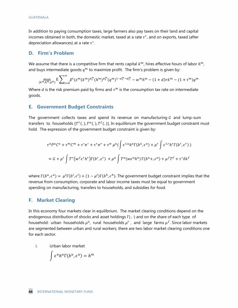
GUATEMALA
44 INTERNATIONAL MONETARY FUND
In addition to paying consumption taxes, large farmers also pay taxes on their land and capital
incomes obtained in both, the domestic market, taxed at a rate 𝜏𝑟, and on exports, taxed (after
depreciation allowances) at a rate 𝜏∗.
D. Firm’s Problem
We assume that there is a competitive firm that rents capital 𝑘𝑚, hires effective hours of labor ℎ𝑚,
and buys intermediate goods 𝑞𝑚 to maximize profit. The firm’s problem is given by:
max{𝑘𝑚,ℎ𝑚,𝑞𝑚}
E ∑ 𝛽𝑡(𝑧𝑚(𝑘𝑚)𝛼1𝑚
(ℎ𝑚)𝛼2𝑚
(𝑞𝑚)1−𝛼1𝑚−𝛼2
𝑚− 𝑤𝑚ℎ𝑚 − (1 + 𝑑)𝑟𝑘𝑚 − (1 + 𝜏𝑚)𝑞𝑚
∞
𝑡=0
Where 𝑑 is the risk premium paid by firms and 𝜏𝑚 is the consumption tax rate on intermediate
goods.
E. Government Budget Constraints
The government collects taxes and spend its revenue on manufacturing 𝐺 and lump-sum
transfers to households {𝑇𝑟(. ), 𝑇𝑢(. ), 𝑇𝑓(. )}. In equilibrium the government budget constraint must
hold. The expression of the government budget constraint is given by:
𝜏𝑎𝑃𝑎𝐶𝑎 + 𝜏𝑚𝐶𝑚 + 𝜏∗𝜋∗ + 𝜏𝑟𝜋𝑟 + 𝜏𝑤 𝜇𝑢(∫ 𝜖1,𝑢ℎ𝑢Γ(𝑏𝑢, 𝜖𝑢) + 𝜇𝑟 ∫ 𝜖1,𝑟ℎ𝑟Γ(𝑏𝑟 , 𝜖𝑟) )
= 𝐺 + 𝜇𝑟 ∫ 𝑇𝑟(𝑤𝑓𝜖𝑟ℎ𝑟)Γ(𝑏𝑟 , 𝜖𝑟) + 𝜇𝑢 ∫ 𝑇𝑢(𝑤𝜖𝑢ℎ𝑢) Γ(𝑏𝑢+, 𝜖𝑢) + 𝜇𝑓𝑇𝑓 + 𝜏∗𝛿𝑘𝑓
where Γ(𝑏𝑢, 𝜖𝑢) = 𝜇𝑙Γ(𝑏𝑙 , 𝜖𝑙) + (1 − 𝜇𝑙)Γ(𝑏ℎ, 𝜖ℎ). The government budget constraint implies that the
revenue from consumption, corporate and labor income taxes must be equal to government
spending on manufacturing, transfers to households, and subsidies for food.
F. Market Clearing
In this economy four markets clear in equilibrium. The market clearing conditions depend on the
endogenous distribution of shocks and asset holdings Γ(·, ·) and on the share of each type of
household: urban households 𝜇𝑢, rural households 𝜇𝑟 , and large farms 𝜇𝑓. Since labor markets
are segmented between urban and rural workers, there are two labor market clearing conditions one
for each sector.
i. Urban labor market
∫ 𝜖𝑢ℎ𝑢Γ(𝑏𝑢, 𝜖𝑢) = ℎ𝑚

GUATEMALA
INTERNATIONAL MONETARY FUND 45
ii. Rural labor market
𝜇𝑟 ∫ 𝜖𝑟ℎ𝑟Γ(𝑏𝑟 , 𝜖𝑟) = 𝜇 𝑓(ℎ𝑎 + ℎ∗)
Interest rates must clear the capital market so that households’ savings are equal to the
capital demanded by manufacturing firms.
iii. Capital market
𝑘𝑚 = 𝜇𝑢 ∫ 𝑏𝑢Γ(𝑏𝑢, 𝜖𝑢) + 𝜇𝑟 ∫ 𝑏𝑟Γ(𝑏𝑟 , 𝜖𝑟)
Finally, the relative price of services and food must be such that the corresponding markets of
such non-tradable goods clear.
iv. Services market
𝜇𝑢 ∫ 𝑐𝑢,𝑠Γ(𝑏𝑢, 𝜖𝑢) + 𝜇𝑟 ∫ 𝑐𝑟,𝑠Γ(𝑏𝑟 , 𝜖𝑟) + 𝜇 𝑓𝑐𝑓,𝑠 = 𝜇𝑢 ∫ 𝜖𝑢𝑧𝑠(1 − ℎ𝑢)𝛼Γ(𝑏𝑢, 𝜖𝑢)
v. Food market
𝜇𝑢 ∫ 𝑐𝑢,𝑎Γ(𝑏𝑢, 𝜖𝑢) + 𝜇𝑟 ∫ 𝑐𝑟,𝑎Γ(𝑏𝑟, 𝜖𝑟) + 𝜇 𝑓𝑐𝑓,𝑎
= 𝜇𝑢 ∫ 𝜖𝑢𝑧𝑎(1 − ℎ𝑟)1−𝛼𝛼Γ(𝑏𝑢, 𝜖𝑢) + 𝜇 𝑓𝑧𝛼(𝑑𝛼)𝛼1
𝛼(ℎ𝛼)1−𝛼1
𝛼
G. Stationary Equilibrium
A competitive equilibrium for this economy is constituted by a stationary distribution of assets
holdings and idiosyncratic shocks {Γ}, sequences of service and agricultural prices, manufacturing
and rural wages, and interest rates {𝑝𝑠, 𝑝𝑎 , 𝑤𝑟 , 𝑤𝑓, 𝑟}, together with allocations of consumption,
investment, time use and bond holdings for each type of households, such that—given
manufacturing prices and exported goods prices {𝑝𝑚, 𝑝∗}, sectoral productivity, idiosyncratic shocks,
government spending, and predetermined taxes {𝜏𝑚, 𝜏𝑎 , 𝜏𝑤 , 𝜏𝑓 , 𝜏∗} and transfers {𝑇𝑟 , 𝑇𝑢, 𝑇𝑓}—the
stochastic sequence of allocations solve their respective constrained optimization problem, clear
markets, and satisfy the government budget constraint. Note that the market clearing conditions
along with the fact that the government and individual budgets constraints hold at every period,
imply that the external sector condition of a balanced current account is also satisfied (Walras’ law).
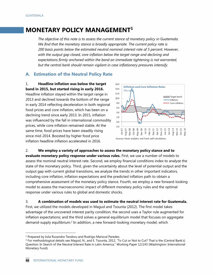
GUATEMALA
46 INTERNATIONAL MONETARY FUND
MONETARY POLICY MANAGEMENT1
The objective of this note is to assess the current stance of monetary policy in Guatemala.
We find that the monetary stance is broadly appropriate. The current policy rate is
200 basis points below the estimated neutral nominal interest rate of 5 percent. However,
with the output gap closed, core inflation below the target range and declining and
expectations firmly anchored within the band an immediate tightening is not warranted,
but the central bank should remain vigilant in case inflationary pressures intensify.
A. Estimation of the Neutral Policy Rate
1. Headline inflation was below the target
band in 2015, but started rising in early 2016.
Headline inflation stayed within the target range in
2013 and declined towards the bottom of the range
in early 2014 reflecting deceleration in both regional
food prices and core inflation, which has been on a
declining trend since early 2013. In 2015, inflation
was influenced by the fall in international commodity
prices, while core inflation remained stable. At the
same time, food prices have been steadily rising
since mid-2014. Boosted by higher food price
inflation headline inflation accelerated in 2016.
2. We employ a variety of approaches to assess the monetary policy stance and to
evaluate monetary policy response under various rules. First, we use a number of models to
assess the nominal neutral interest rate. Second, we employ financial conditions index to analyze the
state of the monetary policy. Third, given the uncertainty about the level of potential output and the
output gap with current global transitions, we analyze the trends in other important indicators,
including core inflation, inflation expectations and the predicted inflation path to obtain a
comprehensive assessment of the monetary policy stance. Fourth, we employ a new forward-looking
model to assess the macroeconomic impact of different monetary policy rules and the optimal
response under various rules to global and domestic shocks.
3. A combination of models was used to estimate the neutral interest rate for Guatemala.
First, we utilized the models developed in Magud and Tsounta (2012). The first model takes
advantage of the uncovered interest parity condition; the second uses a Taylor rule augmented for
inflation expectations; and the third solves a general equilibrium model that focuses on aggregate
demand-supply equilibrium.2 In addition, a new forward-looking monetary model, which
1 Prepared by Iulia Ruxandra Teodoru and Rodrigo Mariscal Paredes. 2 For methodological details see Magud, N., and E. Tsounta, 2012, “To Cut or Not to Cut? That is the (Central Bank’s)
Question: In Search of the Neutral Interest Rate in Latin America,” Working Paper 12/243 (Washington: International
Monetary Fund).
-2.0
0.0
2.0
4.0
6.0
8.0
10.0
12.0
14.0
16.0
Jan-0
7
Aug
-07
Mar-
08
Oct
-08
May-
09
Dec-
09
Jul-
10
Feb
-11
Sep
-11
Apr-
12
No
v-12
Jun
-13
Jan-1
4
Aug
-14
Mar-
15
Oct
-15
May-
16
Target band
Inflation
Core inflation
Inflation and Core Inflation Rates
(Percent)
Sources: Haver analytics and Fund staff calculations.

GUATEMALA
INTERNATIONAL MONETARY FUND 47
incorporates a New Keynesian Philips curve with international oil prices, an uncovered interest parity
condition, a forward-looking IS curve with real exchange rate and foreign demand, and a standard
Taylor rule, was developed. The model was employed not only to estimate the neutral monetary
policy rate but also to assess the optimal response to various shocks under the different monetary
policy rules. Estimation in all the models was based on a period 2001–2015. Looking at the
difference between the actual policy rate and the estimated neutral rate, an assessment of the
monetary stance can be made taking into account the economy’s current position in the cycle.
4. According to the average of the model estimates, the neutral nominal interest rate is
200 basis points above the actual nominal policy rate. With the output gap closed and inflation
projected to be within the target range in 2016, the estimates below suggest that the current policy
rate of 3 percent implies an accommodative monetary stance (Table 1). However, these results need
to be interpreted with caution, given the limitations of the data, the incipient nature of financial
markets in Guatemala, and the uncertainty about potential output and the output gap in the global
economy and in Guatemala, in particular.
Table 1. Neutral Real Interest Rate for Guatemala
5. The uncovered interest parity condition (UIPC) suggests the neutral nominal interest
rate of 5.6 percent. This value of 5.6 percent assumes an implicit annual nominal depreciation in
line with the inflation differential with the U.S. to maintain the real exchange rate constant, and takes
into account the country’s risk premium (e.g. EMBI spread). The “model” comprises the following
equations:
* ˆt ti i E
*ˆ ( )E RER
where it is the neutral policy rate in Guatemala, it* is the current policy rate in the U.S., Ê is the
expected nominal depreciation of the quetzal vis-à-vis the dollar, ρ is the risk premium as captured
in the country’s external bond spreads, RER is the real exchange rate, π is the current inflation
projection in Guatemala, and π* is the current inflation projection in the U.S.
Neutral Real Interest Rate for Guatemala
Expected Inflation Dec-2016 4.00
Actual Monetary Policy Rate 3.00
Method 1/Neutral Real Interest
Rate (NRIR)
Neutral Nominal
Interest Rate (NNIR)
Nominal Monetary
Policy GAP (bps) 2/
Uncovered Interest Parity 1.6 5.6 260
Forward Looking Monetary Model 0.4 4.4 140
Expected-Inflation Augmented Taylor Rule 1.6 5.6 260
General Equilibrium Model 0.6 4.6 160
Average1.0 5.0 222
Sources: National authorities and Fund staff estimates.
1/ All units expressed as percent points unless otherwise stated. 2/ (bps): Basis points.
2/ (bps): Basis points.

GUATEMALA
48 INTERNATIONAL MONETARY FUND
6. The expected-inflation augmented Taylor rule model estimates the neutral nominal
interest rate at 5.6 percent. The model incorporates information from the yield curve and inflation
expectations, in addition to the output gap and deviation from the inflation target as is standard in
the Taylor rule models. The results show that the real neutral level of the monetary policy rate in this
model is 1.6 percent, which corresponds to the neutral nominal interest rate of 5.6 percent taking
into account the staff’s projected inflation of 4 percent in 2016. These results should again be
interpreted with caution given that the model relies on a certain degree of sophistication of a
country’s financial markets, while Guatemala has thin financial markets and less developed yield
curves. The model in this case comprises the following equations:
* * 1
1 ( )e
t t t t t t tr r y
* 2
1
e
t t t tR r
* * 1
1 1t t t tr r g
2
1t t tg g
where rt is the short-term rate (rate on the central bank’s open-market operations), rt* is the neutral
policy rate, π et+1
are one-year ahead inflation expectations, πt - πt* are deviations from the inflation
target, yt is the output gap, Rt is the long-term interest rate (10-year government bond yield at
issuance), and α is the term premium. tg is the growth rate of the state variable *
tr . All disturbance
terms ( 1
t and 2
t ) are assumed to be zero mean variables with constant variances.
7. The general equilibrium model concludes that the nominal neutral rate is 4.6 percent.
This model relies on an Investment-Savings (IS) equation—that relates the output gap to its own
lags and lags of deviations of the monetary policy rate from neutral levels—and a Phillips curve that
relates inflation to the output gap. This model depends less on the structure of financial markets;
however, it still assumes that the monetary transmission channel works efficiently. The model
consists of the following equations:
* * *
1,1 1( ) ( ) ( )
S Vy r y
t t s t s t s v t v t v t ts vy y y y r r x
*
2,1 1ˆ ˆ ( )
P Q y
t p t p q t q t q t tp qy y x
* c
t t ty y * *
1 1t t ty y g
1
g
t t tg g * *
1
r
t t tr r
where yt – yt* is the output gap, rt – rt* is the deviation of the policy rate from the neutral policy rate,
ˆt is the deviation of core inflation from the inflation target, x1 and x2 are control variables for the
output gap and inflation equations respectively that among others include cyclical deviations of the
real effective exchange rate and oil prices. All disturbance terms ( y
t andt
) are assumed to be zero
mean variables with constant variances.
GUATEMALA
INTERNATIONAL MONETARY FUND 49
8. The forward-looking monetary model yields a neutral interest rate of 4.4 percent. The
model includes four structural equations derived for a small open economy. Besides the neutral
interest rate estimation, the purpose of the model is to evaluate a set of monetary policy rules under
uncertain environment for monetary policy making, including uncertainty about the output gap, and
under a multiplicity of global shocks. It builds upon Clarida, Gali and Gertler (2000)3 by including oil
prices and the neutral interest rate as a parameter to be estimated rather than calibrated. From a
policy perspective, the model can show the response of key variables to possible shocks, depending
on the chosen policy rule (see the last section for details). Specifically, the model has a New
Keynesian Philips curve with international oil prices; an uncovered interest parity condition; a
forward-looking IS curve with real exchange rate and foreign demand; and a standard Taylor rule
with a smoothing parameter. Parameters are estimated simultaneously by the generalized method
of moments (GMM), on quarterly data from March 2001 to December 2015. The system was solved,
simulated and found to be saddle-path stable using Blanchard and Kahn’s method.4 The model
consists of the following equations:
*
6
x
t t t t t tx x r r s y
*
0 1 s
t t t ts r r
oil
1 1 1 6 2 3(1 )t t t t t tx
1 3 31 r
t t t t t tr r r x
where tx is the output gap at time t, ts is the annual growth rate of the real exchange rate index
between t and 1t , *
ty is the annual growth rate of the foreign demand (approximated with the
US GDP growth rate), is the inflation rate, calculated as the annual growth rate of the CPI and for oil the annual growth rate of the international oil price index; tr is the monetary policy rate, *
tr is
the foreign interest rate (US Federal Funds target rate) and tr is the neutral (nominal) interest rate.
Finally, the error term in each equation, t , is a linear combination of forecast errors and exogenous
disturbance (by assumption, this error term is orthogonal to the set of instruments).
9. The real neutral monetary policy rate is well below the potential real GDP growth rate.
Our estimates of the neutral real rate are closer to a short-term real interest rate that prevails when
inflation is on target and the output gap is closed, which may not capture fundamental long-term
relationships well.5 Underdeveloped financial markets, including the absence of a secondary market
for government securities and a yield curve, financial sector frictions, low quality data and possibly
other factors such as the distortionary impact of corruption, crime and informal sector on
3 Clarida, R., Gali, J. and Gertler, M. (2000) “Monetary Policy Rules and Macroeconomic Stability: Evidence and Some
Theory,” The Quarterly Journal of Economics, 115(1), pp. 147-180. 4 This condition guarantees that the system will converge to the steady state for any given initial value in the state
variables and any given change in the value of the control variables that satisfy the feasibility constraints. 5 The original definition came from Wicksell (1898) who defined the natural rate of interest in three ways (1) the rate
of interest that equates saving and investment; (2) the marginal productivity of capital; and (3) the rate of interest
that is consistent with aggregate price stability. These definitions implied that the natural rate is (i) consistent with
equilibrium, (ii) is a characteristic of the economy in the long run, and (iii) is not fixed but fluctuates according to
changes in technology that affect the productivity of capital.

GUATEMALA
50 INTERNATIONAL MONETARY FUND
investment and equilibrium short-term interest rates, might explain the divergence of the neutral
interest rate and the potential growth rate.
10. Another approach to assess the appropriateness of monetary and financial conditions
is to construct a financial condition index (FCI). A VAR analysis was used to decompose the
contribution of various financial indicators
to real GDP growth. The FCI was built as the
sum of the cumulative impulse responses of
real GDP to each of the relevant financial
variables. The financial variables included a
summary measure of interest rates (the real
interest rate on bank loans), the real
effective exchange rate (REER), the real
growth of deposits and of credit to the
private sector, and a real housing price index
(proxied by the housing component of the
consumer price index). The model was
estimated using quarterly data between
2001 and 2015. The index is normalized so that zero indicates neutral impact of monetary and
financial conditions on GDP growth.
11. The estimated FCI points to somewhat easy monetary conditions in early 2016. The
quarterly FCI shows that financial conditions tightened in the second half of 2014, reflecting mostly
an increase in the real effective exchange rate. Starting in the first half of 2015, slightly lower real
lending rates, strong credit growth, and higher housing prices offset the appreciation in the real
effective exchange rate resulting in somewhat loosened conditions. Financial conditions eased
further in early 2016. Relatively underdeveloped financial markets in Guatemala may complicate the
interpretation of these results. More generally, the FCI does not only capture the impact of monetary
policy, but also broader interactions between financial and real variables.
12. However, other indicators suggest that monetary policy is broadly appropriate. Given
model uncertainty, in part, associated with the ongoing structural global transitions, which make
estimation of the output gap problematic, other indicators should be taken into account. In
particular, core inflation is below the target and inflation expectations have been firmly within the
target range. Staff also forecasts inflation to end 2016 in the middle of the target range and remain
within the range in 2017. Hence, an immediate tightening is not warranted.
13. Nonetheless, inflation risks are tilted to the upside and the central bank should remain
vigilant. Upward food price pressures that spill out to the core, faster U.S. growth, a rebound in
international commodity prices, and possible second-round effects from currency depreciation
following the normalization of global interest rates could lead to a faster increase in inflation. Hence,
Banguat should stand ready to increase the policy rate promptly if inflationary pressures intensify.
B. Monetary Policy in the Current Global Environment
-4.0
-2.0
0.0
2.0
4.0
6.0
8.0
10.0
-4.0
-3.0
-2.0
-1.0
0.0
1.0
2.0
3.0
2007Q1 2008Q1 2009Q1 2010Q1 2011Q1 2012Q1 2013Q1 2014Q1 2015Q1
Loans real interest rate Housing Prices Real exchange Rate Deposits real growth
Credit real growth Overall FCI Real GDP growth, rhs
Sources: Country authorities and Fund staff estimates.
Monetary and Financial Conditions Index (2007-15)(Quarterly, percentage points of y/y real GDP growth)
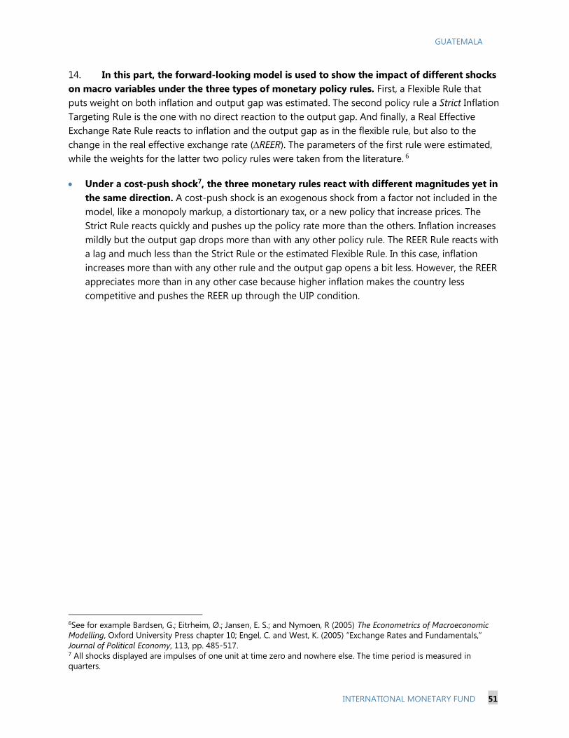
GUATEMALA
INTERNATIONAL MONETARY FUND 51
14. In this part, the forward-looking model is used to show the impact of different shocks
on macro variables under the three types of monetary policy rules. First, a Flexible Rule that
puts weight on both inflation and output gap was estimated. The second policy rule a Strict Inflation
Targeting Rule is the one with no direct reaction to the output gap. And finally, a Real Effective
Exchange Rate Rule reacts to inflation and the output gap as in the flexible rule, but also to the
change in the real effective exchange rate (REER). The parameters of the first rule were estimated,
while the weights for the latter two policy rules were taken from the literature. 6
Under a cost-push shock7, the three monetary rules react with different magnitudes yet in
the same direction. A cost-push shock is an exogenous shock from a factor not included in the
model, like a monopoly markup, a distortionary tax, or a new policy that increase prices. The
Strict Rule reacts quickly and pushes up the policy rate more than the others. Inflation increases
mildly but the output gap drops more than with any other policy rule. The REER Rule reacts with
a lag and much less than the Strict Rule or the estimated Flexible Rule. In this case, inflation
increases more than with any other rule and the output gap opens a bit less. However, the REER
appreciates more than in any other case because higher inflation makes the country less
competitive and pushes the REER up through the UIP condition.
6See for example Bardsen, G.; Eitrheim, Ø.; Jansen, E. S.; and Nymoen, R (2005) The Econometrics of Macroeconomic
Modelling, Oxford University Press chapter 10; Engel, C. and West, K. (2005) “Exchange Rates and Fundamentals,”
Journal of Political Economy, 113, pp. 485-517. 7 All shocks displayed are impulses of one unit at time zero and nowhere else. The time period is measured in
quarters.
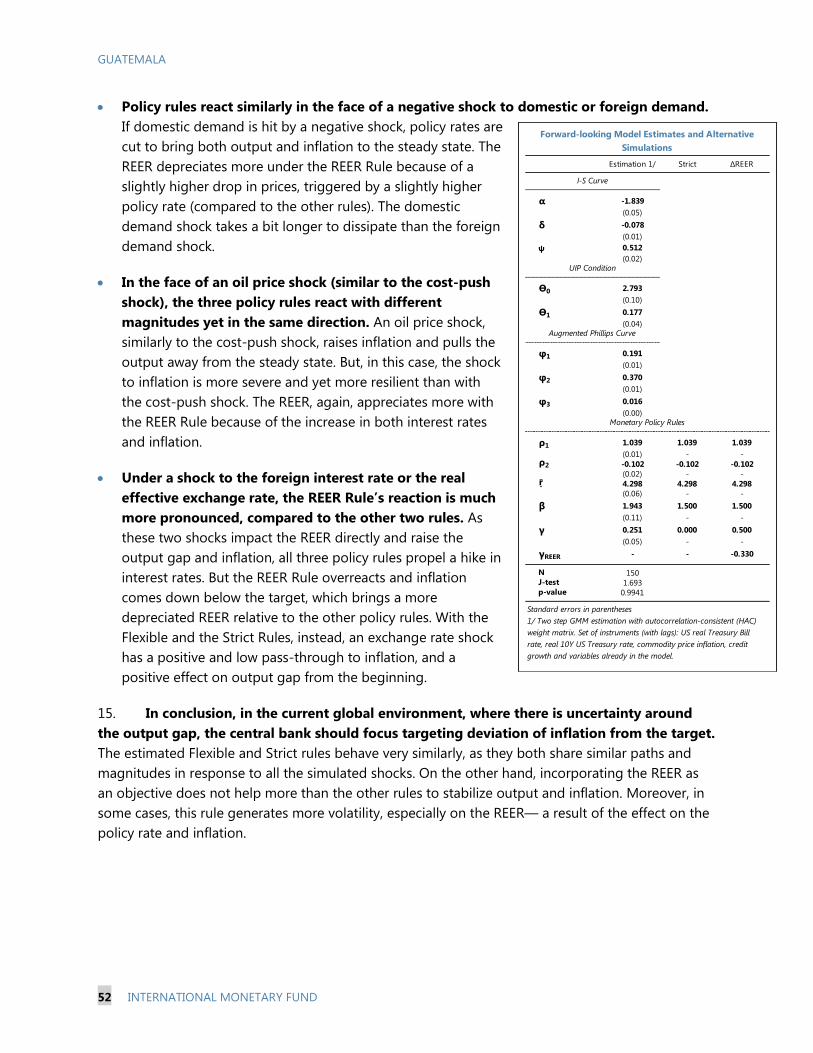
GUATEMALA
52 INTERNATIONAL MONETARY FUND
Policy rules react similarly in the face of a negative shock to domestic or foreign demand.
If domestic demand is hit by a negative shock, policy rates are
cut to bring both output and inflation to the steady state. The
REER depreciates more under the REER Rule because of a
slightly higher drop in prices, triggered by a slightly higher
policy rate (compared to the other rules). The domestic
demand shock takes a bit longer to dissipate than the foreign
demand shock.
In the face of an oil price shock (similar to the cost-push
shock), the three policy rules react with different
magnitudes yet in the same direction. An oil price shock,
similarly to the cost-push shock, raises inflation and pulls the
output away from the steady state. But, in this case, the shock
to inflation is more severe and yet more resilient than with
the cost-push shock. The REER, again, appreciates more with
the REER Rule because of the increase in both interest rates
and inflation.
Under a shock to the foreign interest rate or the real
effective exchange rate, the REER Rule’s reaction is much
more pronounced, compared to the other two rules. As
these two shocks impact the REER directly and raise the
output gap and inflation, all three policy rules propel a hike in
interest rates. But the REER Rule overreacts and inflation
comes down below the target, which brings a more
depreciated REER relative to the other policy rules. With the
Flexible and the Strict Rules, instead, an exchange rate shock
has a positive and low pass-through to inflation, and a
positive effect on output gap from the beginning.
15. In conclusion, in the current global environment, where there is uncertainty around
the output gap, the central bank should focus targeting deviation of inflation from the target.
The estimated Flexible and Strict rules behave very similarly, as they both share similar paths and
magnitudes in response to all the simulated shocks. On the other hand, incorporating the REER as
an objective does not help more than the other rules to stabilize output and inflation. Moreover, in
some cases, this rule generates more volatility, especially on the REER— a result of the effect on the
policy rate and inflation.
Estimation 1/ Strict ΔREER
α -1.839
(0.05)
δ -0.078
(0.01)
ψ 0.512
(0.02)
ϴ0 2.793
(0.10)
ϴ1 0.177
(0.04)
φ1 0.191
(0.01)
φ2 0.370
(0.01)
φ3 0.016
(0.00)
ρ1 1.039 1.039 1.039
(0.01) - -ρ2 -0.102 -0.102 -0.102
(0.02) - -ṝ 4.298 4.298 4.298
(0.06) - -
β 1.943 1.500 1.500
(0.11) - -
γ 0.251 0.000 0.500
(0.05) - -
γREER - - -0.330
N 150J-test 1.693p-value 0.9941
Standard errors in parentheses
Forward-looking Model Estimates and Alternative
Simulations
I-S Curve
UIP Condition
Augmented Phillips Curve
Monetary Policy Rules
1/ Two step GMM estimation with autocorrelation-consistent (HAC)
weight matrix. Set of instruments (with lags): US real Treasury Bill
rate, real 10Y US Treasury rate, commodity price inflation, credit
growth and variables already in the model.

GUATEMALA
INTERNATIONAL MONETARY FUND 53
Figure 1. Results: Cost-Push Shock (Positive)
Figure 2. Results: Domestic Demand Shock (Negative)
Figure 3. Results: Foreign Demand (Negative)

GUATEMALA
54 INTERNATIONAL MONETARY FUND
Figure 4. Results: Oil Price Shock (Positive)
Figure 5. Foreign Interest Rate Shock (Positive)
Figure 6. Exchange Rate Shock (Negative/Depreciation)

GUATEMALA
INTERNATIONAL MONETARY FUND 55
MACRO FINANCIAL LINKAGES: ASSESSING FINANCIAL
RISKS
A. Stress Testing the Financial System1
This section assesses the resilience of the banking system to a variety of shocks. We
employ financial soundness indicators and a top-down stress test to evaluate the health
of the banking system. The results suggest that the system could withstand a range of
sizable shocks but moderately high dollarization of bank loans, relatively large exposure
to the government, and growing bank foreign liabilities as well as maturity mismatches
in U.S. dollar positions represent vulnerabilities.
Introduction
1. Guatemala’s financial system is dominated by banks, which operate as part of financial
conglomerates. Financial system assets were 64 percent of GDP at end-2015, with banking system
assets representing 83 percent of the total. Most financial institutions (representing about 90
percent of total assets) are part of the 10 financial conglomerates operating in Guatemala, and the
majority of those that are part of conglomerates (2/3) are owned by the three largest domestic
conglomerates. Financial conglomerates are organized under a local bank and comprising domestic
and foreign subsidiaries as well as off-shore banks. Offshore banks represent about 8.4 percent of
total financial system assets, and their role is to raise deposits in U.S. dollars in Guatemala and lend
mainly to corporations in Guatemala and to a lesser extent to clients in other countries.2
2. The banking system has gone through consolidation and regionalization in recent
years. Concentration of assets has increased and five banks hold 80 percent of total banking system
assets. Latin American and U.S. banks hold 22 percent of
assets while Guatemalan banks hold subsidiaries in Costa,
Rica, El Salvador and Honduras, and lend abroad to
corporates and banks in these three countries.
3. The financial system appears sound though
capital is below the level of regional peers while
dollarization and external rollover risks continue to
represent vulnerabilities. At 14.1 percent,3 reported
regulatory capital is above the minimum requirement (10
1 Prepared by Iulia Ruxandra Teodoru. 2 Offshore banks need to be part of a financial group legally authorized in Guatemala and are subject to the same
supervision requirements as domestic banks. The main difference with domestic banks is that they cannot accept
small deposits (i.e. less than $10,000), deposits are not covered by the deposit insurance fund, and interest earnings
on deposits are not subject to taxes. Also, information submitted to SIB on deposits is aggregated without revealing
depositors’ or investors’ names. 3 The stress tests below are using a CAR of 13.9 percent (as of September 2015). The definition of CAR used in the
stress tests differs from the regulatory definition of capital.
0.0
5.0
10.0
15.0
20.0
25.0
Regulatory Capital to Risk-Weighted Assets (%)
Source: IMF FSIs.
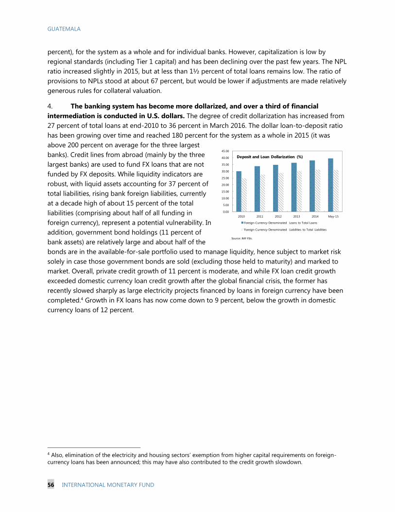
GUATEMALA
56 INTERNATIONAL MONETARY FUND
percent), for the system as a whole and for individual banks. However, capitalization is low by
regional standards (including Tier 1 capital) and has been declining over the past few years. The NPL
ratio increased slightly in 2015, but at less than 1½ percent of total loans remains low. The ratio of
provisions to NPLs stood at about 67 percent, but would be lower if adjustments are made relatively
generous rules for collateral valuation.
4. The banking system has become more dollarized, and over a third of financial
intermediation is conducted in U.S. dollars. The degree of credit dollarization has increased from
27 percent of total loans at end-2010 to 36 percent in March 2016. The dollar loan-to-deposit ratio
has been growing over time and reached 180 percent for the system as a whole in 2015 (it was
above 200 percent on average for the three largest
banks). Credit lines from abroad (mainly by the three
largest banks) are used to fund FX loans that are not
funded by FX deposits. While liquidity indicators are
robust, with liquid assets accounting for 37 percent of
total liabilities, rising bank foreign liabilities, currently
at a decade high of about 15 percent of the total
liabilities (comprising about half of all funding in
foreign currency), represent a potential vulnerability. In
addition, government bond holdings (11 percent of
bank assets) are relatively large and about half of the
bonds are in the available-for-sale portfolio used to manage liquidity, hence subject to market risk
solely in case those government bonds are sold (excluding those held to maturity) and marked to
market. Overall, private credit growth of 11 percent is moderate, and while FX loan credit growth
exceeded domestic currency loan credit growth after the global financial crisis, the former has
recently slowed sharply as large electricity projects financed by loans in foreign currency have been
completed.4 Growth in FX loans has now come down to 9 percent, below the growth in domestic
currency loans of 12 percent.
4 Also, elimination of the electricity and housing sectors’ exemption from higher capital requirements on foreign-
currency loans has been announced; this may have also contributed to the credit growth slowdown.
0.00
5.00
10.00
15.00
20.00
25.00
30.00
35.00
40.00
45.00
2010 2011 2012 2013 2014 May-15
Foreign-Currency-Denominated Loans to Total Loans
Foreign-Currency-Denominated Liabilities to Total Liabilities
Deposit and Loan Dollarization (%)
Source: IMF FSIs.
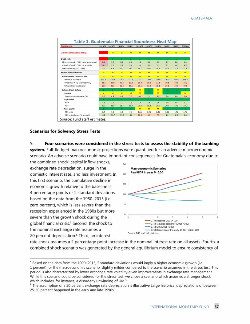
GUATEMALA
INTERNATIONAL MONETARY FUND 57
Table 1. Guatemala: Financial Soundness Heat Map
Source: Fund staff estimates.
Scenarios for Solvency Stress Tests
5. Four scenarios were considered in the stress tests to assess the stability of the banking
system. Full-fledged macroeconomic projections were quantified for an adverse macroeconomic
scenario. An adverse scenario could have important consequences for Guatemala's economy due to
the combined shock: capital inflow shocks,
exchange rate depreciation, surge in the
domestic interest rate, and less investment. In
this first scenario, the cumulative decline in
economic growth relative to the baseline is
4 percentage points or 2 standard deviations
based on the data from the 1980–2015 (i.e.
zero percent), which is less severe than the
recession experienced in the 1980s but more
severe than the growth shock during the
global financial crisis.5 Second, the shock to
the nominal exchange rate assumes a
20 percent depreciation.6 Third, an interest
rate shock assumes a 2 percentage point increase in the nominal interest rate on all assets. Fourth, a
combined shock scenario was generated by the general equilibrium model to ensure consistency of
5 Based on the data from the 1990–2015, 2 standard deviations would imply a higher economic growth (i.e.
1 percent) for the macroeconomic scenario, slightly milder compared to the scenario assumed in the stress test. This
period is also characterized by lower exchange rate volatility given improvements in exchange rate management.
While this scenario could be considered for the stress test, we chose a scenario which assumes a stronger shock
which includes, for instance, a disorderly unwinding of UMP. 6 The assumption of a 20 percent exchange rate depreciation is illustrative Large historical depreciations of between
25-50 percent happened in the early and late 1990s.
Guatemala 2013Q2 2013Q3 2013Q4 2014Q1 2014Q2 2014Q3 2014Q4 2015Q1 2015Q2 2015Q3
Overall Financial Sector Rating H M M M M M M M M M
Credit cycle H L L L L L L L L L
Change in credit / GDP ratio (pp, annual) 6.3 1.7 0.9 0.9 1.0 0.2 0.3 0.7 1.0 1.6
Growth of credit / GDP (%, annual) 25.2 5.7 2.9 2.9 3.3 0.6 1.1 2.3 3.0 4.9
Credit-to-GDP gap (st. dev) 1.0 0.6 0.0 -0.8 -1.2 -1.6 -1.5 -1.6 -1.4 -1.2
Balance Sheet Soundness M M M M M M M M M M
Balance Sheet Structural Risk M M M M M M M M M M
Deposit-to-loan ratio 134.2 129.1 129.9 131.9 131.2 129.8 128.9 129.4 129.6 125.6
FX liabilities % (of total liabilities) 28.2 29.0 30.3 30.4 30.4 30.9 31.1 30.8 30.8 31.1
FX loans % (of total loans) 35.2 36.6 36.3 36.1 37.1 37.2 38.1 39.0 39.4 39.9
Balance Sheet Buffers L L L L M L M L L L
Leverage M M M M M L M L L M
Capital-to-assets ratio (%) 7.0 6.8 6.9 7.0 6.9 7.1 6.9 7.0 7.0 7.0
Profitability L L L L L L L L L L
ROA 1.9 2.0 2.0 1.9 1.9 1.8 1.9 1.9 1.8 1.7
ROE 20.5 21.5 21.4 21.0 20.4 19.3 20.6 20.7 19.9 19.2
Asset quality L L L L M M M L L L
NPL ratio 1.4 1.3 1.2 1.3 1.56 1.41 1.29 1.35 1.45 1.43
NPL ratio change (%, annual) -8.0 -13.7 -11.3 -3.0 13.3 6.1 7.9 3.6 -6.9 1.8
80
90
100
110
120
130
0 1 2 3 4 5 6
GTM Baseline (2015=100)
GTM "adverse scenario" (2015=100)
GTM GFC (2008=100)
GTM Recession of the early 1980s (1981=100)
Macroeconomic Scenarios
Real GDP in year 0=100
Source: IMF staff calculations.
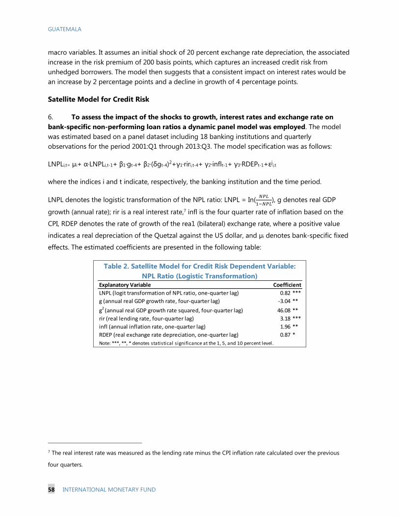
GUATEMALA
58 INTERNATIONAL MONETARY FUND
macro variables. It assumes an initial shock of 20 percent exchange rate depreciation, the associated
increase in the risk premium of 200 basis points, which captures an increased credit risk from
unhedged borrowers. The model then suggests that a consistent impact on interest rates would be
an increase by 2 percentage points and a decline in growth of 4 percentage points.
Satellite Model for Credit Risk
6. To assess the impact of the shocks to growth, interest rates and exchange rate on
bank-specific non-performing loan ratios a dynamic panel model was employed. The model
was estimated based on a panel dataset including 18 banking institutions and quarterly
observations for the period 2001:Q1 through 2013:Q3. The model specification was as follows:
LNPLi,t= µi+ α·LNPLi,t-1+ β1·gt-4+ β2·(δgt-4)2+γ1·riri,t-4+ γ2·inflt-1+ γ3·RDEPt-1+εji,t
where the indices i and t indicate, respectively, the banking institution and the time period.
LNPL denotes the logistic transformation of the NPL ratio: LNPL = In(𝑁𝑃𝐿
1−𝑁𝑃𝐿), g denotes real GDP
growth (annual rate); rir is a real interest rate,7 infl is the four quarter rate of inflation based on the
CPI, RDEP denotes the rate of growth of the rea1 (bilateral) exchange rate, where a positive value
indicates a real depreciation of the Quetzal against the US dollar, and µi denotes bank-specific fixed
effects. The estimated coefficients are presented in the following table:
Table 2. Satellite Model for Credit Risk Dependent Variable:
NPL Ratio (Logistic Transformation)
7 The real interest rate was measured as the lending rate minus the CPI inflation rate calculated over the previous
four quarters.
Explanatory Variable
LNPL (logit transformation of NPL ratio, one-quarter lag) 0.82 ***
g (annual real GDP growth rate, four-quarter lag) -3.04 **
g2 (annual real GDP growth rate squared, four-quarter lag) 46.08 **
rir (real lending rate, four-quarter lag) 3.18 ***
infl (annual inflation rate, one-quarter lag) 1.96 **
RDEP (real exchange rate depreciation, one-quarter lag) 0.87 *
Note: ***, **, * denotes statistical significance at the 1, 5, and 10 percent level.
Coefficient

GUATEMALA
INTERNATIONAL MONETARY FUND 59
The estimated model is non-linear in real GDP growth: the NPL ratio increases at an accelerated rate
as real GDP growth declines further. Similar results were obtained using slightly different
specifications of the equation above.
Overall, the NPL-ratio under stress was computed as:
𝑁𝑃𝐿𝑡𝑠𝑡𝑟𝑒𝑠𝑠 = (
𝑁𝑃𝐿𝑡−1𝑖𝑛𝑖𝑡𝑖𝑎𝑙
1 − 𝑁𝑃𝐿𝑡−1𝑖𝑛𝑖𝑡𝑖𝑎𝑙) 𝑒𝑥𝑝{𝛽∆𝑋𝑡} /[1 + (
𝑁𝑃𝐿𝑡−1𝑖𝑛𝑖𝑡𝑖𝑎𝑙
1 − 𝑁𝑃𝐿𝑡−1𝑖𝑛𝑖𝑡𝑖𝑎𝑙) 𝑒𝑥𝑝{𝛽∆𝑋𝑡}]
where 𝑋𝑡 is the vector of macroeconomic factors used and β is the vector of coefficients (from the
credit risk model). ∆𝑋𝑡 represents the change in the levels of macro variables.
7. An adjustment of provisions and initial capital was also made. Specifically, effective
provisioning rates were calculated as follows:
Adjusted effective provisioning rate=Nominal provisioning rate*(1−Adjusted collateral value
Loan value)
The tests are undertaken under more rigorous rules for collateral valuation, given the difficulty
encountered by the banks in recovering collateral. Collateral values are discounted 20 percent
relative to the current market values, and a further adjustment is introduced to take account of the
average time to recover collateral via lawsuits—about 3 years. Thus, the adjusted collateral value is
calculated as follows:
Adjusted collateral value=Original collateral value*0.8*(1+0.07)-3
In the calculation, the discount rate is set at 7 percent. This value approximates the nominal interest
rate at a 3year horizon corresponding to the baseline yield curve in domestic currency.
With respect to the capital used in the stress tests for the capital adequacy ratio, the capital
considered is the equity of banks and does not include such instruments as subordinated debt and
other hybrid capital, while the regulatory capital typically counts these instruments as capital.
8. Estimates from the credit risk model suggest that credit risk in the loan book is an
important risk factor for the banking system. Loans to the economy represent more than half of
total banking sector assets, of which a large share is directed towards the corporate sector. As a
result of the decline in GDP growth, the depreciation of the Quetzal, and the rise in interest rates,
the NPL ratios increase by 1 percentage point in the adverse scenario.
Results of Solvency Stress Tests
9. Banks appear quite resilient to high levels of stress, but there are areas of
vulnerability.

GUATEMALA
60 INTERNATIONAL MONETARY FUND
After making adjustments to provisions to conduct the tests under more rigorous rules for
collateral valuation and calculation of loan loss provisions, initial capital was adjusted
downwards by 0.6 percentage points.
Under the adverse growth scenario (i.e. zero percent
economic growth, see sections on “Scenarios for
Solvency Stress Tests” and “Satellite Model for Credit
Risk”), the CAR for the system falls by 0.9 percentage
points.
Direct exchange rate risk is contained, given that most
banks hold positive net open FX positions in foreign
currency, with assets more than offsetting liabilities
denominated in U.S. dollars. The net open position is
equivalent to 1.3 percent of total assets, and it is negative
in only three banks (equivalent to less than 1 percent of
assets in 2 banks and 1.6 percent of the assets of a third bank). The situation implies that the
banks would benefit from a depreciation of the Quetzal if the “indirect” credit risks associated
with the depreciation are ignored. The CAR for the system would improve by 0.4 percentage
points, with a depreciation of 20 percent vis-a-vis the U.S. dollar.
Indirect exchange rate risk, however, could trigger credit losses. A depreciation of the Quetzal by
20 percent would increase the debt burden and reduce the repayment capacity of un-hedged
foreign currency borrowers. Based on the estimated model for credit risk (see section on
“Satellite Model for Credit Risk”), having a 20 percent depreciation will make 13 percent of FX
loans become NPLs, which would cause a 0.9 percentage points decline in the CAR. In a different
and more adverse scenario, the assumption is that 40 percent of FX loans become NPLs, given
that 40 percent of borrowers in foreign currency are un-hedged. This causes a 2.5 percentage
points decline in the CAR. In this latter scenario, if the effects from both direct and indirect
exchange rate risks are combined, the CAR falls by 2.1 percentage points.
Potential losses, in particular for larger banks, driven by interest rate risk, which materializes
because of losses in interest income and valuation losses on government bonds, are notable.
The valuation losses correspond to bonds held in the “available for sale” portfolios that were
marked to market. As a result of securities losses, the CAR declines by 2.6 percentage points. If
both the net interest income and repricing impacts are assessed, the CAR falls by 2.8 percentage
points.
While the banking system can handle individual shocks well, a combined shock scenario based
on a consistent set of assumptions from a general equilibrium macro model with the initial
shock of 20 percent depreciation and an increase in interest rates of 2 percentage points would
lead to an increase in credit risk from un-hedged borrowers and to valuation losses on
government bonds, and will push the capital ratio below the regulatory minimum (i.e. the CAR
falls by 7 percentage points).
0
2
4
6
8
10
12
14
16
Credit Risk FX Risk Interest Rate Risk Combined Risk
(Credit, FX, and
Interest Rate Risk)
Pre-Shock Post-Shock Minimum Threshold
Source: IMF staff calculations.
Note: Solvency stress test for FX risk assumes 20percent depreciation; test for interest rate risk assumes a 2 percentage points nominal interest rate increase; test for combined risk adds impact on the CAR from credit, FX, and interest rate risks.
Impact of Stress on the CAR(Percent)

GUATEMALA
INTERNATIONAL MONETARY FUND 61
Results of Liquidity Stress Tests
10. Banks appear quite resilient to severe liquidity shocks, but there are areas of
weakness.
Liquidity stress tests assumed a combination of 10 percent run-off rates on domestic currency
and FX deposits, and 5 percent on other FX liabilities and 3
percent on other domestic currency liabilities per month.
Under this scenario most banks would remain liquid after 5
months. If 15 percent run-off rates per month are assumed
on domestic currency and FX deposits (and the same run-
off rates as above on other domestic currency and FX
liabilities), more than half of the system becomes illiquid
after 5 months.
Alternatively, if the impact from a 25 percent run-off rates
on FX deposits, and 35 percent run-off rates on other FX
liabilities (e.g. foreign credit lines) is assessed, one large
and one middle-sized bank become illiquid after 5 months.
Thus, reliance on foreign credit lines represents an area of vulnerability.
Maturity mismatches in U.S. dollar positions (which are presumably higher than in domestic
currency positions, in particular in the short term) could represent a significant vulnerability
though this could not be tested due to the lack of data on the maturity structure of assets and
liabilities.
0
10
20
30
40
50
60
Liquid Assets to Total Assets Liquid Assets to Short-Term Liabilities
Pre-Shock Post-Shock
Impact of Stress on Liquid Assets(Percent)
Source: IMF staff calculations.Note: Liquidity stress test assumes a 10 and 5 percent per month withdrawal of domestic demand deposits and other liabilities respectively, and a 10 and 3 percent per month withdrawal offoreign demand deposits and other foreign liabilities respectively.

GUATEMALA
62 INTERNATIONAL MONETARY FUND
Table 3. Banking Sector Financial Soundness Indicators
Selected Banking Sector Ratios All Banks
Capital Adequacy
Total capital / RWA (CAR) 13.9
Asset Quality
NPLs (gross)/ total loans 1.5
Specific Provisions/NPLs 66.9
(NPLs-specific provisions)/capital 3.0
FX loans/total loans 40.4
RWA/total assets 66.2
Profitability
ROA (after-tax) 1.2
ROE (after-tax) 13.4
Liquidity
Liquid assets/total assets 37.8
Liquid assets/short-term liabilities 52.0
Sensitivity to Market Risk
Net FX exposure / capital 14.2
Basic Ratio Analysis: Ratings 1/
Overall 1.8
Capital Adequacy
Total capital / RWA (CAR) 1.7
Asset Quality
NPLs (gross)/ total loans 1.0
Provisions/NPLs 2.4
(NPLs-provisions)/capital 1.0
FX loans/total loans 2.6
RWA/total assets 3.0
Profitability
ROA (after-tax) 2.3
ROE (after-tax) 2.1
Liquidity
Liquid assets/total assets 1.1
Liquid assets/short-term liabilities 1.7
Sensitivity to Market Risk
Net FX exposure / capital 2.5
The ratings are averaged across banks.
1/ 1=low risk, 2=increased risk, 3=high risk, 4=very high risk.
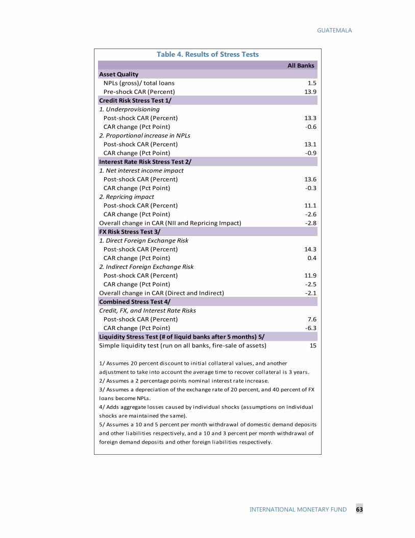
GUATEMALA
INTERNATIONAL MONETARY FUND 63
Table 4. Results of Stress Tests
All Banks
Asset Quality
NPLs (gross)/ total loans 1.5
Pre-shock CAR (Percent) 13.9
Credit Risk Stress Test 1/
1. Underprovisioning
Post-shock CAR (Percent) 13.3
CAR change (Pct Point) -0.6
2. Proportional increase in NPLs
Post-shock CAR (Percent) 13.1
CAR change (Pct Point) -0.9
Interest Rate Risk Stress Test 2/
1. Net interest income impact
Post-shock CAR (Percent) 13.6
CAR change (Pct Point) -0.3
2. Repricing impact
Post-shock CAR (Percent) 11.1
CAR change (Pct Point) -2.6
Overall change in CAR (NII and Repricing Impact) -2.8
FX Risk Stress Test 3/
1. Direct Foreign Exchange Risk
Post-shock CAR (Percent) 14.3
CAR change (Pct Point) 0.4
2. Indirect Foreign Exchange Risk
Post-shock CAR (Percent) 11.9
CAR change (Pct Point) -2.5
Overall change in CAR (Direct and Indirect) -2.1
Combined Stress Test 4/
Credit, FX, and Interest Rate Risks
Post-shock CAR (Percent) 7.6
CAR change (Pct Point) -6.3
Liquidity Stress Test (# of liquid banks after 5 months) 5/
Simple liquidity test (run on all banks, fire-sale of assets) 15
1/ Assumes 20 percent discount to initial collateral values, and another
adjustment to take into account the average time to recover collateral is 3 years.
2/ Assumes a 2 percentage points nominal interest rate increase.
3/ Assumes a depreciation of the exchange rate of 20 percent, and 40 percent of FX
loans become NPLs.
4/ Adds aggregate losses caused by individual shocks (assumptions on individual
shocks are maintained the same).
5/ Assumes a 10 and 5 percent per month withdrawal of domestic demand deposits
and other l iabilities respectively, and a 10 and 3 percent per month withdrawal of
foreign demand deposits and other foreign liabilities respectively.
Results of Stress Tests

GUATEMALA
64 INTERNATIONAL MONETARY FUND
B. Domestic Bank Network Analysis and Cross-Border Financial Spillovers8
The recent financial crisis has proven that stress events in individual institutions can spill
over and undermine the stability of the entire financial system, highlighting the need to
track direct and indirect financial interconnections among financial institutions. This note
looks at domestic interbank linkages and cross-border bank interconnections in
Guatemala to assess whether linkages across institutions within and beyond the country’s
borders may have systematic implications. Results suggest that the Guatemalan banking
sector is relatively resilient to shocks originating both domestically and abroad though
some banks deserve higher scrutiny in terms of their vulnerability and the level of
contagion they can generate.
Bank Network Analysis
11. To assess potential systemic implications of domestic interbank linkages we simulate
the cascading effect upon the failure of selected banks due to credit and funding shocks. We
do so by using the interbank exposure model developed by Espinosa and Sole (2010)9 which is
designed to track the domino effects triggered by the hypothetical default of each bank in the
system through the resulting credit losses and funding shortfalls (Figure 1).
12. The analysis is based on a stylized balance sheet identity that highlights the role of
interbank exposures. In the identity, bank loans and other assets are funded by (i) capital, (ii) long-
and short-term borrowing excluding interbank loans, (iii) deposits, and (iv) interbank borrowing. To
analyze the effect of a credit shock, the model simulates the individual default of each institution’s
interbank obligations in the network. For different assumptions of loss given default, it is assumed
that the capital of creditor banks absorbs the losses on impact, triggering the creditor bank’s default
if its capital is insufficient to fully cover losses. In addition to its direct credit exposures to other
institutions, a bank’s vulnerability also stems from its inability to roll over all or part of its funding in
the interbank market, and thus having to sell assets at a discount in order to re-establish its balance
sheet identity. In this respect, a credit shock may be compounded by a funding shock and associated
fire sales losses if default of an institution also leads to a liquidity squeeze. In the model, it is assumed
that institutions are unable to replace all the funding previously granted by the defaulted institutions,
which in turns generates a fire sale of assets. Default is again triggered if bank capital is not enough
to absorb the funding-shortfall induced loss.10
8 Prepared by Valentina Flamini. 9 Espinosa-Vega, M. and J. Sole, 2012, “Cross-Border Financial Surveillance: A Network Perspective,” IMF WP/10/105,
Washington, DC. 10 Calculations assume 100 percent loss given default and funding shortfall, and 10 percent of lost funding being
non-replaceable. Interbank exposure and capital data are as of December 31, 2015.
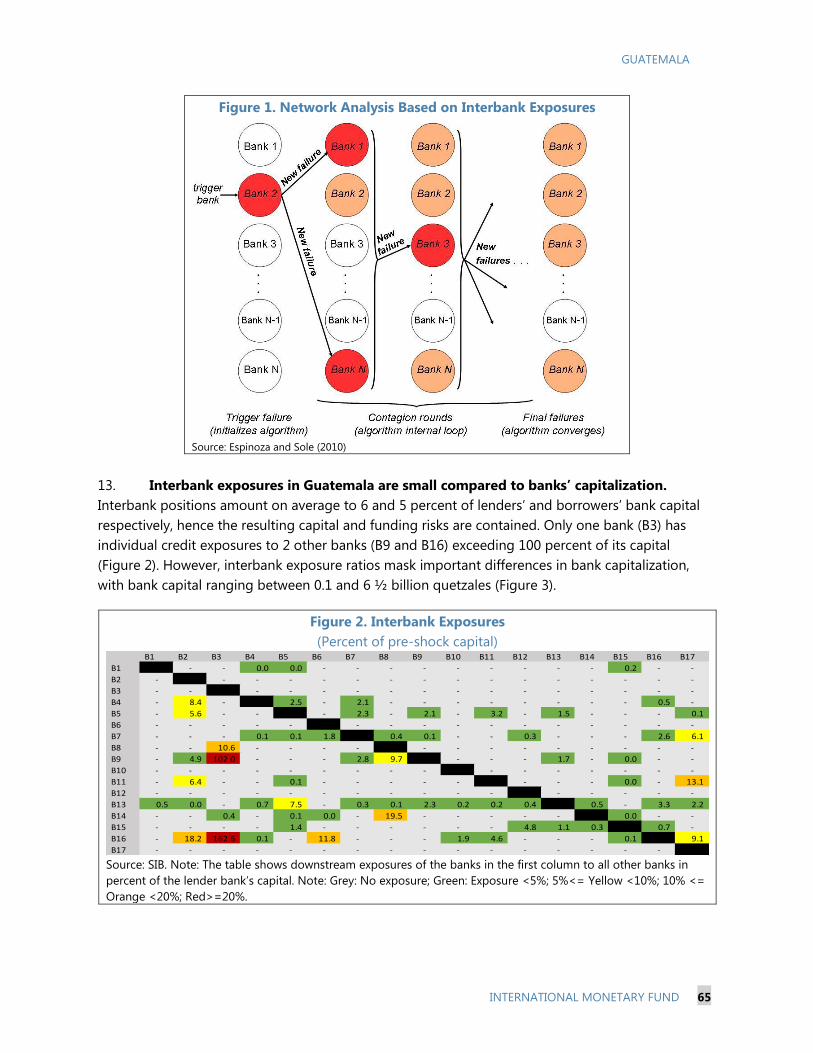
GUATEMALA
INTERNATIONAL MONETARY FUND 65
Figure 1. Network Analysis Based on Interbank Exposures
Source: Espinoza and Sole (2010)
13. Interbank exposures in Guatemala are small compared to banks’ capitalization.
Interbank positions amount on average to 6 and 5 percent of lenders’ and borrowers’ bank capital
respectively, hence the resulting capital and funding risks are contained. Only one bank (B3) has
individual credit exposures to 2 other banks (B9 and B16) exceeding 100 percent of its capital
(Figure 2). However, interbank exposure ratios mask important differences in bank capitalization,
with bank capital ranging between 0.1 and 6 ½ billion quetzales (Figure 3).
Figure 2. Interbank Exposures
(Percent of pre-shock capital)
Source: SIB. Note: The table shows downstream exposures of the banks in the first column to all other banks in
percent of the lender bank’s capital. Note: Grey: No exposure; Green: Exposure <5%; 5%<= Yellow <10%; 10% <=
Orange <20%; Red>=20%.
B1 B2 B3 B4 B5 B6 B7 B8 B9 B10 B11 B12 B13 B14 B15 B16 B17
B1 - - - 0.0 0.0 - - - - - - - - - 0.2 - -
B2 - - - - - - - - - - - - - - - - -
B3 - - - - - - - - - - - - - - - - -
B4 - 8.4 - - 2.5 - 2.1 - - - - - - - - 0.5 -
B5 - 5.6 - - - - 2.3 - 2.1 - 3.2 - 1.5 - - - 0.1
B6 - - - - - - - - - - - - - - - - -
B7 - - - 0.1 0.1 1.8 - 0.4 0.1 - - 0.3 - - - 2.6 6.1
B8 - - 10.6 - - - - - - - - - - - - - -
B9 - 4.9 102.0 - - - 2.8 9.7 - - - - 1.7 - 0.0 - -
B10 - - - - - - - - - - - - - - - - -
B11 - 6.4 - - 0.1 - - - - - - - - - 0.0 - 13.1
B12 - - - - - - - - - - - - - - - - -
B13 0.5 0.0 - 0.7 7.5 - 0.3 0.1 2.3 0.2 0.2 0.4 - 0.5 - 3.3 2.2
B14 - - 0.4 - 0.1 0.0 - 19.5 - - - - - - 0.0 - -
B15 - - - - 1.4 - - - - - - 4.8 1.1 0.3 - 0.7 -
B16 - 18.2 162.6 0.1 - 11.8 - - - 1.9 4.6 - - - 0.1 - 9.1
B17 - - - - - - - - - - - - - - - - -
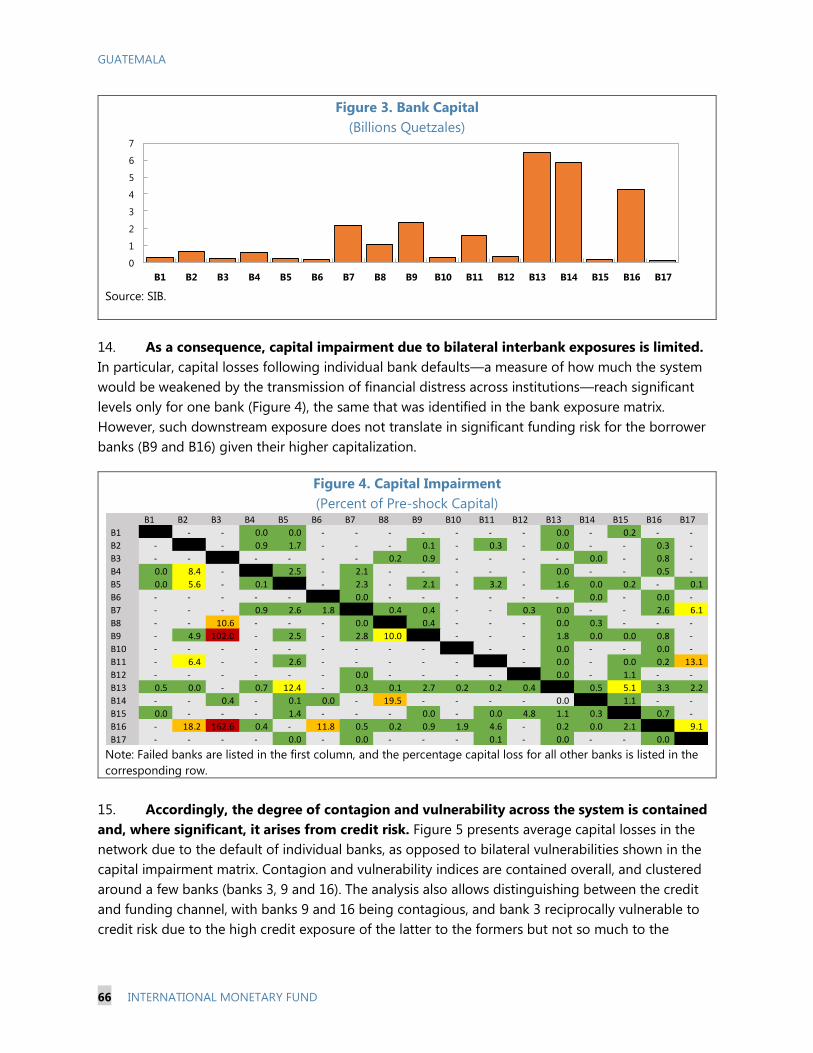
GUATEMALA
66 INTERNATIONAL MONETARY FUND
Figure 3. Bank Capital
(Billions Quetzales)
Source: SIB.
14. As a consequence, capital impairment due to bilateral interbank exposures is limited.
In particular, capital losses following individual bank defaults—a measure of how much the system
would be weakened by the transmission of financial distress across institutions—reach significant
levels only for one bank (Figure 4), the same that was identified in the bank exposure matrix.
However, such downstream exposure does not translate in significant funding risk for the borrower
banks (B9 and B16) given their higher capitalization.
Figure 4. Capital Impairment
(Percent of Pre-shock Capital)
Note: Failed banks are listed in the first column, and the percentage capital loss for all other banks is listed in the
corresponding row.
15. Accordingly, the degree of contagion and vulnerability across the system is contained
and, where significant, it arises from credit risk. Figure 5 presents average capital losses in the
network due to the default of individual banks, as opposed to bilateral vulnerabilities shown in the
capital impairment matrix. Contagion and vulnerability indices are contained overall, and clustered
around a few banks (banks 3, 9 and 16). The analysis also allows distinguishing between the credit
and funding channel, with banks 9 and 16 being contagious, and bank 3 reciprocally vulnerable to
credit risk due to the high credit exposure of the latter to the formers but not so much to the
0
1
2
3
4
5
6
7
B1 B2 B3 B4 B5 B6 B7 B8 B9 B10 B11 B12 B13 B14 B15 B16 B17
B1 B2 B3 B4 B5 B6 B7 B8 B9 B10 B11 B12 B13 B14 B15 B16 B17
B1 -- - - 0.0 0.0 - - - - - - - 0.0 - 0.2 - -
B2 - -- - 0.9 1.7 - - - 0.1 - 0.3 - 0.0 - - 0.3 -
B3 - - -- - - - - 0.2 0.9 - - - - 0.0 - 0.8 -
B4 0.0 8.4 - -- 2.5 - 2.1 - - - - - 0.0 - - 0.5 -
B5 0.0 5.6 - 0.1 -- - 2.3 - 2.1 - 3.2 - 1.6 0.0 0.2 - 0.1
B6 - - - - - -- 0.0 - - - - - - 0.0 - 0.0 -
B7 - - - 0.9 2.6 1.8 -- 0.4 0.4 - - 0.3 0.0 - - 2.6 6.1
B8 - - 10.6 - - - 0.0 -- 0.4 - - - 0.0 0.3 - - -
B9 - 4.9 102.0 - 2.5 - 2.8 10.0 -- - - - 1.8 0.0 0.0 0.8 -
B10 - - - - - - - - - -- - - 0.0 - - 0.0 -
B11 - 6.4 - - 2.6 - - - - - -- - 0.0 - 0.0 0.2 13.1
B12 - - - - - - 0.0 - - - - -- 0.0 - 1.1 - -
B13 0.5 0.0 - 0.7 12.4 - 0.3 0.1 2.7 0.2 0.2 0.4 -- 0.5 5.1 3.3 2.2
B14 - - 0.4 - 0.1 0.0 - 19.5 - - - - 0.0 -- 1.1 - -
B15 0.0 - - - 1.4 - - - 0.0 - 0.0 4.8 1.1 0.3 -- 0.7 -
B16 - 18.2 162.6 0.4 - 11.8 0.5 0.2 0.9 1.9 4.6 - 0.2 0.0 2.1 -- 9.1
B17 - - - - 0.0 - 0.0 - - - 0.1 - 0.0 - - 0.0 --
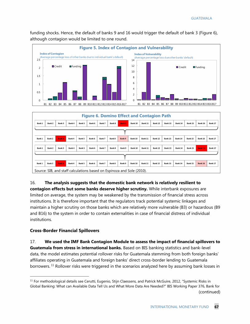
GUATEMALA
INTERNATIONAL MONETARY FUND 67
funding shocks. Hence, the default of banks 9 and 16 would trigger the default of bank 3 (Figure 6),
although contagion would be limited to one round.
Figure 5. Index of Contagion and Vulnerability
Figure 6. Domino Effect and Contagion Path
Source: SIB, and staff calculations based on Espinoza and Sole (2010).
16. The analysis suggests that the domestic bank network is relatively resilient to
contagion effects but some banks deserve higher scrutiny. While interbank exposures are
limited on average, the system may be weakened by the transmission of financial stress across
institutions. It is therefore important that the regulators track potential systemic linkages and
maintain a higher scrutiny on those banks which are relatively more vulnerable (B3) or hazardous (B9
and B16) to the system in order to contain externalities in case of financial distress of individual
institutions.
Cross-Border Financial Spillovers
17. We used the IMF Bank Contagion Module to assess the impact of financial spillovers to
Guatemala from stress in international banks. Based on BIS banking statistics and bank-level
data, the model estimates potential rollover risks for Guatemala stemming from both foreign banks’
affiliates operating in Guatemala and foreign banks’ direct cross-border lending to Guatemala
borrowers. 11 Rollover risks were triggered in the scenarios analyzed here by assuming bank losses in
11 For methodological details see Cerutti, Eugenio, Stijn Claessens, and Patrick McGuire, 2012, “Systemic Risks in
Global Banking: What can Available Data Tell Us and What More Data Are Needed?” BIS Working Paper 376, Bank for
(continued)
0
0.5
1
1.5
2
2.5
B1 B2 B3 B4 B5 B6 B7 B8 B9 B10 B11 B12 B13 B14 B15 B16 B17
Credit Funding
Index of Contagion
(Average percentage loss of other banks due to individual bank's default)
0
2
4
6
8
10
12
14
B1 B2 B3 B4 B5 B6 B7 B8 B9 B10 B11 B12 B13 B14 B15 B16 B17
Credit Funding
Index of Vulnerability
(Average percentage loss due other banks' default)
Bank 1 Bank 2 Bank 3 Bank 4 Bank 5 Bank 7Bank 6 Bank 8 Bank 15Bank 9 Bank 13Bank 10 Bank 11 Bank 14Bank 12 Bank 16
Bank 1 Bank 2 Bank 3 Bank 4 Bank 5 Bank 7Bank 6 Bank 8 Bank 15Bank 9 Bank 13Bank 10 Bank 11 Bank 14Bank 12 Bank 16
Bank 17
Bank 17
Bank 1 Bank 2 Bank 3 Bank 4 Bank 5 Bank 7Bank 6 Bank 8 Bank 15Bank 9 Bank 13Bank 10 Bank 11 Bank 14Bank 12 Bank 16
Bank 1 Bank 2 Bank 3 Bank 4 Bank 5 Bank 7Bank 6 Bank 8 Bank 15Bank 9 Bank 13Bank 10 Bank 11 Bank 14Bank 12 Bank 16
Bank 17
Bank 17
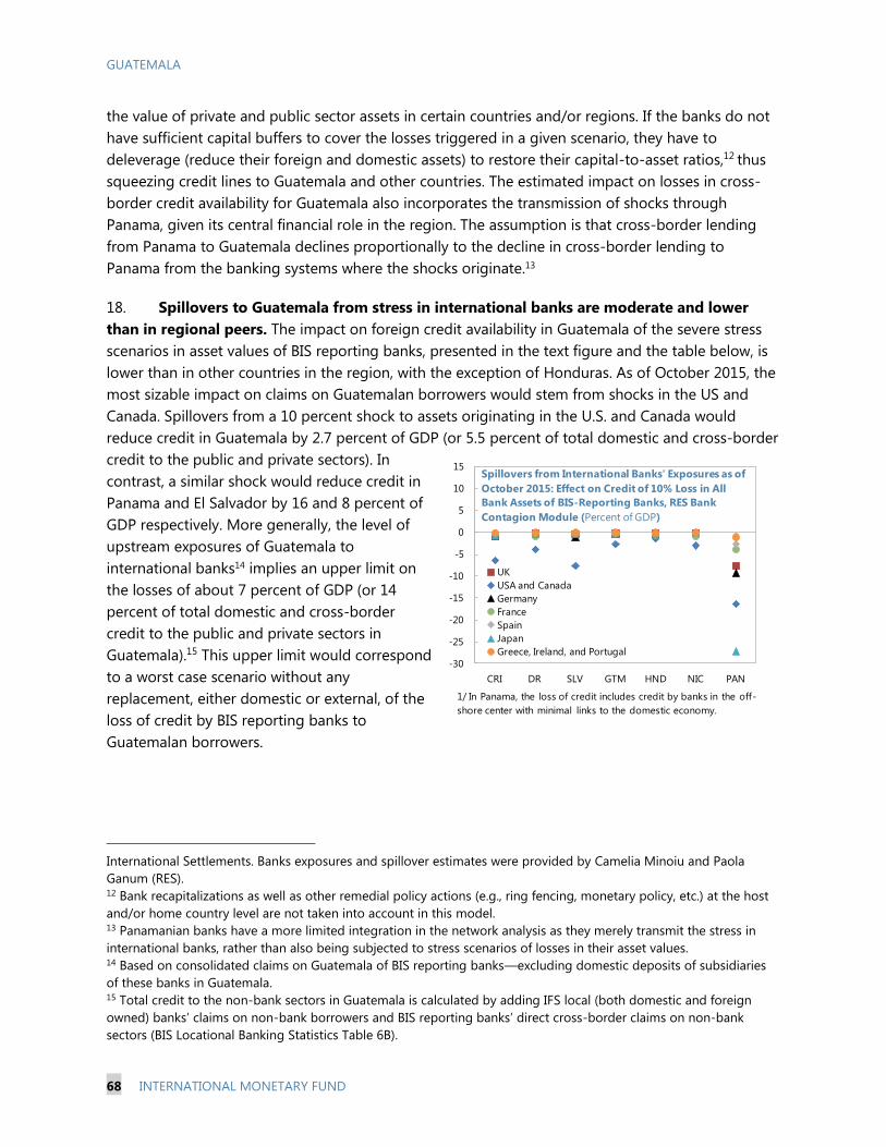
GUATEMALA
68 INTERNATIONAL MONETARY FUND
the value of private and public sector assets in certain countries and/or regions. If the banks do not
have sufficient capital buffers to cover the losses triggered in a given scenario, they have to
deleverage (reduce their foreign and domestic assets) to restore their capital-to-asset ratios,12 thus
squeezing credit lines to Guatemala and other countries. The estimated impact on losses in cross-
border credit availability for Guatemala also incorporates the transmission of shocks through
Panama, given its central financial role in the region. The assumption is that cross-border lending
from Panama to Guatemala declines proportionally to the decline in cross-border lending to
Panama from the banking systems where the shocks originate.13
18. Spillovers to Guatemala from stress in international banks are moderate and lower
than in regional peers. The impact on foreign credit availability in Guatemala of the severe stress
scenarios in asset values of BIS reporting banks, presented in the text figure and the table below, is
lower than in other countries in the region, with the exception of Honduras. As of October 2015, the
most sizable impact on claims on Guatemalan borrowers would stem from shocks in the US and
Canada. Spillovers from a 10 percent shock to assets originating in the U.S. and Canada would
reduce credit in Guatemala by 2.7 percent of GDP (or 5.5 percent of total domestic and cross-border
credit to the public and private sectors). In
contrast, a similar shock would reduce credit in
Panama and El Salvador by 16 and 8 percent of
GDP respectively. More generally, the level of
upstream exposures of Guatemala to
international banks14 implies an upper limit on
the losses of about 7 percent of GDP (or 14
percent of total domestic and cross-border
credit to the public and private sectors in
Guatemala).15 This upper limit would correspond
to a worst case scenario without any
replacement, either domestic or external, of the
loss of credit by BIS reporting banks to
Guatemalan borrowers.
International Settlements. Banks exposures and spillover estimates were provided by Camelia Minoiu and Paola
Ganum (RES). 12 Bank recapitalizations as well as other remedial policy actions (e.g., ring fencing, monetary policy, etc.) at the host
and/or home country level are not taken into account in this model. 13 Panamanian banks have a more limited integration in the network analysis as they merely transmit the stress in
international banks, rather than also being subjected to stress scenarios of losses in their asset values. 14 Based on consolidated claims on Guatemala of BIS reporting banks—excluding domestic deposits of subsidiaries
of these banks in Guatemala. 15 Total credit to the non-bank sectors in Guatemala is calculated by adding IFS local (both domestic and foreign
owned) banks’ claims on non-bank borrowers and BIS reporting banks’ direct cross-border claims on non-bank
sectors (BIS Locational Banking Statistics Table 6B).
-30
-25
-20
-15
-10
-5
0
5
10
15
CRI DR SLV GTM HND NIC PAN
UK
USA and Canada
Germany
France
Spain
Japan
Greece, Ireland, and Portugal
Spillovers from International Banks' Exposures as of
October 2015: Effect on Credit of 10% Loss in All
Bank Assets of BIS-Reporting Banks, RES Bank
Contagion Module (Percent of GDP)
1/ In Panama, the loss of credit includes credit by banks in the off-
shore center with minimal links to the domestic economy.
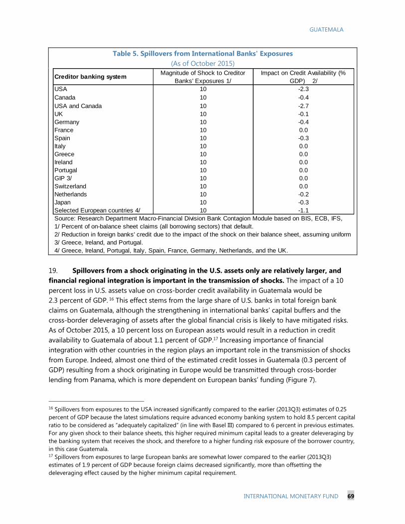
GUATEMALA
INTERNATIONAL MONETARY FUND 69
Table 5. Spillovers from International Banks' Exposures
(As of October 2015)
19. Spillovers from a shock originating in the U.S. assets only are relatively larger, and
financial regional integration is important in the transmission of shocks. The impact of a 10
percent loss in U.S. assets value on cross-border credit availability in Guatemala would be
2.3 percent of GDP. 16 This effect stems from the large share of U.S. banks in total foreign bank
claims on Guatemala, although the strengthening in international banks’ capital buffers and the
cross-border deleveraging of assets after the global financial crisis is likely to have mitigated risks.
As of October 2015, a 10 percent loss on European assets would result in a reduction in credit
availability to Guatemala of about 1.1 percent of GDP.17 Increasing importance of financial
integration with other countries in the region plays an important role in the transmission of shocks
from Europe. Indeed, almost one third of the estimated credit losses in Guatemala (0.3 percent of
GDP) resulting from a shock originating in Europe would be transmitted through cross-border
lending from Panama, which is more dependent on European banks’ funding (Figure 7).
16 Spillovers from exposures to the USA increased significantly compared to the earlier (2013Q3) estimates of 0.25
percent of GDP because the latest simulations require advanced economy banking system to hold 8.5 percent capital
ratio to be considered as “adequately capitalized” (in line with Basel III) compared to 6 percent in previous estimates.
For any given shock to their balance sheets, this higher required minimum capital leads to a greater deleveraging by
the banking system that receives the shock, and therefore to a higher funding risk exposure of the borrower country,
in this case Guatemala. 17 Spillovers from exposures to large European banks are somewhat lower compared to the earlier (2013Q3)
estimates of 1.9 percent of GDP because foreign claims decreased significantly, more than offsetting the
deleveraging effect caused by the higher minimum capital requirement.
USA 10 -2.3
Canada 10 -0.4
USA and Canada 10 -2.7
UK 10 -0.1
Germany 10 -0.4
France 10 0.0
Spain 10 -0.3
Italy 10 0.0
Greece 10 0.0
Ireland 10 0.0
Portugal 10 0.0
GIP 3/ 10 0.0
Switzerland 10 0.0
Netherlands 10 -0.2
Japan 10 -0.3
Selected European countries 4/ 10 -1.1
1/ Percent of on-balance sheet claims (all borrowing sectors) that default.
3/ Greece, Ireland, and Portugal.
4/ Greece, Ireland, Portugal, Italy, Spain, France, Germany, Netherlands, and the UK.
2/ Reduction in foreign banks' credit due to the impact of the shock on their balance sheet, assuming uniform
Creditor banking system Magnitude of Shock to Creditor
Banks' Exposures 1/
Impact on Credit Availability (%
GDP) 2/
Source: Research Department Macro-Financial Division Bank Contagion Module based on BIS, ECB, IFS,
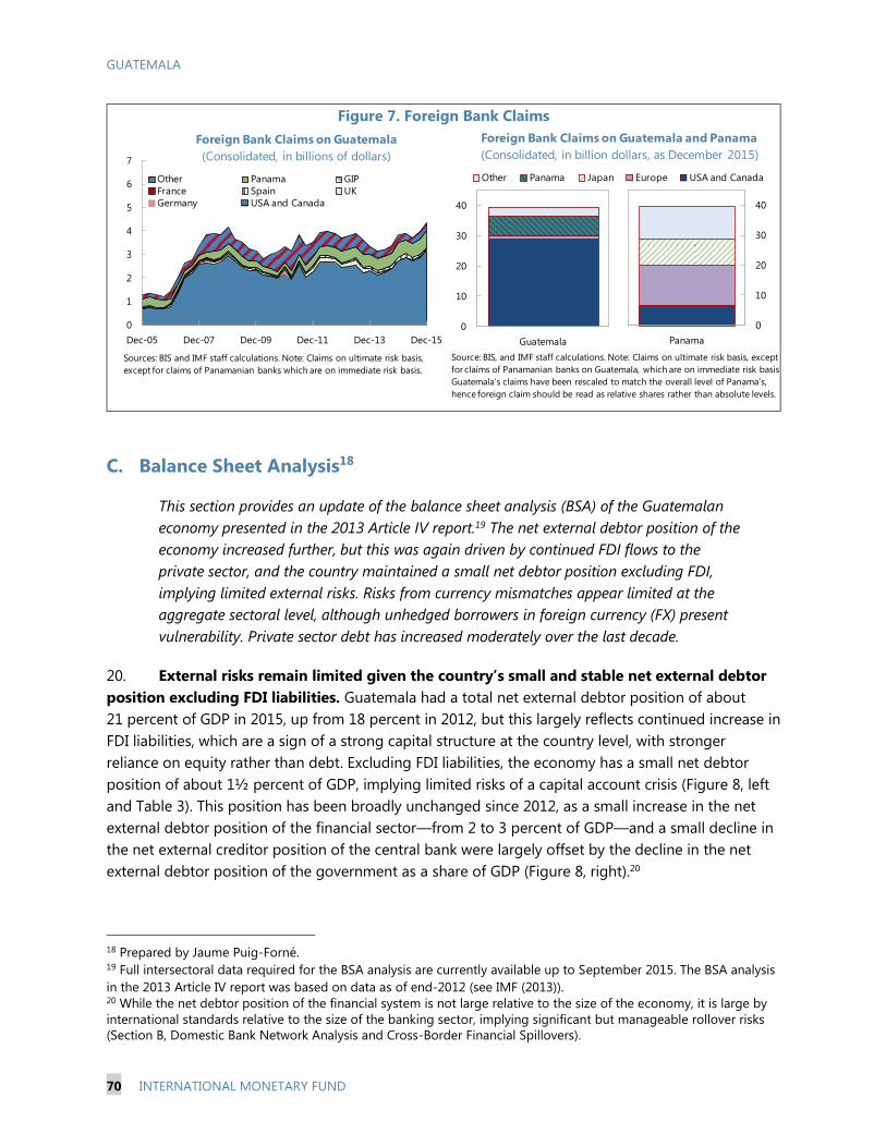
GUATEMALA
70 INTERNATIONAL MONETARY FUND
Figure 7. Foreign Bank Claims
C. Balance Sheet Analysis18
This section provides an update of the balance sheet analysis (BSA) of the Guatemalan
economy presented in the 2013 Article IV report.19 The net external debtor position of the
economy increased further, but this was again driven by continued FDI flows to the
private sector, and the country maintained a small net debtor position excluding FDI,
implying limited external risks. Risks from currency mismatches appear limited at the
aggregate sectoral level, although unhedged borrowers in foreign currency (FX) present
vulnerability. Private sector debt has increased moderately over the last decade.
20. External risks remain limited given the country’s small and stable net external debtor
position excluding FDI liabilities. Guatemala had a total net external debtor position of about
21 percent of GDP in 2015, up from 18 percent in 2012, but this largely reflects continued increase in
FDI liabilities, which are a sign of a strong capital structure at the country level, with stronger
reliance on equity rather than debt. Excluding FDI liabilities, the economy has a small net debtor
position of about 1½ percent of GDP, implying limited risks of a capital account crisis (Figure 8, left
and Table 3). This position has been broadly unchanged since 2012, as a small increase in the net
external debtor position of the financial sector—from 2 to 3 percent of GDP—and a small decline in
the net external creditor position of the central bank were largely offset by the decline in the net
external debtor position of the government as a share of GDP (Figure 8, right).20
18 Prepared by Jaume Puig-Forné. 19 Full intersectoral data required for the BSA analysis are currently available up to September 2015. The BSA analysis
in the 2013 Article IV report was based on data as of end-2012 (see IMF (2013)). 20 While the net debtor position of the financial system is not large relative to the size of the economy, it is large by
international standards relative to the size of the banking sector, implying significant but manageable rollover risks
(Section B, Domestic Bank Network Analysis and Cross-Border Financial Spillovers).
0
10
20
30
40
Guatemala
Other Panama Japan Europe USA and Canada
Foreign Bank Claims on Guatemala and Panama
(Consolidated, in billion dollars, as December 2015)
Source: BIS, and IMF staff calculations. Note: Claims on ultimate risk basis, except
for claims of Panamanian banks on Guatemala, which are on immediate risk basis.
Guatemala's claims have been rescaled to match the overall level of Panama's,
hence foreign claim should be read as relative shares rather than absolute levels.
0
10
20
30
40
Panama
0
1
2
3
4
5
6
7
Dec-05 Dec-07 Dec-09 Dec-11 Dec-13 Dec-15
Other Panama GIP
France Spain UK
Germany USA and Canada
Foreign Bank Claims on Guatemala
(Consolidated, in billions of dollars)
Sources: BIS and IMF staff calculations. Note: Claims on ultimate risk basis,
except for claims of Panamanian banks which are on immediate risk basis.

GUATEMALA
INTERNATIONAL MONETARY FUND 71
Figure 8. Net External FDI and Debt Positions
21. Notwithstanding limited currency mismatches at the aggregate level, the rising share
of FX bank credit highlights possible risks from unhedged borrowers. Currency mismatches by
sector were little changed over the last few years. Despite a small decline in reserves of the central
bank in percent of GDP, the net negative FX position of the consolidated public sector declined
slightly from about 3 percent to about 2¼ percent of GPD since 2012, driven by the decline in
external debt of the central government as a share of GDP (Table 6). The net positive FX position of
the financial sector increased slightly from about ½ percent of GDP in 2012 to about 1 percent in
2015, as banks continued channeling additional external financing into domestic credit in FX. The
non-financial private sector maintained a balanced net FX position—excluding FDI liabilities—with
foreign assets broadly offsetting the sector’s small net FX debtor position vis-à-vis banks (Tables 6
and A1). At the same time, the rising share of credit in FX over the last few years highlights possible
risks from unhedged borrowers (Section A of this note), although the concentration of such credit in
the corporate sector, especially large corporations that are more likely to have natural hedges
through export revenues, appears to be a risk-mitigating factor (Figure 9).
Figure 9. Bank Credit
Source: National authorities and Fund staff estimates.
-30
-20
-10
0
10
2007 2012 2015
Net FDI liabilities Net external debt position Total net external position
Sources: National authorities and Fund staff estimates.
Guatemala. Net External FDI and Debt Positions
(Percent of GDP)
-20
-10
0
10
20
2007 2012 2015
Central Bank NFPS Financial Sector Non-financial private sector Economy
Sources: National authorities and Fund staff estimates.
Guatemala. Net External Debt Position by Sector
(Percent of GDP)
0
10
20
30
40
50
60
70
Dec-05 Dec-07 Dec-09 Dec-11 Dec-13 Dec-15
Credit in FX (in percent of total)
Private sector
NFCs
HHs
0
10
20
30
40
50
60
70
80
90
100
Dec-05 Dec-07 Dec-09 Dec-11 Dec-13 Dec-15
Microcredit, FX
Microcredit, DC
SMEs, FX
SMEs, DC
Corporations, FX
Corporations, DC
Mortgages, FX
Mortgages, DC
Consumer, FX
Consumer, DC
Bank credit by sector (percent of total)
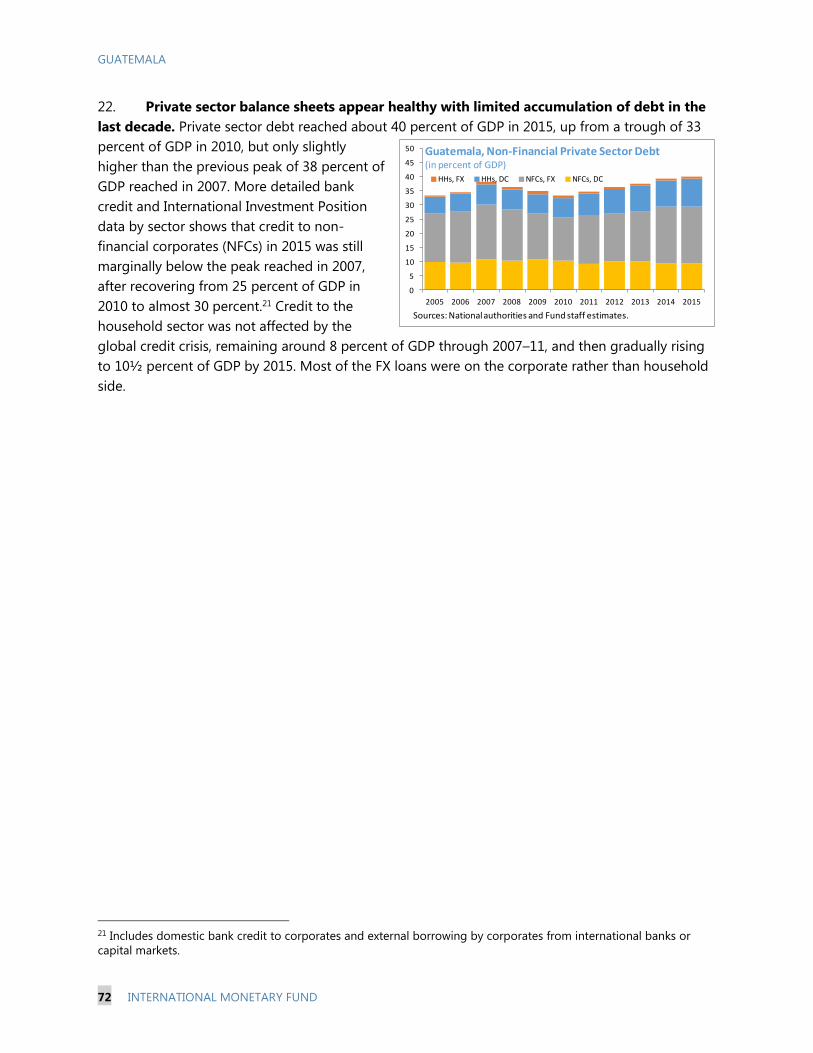
GUATEMALA
72 INTERNATIONAL MONETARY FUND
22. Private sector balance sheets appear healthy with limited accumulation of debt in the
last decade. Private sector debt reached about 40 percent of GDP in 2015, up from a trough of 33
percent of GDP in 2010, but only slightly
higher than the previous peak of 38 percent of
GDP reached in 2007. More detailed bank
credit and International Investment Position
data by sector shows that credit to non-
financial corporates (NFCs) in 2015 was still
marginally below the peak reached in 2007,
after recovering from 25 percent of GDP in
2010 to almost 30 percent.21 Credit to the
household sector was not affected by the
global credit crisis, remaining around 8 percent of GDP through 2007–11, and then gradually rising
to 10½ percent of GDP by 2015. Most of the FX loans were on the corporate rather than household
side.
21 Includes domestic bank credit to corporates and external borrowing by corporates from international banks or
capital markets.
0
5
10
15
20
25
30
35
40
45
50
2005 2006 2007 2008 2009 2010 2011 2012 2013 2014 2015
HHs, FX HHs, DC NFCs, FX NFCs, DC
Guatemala, Non-Financial Private Sector Debt (in percent of GDP)
Sources: National authorities and Fund staff estimates.

GUATEMALA
INTERNATIONAL MONETARY FUND 73
Table 6. External and Foreign Currency Positions
D. Dynamic Macro Financial Linkages22
This section simulates the effect of financial shocks on the real economy using the IMF
Flexible System of Global Models. Results indicate that the monetary stimulus injected in
2015 could continue working through the economy this year or even in the next two
years and peak in 2018 if the pass-through proves to be slow but persistent. Enhanced
competition in the banking sector resulting in lower interest rate margin, as well as lower
collateral requirements could positively and significantly contribute to economic growth,
while an exchange rate shock could take a toll on growth through increased NPLs and
market risk premia.
23. We used the IMF’s Flexible System of Global Models (FSGM) to simulate the effect of
various financial shocks on macroeconomic variables. The model was developed by the
Economic Modeling Division of the IMF’s Research department for policy analysis (Andrle and
22 Prepared by Valentina Flamini, Benjamin Hunt, and Keiko Honjo.
Central Bank
Non-financial
Public Sector Public Sector Financial Sector
Non-financial
Private Sector Economy
September 2015
Gross External Assets 12.4 0.0 12.4 5.1 10.7 28.1
Gross External Liabilities 0.9 11.7 12.6 8.0 28.1 48.8
Net External Position 11.5 -11.7 -0.2 -2.9 -17.5 -20.6
Net External Debt Position 1/ 11.5 -11.7 -0.2 -2.9 1.6 -1.6
Gross FC Assets 12.3 0.1 12.4 21.2 22.1 55.7
Gross FC Liabilities 1.5 13.2 14.7 20.4 41.1 76.1
Net FC Position 10.8 -13.1 -2.3 0.9 -18.9 -20.4
Net FX Debt Position 1/ 10.8 -13.1 -2.3 0.9 0.1 -1.3
Gross ST FC Assets 11.8 0.1 11.9 3.7 20.2 35.8
Gross ST FC Liabilities 0.9 0.6 1.5 11.4 1.2 14.1
Net ST FC Position 10.9 -0.5 10.4 -7.7 19.0 21.7
End-2012 (In percent of GDP)
Gross External Assets 13.7 0.0 13.7 5.0 11.4 30.1
Gross External Liabilities 1.3 13.6 14.8 6.9 26.7 48.4
Net External Position 12.4 -13.6 -1.1 -1.9 -15.3 -18.3
Net External Debt Position 1/ 12.4 -13.6 -1.1 -1.9 1.3 -1.8
Gross FC Assets 13.5 0.0 13.6 19.2 22.6 55.4
Gross FC Liabilities 1.6 14.9 16.4 18.6 38.4 73.5
Net FC Position 12.0 -14.8 -2.9 0.6 -15.8 -18.0
Net FX Debt Position 1/ 12.0 -14.8 -2.9 0.6 0.8 -1.5
Gross ST FC Assets 13.4 0.0 13.4 2.6 21.0 37.0
Gross ST FC Liabilities 0.9 0.5 1.4 11.1 1.5 14.0
Net ST FC Position 12.5 -0.5 12.0 -8.5 19.5 23.0
End-2007
Gross External Assets 13.0 0.0 13.0 4.4 15.0 32.3
Gross External Liabilities 1.1 13.5 14.6 5.4 24.6 44.6
Net External Position 11.9 -13.5 -1.6 -1.0 -9.6 -12.3
Net External Debt Position 1/ 11.9 -13.5 -1.6 -1.0 2.7 0.0
Gross FC Assets 12.8 0.1 12.9 19.1 25.8 57.8
Gross FC Liabilities 0.9 15.0 15.9 16.7 37.0 69.5
Net FC Position 11.9 -14.9 -3.0 2.4 -11.2 -11.7
Net FX Debt Position 1/ 11.9 -14.9 -3.0 2.4 1.1 0.6
Gross ST FC Assets 13.4 0.1 13.5 2.0 24.4 39.9
Gross ST FC Liabilities 0.7 0.6 1.4 10.9 2.6 14.8
Net ST FC Position 12.7 -0.5 12.1 -8.9 21.8 25.1
Sources: Bank of Guatemala and Fund staff estimates.
1/ Excluding net FDI position.
GUATEMALA
74 INTERNATIONAL MONETARY FUND
others, 2015). It comprises a system of multi-region globally consistent general equilibrium models
combining micro-founded and reduced-form relationships for various economic sectors. The FSGM
has a fully articulated demand side, and the supply side features are pinned down by Cobb-Douglas
production technology. International linkages are modeled in aggregate for each country/region.
The level of public debt in each country and the resulting implications for national savings
determine the global real interest rate in the long run. The parameters of the model, except those
determining the cost of adjustment in investment, have been largely estimated from the data using
a range of empirical techniques. Real GDP is determined by the sum of the components of demand
in the short run and the level of potential output in the long run. The households’ consumption-
savings decisions are explicitly micro founded as are firms’ investment decisions. The OLG
formulation of the consumption block gives the model important non-Ricardian properties, whereby
national savings are endogenously determined given the level of government debt. Government
absorption is determined exogenously, while imports and exports are specified with reduced-form
models.
24. Transmission of financial shocks to the real economy takes place through changes in
interest rates and risk premia. All interest rates are related to the risk-free interest rate, whose
closest parallel is the monetary policy rate, from which they deviate because of risk premia or
different maturities. The model includes several risk premia: one for the sovereign (which applies to
the entire domestic economy), one that applies to both domestic households and firms, one that
applies only to firms, and one that applies to the currency (or country). The expectations theory of
the term structure determines the 10-year interest rates and there is an additional term premium.
Interest rates related to consumption, investment, and holding of government debt and net foreign
assets are weighted averages of the 1- and 10-year nominal interest rates. The exchange rate in the
short run is determined via the uncovered interest parity condition, while in the long run it adjusts to
ensure external stability given households desired holdings of net foreign assets.
25. We simulate 4 scenarios which capture the macro-economic impact of shocks to
monetary policy rate, the exchange rate and market premia, lending margins, and collateral
requirements. The first scenario simulates an expansionary monetary policy shock, modeled as a
100 basis points cut in the monetary policy rate, both under full pass-through and under a slower,
but more persistent transmission to lending rates (Panels 1 and 2 in figure below); the second
simulation looks at currency depreciations of 5 and 20 percent that assumes a non-linear reaction in
market risk premia of 25 and 300 basis points (bp) respectively (Panels 3 and 4); the third scenario
considers a reduction in bank lending margins resulting in a reduction in market risk premia of 100
basis points (Panel 5); and the fourth simulates a decrease in collateral requirements, which
facilitates higher credit growth that is partially financed by higher foreign borrowing (Panel 6). Aside
from nonlinearities that can arise owing to the zero lower bound on nominal interest rates, the
model is symmetric and roughly linear; therefore, the simulated shocks can be scaled up or down to
consider scenarios of different magnitudes.
26. Results indicate that the recent 100 basis points cut in the monetary policy rate could
increase GDP substantially this year or even in the next two years. Specifically, if fully passed
GUATEMALA
INTERNATIONAL MONETARY FUND 75
through to domestic lending rates, the monetary impulse provided during 2015 (a cumulative rate
cut of 100 basis points to 3 percent amid declining inflation) could increase GDP in 2016 by almost
0.4 percentage points relative to the baseline in the absence of such stimulus due to both higher
domestic absorption and export demand. The latter effect is induced by a depreciation of the
quetzal following lower real interest rates compared to foreign rates. However, the policy rate
signaling function in Guatemala is constrained by weaknesses in the transmission from the monetary
policy rate to bank lending rates (and ultimately to prices and output). Under a slower pass-through
scenario, where only 1/3 of the impulse is passed to lending rates, the resulting increase in GDP in
2016 would be only 0.1 percent, but the delayed, more persistent impulse would increase GDP by
0.2 percent in the medium term (2017–2019) with a peak impact in 2018.
27. Conversely, a large currency depreciation could decrease output by up to 1 ½ percent
in the short and medium term, through its effect on NPLs and decreased risk appetite. In
scenario 2, a depreciation of the quetzal triggers an increase in market premia due to higher NPLs in
the context of the high degree of credit dollarization to un-hedged borrowers (40 percent of total
credit). The risk premium reaction to the depreciation is modeled as nonlinear, since defaulting
loans—and with them banks’ risk aversion—are likely to increase more than proportionally with the
extent of the depreciation. Hence, a 5 percent depreciation/20 bp increase in risk premia results in a
real GDP contraction of about 0.2 percent in the medium term. Conversely, under a 20 percent
depreciation/300 bp increase in risk premia, GDP declines by up to 1 ½ percentage points three
years after the FX shock as household consumption and private investment shrink. In both scenarios,
the short-term effect is a one-year boost to real GDP as following the depreciation exports increase
sufficiently to offset the adverse impact on domestic demand from higher risk premia.
28. Increasing efficiency and competition in the banking sector could raise GDP by up to 2
percent in the medium term. At about 8 percent, banks spreads are relatively high in Guatemala,
which is a constraint for widespread access to credit and financial inclusion. In scenario 3, we
simulate a decrease in banks’ net interest rate spreads which translates into a 100bp permanent
reduction in market risk premia. Lower rates increase both private investment and household
consumption expenditure, fostering domestic absorption. The resulting increase in inflation triggers
a policy rate increase that produces an appreciation of the quetzal and lowers exports. The net effect
on GDP is positive and persistent, with the increase ranging from less than ½ percent in the first
year to more than 2 percent after six years.

GUATEMALA
76 INTERNATIONAL MONETARY FUND
Figure 10. FSGM Model Simulations of Macro Financial Linkages
(Percent difference from baseline)
0
0.1
0.2
0.3
0.4
t t+1 t+2 t+3 t+4 t+5 t+6
GDP
CPI inflation
Core CPI inflation
Monetary Policy Impulse
(100 bps reduction)
0
0.1
0.2
0.3
0.4
t t+1 t+2 t+3 t+4 t+5 t+6
GDP
Core CPI inflation
CPI inflation
Monetary Policy Impulse
(100 bps reduction, slow pass-through)
-12
-10
-8
-6
-4
-2
0
2
4
6
8
t t+1 t+2 t+3 t+4 t+5 t+6
GDP Consumption
Investment CA
FX Depreciation
(20%, 300 bps increase in Market Risk Premium)
-2
0
2
4
6
8
10
t t+1 t+2 t+3 t+4 t+5 t+6
Output gap
GDP
Consumption
Investment
CA
Collateral Requirements
(1/2 cut)
-4
-2
0
2
4
6
8
10
12
14
16
t t+1 t+2 t+3 t+4 t+5 t+6
GDP
Consumption
Investment
CA
Interest Rate Margins
(100 bp decrease)
-2
-1.5
-1
-0.5
0
0.5
1
1.5
t t+1 t+2 t+3 t+4 t+5 t+6
GDP Consumption
Investment CA
FX Depreciation
(5%, 25 bps increase in Market Risk Premium)
Source: Staff estimates based on IMF/RES FSGM.
Note: All variables are expressed in real terms.

GUATEMALA
INTERNATIONAL MONETARY FUND 77
29. Reducing collateral requirements would yield a medium term boost to GDP similar to
improvements in bank efficiency. Effective average collateral-to-loan ratio of 157 percent as of
2010 is moderate by regional standards.23 However, reducing collateral requirements in the longer
run could help stimulate growth. In scenario 4, permanently halving collateral requirements is
assumed to bring about a 5 percent of GDP increase in domestic credit, slightly less than half of
which would be financed by domestic excess liquidity and the remaining by an increase in foreign
liabilities. Similarly to the effect of lower margins, this would increase domestic absorption while
slightly depressing exports. The increase in private investment would also accumulate into a higher
stock of private capital, which contributes to a persistent increase in both actual and potential
output. As the latter adjusts more gradually, output rises above potential and a moderate positive
output gap opens up. The overall medium term increase in GDP ranges from 0.3 percent in the first
year to over 1 ¾ percent in the sixth.
23 Regulatory limits require that credits may not exceed 70% of the value of the collateral or 80% of the value of
mortgage guarantees. However, the effective collateral-to-loan ratio reported by the companies in the Enterprise
Survey is higher since the ratio reflects the remaining maturity of the loans (the ratio increases as the loan gets closer
to maturity and a portion of the loan is repaid).

GUATEMALA
78 INTERNATIONAL MONETARY FUND
References
Allen, Mark, Christoph Rosenberg, Christian Keller, Brad Setser and Nouriel Roubini, 2002, “A Balance
Sheet Approach to Financial Crisis,” IMF Working Paper 02/210 (Washington: International
Monetary Fund).
Amo-Yartey, Charles, 2012, “Barbados: Sectoral Balance Sheet Mismatches and Macroeconomic
Vulnerabilities,” IMF Working Paper 12/31 (Washington: International Monetary Fund).
International Monetary Fund. (2013) “Guatemala Selected Issues and Analytical Notes,” Analytical
Note IV, IMF Country Report No. 13/248.
Mathisen, Johan, and Anthony Pellechio, 2006, “Using the Balance Sheet Approach in Surveillance:
Framework, Data Sources, and Data Availability,” IMF Working Paper 06/100 (Washington:
International Monetary Fund).

Annex I. Net Intersectoral Asset and Liability Positions
Table A1. Guatemala. Net Intersectoral Asset and Liability Positions, September 2015
(in percent of GDP)
Financial Sector Nonfinancial Private Sector Rest of the World
Non-financial Central Other depository Includes non-financial
Public sector bank corporations corps and households Nonresidents
Claims Liabilities Net pos. Claims Liabilities Net pos. Claims Liabilities Net pos. Claims Liabilities Net pos. Claims Liabilities Net pos. Claims Liabilities Net pos.
Non-financial public sector 5.2 2.6 2.6 8.4 4.6 3.8 0.6 0.0 0.6 0.0 0.0 0.0 11.7 0.0 11.7
In domestic currency 5.2 2.6 2.6 7.0 4.5 2.4 0.6 0.0 0.5 0.0 0.0 0.0 0.0 0.0 0.0
In foreign currency 0.0 0.0 0.0 1.4 0.1 1.4 0.1 0.0 0.1 0.0 0.0 0.0 11.7 0.0 11.7
Central bank 2.6 5.2 -2.6 9.1 0.9 8.2 0.5 0.1 0.4 0.0 0.0 0.0 0.9 12.4 -11.5
In domestic currency 2.6 5.2 -2.6 8.1 0.9 7.2 0.5 0.1 0.4 0.0 0.0 0.0 0.5 0.1 0.3
In foreign currency 0.0 0.0 0.0 1.0 0.0 1.0 0.0 0.0 0.0 0.0 0.0 0.0 0.4 12.3 -11.8
Other depository corporations 4.8 8.4 -3.6 0.9 9.1 -8.2 1.0 3.2 -2.2 50.5 35.9 14.6 8.0 5.0 3.0
In domestic currency 4.7 7.0 -2.2 0.9 8.1 -7.2 0.5 2.8 -2.3 39.3 23.0 16.2 0.0 0.1 -0.1
In foreign currency 0.1 1.4 -1.4 0.0 1.0 -1.0 0.5 0.4 0.0 11.3 12.9 -1.6 8.0 4.9 3.0
Other financial corporations 0.0 0.6 -0.6 0.1 0.5 -0.4 3.2 1.0 2.2 1.0 0.6 0.4 0.0 0.0 0.0
In domestic currency 0.0 0.6 -0.5 0.1 0.5 -0.4 2.8 0.5 2.3 0.8 0.5 0.3 0.0 0.0 0.0
In foreign currency 0.0 0.1 -0.1 0.0 0.0 0.0 0.4 0.5 0.0 0.2 0.1 0.1 0.0 0.0 0.0
Nonfinancial private sector 0.0 0.0 0.0 0.0 0.0 0.0 35.9 50.5 -14.6 0.6 1.0 -0.4 28.1 10.7 17.5
In domestic currency 0.0 0.0 0.0 0.0 0.0 0.0 23.0 39.3 -16.2 0.5 0.8 -0.3 0.0 0.0 0.0
In foreign currency 0.0 0.0 0.0 0.0 0.0 0.0 12.9 11.3 1.6 0.1 0.2 -0.1 28.1 10.7 17.5
Rest of the world 0.0 11.7 -11.7 12.4 0.9 11.5 5.0 8.0 -3.0 0.0 0.0 0.0 10.7 28.1 -17.5
In domestic currency 0.0 0.0 0.0 0.1 0.5 -0.3 0.1 0.0 0.1 0.0 0.0 0.0 0.0 0.0 0.0
In foreign currency 0.0 11.7 -11.7 12.3 0.4 11.8 4.9 8.0 -3.0 0.0 0.0 0.0 10.7 28.1 -17.5
Total 7.4 25.9 -18.5 18.6 13.2 5.4 61.6 65.0 -3.4 2.6 4.3 -1.7 62.2 64.6 -2.4 48.8 28.1 20.6
in domestic currency 7.4 12.7 -5.4 6.3 11.7 -5.4 41.0 45.2 -4.2 2.0 3.7 -1.7 40.1 23.5 16.6 0.5 0.2 0.3
in foreign currency 0.1 13.2 -13.1 12.3 1.5 10.8 20.6 19.8 0.8 0.6 0.6 0.0 22.1 41.1 -18.9 48.3 27.9 20.4
Sources: Standardized Report Forms for Monetary and Financial Data, International Investment Position, and IMF staff estimates.
Public sector
Other financial
corporationsHolder of liability
(creditor)
Issuer of liability (debtor)
GU
ATEM
ALA
INTER
NA
TIO
NA
L MO
NETA
RY F
UN
D
79

GUATEMALA
80 INTERNATIONAL MONETARY FUND
Table A2. Guatemala: Gross Financial Assets and Liabilities of Economic Sectors (Percent of GDP)
Sources: National authorities; and Fund staff estimates.
0
5
10
15
20
25Central Bank
2007 2015-30
-20
-10
0
10
20
30
40
50Non-Financial Public Sector
2007 2015
-10
0
10
20
30
40
50
60
70
80Financial Sector
Gross Assets Gross Liabilities Net
2007 2015-10
0
10
20
30
40
50
60
70Private Sector
2007 2015
GUATEMALA
INTERNATIONAL MONETARY FUND 81
MACRO FINANCIAL LINKAGES: FINANCIAL
DEVELOPMENT AND INCLUSION
A. Financial Development in Guatemala1
This section examines the current state of financial development in Guatemala, as well as
the implications for potential growth and stability from further financial deepening.
Guatemala lags its regional peers on financial development, in particular, on markets.
However, it overperforms the level of development consistent with its macroeconomic
fundamentals. Hence, while at the moment there are no indications of a significant risk
build up, further financial development should proceed with caution. In the longer term,
as fundamentals continue to evolve, Guatemala could reap further benefits from financial
development in terms of growth and stability, provided there is adequate regulatory
oversight to prevent excesses. However, care should be taken in not promoting excessive
market development when financial institutions are underdeveloped. Laying out strong
legal and institutional foundations will be important for supporting healthy financial
deepening.
Financial Development: Where Does Guatemala Stand?
1. Guatemala’s financial development was assessed using a comprehensive index.
Financial development has proven difficult to measure. Typical proxies in the literature such as the
ratio of private credit to GDP and, to a lesser extent, stock market capitalization are too narrow to
capture the broad spectrum of financial sector activities. To better capture different facets of
financial development, we employ a comprehensive and broad-based index covering 123 countries
for the period 1995–2013 (see Appendix 1 and Heng et al (2015) for details). The index contains two
major components: financial institutions and financial markets. Each component is broken down into
access, depth, and efficiency sub-components. These sub-components, in turn, are constructed
based on a number of underlying variables that track development in each area.
2. Guatemala’s financial development has improved only marginally over the past
decade, and remains low, compared to the regional peers. The small improvements came from
growth in financial institutions, in particular, better institutional access and improved efficiency. In
contrast, improvements in market development during the 90s were reversed in the 2000s. Overall,
Guatemala continues to lag behind its regional and emerging market peers on many dimensions. In
particular, it lags other EM groups on all of the subcomponents of financial market development. It
is also behind other EMs on some aspects of institutional development, though performance varies
by component. In fact, Guatemala compares favorably on institutional access, outperforming all
other EM country groupings. Good access reflects a wide network of ATMs and bank branches per
100,000 adults. However, the distribution of access points is not uniform (see Section B below). On
the other hand, the country lags behind other EMs on institutional efficiency, reflecting moderately
1 Prepared by Anna Ivanova and Victoria Valente
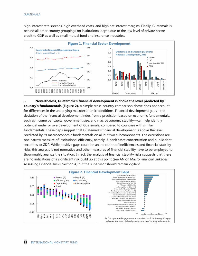
GUATEMALA
82 INTERNATIONAL MONETARY FUND
high interest rate spreads, high overhead costs, and high net interest margins. Finally, Guatemala is
behind all other country groupings on institutional depth due to the low level of private sector
credit to GDP as well as small mutual fund and insurance industries.
Figure 1. Financial Sector Development
3. Nevertheless, Guatemala’s financial development is above the level predicted by
country’s fundamentals (Figure 2). A simple cross-country comparison above does not account
for differences in the underlying macroeconomic conditions. Financial development gaps—the
deviation of the financial development index from a prediction based on economic fundamentals,
such as income per capita, government size, and macroeconomic stability—can help identify
potential under or overdevelopment of Guatemala, compared to countries with similar
fundamentals. These gaps suggest that Guatemala’s financial development is above the level
predicted by its macroeconomic fundamentals on all but two subcomponents. The exceptions are
one narrow measure of institutional efficiency, namely, 3-bank asset concentration and public debt
securities to GDP. While positive gaps could be an indication of inefficiencies and financial stability
risks, this analysis is not normative and other measures of financial stability have to be employed to
thouroughly analyze the situation. In fact, the analysis of financial stability risks suggests that there
are no indications of a significant risk build up at this point (see AN on Macro Financial Linkages:
Assessing Financial Risks, Section A) but the supervisor should remain vigilant.
Figure 2. Financial Development Gaps
1/ The signs on the gaps were harmonized such that a negative gap
indicates low level of development compared to the fundamentals.
0.00
0.01
0.02
0.03
0.04
0.05
0.0
0.1
0.2
0.3
0.4
1995
1996
1997
1998
1999
2000
2001
2002
2003
2004
2005
2006
2007
2008
2009
2010
2011
2012
2013
Total index
Financial institutions
Financial markets (rhs)
Guatemala: Financial Development Index
(Index, highest level = 1)
0.0
0.2
0.4
0.6
0.8
1.0
1.2
1.4
To
tal
To
tal
Access
Dep
th
Eff
icie
ncy
To
tal
Access
Dep
th
Eff
icie
ncy
Overall Institutions Markets
EM Asia
LAC
Non Asia/LAC EM
GTM
Guatemala and Emerging Markets:
Financial Development, 2013
-0.10
-0.05
0.00
0.05
0.10
PA
N
HN
D
PER
BO
L
BR
A
GTM
EC
U
SLV
CO
L
MEX
NIC
VEN
PR
Y
CH
L
CR
I
JAM
DO
M
UR
Y
Access (FI) Depth (FI)
Efficiency (FI) Access (FM)
Depth (FM) Efficiency (FM)
Total
-20 0 20 40 60
3 Bank Asset Concentration (%)
Public Debt Securities / GDP (%)
Overhead Costs / Total Assets (%)
Securities of non-financial sector in % of GDP
Interest rate spread
Bank net interest margin (%)
Market capitalization excluding top 10
Securities of financial sector in % of GDP
Insurance Company Assets / GDP (%)
Domestic credit to private sector (% of GDP)
Non-Interest Income / Total income (%)
Domestic Bank Deposits / GDP (%)
Market capitalization (% of GDP)
ATMs, per 100,000 adults
Mutual Fund Assets / GDP (%)
Stocks traded, turnover ratio (%)
Commercial Banks, per 100,000 Adults
Stocks traded, total value (% of GDP)
Total number of issuers of debt
Gaps with respect to fundamentals
GUATEMALA
INTERNATIONAL MONETARY FUND 83
The Potential for Raising Growth and Stability through Further Financial Deepening in
Guatemala
4. There is a non-linear relationship between growth and stability on the one hand and
financial development on the other hand. Financial development gaps do not address the
question of the optimal level of financial development in terms of growth and stability. To explore
this question, we examine the relationships between financial development and growth as well as
financial development and stability (see Heng et al., 2015). We find that these relationships are
nonlinear. In other words, the benefits from financial development are rising at the early stages of
development as resources are increasingly channeled into productive uses. However, there is a
turning point beyond which the positive growth benefits diminish. Similarly, at the early stages,
financial development can help reduce instability, for example, by providing insurance services, but
these benefits also start to diminish after a certain point. The turning points likely reflect the fact
that large financial systems can eventually divert resources from more productive activities, while
excessive borrowing and risk-taking by financial institutions can lead to increased instability and
lower long-term growth. Indeed, the inverted U-shaped relationship with growth is driven by the
depth of financial institutions, or a measure of size. Access and efficiency, on the other hand, yield
unambiguously increasing benefits to growth, although with potential stability costs as reduced
bank profitability may encourage risk-taking. Lastly, too much market development at the early
stages of institutional development may have negative implications for stability. One reason for this
could be increased market volatility, which may more easily set in when financial institutions are not
strong enough to help guard against shocks. For similar levels of development, however, institutions
and markets are complementary for growth and stability.
5. Guatemala has not yet reached the levels of institutional and market development that
yield maximum benefits to growth and stability. In Latin America and the Caribbean, Brazil and
Chile are closest to reaping the maximum benefits (Figure 3). Guatemala, in contrast, is still far away
from reaping the maximum benefits to growth and stability, in particular, in terms of financial
market development. Note that these estimates stem from a partial analysis that assumes that all
other growth determinants (such as income level, inflation, government size etc.) are held constant
while financial development is consistent with the level of macroeconomic fundamentals. Thus, in
the longer term, reaping maximum benefits from financial development for growth and stability
would also require adjusting Guatemala’s macroeconomic fundamentals, which in turn would
support further development of the financial systems. This is an interactive process whereby
financial systems are shaped by fundamentals, and fundamentals evolve partly as a function of more
developed financial systems. Estimates should, however, be interpreted with caution since it is
difficult to disentangle causality in econometric terms, even though instrumental variables were
used to address potential endogeneity issues.2
2 We use system GMM estimation (Arellano and Bover, 1995; Blundell and Bond, 1998) to address the dynamic
dependence of our variables of interest and potential endogeneity of control variables. We also employ additional
instrumental variables used in the literature, namely, rule of law (Kaufmann, Kraay and Mastruzzi 2010) and a set of
dummies for the country’s legal origin (La Porta, Lopez-de-Silanes and Shleifer 2008).
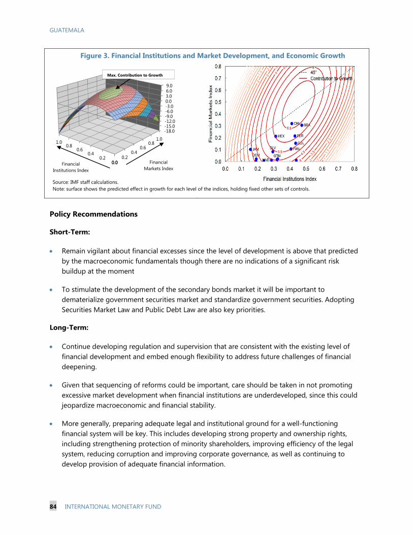
GUATEMALA
84 INTERNATIONAL MONETARY FUND
Figure 3. Financial Institutions and Market Development, and Economic Growth
Policy Recommendations
Short-Term:
Remain vigilant about financial excesses since the level of development is above that predicted
by the macroeconomic fundamentals though there are no indications of a significant risk
buildup at the moment
To stimulate the development of the secondary bonds market it will be important to
dematerialize government securities market and standardize government securities. Adopting
Securities Market Law and Public Debt Law are also key priorities.
Long-Term:
Continue developing regulation and supervision that are consistent with the existing level of
financial development and embed enough flexibility to address future challenges of financial
deepening.
Given that sequencing of reforms could be important, care should be taken in not promoting
excessive market development when financial institutions are underdeveloped, since this could
jeopardize macroeconomic and financial stability.
More generally, preparing adequate legal and institutional ground for a well-functioning
financial system will be key. This includes developing strong property and ownership rights,
including strengthening protection of minority shareholders, improving efficiency of the legal
system, reducing corruption and improving corporate governance, as well as continuing to
develop provision of adequate financial information.
0.00.2
0.40.6
0.81.0
-18.0-15.0-12.0-9.0-6.0-3.00.03.06.09.0
0.00.2
0.40.6
0.81.0
Financial
Markets IndexFinancial
Institutions Index
Max. Contribution to Growth
Source: IMF staff calculations.
Note: surface shows the predicted effect in growth for each level of the indices, holding fixed other sets of controls.
GUATEMALA
INTERNATIONAL MONETARY FUND 85
B. Financial Inclusion in Guatemala3
This section examines the current status of financial inclusion in Guatemala, identifies the
remaining gaps, and analyzes the impact of removing impediments to financial inclusion
on growth and inequality. Guatemala has excelled in providing physical access to
financial infrastructure but lags behind peers on creating an enabling regulatory
environment for financial inclusion and on the use of financial services by households
and firms. While low use to a large extent reflects Guatemala’s current state of economic
development, strengthening regulatory environment and reducing entry costs—with the
latter helping stimulate growth and reduce inequality—are matters of high priority. In the
longer run, creating better conditions for income growth, improving education,
particularly, of women, reducing the size of the informal economy and strengthening the
rule of law will help raise financial inclusion further.
Introduction
6. Guatemala can benefit from further financial inclusion. Financial inclusion can help
boost economic growth and reduce poverty and inequality by mobilizing savings and providing
households and firms with greater access to resources needed to finance consumption and
investment and to insure against shocks. Financial inclusion can also foster formalization of the
economy, helping, in turn, to boost government revenues and strengthen social safety nets. Given a
relatively low level of income per capita, high inequality, low savings and investment as well as high
labor informality, the benefits from further financial inclusion can be pronounced in Guatemala.
7. The note takes three separate approaches for examining different faucets of financial
inclusion and its impediments in Guatemala.4 First, an empirical approach focuses on measuring
financial inclusion, identifying financial inclusion gaps, and their underlying drivers. It is based on
composite measures of household and firm financial inclusion as well as a measure physical access
to financial infrastructure using recently updated FINDEX dataset (World Bank), Enterprise Survey
(World Bank), and Financial Access Survey (IMF). These measures help place Guatemala in a
temporal and cross-country perspective. Second, a regression analysis is employed to identify
characteristics of the individuals who use financial services (i.e. those financially-included). Third, a
novel theoretical framework is employed to identify the most binding financial sector frictions that
impede financial inclusion in Guatemala. This framework allows examining the implications of
alleviating financial frictions on inequality and growth.
3 Prepared by Noelia Camara (BBVA), Yixi Deng, Anna Ivanova, and Joyce Wong (all IMF). 4 The first and the third approaches follow closely those proposed in the IMF working paper “Financial Inclusion:
Zooming in on Latin America” by Era Dabla-Norris, Yixi Deng, Anna Ivanova, Izabela Karpowicz, Filiz Unsal, Eva
VanLeemput, and Joyce Wong.

GUATEMALA
86 INTERNATIONAL MONETARY FUND
Empirical Approach I: Cross-Country Data
A. Where Does Guatemala Stand on Financial Inclusion Compared to Peers?
8. Guatemala has excelled on physical access to financial infrastructure though access
points are concentrated around Guatemala City (Figure 4). We measure physical access by the
number of commercial bank branches and ATMs per 100,000 adults and per 1,000 square kilometers
(see the Figure 4 and Appendix 2 for details). Guatemala has made substantial progress on
improving physical access to financial infrastructure in the past decade with the number of
commercial bank branches per 100,000 adults rising from 18.8 in 2004 to 37 in 2014. In fact,
Guatemala now stands as one of the champions on physical access to financial infrastructure in Latin
America and the Caribbean (LAC) with 37 branches and 36 ATMs per 100,000 adults, outpacing LAC
averages of 24 for branches and 25 for ATMs. In addition, Guatemala has a network of bank
correspondents, which are used more widely than elsewhere in LAC.5 The distribution of access
points, however, is not uniform. Commercial bank branches are concentrated in the area
surrounding Guatemala City while banking correspondents are located in remote areas.
9. Guatemala, however, lags behind peers on creating an enabling regulatory
environment for financial inclusion. It scores below average of other emerging markets on the
Global Microscope index, which assesses the regulatory environment for financial inclusion across 12
indicators and 55 countries. This is in contrast to many LAC countries, which score well on this index
with Peru being the world champion. In 2015 Guatemala ranked relatively well on two Microscope
indicators: (i) regulation and supervision of branches and agents and (ii) requirements for non-
regulated lenders. It was on par with other LAC countries on average (though generally below
emerging Asia) on (i) regulation and supervision of deposit-taking activities, (ii) regulation and
supervision of credit portfolios, (ii) regulatory and supervisory capacity for financial inclusion, and
(iii) regulation of insurance for low income population. However, Guatemala underperformed on
other sub-components of the Global Microscope Index, including, (i) government support for
financial inclusion, largely due to the absence of a formal comprehensive financial inclusion strategy,
(ii) regulation of electronic payments, (iii) market conduct rules, (iv) grievance redress and operation
of dispute resolution, (v) credit reporting systems, and (vi) prudential regulation. The authorities,
however, are already working on addressing some of the weaknesses, including the recent adoption
of the regulation of mobile financial services and the microfinance law as well as the preparation of
the national financial inclusion strategy.
5 Banking correspondents are non-financial commercial establishments that offer basic financial services under the
name of a financial services provider, facilitating access points to the formal financial system, in particular, for low-
income customers. The establishments are spread across diverse sectors (grocery shops, gas stations, postal services,
pharmacies, etc.) as long as they are brick-and-mortar stores whose core business involves managing cash. In its
basic form, banking correspondents carry out only transactional operations (cash in, cash out) and payments but, in
some cases, they have evolved as a distribution channel for the banks’ credit, saving and insurance products. See
Camara, Tuesta, and Urbiola (2015) for details.
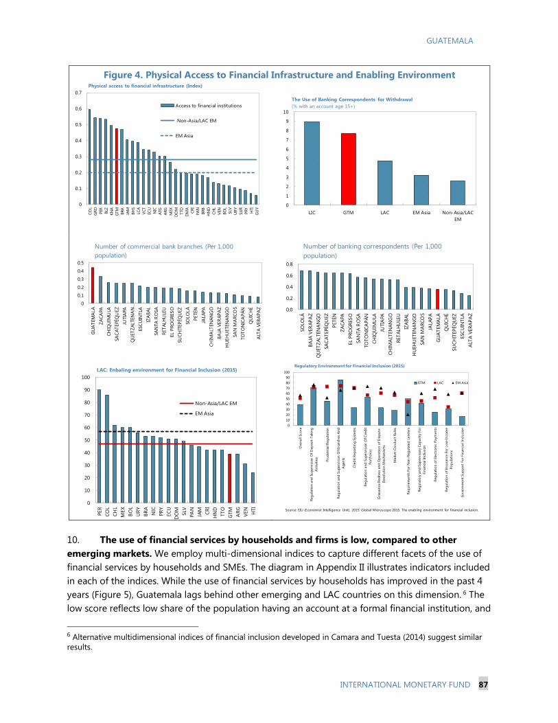
GUATEMALA
INTERNATIONAL MONETARY FUND 87
Figure 4. Physical Access to Financial Infrastructure and Enabling Environment
10. The use of financial services by households and firms is low, compared to other
emerging markets. We employ multi-dimensional indices to capture different facets of the use of
financial services by households and SMEs. The diagram in Appendix II illustrates indicators included
in each of the indices. While the use of financial services by households has improved in the past 4
years (Figure 5), Guatemala lags behind other emerging and LAC countries on this dimension. 6 The
low score reflects low share of the population having an account at a formal financial institution, and
6 Alternative multidimensional indices of financial inclusion developed in Camara and Tuesta (2014) suggest similar
results.
0
0.1
0.2
0.3
0.4
0.5
0.6
0.7C
OL
GR
D
PER
BLZ
KN
A
GTM
BRA
JAM
BH
S
LCA
VCT
ECU
NIC
ATG
ARG
MEX
DO
M
TTO
DM
A
CRI
PA
N
BRB
HN
D
CH
L
VEN
BO
L
SLV
UR
Y
SU
R
PRY
HTI
GU
Y
Physical access to financial infrastructure (Index)
Access to financial institutions
Non-Asia/LAC EM
EM Asia
0
1
2
3
4
5
6
7
8
9
10
LIC GTM LAC EM Asia Non-Asia/LAC
EM
The Use of Banking Correspondents for Withdrawal
(% with an account age 15+)
0
0.1
0.2
0.3
0.4
0.5
GU
AT
EM
ALA
ZA
CA
PA
CH
IQU
IMU
LA
SA
CA
TEPÉQ
UEZ
JUTIA
PA
QU
ET
ZA
LTEN
AN
…
ESC
UIN
TLA
IZA
BA
L
SA
NTA
RO
SA
RET
ALH
ULE
U
EL P
RO
GR
ES
O
SU
CH
ITEP
ÉQ
UEZ
SO
LO
LÁ
PETÉN
JALA
PA
CH
IMA
LTEN
AN
GO
BA
JA V
ER
AP
AZ
HU
EH
UETEN
AN
GO
SA
N M
AR
CO
S
TO
TO
NIC
AP
ÁN
QU
ICH
É
ALT
A V
ER
AP
AZ
Number of commercial bank branches (Per 1,000
population)
0.0
0.2
0.4
0.6
0.8
SO
LO
LÁ
BA
JA V
ER
AP
AZ
QU
ET
ZA
LTEN
AN
GO
SA
CA
TEPÉQ
UEZ
PETÉN
ZA
CA
PA
EL P
RO
GR
ES
O
SA
NTA
RO
SA
TO
TO
NIC
AP
ÁN
CH
IQU
IMU
LA
JUTIA
PA
CH
IMA
LTEN
AN
GO
RET
ALH
ULE
U
IZA
BA
L
HU
EH
UETEN
AN
GO
SA
N M
AR
CO
S
JALA
PA
GU
AT
EM
ALA
QU
ICH
É
SU
CH
ITEP
ÉQ
UEZ
ESC
UIN
TLA
ALT
A V
ER
AP
AZ
Number of banking correspondents (Per 1,000
population)
0
10
20
30
40
50
60
70
80
90
100
PER
CO
L
CH
L
MEX
BO
L
UR
Y
BR
A
NIC
PR
Y
EC
U
DO
M
SLV
PA
N
JAM
CR
I
HN
D
TTO
GTM
AR
G
VEN
HTI
LAC: Enbaling environment for Financial Inclusion (2015)
Non-Asia/LAC EM
EM Asia
0
10
20
30
40
50
60
70
80
90
100
Ove
rall
Sco
re
Reg
ula
tio
n a
nd
Su
perv
isio
n O
f D
ep
osi
t-Takin
g
Act
ivit
ies
Pru
den
tial R
eg
ula
tion
Reg
ula
tio
n a
nd
Su
perv
isio
n O
f B
ran
ches
And
Agen
ts
Cre
dit R
ep
ort
ing S
yst
em
s
Reg
ula
tio
n a
nd
Su
perv
isio
n O
f C
red
it
Po
rtfo
lio
s
Gri
eva
nce
Red
ress
and
Op
era
tio
n o
f D
ispu
te
Reso
luti
on M
ech
anis
ms
Mark
et
Co
nd
uct
Ru
les
Req
uir
em
ents
For
Non
-Reg
ula
ted
Lend
ers
Reg
ula
tory
an
d S
up
erv
isory
Cap
aci
ty F
or
Fin
an
cial In
clu
sion
Reg
ula
tio
n o
f Ele
ctro
nic
Paym
ents
Reg
ula
tio
n o
f In
sura
nce
Fo
r Lo
w-I
nco
me
Po
pu
latio
ns
Go
vern
men
t Sup
po
rt F
or
Fin
anci
al In
clu
sio
n
GTM LAC EM Asia
Source: EIU (Economist Intelligence Unit). 2015. Global Microscope 2015: The enabling environment for financial inclusion.
Regulatory Environment for Financial Inclusion (2015)

GUATEMALA
88 INTERNATIONAL MONETARY FUND
using ATMs, debit and credit cards. Indeed, while the share of adult population having an account at
a formal financial institution increased dramatically over the past few years – from 22 percent in
2011 to 41 percent in 2014 – it remains below that of other LAC countries on average (46.5 percent)
and even more so of emerging Asia (60.35 percent). Guatemala, however, is at par with the regional
peers on savings and borrowing from a formal financial institution. Nonetheless, informal finance
remains important with the share of population using savings clubs in 2014 as large as that saving at
a formal financial institution (12 percent versus 8 percent in LAC on average) and 20 percent of the
population reporting borrowing from family and friends, compared to only 14 percent in LAC.
Guatemala also does not compare favorably to its regional and emerging market peers on the use
of financial services by firms. This reflects low account ownership by SMEs with only 60 percent of
firms reporting having a checking or savings account, compared to a LAC average of 92 percent.
Low share of firms using banks to finance investments and working capital and somewhat high
collateral value, compared to emerging markets outside of LAC, also contribute to a lower firm
score.
Figure 5. Use of Financial Services by Households and Firms
0
0.1
0.2
0.3
0.4
0.5
0.6
0.7
CH
L
BR
A
UR
Y
CR
I
JAM
VEN
AR
G
CO
L
DO
M
MEX
PR
Y
PA
N
SLV
BO
L
BLZ
EC
U
PER
GTM
NIC
HN
D
HTI
Latin America: Index of Household Use of Financial Services,
2011-2014
2011 2014
Non-Asia/LAC EM, 2014 EM Asia, 2014
0
0.1
0.2
0.3
0.4
0.5
0.6
0.7
0.8
0.9
1
CH
L
VC
T
BR
B
BR
A
TTO
PER
GU
Y
KN
A
ATG
GR
D
DO
M
SU
R
SLV
BO
L
EC
U
VEN
CO
L
UR
Y
BH
S
BLZ
LCA
PR
Y
JAM
CR
I
GTM
DM
A
AR
G
NIC
MEX
HN
D
PA
N
Latin AmericaL Index of Firm Use of Financial Services, Various
Years
Non-Asian/LAC EM average
EM Asia
0
50
100
150
200
250
Tota
l Fir
m U
sage
index*
100
Valu
e o
f C
olla
tera
l
Need
ed f
or
a Lo
an
(% o
f th
e L
oan…
% o
f Fi
rms
With a
n
Acc
ount
% o
f Fi
rms
With
Bank
Loan
s/lin
e o
f
Cre
dit
% o
f Fi
rms
no
t
needin
g a
loan
% o
f Fi
rms
Usi
ng
Banks
to F
inance
Inve
stm
ents
% o
f Fi
rms
Iden
tify
ing
Acc
ess
/cost
of…
Work
ing C
apit
al
Bank
Fin
anci
ng
(%
)
LAC and EMs: Enterprise Use of Financial Services
(percent)
EM Asia
LAC
Non-Asia/LAC EM
GTM
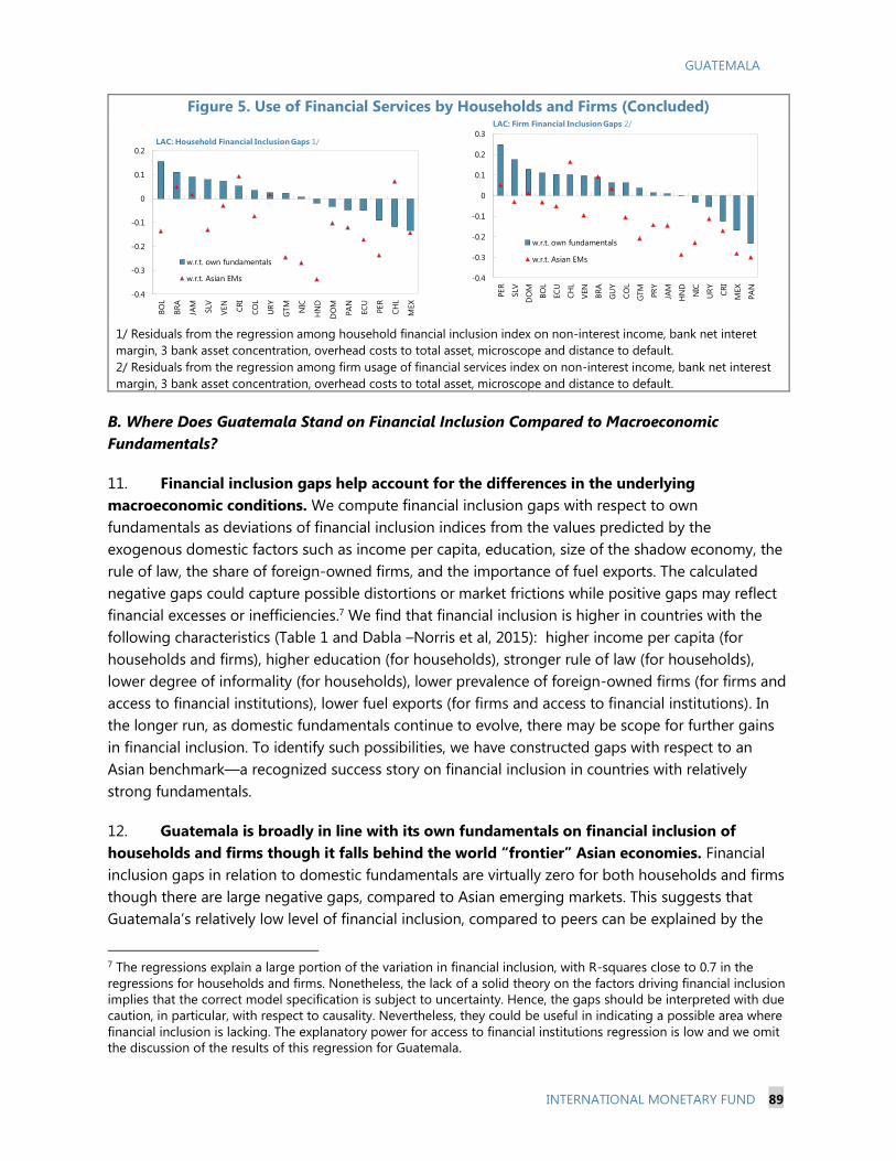
GUATEMALA
INTERNATIONAL MONETARY FUND 89
B. Where Does Guatemala Stand on Financial Inclusion Compared to Macroeconomic
Fundamentals?
11. Financial inclusion gaps help account for the differences in the underlying
macroeconomic conditions. We compute financial inclusion gaps with respect to own
fundamentals as deviations of financial inclusion indices from the values predicted by the
exogenous domestic factors such as income per capita, education, size of the shadow economy, the
rule of law, the share of foreign-owned firms, and the importance of fuel exports. The calculated
negative gaps could capture possible distortions or market frictions while positive gaps may reflect
financial excesses or inefficiencies.7 We find that financial inclusion is higher in countries with the
following characteristics (Table 1 and Dabla –Norris et al, 2015): higher income per capita (for
households and firms), higher education (for households), stronger rule of law (for households),
lower degree of informality (for households), lower prevalence of foreign-owned firms (for firms and
access to financial institutions), lower fuel exports (for firms and access to financial institutions). In
the longer run, as domestic fundamentals continue to evolve, there may be scope for further gains
in financial inclusion. To identify such possibilities, we have constructed gaps with respect to an
Asian benchmark—a recognized success story on financial inclusion in countries with relatively
strong fundamentals.
12. Guatemala is broadly in line with its own fundamentals on financial inclusion of
households and firms though it falls behind the world “frontier” Asian economies. Financial
inclusion gaps in relation to domestic fundamentals are virtually zero for both households and firms
though there are large negative gaps, compared to Asian emerging markets. This suggests that
Guatemala’s relatively low level of financial inclusion, compared to peers can be explained by the
7 The regressions explain a large portion of the variation in financial inclusion, with R-squares close to 0.7 in the
regressions for households and firms. Nonetheless, the lack of a solid theory on the factors driving financial inclusion
implies that the correct model specification is subject to uncertainty. Hence, the gaps should be interpreted with due
caution, in particular, with respect to causality. Nevertheless, they could be useful in indicating a possible area where
financial inclusion is lacking. The explanatory power for access to financial institutions regression is low and we omit
the discussion of the results of this regression for Guatemala.
Figure 5. Use of Financial Services by Households and Firms (Concluded)
1/ Residuals from the regression among household financial inclusion index on non-interest income, bank net interet
margin, 3 bank asset concentration, overhead costs to total asset, microscope and distance to default.
2/ Residuals from the regression among firm usage of financial services index on non-interest income, bank net interest
margin, 3 bank asset concentration, overhead costs to total asset, microscope and distance to default.
-0.4
-0.3
-0.2
-0.1
0
0.1
0.2
BO
L
BR
A
JAM
SLV
VEN
CR
I
CO
L
UR
Y
GTM
NIC
HN
D
DO
M
PA
N
EC
U
PER
CH
L
MEX
LAC: Household Financial Inclusion Gaps 1/
w.r.t. own fundamentals
w.r.t. Asian EMs
Sources: FINDEX, IMF staff calculations
-0.4
-0.3
-0.2
-0.1
0
0.1
0.2
0.3
PER
SLV
DO
M
BO
L
EC
U
CH
L
VEN
BR
A
GU
Y
CO
L
GTM
PR
Y
JAM
HN
D
NIC
UR
Y
CR
I
MEX
PA
N
LAC: Firm Financial Inclusion Gaps 2/
w.r.t. own fundamentals
w.r.t. Asian EMs
Sources: FINDEX, IMF staff calculations
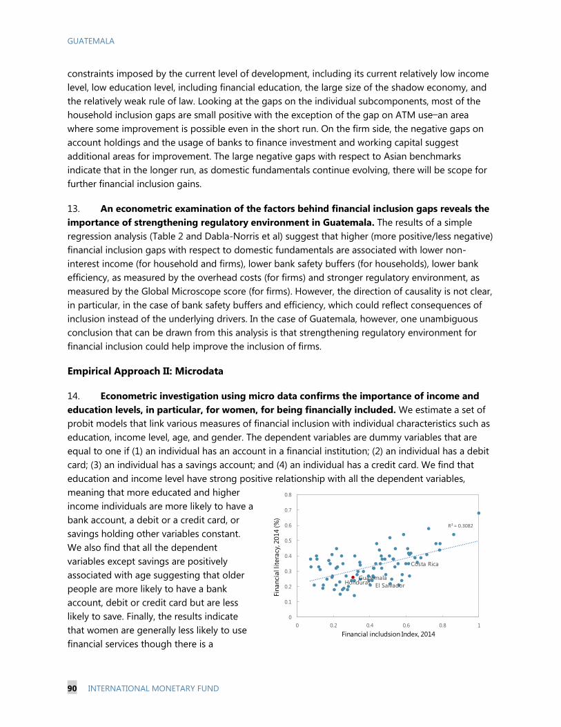
GUATEMALA
90 INTERNATIONAL MONETARY FUND
constraints imposed by the current level of development, including its current relatively low income
level, low education level, including financial education, the large size of the shadow economy, and
the relatively weak rule of law. Looking at the gaps on the individual subcomponents, most of the
household inclusion gaps are small positive with the exception of the gap on ATM use—an area
where some improvement is possible even in the short run. On the firm side, the negative gaps on
account holdings and the usage of banks to finance investment and working capital suggest
additional areas for improvement. The large negative gaps with respect to Asian benchmarks
indicate that in the longer run, as domestic fundamentals continue evolving, there will be scope for
further financial inclusion gains.
13. An econometric examination of the factors behind financial inclusion gaps reveals the
importance of strengthening regulatory environment in Guatemala. The results of a simple
regression analysis (Table 2 and Dabla-Norris et al) suggest that higher (more positive/less negative)
financial inclusion gaps with respect to domestic fundamentals are associated with lower non-
interest income (for household and firms), lower bank safety buffers (for households), lower bank
efficiency, as measured by the overhead costs (for firms) and stronger regulatory environment, as
measured by the Global Microscope score (for firms). However, the direction of causality is not clear,
in particular, in the case of bank safety buffers and efficiency, which could reflect consequences of
inclusion instead of the underlying drivers. In the case of Guatemala, however, one unambiguous
conclusion that can be drawn from this analysis is that strengthening regulatory environment for
financial inclusion could help improve the inclusion of firms.
Empirical Approach II: Microdata
14. Econometric investigation using micro data confirms the importance of income and
education levels, in particular, for women, for being financially included. We estimate a set of
probit models that link various measures of financial inclusion with individual characteristics such as
education, income level, age, and gender. The dependent variables are dummy variables that are
equal to one if (1) an individual has an account in a financial institution; (2) an individual has a debit
card; (3) an individual has a savings account; and (4) an individual has a credit card. We find that
education and income level have strong positive relationship with all the dependent variables,
meaning that more educated and higher
income individuals are more likely to have a
bank account, a debit or a credit card, or
savings holding other variables constant.
We also find that all the dependent
variables except savings are positively
associated with age suggesting that older
people are more likely to have a bank
account, debit or credit card but are less
likely to save. Finally, the results indicate
that women are generally less likely to use
financial services though there is a
Costa Rica
El Salvador
GuatemalaHonduras
R² = 0.3082
0
0.1
0.2
0.3
0.4
0.5
0.6
0.7
0.8
0 0.2 0.4 0.6 0.8 1
Financial includsion Index, 2014
Financi
al l
itera
cy, 2
014 (%
)
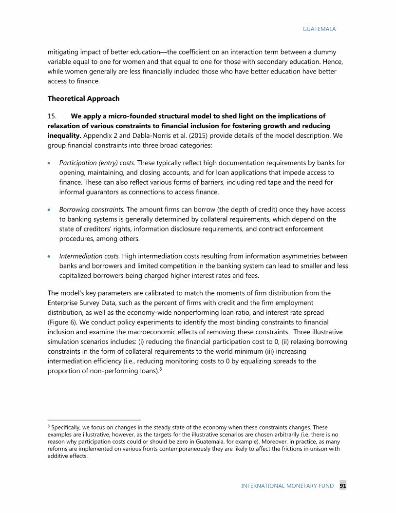
GUATEMALA
INTERNATIONAL MONETARY FUND 91
mitigating impact of better education—the coefficient on an interaction term between a dummy
variable equal to one for women and that equal to one for those with secondary education. Hence,
while women generally are less financially included those who have better education have better
access to finance.
Theoretical Approach
15. We apply a micro-founded structural model to shed light on the implications of
relaxation of various constraints to financial inclusion for fostering growth and reducing
inequality. Appendix 2 and Dabla-Norris et al. (2015) provide details of the model description. We
group financial constraints into three broad categories:
Participation (entry) costs. These typically reflect high documentation requirements by banks for
opening, maintaining, and closing accounts, and for loan applications that impede access to
finance. These can also reflect various forms of barriers, including red tape and the need for
informal guarantors as connections to access finance.
Borrowing constraints. The amount firms can borrow (the depth of credit) once they have access
to banking systems is generally determined by collateral requirements, which depend on the
state of creditors’ rights, information disclosure requirements, and contract enforcement
procedures, among others.
Intermediation costs. High intermediation costs resulting from information asymmetries between
banks and borrowers and limited competition in the banking system can lead to smaller and less
capitalized borrowers being charged higher interest rates and fees.
The model's key parameters are calibrated to match the moments of firm distribution from the
Enterprise Survey Data, such as the percent of firms with credit and the firm employment
distribution, as well as the economy-wide nonperforming loan ratio, and interest rate spread
(Figure 6). We conduct policy experiments to identify the most binding constraints to financial
inclusion and examine the macroeconomic effects of removing these constraints. Three illustrative
simulation scenarios includes: (i) reducing the financial participation cost to 0, (ii) relaxing borrowing
constraints in the form of collateral requirements to the world minimum (iii) increasing
intermediation efficiency (i.e., reducing monitoring costs to 0 by equalizing spreads to the
proportion of non-performing loans).8
8 Specifically, we focus on changes in the steady state of the economy when these constraints changes. These
examples are illustrative, however, as the targets for the illustrative scenarios are chosen arbitrarily (i.e. there is no
reason why participation costs could or should be zero in Guatemala, for example). Moreover, in practice, as many
reforms are implemented on various fronts contemporaneously they are likely to affect the frictions in unison with
additive effects.
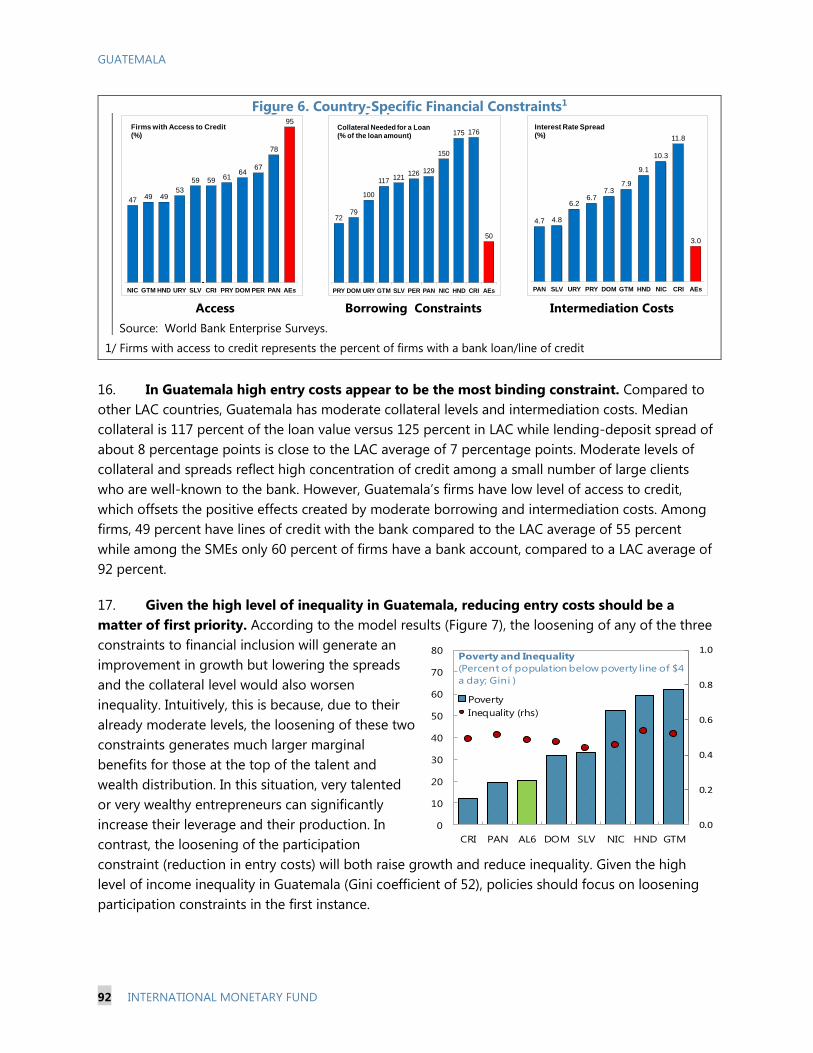
GUATEMALA
92 INTERNATIONAL MONETARY FUND
Figure 6. Country-Specific Financial Constraints1
1/ Firms with access to credit represents the percent of firms with a bank loan/line of credit
16. In Guatemala high entry costs appear to be the most binding constraint. Compared to
other LAC countries, Guatemala has moderate collateral levels and intermediation costs. Median
collateral is 117 percent of the loan value versus 125 percent in LAC while lending-deposit spread of
about 8 percentage points is close to the LAC average of 7 percentage points. Moderate levels of
collateral and spreads reflect high concentration of credit among a small number of large clients
who are well-known to the bank. However, Guatemala’s firms have low level of access to credit,
which offsets the positive effects created by moderate borrowing and intermediation costs. Among
firms, 49 percent have lines of credit with the bank compared to the LAC average of 55 percent
while among the SMEs only 60 percent of firms have a bank account, compared to a LAC average of
92 percent.
17. Given the high level of inequality in Guatemala, reducing entry costs should be a
matter of first priority. According to the model results (Figure 7), the loosening of any of the three
constraints to financial inclusion will generate an
improvement in growth but lowering the spreads
and the collateral level would also worsen
inequality. Intuitively, this is because, due to their
already moderate levels, the loosening of these two
constraints generates much larger marginal
benefits for those at the top of the talent and
wealth distribution. In this situation, very talented
or very wealthy entrepreneurs can significantly
increase their leverage and their production. In
contrast, the loosening of the participation
constraint (reduction in entry costs) will both raise growth and reduce inequality. Given the high
level of income inequality in Guatemala (Gini coefficient of 52), policies should focus on loosening
participation constraints in the first instance.
Figure 4. Country-Specific Financial Constraints
Access Borrowing Constraints Intermediation Costs
Source: World Bank Enterprise Surveys.
47 49 4953
59 59 6164
67
78
95
NIC GTM HND URY SLV CRI PRY DOM PER PAN AEs
Firms with Access to Credit(%)
7279
100
117 121126 129
150
175 176
50
PRY DOM URY GTM SLV PER PAN NIC HND CRI AEs
Collateral Needed for a Loan(% of the loan amount)
4.7 4.8
6.26.7
7.37.9
9.1
10.3
11.8
3.0
PAN SLV URY PRY DOM GTM HND NIC CRI AEs
Interest Rate Spread(%)
0.0
0.2
0.4
0.6
0.8
1.0
0
10
20
30
40
50
60
70
80
CRI PAN AL6 DOM SLV NIC HND GTM
Poverty
Inequality (rhs)
Poverty and Inequality
(Percent of population below poverty line of $4
a day; Gini )

GUATEMALA
INTERNATIONAL MONETARY FUND 93
Policy Recommendations
Short-term
Improve regulatory environment for financial inclusion, in particular, finalize and adopt the
national financial inclusion strategy, improve regulation of electronic payments, market conduct
rules, and credit reporting systems. The recently adopted mobile money regulation was an
important step and continuing developing e-money will facilitate access in remote areas.
Figure 7. Impact of Reducing Financial Constraints on GDP and Inequality
0
1
2
3
4
5
DOM SLV PAN URY NIC GTM HND PRY COL PER CRI
% p
ts c
ha
ng
e in
GD
P
Effect on GDP of making participation costs 0
0
5
10
15
20
25
COL HND SLV PER CRI PAN NIC GTM URY DOM PRY
% p
ts c
ha
ng
e in
GD
P
Effect on GDP of taking collateral to world minimum
0
1
2
3
4
5
6
7
PRY PER CRI NIC HND URY GTM DOM PAN COL SLV
% p
ts c
ha
ng
e in
GD
P
Effect on GDP of reducing monitoring costs to 0
(making spreads=NPL)
-7
-6
-5
-4
-3
-2
-1
0
1
2
DOM PAN URY GTM SLV CRI NIC PRY HND COL PER
Ab
s. c
ha
ng
e in
GIN
I
Effect on Gini of making participation costs 0
-2
-1.5
-1
-0.5
0
0.5
1
1.5
CRI PER PAN COL HND NIC PRY DOMGTM URY SLV
Ab
s. c
ha
ng
e in
GIN
I
Effect on Gini of taking collateral to world minimum
0
0.5
1
1.5
2
COL GTM PAN DOM SLV URY PER CRI HND NIC PRY
Ab
s. c
ha
ng
e in
GIN
I
Effect on Gini of reducing monitoring costs to 0
(making spreads = NPL)

GUATEMALA
94 INTERNATIONAL MONETARY FUND
Reduce entry/participation costs such as documentation requirements/guarantees while
safeguarding for financial stability. The introduction of the simplified accounts currently under
consideration would be an important milestone in this regard.
Long-term
Create better conditions for income growth, improve education, particularly for women, and pay
special attention to financial education, reduce the size of the informal economy. This will likely
require raising fiscal spending, in particular, on education.
As demand-side barriers are addressed, regulators should examine financial institutions’ lending
practices and credit concentration limits.
As entry/participation barriers are relaxed and previously unbanked businesses enter the
financial system, credit bureau implementation should be improved in order to lower
information costs and collateral requirements, especially for new clients. At the same time,
increased competition in the banking sector should be promoted to improve efficiency and
maintain low spreads.
Table 1. Financial Inclusion and Fundamentals
(1) (2) (3) (4) (5)
VARIABLES HH 2011 HH 2011 &2014 HH 2014 Firm
Access to Financial
Institutions (Physical
Infrustructure)
log_GDP_pcap 0.0918*** 0.104*** 0.111*** 0.142*** 0.131***
(0.0295) (0.0190) (0.0255) (0.0461) (0.0467)
Mean years of schooling (of adults) (years) 0.0173** 0.0160*** 0.0162** 0.00927 -0.0189
(0.00815) (0.00543) (0.00738) (0.0120) (0.0157)
Shadow Economies Index -0.00118 -0.00188* -0.00268* -0.000872 0.00149
(0.00143) (0.00108) (0.00146) (0.00228) (0.00216)
Fuel exports (% of merchandise exports) -0.000506 -0.000389 -0.000285 -0.00235** -0.00200*
(0.000628) (0.000506) (0.000726) (0.00110) (0.00110)
Prevalence of foreign ownership, 1-7 (best) -0.0281 -0.0159 0.00585 -0.107*** -0.0634**
(0.0241) (0.0155) (0.0223) (0.0284) (0.0267)
Rule of Law (-2.5(weak) to 2.5(strong) ) 0.0733*** 0.0657*** 0.0502** 0.0670 0.0330
(0.0266) (0.0193) (0.0242) (0.0412) (0.0405)
Constant -0.414** -0.509*** -0.614*** -0.122 -0.487
(0.205) (0.153) (0.221) (0.366) (0.352)
Observations 78 158 80 45 111
R-squared 0.732 0.708 0.738 0.658 0.215
Robust standard errors in parentheses
*** p<0.01, ** p<0.05, * p<0.1

GUATEMALA
INTERNATIONAL MONETARY FUND 95
Table 2. Determinants of the Financial Inclusion Gaps
Table 3. Characteristics of Financially-Included Population
HH FI Gap Firm FI Gap Access Gap
VARIABLES 2014 2011 2011
Non-Interest Income / Total income (%) -0.00428** -0.00515* 0.00272
(0.00171) (0.00289) (0.00381)
Bank net interest margin (%) -0.0144 -0.0202 0.0399
(0.0137) (0.0159) (0.0248)
3 Bank Asset Concentration (%) 0.000987 0.000895 0.000984
(0.00133) (0.00127) (0.00174)
Overhead Costs / Total Assets (%) 0.0183 0.0320* -0.0216
(0.0167) (0.0157) (0.0272)
Microscope-Overall Score (0-100, 100 best) 0.000430 0.00314* 0.000585
(0.000967) (0.00178) (0.00256)
Distance to default -0.00261** -0.00243 -0.000316
(0.00123) (0.00236) (0.00265)
Constant 0.115 0.00381 -0.303
(0.0971) (0.127) (0.189)
Observations 43 30 46
R-squared 0.200 0.268 0.154
Robust standard errors in parentheses
*** p<0.01, ** p<0.05, * p<0.1
(1) (2) (3) (4)
VARIABLES Account Fin. Institution Debit Card Savings Credit Card
Woman -0.647*** -0.679*** -0.487*** -0.72*
(0.152) (0.224) (0.137) (0.375)
Education 0.442*** 0.6*** 0.358*** 0.836***
(0.121) (0.137) (0.114) (0.166)
Woman*secondaryeducation 0.357* 0.182 0.118 0.221
(0.194) (0.267) (0.18) (0.4)
Woman*tertiaryeducation 0.13 0.23 -0.076 0.329
(0.376) (0.422) (0.37) (0.54)
Income_quintile 0.192*** 0.308*** 0.177*** 0.11*
(0.040) (0.0534) (0.037) (0.057)
Age 0.01*** 0.007*** -0.007*** 0.011***
(0.003) (0.003) (0.003) (0.004)
_cons -2.32*** -3.167*** -1.317*** -3.5***
(0.263) (0.311) (0.247) (0.379)
VARIABLES
Woman -0.156 -0.1 -0.145 -0.056
Education 0.105 0.084 0.106 0.06
Woman*secondaryeducation 0.094 0.028 0.036 0.018
Woman*tertiaryeducation 0.033 0.037 -0.022 0.031
Income_quintile 0.046 0.043 0.052 0.008
Age 0.002 0.001 -0.002 0.001
Observations 987 1000 1000 999
Psedu R2 0.142 0.233 0.114 0.227
Standard errors in parentheses
*** p<0.01, ** p<0.05, * p<0.1
Coefficients and standard errors
Marginal effects

GUATEMALA
96 INTERNATIONAL MONETARY FUND
References
Amidžić, G., A. Massara, and A. Mialou. 2014. “Assessing Countries’ Financial Inclusion Standing—A
New Composite Index,” IMF Working Paper WP/14/36.
Arellano, M. and O. Bover. 1995. “Another Look at the Instrumental Variable Estimation of Error-
components Models.” Journal of Econometrics, Vol. 68, pp. 29-51.
Beck, T., A. Demirguc-Kunt, and R. Levine, 2007, “Finance, Inequality and the Poor,” Journal of
Economic Growth, No. 12 (1), pp. 27–49.
Blundell, R. and S. Bond. 1998. “Initial Conditions and Moment Restrictions in Dynamic Panel Data
Models.” Journal of Econometrics, Vol. 87, pp. 115-143.
Camara, N., and D. Tuesta, 2014, “Measuring Financial Inclusion: A Multidimensional Index,” BBVA
Working Paper (14/26), BBVA Research.
Camara, D. Tuesta, and Urbiola (2015), “Extending access to the formal financial system: the banking
correspondent business model,” BBVA Working Paper (15/10), BBVA Research.
Dabla-Norris, E., Y. Deng, A. Ivanova, I. Karpowicz, F. Unsal, E. VanLeemput, and J. Wong. 2015.
“Financial Inclusion: Zooming in on Latin America,” IMF Working Paper No. WP/15/206.
Dyna Heng, Anna Ivanova, Rodrigo Mariscal, Uma Ramakrishnan, and Joyce Cheng Wong. 2015.
“Advancing Financial Development in Latin America and the Caribbean,” IMF Working Paper
WP/16/81.
Kaufmann, D., A. Kraay and M. Mastruzzi. 2010. “The Worldwide Governance Indicators: A Summary
of Methodology, Data and Analytical Issues.” World Bank Policy Research Working Paper,
No. 5430.
La Porta, R., F. Lopez-de-Silanes and A. Shleifer. 2008. “The Economic Consequences of Legal
Origins.” Journal of Economic Literature, Vol. 46, No. 2, pp. 258-332.
Sahay, R., M. Cihak, P. N'Diaye, A. Barajas, D. Ayala Pena, R. Bi; Y. Gao, A. Kyobe, L. Nguyen, C.
Saborowski, K. Svirydzenka, and R. Yousefi. 2015a. “Rethinking Financial Deepening: Stability
and Growth in Emerging Markets.” IMF Staff Discussion Notes, No. 15/8.
Townsend (1979) Townsend, R., 1979, "Optimal Contracts and Competitive Markets with Costly State
Verification." Journal of Economic Theory 21, no. 2 (1979): 265-93.
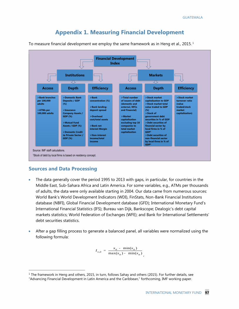
GUATEMALA
INTERNATIONAL MONETARY FUND 97
Appendix 1. Measuring Financial Development
To measure financial development we employ the same framework as in Heng et al., 2015. 1
Sources and Data Processing
The data generally cover the period 1995 to 2013 with gaps, in particular, for countries in the
Middle East, Sub-Sahara Africa and Latin America. For some variables, e.g., ATMs per thousands
of adults, the data were only available starting in 2004. Our data came from numerous sources:
World Bank’s World Development Indicators (WDI), FinStats, Non-Bank Financial Institutions
database (NBFI), Global Financial Development database (GFD); International Monetary Fund’s
International Financial Statistics (IFS); Bureau van Dijk, Bankscope; Dealogic’s debt capital
markets statistics; World Federation of Exchanges (WFE); and Bank for International Settlements’
debt securities statistics.
After a gap filling process to generate a balanced panel, all variables were normalized using the
following formula:
,
min( )
max( ) min( )
it itx it
it it
x xI
x x
-=
-,
1 The framework in Heng and others, 2015, in turn, follows Sahay and others (2015). For further details, see
“Advancing Financial Development in Latin America and the Caribbean,” forthcoming, IMF working paper.
Source: IMF staff calculations.
1Stock of debt by local firms is based on residency concept.
Financial Development
Index
Institutions Markets
Access EfficiencyDepth Access EfficiencyDepth
Bank branches
per 100,000
adults
ATMs per
100,000 adults
Domestic Bank
Deposits / GDP
(%)
Insurance
Company Assets /
GDP (%)
Mutual Fund
Assets / GDP (%)
Domestic Credit
to Private Sector /
GDP (%)
Bank
concentration (%)
Bank lending-
deposit spread
Overhead
cost/total assets
Bank net
interest Margin
Non-interest
income/total
income
Total number
of issuers of debt
(domestic and
external, NFCs
and Financial)
Market
capitalization
excluding top 10
companies to
total market
capitalization
Stock market
capitalization to GDP
Stock market total
value traded to GDP
(%)
Stock of
government debt
securities in % of GDP
Debt securities of
financial sector by
local firms in % of
GDP1
Debt securities of
non-financial sector
by local firms in % of
GDP1
Stock market
turnover ratio
(value
traded/stock
market
capitalization)

GUATEMALA
98 INTERNATIONAL MONETARY FUND
where ,x itI is the normalized variable x of country i on year t,
min( )itx is the lowest value of variable
itx over all i-t; and
max( )itx is the highest value of itx
. For variables capturing lack of financial
development, such as interest rate spread, bank asset concentration, overhead costs, net interest
margin, and non-interest income, one minus the formula above was used.
The weights were estimated with principal component analysis in levels and differences, factor
analysis in levels and differences, as well as equal weights within a subcomponent of the index. For
most of the methods the weights were not very different from equal weights and econometric
results were robust to the method of aggregation. For simplicity, we use an index with equal
weights.
Regression Frameworks
Regressions use 5-year averages in order to abstract from cyclical fluctuations, and estimated
using dynamic panel techniques common in the growth literature.
Financial Development Gaps
The benchmarking regressions link financial development (FD), institutions (FI) and markets (FM)
development indices to fundamentals. Following the literature on benchmarking financial
development (Beck and others 2008) fundamentals (FIitX
) included initial income per capita,
government consumption to GDP, inflation, trade openness, educational attainment proxied by
the average number of years of secondary schooling for people 25+, population growth, capital
account openness, the size of the shadow economy (given its importance for the LAC region)
and the rule of law. Instruments ( itZ) for financial development such as the rule of law and legal
origin dummies were also used. Predicted norms were computed using the following equation:
δ δ1 2' 'FI FI FIit it it t itFI h e= + + +X Z
,
where itFI stands for one of the financial indices (FD, FI or FM). Gaps shown are the difference
between the actual values of the index and the calculated norms.
Financial Development, Growth, and Stability
The link between financial development, growth and stability was examined using a dynamic
panel regression framework. Real GDP growth ( itYD) is linked to financial development allowing
for a potential non-linearity by adding a square of financial development while controlling for
other factors that are likely to affect growth (below). In the case of individual sub-components of
FI and FM, the interaction term between these two indices is included. The controls for the
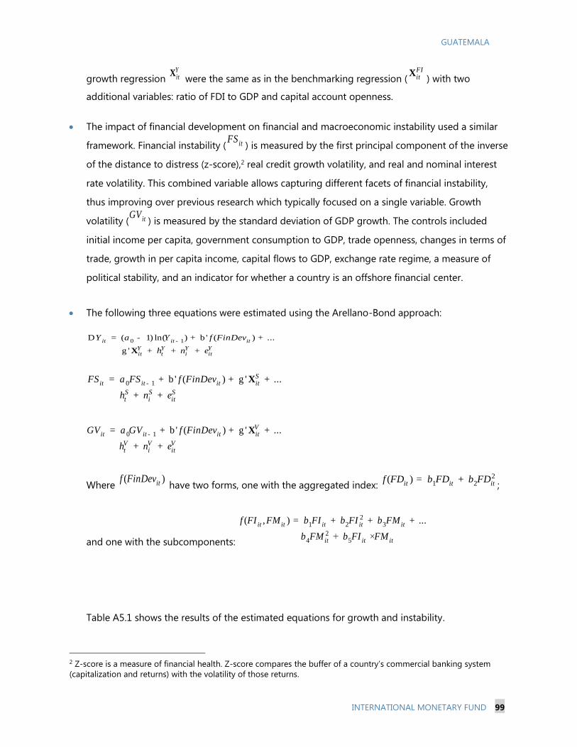
GUATEMALA
INTERNATIONAL MONETARY FUND 99
growth regression YitX
were the same as in the benchmarking regression (FIitX
) with two
additional variables: ratio of FDI to GDP and capital account openness.
The impact of financial development on financial and macroeconomic instability used a similar
framework. Financial instability ( itFS) is measured by the first principal component of the inverse
of the distance to distress (z-score),2 real credit growth volatility, and real and nominal interest
rate volatility. This combined variable allows capturing different facets of financial instability,
thus improving over previous research which typically focused on a single variable. Growth
volatility ( itGV) is measured by the standard deviation of GDP growth. The controls included
initial income per capita, government consumption to GDP, trade openness, changes in terms of
trade, growth in per capita income, capital flows to GDP, exchange rate regime, a measure of
political stability, and an indicator for whether a country is an offshore financial center.
The following three equations were estimated using the Arellano-Bond approach:
0 1( ' ( ) ...
'
1) ln( )it it it
Y Y Y Yit t i it
Y Y f FinDeva
h n e
-D = + b +
+ + +
-
g X
0 1 ' ( ) ' ...
Sit it
S S Sit
i
t
it
i
t f FinDevFS FSa
h n e
-= + b + g +
+ +
X
0 1 ' ( ) ' ...
Vit it it it
V V Vt i it
GV GV f FinDeva
h n e
-= + b + g +
+ +
X
Where ( )itf FinDev
have two forms, one with the aggregated index: 2
1 2( )it it itf FD FD FDb b= +;
and one with the subcomponents:
21 2 3
24 5
( , ) ...
it it it it it
it it it
f FI FM FI FI FM
FM FI FM
b b b
b b
= + + +
+ ×
Table A5.1 shows the results of the estimated equations for growth and instability.
2 Z-score is a measure of financial health. Z-score compares the buffer of a country’s commercial banking system
(capitalization and returns) with the volatility of those returns.
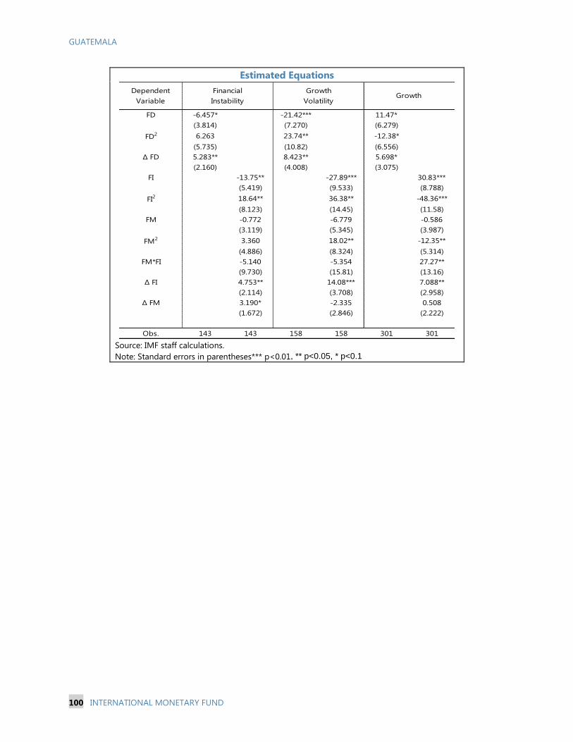
GUATEMALA
100 INTERNATIONAL MONETARY FUND
Estimated Equations
Source: IMF staff calculations.
Note: Standard errors in parentheses*** p<0.01, ** p<0.05, * p<0.1
Dependent
Variable
FD -6.457* -21.42*** 11.47*
(3.814) (7.270) (6.279)
FD2 6.263 23.74** -12.38*
(5.735) (10.82) (6.556)
Δ FD 5.283** 8.423** 5.698*
(2.160) (4.008) (3.075)
FI -13.75** -27.89*** 30.83***
(5.419) (9.533) (8.788)
FI2 18.64** 36.38** -48.36***
(8.123) (14.45) (11.58)
FM -0.772 -6.779 -0.586
(3.119) (5.345) (3.987)
FM2 3.360 18.02** -12.35**
(4.886) (8.324) (5.314)
FM*FI -5.140 -5.354 27.27**
(9.730) (15.81) (13.16)
Δ FI 4.753** 14.08*** 7.088**
(2.114) (3.708) (2.958)
Δ FM 3.190* -2.335 0.508
(1.672) (2.846) (2.222)
Obs. 143 143 158 158 301 301
Financial
Instability
Growth
VolatilityGrowth

GUATEMALA
INTERNATIONAL MONETARY FUND 101
Appendix 2. Construction of the Financial Inclusion Index This Appendix explains the construction of Indices of Financial Inclusion and its components and
provides an overview of the data and its processing for the construction of indices.
Measuring Financial Inclusion
Since there is no commonly accepted definition of financial inclusion we used a practical definition
for the purpose of this note, namely, access and effective usage of financial services by households
and firms. We employ multi-dimensional indices to capture different faucets of financial inclusion. In
particular, we construct three multi-dimensional indices capturing different angles of financial
inclusion: (i) usage of financial services by households (Findex); (ii) usage of financial services by
SMEs (Enterprise Survey); and (iii) access to financial institutions (Financial Access Survey). The
diagram below illustrates indicators included in each of the indices. We chose indicators that cover
the most important aspects of financial inclusion emphasized in the literature, while taking into
account data constraints. For example, the household inclusion index encompasses information on
the use of bank accounts, savings, borrowing, and payment methods but omits information on
insurance due to data constraints. We also chose not to combine the three indices into a single
index, notably because cross-country data coverage across households and firms varies
substantially. Instead, we compare Guatemala and other LAC countries to other regions and for
households across time,1 separately on each dimension.2
Financial Inclusion Index
1 Findex data is available for two years: 2011 and 2014. 2 We explore different aggregation methods, namely, weights derived from the principle component analysis
(Camara, N., and D. Tuesta, 2014), factor analysis (Amidžić et al., 2014) and equal weights. The results are similar
when using alternative measures (see Appendix 2). For simplicity of exposition we present the results for indices
constructed using equal weights.
GUATEMALA
102 INTERNATIONAL MONETARY FUND
Data Sources and Processing
Table below shows the main data sources. The data from Global Findex covers the period for 2011
and 2014 only. The data point from enterprise survey is the latest observation available.
From the components to the composite index
All variables were normalized using the following formula: Ix,it
𝐼𝑥,𝑖𝑡=𝑥𝑖𝑡−min (𝑥𝑖𝑡)
max(𝑥𝑖𝑡)−min (𝑥𝑖𝑡)
Where 𝐼𝑥,𝑖𝑡 is the normalized variable x of country i on year t, min (𝑥𝑖𝑡) is the lowest value of variable
𝑥𝑖𝑡 over all it; and max(𝑥𝑖𝑡) is the highest value of 𝑥𝑖𝑡. For those variables that capture a lack of
financial inclusion, such as Value of collateral needed for a loan and percent of firms identifying access
or cost of finance as major constraint, the reverse formula was used:
𝐼𝑥,𝑖𝑡=1 −𝑥𝑖𝑡−min (𝑥𝑖𝑡)
max(𝑥𝑖𝑡)−min (𝑥𝑖𝑡)
Several methods were used to estimate the weights: principal component analysis with the variables
in levels and in differences, factor analysis with the variables in levels and in differences, as well as
equal weights within a subcomponent of the index. For most of the methods the weights were not
very different from equal weights and econometric results were robust to the method of
aggregation. Thus, for simplicity of exposition the paper presents an index with equal weights.

GUATEMALA
INTERNATIONAL MONETARY FUND 103
Household Inclusion Index
Region 2011
East Asia and Pacific 9
Europe and Central Asia 29
Latin America 20
Middle East and North Africa 9
South Asia 6
Sub-Sahara Africa 31
Total 104
Region 2014
East Asia and Pacific 9
Europe and Central Asia 29
Latin America 20
Middle East and North Africa 9
South Asia 6
Sub-Sahara Africa 31
Total 104
Firm Inclusion Index
Region M.R.A. 1/
East Asia and Pacific 9
Europe and Central Asia 2
Latin America 31
Middle East and North Africa 5
South Asia 4
Sub-Sahara Africa 28
Total 79
Indicies Subcomponents Variables Sources
Account at a formal financial institution (% age 15+) Global Findex
ATM is main mode of withdrawal (% with an account, age
15+)
Global Findex
Debit card (% age 15+) Global Findex
Loan from a financial institution in the past year (% age 15+) Global Findex
Saved at a financial institution in the past year (% age 15+) Global Findex
% of SMEs Firms With a Checking or Savings Account Enterprise Survey
% of SME Firms With Bank Loans/line of Credit Enterprise Survey
% of SME Firms Using Banks to Finance Investments Enterprise Survey
Working Capital Bank Financing (%) Enterprise Survey
Value of Collateral Needed for a Loan (% of the Loan
Amount)
Enterprise Survey
% of SME Firms not needing a loan Enterprise Survey
% of SME Firms Identifying Access/cost of Finance as a
Major Constraint
Enterprise Survey
Number of ATMs per 1,000 sq km IMF, Financial Access Survey
Number of branches of ODCs per 1,000 sq km IMF, Financial Access Survey
Number of branches per 100,000 adults IMF, Financial Access Survey
Number of ATMs per 100,000 adults IMF, Financial Access Survey
Households
Firms/SMEs
(Enterprise Survey,
<100 employees)
Use of Financial Services
Access to financial infrastructure
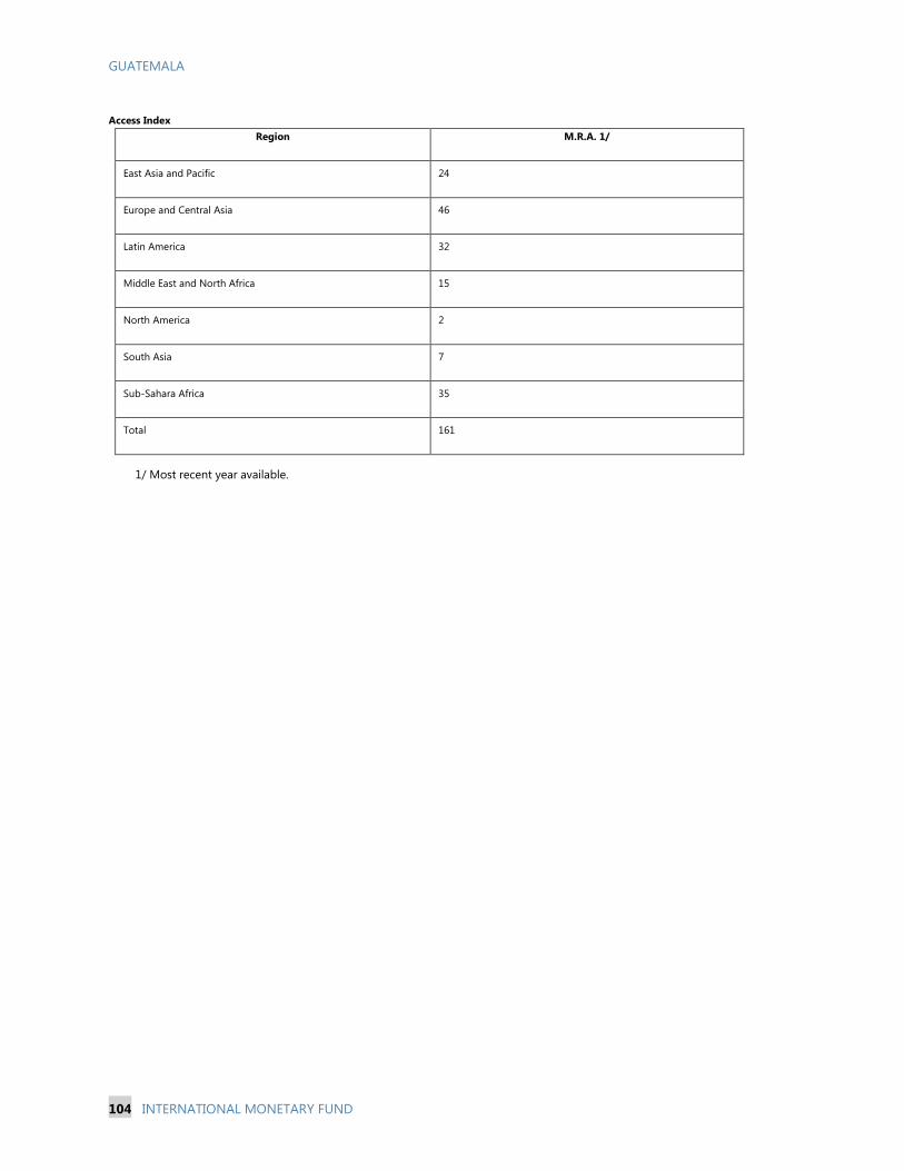
GUATEMALA
104 INTERNATIONAL MONETARY FUND
Access Index
Region M.R.A. 1/
East Asia and Pacific 24
Europe and Central Asia 46
Latin America 32
Middle East and North Africa 15
North America 2
South Asia 7
Sub-Sahara Africa 35
Total 161
1/ Most recent year available.
GUATEMALA
INTERNATIONAL MONETARY FUND 105
Appendix 3. Model Calibration
The model features an economy where agents differ in their talent and wealth. Each person has to
decide whether to become a worker (earn wages) or an entrepreneur (earn profits) and whether to
pay a fixed participation cost to be able to borrow from the banking system. Entrepreneurs then
decide on how much of their wealth to invest in their business, whether and how much to borrow at
the going interest rate, and how many workers to employ at the going wage rate. The output from
business projects depends on the amount of capital invested, the amount of labor hired, as well as
on the entrepreneur’s talent. In the model, the magnitude of the participation cost represents the
cost of financial contracting. The higher is this cost, the more agents remain in credit autarky.
Moreover, it tends to disproportionately exclude poor but talented individuals as the fixed cost
amounts to a larger fraction of their wealth.
Once in the banking system, the amount of credit available is constrained by other financial frictions. If
an entrepreneur has paid the participation cost, he or she can borrow from the banking system at the
going interest rate. The model assumes that a business can fail for external reasons (“bad luck”), with
some probability. Given imperfect enforceability of contracts, entrepreneurs have to post personal
wealth as collateral for the loan. Since banks runs the risk that entrepreneurs can defraud them, this
constrains the amount that can be borrowed. Therefore, weak contract enforceability leads to lower
leverage, imposing borrowing constraints on entrepreneurs. A second friction is modeled as arising
from asymmetric information between the bank and the borrower. The underlying intuition is that if the
entrepreneur does not pay back the loan, the bank cannot be sure whether the business actually failed.
Banks have to pay an audit or monitoring cost to find out. Otherwise, entrepreneurs could benefit from
claiming failure and keep the profits. These costs―measure of the degree of intermediation costs in the
economy―are recuperated by banks through interest rates and high overhead fees.1
In the baseline, the model is calibrated to data for 12 LAC countries. Firm-level data for 2005 from the
World Bank Enterprise Survey are used, in addition to standard macroeconomic and financial variables
(savings rate, non-performing loans (NPLs), and interest rate spreads) for 2010 or the latest year
available. While lack of financial inclusion is an even more acute problem for firms in the informal
sector, the model focuses primarily on formal sector firms. The model’s key parameters are jointly
chosen to match the simulated moments, such as the percent of firms with credit and the firm
employment distribution, with the actual data for each country (see Dabla-Norris et al., 2015, for
details).
1 In the model, the bank’s optimal verification strategy follows Townsend (1979), whereby verification only occurs if
the entrepreneur cannot pay the face value of the loan. This happens when the entrepreneur is highly leveraged and
also faces a production failure. As a result, banks only monitor if a production failure is reported and the loan
contract is highly-leveraged. A low-leveraged loan implies that entrepreneurs are not borrowing much from the bank
and therefore the required repayment is small.