GUIDANCE MANUAL FOR ENVIRONMENTAL SITE

CHARACTERIZATION IN SUPPORT OF HUMAN HEALTH RISK ASSESSMENT

VOLUME 1 TECHNICAL GUIDANCE

July 2008

FINAL DRAFT

Prepared by:

Contaminated Sites Division

Safe Environments Programme

Our mission is to help the people of Canada maintain and improve their health. Health Canada

April 2008 - i -

Final

PREFACE

This guidance document was prepared in support of the Federal Contaminated Sites Action Plan (FCSAP), a program designed to ensure improved and continuing federal environmental stewardship as it relates to contaminated sites located on federally owned or operated properties. As is common with national guidance, this document will not satisfy all of the requirements presented by contaminated site risk assessment in every case.

Guidance for Environmental Site Characterization in Support of Human Health Risk Assessment (Volumes 1-3) was prepared by Golder Associates Ltd. for the Contaminated Sites Division, Safe Environments Programme, Health Canada. A draft version of this guidance was circulated widely to internal (federal government) and external (CCME and others) stakeholders to make the document as complete and defensible as possible, within the limitations presented by the federal contaminated sites program and Health Canada commitments, policies, and obligations with respect to health risk assessment and protection.

It is anticipated that revisions to this document will be necessary from time to time to reflect new technology and practices as the field of environmental site characterization advances. Health Canada should be consulted at the address below to confirm that the version of the document in your possession is the most recent edition and that the most recent guidance is considered.

Methods and any reference to specific sampling equipment provided in this guidance is provided for information purposes only. Health Canada does not warrant the use of any of these methods or equipment. The responsibility for selection and use lies solely with the user.

Questions, comments, criticisms, suggested additions or revisions to this document should be directed to:

Contaminated Sites Division Safe Environments Programme Health Canada 269 Laurier Avenue W, 4th Floor - Mail Stop: 4905A Ottawa, Ontario K1A 0K9 Fax: (613) 952-8857 E-mail: cs-sc@hc-sc.gc.ca See also: http://www.hc-sc.gc.ca/hecs-sesc/ehas/contaminated_sites.htm

April 2008 - ii -

Final

ACKNOWLEDGEMENTS

The primary authors of this guidance were Dr. Ian Hers, Mr. Guy Patrick, and Dr. Reidar Zapf-Gilje of Golder Associates Ltd. under contract to Health Canada. We truly appreciate the time commitment made by several organizations to review this guidance and provide valuable comment. Thank you to Fisheries and Oceans Canada; Water Standards Section, Standards Development Branch, Ontario Ministry of the Environment; Groundwater Assessment and Remediation Section, Water Science & Technology Directorate, Environment Canada; ALS Laboratory Group; and, Air Toxics Ltd.

April 2008 - iii -

Final

TABLE OF CONTENTS

SECTION PAGE

1.0 INTRODUCTION......................................................................................... 1 1.1 Background and Purpose ........................................................................1 1.2 Intended Audience and Guidance Application.........................................1 1.3 Scope ......................................................................................................1 1.4 Guidance Outline.....................................................................................2

2.0 CONTAMINATED SITE INVESTIGATION AND MANAGEMENT PROCESS................................................................................................... 5 2.1 Integrated Risk Management Process for Contaminated Sites...............5 2.2 Site Characterization Process .................................................................5

2.2.1 Phased Investigation Approach ...................................................6 2.2.2 Data Quality as a Central Theme to the Site Characterization

Process........................................................................................6 2.3 Development of a Conceptual Site Model ...............................................7 2.4 Define the Project Background and Goals ............................................12 2.5 Establish the Investigation Objectives ...................................................13 2.6 Prepare a Sampling and Analysis Plan .................................................13

2.6.1 Review of Existing Data.............................................................14 2.6.2 Pre-mobilization Tasks ..............................................................14 2.6.3 Sampling Media, Data Types and Investigation Tools...............14 2.6.4 Sampling Rationale and Design ................................................16 2.6.5 Sampling and Analysis Methods and Quality Assurance Project

Plan............................................................................................18 2.7 Conduct the Field Investigation Program – Conventional Phased Approach and Expedited Site Assessment Process .........................................19 2.8 Validate and Interpret Data....................................................................21 2.9 Resources and Weblinks.......................................................................22 2.10 References ............................................................................................23

3.0 QUALITY ASSURANCE/QUALITY CONTROL........................................ 25 3.1 Quality Assurance Project Plan .............................................................25 3.2 Data Quality Indicators ..........................................................................27 3.3 Quality Control.......................................................................................28

3.3.1 Quality Control Checks and Samples ........................................28 3.3.2 Recommended Minimum Frequency of Quality Control Samples29

3.4 Data Quality Targets..............................................................................30 3.4.1 Duplicate Samples.....................................................................31

3.5 Reporting of QA/QC ..............................................................................31 3.6 References ............................................................................................32

April 2008 - iv -

Final

4.0 CONCEPTUAL SITE MODEL FOR CONTAMINATED SITES................ 34 4.1 Contamination Sources and Types .......................................................34

4.1.1 Overview....................................................................................34 4.1.2 Common Types of Contamination .............................................35 4.1.3 Non-Point Sources of Contamination ........................................36 4.1.4 Emergent or Less Common Chemicals .....................................39

4.2 LNAPL and DNAPL ...............................................................................40 4.3 Groundwater Pathway ...........................................................................41

4.3.1 Partitioning.................................................................................42 4.3.2 Unsaturated Zone Chemical Transport......................................43 4.3.3 Groundwater Contaminant Transport ........................................44 4.3.4 Considerations for Fractured Bedrock .......................................46 4.3.5 Considerations for Permafrost ...................................................47

4.4 Soil Vapour Intrusion Pathway ..............................................................48 4.4.1 Contamination Sources .............................................................49 4.4.2 Chemical Transfer to Vapour Phase (Volatilization) ..................50 4.4.3 Vadose Zone Fate and Transport Processes ............................52 4.4.4 Near-Building Processes for Soil Vapour Intrusion....................54 4.4.5 Summary ...................................................................................55 4.4.6 Resources, References and Links.............................................55

4.5 References ............................................................................................63 5.0 SOIL CHARACTERIZATION GUIDANCE................................................ 68

5.1 Context, Purpose and Scope.................................................................68 5.2 Conceptual Site Model for Soil Characterization ...................................69 5.3 Soil Sampling Design Considerations ...................................................70

5.3.1 Sampling Design Objectives......................................................70 5.3.2 Representative Sampling Challenges........................................72 5.3.3 Sampling Designs......................................................................72 5.3.4 Statistical Methods.....................................................................76 5.3.5 Discrete and Composite Samples .............................................80

5.4 Selection of Sampling Design for Soil Investigation ..............................81 5.4.1 Preliminary Investigation Sampling............................................81 5.4.2 Detailed Investigation Sampling ................................................82

5.5 Investigation Soil Sampling Methods.....................................................83 5.6 Field Analytical Methods........................................................................86

5.6.1 Headspace Vapour Tests ..........................................................87 5.6.2 Colourimetric Tests....................................................................88 5.6.3 Immunoassay Tests...................................................................89 5.6.4 X-ray fluorescence (XRF) ..........................................................90

5.7 Field Preservation of Soil Samples for VOC Analysis ...........................91 5.8 Data Validation and Interpretation .........................................................92

5.8.1 Evaluation of Data Distributions.................................................92 5.8.2 Non-Detect Values.....................................................................93

April 2008 - v -

Final

5.8.3 Statistical Characterization of Soil Data.....................................94 5.8.4 Comparison of Population Means..............................................95 5.8.5 Data Presentation and Reporting ..............................................96

5.9 Resources and Weblinks.......................................................................96 5.10 REFERENCES ......................................................................................99

5.10.1 Sampling Design - Confirmation of Remediation.....................102 5.10.2 Sampling Design - Ex situ (Stockpile) Characterization ..........103

6.0 GROUNDWATER CHARACTERIZATION GUIDANCE......................... 104 6.1 Purpose, Background and Need .........................................................105

6.1.1 Obtaining Representative Samples from the Well ...................106 6.1.2 Non-Aqueous Phase Liquids (NAPLs).....................................110

6.2 Conceptual Site Models For Groundwater Characterization ...............111 6.3 Approach and Sampling Design ..........................................................112

6.3.1 Intrusive Field Program For Groundwater Characterization ....112 6.3.2 Addressing the Issue of Scale .................................................113 6.3.3 Acquiring Groundwater Quality Information.............................115 6.3.4 Available Technologies............................................................115 6.3.5 Direct-Push Technologies for Groundwater Characterization .118

6.4 Acquiring Hydrogeologic Information...................................................121 6.4.1 Groundwater Flow Direction ....................................................121 6.4.2 Groundwater Velocity ..............................................................122

6.5 Monitoring and Monitoring Networks ...................................................124 6.5.1 Well Screen Length and Well Completion Intervals.................124 6.5.2 Horizontal Spacing of Data Points ...........................................127 6.5.3 Vertical Spacing of Data Points ...............................................129

6.6 Field and Laboratory Data Acquisition.................................................131 6.6.1 Well Development....................................................................131 6.6.2 Well Purging and Sampling .....................................................132 6.6.3 Field Laboratories ....................................................................135 6.6.4 Special Considerations ............................................................135 6.6.5 Selection of Analytical Tests....................................................136 6.6.6 Data Validation and Quality Assurance/Quality Control ..........137

6.7 Well Abandonment ..............................................................................138 6.8 Data Assessment and Interpretation ...................................................138

6.8.1 Conceptual Site Model Development ......................................138 6.8.2 Data Presentation and Reporting ............................................139 6.8.3 Modeling Issues.......................................................................140

6.9 References ..........................................................................................141 7.0 SOIL VAPOUR GUIDANCE.................................................................... 143

7.1 Context, Purpose and Scope...............................................................143 7.2 Conceptual Site Model for Soil Vapour Characterization ....................144 7.3 Study Objectives..................................................................................144 7.4 Soil Vapour Sampling Approach and Design ......................................145

April 2008 - vi -

Final

7.4.1 Overview of Sampling Strategy ...............................................145 7.4.2 Sampling Locations .................................................................146 7.4.3 When to Sample and Sampling Frequency .............................154 7.4.4 Biodegradation Assessment ....................................................155

7.5 Soil Gas Probe Construction and Installation ......................................157 7.5.1 Probes Installed in Boreholes ..................................................157 7.5.2 Probes Installed Using Direct Push Technology......................159 7.5.3 Driven Probes ..........................................................................159 7.5.4 Use of Water Table Monitoring Wells as Soil Gas Probes ......160 7.5.5 Subslab Soil Gas Probes.........................................................160 7.5.6 Probe Materials........................................................................161 7.5.7 Short-Circuiting Considerations ...............................................162

7.6 Soil Gas Sampling Procedures............................................................162 7.6.1 Probe Development and Soil Gas Equilibration.......................162 7.6.2 Flow and Vacuum (Probe Performance) Check ......................163 7.6.3 Sampling Container or Device .................................................163 7.6.4 Decontamination of Sampling Equipment................................165 7.6.5 Testing of Equipment for Leaks and Short Circuiting ..............165 7.6.6 Sample Probe Purging and Sampling......................................166

7.7 Soil Gas Analysis.................................................................................168 7.7.1 Selection of Method .................................................................168 7.7.2 Field Detectors.........................................................................168 7.7.3 Field Laboratory Analysis ........................................................171 7.7.4 Fixed Laboratory Analysis .......................................................171 7.7.5 Quality Assurance / Quality Control Considerations................176

7.8 Soil and Groundwater Characterization...............................................178 7.8.1 Groundwater Data ...................................................................179 7.8.2 Soil Data ..................................................................................180

7.9 Ancillary Data ......................................................................................180 7.10 Data Interpretation and Analysis .........................................................182

7.10.1 Data Organization and Reporting ............................................182 7.10.2 Data Quality Analysis...............................................................183 7.10.3 Data Consistency Analysis ......................................................184 7.10.4 Further Evaluation ...................................................................184

7.11 Resources and Weblinks.....................................................................185 7.12 References ..........................................................................................185

8.0 INDOOR AIR QUALITY TESTING FOR EVALUATION OF SOIL VAPOUR INTRUSION............................................................................................. 194 8.1 Context, Purpose and Scope...............................................................194 8.2 Conceptual Site Model for Indoor Air...................................................195

8.2.1 Background Indoor Air Concentrations....................................196 8.2.2 Building Foundation Construction............................................198 8.2.3 Building Ventilation ..................................................................198

April 2008 - vii -

Final

8.2.4 Building Depressurization and Weather Conditions ................199 8.2.5 Mixing of Vapours Inside Building............................................200 8.2.6 Vapour Depletion Mechanisms................................................200

8.3 Development of Indoor Air Quality Study Approach and Design.........201 8.3.1 Define Study Objectives ..........................................................201 8.3.2 Identify Target Compounds .....................................................201 8.3.3 Develop Communications Program .........................................202 8.3.4 Conduct Pre-Sampling Building Survey...................................202 8.3.5 Conduct Preliminary Screening ...............................................202 8.3.6 Identify Immediate Health or Safety Concerns ........................203 8.3.7 Define Number and Locations of Indoor and Outdoor Air Samples ........................................................203 8.3.8 Define Sampling Duration........................................................204 8.3.9 Define Sampling Frequency.....................................................204 8.3.10 Preparing the Building for Sampling and Conditions During

Sampling..................................................................................205 8.4 Indoor Air Analytical Methods..............................................................206

8.4.1 Issues for Air Analysis Using USEPA Method TO-15..............207 8.4.2 Issues for Air Analysis using Passive Diffusive Badge Samplers .......................................................208

8.5 Data Interpretation and Analysis .........................................................210 8.5.1 Data Organization and Reporting ............................................210 8.5.2 Data Quality Evaluation ...........................................................210 8.5.3 Methods for Discerning Contributions of Background from Indoor Sources ............................................210

8.6 Resources and Weblinks.....................................................................213 8.7 References ..........................................................................................214

9.0 ACRONYMS ........................................................................................... 218

April 2008 - viii -

Final

LIST OF TABLES Table 2-1 Conceptual Site Model Component Checklist Table 2-2 Potential Data Requirements for Exposure Pathway Modeling Table 2-3 Spatial and Temporal Variability between Different Media Table 3-1 Components of a Quality Assurance Project Plan Table 3-2 Description of Primary Data Quality Indicators Table 4-1 Contaminants Commonly Associated with Various Industrial and

Governmental Operations and Activities (adapted from Health Canada PQRA, 2004).

Table 5-1 Description of Common Soil Sampling Methods Table 5-2 Stockpile Characterization Guidance Table 6-1 Types of Groundwater Quality Information Table 7-1 Comparison of Soil Vapour Measurement Locations Table 7-2 Evaluation of Factors Affecting Below Building Hydrocarbon Vapour

Bioattenuation and Soil Vapour Data Representativeness Table 7-3 Soil Gas Sample Collection Containers and Devices Table 7-4 Summary of Common Soil Vapour Sampling and Analysis Methods Table 8-1 Dominant Sources of VOCs in Residential Indoor Air Table 8-2 Compilation of Indoor Air Quality Data from Canadian Studies LIST OF FIGURES Figure 1-1 Site Characterization Process and Guidance Outline Figure 2-1 Integrated Risk Management Process Figure 2-2 Conceptual Site Model – Risk Focus Figure 2-3 Conceptual Site Model – Hydrogeological Focus Figure 2-4 Conceptual Exposure Model for Residential Scenario Figure 4-1 Groundwater Pathway Conceptual Model Figure 4-2 Conceptual Water Balance Model Figure 4-3 Distribution of Continuous and Discontinuous Permafrost in Canada Figure 4-4 Example of a Conceptual Site Model for Vapour Intrusion Figure 4-5 Fresh Water Lens Figure 4-6 Interface Plume Development Figure 4-7 Falling Water Table Figure 4-8 Lateral Diffusion and Preferential Pathways Figure 4-9 Conceptual Model for Aerobic Biodegradation Figure 4-10 Stack and Wind Effect on Depressurisation (NPL=neutral pressure line) Figure 5-1 Process for Defining Study Boundaries Figure 5-2 Some Common Two-Dimensional Sampling Designs Figure 5-3 Required Sample Grid Spacing Corresponding to Acceptable Probability

(β) of Not Finding Contamination Hot-spot. Figure 6-1 A. Pumping Well and Monitoring Well Completed in Multi-layered

Aquifer. B. Varying Concentrations in Multi-layered system. Figure 6-2 LNAPL Conceptual Model Figure 6-3 A. Plan Showing Elevation Contours of Potentiometric Surface Across a

Site. B and C. Plan Showing Contours of cis-1,2-dichloroethene in Groundwater. Note that both drawings are based on the same data set.

April 2008 - ix -

Final

Figure 7-1 Results of 3-D Oxygen-Limited Soil Vapour Transport Modeling for High Concentration Source (Cg=100 mg/L) and Moderate Concentration Source (Cg=20 mg/L) (from Abreu and Johnson, 2005)

Figure 7-2 Soil Vapour Sampling Locations and Vertical Profile Concept Figure 7-3 Lateral Transect Concept Figure 7-4 USEPA (2004) Recommended Design for Subslab Soil Gas Probes Figure 8-1 Framework for IAQ Sampling and Analysis Program LIST OF APPENDICES Appendix 5-1 Confirmation of Remediation Sampling Appendix 7-1 Selected Laboratory Analytical Methods

April 2008 - 1 -

Final

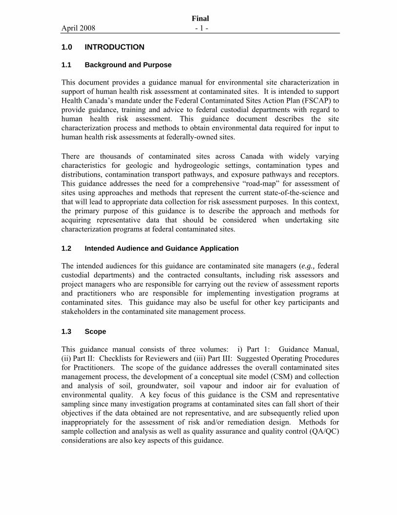
1.0 INTRODUCTION

1.1 Background and Purpose

This document provides a guidance manual for environmental site characterization in support of human health risk assessment at contaminated sites. It is intended to support Health Canada’s mandate under the Federal Contaminated Sites Action Plan (FSCAP) to provide guidance, training and advice to federal custodial departments with regard to human health risk assessment. This guidance document describes the site characterization process and methods to obtain environmental data required for input to human health risk assessments at federally-owned sites.

There are thousands of contaminated sites across Canada with widely varying characteristics for geologic and hydrogeologic settings, contamination types and distributions, contamination transport pathways, and exposure pathways and receptors. This guidance addresses the need for a comprehensive “road-map” for assessment of sites using approaches and methods that represent the current state-of-the-science and that will lead to appropriate data collection for risk assessment purposes. In this context, the primary purpose of this guidance is to describe the approach and methods for acquiring representative data that should be considered when undertaking site characterization programs at federal contaminated sites.

1.2 Intended Audience and Guidance Application

The intended audiences for this guidance are contaminated site managers (e.g., federal custodial departments) and the contracted consultants, including risk assessors and project managers who are responsible for carrying out the review of assessment reports and practitioners who are responsible for implementing investigation programs at contaminated sites. This guidance may also be useful for other key participants and stakeholders in the contaminated site management process.

1.3 Scope

This guidance manual consists of three volumes: i) Part 1: Guidance Manual, (ii) Part II: Checklists for Reviewers and (iii) Part III: Suggested Operating Procedures for Practitioners. The scope of the guidance addresses the overall contaminated sites management process, the development of a conceptual site model (CSM) and collection and analysis of soil, groundwater, soil vapour and indoor air for evaluation of environmental quality. A key focus of this guidance is the CSM and representative sampling since many investigation programs at contaminated sites can fall short of their objectives if the data obtained are not representative, and are subsequently relied upon inappropriately for the assessment of risk and/or remediation design. Methods for sample collection and analysis as well as quality assurance and quality control (QA/QC) considerations are also key aspects of this guidance.

April 2008 - 2 -

Final

The guidance is, by intent, prescriptive in identifying minimum requirements or specific methods on key issues that warrant prescription; however, alternate methods may be acceptable where there is a supporting rationale for such methods. On issues where there is no clear consensus on methods or where different approaches may yield acceptable results, the guidance describes factors that should be considered when designing a environmental site characterization program.

While the focus of the guidance is to provide improve the quality of data used to support human health risk assessment, it provides approaches and methods that are highly relevant and useful in the contaminated site assessment process. The sampling and analysis of media that are less commonly required to assess human health risk (e.g., sediment and surface water) are not included in this guidance, but may be addressed in future modules of this guidance. Health Canada has concurrently developed guidance for biota, “Supplemental Guidance on Human Health Risk Assessment for Country Foods (HHRAFOODS)” (internal draft, April 2007). It is recommended that HHRAFOODS be consulted in conjunction with this guidance when consumption of contaminated biota is a potential exposure pathway.

This guidance is based on the knowledge and experience of the authors and peer reviewers, as well as much of the latest available technical data and information. Nevertheless, this guidance is not intended to represent the definitive resource for application at all sites or situations, nor can it address all questions and issues that may arise during the contaminated site assessment process. New developments are expected in the future that could require updating of this guidance.

The guidance document includes a listing of selected tools, software and other resources, which may be found at the end of most chapters for reference purposes. For software, the focus has been on identifying programs that are free or low-cost. The identification of specific software and other tools should not be construed as an endorsement by Health Canada; the determination of the usefulness and applicability of these tools is the responsibility of the user.

1.4 Guidance Outline

Following this chapter, the guidance is divided into seven subject areas:

Chapter 2 Contaminated Sites Management and Investigation Process. This chapter presents an overview of the steps to successfully investigate a site; these comprise the development of a conceptual site model (CSM), defining the project background, goals and investigation objectives, the preparation of a sampling plan, and validation and interpretation of data.

Chapter 3 Quality Assurance / Quality Control. This chapter describes the key elements of a quality assurance / quality control (QA/QC) plan, and data quality indicators and checks that should be assessed as part of a contaminated site investigation program.

April 2008 - 3 -

Final

Chapter 4 Conceptual Site Model for Contaminated Sites. This chapter provides the background needed for the design of investigation programs and interpretation of data, and describes the key elements of the contaminated sites conceptual site model, contamination sources and types, and fate and transport processes.

Chapter 5 Soil Characterization Guidance. This chapter describes the process and considerations for collection of representative and valid data for characterization of soil quality. Sampling design and statistical considerations, sampling methods and field analytical methods are discussed.

Chapter 6 Groundwater Characterization Guidance. This chapter describes the process and considerations for obtaining representative groundwater quality data. The issues for groundwater quality assessments, recommended approach and methods, and supporting data and analysis needed for groundwater characterization are discussed.

Chapter 7 Soil Vapour Characterization Guidance. This chapter describes the soil vapour investigation approach and design process, soil vapour probe installation and sampling, soil vapour analysis, and data interpretation.

Chapter 8 Indoor Air Characterization Guidance. This chapter describes the process for indoor air testing, including preparatory steps, sampling design and methods, analytical considerations, and ancillary data that may be useful when evaluating soil vapour intrusion.

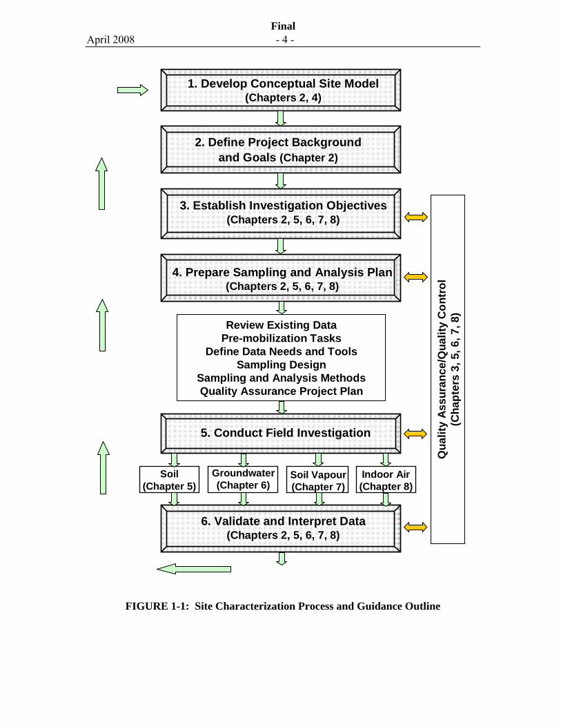
The site characterization process and guidance document outline is provided in Figure 1-1.

Part II of this guidance consists of checklists for reviewers evaluating contaminated site reports.

Part III of this guidance provides Suggested Operating Procedures (SOPs) for selected aspects of the site investigation process, as follows:

• SOP #1: Borehole Drilling and Installation of Monitoring Wells (in overburden).

• SOP #2: Soil Sampling.

• SOP #3: Low-Flow Groundwater Sampling.

• SOP #4: Soil Gas Probe Installation.

• SOP #5: Soil Gas Sampling.

• SOP #6: Soil Gas Probe Leak Tests.

April 2008 - 4 -

Final

FIGURE 1-1: Site Characterization Process and Guidance Outline

1. Develop Conceptual Site Model (Chapters 2, 4)

Soil(Chapter 5)

2. Define Project Backgroundand Goals (Chapter 2)

3. Establish Investigation Objectives(Chapters 2, 5, 6, 7, 8)

4. Prepare Sampling and Analysis Plan(Chapters 2, 5, 6, 7, 8)

Review Existing DataPre-mobilization Tasks

Define Data Needs and ToolsSampling Design

Sampling and Analysis MethodsQuality Assurance Project Plan

5. Conduct Field Investigation

6. Validate and Interpret Data(Chapters 2, 5, 6, 7, 8)

Qua

lity

Ass

uran

ce/Q

ualit

y C

ontr

ol(C

hapt

ers

3, 5

, 6, 7

, 8)

Groundwater (Chapter 6)

Soil Vapour (Chapter 7)

Indoor Air (Chapter 8)

April 2008 - 5 -

Final

2.0 CONTAMINATED SITE INVESTIGATION AND MANAGEMENT PROCESS

2.1 Integrated Risk Management Process for Contaminated Sites

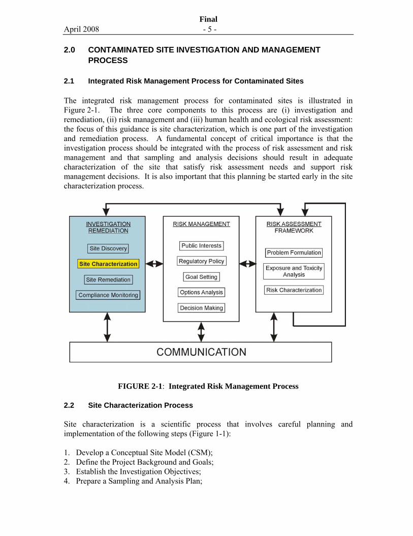
The integrated risk management process for contaminated sites is illustrated in Figure 2-1. The three core components to this process are (i) investigation and remediation, (ii) risk management and (iii) human health and ecological risk assessment: the focus of this guidance is site characterization, which is one part of the investigation and remediation process. A fundamental concept of critical importance is that the investigation process should be integrated with the process of risk assessment and risk management and that sampling and analysis decisions should result in adequate characterization of the site that satisfy risk assessment needs and support risk management decisions. It is also important that this planning be started early in the site characterization process.

FIGURE 2-1: Integrated Risk Management Process

2.2 Site Characterization Process

Site characterization is a scientific process that involves careful planning and implementation of the following steps (Figure 1-1):

1. Develop a Conceptual Site Model (CSM); 2. Define the Project Background and Goals; 3. Establish the Investigation Objectives; 4. Prepare a Sampling and Analysis Plan;

April 2008 - 6 -

Final

5. Conduct the Field Investigation Program; and, 6. Validate and Interpret the Data.

The site characterization process can be viewed as a scientific hypothesis, based on historical and current land use, that is continually updated and modified as new information is obtained. The above elements should be incorporated in a written proposal and/or project work plan. The steps are described in Sections 2.3 to 2.8.

2.2.1 Phased Investigation Approach

The site characterization process is often implemented in phases. Different terminology is used to describe these phases, but more important are the underlying concepts. The first phase, often referred to as a Phase I Environmental Site Assessment (ESA) or Preliminary Site Investigation (PSI), involves an evaluation of historical and current land use, a site reconnaissance and other information gathering techniques to assess the potential for site contamination. Typically, a Phase I ESA does not include a sampling and analysis component. The outcome of the Phase I ESA should be the identification of areas of potential environmental concern (APECs) and associated contaminants of potential concern (COPCs). Guidance on performing Phase I ESAs is provided in ASTM (2005) and CSA (2001).

Subsequent intrusive phases of investigation are often referred to as a Phase II ESA, designed to investigate whether contamination is present or absent (e.g., rule out the presence of elevated COPCs in relevant media), and a Phase III ESA, designed to delineate contamination and provide information required for risk assessment and remediation planning. Guidance on performing Phase II ESAs is provided in ASTM (2002) and CSA (2000).

2.2.2 Data Quality as a Central Theme to the Site Characterization Process

Fundamental to the site characterization process is data quality that enables goals and objectives for site characterization to be met. Data quality should be viewed in the broadest sense in that it is influenced by all facets of the site characterization process, ranging from the initial development of a conceptual site model and identification of goals and objectives, to more detailed planning phases of the project involving sampling design and determination of appropriate methods. This broad planning is sometimes referred to as the “data quality objective process”, which describes the overall planning process for contaminated site investigation in the context of activities that lead to acceptable data quality (USEPA, 2006).

More specifically, data quality can be viewed as the composite features or characteristics that bear upon the ability to fulfill project goals and objectives based on the intended use of the data. Data quality is much more than analytical accuracy or precision and involves all aspects of the site characterization process, including selection of sample locations, numbers of samples, when to sample, sampling methods, analytical parameters, sample handling, and analytical methods. A key concept is that the goal of

April 2008 - 7 -

Final

the investigation should be to obtain representative data that enables informed decisions to be made. The collection of non-representative samples will produce misleading or meaningless data, even if the analytical quality for those samples was near-perfect.

Obtaining representative data is closely linked to the sampling design, which involves consideration of the scale and frequency at which samples are analyzed. It is important that uncertainty be controlled to tolerable limits through a sampling design compatible with the goals of the risk assessment. The sources of uncertainty in data should be understood, and effectively communicated to the risk assessor. The importance of representative sampling is emphasized throughout this guidance given the inherent variability in site conditions that exists at contaminated sites.

2.3 Development of a Conceptual Site Model

The following discussion in an overview of the development of a conceptual site model. A more detailed in–depth discussion ins provided in Chapter 4.

The first step of the site characterization process is the development of a conceptual site model (CSM). A CSM is a visual representation and narrative description of the physical, chemical, and biological processes occurring, or that have occurred, at a site. The CSM should be able to tell the story of how the site became contaminated, how the contamination was and is transported, where the contamination will ultimately end up, and whom it may affect. A well-developed CSM provides decision makers with an effective tool that helps to organize, communicate, and interpret existing data, while also identifying areas where additional data are required. The CSM should be considered dynamic in nature and continuously updated and shared as new information becomes available (USEPA, 2002a; USEPA, 1996).

A CSM should provide information on the sources, types and extent of the contamination, it’s release and transport mechanisms, possible subsurface migration pathways, as well as potential receptors and the routes of exposure. As warranted, information on the current and future land use and community concerns should be incorporated into the CSM. The specific elements of the CSM may include:

• An overview of historical, current, and planned future land uses;

• A detailed description of the site and its physical setting that is used to form hypotheses about the release and ultimate fate of contamination at the site;

• Sources of contamination at the site, the potential chemicals of concern, and the media (soil, groundwater, surface water, sediments, soil vapour, indoor and outdoor air, country foods) that may be affected;

• The distribution of chemicals within each medium including information on the concentration, mass and/or flux;

April 2008 - 8 -

Final

• How contaminants may be migrating from the source(s), the media and pathways through which migration and exposure of potential human or ecological receptors could occur, and information needed to interpret contaminant migration such as geology, hydrogeology, hydrology and possible preferential pathways;

• Information on climate and meteorological conditions that may influence contamination distribution and migration;

• Where relevant, information pertinent to soil vapour intrusion into buildings including construction features of buildings (e.g., size, age, foundation depth and type, presence of foundation cracks, entry points for utilities), building heating, ventilation and air conditioning (HVAC) design and operation, and subsurface utility corridors; and,

• Information on human and ecological receptors and activity patterns at the site or at areas impacted by the site.

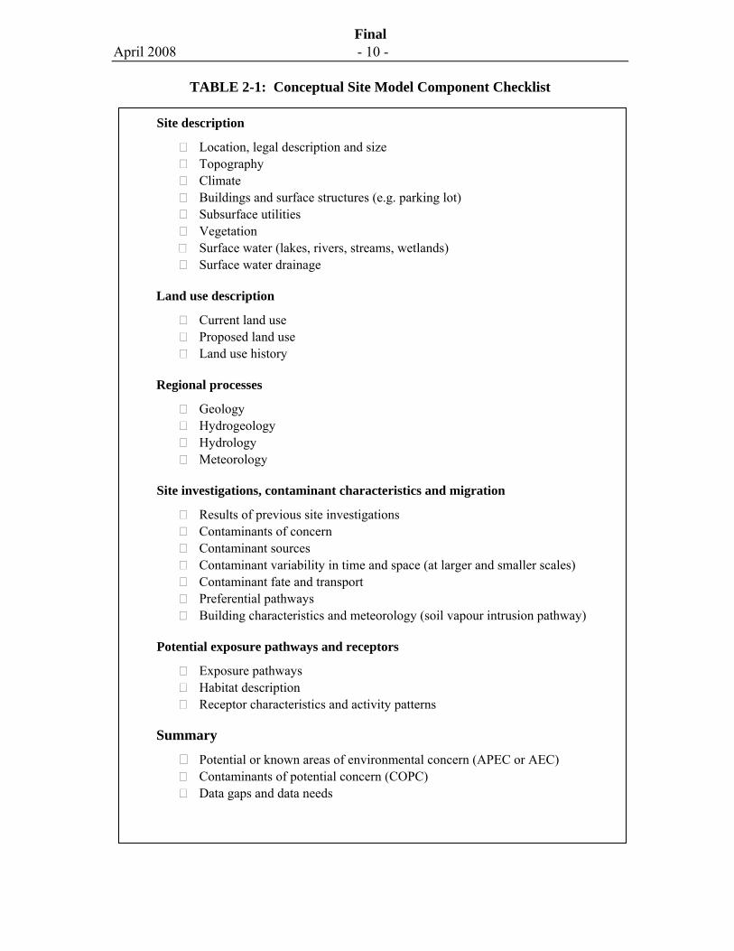
An overview checklist of the components of the conceptual site model is provided in Table 2-1. The CSM for contaminated sites is further described in Section 4.0 and additional details relevant to different media being sampled are provided in subsequent chapters.

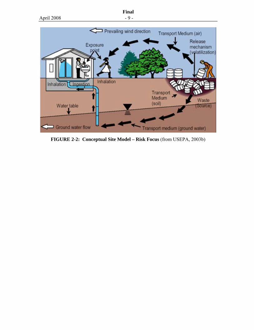
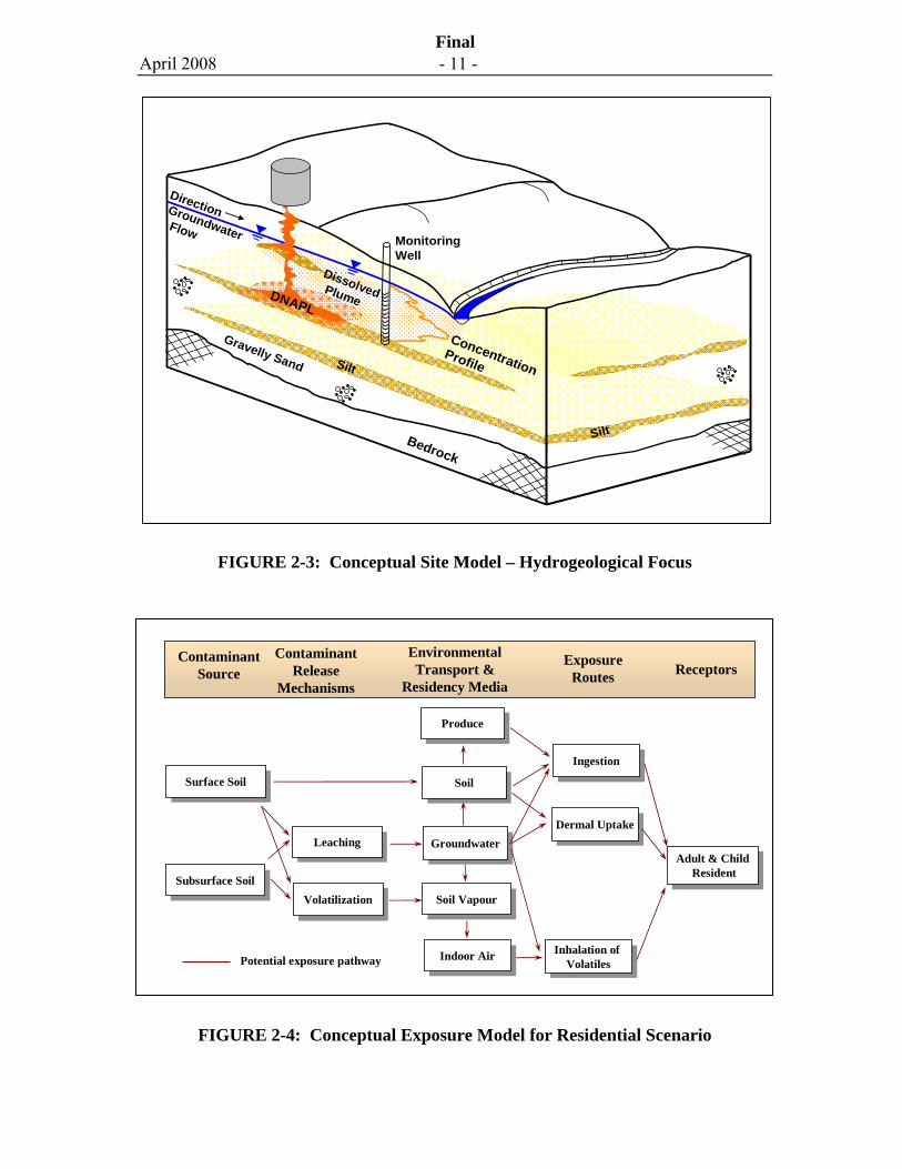
For the development of the CSM, it is helpful to prepare plans and cross sections (two-dimensional), and to at least conceptually, consider the three-dimensional contaminant distribution at a site. An example of a risk-focused CSM is shown in Figure 2-2 while a hydrogeological-focused CSM is shown in Figure 2-3. The CSM should show sufficient details and when possible, be drawn to scale, to realistically portray the characteristics of the site (see examples in Chapter 6).

A CSM is different than a conceptual exposure model (CEM) (Figure 2-4), which can also be developed in an effort to delineate exposure pathways from source to receptor in a risk assessment.

April 2008 - 9 -

Final

FIGURE 2-2: Conceptual Site Model – Risk Focus (from USEPA, 2003b)

April 2008 - 10 -

Final

TABLE 2-1: Conceptual Site Model Component Checklist

Site description

Location, legal description and size Topography Climate Buildings and surface structures (e.g. parking lot) Subsurface utilities Vegetation

Surface water (lakes, rivers, streams, wetlands) Surface water drainage

Land use description

Current land use Proposed land use Land use history

Regional processes

Geology Hydrogeology Hydrology Meteorology

Site investigations, contaminant characteristics and migration

Results of previous site investigations Contaminants of concern Contaminant sources Contaminant variability in time and space (at larger and smaller scales) Contaminant fate and transport Preferential pathways Building characteristics and meteorology (soil vapour intrusion pathway)

Potential exposure pathways and receptors

Exposure pathways Habitat description Receptor characteristics and activity patterns

Summary

Potential or known areas of environmental concern (APEC or AEC) Contaminants of potential concern (COPC) Data gaps and data needs

April 2008 - 11 -

Final

FIGURE 2-3: Conceptual Site Model – Hydrogeological Focus

FIGURE 2-4: Conceptual Exposure Model for Residential Scenario

Bedrock

Silt

Gravelly Sand

DirectionGroundwaterFlow

DissolvedPlume

MonitoringWell

Silt

DNAPL

Concentration Profile

ContaminantSource

Contaminant Release

Mechanisms

Environmental Transport &

Residency Media

Exposure Routes Receptors

VolatilizationVolatilizationSubsurface SoilSubsurface Soil

Soil VapourSoil Vapour

Potential exposure pathway Indoor AirIndoor Air Inhalation of Volatiles

Inhalation of Volatiles

Adult & ChildResident

Adult & ChildResident

LeachingLeaching GroundwaterGroundwater

SoilSoil

ProduceProduce

IngestionIngestion

Surface SoilSurface Soil

Dermal UptakeDermal Uptake

April 2008 - 12 -

Final

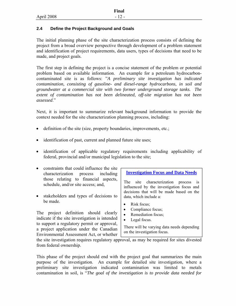
2.4 Define the Project Background and Goals

The initial planning phase of the site characterization process consists of defining the project from a broad overview perspective through development of a problem statement and identification of project requirements, data users, types of decisions that need to be made, and project goals.

The first step in defining the project is a concise statement of the problem or potential problem based on available information. An example for a petroleum hydrocarbon-contaminated site is as follows: ”A preliminary site investigation has indicated contamination, consisting of gasoline- and diesel-range hydrocarbons, in soil and groundwater at a commercial site with two former underground storage tanks. The extent of contamination has not been delineated, off-site migration has not been assessed.”

Next, it is important to summarize relevant background information to provide the context needed for the site characterization planning process, including:

• definition of the site (size, property boundaries, improvements, etc.;

• identification of past, current and planned future site uses;

• identification of applicable regulatory requirements including applicability of federal, provincial and/or municipal legislation to the site;

• constraints that could influence the site characterization process including those relating to financial aspects, schedule, and/or site access; and,

• stakeholders and types of decisions to be made.

The project definition should clearly indicate if the site investigation is intended to support a regulatory permit or approval, a project application under the Canadian Environmental Assessment Act, or whether the site investigation requires regulatory approval, as may be required for sites divested from federal ownership.

This phase of the project should end with the project goal that summarizes the main purpose of the investigation. An example for detailed site investigation, where a preliminary site investigation indicated contamination was limited to metals contamination in soil, is “The goal of the investigation is to provide data needed for

Investigation Focus and Data Needs

The site characterization process is influenced by the investigation focus and decisions that will be made based on the data, which include a:

• Risk focus; • Compliance focus; • Remediation focus; • Legal focus.

There will be varying data needs depending on the investigation focus.

April 2008 - 13 -

Final

human health risk assessment, which is delineation of the vertical and lateral extent of metals contamination, data on the contaminant distribution and relevant statistics, and supporting data on soil properties.”

The initial planning phase of the project will also involve assembling a team to perform the work. Often a multi-disciplinary team comprised of individuals with expertise in hydrogeology, environmental sampling and analysis, human health and/or ecological risk assessment, and statistics is assembled to complete risk assessments.

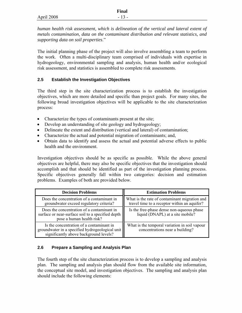
2.5 Establish the Investigation Objectives

The third step in the site characterization process is to establish the investigation objectives, which are more detailed and specific than project goals. For many sites, the following broad investigation objectives will be applicable to the site characterization process:

• Characterize the types of contaminants present at the site; • Develop an understanding of site geology and hydrogeology; • Delineate the extent and distribution (vertical and lateral) of contamination; • Characterize the actual and potential migration of contaminants; and, • Obtain data to identify and assess the actual and potential adverse effects to public

health and the environment.

Investigation objectives should be as specific as possible. While the above general objectives are helpful, there may also be specific objectives that the investigation should accomplish and that should be identified as part of the investigation planning process. Specific objectives generally fall within two categories: decision and estimation problems. Examples of both are provided below.

Decision Problems Estimation Problems Does the concentration of a contaminant in

groundwater exceed regulatory criteria? What is the rate of contaminant migration and

travel time to a receptor within an aquifer? Does the concentration of a contaminant in

surface or near-surface soil to a specified depth pose a human health risk?

Is the free-phase dense non-aqueous phase liquid (DNAPL) at a site mobile?

Is the concentration of a contaminant in groundwater in a specified hydrogeological unit

significantly above background levels?

What is the temporal variation in soil vapour concentrations near a building?

2.6 Prepare a Sampling and Analysis Plan

The fourth step of the site characterization process is to develop a sampling and analysis plan. The sampling and analysis plan should flow from the available site information, the conceptual site model, and investigation objectives. The sampling and analysis plan should include the following elements:

April 2008 - 14 -

Final

• Review of Existing Data; • Pre-mobilization Tasks; • Sampling Media, Data Types and Investigation Tools; • Sampling Design; • Sampling and Analysis Methods and Quality Assurance Project Plan. The scope of the sampling plan will vary depending on the project. The above elements of the sampling and analysis plan are described below.

2.6.1 Review of Existing Data

A critical review of available existing data is an essential first step for all projects. The data review is used to develop the CSM and guide the scoping of investigation programs. The review should be thorough and include an assessment of the reliability and usefulness of the data for the purposes of the current project. The review should clearly state which data have been relied upon. A review checklist for evaluating existing reports is provided in Volume 2 of this guidance.

2.6.2 Pre-mobilization Tasks

The pre-mobilization tasks include preparation of a project health and safety plan (HSP) and locating above-ground and below-ground utilities and structures that could affect or be affected by an intrusive investigation program.

The preparation and implementation of a project specific HSP is a critical part of the site characterization process to ensure that samping activities are conducted in a manner that will not compromise the health and safety of site workers, by-standers, or others. Use of existing site information and data should be considered in the development of the HSP. Sufficient reference material existing in the literature for developing HSPs therefore will not be discussed further as part of this guidance.

2.6.3 Sampling Media, Data Types and Investigation Tools

Site characterization for risk assessment may include sampling of several different media including soil, sediment, groundwater, soil vapour, indoor air, outdoor air, biota, surface water, indoor dust, and outdoor dust. The media addressed by this guidance are soil, groundwater, soil vapour and indoor air vapour.

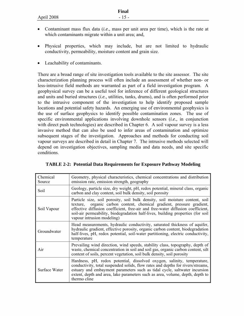
The different types of data that may be needed for risk assessment, in addition to chemical concentrations in each media, are summarized in Table 2-2. Several different types of data may be needed for site characterization purposes including:

• Chemical concentration data, which may be on a mass per unit weight or volume basis;

April 2008 - 15 -

Final

• Contaminant mass flux data (i.e., mass per unit area per time), which is the rate at which contaminants migrate within a unit area; and,

• Physical properties, which may include, but are not limited to hydraulic conductivity, permeability, moisture content and grain size.

• Leachability of contaminants.

There are a broad range of site investigation tools available to the site assessor. The site characterization planning process will often include an assessment of whether non- or less-intrusive field methods are warranted as part of a field investigation program. A geophysical survey can be a useful tool for inference of different geological structures and units and buried structures (i.e., utilities, tanks, drums), and is often performed prior to the intrusive component of the investigation to help identify proposed sample locations and potential safety hazards. An emerging use of environmental geophysics is the use of surface geophysics to identify possible contamination zones. The use of specific environmental applications involving downhole sensors (i.e., in conjunction with direct push technologies) are described in Chapter 6. A soil vapour survey is a less invasive method that can also be used to infer areas of contamination and optimize subsequent stages of the investigation. Approaches and methods for conducting soil vapour surveys are described in detail in Chapter 7. The intrusive methods selected will depend on investigation objectives, sampling media and data needs, and site specific conditions.

TABLE 2-2: Potential Data Requirements for Exposure Pathway Modeling

Chemical Source

Geometry, physical characteristics, chemical concentrations and distribution emission rate, emission strength, geography

Soil Geology, particle size, dry weight, pH, redox potential, mineral class, organic carbon and clay content, soil bulk density, soil porosity

Soil Vapour

Particle size, soil porosity, soil bulk density, soil moisture content, soil texture, organic carbon content, chemical gradient, pressure gradient, effective diffusion coefficient, free-air and free-water diffusion coefficient, soil-air permeability, biodegradation half-lives, building properties (for soil vapour intrusion modeling)

Groundwater Head measurements, hydraulic conductivity, saturated thickness of aquifer, hydraulic gradient, effective porosity, organic carbon content, biodegradation half-lives, pH, redox potential, soil-water partitioning, electric conductivity, temperature

Air Prevailing wind direction, wind speeds, stability class, topography, depth of waste, chemical concentration in soil and soil gas, organic carbon content, silt content of soils, percent vegetation, soil bulk density, soil porosity

Surface Water

Hardness, pH, redox potential, dissolved oxygen, salinity, temperature, conductivity, total suspended solids, flow rates and depths for rivers/streams, estuary and embayment parameters such as tidal cycle, saltwater incursion extent, depth and area, lake parameters such as area, volume, depth, depth to thermo cline

April 2008 - 16 -

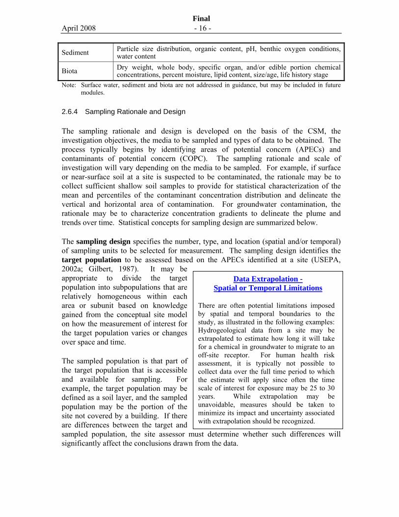
Final

Sediment Particle size distribution, organic content, pH, benthic oxygen conditions, water content

Biota Dry weight, whole body, specific organ, and/or edible portion chemical concentrations, percent moisture, lipid content, size/age, life history stage

Note: Surface water, sediment and biota are not addressed in guidance, but may be included in future modules.

2.6.4 Sampling Rationale and Design

The sampling rationale and design is developed on the basis of the CSM, the investigation objectives, the media to be sampled and types of data to be obtained. The process typically begins by identifying areas of potential concern (APECs) and contaminants of potential concern (COPC). The sampling rationale and scale of investigation will vary depending on the media to be sampled. For example, if surface or near-surface soil at a site is suspected to be contaminated, the rationale may be to collect sufficient shallow soil samples to provide for statistical characterization of the mean and percentiles of the contaminant concentration distribution and delineate the vertical and horizontal area of contamination. For groundwater contamination, the rationale may be to characterize concentration gradients to delineate the plume and trends over time. Statistical concepts for sampling design are summarized below.

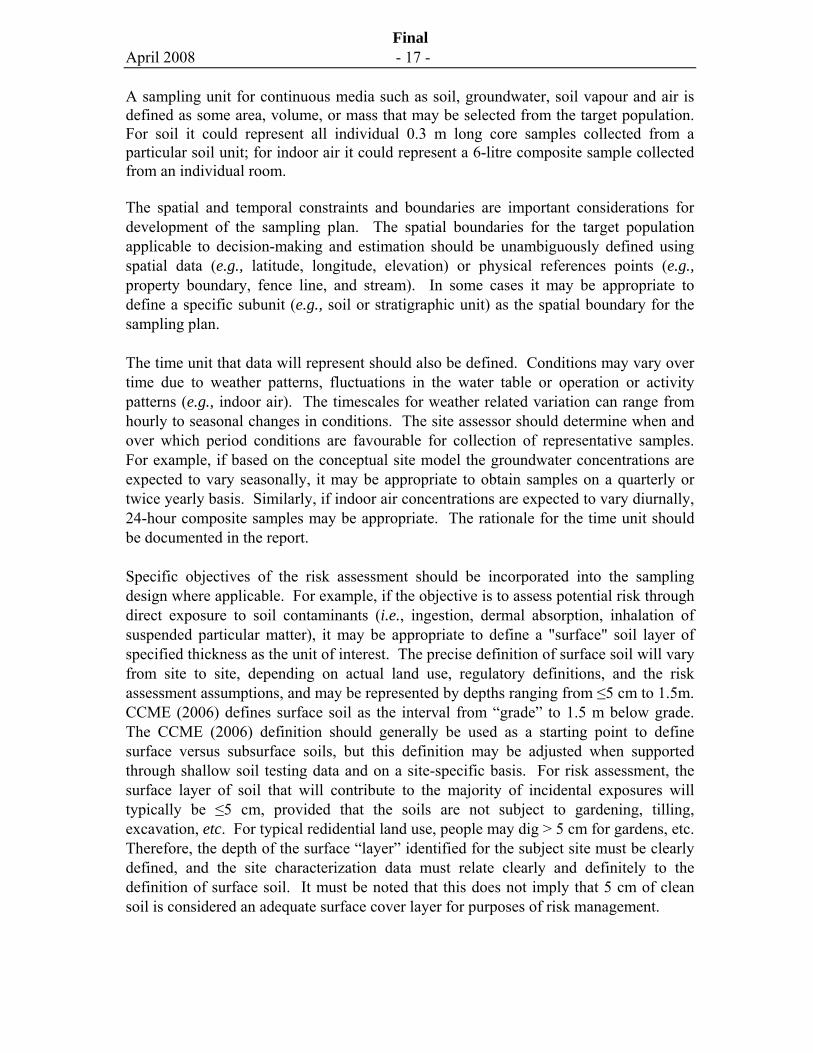
The sampling design specifies the number, type, and location (spatial and/or temporal) of sampling units to be selected for measurement. The sampling design identifies the target population to be assessed based on the APECs identified at a site (USEPA, 2002a; Gilbert, 1987). It may be appropriate to divide the target population into subpopulations that are relatively homogeneous within each area or subunit based on knowledge gained from the conceptual site model on how the measurement of interest for the target population varies or changes over space and time.

The sampled population is that part of the target population that is accessible and available for sampling. For example, the target population may be defined as a soil layer, and the sampled population may be the portion of the site not covered by a building. If there are differences between the target and sampled population, the site assessor must determine whether such differences will significantly affect the conclusions drawn from the data.

Data Extrapolation - Spatial or Temporal Limitations

There are often potential limitations imposed by spatial and temporal boundaries to the study, as illustrated in the following examples: Hydrogeological data from a site may be extrapolated to estimate how long it will take for a chemical in groundwater to migrate to an off-site receptor. For human health risk assessment, it is typically not possible to collect data over the full time period to which the estimate will apply since often the time scale of interest for exposure may be 25 to 30 years. While extrapolation may be unavoidable, measures should be taken to minimize its impact and uncertainty associated with extrapolation should be recognized.

April 2008 - 17 -

Final

A sampling unit for continuous media such as soil, groundwater, soil vapour and air is defined as some area, volume, or mass that may be selected from the target population. For soil it could represent all individual 0.3 m long core samples collected from a particular soil unit; for indoor air it could represent a 6-litre composite sample collected from an individual room.

The spatial and temporal constraints and boundaries are important considerations for development of the sampling plan. The spatial boundaries for the target population applicable to decision-making and estimation should be unambiguously defined using spatial data (e.g., latitude, longitude, elevation) or physical references points (e.g., property boundary, fence line, and stream). In some cases it may be appropriate to define a specific subunit (e.g., soil or stratigraphic unit) as the spatial boundary for the sampling plan.

The time unit that data will represent should also be defined. Conditions may vary over time due to weather patterns, fluctuations in the water table or operation or activity patterns (e.g., indoor air). The timescales for weather related variation can range from hourly to seasonal changes in conditions. The site assessor should determine when and over which period conditions are favourable for collection of representative samples. For example, if based on the conceptual site model the groundwater concentrations are expected to vary seasonally, it may be appropriate to obtain samples on a quarterly or twice yearly basis. Similarly, if indoor air concentrations are expected to vary diurnally, 24-hour composite samples may be appropriate. The rationale for the time unit should be documented in the report.

Specific objectives of the risk assessment should be incorporated into the sampling design where applicable. For example, if the objective is to assess potential risk through direct exposure to soil contaminants (i.e., ingestion, dermal absorption, inhalation of suspended particular matter), it may be appropriate to define a "surface" soil layer of specified thickness as the unit of interest. The precise definition of surface soil will vary from site to site, depending on actual land use, regulatory definitions, and the risk assessment assumptions, and may be represented by depths ranging from ≤5 cm to 1.5m. CCME (2006) defines surface soil as the interval from “grade” to 1.5 m below grade. The CCME (2006) definition should generally be used as a starting point to define surface versus subsurface soils, but this definition may be adjusted when supported through shallow soil testing data and on a site-specific basis. For risk assessment, the surface layer of soil that will contribute to the majority of incidental exposures will typically be ≤5 cm, provided that the soils are not subject to gardening, tilling, excavation, etc. For typical redidential land use, people may dig > 5 cm for gardens, etc. Therefore, the depth of the surface “layer” identified for the subject site must be clearly defined, and the site characterization data must relate clearly and definitely to the definition of surface soil. It must be noted that this does not imply that 5 cm of clean soil is considered an adequate surface cover layer for purposes of risk management.

April 2008 - 18 -

Final

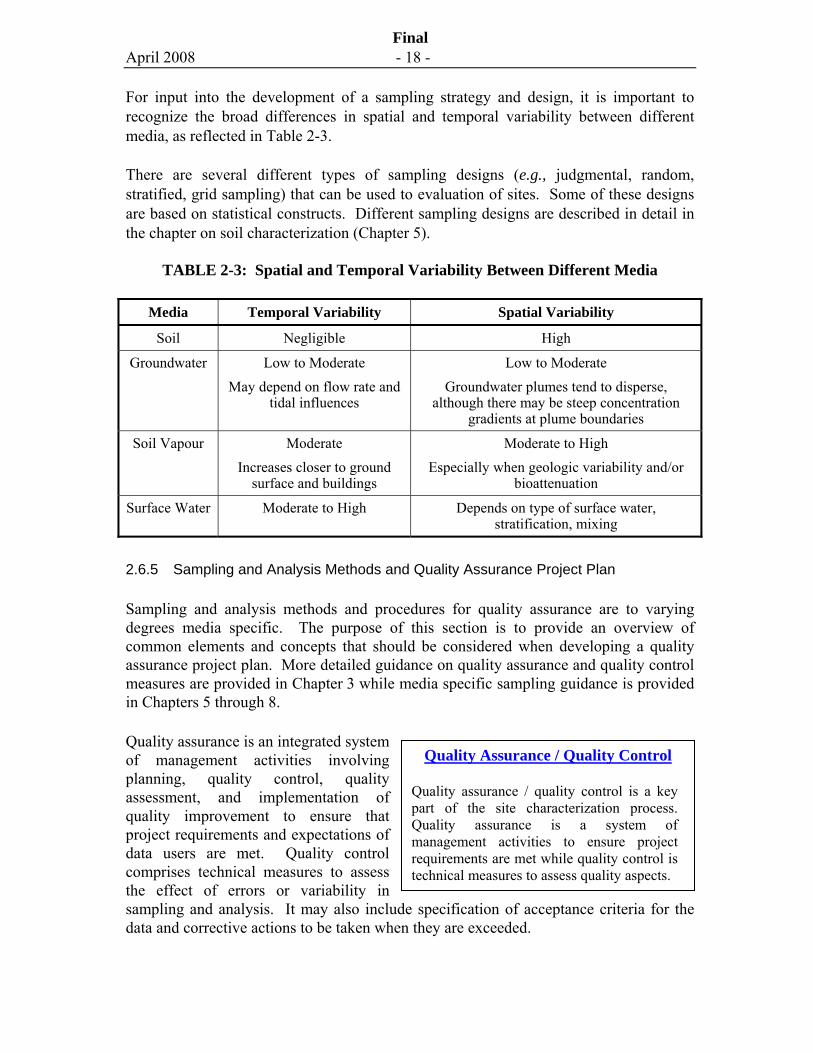
For input into the development of a sampling strategy and design, it is important to recognize the broad differences in spatial and temporal variability between different media, as reflected in Table 2-3.

There are several different types of sampling designs (e.g., judgmental, random, stratified, grid sampling) that can be used to evaluation of sites. Some of these designs are based on statistical constructs. Different sampling designs are described in detail in the chapter on soil characterization (Chapter 5).

TABLE 2-3: Spatial and Temporal Variability Between Different Media

Media Temporal Variability Spatial Variability

Soil Negligible High

Groundwater Low to Moderate May depend on flow rate and

tidal influences

Low to Moderate Groundwater plumes tend to disperse,

although there may be steep concentration gradients at plume boundaries

Soil Vapour Moderate Increases closer to ground

surface and buildings

Moderate to High Especially when geologic variability and/or

bioattenuation

Surface Water Moderate to High Depends on type of surface water, stratification, mixing

2.6.5 Sampling and Analysis Methods and Quality Assurance Project Plan

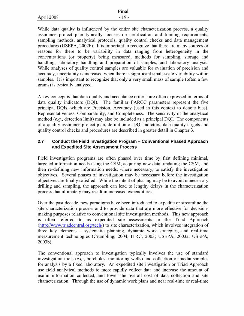
Sampling and analysis methods and procedures for quality assurance are to varying degrees media specific. The purpose of this section is to provide an overview of common elements and concepts that should be considered when developing a quality assurance project plan. More detailed guidance on quality assurance and quality control measures are provided in Chapter 3 while media specific sampling guidance is provided in Chapters 5 through 8.

Quality assurance is an integrated system of management activities involving planning, quality control, quality assessment, and implementation of quality improvement to ensure that project requirements and expectations of data users are met. Quality control comprises technical measures to assess the effect of errors or variability in sampling and analysis. It may also include specification of acceptance criteria for the data and corrective actions to be taken when they are exceeded.

Quality Assurance / Quality Control

Quality assurance / quality control is a key part of the site characterization process. Quality assurance is a system of management activities to ensure project requirements are met while quality control is technical measures to assess quality aspects.

April 2008 - 19 -

Final

While data quality is influenced by the entire site characterization process, a quality assurance project plan typically focuses on certification and training requirements, sampling methods, analytical protocols, quality control checks and data management procedures (USEPA, 2002b). It is important to recognize that there are many sources or reasons for there to be variability in data ranging from heterogeneity in the concentrations (or property) being measured, methods for sampling, storage and handling, laboratory handling and preparation of samples, and laboratory analysis. While analyses of quality control samples are valuable for evaluation of precision and accuracy, uncertainty is increased when there is significant small-scale variability within samples. It is important to recognize that only a very small mass of sample (often a few grams) is typically analyzed.

A key concept is that data quality and acceptance criteria are often expressed in terms of data quality indicators (DQI). The familiar PARCC parameters represent the five principal DQIs, which are Precision, Accuracy (used in this context to denote bias), Representativeness, Comparability, and Completeness. The sensitivity of the analytical method (e.g., detection limit) may also be included as a principal DQI. The components of a quality assurance project plan, definition of DQI indictors, data quality targets and quality control checks and procedures are described in greater detail in Chapter 3.

2.7 Conduct the Field Investigation Program – Conventional Phased Approach and Expedited Site Assessment Process

Field investigation programs are often phased over time by first defining minimal, targeted information needs using the CSM, acquiring new data, updating the CSM, and then re-defining new information needs, where necessary, to satisfy the investigation objectives. Several phases of investigation may be necessary before the investigation objectives are finally satisfied. While the intent of phasing may be to avoid unnecessary drilling and sampling, the approach can lead to lengthy delays in the characterization process that ultimately may result in increased expenditures.

Over the past decade, new paradigms have been introduced to expedite or streamline the site characterization process and to provide data that are more effective for decision-making purposes relative to conventional site investigation methods. This new approach is often referred to as expedited site assessments or the Triad Approach (http://www.triadcentral.org/tech/) to site characterization, which involves integration of three key elements – systematic planning, dynamic work strategies, and real-time measurement technologies (Crumbling, 2004; ITRC, 2003; USEPA, 2003a; USEPA, 2003b).

The conventional approach to investigation typically involves the use of standard investigation tools (e.g., boreholes, monitoring wells) and collection of media samples for analysis by a fixed laboratory. An expedited site investigation or Triad Approach use field analytical methods to more rapidly collect data and increase the amount of useful information collected, and lower the overall cost of data collection and site characterization. Through the use of dynamic work plans and near real-time or real-time

April 2008 - 20 -

Final

data collection and flexible contingency-based decision-making, there may be an opportunity to obtain better data in a more efficient manner that will more thoroughly describe site conditions.

The three principle components of the Triad Approach are summarized below:

• Systematic Planning. The systematic planning process is critical to the success of an expedited field investigation program. It involves the development of a CSM, a good understanding of the goals and objectives of the investigation, identification of roles and responsibilities of team members and development of a framework to support on-site decision-making, and identification of data quality requirements. While planning is important for any investigation, for expedited site assessments it is particularly important since field investigations will tend to evolve rapidly as they progress.

• Dynamic Work Strategies. The flexibility to change or adapt to information generated by real-time measurement technologies is key to dynamic work plans. The important decision points and logic should be identified together with contingent actions that may be required as the site investigation proceeds. Defined communication strategies are important for dynamic work strategies. Adequate resources should be allocated to data handling and interpretation to enable appropriate decisions to be made.

• Real-Time Measurement Technologies. Over the past decade there have been significant advancements in data collection technologies and measurement systems. A range of field analytical methods have been developed from rapid screening methods to on-site laboratories that provide nearly all the capabilities of a fixed laboratory, thus providing near real-time concentrations. The use of Global Positioning Systems provides for reasonably accurate determination of spatial locations. Through direct push technologies, there is the ability to rapidly collect multiple samples and provide concentration profiles. There are also an array of sensors that can be deployed with direct push technologies to help detect and delineate contamination zones. These new technological advances are important to the implementation of the Triad approach, and are discussed in subsequent chapters of this guidance.

A key concept is that the Triad Approach emphasizes managing decision uncertainty, rather than simply analytical uncertainty. For example, the Triad Approach recognizes that it may be more useful to obtain larger quantities of less precise data to characterize site conditions compared to a smaller quantity of more analytically precise data.

There are several requirements for successful implementation of a Triad Approach. There should be concurrence from regulators and stakeholders on data collection methods. It makes little sense to embark on a field investigation where data obtained will not meet minimum requirements. Likewise, there should be adequate quality control and assurance measures in-place. The team conducting the work should be

April 2008 - 21 -

Final

sufficiently experienced to make appropriate field decisions. There should be flexible contract provisions to facilitate the work.

2.8 Validate and Interpret Data

The sixth step of the site characterization process is the validation and interpretation of data. The data validation step involves review of whether the general objectives of the site investigation have been met, whether the quality assurance and quality control (QA/QC) results are within acceptable limits, and other checks to verify data and completeness. The PARCC parameters (Precision, Accuracy, Representativeness, Comparability, and Completeness) should be evaluated to determine whether performance and acceptance criteria have been met. A checklist for data validation is provided below:

� Are the data complete based on the sampling and analysis plan?

� Is the documentation complete including field data records, test pit, borehole and monitoring well logs, analytical laboratory reports, and all other supporting documentation?

� Have all test holes and sampling locations been clearly indicated on scaled drawings?

� Have the QA/QC data been reviewed and are they within acceptable limits? Are re-tests or verification tests required? Can the data be relied upon?

� Have apparent outliers been evaluated and addressed?

� Has the data been checked for possible transcription and manipulation errors?

� Have all APECs been adequately assessed for all COPCs?

� Have the investigation objectives been met, including all data required for risk assessment purposes?

� Has available previous work that can be reliably used been synthesized in the data interpretation?

� Have the sampling design objectives been met? Based on the updated conceptual site model, has sufficient sampling been completed at the site based on the study boundaries and APECs and populations identified?

� Do the results make sense relative to the conceptual site model and hypothesis for site contamination?

� Have the correct criteria or standards been used for all relevant media?

� Has off-site migration of contamination been identified?

April 2008 - 22 -

Final

� Is further assessment required to delineate the horizontal and/or vertical extent of contamination at a site?

The data interpretation will be specific to the type and quantity of data collected, the media being sampled and other project-specific considerations. Broadly applicable guidance and principles for data interpretation are provided below while additional considerations pertinent to the media under assessment (soil, groundwater and soil vapour) are addressed in the subsequent chapters.

Exploratory data analysis should be completed through techniques that provide information on trends, correlations and other patterns. Several exploratory data views are listed below:

• Data posting to show concentration patterns in plan view and cross section; • Frequency tables; • Histograms; • Cumulative frequency plots; • Correlation plots; and, • Contouring.

If the site is likely to proceed to human health risk assessment (HHRA), basic statistical parameters should be calculated for each data set (e.g., number of samples, minimum, maximum, arithmetic mean, standard deviation, coefficient of variation, percentiles of the distribution). For this purpose, the data must be grouped into logical groupings that reflect study boundaries, the CSM, and areas of potential concern. To the extent possible, the data should represent a single population, although in some cases, statistical analyses may be needed to determine appropriate groupings of data and possible outliers.

Statistical parameters can be grouped into non-parametric statistics such as the minimum, maximum, median and percentiles of the data set, and parametric statistics such as the upper confidence limit of the mean, which often assume a normally-distributed data set, although as indicated in Gilbert (1987), there are also methods for log-normal data. Since environmental data sets are often skewed and follow an approximate log-normal distribution, data sets should be carefully evaluated as to their underlying distribution since the use of conventional statistical parameters such as the arithmetic mean and standard deviation may result in biased estimates (Gilbert, 1987). Further guidance on statistical evaluation of soil data is provided in Chapter 5. Although high concentration values may appear to be anomalous, great care must be taken when considering whether to remove apparent outliers from a data set. Such data may represent hot-spots that comprise a separate population.

2.9 Resources and Weblinks

Environment Canada Technical Assistance Bulletins (TAB): Twenty-nine bulletins provide useful background information on site assessment process, sampling and

April 2008 - 23 -

Final

analysis procedures, remediation technologies, and expedited site characterization tools. http://www.on.ec.gc.ca/pollution/ecnpd/contaminassist_e.html

U.S. Environmental Protection Agency: The USEPA has extensive resources available on their Hazardous Waste Clean-up Information (CLU-IN) website. General publications and training course on site assessment and remediation can be found at http://www.clu-in.org/techdrct/techpubs.asp. The USEPA Technology Innovation program has a website specific to characterization and monitoring technologies http://cluin.org/char1_edu.cfm and a monthly newsletter (subscribe at http://www.epa.gov/tio/techdrct/. Information on the USEPA Superfund program and links to an extensive document library can be found at http://www.epa.gov/superfund/about.htm. Guidance specific to investigation and clean-up of Brownfield’s sites can be found at http://www.epa.gov/swerosps/bf/.

Conceptual Site Models: An example of a complete CSM including diagrams prepared for soil screening purposes can be found in Attachment A of the Soil Screening Guidance: User’s Guide (USEPA, 1996). http://www.epa.gov/superfund/health/conmedia/soil/pdfs/attacha.pdf

Conceptual Exposure Models: A software application, the “Site Conceptual Exposure Model Builder” that can generate conceptual exposure model (CEM) diagrams, but that also helps understand site data and fate and transport mechanisms has been developed by the U.S. Department of Energy. http://homer.ornl.gov/nuclearsafety/nsea/oepa/tools/scemman.pdf

2.10 References

American Society for Testing and Materials Standards (ASTM) E1527-06 (2005). Standard Practice for Environmental Site Assessments: Phase 1 Environmental Site Assessment Process. ASTM International, 27 pages.

American Society for Testing and Materials Standards (ASTM) E1903-97 (2002) Standard Guide for Environmental Site Assessments: Phase II Environmental Site Assessment Process, ASTM International, 14 pages.

Canadian Council of Ministers of the Environment (CCME), 2006. A Protocol for the Derivation of Environmental and Human Health Soil Quality Guidelines, ISBN-10 1-896997-45-7 PDF ISBN-13 978-1-896997-45-2 PDF, PN 1332

CAN/CSA-Z768-01, 2001. Phase 1 Environmental Site Assessment.

CAN/CSA-Z769-00, 2000. Phase II Environmental Site Assessment.

Crumbling, D.M. 2004. The Triad Approach to Managing the Uncertainty in Environmental Data. White paper prepared for United States Environmental Protection Agency. March 25.

April 2008 - 24 -

Final

Gilbert, R.O. 1987. Statistical Methods for Environmental Pollution Monitoring. Van Nostrand Reinhold Company, New York, NY. 320 pp.

Hers, I. and R. Zapf-Gilje, 1991, The Use of Statistics for Interpretation of Soil Contamination at the Former Expo '86 Site, Preprints, 44th Canadian Geotechnical Conference, Calgary.

Interstate Technology & Regulatory Council (ITRC), 2003. Technical and Regulatory Guidance for the Triad Approach: A New Paradigm for Environmental Project Management, Prepared by Sampling, Characterization and Monitoring Team, December.

Starks, T. H. 1986. Determination of Support in Soil Sampling. Mathematical Geology, Vol. 18, No. 6, pp. 529-537.

U.S. Environmental Protection Agency, 2006. Guidance on Systematic Planning Using the Data Quality Objectives Process EPA QA/G-4. Office of Environmental Information Washington, DC 20460, Report EPA/240/B-06/001, February.

U.S. Environmental Protection Agency, 2003a. Using Dynamic Field Activities for On-Site Decision Making: A Guide for Project Managers. Office of Solid Waste and Emergency Response U.S. Environmental Protection Agency Washington, DC 20460, OSWER Report No. 9200.1-40 EPA/540/R-03/002, May.

U.S. Environmental Protection Agency, 2003b. Using the Triad Approach to Streamline Brownfield’s Site Assessment and Cleanup – Brownfield’s Technology Primer Series. Office of Solid Waste and Emergency Response Brownfield’s Technology Support Center Washington, DC 20460, June.

U.S. Environmental Protection Agency, 2002a. Guidance on Choosing a Sampling Design for Environmental Data Collection for Use in Developing a Quality Assurance Project Plan, Washington, DC 20460. Report EPA QA/G-5S, December.

U.S. Environmental Protection Agency, 2002b. Guidance for Quality Assurance Project Plans. Washington, DC, Report EPA/240/R-02/009, December.

U.S. Environmental Protection Agency, 1996. Soil Screening Guidance: User’s Guide. United States Office of Solid Waste and Publication 9355.4-23. Washington, DC, July.

April 2008 - 25 -

Final

3.0 QUALITY ASSURANCE/QUALITY CONTROL

The goal of representative sampling is to collect samples which will yield results that accurately characterize site conditions. The goal of quality assurance and quality control (QA/QC) is to limit errors and bias in sampling and analysis through integrated implementation of management, assessment and control measures, thus facilitating generation of data that are useful for their intended purpose. This section begins with a description of the quality assurance project plan components, which is an important planning phase that helps ensure acceptable data quality. Next, data quality indicators and targets are discussed, followed by specific data quality control checks and procedures.

3.1 Quality Assurance Project Plan

The quality assurance project plan (QAPP) is an integral part of a sampling and analysis plan. The QAPP identifies all aspects of the site characterization program that may influence data quality. The components of a QAPP are summarized in Table 3-1. Many aspects of the QAPP are media and method specific, and relevant protocols should be consulted for details (USEPA, 2002).

The QAPP should include consideration of laboratory accreditation and analytical protocols. Laboratories should be accredited to the international standard "ANS/ISO/IEC 17025 General Requirements for the Competence of Testing and Calibration Laboratories". An accredited laboratory will have a "scope of accreditation" that lists the matrix, method and parameters for which a laboratory has been accredited (many laboratories also conduct analyses that are not on their scope of accreditation meaning they are not accredited for those tests). There are two recognized agencies in Canada granting accreditation to environmental testing laboratories: (i) the Canadian Association for Environmental Analytical Laboratories (CAEAL), and (ii) Standards Council of Canada (SCC). Standardised methods are typically used for analysis of many chemical parameters, as published in the following documents (refer to the most recent updates):

• Test Methods for Evaluating Solid Waste; SW-846. Published by United States Environmental Protection Agency (USEPA).

• Methods for Chemical Analysis of Water and Wastes (MCAWW). Published by United States Environmental Protection Agency (USEPA).

• Standard Methods for the Examination of Water and Wastewater. Published by the American Public Health Association (APHA).

• Annual Book of ASTM Standards, Section 11 - Water and Environmental Technology. Published by the American Society for Testing and Materials (ASTM).

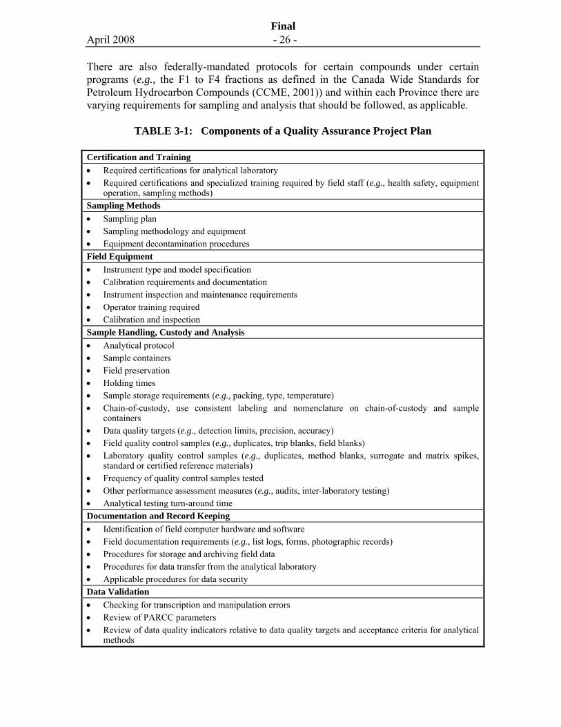
April 2008 - 26 -

Final

There are also federally-mandated protocols for certain compounds under certain programs (e.g., the F1 to F4 fractions as defined in the Canada Wide Standards for Petroleum Hydrocarbon Compounds (CCME, 2001)) and within each Province there are varying requirements for sampling and analysis that should be followed, as applicable.

TABLE 3-1: Components of a Quality Assurance Project Plan

Certification and Training • Required certifications for analytical laboratory • Required certifications and specialized training required by field staff (e.g., health safety, equipment

operation, sampling methods) Sampling Methods • Sampling plan • Sampling methodology and equipment • Equipment decontamination procedures Field Equipment • Instrument type and model specification • Calibration requirements and documentation • Instrument inspection and maintenance requirements • Operator training required • Calibration and inspection Sample Handling, Custody and Analysis • Analytical protocol • Sample containers • Field preservation • Holding times • Sample storage requirements (e.g., packing, type, temperature) • Chain-of-custody, use consistent labeling and nomenclature on chain-of-custody and sample

containers • Data quality targets (e.g., detection limits, precision, accuracy) • Field quality control samples (e.g., duplicates, trip blanks, field blanks) • Laboratory quality control samples (e.g., duplicates, method blanks, surrogate and matrix spikes,

standard or certified reference materials) • Frequency of quality control samples tested • Other performance assessment measures (e.g., audits, inter-laboratory testing) • Analytical testing turn-around time Documentation and Record Keeping • Identification of field computer hardware and software • Field documentation requirements (e.g., list logs, forms, photographic records) • Procedures for storage and archiving field data • Procedures for data transfer from the analytical laboratory • Applicable procedures for data security Data Validation • Checking for transcription and manipulation errors • Review of PARCC parameters • Review of data quality indicators relative to data quality targets and acceptance criteria for analytical

methods

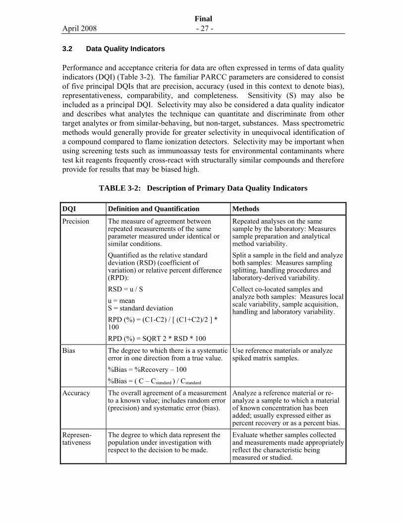
April 2008 - 27 -

Final

3.2 Data Quality Indicators

Performance and acceptance criteria for data are often expressed in terms of data quality indicators (DQI) (Table 3-2). The familiar PARCC parameters are considered to consist of five principal DQIs that are precision, accuracy (used in this context to denote bias), representativeness, comparability, and completeness. Sensitivity (S) may also be included as a principal DQI. Selectivity may also be considered a data quality indicator and describes what analytes the technique can quantitate and discriminate from other target analytes or from similar-behaving, but non-target, substances. Mass spectrometric methods would generally provide for greater selectivity in unequivocal identification of a compound compared to flame ionization detectors. Selectivity may be important when using screening tests such as immunoassay tests for environmental contaminants where test kit reagents frequently cross-react with structurally similar compounds and therefore provide for results that may be biased high.

TABLE 3-2: Description of Primary Data Quality Indicators

DQI Definition and Quantification Methods

Precision The measure of agreement between repeated measurements of the same parameter measured under identical or similar conditions. Quantified as the relative standard deviation (RSD) (coefficient of variation) or relative percent difference (RPD): RSD = u / S u = mean S = standard deviation RPD (%) = (C1-C2) / [ (C1+C2)/2 ] * 100 RPD (%) = SQRT 2 * RSD * 100

Repeated analyses on the same sample by the laboratory: Measures sample preparation and analytical method variability. Split a sample in the field and analyze both samples: Measures sampling splitting, handling procedures and laboratory-derived variability. Collect co-located samples and analyze both samples: Measures local scale variability, sample acquisition, handling and laboratory variability.

Bias The degree to which there is a systematic error in one direction from a true value. %Bias = %Recovery – 100 %Bias = ( C – Cstandard ) / Cstandard

Use reference materials or analyze spiked matrix samples.

Accuracy The overall agreement of a measurement to a known value; includes random error (precision) and systematic error (bias).

Analyze a reference material or re-analyze a sample to which a material of known concentration has been added; usually expressed either as percent recovery or as a percent bias.

Represen-tativeness

The degree to which data represent the population under investigation with respect to the decision to be made.

Evaluate whether samples collected and measurements made appropriately reflect the characteristic being measured or studied.

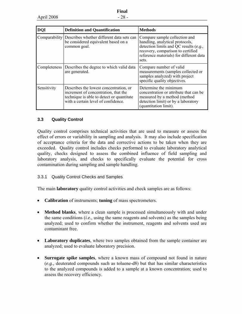
April 2008 - 28 -

Final

DQI Definition and Quantification Methods

Comparability Describes whether different data sets can be considered equivalent based on a common goal.

Compare sample collection and handling, analytical protocols, detection limits and QC results (e.g., recovery, comparison to certified reference materials) for different data sets.

Completeness Describes the degree to which valid data are generated.

Compare number of valid measurements (samples collected or samples analyzed) with project specific quality objectives.

Sensitivity Describes the lowest concentration, or increment of concentration, that the technique is able to detect or quantitate with a certain level of confidence.

Determine the minimum concentration or attribute that can be measured by a method (method detection limit) or by a laboratory (quantitation limit).

3.3 Quality Control

Quality control comprises technical activities that are used to measure or assess the effect of errors or variability in sampling and analysis. It may also include specification of acceptance criteria for the data and corrective actions to be taken when they are exceeded. Quality control includes checks performed to evaluate laboratory analytical quality, checks designed to assess the combined influence of field sampling and laboratory analysis, and checks to specifically evaluate the potential for cross contamination during sampling and sample handling.

3.3.1 Quality Control Checks and Samples

The main laboratory quality control activities and check samples are as follows:

• Calibration of instruments; tuning of mass spectrometers.

• Method blanks, where a clean sample is processed simultaneously with and under the same conditions (i.e., using the same reagents and solvents) as the samples being analyzed; used to confirm whether the instrument, reagents and solvents used are contaminant free.

• Laboratory duplicates, where two samples obtained from the sample container are analyzed; used to evaluate laboratory precision.

• Surrogate spike samples, where a known mass of compound not found in nature (e.g., deuterated compounds such as toluene-d8) but that has similar characteristics to the analyzed compounds is added to a sample at a known concentration; used to assess the recovery efficiency.

April 2008 - 29 -

Final

• Matrix spike samples, where a known mass of target analyte is added to a matrix sample with known concentrations; used to evaluate the influence of the matrix on a method’s recovery efficiency.

• Standard or certified reference materials, a reference material where the content or concentration has been established to a very high level of certainty (usually by a national regulatory agency); used to assess accuracy.

The main field quality control checks are as follows:

• Field duplicates, where split samples or co-located samples obtained in the field using the same sampling procedure are submitted to the laboratory “blind”; used to assess sampling and analysis precision.

• Trip blanks, where a clean sample of the matrix being analyzed is transported to and from the site using the same container as the samples analyzed; used to assess whether cross-contamination occurred during sample transport and storage.

• Equipment blanks, prepared in the field, where for example, contaminant-free water (distilled-deionized) or air is passed through a sampling device (e.g., pump and tubing); used to assess equipment decontamination procedures.

• Field blanks, which can consist of a clean sample (e.g., distilled-deionized water) where the sample container is exposed to sampling conditions (i.e., cap removed) or where an ambient air sample is obtained; used to check for artifacts introduced by background conditions.

Field control checks should be completed early in the site investigation process so that adjustments can be made, when warranted.

3.3.2 Recommended Minimum Frequency of Quality Control Samples

The recommended minimum frequency for testing of field and laboratory duplicate samples is 1 in 10 samples analyzed for both field and laboratory tests, although for smaller programs where less than ten samples are analyzed, consideration should nevertheless be given to analysis of a duplicate sample. The samples submitted for duplicate analysis should have sufficiently high levels of contamination (if possible) so that there is the ability to evaluate precision. For other quality control samples, it is recommended that one check sample per 10 to 20 samples be analyzed.

April 2008 - 30 -

Final

3.4 Data Quality Targets

The previous sections described the data quality indicators used to evaluate precision and accuracy and the specific quality control checks that are performed to evaluate data quality. As part of the quality assurance project plan, it is also important to establish data quality targets or to recognize method precision and accuracy that can be achieved based on the analytical method and matrix being tested.

Most analytical methods such as those published in the USEPA SW-846 compendium of methods include acceptance criteria for quality control tests. For example, for USEPA Method 8260B (VOCs by GC/MS), the required precision of calibration checks is a RSD of 15 percent for target analytes and 30 percent for calibration check compounds (CCCs). The acceptable recoveries for quality control tests for Method 8260B are as follows:

• Matrix spike: Water: 65-135% Soil: 50-150%

• Surrogate spike: Water 85-115% Soil: 70-125%

• Standard or certified reference material: Water: 70-130% Soil: 65-135%

Typically, laboratories adopt or establish their own acceptance criteria that are to varying degrees based on performance requirements in the applicable analytical protocols (e.g., USEPA SW-846). As a general rule, the allowable tolerances for soil are greater than for groundwater due to variability introduced by the matrix. Similarly, for semi-volatiles, the ranges for acceptable recoveries are slightly higher than for volatiles.

The data quality targets should be compared to analytical method performance specifications. The analytical detection limit (practical quantification limit) is a basic data quality requirement, and often the target is set at a minimum of 5X to 10X less than the regulatory criteria. An example data quality target for a project might read as

Detection Limits

While there are many different definitions for detection limits, the primary definitions that may be relevant to practitioners are:

Method detection limit (MDL): The minimum concentration of an analyte that can be measured and reported with 99% confidence to be greater than zero for a given matrix and specific method.

Limit of Quantification (LOQ): The lowest concentration of an analyte that can be reliably measured within specified limits of precision and accuracy during routine operating conditions, as opposed to being detected (USEPA, 2002; Gibbons and Coleman, 2001).

Practical Quantification Limit (PQL): May be similarly defined as the LOQ, the reporting limits in the method, or otherwise defined.

Laboratory reporting limit (LRL): The lowest concentration of an analyte reported within a reasonable degree of accuracy and precision, often synonymous with the LOQ or PQL. The LRL is typically 3-10 times the MDL.

The uncertainty in concentrations increases near to the detection limit. Some laboratories may also report concentrations detected below the LRL (“J-flagged” results); however, these concentrations should be considered an estimate. Detection limits may be raised due to the matrix effects or sample dilution.

April 2008 - 31 -

Final

follows: “The measurement method selected for the project must be able to detect the presence of compounds X, Y, and Z in groundwater at a quantitation limit of 1 ug/L with a recovery range (relative to certified reference materials) of 70 to 130 percent and a precision, as quantified by the RSD, of less than 20 percent”.

3.4.1 Duplicate Samples

Sampling programs should include both analyses of laboratory and field duplicate samples. The acceptance criteria will depend on the analytical protocol and media, but guidelines are provided below for common analytes (extractable hydrocarbons, metals, and volatile and semi-volatile organic chemicals).

For laboratory duplicates of groundwater, the RSD should be less than 15 to 20 percent, which corresponds to a RPD of less than 21 to 28 percent. For soil there is greater matrix variability; therefore, somewhat higher acceptable RSDs on the order of 20 to 30 percent are reasonable.

For field duplicates, there is added variability introduced by matrix variability and sampling and handling procedures. Quantifying acceptable precision is a matter of judgment, but assuming the field and laboratory error are similar in magnitude, acceptance criteria twice those given above would result (i.e., RSD of 30 to 40 percent for groundwater and 40 to 60 percent for soil).

Near to the detection limit, acceptance criteria are relaxed, for example, within 5X of the detection limit, a criterion that may be used is that the difference between the duplicate concentrations should be less than 2X the detection limit. When the acceptance criteria are exceeded, the sampling procedures should be reviewed and the soil or groundwater matrix examined. The importance of reduced precision becomes more important when concentrations straddle or are near regulatory guidelines.

Limit of Quantitation (LOQ) - Smallest analyte concentration for which the variability (95% confidence limit) does not exceed approximately 30% of the analyte concentration. Some agencies define the LOQ to be n times the detection limit.

3.5 Reporting of QA/QC

The results of the QA/QC program represent an important part of the site characterization report. The QA/QC section of the report (or appendices) should include the following information:

� Are the data complete based on the sampling and analysis plan?

� Specifications and calibration records for field equipment used;

April 2008 - 32 -

Final

� Field staff who conducted the sampling and verification of training where warranted;

� Sampling equipment used and decontamination procedures and protocols that were followed during sampling;

� Laboratory that conducted the analyses and certification for parameters analyzed;

� Sampling containers and field preservatives used;

� Sample storage and transportation procedures;

� Analytical methods, detection limits and chain-of-custody forms;

� Whether holding times were met;

� The data quality targets specified in the sampling plan (e.g., detection limits, precision, accuracy);

� The results of field and laboratory quality control check tests (e.g., duplicates, spikes, surrogates, blanks);

� Calculation of data quality indicators (e.g., RPD) for field and laboratory duplicate samples;

� Discussion of departures from the sampling plan and rationale and anticipated impact on results; and,

� Conclusions on the reliability of the data based on the results of the QA/QC program.

3.6 References

American Public Health Association (APHA), see latest update. Standard Methods for the Examination of Water and Wastewater.

American Society for Testing and Materials (ASTM), see latest update. Annual Book of ASTM Standards, Section 11 - Water and Environmental Technology.

Canadian Council of Ministers of the Environment, 2001. Canada-Wide Standards for Petroleum Hydrocarbon (PHC) in Soil. Endorsed by CCME Council of Ministers, April 30-May 1, 2001, Winnipeg.

Gibbons, R.G. and D.E. Coleman, 2001. Statistical Methods for Detection and Quantification of Environmental Contamination. Wiley, 400 pages, July.

U.S. Environmental Protection Agency, 2002. Guidance for Quality Assurance Project Plans. Report EPA/240/R-02/009. Washington, DC, December 2002. see additional documents: http://www.epa.gov/quality/qapps.html

April 2008 - 33 -

Final

U.S. Environmental Protection Agency, see latest update. Test Methods for Evaluating Solid Waste; SW-846. http://www.epa.gov/epaoswer/hazwaste/test/main.htm

U.S. Environmental Protection Agency, see latest update. Methods for Chemical Analysis of Water and Wastes (MCAWW). http://www.ntis.gov/products/epa-water-methods.aspx

April 2008 - 34 -

Final

4.0 CONCEPTUAL SITE MODEL FOR CONTAMINATED SITES

As described in Chapter 2, a conceptual site model (CSM) provides a visual representation and narrative description of the contamination sources and physical, chemical, and biological processes occurring, or that have occurred, at a contaminated site that should be continuously updated as new information is obtained. It is essential that the different potential types of contamination and their fate and transport characteristics be understood for the development of the CSM. The purpose of this chapter is to describe these characteristics and facilitate informed and effective planning of site investigation programs.

This chapter is divided into three parts: (1) the sources and types of chemicals that may be found at contaminated sites, (2) the processes for fate and transport of chemicals in the unsaturated zone and groundwater that are relevant to receptors exposed to groundwater (“groundwater pathway”), and (3) the processes for fate and transport of soil vapour that are relevant to receptors exposed to vapours (“soil vapour intrusion pathway”). The discussions on groundwater and vapour intrusion pathways are written from a risk perspective. The section on groundwater, in particular, is limited to an overview of key processes and issues. It is not intended to provide the theoretical background needed to understand groundwater flow and chemical transport processes, since this information is readily available elsewhere (e.g., Fetter, 2004; Domenico and Schwartz, 1998; Zheng and Bennett, 1995).

4.1 Contamination Sources and Types

4.1.1 Overview

There are a broad range of sources of soil, groundwater, soil vapour and indoor air contamination that comprise point sources and distributed, or non-point sources. Leaking fuel storage tanks, accidental spills at industrial sites, waste disposal areas, and landfills are examples of point sources of contamination; in contrast, the infiltration of water containing fertilizer applied to farmland or salt from road run-off represent non-point sources of contamination. The contaminants of concern may be man-made organic or inorganic chemicals or naturally occurring elements, such as arsenic or radionuclides, microbiological contaminants, and nitrates from agricultural sources.

Many contaminants biodegrade under natural conditions. Some breakdown or daughter products are innocuous (e.g. water, carbon dioxide) wheras some contaminants degrade to products that are more toxic and mobile than the source contaminant (e.g. vinyl chloride). Identification of potential contaminants of concern must be extended to the identification of potential breakdown products.

April 2008 - 35 -

Final

4.1.2 Common Types of Contamination

Common types and sources of contamination include petroleum hydrocarbon compounds (fuel products, lubricants, oil), polycyclic aromatic hydrocarbons (creosote, coal-tar), chlorinated solvents (degreasers, dry cleaners), non-chlorinated solvents (mineral spirits, naphtha’s), chlorophenols (wood preservatives), polychlorinated biphenyls (electrical equipment, hydraulic oil) and metals (mine waste dumps, wood treatment, metal plating). A list of land uses and activities that have been found to cause contamination and the types or classes of chemicals that may be associated with these land uses and activities is provided in Table 4-1.

Since sources and types of contaminants can be highly variable and complex, the information in Table 4-1 should only be used as a guide. Site assessors should conduct their own assessment of the potential for site activities to cause contamination and potential contaminants of concern. For site investigation planning, it is important to understand contamination sources and the types and properties of chemicals that may be present. While not intended to be exhaustive, several common types of contamination are described below to illustrate the range of chemical composition and properties that should be considered.

Petroleum hydrocarbon contamination is found at many sites with leaking above-ground or underground fuel storage tanks or distribution lines (e.g., gas stations, bulk plants, refineries or other fuel-handling facilities). Petroleum products can range from light distillate (e.g., gasoline), light to middle distillate (e.g., kerosene, Jet A, Jet B), middle distillate (e.g., diesel, Fuel Oil No. 2) to heavy distillate products (e.g., Fuel Oil No. 6).

Historically, some gasoline included additives such as tetra-ethyl lead, and less commonly ethylene dibromide and 1,2-dichloroethane (Falta et al., 2005). More recently, fuel oxygenates such as methyl tert-butyl ether (MTBE), tertiary-butyl alcohol (TBA) (a fuel oxygenate and also a breakdown product of MTBE), tert-amyl methyl ether (TAME) and ethanol have been added to fuels.

There are important physical, chemical and biological properties associated with additives. For example, MTBE is a relatively soluble compound and less amenable to biodegradation than benzene, ethylbenzene, toluene, and xylenes (BTEX). Higher quantities of ethanol may result in mobilization of residual NAPL and enhanced solubility of BTEX.

Coal tar contamination is often found at manufactured gas plant (MGP) sites historically used for the production of gas (for heating and illumination purposes) through the coal-gasification process. Creosote, which is a common wood preservative, is a distillation product of coal tar with a somewhat narrower range of compounds than coal tar. Both coal tar and creosote are composed of a complex mixture of polycyclic aromatic hydrocarbons (PAHs), typically representing about 85 percent of the compounds present, with lesser quantities of Alkyl-PAHs, monocyclic aromatic hydrocarbons

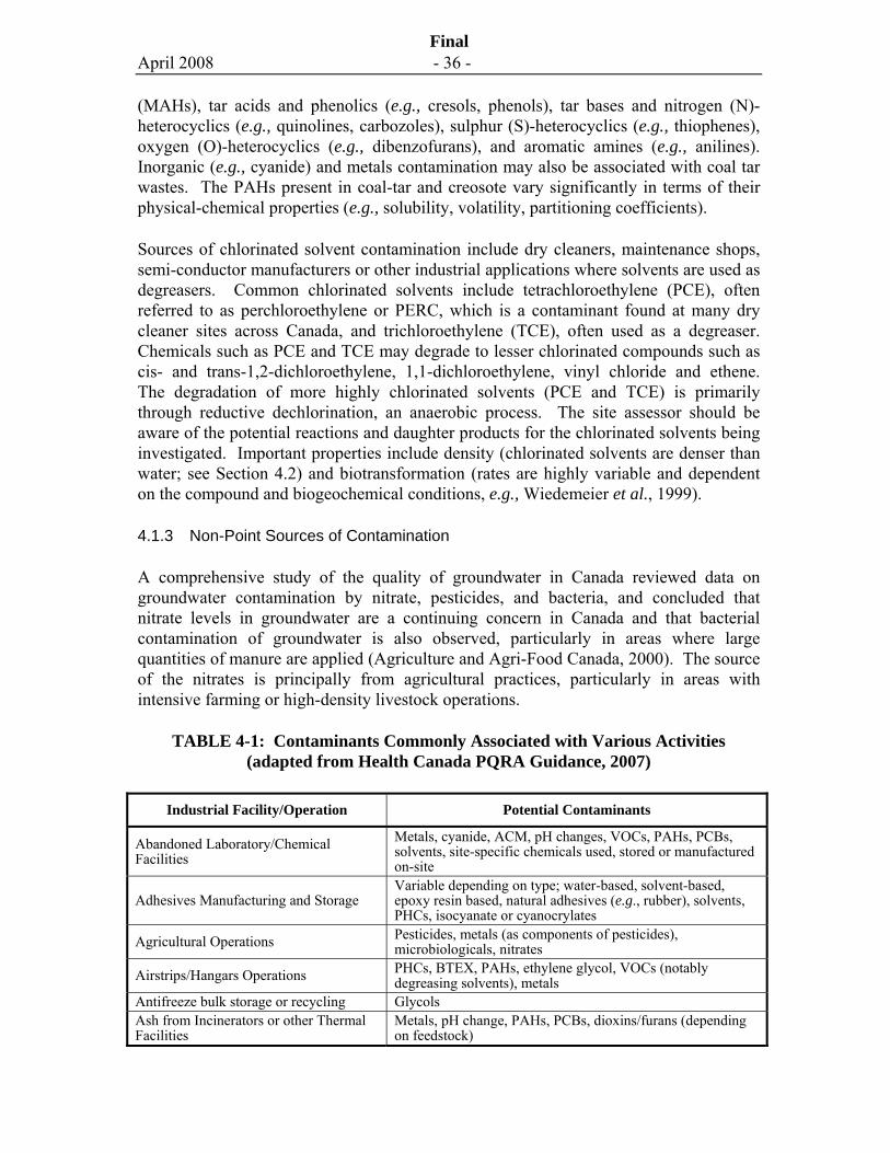
April 2008 - 36 -

Final

(MAHs), tar acids and phenolics (e.g., cresols, phenols), tar bases and nitrogen (N)-heterocyclics (e.g., quinolines, carbozoles), sulphur (S)-heterocyclics (e.g., thiophenes), oxygen (O)-heterocyclics (e.g., dibenzofurans), and aromatic amines (e.g., anilines). Inorganic (e.g., cyanide) and metals contamination may also be associated with coal tar wastes. The PAHs present in coal-tar and creosote vary significantly in terms of their physical-chemical properties (e.g., solubility, volatility, partitioning coefficients).

Sources of chlorinated solvent contamination include dry cleaners, maintenance shops, semi-conductor manufacturers or other industrial applications where solvents are used as degreasers. Common chlorinated solvents include tetrachloroethylene (PCE), often referred to as perchloroethylene or PERC, which is a contaminant found at many dry cleaner sites across Canada, and trichloroethylene (TCE), often used as a degreaser. Chemicals such as PCE and TCE may degrade to lesser chlorinated compounds such as cis- and trans-1,2-dichloroethylene, 1,1-dichloroethylene, vinyl chloride and ethene. The degradation of more highly chlorinated solvents (PCE and TCE) is primarily through reductive dechlorination, an anaerobic process. The site assessor should be aware of the potential reactions and daughter products for the chlorinated solvents being investigated. Important properties include density (chlorinated solvents are denser than water; see Section 4.2) and biotransformation (rates are highly variable and dependent on the compound and biogeochemical conditions, e.g., Wiedemeier et al., 1999).

4.1.3 Non-Point Sources of Contamination

A comprehensive study of the quality of groundwater in Canada reviewed data on groundwater contamination by nitrate, pesticides, and bacteria, and concluded that nitrate levels in groundwater are a continuing concern in Canada and that bacterial contamination of groundwater is also observed, particularly in areas where large quantities of manure are applied (Agriculture and Agri-Food Canada, 2000). The source of the nitrates is principally from agricultural practices, particularly in areas with intensive farming or high-density livestock operations.

TABLE 4-1: Contaminants Commonly Associated with Various Activities (adapted from Health Canada PQRA Guidance, 2007)

Industrial Facility/Operation Potential Contaminants

Abandoned Laboratory/Chemical Facilities

Metals, cyanide, ACM, pH changes, VOCs, PAHs, PCBs, solvents, site-specific chemicals used, stored or manufactured on-site

Adhesives Manufacturing and Storage Variable depending on type; water-based, solvent-based, epoxy resin based, natural adhesives (e.g., rubber), solvents, PHCs, isocyanate or cyanocrylates

Agricultural Operations Pesticides, metals (as components of pesticides), microbiologicals, nitrates

Airstrips/Hangars Operations PHCs, BTEX, PAHs, ethylene glycol, VOCs (notably degreasing solvents), metals

Antifreeze bulk storage or recycling Glycols Ash from Incinerators or other Thermal Facilities

Metals, pH change, PAHs, PCBs, dioxins/furans (depending on feedstock)

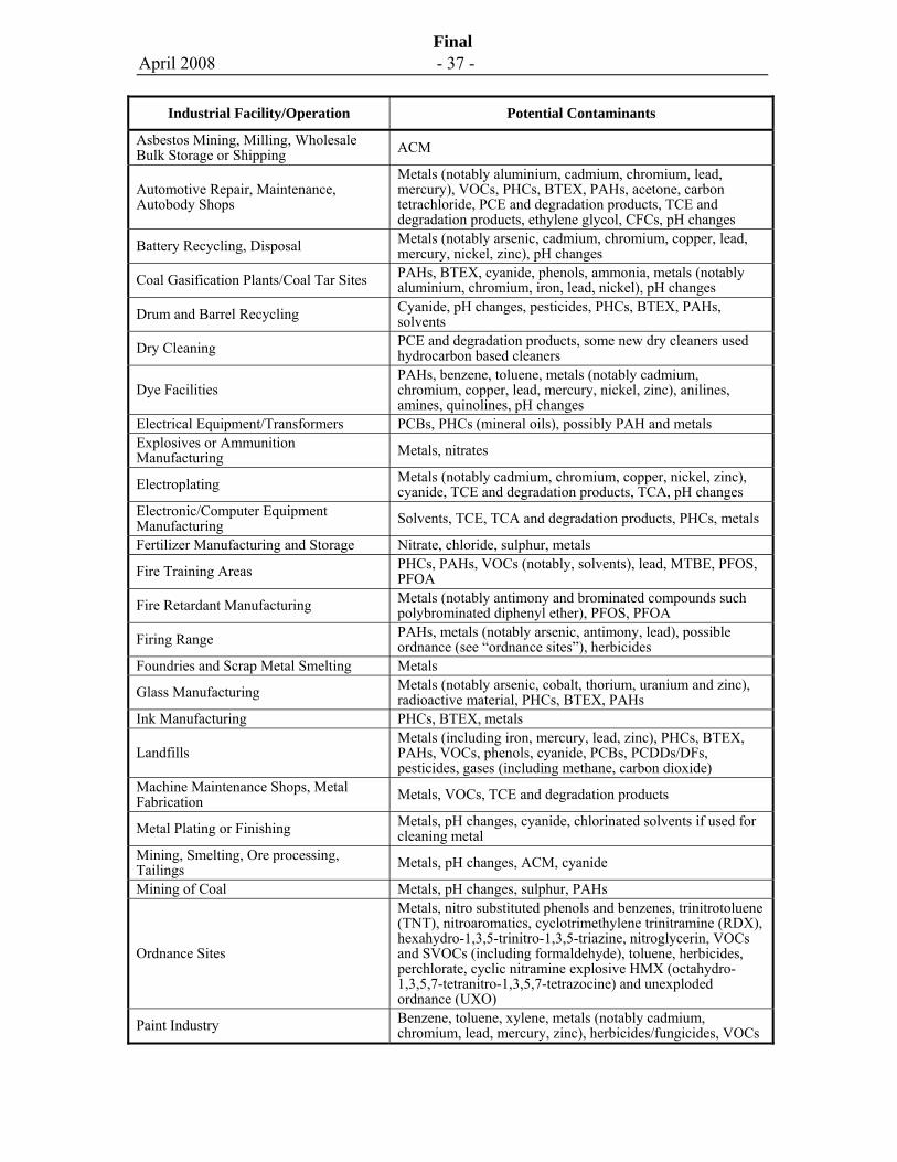
April 2008 - 37 -

Final

Industrial Facility/Operation Potential Contaminants

Asbestos Mining, Milling, Wholesale Bulk Storage or Shipping ACM

Automotive Repair, Maintenance, Autobody Shops

Metals (notably aluminium, cadmium, chromium, lead, mercury), VOCs, PHCs, BTEX, PAHs, acetone, carbon tetrachloride, PCE and degradation products, TCE and degradation products, ethylene glycol, CFCs, pH changes

Battery Recycling, Disposal Metals (notably arsenic, cadmium, chromium, copper, lead, mercury, nickel, zinc), pH changes

Coal Gasification Plants/Coal Tar Sites PAHs, BTEX, cyanide, phenols, ammonia, metals (notably aluminium, chromium, iron, lead, nickel), pH changes

Drum and Barrel Recycling Cyanide, pH changes, pesticides, PHCs, BTEX, PAHs, solvents

Dry Cleaning PCE and degradation products, some new dry cleaners used hydrocarbon based cleaners

Dye Facilities PAHs, benzene, toluene, metals (notably cadmium, chromium, copper, lead, mercury, nickel, zinc), anilines, amines, quinolines, pH changes

Electrical Equipment/Transformers PCBs, PHCs (mineral oils), possibly PAH and metals Explosives or Ammunition Manufacturing Metals, nitrates

Electroplating Metals (notably cadmium, chromium, copper, nickel, zinc), cyanide, TCE and degradation products, TCA, pH changes

Electronic/Computer Equipment Manufacturing Solvents, TCE, TCA and degradation products, PHCs, metals

Fertilizer Manufacturing and Storage Nitrate, chloride, sulphur, metals

Fire Training Areas PHCs, PAHs, VOCs (notably, solvents), lead, MTBE, PFOS, PFOA

Fire Retardant Manufacturing Metals (notably antimony and brominated compounds such polybrominated diphenyl ether), PFOS, PFOA

Firing Range PAHs, metals (notably arsenic, antimony, lead), possible ordnance (see “ordnance sites”), herbicides

Foundries and Scrap Metal Smelting Metals

Glass Manufacturing Metals (notably arsenic, cobalt, thorium, uranium and zinc), radioactive material, PHCs, BTEX, PAHs

Ink Manufacturing PHCs, BTEX, metals

Landfills Metals (including iron, mercury, lead, zinc), PHCs, BTEX, PAHs, VOCs, phenols, cyanide, PCBs, PCDDs/DFs, pesticides, gases (including methane, carbon dioxide)

Machine Maintenance Shops, Metal Fabrication Metals, VOCs, TCE and degradation products

Metal Plating or Finishing Metals, pH changes, cyanide, chlorinated solvents if used for cleaning metal

Mining, Smelting, Ore processing, Tailings Metals, pH changes, ACM, cyanide

Mining of Coal Metals, pH changes, sulphur, PAHs

Ordnance Sites

Metals, nitro substituted phenols and benzenes, trinitrotoluene (TNT), nitroaromatics, cyclotrimethylene trinitramine (RDX), hexahydro-1,3,5-trinitro-1,3,5-triazine, nitroglycerin, VOCs and SVOCs (including formaldehyde), toluene, herbicides, perchlorate, cyclic nitramine explosive HMX (octahydro-1,3,5,7-tetranitro-1,3,5,7-tetrazocine) and unexploded ordnance (UXO)

Paint Industry Benzene, toluene, xylene, metals (notably cadmium, chromium, lead, mercury, zinc), herbicides/fungicides, VOCs

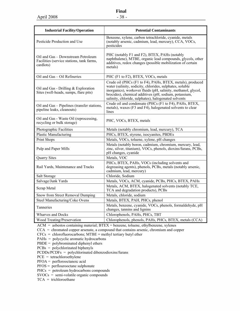
April 2008 - 38 -

Final

Industrial Facility/Operation Potential Contaminants

Pesticide Production and Use Benzene, xylene, carbon tetrachloride, cyanide, metals (notably arsenic, cadmium, lead, mercury), CCA, VOCs, pesticides

Oil and Gas – Downstream Petroleum Facilities (service stations, tank farms, cardlots)

PHC (notably F1 and F2), BTEX, PAHs (notably naphthalene), MTBE, organic lead compounds, glycols, other additives, redox changes (possible mobilization of certain metals)

Oil and Gas – Oil Refineries PHC (F1 to F2), BTEX, VOCs, metals

Oil and Gas - Drilling & Exploration Sites (well-heads, sumps, flare pits)

Crude oil (PHCs (F1 to F4), PAHs, BTEX, metals), produced water (salinity, sodicity, chlorides, sulphates, soluble inorganics), workover fluids (pH, salinity, methanol, glycol, brocides), chemical additives (pH, sodium, potassium, salinity, chloride, sulphates), halogenated solvents

Oil and Gas – Pipelines (transfer stations, pipeline leaks, cleanouts)

Crude oil and condensate (PHCs (F1 to F4), PAHs, BTEX, metals), waxes (F3 and F4), halogenated solvents to clear lines

Oil and Gas - Waste Oil (reprocessing, recycling or bulk storage) PHC, VOCs, BTEX, metals

Photographic Facilities Metals (notably chromium, lead, mercury), TCA Plastic Manufacturing PHCs, BTEX, styrene, isocyanites, PBDEs Print Shops Metals, VOCs, toluene, xylene, pH changes

Pulp and Paper Mills Metals (notably boron, cadmium, chromium, mercury, lead, zinc, silver, titanium), VOCs, phenols, dioxins/furans, PCBs, pH changes, cyanide

Quarry Sites Metals, VOC

Rail Yards, Maintenance and Tracks PHCs, BTEX, PAHs, VOCs (including solvents and degreasing agents), phenols, PCBs, metals (notably arsenic, cadmium, lead, mercury)

Salt Storage Chloride, Sodium Salvage/Junk Yards Metals, VOCs, ACM, cyanide, PCBs, PHCs, BTEX, PAHs

Scrap Metal Metals, ACM, BTEX, halogenated solvents (notably TCE, TCA and degradation products), PCBs

Snow from Street Removal Dumping Metals, chloride, sodium Steel Manufacturing/Coke Ovens Metals, BTEX, PAH, PHCs, phenol

Tanneries Metals, benzene, cyanide, VOCs, phenols, formaldehyde, pH changes, tannins and lignins

Wharves and Docks Chlorophenols, PAHs, PHCs, TBT Wood Treating/Preservation Chlorophenols, phenols, PAHs, PHCs, BTEX, metals (CCA) ACM = asbestos containing material; BTEX = benzene, toluene, ethylbenzene, xylenes CCA = chromated copper arsenate, a compound that contains arsenic, chromium and copper CFCs = chlorofluorocarbons; MTBE = methyl tertiary butyl ether PAHs = polycyclic aromatic hydrocarbons PBDE = polybrominated diphenyl ethers PCBs = polychlorinated biphenyls PCDDs/PCDFs = polychlorinated dibenzodioxins/furans PCE = tetrachloroethylene PFOA = perflorooctanoic acid PFOS = perflourooctane sulphonate PHCs = petroleum hydrocarbons compounds SVOCs = semi-volatile organic compounds TCA = trichloroethane

April 2008 - 39 -

Final

TCE = trichloroethylene UXO = unexploded ordnance VOCs = volatile organic compounds

4.1.4 Emergent or Less Common Chemicals

There are a number of emergent or less common chemicals in soil and/or groundwater that are receiving increased attention such as ammonium perchlorate, Chromium VI, nitrosodimethylamine (NDMA), 1,4-Dioxane, and 1,2,3-Trichloropropane (Exhibit 4-1). While information on the identification and significance of chemicals with no Canadian soil or groundwater guidelines may be limited, the site assessor should be aware that assessment of all chemicals of potential concern is warranted. Health Canada recommends that the proponent assess background concentrations, and review criteria from other jurisdictions. The proponent is also encouraged to contact the appropriate regulatory authority to discuss their proposed approach. Further evaluation of chemicals without regulatory guidelines, if present, would normally occur as part of a site specific risk assessment.

EXHIBIT 4-1: Less Common or Emergent Chemicals of Potential Concern

1,4-Dioxane: This chemical is used as a stabilizer for chlorinated solvents, particularly 1,1,1-trichloroethane. Releases of chlorinated solvents may be a primary source of 1,4-dioxane in the environment. It is a highly soluble chemical, and therefore mobile in groundwater.

Polybrominated Diphenyl Ether (PBDE): A family of flame-retardants used in a variety of products including computers, printers, cell phones, TVs, microwave appliances, upholstered furniture, plastic foam and carpeting. These chemicals have recently been detected in biosolids produced from sewage sludge (Gorgy et al., 2006).

Perchlorates: These chemicals are salts derived from perchloric acid (e.g., ammonium perchlorate). They occur both naturally and through manufacturing processes as an oxidizer in rocket fuel and component of fireworks, air-bags, and historic Chilean fertilizers. Most perchlorate salts are soluble in water, and therefore are highly mobile in groundwater.

N-nitrosodimethylamine (NDMA): One of several nitrosamines, NDMA is a by-product of the chlorination of wastewater, a by-product of the manufacture of pesticides, rubber tires, alkylamines and dyes, and a component of liquid rocket fuel (Environment Canada, 2002). It may be a chemical of potential concern where treated wastewater is used to recharge groundwater, although NDMA appears to biodegrade fairly readily in groundwater (Bradley et al., 2005).

Hexavalent Chromium (CrVI): This chemical is a heavy metal associated with industrial processes such as metal plating. It is also used as a corrosion inhibitor in

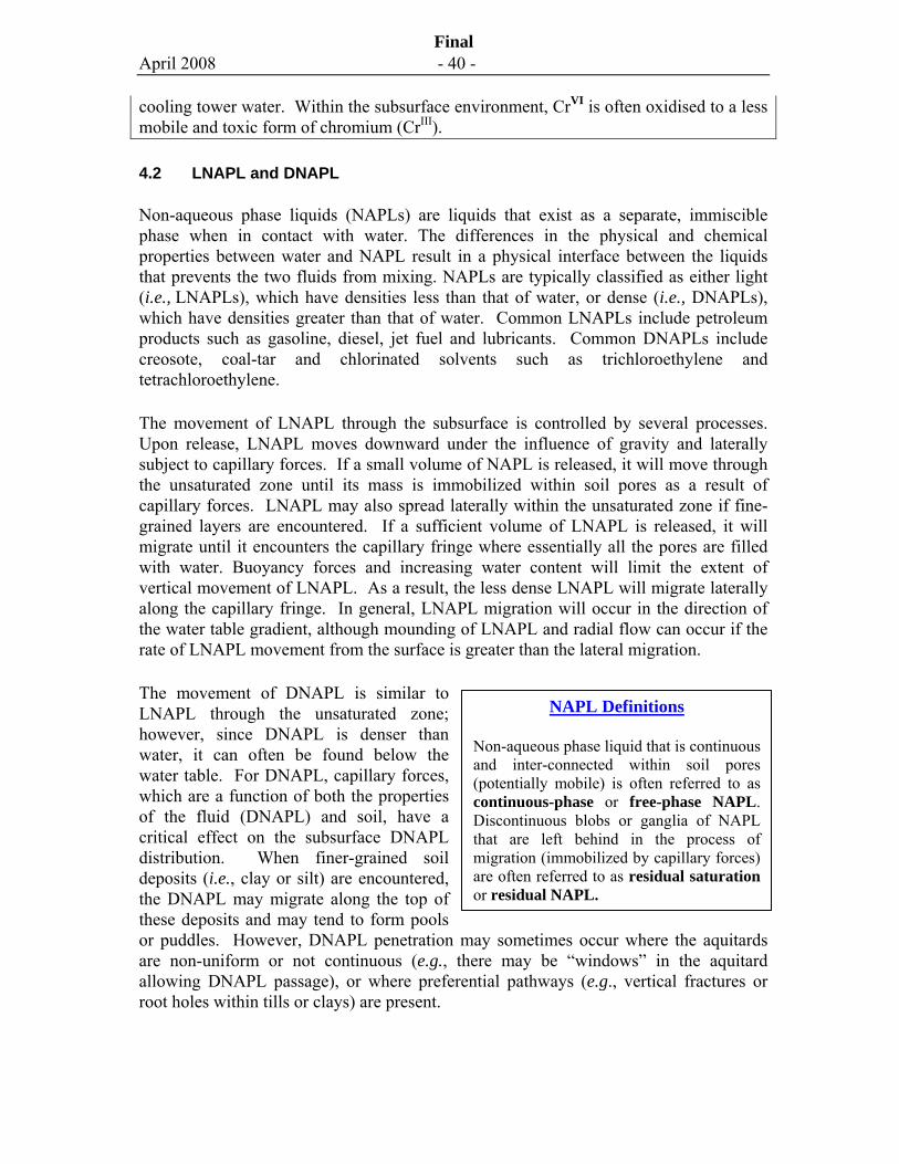
April 2008 - 40 -

Final

cooling tower water. Within the subsurface environment, CrVI is often oxidised to a less mobile and toxic form of chromium (CrIII).

4.2 LNAPL and DNAPL

Non-aqueous phase liquids (NAPLs) are liquids that exist as a separate, immiscible phase when in contact with water. The differences in the physical and chemical properties between water and NAPL result in a physical interface between the liquids that prevents the two fluids from mixing. NAPLs are typically classified as either light (i.e., LNAPLs), which have densities less than that of water, or dense (i.e., DNAPLs), which have densities greater than that of water. Common LNAPLs include petroleum products such as gasoline, diesel, jet fuel and lubricants. Common DNAPLs include creosote, coal-tar and chlorinated solvents such as trichloroethylene and tetrachloroethylene.

The movement of LNAPL through the subsurface is controlled by several processes. Upon release, LNAPL moves downward under the influence of gravity and laterally subject to capillary forces. If a small volume of NAPL is released, it will move through the unsaturated zone until its mass is immobilized within soil pores as a result of capillary forces. LNAPL may also spread laterally within the unsaturated zone if fine-grained layers are encountered. If a sufficient volume of LNAPL is released, it will migrate until it encounters the capillary fringe where essentially all the pores are filled with water. Buoyancy forces and increasing water content will limit the extent of vertical movement of LNAPL. As a result, the less dense LNAPL will migrate laterally along the capillary fringe. In general, LNAPL migration will occur in the direction of the water table gradient, although mounding of LNAPL and radial flow can occur if the rate of LNAPL movement from the surface is greater than the lateral migration.

The movement of DNAPL is similar to LNAPL through the unsaturated zone; however, since DNAPL is denser than water, it can often be found below the water table. For DNAPL, capillary forces, which are a function of both the properties of the fluid (DNAPL) and soil, have a critical effect on the subsurface DNAPL distribution. When finer-grained soil deposits (i.e., clay or silt) are encountered, the DNAPL may migrate along the top of these deposits and may tend to form pools or puddles. However, DNAPL penetration may sometimes occur where the aquitards are non-uniform or not continuous (e.g., there may be “windows” in the aquitard allowing DNAPL passage), or where preferential pathways (e.g., vertical fractures or root holes within tills or clays) are present.

NAPL Definitions

Non-aqueous phase liquid that is continuous and inter-connected within soil pores (potentially mobile) is often referred to as continuous-phase or free-phase NAPL. Discontinuous blobs or ganglia of NAPL that are left behind in the process of migration (immobilized by capillary forces) are often referred to as residual saturation or residual NAPL.

April 2008 - 41 -

Final

There are a number of key implications for LNAPL and DNAPL contamination that the site assessor should recognize. Both LNAPL and DNAPL zones are often long-term sources of dissolved contaminant plumes in groundwater, and often require delineation in order to address their remediation. While appropriate investigation techniques for both forms of contamination are essential, investigation for DNAPL is challenging since DNAPL source zones and migration pathways can be difficult to detect. For DNAPL, an indirect approach is often used to assess whether DNAPL may be present through comparison of dissolved chemical concentrations measured in a groundwater well to the theoretical solubility limit of the chemical. A commonly-adopted threshold for the possible presence of DNAPL is a dissolved concentration that exceeds 1 percent of its’ theoretical effective solubility (i.e., “1% rule-of-thumb”). Another key consideration is the stability of LNAPL or DNAPL zones. This, again, may be challenging to determine since their movement may be slow, and subtle changes in hydrogeological conditions may cause re-mobilization. A detailed evaluation of LNAPL mobility is provided in SABCS (2006a).

4.3 Groundwater Pathway

For evaluation of the groundwater pathway, the fate and transport processes along the transport pathway from contamination source to receptor should be understood. If there is contamination within the unsaturated zone, partitioning from the soil phase to aqueous phase will occur. Contaminants dissolved in soil-water will migrate in infiltrating water toward the water table. Below the water table, infiltrating water will migrate by advection, dispersion, and diffusion, mixing with flowing groundwater. Mixing will be enhanced by groundwater level fluctuations. The contaminant plume may “dive” as it migrates from the source area due to clean water recharge along the flowpath. Contaminants will migrate, to varying degrees, in the direction of groundwater flow and may come into contact with human receptors via use of well water or ecological receptors through discharge to surface water bodies.

An example of a conceptual site model for the groundwater pathway is shown in Figure 4-1. The following sections present an overview of fate and transport processes pertinent to this model.

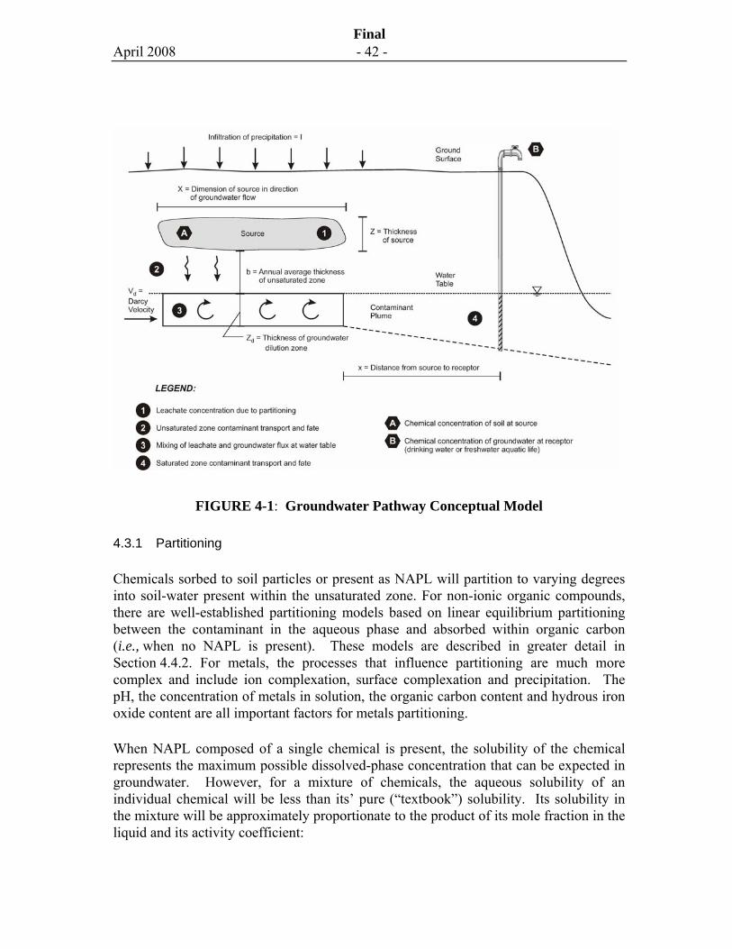
April 2008 - 42 -

Final

FIGURE 4-1: Groundwater Pathway Conceptual Model

4.3.1 Partitioning

Chemicals sorbed to soil particles or present as NAPL will partition to varying degrees into soil-water present within the unsaturated zone. For non-ionic organic compounds, there are well-established partitioning models based on linear equilibrium partitioning between the contaminant in the aqueous phase and absorbed within organic carbon (i.e., when no NAPL is present). These models are described in greater detail in Section 4.4.2. For metals, the processes that influence partitioning are much more complex and include ion complexation, surface complexation and precipitation. The pH, the concentration of metals in solution, the organic carbon content and hydrous iron oxide content are all important factors for metals partitioning.

When NAPL composed of a single chemical is present, the solubility of the chemical represents the maximum possible dissolved-phase concentration that can be expected in groundwater. However, for a mixture of chemicals, the aqueous solubility of an individual chemical will be less than its’ pure (“textbook”) solubility. Its solubility in the mixture will be approximately proportionate to the product of its mole fraction in the liquid and its activity coefficient:

April 2008 - 43 -

Final

Ciw = γi Xi Si [4.1]

where Ciw is the aqueous concentration (mg/L), γi is the activity coefficient (dimensionless), Xi is the mole fraction (dimensionless) and Si is the pure-chemical solubility (mg/L). In most cases, the activity coefficient can be assumed to be equal to unity for mixtures of organic chemicals. Corrections are required for chemicals such as naphthalene, which are normally solids, but exist as liquids in mixtures such as diesel and creosote (Schwarzenbach et al., 2003).

4.3.2 Unsaturated Zone Chemical Transport

The fate and transport of water-phase chemicals within the unsaturated zone (often termed the vadose zone) is dependent on numerous processes including advection, dispersion, diffusion, sorption, degradation or decay and volatilization. Advection is the bulk movement of water under a hydraulic head gradient, whereas diffusion is the process involving the transfer of chemicals from a higher to lower chemical potential by random molecular motion (Robinson and Stokes, 1959). The sorption of dissolved chemicals in soil-water to organic carbon or mineral surfaces will result in the retardation in the bulk movement of chemicals in soil-water.

For common organic chemicals such as benzene, toluene, ethylbenzene and xylenes, biodegradation has been demonstrated in groundwater under both aerobic and anaerobic conditions. Similar reaction kinetics would be expected in the unsaturated zone, except possibly for very dry conditions. Volatilization may be an important mechanism for mass loss for volatile chemicals in the vadose zone. Mechanical dispersion in the unsaturated zone has not been as extensively researched as saturated zone dispersion, although there are field-scale experiments where a longitudinal dispersivity of greater than 10 cm has been measured (Charbonneau and Daniel, 1993). Conceptually, transverse dispersion within the unsaturated zone could be highly variable depending on the potential for fingering or spreading based on horizontal layering of soil.

For unsaturated groundwater transport, the amount of water that infiltrates through the sub-surface (advection) has a direct impact on the quantity of chemical mass that is transported in the aqueous phase toward groundwater. The atmospheric and near-surface processes that influence infiltration may be characterized by a water balance model that describes the fundamental components of the surface hydrology for precipitation, snow melt, run-off, potential evaporation, actual soil evaporation, plant uptake and transpiration, changes in shallow soil moisture, and finally net infiltration or

Unsaturated Zone Hydraulic Conductivity

The prediction of soil-water movement through advection within the unsaturated zone is highly complex since the hydraulic conductivity is not constant (unlike the saturated zone) and instead is dependent on soil water (moisture) content in a non-linear manner. Within the unsaturated zone, the soil-water characteristic curve (SWCC) is vital to the prediction of soil properties such as unsaturated zone hydraulic conductivity. The theory and methods for prediction of unsaturated zone chemical transport are described in detail in SABCS (2006b).

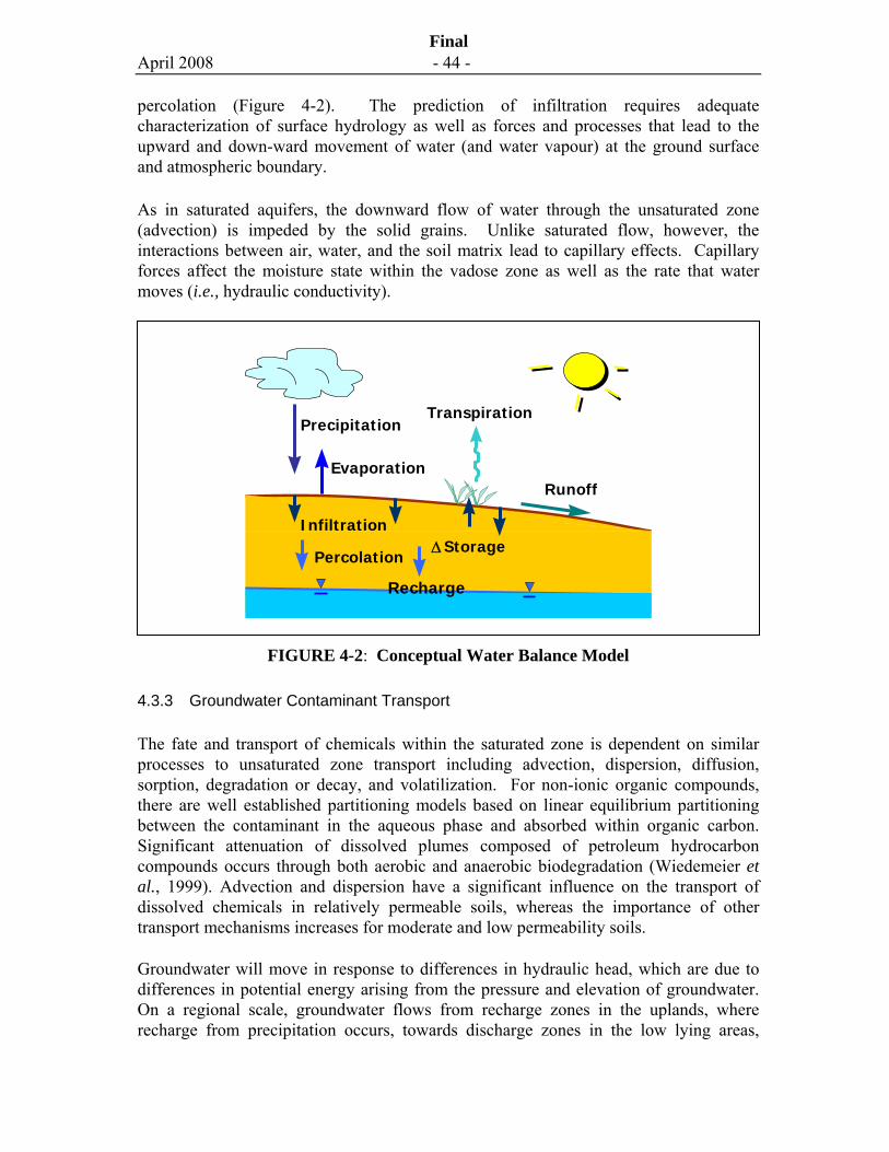
April 2008 - 44 -

Final

percolation (Figure 4-2). The prediction of infiltration requires adequate characterization of surface hydrology as well as forces and processes that lead to the upward and down-ward movement of water (and water vapour) at the ground surface and atmospheric boundary.

As in saturated aquifers, the downward flow of water through the unsaturated zone (advection) is impeded by the solid grains. Unlike saturated flow, however, the interactions between air, water, and the soil matrix lead to capillary effects. Capillary forces affect the moisture state within the vadose zone as well as the rate that water moves (i.e., hydraulic conductivity).

FIGURE 4-2: Conceptual Water Balance Model

4.3.3 Groundwater Contaminant Transport

The fate and transport of chemicals within the saturated zone is dependent on similar processes to unsaturated zone transport including advection, dispersion, diffusion, sorption, degradation or decay, and volatilization. For non-ionic organic compounds, there are well established partitioning models based on linear equilibrium partitioning between the contaminant in the aqueous phase and absorbed within organic carbon. Significant attenuation of dissolved plumes composed of petroleum hydrocarbon compounds occurs through both aerobic and anaerobic biodegradation (Wiedemeier et al., 1999). Advection and dispersion have a significant influence on the transport of dissolved chemicals in relatively permeable soils, whereas the importance of other transport mechanisms increases for moderate and low permeability soils.

Groundwater will move in response to differences in hydraulic head, which are due to differences in potential energy arising from the pressure and elevation of groundwater. On a regional scale, groundwater flows from recharge zones in the uplands, where recharge from precipitation occurs, towards discharge zones in the low lying areas,

Precipitation

RunoffEvaporation

Cover

Soil

Transpiration

Δ StorageInfiltration

Percolation

Recharge

April 2008 - 45 -

Final

forming springs and discharging to creeks, rivers, and lakes. In the discharge zones, hydraulic heads measured at depth can be above the ground surface, which results in flowing artesian conditions (i.e., the water level in the well rises above the ground surface and the well flows). On regional and local scales, groundwater flow occurs from the locations where the hydraulic head is high towards lower head regions, with energy loss along the flow line. The energy loss is proportional to the hydraulic conductivity (K), which is the ability of soil to transmit water and depends on the properties of both the soil and the fluid. The porosity, pore-size and pore continuity are important properties affecting hydraulic conductivity. Darcy’s Law governs the groundwater flow and is expressed as:

q = -K*dh/dl [4.2]

where q is the specific discharge [(L3/L2)/T] and dh (L) is the difference in hydraulic head over a distance dl (L). Specific discharge, or the volume of groundwater moving across a unit cross-sectional area, should not be confused with groundwater velocity v (L/T):

v = q/ne [4.3]

where ne is effective porosity (-) of the soil.

Hydraulic conductivity can vary over several orders-of-magnitude over relatively short distances in the subsurface. For example, in a hydrostratigraphic sequence where coarse sand unit pinches out against a silt unit, the change in hydraulic conductivity could be from 10-3 m/s in sand to 10-7 m/s in silt. As the groundwater velocity is proportional to hydraulic conductivity, this could result in a four orders-of-magnitude change in velocity between these units. In addition, the groundwater velocity typically varies within individual hydrostratigraphic units due to heterogeneity of subsurface media, although these changes are typically less than one order-of-magnitude.

Dispersion effectively results in the dilution of contamination during plume migration, and is usually of much greater significance in the longitudinal direction than in directions transverse to flow. The degree of dispersion is “scale-dependent,” meaning that the larger the region occupied by a contaminant plume, the larger will be the

Groundwater Flow Concepts Groundwater scientists have defined a number of useful hydrogeological concepts for purposes of understanding groundwater movement. There are two basic types of subsurface medium in which groundwater flows; porous media and fractured media. Porous media consist of aggregates of individual particles such as silt, sand or gravel. Fractured media can consist of soil (e.g., clay) or bedrock where groundwater moves primarily through fractures, cracks or other openings. Aquifers are defined as geologic deposits that are relatively permeable (sometimes defined on the basis of groundwater yield in economic quantities) whereas aquitards are relatively impermeable units. An unconfined aquifer is bounded by the water table while a confined aquifer lies beneath an aquitard.

April 2008 - 46 -

Final

significance of dispersion. Dispersion is also dependent on the heterogeneity of the aquifer. As a consequence of these factors, it is a relatively difficult variable to measure in the field, and is more commonly estimated based on empirical information obtained from the literature.

With the exception of chemicals such as chloride, which are not affected by sorption, dissolved chemicals in groundwater typically move through the subsurface at velocities that are less than the groundwater velocity. Contaminant velocity vc (L/T) is defined as:

vc = v / R [4.4]

where R is a retardation factor that accounts for the affects of sorption on the contaminant movement. For most contaminants, the retardation factor is higher for soils rich in organic matter than for mostly mineral soils. The organic matter content in soil samples is typically expressed as fraction of organic carbon foc (-).

4.3.4 Considerations for Fractured Bedrock

The properties of fractured bedrock can vary widely ranging from granitic bedrock with small fractures to limestone deposits where there are openings enlarged by dissolution, commonly referred to as karst deposits. In most bedrock aquifers, the groundwater migrates primarily through discontinuities (fractures and joints) in the rock matrix. Flow can also occur in the rock matrix in the presence of significant secondary porosity (e.g., in vuggy limestone). The groundwater velocity can be rapid and the influence of pumping may be seen over large areas, which has potential implications for well-head protection of groundwater drinking water supplies (Crowe et al., 2003).

Groundwater flow in fractured bedrock is complex and knowledge and techniques for characterizing groundwater flow and chemical transport in porous media cannot easily be applied to fractured rock. There are two basic approaches that have been traditionally used to conceptualise groundwater flow in fractured bedrock consisting of (i) the non-continuum approach (i.e., discrete fracture network or DFN) and (ii) the continuum approach (i.e., equivalent porous medium or EPM), as described in NRC (1996) and summarized below. DFN models may be applied when individual fractures or groups of fractures significantly influence groundwater flow and solute transport. The modeling of flow and transport through a DFN approach is highly complex and assumes that fluid flow can be predicted from knowledge of the fracture geometry and data on the hydraulic properties of individual fractures. As there is always uncertainty in geometry and properties of fracture networks, DFN models relay heavily on statistical concepts for predictions. Under the EPM approach, the individual fractures are not explicitly treated in the model. Instead, at the scale of interest, hydraulic properties represent the volume-averaged behaviour of many fractures. Similar concepts as applied to porous media may be used to model contaminant transport under the EPM, but these predictions are only valid if it is possible to define a reasonable averaging volume.

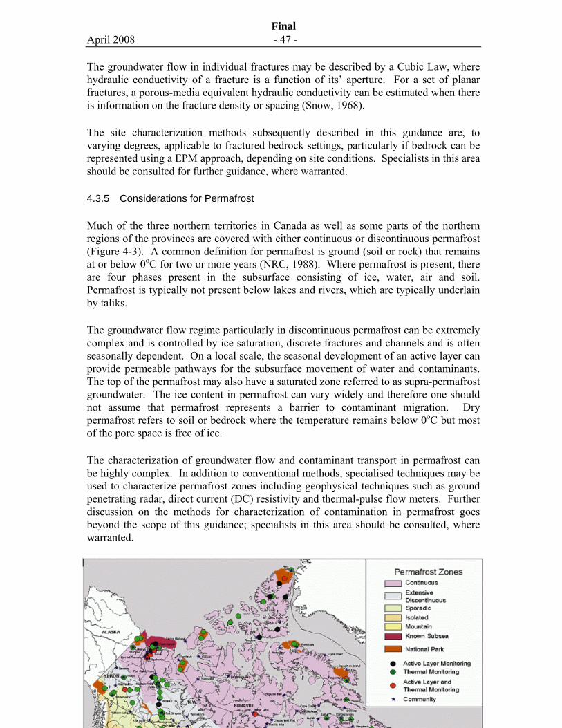
April 2008 - 47 -

Final

The groundwater flow in individual fractures may be described by a Cubic Law, where hydraulic conductivity of a fracture is a function of its’ aperture. For a set of planar fractures, a porous-media equivalent hydraulic conductivity can be estimated when there is information on the fracture density or spacing (Snow, 1968).

The site characterization methods subsequently described in this guidance are, to varying degrees, applicable to fractured bedrock settings, particularly if bedrock can be represented using a EPM approach, depending on site conditions. Specialists in this area should be consulted for further guidance, where warranted.

4.3.5 Considerations for Permafrost

Much of the three northern territories in Canada as well as some parts of the northern regions of the provinces are covered with either continuous or discontinuous permafrost (Figure 4-3). A common definition for permafrost is ground (soil or rock) that remains at or below 0oC for two or more years (NRC, 1988). Where permafrost is present, there are four phases present in the subsurface consisting of ice, water, air and soil. Permafrost is typically not present below lakes and rivers, which are typically underlain by taliks.

The groundwater flow regime particularly in discontinuous permafrost can be extremely complex and is controlled by ice saturation, discrete fractures and channels and is often seasonally dependent. On a local scale, the seasonal development of an active layer can provide permeable pathways for the subsurface movement of water and contaminants. The top of the permafrost may also have a saturated zone referred to as supra-permafrost groundwater. The ice content in permafrost can vary widely and therefore one should not assume that permafrost represents a barrier to contaminant migration. Dry permafrost refers to soil or bedrock where the temperature remains below 0oC but most of the pore space is free of ice.

The characterization of groundwater flow and contaminant transport in permafrost can be highly complex. In addition to conventional methods, specialised techniques may be used to characterize permafrost zones including geophysical techniques such as ground penetrating radar, direct current (DC) resistivity and thermal-pulse flow meters. Further discussion on the methods for characterization of contamination in permafrost goes beyond the scope of this guidance; specialists in this area should be consulted, where warranted.

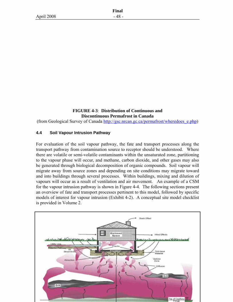
April 2008 - 48 -

Final

FIGURE 4-3: Distribution of Continuous and

Discontinuous Permafrost in Canada (from Geological Survey of Canada http://gsc.nrcan.gc.ca/permafrost/wheredoes_e.php)

4.4 Soil Vapour Intrusion Pathway

For evaluation of the soil vapour pathway, the fate and transport processes along the transport pathway from contamination source to receptor should be understood. Where there are volatile or semi-volatile contaminants within the unsaturated zone, partitioning to the vapour phase will occur, and methane, carbon dioxide, and other gases may also be generated through biological decomposition of organic compounds. Soil vapour will migrate away from source zones and depending on site conditions may migrate toward and into buildings through several processes. Within buildings, mixing and dilution of vapours will occur as a result of ventilation and air movement. An example of a CSM for the vapour intrusion pathway is shown in Figure 4-4. The following sections present an overview of fate and transport processes pertinent to this model, followed by specific models of interest for vapour intrusion (Exhibit 4-2). A conceptual site model checklist is provided in Volume 2.

April 2008 - 49 -

Final

FIGURE 4-4: Example of a Conceptual Site Model for Vapour Intrusion

into a Residential Building (from USEPA, 2002)

4.4.1 Contamination Sources

Common contaminants of potential concern for soil vapour intrusion comprise a range of organic chemicals including petroleum hydrocarbons from fuel products, coal-tar or creosote, and chlorinated solvents.

Petroleum hydrocarbons are associated with fuels such as gasoline, jet fuel and diesel and are mixtures of hundreds of compounds. While often the focus of risk assessments are benzene, toluene, ethylbenzene and xylenes (BTEX), and polycyclic aromatic hydrocarbons (PAHs) these compounds only represent a small fraction of hydrocarbon vapours and there may be other specific compounds of interest such as hexane, decane, trimethylbenzenes and naphthalene, depending on the fuel type. Typically, analytical tests for hydrocarbon vapours will also include hydrocarbon fractions based on carbon chain length (e.g., F1 and F2 as defined in CCME (2008)) and aromatic and aliphatic fractions.

Coal-tar, associated with former manufactured gas plants (MGP), and creosote, associated with wood preservation, have similar organic contaminants of potential concern composed of monocyclic aromatic hydrocarbons, such as BTEX, and PAHs. There is significant variation in the volatility and mobility of PAH compounds ranging from naphthalene, considered a semi-volatile, to five- and six-ring PAHs, which are essentially non-volatile. While some of the heavier PAH compounds are identified as COPCs for the vapour intrusion pathway based on conservative screening approaches (e.g., Health Canada and USEPA vapour intrusion guidance), their vapour concentrations are relatively low and organic carbon partitioning coefficients (Koc) tend to be higher. As a consequence, the mobility of heavier molecular weight PAHs via soil vapour transport is limited and, for practical purposes, is not of potential concern for vapour intrusion. Similar considerations apply to other heavier molecular weight organic chemicals with similar properties.

April 2008 - 50 -

Final

Common chlorinated solvents include tetrachloroethylene or perchloroethylene (PCE), trichloroethylene (TCE) and 1,1,1-trichloroethane (TCA), and associated breakdown products of biodegradation or abiotic transformation (e.g., cis- and trans-1,2-dichloroethylene (cis-1,2-DCE), 1,1-dichloroethylene (1,1-DCE) and vinyl chloride). Most chlorinated solvents are relatively mobile and persistent within the unsaturated zone due to their relatively low solubility, high volatility and their resistance to degradation under aerobic conditions.

Inorganic chemicals such as mercury may also pose a potential vapour inhalation risk since elemental mercury has a high vapour pressure.

Soil gases such as methane, carbon dioxide and, in some cases, hydrogen sulphide, may be generated as a by-product of the anaerobic decomposition of organic chemicals such as petroleum fuels, waste material (e.g., refuse) and/or native organic matter (e.g., peat). The presence of these gases may represent a potential safety hazard through explosion or asphyxiation. Methane is explosive in the range of 5 to 15 percent by volume in air. Gas produced by microbiological activity may generate pressure gradients that enhance subsurface vapour migration through advection. Another source of pressure-driven gas is leaking natural gas lines. The CSM subsequently described in this chapter does not address assessment of sites where there is potential for significant pressure-driven gas flow.

4.4.2 Chemical Transfer to Vapour Phase (Volatilization)

Chemical transfer to the vapour phase may occur through partitioning of NAPL present above the water table into soil gas (“vapourisation”) or partitioning of dissolved chemicals in soil-water above the water table into soil gas (“volatilization”). The NAPL is referred to as a primary source of vapours while a dissolved phase plume is referred to as a secondary source. Soil contamination within the unsaturated zone also represents a potential source of vapours.

The distribution of NAPL relative to the water table will have a large influence on its potential to volatilise and migrate to indoor air. If the NAPL is situated below the water table, then volatilisation will be relatively limited since, as subsequently discussed in this chapter, the mass transport through groundwater is relatively slow due to the low diffusion rate in water, and since vertical dispersion tends to be limited.

For a secondary source where chemicals are present only as a dissolved phase in groundwater, their distribution below the water table will also determine their potential to volatilize. If volatile chemicals are present near the surface of the water table, volatilization will readily occur. In contrast, if there is a layer of “clean” groundwater above contaminated water, then the rate of volatilization will decrease.

Equilibrium partitioning models are typically used to estimate the distribution of chemicals between different phases. Where NAPL is present above the water table, a

April 2008 - 51 -

Final

two-phase model based on the vapour pressure of the chemical is used to estimate the soil vapour concentration. Raoult’s Law is used to account for partitioning for a multi-component mixture of chemicals, which is a function of the mole fraction and vapour pressure, as follows:

Cv = 1000 * MW * X * VP / (R * T) [4-5]

where Cv is the soil vapour concentration (mg/m3), MW is the molecular weight (g/mole), X is the mole fraction (dimensionless), VP is the vapour pressure (atm), R is the gas constant (m3-atm/K-mole), and T is the temperature (K).

For dissolved chemicals in groundwater, the Henry’s Law constant is typically used to estimate the vapour concentration in equilibrium with water, as follows:

Cv = 1000 * Cg * H’ [4-6]

where Cg is the groundwater concentration (mg/L) and H’ is the dimensionless Henry’s Law constant. Since it is not possible to obtain a soil gas sample at the water table (i.e., due to the capillary transition zone), the measured soil vapour concentration should be lower than that predicted using the Henry’s Law constant. This is because there will be attenuation of chemical concentrations by diffusion (and possibly biodegradation) within the capillary fringe and transition zone between the water table and region where there are continuous gas-filled soil pores. The attenuation within the capillary zone has implications for soil vapour intrusion modeling and comparison of measured and predicted soil vapour concentrations.

Where there is soil contamination, but no NAPL, a three phase model1 for partitioning between sorbed, aqueous, and vapour phases can be used to estimate the soil vapour concentration, as follows:

Ct = Cw (Kd + (θw + θa*H’/ρb)) Kd = Koc * foc [4-7]

where Ct is the total soil concentration (mg/kg), Cw is the soil-water concentration (mg/L), Koc is the organic carbon-water partition coefficient (L/kg), foc is the fraction organic carbon (dimensionless), θw is the water-filled porosity (dimensionless), θa is the air-filled porosity (dimensionless), H’ is the Henry’s Law constant (dimensionless) and ρb is the bulk dry density (kg/L). If, under equilibrium, the three phases become saturated by the chemical, then the remainder of the chemical will be in its pure form (i.e., NAPL). Guidance on calculation of the soil saturation (“Csat”) concentration for NAPL is provided in USEPA (1996).

1 A four-phase model for partitioning between the sorbed, aqueous, soil-air and NAPL phases has been developed and

applied to the vapour intrusion pathway (Park and San Juan, 2000). The four-phase model better accounts for mass and volume conservation between all four phases and may enable more accurate estimation of mole fraction in the NAPL phase, for a multi-component mixture.

April 2008 - 52 -

Final

For non-ionizing organic chemicals, a linear equilibrium partitioning model is widely used to predict absorption of organics into native organic carbon. Studies have shown that the sorption of organics by soils is highly correlated with the foc (e.g., Chiou et al., 1979; Hassett et al., 1980; Hassett and Banwart. 1989), provided the foc is above a critical level. USEPA (1996) suggests that when foc is below about 0.001, adsorption to inorganic mineral surfaces becomes important. While soil partitioning models are well established, the accuracy of such models to predict soil vapour concentrations is poor. Therefore, it is generally not good practise to try to estimate soil vapour concentrations from soil concentration data. Instead, they should be predicted from groundwater data using Henry’s Law constant (when appropriate) or directly measured.

4.4.3 Vadose Zone Fate and Transport Processes

Fate and transport processes in the vadose zone that influence the movement of chemicals from a contamination source toward a building include: diffusion; advection; dispersion; partitioning between soil, water and gas phases; and, biodegradation reactions. Several of the fate and transport processes that influence soil vapour intrusion are conceptually shown in Figure 4-4. In this example, volatilization is occurring just above the top of the capillary fringe to create soil vapours. These vapours are subsequently transported upwards toward the ground surface via diffusion. Closer to the building, if the building is depressurized relative to atmospheric pressure, advective soil gas transport may be the dominant process. The rate of volatilization at the contamination source is controlled by the mass flux rate for chemical migration away from the source. This will vary temporally as a result of fluctuations in various factors such as moisture content, temperature and elevation of the water table.

Diffusion

Diffusion is the movement of molecules from an area of higher concentration to an area of lower concentration, as influenced by their kinetic energy. The rate that a chemical will diffuse is a function of the concentration difference, or gradient, and the compound- and temperature-dependent diffusion coefficient. The mass flux, J (M/L2-T), is calculated by Fick’s Law, as follows:

J = -Deff * δC / δZ [4.8]

Where Deff is the effective diffusion coefficient (L2/T), C is the vapour concentration (mass/volume of gas) and z is the distance over which the concentration change is measured (L). The diffusive flux is less in soil than in a gas-filled volume as a result of the tortuosity or non-linear migration path for diffusing gas species. Mathematically, this is expressed as the effective diffusion coefficient, typically estimated from the Millington-Quirk relationship (1961):

Deff = Da * θa 3.33. / θ 2 + Dw/H’ * θw 3.33. / θ 2 [4-9]

April 2008 - 53 -

Final

Diffusion coefficients in air (Da, L2/T) are about four orders-of-magnitude higher than in water (Dw, L2/T); therefore, diffusion is much faster through the air-filled soil pores, than through water-filled soil pores, and the second term in equation 4-9 tends not be important except under nearly saturated conditions or for compounds with very low Henry’s Law constant (i.e., dimensionless H’ less than 0.001). When contamination is limited to dissolved chemicals in groundwater, diffusion through the capillary fringe is often the rate-limiting process because the moisture content in the capillary fringe is high, and may even be completely saturated. The thickness of the capillary fringe increases with decreasing soil grain size. Diffusion rates may also be highly sensitive to the presence of fine-grained, high moisture content soil layers within the vadose zone. There may also be a “rain-shadow” below a building with locally drier soils beneath the building (although drains and gutters may influence the soil moisture distribution).

Sorption

As soil vapours migrate away from contamination source zones, the transport of soil vapours will be retarded due to sorption to the soil matrix and transfer of chemicals into soil water. Soils with higher native organic carbon will tend to have a greater sorption capacity. While partitioning into soil water will occur rapidly, for some chemicals biodegradation may occur simultaneously to reduce the concentration in soil water. This allows for the continuous partitioning of the chemical into the soil water, thus reducing the concentration in the vapour phase.

Biodegradation

Different organic compounds will biodegrade at different rates, and with various oxygen demands. For example, the aerobic biodegradation of volatile petroleum hydrocarbons in the vadose zone (e.g., BTEX) has been demonstrated through several investigations (Ostendorf and Campbell, 1991; Ririe et al., 1998; Roggemans et al., 2002; Hers et al., 2000; Hers et al., 2002). Several of these studies indicate orders-of-magnitude bioattenuation of hydrocarbon vapour concentrations over relatively small distances within the vadose zone. Since chlorinated solvents such as PCE and TCE degrade primarily under anaerobic conditions through reductive dechlorination (Wiedemeier et al., 1999), biotransformation of these compounds will usually be limited due to the presence of oxygen within the unsaturated zone. There is evidence of aerobic biodegradation of vinyl chloride.

Vadose Zone Advection

Gas-phase advective transport can occur as a result of fluctuations in atmospheric pressure (e.g., barometric pumping), water movement, water table fluctuations, and density gradients due to composition and temperature variations (soil gas advection due to building depressurization is discussed in Section 4.4.4). For most geologic environments, diffusion is the dominant vadose zone transport process; however, soil gas advection can be important where there are high permeability, relatively deep unsaturated zone deposits (i.e., tens of metres deep) and/or methanogenesis is

April 2008 - 54 -

Final

significant. Choi and Smith (2005) through a modeling study found that pressure-driven advective flux increased for deep, drier, permeable deposits; nevertheless, for all combinations of scenarios, the diffusive flux was at least one order-of-magnitude greater than the advective flux. Where there are relatively high soil gas advection rates, dispersion may also be important. Dispersion is a mixing process that is caused by small-scale variations in air velocities in soil. The effects of these velocity variations are similar to the effects of diffusion (Auer, 1996).

4.4.4 Near-Building Processes for Soil Vapour Intrusion

The primary process for soil vapour intrusion into buildings is typically soil gas advection, although vapour migration will also occur as a result of diffusion through the building foundation. Model sensitivity analyses suggest that soil gas advection will be the dominant mechanism when the building depressurization (relative to ambient air) is greater than about 1 Pascal (Hers et al., 2003; Johnson, 2005), which will be exceeded at many residential buildings.

Soil gas advection can occur through untrapped floor drains, edge cracks at the building wall and floor slab interface (shown in Figure 4-4), unsealed entry points for utilities, expansion joints and other cracks and openings, if present. Field research programs that include pressure data for soil adjacent to the residential building foundation indicate that most of the soil gas flow occurs within 1 to 2 m of the foundation (Garbesi et al, 1993; Hers et al., 2002). Therefore, the properties of the backfill surrounding the foundation are important, as well as any nearby utility corridors. Field measurements and model simulations indicate that for most sites, the permeability of soil near the building will control the rate of soil gas flow, as opposed to the permeability of the building foundation.

Depressurization of the building airspace relative to the ambient (outdoor) air pressure can be caused by a number of factors including temperature differences between indoor and outdoor air (i.e., “stack effect”), wind-loading and operation of the building heating, ventilation and air-conditioning (HVAC) systems. The operation of HVAC systems can cause a building to be depressurized through insufficient combustion air for furnaces or unbalanced heating and ventilation systems where the exhaust air flow rate exceeds the intake flow rate. Commercial buildings may be either positively or negatively pressurized depending on HVAC system design, operation and environmental conditions. Diffusion through the building foundation will readily occur through cracks and openings in the foundation. Diffusion rates through intact building materials are relatively low, but will depend somewhat on material type (e.g., poured concrete slab, concrete block wall). Plastic moisture vapour barriers placed during the construction of slabs may reduce diffusion to some degree, but will have little effect on reducing advection, since significant soil gas flows can occur through small openings.

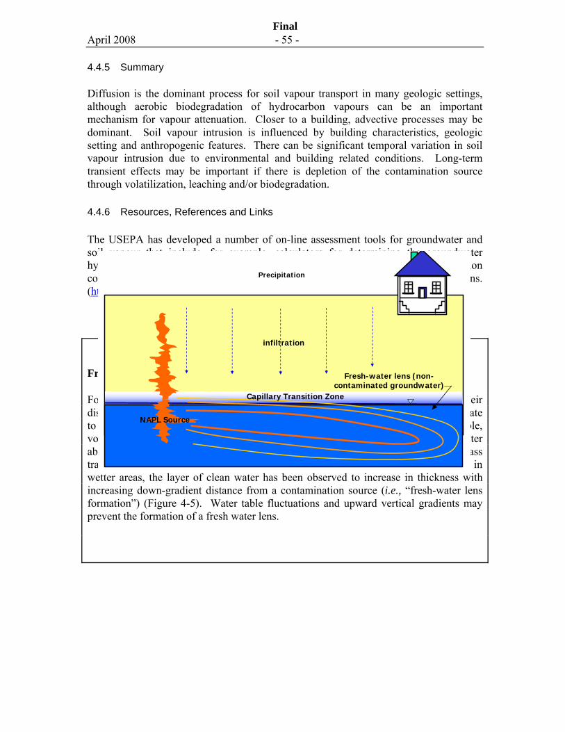
April 2008 - 55 -

Final

4.4.5 Summary

Diffusion is the dominant process for soil vapour transport in many geologic settings, although aerobic biodegradation of hydrocarbon vapours can be an important mechanism for vapour attenuation. Closer to a building, advective processes may be dominant. Soil vapour intrusion is influenced by building characteristics, geologic setting and anthropogenic features. There can be significant temporal variation in soil vapour intrusion due to environmental and building related conditions. Long-term transient effects may be important if there is depletion of the contamination source through volatilization, leaching and/or biodegradation.

4.4.6 Resources, References and Links

The USEPA has developed a number of on-line assessment tools for groundwater and soil vapour that include, for example, calculators for determining the groundwater hydraulic gradient, retardation factors for solute transport, plume diving, diffusion coefficients, Johnson and Ettinger alpha calculator and unit conversions. (http://www.epa.gov/athens/onsite/)

EXHIBIT 4-2: Conceptual Site Scenarios for Vapour Intrusion

Fresh-Water Lens

For chemicals present only in groundwater (i.e., dissolved phase sources), their distribution below the water table will determine their potential to volatilize and migrate to indoor air. If volatile chemicals are present near the surface of the water table, volatilization will readily occur. In contrast, if there is a layer of “clean” groundwater above contaminated water, then the rate of volatilization will decrease since mass transport is controlled by diffusion and dispersion in groundwater. At some sites in wetter areas, the layer of clean water has been observed to increase in thickness with increasing down-gradient distance from a contamination source (i.e., “fresh-water lens formation”) (Figure 4-5). Water table fluctuations and upward vertical gradients may prevent the formation of a fresh water lens.

Fresh-water lens (non-contaminated groundwater)

infiltration

Precipitation

Capillary Transition Zone

NAPL Source

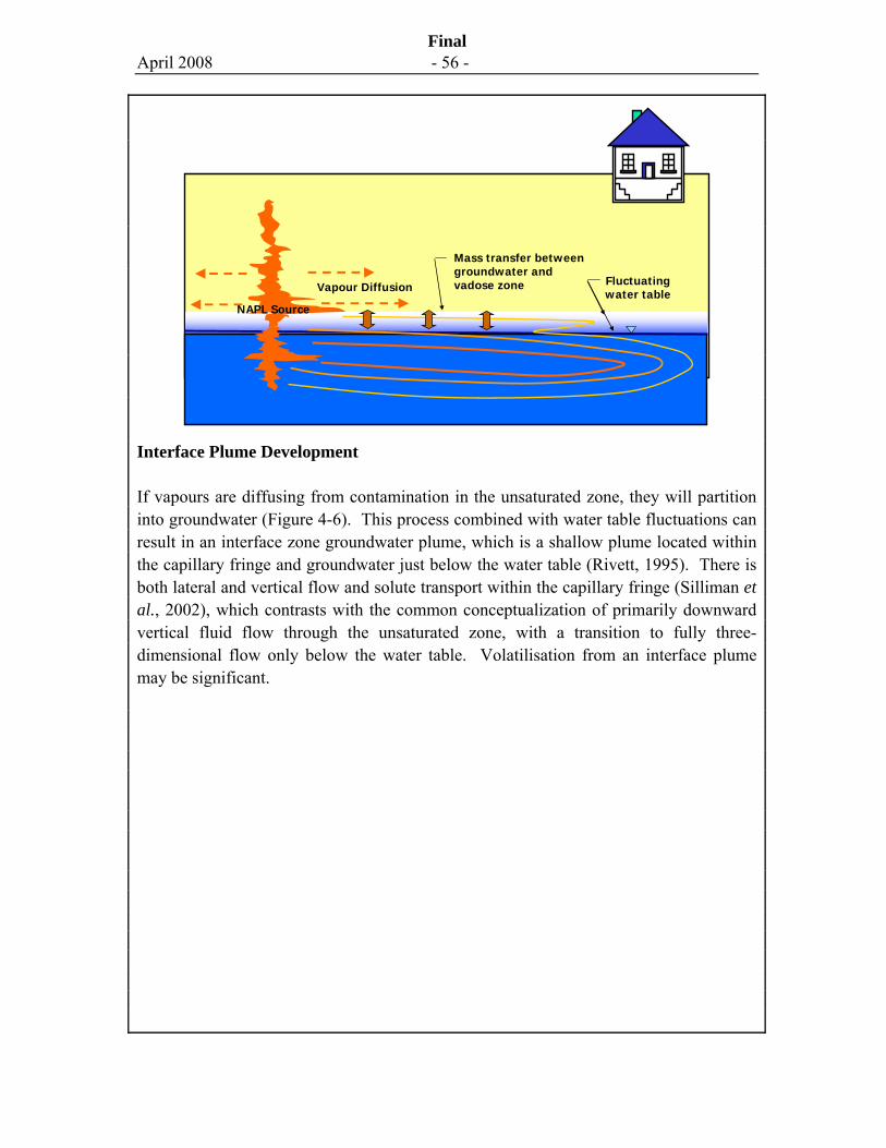
April 2008 - 56 -

Final

FIGURE 4-5. Fresh Water Lens

Interface Plume Development

If vapours are diffusing from contamination in the unsaturated zone, they will partition into groundwater (Figure 4-6). This process combined with water table fluctuations can result in an interface zone groundwater plume, which is a shallow plume located within the capillary fringe and groundwater just below the water table (Rivett, 1995). There is both lateral and vertical flow and solute transport within the capillary fringe (Silliman et al., 2002), which contrasts with the common conceptualization of primarily downward vertical fluid flow through the unsaturated zone, with a transition to fully three-dimensional flow only below the water table. Volatilisation from an interface plume may be significant.

Vapour Diffusion Fluctuatingwater table

Mass transfer between groundwater andvadose zone

NAPL Source

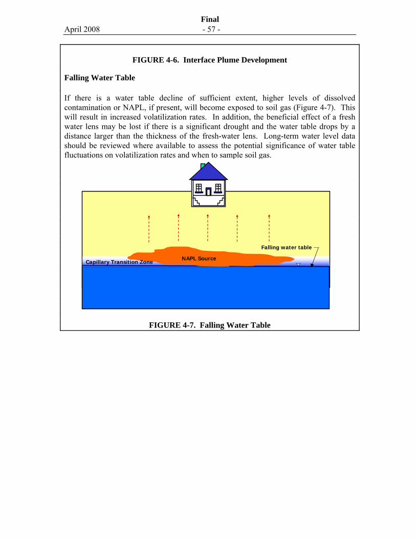
April 2008 - 57 -

Final

FIGURE 4-6. Interface Plume Development

Falling Water Table

If there is a water table decline of sufficient extent, higher levels of dissolved contamination or NAPL, if present, will become exposed to soil gas (Figure 4-7). This will result in increased volatilization rates. In addition, the beneficial effect of a fresh water lens may be lost if there is a significant drought and the water table drops by a distance larger than the thickness of the fresh-water lens. Long-term water level data should be reviewed where available to assess the potential significance of water table fluctuations on volatilization rates and when to sample soil gas.

FIGURE 4-7. Falling Water Table

Falling water table

Capillary Transition ZoneNAPL Source

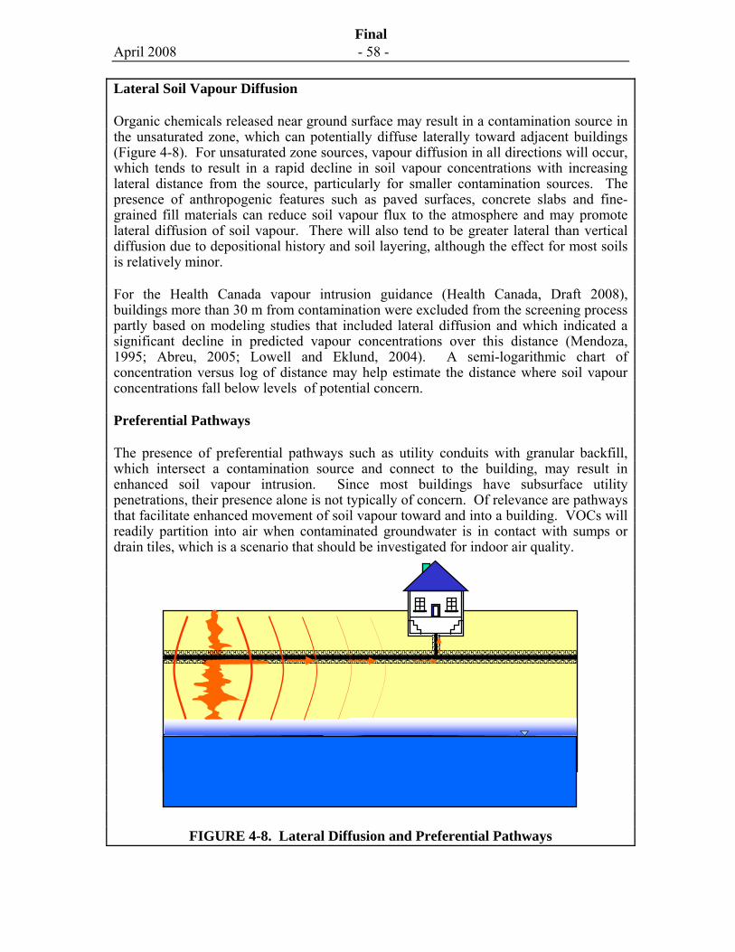
April 2008 - 58 -

Final

Lateral Soil Vapour Diffusion

Organic chemicals released near ground surface may result in a contamination source in the unsaturated zone, which can potentially diffuse laterally toward adjacent buildings (Figure 4-8). For unsaturated zone sources, vapour diffusion in all directions will occur, which tends to result in a rapid decline in soil vapour concentrations with increasing lateral distance from the source, particularly for smaller contamination sources. The presence of anthropogenic features such as paved surfaces, concrete slabs and fine-grained fill materials can reduce soil vapour flux to the atmosphere and may promote lateral diffusion of soil vapour. There will also tend to be greater lateral than vertical diffusion due to depositional history and soil layering, although the effect for most soils is relatively minor.

For the Health Canada vapour intrusion guidance (Health Canada, Draft 2008), buildings more than 30 m from contamination were excluded from the screening process partly based on modeling studies that included lateral diffusion and which indicated a significant decline in predicted vapour concentrations over this distance (Mendoza, 1995; Abreu, 2005; Lowell and Eklund, 2004). A semi-logarithmic chart of concentration versus log of distance may help estimate the distance where soil vapour concentrations fall below levels of potential concern.

Preferential Pathways

The presence of preferential pathways such as utility conduits with granular backfill, which intersect a contamination source and connect to the building, may result in enhanced soil vapour intrusion. Since most buildings have subsurface utility penetrations, their presence alone is not typically of concern. Of relevance are pathways that facilitate enhanced movement of soil vapour toward and into a building. VOCs will readily partition into air when contaminated groundwater is in contact with sumps or drain tiles, which is a scenario that should be investigated for indoor air quality.

FIGURE 4-8. Lateral Diffusion and Preferential Pathways

Capillary Transition ZoneNAPL Source

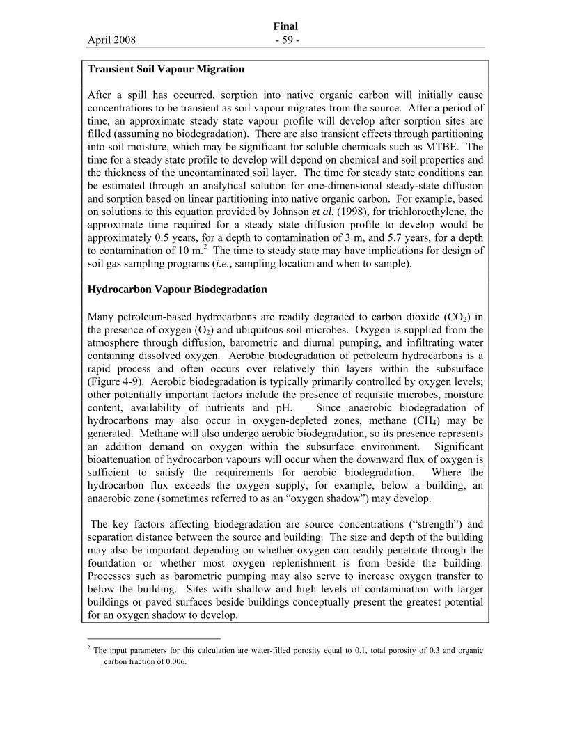
April 2008 - 59 -

Final

Transient Soil Vapour Migration After a spill has occurred, sorption into native organic carbon will initially cause concentrations to be transient as soil vapour migrates from the source. After a period of time, an approximate steady state vapour profile will develop after sorption sites are filled (assuming no biodegradation). There are also transient effects through partitioning into soil moisture, which may be significant for soluble chemicals such as MTBE. The time for a steady state profile to develop will depend on chemical and soil properties and the thickness of the uncontaminated soil layer. The time for steady state conditions can be estimated through an analytical solution for one-dimensional steady-state diffusion and sorption based on linear partitioning into native organic carbon. For example, based on solutions to this equation provided by Johnson et al. (1998), for trichloroethylene, the approximate time required for a steady state diffusion profile to develop would be approximately 0.5 years, for a depth to contamination of 3 m, and 5.7 years, for a depth to contamination of 10 m.2 The time to steady state may have implications for design of soil gas sampling programs (i.e., sampling location and when to sample). Hydrocarbon Vapour Biodegradation

Many petroleum-based hydrocarbons are readily degraded to carbon dioxide (CO2) in the presence of oxygen (O2) and ubiquitous soil microbes. Oxygen is supplied from the atmosphere through diffusion, barometric and diurnal pumping, and infiltrating water containing dissolved oxygen. Aerobic biodegradation of petroleum hydrocarbons is a rapid process and often occurs over relatively thin layers within the subsurface (Figure 4-9). Aerobic biodegradation is typically primarily controlled by oxygen levels; other potentially important factors include the presence of requisite microbes, moisture content, availability of nutrients and pH. Since anaerobic biodegradation of hydrocarbons may also occur in oxygen-depleted zones, methane (CH4) may be generated. Methane will also undergo aerobic biodegradation, so its presence represents an addition demand on oxygen within the subsurface environment. Significant bioattenuation of hydrocarbon vapours will occur when the downward flux of oxygen is sufficient to satisfy the requirements for aerobic biodegradation. Where the hydrocarbon flux exceeds the oxygen supply, for example, below a building, an anaerobic zone (sometimes referred to as an “oxygen shadow”) may develop. The key factors affecting biodegradation are source concentrations (“strength”) and separation distance between the source and building. The size and depth of the building may also be important depending on whether oxygen can readily penetrate through the foundation or whether most oxygen replenishment is from beside the building. Processes such as barometric pumping may also serve to increase oxygen transfer to below the building. Sites with shallow and high levels of contamination with larger buildings or paved surfaces beside buildings conceptually present the greatest potential for an oxygen shadow to develop.

2 The input parameters for this calculation are water-filled porosity equal to 0.1, total porosity of 0.3 and organic

carbon fraction of 0.006.

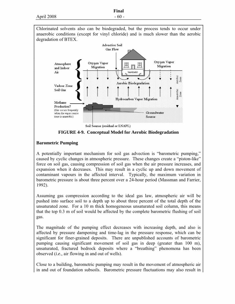
April 2008 - 60 -

Final

Chlorinated solvents also can be biodegraded, but the process tends to occur under anaerobic conditions (except for vinyl chloride) and is much slower than the aerobic degradation of BTEX.

FIGURE 4-9. Conceptual Model for Aerobic Biodegradation

Barometric Pumping

A potentially important mechanism for soil gas advection is “barometric pumping,” caused by cyclic changes in atmospheric pressure. These changes create a “piston-like” force on soil gas, causing compression of soil gas when the air pressure increases, and expansion when it decreases. This may result in a cyclic up and down movement of contaminant vapours in the affected interval. Typically, the maximum variation in barometric pressure is about three percent over a 24-hour period (Massman and Farrier, 1992).

Assuming gas compression according to the ideal gas law, atmospheric air will be pushed into surface soil to a depth up to about three percent of the total depth of the unsaturated zone. For a 10 m thick homogeneous unsaturated soil column, this means that the top 0.3 m of soil would be affected by the complete barometric flushing of soil gas.

The magnitude of the pumping effect decreases with increasing depth, and also is affected by pressure dampening and time-lag in the pressure response, which can be significant for finer-grained deposits. There are unpublished accounts of barometric pumping causing significant movement of soil gas in deep (greater than 100 m), unsaturated, fractured bedrock deposits where a “breathing” phenomena has been observed (i.e., air flowing in and out of wells).

Close to a building, barometric pumping may result in the movement of atmospheric air in and out of foundation subsoils. Barometric pressure fluctuations may also result in

April 2008 - 61 -

Final

episodic soil gas intrusion. If there is a low permeability surface seal adjacent to buildings, cross-foundation slab pressure gradients may be generated when the barometric pressure decreases. One study reported measured transient cross-slab differential pressures of up to 500 Pascals (Adomait and Fugler, 1997).

Stack and Wind Effect

The heating of a building, either by furnace, radiator, or other sources (i.e., sunlight on the roof) creates a “stack effect” as warm air rises in the building (Figure 4-10). This causes an outward air pressure in upper storeys and inward air pressure near the base of the building. Warm air that escapes is replaced by air infiltrating through doors and windows and soil gas migrating through the foundation. The magnitude of the depressurization at the base of the building is proportional to the height of the building, although tall buildings are designed with features to minimize cross-floor leakage of air and excessive depressurization.

Elevator shafts may represent both a preferential pathway for soil gas intrusion at the base of the building (a drain is often present in the elevator pit) and for upward movement of air within the building. The force of wind on the side of a building will cause a positive pressure on the windward side of the building and a negative pressure on the lee side thus potentially resulting in a depressurised building.

FIGURE 4-10. Stack and Wind Effect on Depressurisation

(NPL = neutral pressure line)

April 2008 - 62 -

Final

Foundation Construction

Conceptually, different foundation construction could lead to different processes for soil vapour intrusion. For example, higher soil gas advection rates would be expected for houses with basements, due to higher depressurization and larger subsurface foundation surface area for intrusion. For houses with crawlspace foundations, the degree to which the crawlspace is ventilated by outside air and the influence of cross-floor mixing and leakage between the crawlspace and main floor could affect soil vapour intrusion rates. In cold climate areas, crawlspaces are more likely to be well sealed to reduce the influx of cold air into the house. Buildings with earthen floors are especially prone to vapour intrusion since there is a large surface area for migration of soil vapour into the overlying structure; however, openings around utilities and a perimeter crack, often observed at the interface between the foundation wall and floor slab, also represent potentially significant entry routes for soil gas migration.

Although working hypotheses have been developed, the influence of foundation type on soil vapour intrusion is still poorly understood. However, there are empirical data indicating that soil vapour intrusion can be significant for several different types of building foundations including basements, crawlspaces and slab-on-grade construction. The importance of the foundation for vapour intrusion may depend on the distance from the contamination source to the building; for larger distances the foundation may have little effect on vapour intrusion rate; for smaller distances or where contamination is close to or in direct contact with the building (e.g., sumps, wet basements), the foundation properties will tend to be significant.

Condominiums or commercial buildings may have one or more levels of below-grade parking. Since ventilation rates are high for parking garages, there will tend to be greater dilution of vapours that may migrate into the garage than for other building types.

Temporal and Seasonal Considerations

Potential temporal factors influencing soil vapour intrusion are complex. Higher building depressurization and soil gas intrusion rates would be expected during the heating season. Winter frost or higher soil moisture in near surface soils may limit the surface flux of volatiles to the atmosphere. As a consequence, the migration of soil vapour toward drier soils below the building may be enhanced. In some cases, intensive snowmelt or rain and wetting fronts can induce advective movement of soil gas, which may, in turn, cause nonequilibrium mass transfer of the contaminants between the water and the gas phases (Cho et al., 1993).

Surface soils with high moisture content may also reduce migration of atmospheric oxygen into soil, which may reduce aerobic biodegradation of hydrocarbon vapours. An off-setting factor is that during summer, near surface ground temperatures may be higher leading to slightly higher volatilization rates, since the Henry’s Law Constant is temperature dependent. The amplitude in seasonal temperature variation decreases with increasing depth below ground surface, and at many sites, temperature effects will be insignificant.

April 2008 - 63 -

Final

The influence of seasonal factors on building ventilation, which acts to dilute vapours, is difficult to predict. While natural ventilation through open doors or windows may be reduced in winter, there may be increased air exchange through building depressurization and operation of a furnace. There can also be significant short-term variability unrelated to seasonal factors caused by diurnal temperature fluctuations, occupant use (e.g., opening windows and doors), wind, and barometric pressure variations. On balance, the above factors suggest that in Canada, soil vapour intrusion would tend to be greatest during winter months based on climatic conditions.

Buildings and Tanks as Soil Vapour Sources

While the usual paradigm for soil vapour transport is upward migration from a contamination source located at or near the water table, if there is a surface contamination source, vapours will migrate in all directions, including downwards. Indoor air that is affected by contamination sources within a building may affect subsurface vapour concentrations if the building is positively pressurized (McHugh et al., 2006). In this case, air will move downwards through the foundation. Once below the building, vapours could diffuse away from the building, thus creating a zone of impacted soil vapour. While it would be rare for buildings to have a significant effect on subsurface soil vapour concentrations, a dry cleaner is one possible example of where this could occur. Leaking underground storage tanks also represent potential soil vapour sources.

4.5 References

Abreu , L. 2005. A Transient Three Dimensional Numerical Model To Simulate Vapor Intrusion Into Buildings. A Dissertation Presented in Partial Fulfillment of the Requirements for the Degree Doctor of Philosophy, Arizona State University, May 2005.

Adomait, M. and D. Fugler. 1997. A Method to Evaluate Vapour Influx into Houses. Presented at AWMA 90th Meeting, June 8 to 13, Toronto, Ontario, Canada.

Agriculture and Agri-Food Canada, 2000. The health of our water - toward sustainable agriculture in Canada. Edited by Coote D.R. and L.J. Gregorich, Publication 2020/E.

Anderson, M. R., R. L. Johnson, and J. F. Pankow, 1992. Dissolution of dense chlorinated solvents into ground water: 1. Dissolution from a well-defined residual source. Ground Water 30(2), pp. 250-256.

Auer, L.H., Rosenberg, N.D., Birdsell, K.H., and Whitney, E.M., 1996. The effects of barometric pumping on contaminant transport. J. Contaminant Hydrology. 24:145-166.

April 2008 - 64 -

Final

Bradley, P.M., S.A. Carr, S.A., R.B. Baird and F.H. Chapelle, 2005. Biodegradation of N-nitrosodimethylamine in soil from a water reclamation facility. Bioremediation Journal, 9, (2) : 115-120.

Canadian Council of Ministers of the Environment, 2008. Canada-Wide Standards for Petroleum Hydrocarbon (PHC) in Soil. Endorsed by CCME Council of Ministers, Winnipeg.

Charbeneau, R.J. and D.E. Daniel, 1993. Contaminant Transport in Unsaturated Zone (Chapter 15). In Handbook of Hydrology. David Maidment. Editor in Chief. McGraw Hill, New York.

Choi, J.W. and J. A. Smith 2005. Geoenvironmental Factors Affecting Organic Vapor Advection and Diffusion Fluxes from the Unsaturated Zone to the Atmosphere under Natural Conditions. Environmental Engineering Science Volume 22, Number 1, 2005 © Mary Ann Liebert, Inc.

Chiou, C.T., L.J. Peters and V.H. Freed. 1979. A physical concept of soil-water equilibrium for non-ionic organic compounds. Science 206:831-832.

Cho, H.J., Jaffe, P.R., and Smith, J.A., 1993. Simulating the volatilization of solvents in unsaturated soils during laboratory and field infiltration experiments. Water Resources Research, 29 (10) :3329-3342.

Crowe, A.S., K.A. Schaefer, A. Kohut, S.G. Shikaze and C.J. Ptacek. 2003. Groundwater Quality. Canadian Council of Ministers of the Environment, Winnipeg, Manitoba, CCME Linking Water Science to Policy Workshop Series, Report No. 2, 52 p.

Domenico, P.A. and F.W. Schwartz, 1998. Physical and Chemical Hydrogeology. 2nd Edition. John Wiley and Sons, Inc.

Environment Canada, 2002. Assessment Report - N-Nitrosodimethylamine. Canada Gazette, Part 1 April 13. http://www.ec.gc.ca/substances/ese/eng/psap/final/NDMA.cfm

Falta, R.W., B. Bulsara, J.L. Henderson and R.A. Mayer, 2005. Leaded-Gasoline Additives Still Contaminate Groundwater. Environ. Sci. and Technol., 39 (18): 379A-384A

Fetter, C.W., 2004. Applied Hydrogeology. Prentice Hall.

Garbesi, K., R.G. Sextro, W.J. Fisk, M.P. Modera, and K.L. Revzan. 1993. Soil-Gas Entry into an Experimental Basement: Model Measurement Comparisons and Seasonal Effects. Environ. Sci. Technol. 27(3): 466-473.

April 2008 - 65 -

Final

Government of Canada (2003), Canadian Framework for Collaboration on Groundwater, at p. 1.

Gorgy, T.A., L. Li and J. Grace (2006) Fate and Transport of Polybrominated Biphenyl Ethers from Biosolids. ISSMGE 5th International Conference on Environmental Geotechnics, Cardiff, Wales.

Hassett, J.J. and W.L. Banwart. 1989. The sorption of nonpolar organics by soils and sediments. In: Reactions and movement of organic chemicals in soils. Sawney, B.L. and K. Brown, eds. SSSA Spec. Publ. 22. Soil Science Society of America Inc., Madison, WI.

Hassett, J.J., J.C. Means, W.L. Banwart and S.G. Wood. 1980. Sorption properties of sediments and energy-related pollutants. EPA-600/3-80-041. U.S. Environmental Protection Agency, Washington, DC.

Health Canada, 2007. Federal Contaminated Site Risk Assessment in Canada Part I: Guidance on Human Health Preliminary Quantitative Risk Assessment (PQRA).

Health Canada, Draft 2008. Federal Contaminated Site Risk Assessment in Canada, PQRA Part VIII: Guidance for Soil Vapour Intrusion at Contaminated Sites

Hers, I., Zapf-Gilje, R., Johnson, P.C. and Li, L. 2003. Evaluation of the Johnson and Ettinger Model for Prediction of Indoor Air Quality. Ground Water Monitoring and Remediation, 23(2): 119-133.

Hers, I., J. Atwater, L. Li and R. Zapf-Gilje. 2000. Evaluation of vadose zone biodegradation of BTX vapours. Journal of Contaminant Hydrology, 46: 233-264.

Hers, I., Evans, D, Zapf-Gilje, R. and Li, L. 2002. Comparison, Validation and Use of Models for Predicting Indoor Air Quality from Soil and Groundwater Contamination. Journal of Soil and Sediment Contamination, 11 (4): 491-527.

Johnson, P.C. 2005. Identification of application-specific critical inputs for the 1991 Johnson and Ettinger vapor intrusion algorithm. Groundwater Monitoring & Remediation, 25(1): 63-78.

Johnson, P.C., W. Kemblowski, and R.L. Johnson. 1998. Assessing the Significance of Subsurface Contaminant Vapour Migration to Enclosed Spaces – site specific alternatives to generic estimates. API Publication.

Lowell, P.S. and Eklund, B. 2004. VOC Emission Fluxes as a Function of Lateral Distance from the Source. Environmental Progress. 23 (1): 52-58

April 2008 - 66 -

Final

Massman, J. and D.F.Farrier. 1992. Effects of Atmospheric Pressures on Gas Transport in the Vadose Zone. Water Resources Research 28: 777-791.

McHugh, T., P. C. De Blanc and R.J. Pokluda, 2006. Indoor Air as a Source of VOC Contamination in Shallow Soils Below Buildings. Journal of Soil & Sediment Contamination, 15: 103-122.

Mendoza, C. A. 1995. Conceptual Models and Effective Transport Parameters for Long-term Vapour Transport in Heterogeneous Unsaturated Media. Presented at: Solutions ’95 IAH International Congress XXVI, June 5-9, 1995, Edmonton, Alberta.

Millington, R.J. and J.M. Quirk. 1961. Permeability of porous solids. Transactions of the Farady Society, 57: 1200-1207.

National Research Council of Canada, 1988. Glossary of Permafrost and Related Ground-ice Terms. Technical Memorandum No. 142. Associate Committee on Geotechnical Research. Permafrost Subcommittee, Ottawa.

National Research Council (US), 1996. Rock Fractures and Fluid Flow: Contemporary Understanding and Applications. Committee of Fracture Characterization and Fluid Flow, U.S. National Committee for Rock Mechanics. National Academy Press, Washington, D.C.

Ostendorf, D.W. and D.H. Campbell. 1991. Biodegradation of hydrocarbon vapours in the unsaturated zone. Water Resources Research. 27 (4):453-462.

Park, H. S. and San Juan, C., 2000. A Method for Assessing Leaching Potential for Petroleum Hydrocarbons Release Sites, Soil and Sediment Contamination, 9(6):611-632.

Ririe, T., R. Sweeney, S. Daughery, and P. Peuron. (1998) A Vapour Transport Model That is Consistent with Field and Laboratory Data. In Proceedings: Petroleum Hydrocarbons and Organic Chemicals in Ground Water: Prevention, Detection, and Remediation Conference. Ground Water Association Publishing, Houston, TX: 299-308

Robinson, R. A., and R.H. Stokes, 1959. Electrolyte solutions. Butterworths, London.

Roggemans, S., C.L. Bruce, and P.C. Johnson. 2002. Vadose Zone Natural Attenuation of Hydrocarbon Vapors: An Empirical Assessment of Soil Gas Vertical Profile Data. American Petroleum Institute Technical Report.

Rivett, M. O., 1995. Soil-gas signatures from volatile chlorinated solvents: Borden field experiments. Ground Water 33(1): 84-98.

April 2008 - 67 -

Final

Schwartz, W., and H. Zhang. 2002. Fundamentals of Ground Water. 1st ed. John Wiley & Sons. 592pp.

Schwarzenbach, R.P, P.M. Gschwend and D.M. Imboden, 2003. Environmental Organic Chemistry, John Wiley and Sons, Inc.

Science Advisory Board for Contaminated Sites (SABCS) (of British Columbia), 2006b. Approaches and Methods for Evaluation of Unsaturated Zone Contaminant Transport processes and Effects on Groundwater. Report prepared by Golder Associates Ltd. (Hers, I. and D. Fredlund), June.

Science Advisory Board for Contaminated Sites (SABCS) (of British Columbia), 2006a. Approaches and Methods for Evaluation of Light Non Aqueous Phase Liquid Mobility. Report prepared by Golder Associates Ltd. (Hers, I; G. Patrick and M. Mailloux), February.

Silliman, S.E., B. Berkowitz, J. Simunek and M.Th. van Genuchten (2002), Fluid flow and chemical migration within the capillary fringe, Ground Water 40 (1), pp. 76–84.

Snow, D.T., 1968. Rock fracture spacings, openings and porosities. J. Soil Mech. Found. Div. Proc. Am. Soc. Civil Eng. 94: 73–91.

United States Environmental Protection Agency (USEPA). 2002. Draft Guidance for Evaluating the Vapor Intrusion to Indoor Air Pathway from Groundwater and Soils (Subsurface Vapour Intrusion Guidance). Office of Solid Waste and Emergency Response.

United States Environmental Protection Agency (USEPA). 1996. Soil Screening Guidance: Technical Background Document, EPA/540/R95/128. available at http://www.epa.gov/superfund/resources/soil/toc.htm

Wiedemeier, T.H., H.S. Rafai, J.T. Wilson and C.J. Newell, 1999. Natural Attenuation of Fuels and Chlorinated Solvents in the Subsurface, John Wiley and Sons, Inc., 617 pg.

Zheng, C. and G.D. Bennett, 1995. Applied Contaminant Transport Modeling: Theory and Practice. Van Nostrand Reinhold.

April 2008 - 68 -

Final

5.0 SOIL CHARACTERIZATION GUIDANCE

5.1 Context, Purpose and Scope

Soil is the main medium where contamination resides (source) and from where contaminants partition into groundwater and soil vapour. Understanding the presence, extent and characteristics of contamination in soil is therefore critical for understanding the ultimate fate and potential impact of the contamination on human and ecological receptors. For example, the measurement of chemical concentrations in soil may be required to evaluate potential human exposure through direct exposure pathways such as ingestion and dermal contact. The characterization of soil may also be required to evaluate the potential effect of contamination in soil on other media such as groundwater, soil vapour, indoor air and ambient air.

The primary purpose of this soil investigation guidance is to describe the approach and methods for acquiring representative data (Exhibit 5-1). Obtaining representative data is closely linked to the sampling design, which involves consideration of the scale at which samples are analyzed. The sources of uncertainty in data should be understood, and effectively communicated to the risk assessor. Uncertainties may include those due to the variability in the contaminant distribution, those introduced through the sampling design, and methods used for sampling and analysis. As subsequently described in this chapter, uncertainty is reduced through the development of a conceptual site model that is updated as new information is obtained, an appropriate soil sampling strategy and design, and through statistical techniques to assist in sampling design and data interpretation.

The characterization of soil at contaminated sites should follow the characterization process described in Chapter 2, as outlined in the above text box. The guidance does not address laboratory analytical protocols since for most chemical constituents, standardized methods are employed and information on these methods is readily available (see Section 4.1 of the guidance). While the focus of this chapter is intrusive soil sampling, indirect methods such as geophysical techniques can be used to help to identify potential contamination zones and provide stratigraphic information. Guidance on confirmation of remediation sampling is provided in Appendix 5-1 to this chapter.

Soil Characterization

This chapter describes the planning, process and methods for soil characterization. The key elements and their corresponding sections in the chapter are:

Conceptual site model development (5.2),

Sampling design considerations and statistical methods (5.3),

Recommendations for selection of sampling design (5.4),

Soil sampling methods, soil description and field analytical methods (5.5 to 5.7),

Data validation and interpretation (5.8), and

Tools for soil sampling design (5.9).

Related tools are the Soil Sampling Checklists in Volume 2 and Suggested Operating Procedure for Soil Sampling (SOP-2) in Volume 3.

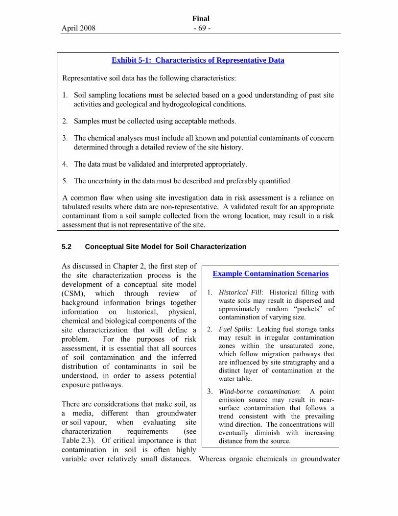
April 2008 - 69 -

Final

5.2 Conceptual Site Model for Soil Characterization

As discussed in Chapter 2, the first step of the site characterization process is the development of a conceptual site model (CSM), which through review of background information brings together information on historical, physical, chemical and biological components of the site characterization that will define a problem. For the purposes of risk assessment, it is essential that all sources of soil contamination and the inferred distribution of contaminants in soil be understood, in order to assess potential exposure pathways.

There are considerations that make soil, as a media, different than groundwater or soil vapour, when evaluating site characterization requirements (see Table 2.3). Of critical importance is that contamination in soil is often highly variable over relatively small distances. Whereas organic chemicals in groundwater

Example Contamination Scenarios

1. Historical Fill: Historical filling with waste soils may result in dispersed and approximately random “pockets” of contamination of varying size.

2. Fuel Spills: Leaking fuel storage tanks may result in irregular contamination zones within the unsaturated zone, which follow migration pathways that are influenced by site stratigraphy and a distinct layer of contamination at the water table.

3. Wind-borne contamination: A point emission source may result in near- surface contamination that follows a trend consistent with the prevailing wind direction. The concentrations will eventually diminish with increasing distance from the source.

Exhibit 5-1: Characteristics of Representative Data

Representative soil data has the following characteristics:

1. Soil sampling locations must be selected based on a good understanding of past site activities and geological and hydrogeological conditions.

2. Samples must be collected using acceptable methods.

3. The chemical analyses must include all known and potential contaminants of concern determined through a detailed review of the site history.

4. The data must be validated and interpreted appropriately.

5. The uncertainty in the data must be described and preferably quantified.

A common flaw when using site investigation data in risk assessment is a reliance on tabulated results where data are non-representative. A validated result for an appropriate contaminant from a soil sample collected from the wrong location, may result in a risk assessment that is not representative of the site.

April 2008 - 70 -

Final

tend to form plumes in a relatively predictable manner, soil contamination may be discontinuous and dispersed depending on the contamination source. Temporal changes in soil concentrations tend to be slow and generally inconsequential; therefore, temporal considerations tend not to be important for soil contamination.

Insight on the distribution of contaminants in soil can be gained through an understanding of the contamination source, contaminant type and site geology. Several examples illustrating the variability in contamination scenarios are described in the Example Contamination Sources text box. The contaminant distribution in soil will also depend on the site geology and heterogeneity. For example, soil contamination in fractured rock will be highly variable, whereas, soil contamination in deltaic sand deposits will tend to be less variable.

The elements or components of the CSM should follow those listed in Table 2.1. Of particular importance for characterization of soil is information on filling at the site and soil layering. As intrusive investigations are completed at a site, the CSM should be updated, and data gaps and information requirements should be re-defined. Several phases of investigation may be necessary before the investigation objectives are finally satisfied, although as described in Chapter 2, an expedited site investigation process may be followed to reduce the number of phases required.

5.3 Soil Sampling Design Considerations

As described in the sections below, the design of a soil sampling program for investigation of contaminated sites involves consideration of the objectives for soil sampling, the type of sampling design used to investigate the site, as supported by statistical methods where appropriate, and sample support or type (i.e., discrete versus composite). After these considerations are described, recommendations for selecting a sampling design, sample spacing and frequency of sample collection are provided.

5.3.1 Sampling Design Objectives

The sampling design is a fundamental part of the site characterization process. The sampling design describes the number of samples, and where and when samples should be collected. The goal of the sampling design is to provide representative data that are defensible for their intended use and decisions to be made. Representativeness may be considered as the degree to which data accurately and precisely represents the relevant characteristics of the target population. As a general rule, the representativeness of a sampling program increases and the uncertainty decreases as the number of samples analyzed increases.

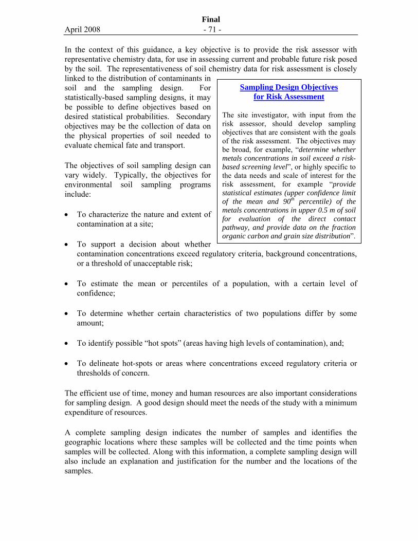
April 2008 - 71 -

Final

In the context of this guidance, a key objective is to provide the risk assessor with representative chemistry data, for use in assessing current and probable future risk posed by the soil. The representativeness of soil chemistry data for risk assessment is closely linked to the distribution of contaminants in soil and the sampling design. For statistically-based sampling designs, it may be possible to define objectives based on desired statistical probabilities. Secondary objectives may be the collection of data on the physical properties of soil needed to evaluate chemical fate and transport.

The objectives of soil sampling design can vary widely. Typically, the objectives for environmental soil sampling programs include:

• To characterize the nature and extent of contamination at a site;

• To support a decision about whether contamination concentrations exceed regulatory criteria, background concentrations, or a threshold of unacceptable risk;

• To estimate the mean or percentiles of a population, with a certain level of confidence;

• To determine whether certain characteristics of two populations differ by some amount;

• To identify possible “hot spots” (areas having high levels of contamination), and;

• To delineate hot-spots or areas where concentrations exceed regulatory criteria or thresholds of concern.

The efficient use of time, money and human resources are also important considerations for sampling design. A good design should meet the needs of the study with a minimum expenditure of resources.

A complete sampling design indicates the number of samples and identifies the geographic locations where these samples will be collected and the time points when samples will be collected. Along with this information, a complete sampling design will also include an explanation and justification for the number and the locations of the samples.

Sampling Design Objectives for Risk Assessment

The site investigator, with input from the risk assessor, should develop sampling objectives that are consistent with the goals of the risk assessment. The objectives may be broad, for example, “determine whether metals concentrations in soil exceed a risk-based screening level”, or highly specific to the data needs and scale of interest for the risk assessment, for example “provide statistical estimates (upper confidence limit of the mean and 90th percentile) of the metals concentrations in upper 0.5 m of soil for evaluation of the direct contact pathway, and provide data on the fraction organic carbon and grain size distribution”.

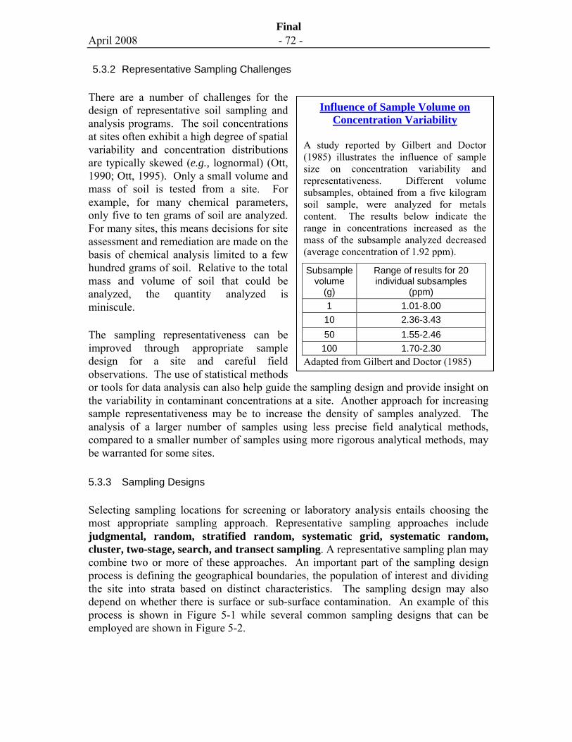
April 2008 - 72 -

Final

5.3.2 Representative Sampling Challenges

There are a number of challenges for the design of representative soil sampling and analysis programs. The soil concentrations at sites often exhibit a high degree of spatial variability and concentration distributions are typically skewed (e.g., lognormal) (Ott, 1990; Ott, 1995). Only a small volume and mass of soil is tested from a site. For example, for many chemical parameters, only five to ten grams of soil are analyzed. For many sites, this means decisions for site assessment and remediation are made on the basis of chemical analysis limited to a few hundred grams of soil. Relative to the total mass and volume of soil that could be analyzed, the quantity analyzed is miniscule.

The sampling representativeness can be improved through appropriate sample design for a site and careful field observations. The use of statistical methods or tools for data analysis can also help guide the sampling design and provide insight on the variability in contaminant concentrations at a site. Another approach for increasing sample representativeness may be to increase the density of samples analyzed. The analysis of a larger number of samples using less precise field analytical methods, compared to a smaller number of samples using more rigorous analytical methods, may be warranted for some sites.

5.3.3 Sampling Designs

Selecting sampling locations for screening or laboratory analysis entails choosing the most appropriate sampling approach. Representative sampling approaches include judgmental, random, stratified random, systematic grid, systematic random, cluster, two-stage, search, and transect sampling. A representative sampling plan may combine two or more of these approaches. An important part of the sampling design process is defining the geographical boundaries, the population of interest and dividing the site into strata based on distinct characteristics. The sampling design may also depend on whether there is surface or sub-surface contamination. An example of this process is shown in Figure 5-1 while several common sampling designs that can be employed are shown in Figure 5-2.

Influence of Sample Volume on Concentration Variability

A study reported by Gilbert and Doctor (1985) illustrates the influence of sample size on concentration variability and representativeness. Different volume subsamples, obtained from a five kilogram soil sample, were analyzed for metals content. The results below indicate the range in concentrations increased as the mass of the subsample analyzed decreased (average concentration of 1.92 ppm).

Subsample volume

(g)

Range of results for 20 individual subsamples

(ppm) 1 1.01-8.00 10 2.36-3.43 50 1.55-2.46

100 1.70-2.30 Adapted from Gilbert and Doctor (1985)

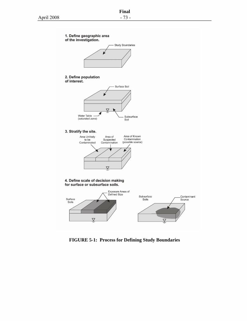
April 2008 - 73 -

Final

FIGURE 5-1: Process for Defining Study Boundaries

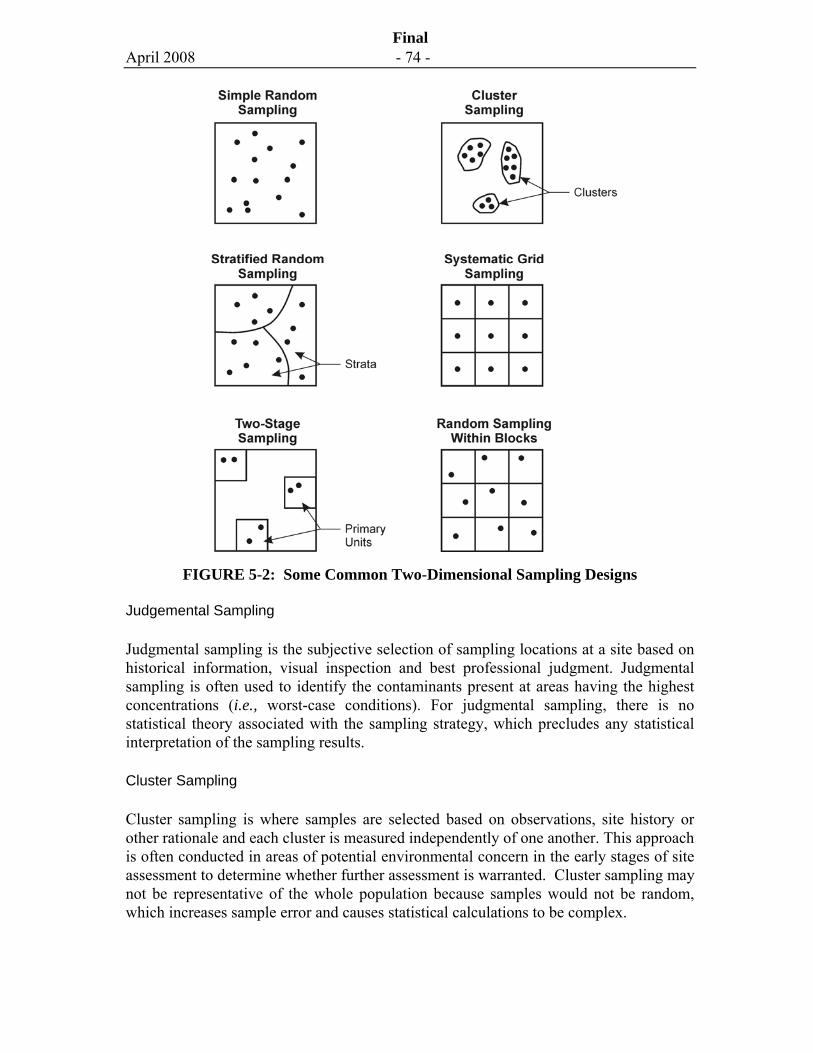
April 2008 - 74 -

Final

FIGURE 5-2: Some Common Two-Dimensional Sampling Designs

Judgemental Sampling

Judgmental sampling is the subjective selection of sampling locations at a site based on historical information, visual inspection and best professional judgment. Judgmental sampling is often used to identify the contaminants present at areas having the highest concentrations (i.e., worst-case conditions). For judgmental sampling, there is no statistical theory associated with the sampling strategy, which precludes any statistical interpretation of the sampling results.

Cluster Sampling

Cluster sampling is where samples are selected based on observations, site history or other rationale and each cluster is measured independently of one another. This approach is often conducted in areas of potential environmental concern in the early stages of site assessment to determine whether further assessment is warranted. Cluster sampling may not be representative of the whole population because samples would not be random, which increases sample error and causes statistical calculations to be complex.

April 2008 - 75 -

Final

Random Sampling

Random sampling is where the sampling units are selected using random numbers. There is equal probability of selection of all possible units within defined boundaries of the area of concern. Random sampling has two primary limitations: (i) because all sampling points have an equal chance of being selected, sampling locations are not evenly dispersed across the site and therefore sample location coverage may be poor, unless a very large number of samples are taken, and (ii) random sampling ignores prior information or professional knowledge in the sampling process. Since random sampling is relatively inefficient, it is rarely used for characterising soil contamination.

Two-Stage Sampling

Two-stage sampling involves taking samples (primary units) using the simple random sampling technique and then taking an aliquot of those samples (Gilbert, 1987). Two-stage sampling allows for a lower error than cluster sampling yet higher error than simple random sampling.

Stratified Sampling

Stratified sampling relies on historical information, screening and prior analytical results to divide the sampling area into smaller areas called strata. Each strata is more homogeneous than the site is as a whole. Strata can be defined based on various factors, including: historical site use and APECs, soil type, depth, contaminant concentration levels and knowledge on expected contaminant migration patterns for different media (e.g., groundwater, soil vapour, wind).

Systematic Grid Sampling

Systematic grid sampling involves subdividing the area of concern by using a square, rectangular or triangular grid and collecting samples from the nodes (i.e., intersections of the grid lines). The origin and orientation of the grid can be based on random selection. Systematic grid sampling is often used to delineate the extent of contamination and may be used to define contaminant concentration gradients. This design is also a practical method for designating sample locations and provides for uniform coverage of a site.

A potential shortcoming of grid sampling is the possibility of bias when there are cyclical patterns to contamination where the grid spacing is a multiple of the period to the concentration cycles. While this scenario is highly unlikely, if this is a potential concern, a different grid spacing for a portion of the site may be superimposed over the larger grid to assess this hypothesis.

April 2008 - 76 -

Final

Transect Sampling

Transect sampling is a special case of systematic grid sampling where certain specific spatial characteristics of the contamination are targeted. Contamination examples where transect sampling may be used are airborne deposits downwind from an emissions source (e.g., smokestack), contamination derived from vehicles along a roadway, and sediment along the base of a ditch. Since the concentration trends for each of the above scenarios will vary in a predictable manner, transects with appropriately spaced sampling locations can be used to effectively characterize linear trends.

5.3.4 Statistical Methods

While statistical tools are rarely rigorously used to design sampling programs, they can provide useful insight on the uncertainty in site characterization design and guidance on the number of samples to analyze. Three different statistical methods or tools that can be used for sampling design purposes are described below. Statistical methods for interpretation of data are described in Section 5.8.

Search Sampling

Search sampling utilizes a systematic grid sampling approach to search for areas where contaminants exceed applicable criteria. The number of samples and the grid spacing are determined on the basis of the acceptable level of error (i.e., the chance of missing a hot spot). Search sampling requires that assumptions be made about the size, shape, and depth of the hot spots. The smaller and/or narrower the hot spots are, the smaller the grid spacing must be in order to locate them. Also, the smaller the acceptable error of missing hot spots is, the smaller the grid spacing must be. This, in effect, means collecting more samples. Once a grid spacing has been selected, the probability of locating an elliptically-shaped hot spot can be estimated from Figure 5-3. Conversely, if the acceptable probability of missing a hot spot is specified, then the size of the hot spot which can be located at that probability level can be determined.

Search Sampling Grid Spacing Example

A historical review suggests the presence of buried waste on a site but the location is unknown. The waste area is assumed to be approximately circular in shape (S = 1) with a radius of 5 m (L = 5 m). The desired probability of not finding this hot-spot is 0.05. From Fig. 5-3, L/G is equal to 0.58. Therefore, the desired grid spacing is 8.6 m.

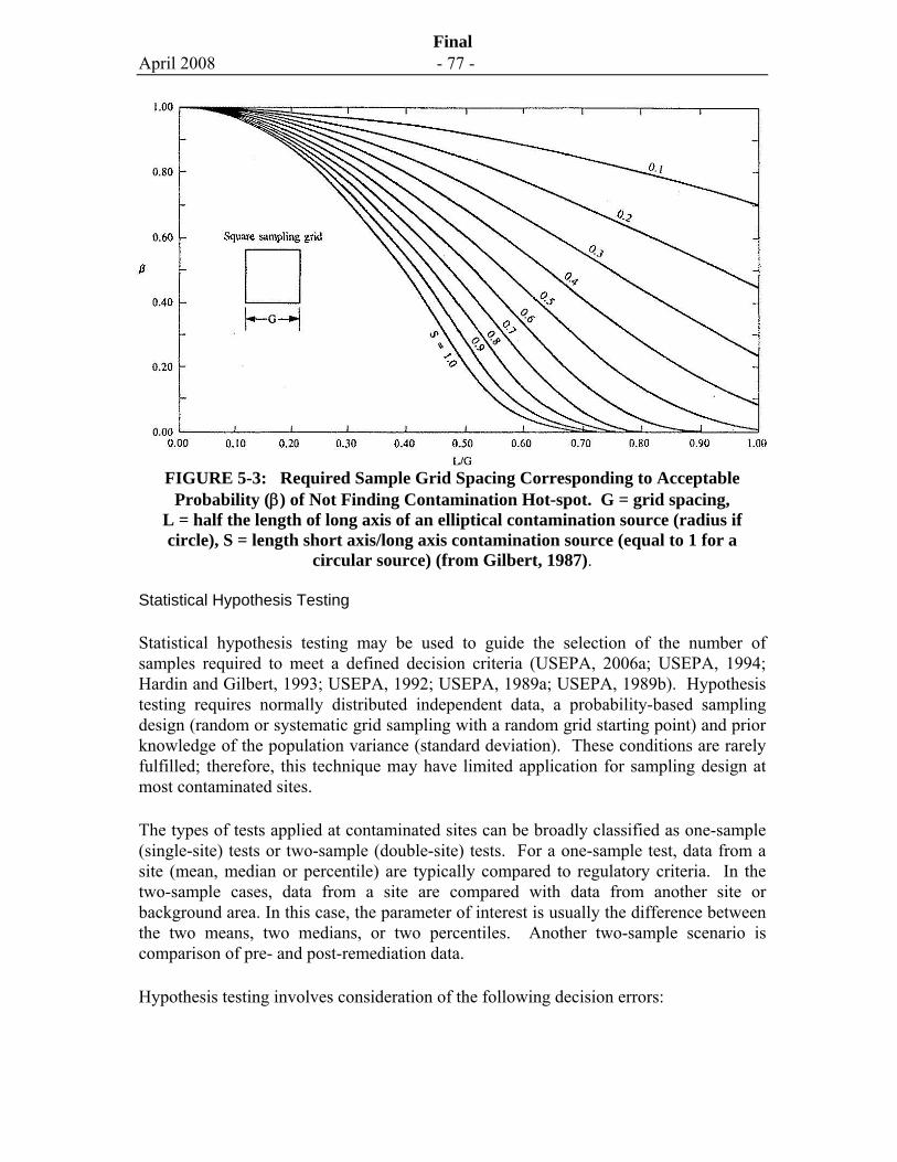
April 2008 - 77 -

Final

FIGURE 5-3: Required Sample Grid Spacing Corresponding to Acceptable Probability (β) of Not Finding Contamination Hot-spot. G = grid spacing,

L = half the length of long axis of an elliptical contamination source (radius if circle), S = length short axis/long axis contamination source (equal to 1 for a

circular source) (from Gilbert, 1987).

Statistical Hypothesis Testing

Statistical hypothesis testing may be used to guide the selection of the number of samples required to meet a defined decision criteria (USEPA, 2006a; USEPA, 1994; Hardin and Gilbert, 1993; USEPA, 1992; USEPA, 1989a; USEPA, 1989b). Hypothesis testing requires normally distributed independent data, a probability-based sampling design (random or systematic grid sampling with a random grid starting point) and prior knowledge of the population variance (standard deviation). These conditions are rarely fulfilled; therefore, this technique may have limited application for sampling design at most contaminated sites.

The types of tests applied at contaminated sites can be broadly classified as one-sample (single-site) tests or two-sample (double-site) tests. For a one-sample test, data from a site (mean, median or percentile) are typically compared to regulatory criteria. In the two-sample cases, data from a site are compared with data from another site or background area. In this case, the parameter of interest is usually the difference between the two means, two medians, or two percentiles. Another two-sample scenario is comparison of pre- and post-remediation data.

Hypothesis testing involves consideration of the following decision errors:

April 2008 - 78 -

Final

• The null hypothesis (baseline condition) is rejected when it is actually true, which is a false rejection (Type I) decision error. The probability of this error occurring is called alpha (α) and is called the hypothesis test’s level of significance.

• The null hypothesis is not rejected when it is actually false, which is a false acceptance (Type II) decision error. The probability that this error will occur is called beta (β). The probability of rejecting the null hypothesis when it is actually false (1-β) is referred to as the statistical power.

An example is where a mean concentration of a contaminant in soil should not exceed a regulatory criterion. The null hypothesis may be formulated as the true mean concentration is equal to or exceeds the criteria, while the alternative hypothesis is that the true mean is less than the criteria.3 If one concludes that the mean concentration is less than the criteria when the true mean exceeds the criteria, then a Type I error has been committed. If one concludes that the mean concentration exceeds the criteria when the true mean is less than the criteria, then a Type II error has been committed. In this context, a Type I error may result in health risks not being adequately addressed, whereas a Type II error may result in needless remediation and resource expenditure.

Sample size formulas for different hypothesis tests are provided in USEPA (2002). The sample size formula for an one-sided t-test of the mean used to determine the minimum number of samples, n, required to achieve a specified confidence level at a defined minimum detectable relative difference (i.e., precision) may be estimated by the following equation:

n ≥ [ (Z1-α + Z1-β) CV/D ]2 + [ 0.5Z1-α ] 2 [Eq 5.1]

3 Depending on the project objectives, the formulation of hypotheses could be reversed, i.e., the null hypothesis is the true mean concentration is less than or equal to the criteria, and the alternative hypothesis is the true mean concentration exceeds the criteria.

Example of Statistically-Based Estimate Minimum Sample Number

Lead contamination is associated with refinery sludge deposited at a site. The contamination is believed to be approximately randomly distributed within the fill. The desired confidence level (1-α) and power (1-β) are 95 and 80 percent, respectively. The CV is estimated to range from 0.5 to 1, considered a reasonable range for a well-characterized site with reasonably uniform contamination. The applicable regulatory criterion for lead is 500 mg/kg. D is assumed to be 0.2, or a minimum detectable difference of 100 mg/kg (i.e., mean value between 400 and 500 mg/kg). The minimum number of samples (Eq. 5.1) to fulfill the specified confidence level and power is between 40 and 155, for a CV between 0.5 and 1. This example illustrates the large number of samples that may be required to meet statistically-based criteria.

April 2008 - 79 -

Final

Where Z1-α and Z1-β are the standard normals, CV is the coefficient of variation (dimensionless ratio) and D is the minimum detectable relative difference (dimensionless ratio). In practical terms, the minimum detectable relative difference is the “grey zone” or range where it is not possible to distinguish the true mean from the regulatory criterion or action level. A reasonable value for D may be 20 percent of the action level (0.2). The CV can be estimated from previous studies at the site of interest or other similar sites. A rough approximation is provided by the following equation (USEPA, 2002):

CV = [ ( Maximum – Minimum) / 6 ] / Average [Eq 5.2]

Where the maximum, minimum and average are expected concentrations for the population being sampled.

The same statistical principles that underlie hypothesis tests can be applied to the interpretation of confidence limits of the mean. For example, suppose a one-sided 95% upper confidence limit of the mean exceeds the regulatory criteria. One would conclude that the null hypothesis could not be rejected, and would instead accept that the true mean could exceed the regulatory criteria at the 0.05 significance level.

Geostatistical Methods

The statistical hypothesis testing described above assumes independent data that are not spatially correlated. When there is a spatial dependence, concentrations of nearby samples will change less dramatically than those for samples spaced farther apart. If there is a significant spatial dependence relative to the sample grid spacing employed, sampling following a systematic grid design will produce biased estimates of the mean if they are not adjusted for the degree of spatial continuity (USEPA, 2002).

For many contaminated sites, geostatistical methods are of limited application since there is often no or only limited spatial dependence in concentrations for practically achievable sampling grids. One example where geostatistical methods have been successfully employed is evaluation of wind-borne metals (zinc) contamination of surface soil from a point emission source (e.g., Palmerton Superfund site, USEPA 1989b; Hirotaka and Goovaerts, 2001).

When there is a predictable spatial dependence over the scale of interest, geostatistical methods can be used to quantify spatial dependences and to contour concentration data. In simple terms, geostatistical analysis involves a two-step process. First, the spatial dependence in data is quantified through the use of a variogram or semi-variogram. The variogram is a plot of the variance of paired sample measurements as a function of the distance between samples. When there is little distance between points, the variability between points will be small. As the distance between points increases, the difference or variability between points increases. A variogram model is fit to the empirical data based on the observed relationship. From the empirical data and variogram model, the distance over which there is a spatial correlation in the data is determined. The second

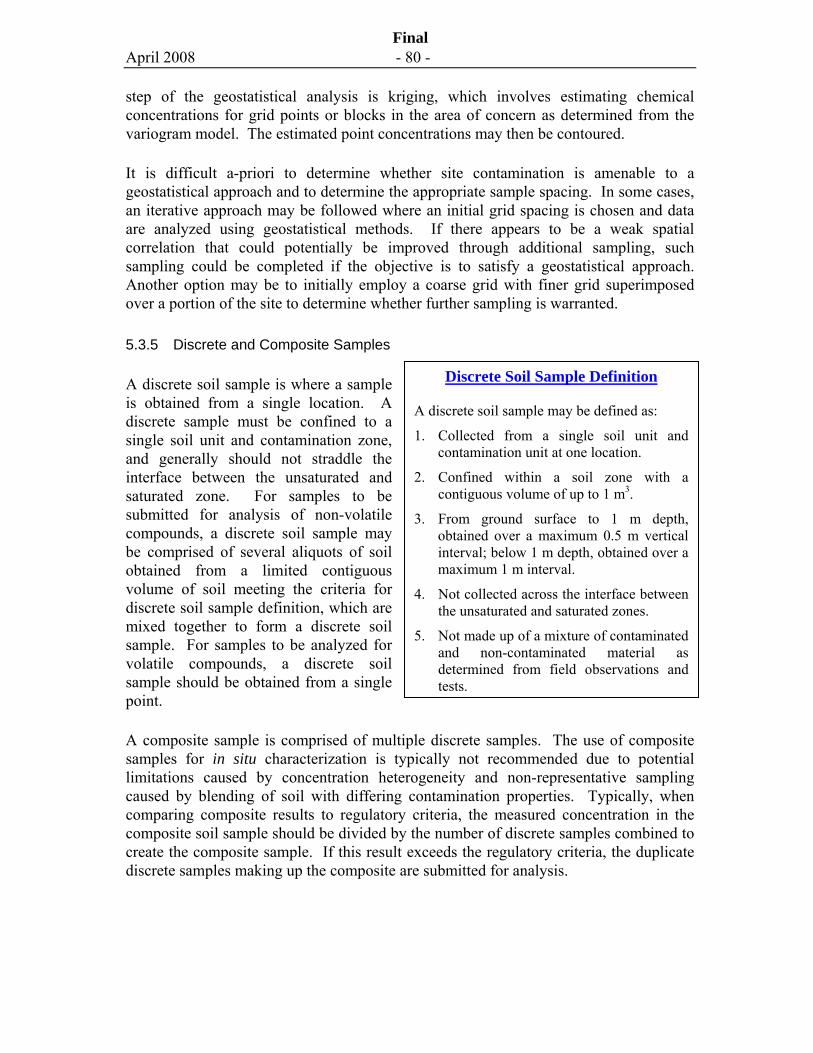
April 2008 - 80 -

Final

step of the geostatistical analysis is kriging, which involves estimating chemical concentrations for grid points or blocks in the area of concern as determined from the variogram model. The estimated point concentrations may then be contoured.

It is difficult a-priori to determine whether site contamination is amenable to a geostatistical approach and to determine the appropriate sample spacing. In some cases, an iterative approach may be followed where an initial grid spacing is chosen and data are analyzed using geostatistical methods. If there appears to be a weak spatial correlation that could potentially be improved through additional sampling, such sampling could be completed if the objective is to satisfy a geostatistical approach. Another option may be to initially employ a coarse grid with finer grid superimposed over a portion of the site to determine whether further sampling is warranted.

5.3.5 Discrete and Composite Samples

A discrete soil sample is where a sample is obtained from a single location. A discrete sample must be confined to a single soil unit and contamination zone, and generally should not straddle the interface between the unsaturated and saturated zone. For samples to be submitted for analysis of non-volatile compounds, a discrete soil sample may be comprised of several aliquots of soil obtained from a limited contiguous volume of soil meeting the criteria for discrete soil sample definition, which are mixed together to form a discrete soil sample. For samples to be analyzed for volatile compounds, a discrete soil sample should be obtained from a single point.

A composite sample is comprised of multiple discrete samples. The use of composite samples for in situ characterization is typically not recommended due to potential limitations caused by concentration heterogeneity and non-representative sampling caused by blending of soil with differing contamination properties. Typically, when comparing composite results to regulatory criteria, the measured concentration in the composite soil sample should be divided by the number of discrete samples combined to create the composite sample. If this result exceeds the regulatory criteria, the duplicate discrete samples making up the composite are submitted for analysis.

Discrete Soil Sample Definition A discrete soil sample may be defined as:

1. Collected from a single soil unit and contamination unit at one location.

2. Confined within a soil zone with a contiguous volume of up to 1 m3.

3. From ground surface to 1 m depth, obtained over a maximum 0.5 m vertical interval; below 1 m depth, obtained over a maximum 1 m interval.

4. Not collected across the interface between the unsaturated and saturated zones.

5. Not made up of a mixture of contaminated and non-contaminated material as determined from field observations and tests.

April 2008 - 81 -

Final

5.4 Selection of Sampling Design for Soil Investigation

The selection of a sampling design for site characterization involves integrating the available site information and knowledge on the contamination source, the conceptual site model including the expected contaminant distribution, sampling design objectives and statistical evaluations to identify a sampling design that best satisfies the goals of the site investigation and risk assessment. An incorrect sampling design will produce non-representative data and hence can not be used for risk assessment. The considerations for selecting a sampling design are described below.

5.4.1 Preliminary Investigation Sampling

The preliminary investigation sampling program should target the APECs and COPCs identified as part of the initial review phase of the project (i.e., Phase I Environmental Site Assessment).

Typically, the three most prevalent sampling designs for early stages of an investigation of potential soil contamination are judgmental sampling, systematic grid sampling and transect sampling. Often a combination of the above approaches is used.

Judgmental sampling is appropriate for sites where there is historical information, visual indicators or other data that can be used to identify sample locations. There may also be localized contamination sources such as spills, tanks or other facilities. A potential disadvantage of judgmental sampling is that statistical inferences cannot be made since it is not a probability-based sampling method. A common example is the investigation of an underground storage tank, which would typically involve step-out sampling of soil and groundwater around the tank in the inferred downgradient groundwater direction.

Systematic grid sampling is commonly used over larger areas where contamination is dispersed and where there is a need to provide for sufficient sample coverage. Guidelines for sample spacing are provided in Figure 5-3 and Exhibit 5.2. Contamination scenarios where systematic sampling may be appropriate include fill deposits, surface contamination from airborne deposits or other surface deposition, and lagoons. When the initial starting point to the grid is randomly selected, systematic grid sampling is a probability-based method that may be used to derive statistical inferences. Grid sampling may also be used to delineate concentration gradients and trends.

Transect sampling, a special case of systematic sampling, is a valid approach where contamination is inferred to exhibit strong trends along a linear profile; such as air borne contamination that would preferentially occur along prevalent wind directions in relation to the release point.

April 2008 - 82 -

Final

At the completion of the preliminary investigation phase, the data should be validated and interpreted and where appropriate, statistical parameters should be calculated. For investigations where the sampling design supports a statistical analysis of data (e.g., random or systematic grid sampling) and where the data analysis indicates a single data population, a statistical approach may be adopted to calculate statistical parameters such as the upper confidence limit of the mean and 90th percentile for comparison to regulatory criteria. Where these statistical parameters exceed the regulatory criteria or the maximum concentration exceeds the criteria by a tolerable limit (e.g., 2X), delineation sampling will generally be warranted. These statistical methods are further described in Section 5.8.

5.4.2 Detailed Investigation Sampling

The detailed investigation sampling design will depend on the current CSM, including results of the preliminary sampling, statistical analysis (where relevant), site specific geology, contaminants of concerns or potential concern, location of potential contaminant source, release and transport mechanism. During the detailed stages of an investigation, contamination delineation (in situ) sampling is often employed to define the limits of contamination previously identified at a site. Such sampling should consider both the vertical and lateral distribution of contaminants. The lateral sampling design may depend on the size of the contamination area. For smaller hot-spots, several step-out samples evenly spaced in a radial pattern (i.e., spokes of a wheel) are typical used for delineation purposes. Sampling may also be guided by real-time measurement technologies, as appropriate.

If the data analysis indicates a dispersed contamination scenario that is part of a single population, further systematic grid sampling may be warranted on a closer spaced grid to improve the level of confidence in the data. The statistical analysis described in Section 5.8 should be performed to determine whether this approach is valid.

For comparison purposes, a reference background sample should also be collected away from the source of contamination.

Guidelines on sample spacing for both approaches described above are provided in Exhibit 5-2. Useful guidance on soil sampling design and statistical methods (consisting of twelve different statistical procedures) is provided in BC Ministry of Environment Technical Guidance for Contaminated Sites 12: Statistics for Contaminated Sites (BC MOE 2005a, http://www.env.gov.bc.ca/epd/remediation/guidance/technical/).

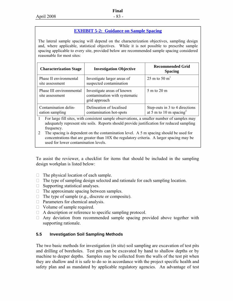
April 2008 - 83 -

Final

To assist the reviewer, a checklist for items that should be included in the sampling design workplan is listed below:

The physical location of each sample. The type of sampling design selected and rationale for each sampling location. Supporting statistical analyses. The approximate spacing between samples. The type of sample (e.g., discrete or composite). Parameters for chemical analysis. Volume of sample required. A description or reference to specific sampling protocol. Any deviation from recommended sample spacing provided above together with

supporting rationale. 5.5 Investigation Soil Sampling Methods

The two basic methods for investigation (in situ) soil sampling are excavation of test pits and drilling of boreholes. Test pits can be excavated by hand to shallow depths or by machine to deeper depths. Samples may be collected from the walls of the test pit when they are shallow and it is safe to do so in accordance with the project specific health and safety plan and as mandated by applicable regulatory agencies. An advantage of test

EXHIBIT 5-2: Guidance on Sample Spacing

The lateral sample spacing will depend on the characterization objectives, sampling design and, where applicable, statistical objectives. While it is not possible to prescribe sample spacing applicable to every site, provided below are recommended sample spacing considered reasonable for most sites:

Characterization Stage Investigation Objective Recommended Grid Spacing

Phase II environmental site assessment

Investigate larger areas of suspected contamination

25 m to 50 m1

Phase III environnmental site assessment

Investigate areas of known contamination with systematic grid approach

5 m to 20 m

Contamination delin-eation sampling

Delineation of localised contamination hot-spots

Step-outs in 3 to 4 directions at 5 m to 10 m spacing2

1 For large fill sites, with consistent sample observations, a smaller number of samples may adequately represent site soils. Reports should provide justification for reduced sampling frequency.

2 The spacing is dependent on the contamination level. A 5 m spacing should be used for concentrations that are greater than 10X the regulatory criteria. A larger spacing may be used for lower contamination levels.

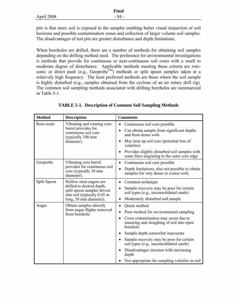
April 2008 - 84 -

Final

pits is that more soil is exposed to the sampler enabling better visual inspection of soil horizons and possible contamination zones and collection of larger volume soil samples. The disadvantages of test pits are greater disturbance and depth limitations.

When boreholes are drilled, there are a number of methods for obtaining soil samples depending on the drilling method used. The preference for environmental investigations is methods that provide for continuous or near-continuous soil cores with a small to moderate degree of disturbance. Applicable methods meeting these criteria are roto-sonic or direct push (e.g., GeoprobeTM) methods or split spoon samples taken at a relatively high frequency. The least preferred methods are those where the soil sample is highly disturbed (e.g., samples obtained from the cyclone of an air rotary drill rig). The common soil sampling methods associated with drilling boreholes are summarized in Table 5-1.

TABLE 5-1. Description of Common Soil Sampling Methods

Method Description Comments Roto-sonic Vibrating and rotating core

barrel provides for continuous soil core (typically 100 mm diameter).

• Continuous soil core possible • Can obtain sample from significant depths

and from dense soils • May heat up soil core (potential loss of

volatiles) • Provides slightly disturbed soil samples with

some fines migrating to the outer core edge Geoprobe Vibrating core barrel

provides for continuous soil core (typically 38 mm diameter).

• Continuous soil core possible • Depth limitations, also not possible to obtain

samples for very dense or coarse soils

Split Spoon Hollow stem augers are drilled to desired depth, split spoon sampler driven into soil (typically 0.45 m long, 38 mm diameter).

• Common technique • Sample recovery may be poor for certain

soil types (e.g., unconsolidated sands) • Moderately disturbed soil sample

Auger Obtain samples directly from auger flights removed from borehole.

• Quick method • Poor method for environmental sampling • Cross contamination may occur due to

smearing and sloughing of soil into open borehole

• Sample depth somewhat inaccurate • Sample recovery may be poor for certain

soil types (e.g., unconsolidated sands) • Disadvantages increase with increasing

depth • Not appropriate for sampling volatiles in soil

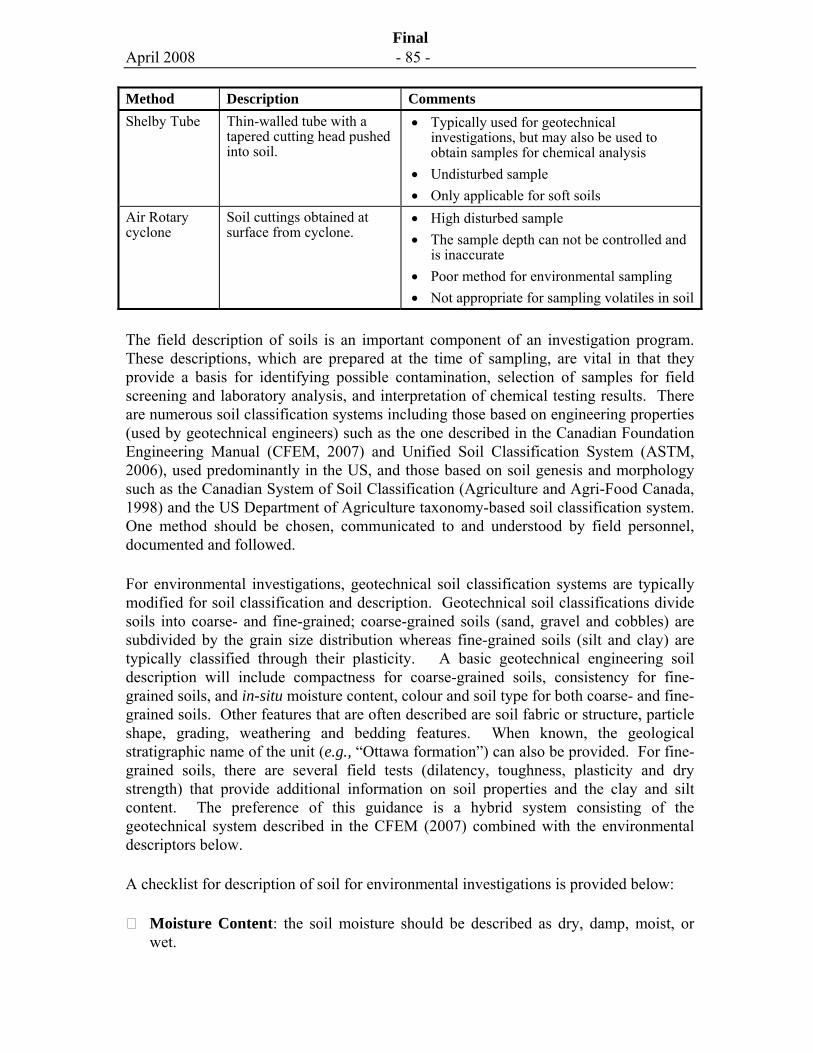
April 2008 - 85 -

Final

Method Description Comments Shelby Tube Thin-walled tube with a

tapered cutting head pushed into soil.

• Typically used for geotechnical investigations, but may also be used to obtain samples for chemical analysis

• Undisturbed sample • Only applicable for soft soils

Air Rotary cyclone

Soil cuttings obtained at surface from cyclone.

• High disturbed sample • The sample depth can not be controlled and

is inaccurate • Poor method for environmental sampling • Not appropriate for sampling volatiles in soil

The field description of soils is an important component of an investigation program. These descriptions, which are prepared at the time of sampling, are vital in that they provide a basis for identifying possible contamination, selection of samples for field screening and laboratory analysis, and interpretation of chemical testing results. There are numerous soil classification systems including those based on engineering properties (used by geotechnical engineers) such as the one described in the Canadian Foundation Engineering Manual (CFEM, 2007) and Unified Soil Classification System (ASTM, 2006), used predominantly in the US, and those based on soil genesis and morphology such as the Canadian System of Soil Classification (Agriculture and Agri-Food Canada, 1998) and the US Department of Agriculture taxonomy-based soil classification system. One method should be chosen, communicated to and understood by field personnel, documented and followed.

For environmental investigations, geotechnical soil classification systems are typically modified for soil classification and description. Geotechnical soil classifications divide soils into coarse- and fine-grained; coarse-grained soils (sand, gravel and cobbles) are subdivided by the grain size distribution whereas fine-grained soils (silt and clay) are typically classified through their plasticity. A basic geotechnical engineering soil description will include compactness for coarse-grained soils, consistency for fine-grained soils, and in-situ moisture content, colour and soil type for both coarse- and fine-grained soils. Other features that are often described are soil fabric or structure, particle shape, grading, weathering and bedding features. When known, the geological stratigraphic name of the unit (e.g., “Ottawa formation”) can also be provided. For fine-grained soils, there are several field tests (dilatency, toughness, plasticity and dry strength) that provide additional information on soil properties and the clay and silt content. The preference of this guidance is a hybrid system consisting of the geotechnical system described in the CFEM (2007) combined with the environmental descriptors below.

A checklist for description of soil for environmental investigations is provided below:

Moisture Content: the soil moisture should be described as dry, damp, moist, or wet.

April 2008 - 86 -

Final

Colour: qualitative description of colour or determined with the use of a colour chart (e.g., Munsell).

Mottles: blotches or spots of contrasting colour interspersed with the dominant soil colour.

Soil composition: this is the relative amounts of boulders, cobbles, sand, silts and clays in a soil.

Particle shape: shape of individual soil particles.

Structure or Fabric: shape of the natural soil aggregates including bedding orientation and thickness, occurrence of joints and fissures, voids, plant roots and root holes.

Debris: examples are woodwaste, metal, ash, paint flakes, clinker and asbestos; the type and approximate percentage of debris within the soil horizon should be noted.

Odour: to the extent possible describe the type of odour (e.g., diesel-like, sweet, pungent) and strength (faint, moderate, strong).

Staining: describe the colour and intensity of staining where there is evidence for discolouration caused by contamination.

Fuels or Solvents: presence of visible oil, gasoline, solvents or other organic liquids.

Compactness or consistency (optional): soil strength (coarse-grained) or degree of resistance to breaking or crushing (fine-grained).

Horizon thickness: layers of soil with distinct changes of the above features.

5.6 Field Analytical Methods

There are an emerging suite of field analytical methods that can be used to evaluate chemical concentrations in soil at contaminated sites. The field methods range from relatively simple screening tests, such as headspace vapour tests and colourimetric tests, to relatively sophisticated analyses, where equipment that provides for low-level analyses using techniques such as atomic adsorption spectrometry (AAP) or gas chromatography/mass spectrometry (GC/MS) is deployed in the field. Over the past decade, there have been significant developments in the area of sensors including x-ray fluorescence, biosensors and electrochemical detectors for metals analyses, and ultraviolet (UV) fluorescence, laser-induced fluorescence and spectrometry for organic analyses (USEPA Technology Innovation Program: Site Characterization and Monitoring Webpage http://www.epa.gov/tio/char1_tech.htm; Reible and Demnerova, 2002).

April 2008 - 87 -

Final

The objective of this section of the guidance is to describe four relatively common field techniques used for assessment of soil contamination, which are headspace vapour, colourmetric and immunoassay tests for organic compounds and x-ray fluorescence (XRF) for metals. Headspace vapour tests are the simplest field test but provide for the lowest level of quantification, whereas, colourmetric, immunoassay and XRF techniques provide for a higher level of quantification.

The potential advantages of these field analytical methods include near real-time results and potentially lower costs. Field analytical methods may be effective for follow-up phases of a site characterization program when a higher sampling density, but less precise data, is desired and acceptable, or during the site remediation phase where near real-time results can facilitate more timely and effective decision-making.

The potential disadvantages of field analytical methods include regulatory and stakeholder acceptance. An initial study involving a comparison of field methods and laboratory testing results using site samples is often required to verify the performance of the field method. The verification testing should be conducted on a sample set of sufficient size to draw statistical inferences, which generally will consist of at least 15 to 25 samples. It may also be important to conduct verification testing as a first stage pilot test and to then conduct periodic checks during the course of a field program.

Some field analytic methods require a reasonably high level of training for field personnel. It is essential that the training, quality control and testing procedures for field analytical testing be thoroughly documented.

5.6.1 Headspace Vapour Tests

Field headspace testing using detectors that measure organic vapours is a common method of screening soil samples for volatile or semi-volatile organic compounds. The procedure involves collecting a soil sample, placing it in an air-tight container (glass jar or polyethylene bag) and then analyzing the headspace vapour using a portable analytical instrument. The headspace is the air-filled part of the sample (i.e., the container is only partially filled with soil).

The recommended test procedure is as follows:

1. Fill a clean 250 to 500 ml jar half-way; a larger jar is preferred when the sampling method provides for sufficient soil.

2. Seal the jar using two sheets of aluminum foil.

3. Shake the sample jar for about ten seconds.

4. Wait between 15 and 30 minutes to allow chemicals in soil to volatilise into the headspace. If ambient temperatures are below 0oC, place the samples in a heated building or vehicle.

April 2008 - 88 -

Final

5. Puncture the seal with the probe tip and record the maximum vapour concentration measured using a field detector.

6. The headspace vapour test results should be recorded on the borehole or test pit logs.

Headspace vapour tests can be performed using either photoionisation detector (PID) with 10.2 eV or higher energy lamp, flame ionisation detector (FID) or explosimeter. For headspace vapour tests, a PID or FID may be preferred due to typically lower detection limits that can be achieved. Care must be taken when using PIDs since a positive bias may result due to moist air and/or dust being drawn into the instrument. FIDs are not sensitive to water vapour, but require a hydrogen source to operate. When using hydrogen gas, applicable regulatory requirements for transportation and storage should be followed. The instrument characteristics should be understood and instruments calibrated daily (or more frequently) in accordance with the manufacturers specifications prior to use. Typically, PIDs are calibrated using a 50 ppm or 100 ppm span gas (e.g., isobutylene). In cases where elevated VOC concentrations in ambient air could affect the calibration process, zero gas (certified clean air) should be used for “zeroing” the instrument. It is also good practice to regularly analyze a field blank consisting of moist clean soil placed in a jar that is tested using the above procedure.

The advantages of field headspace tests are it is a simple, rapid and low cost technique. The field headspace results can be used to help select samples for analytical testing. The disadvantages include that it is non-quantitative and only provides a relative indication of potential volatile or semi-volatile compound concentrations for similar soil types and contamination. Although the test is simple, it is essential that standardised procedures are consistently used and that the test methods be documented (i.e., size of jar, soil volume, equilibration time, temperature).

5.6.2 Colourimetric Tests

Method Description

Colourimetric tests refer to chemical reaction-based indicators that are used to produce compound reactions to individual compounds, or classes of compounds. Colourimetry is generally performed by mixing reagents in specified amounts with the soil sample to be tested and observing the color change in the slurry solution. The intensity of the color change is an indicator of the concentration of the chemical of interest. The color change is either observed visually through comparison with colour charts or electronically with a hand held colorimeter. Colourimetric test kits have been developed for total petroleum hydrocarbons, total PAHs and certain explosive contaminants. There are USEPA SW-846 methods for RDX and HMX in soil (Method 8510) and trinitrotoluene in soil (Method 8515) (USEPA, 1996).

April 2008 - 89 -

Final

Application

Since the detection limits are generally in the low ppm range, these field test kits are primarily used as a semi-quantitative screening tool for site characterization or to guide site remediation. The advantages of colourimetric tests are that they are relatively simple to perform and provide for near real-time results. The disadvantages with colourimetric tests include higher detection limits (depending on the kit) and possible interference by other co-contaminants, naturally occurring chemicals and organic matter. The site-specific method performance should be evaluated through comparisons between colourimetric test results and laboratory analytical results.

5.6.3 Immunoassay Tests

Method Description

Immunoassay field kits are a rapid screening tool that provide for qualitative or semi-quantitative results for specific compounds or groups of compounds. Immunoassay tests are designed to detect specific chemicals by measuring the chemicals’ response to specific antibodies. The antibodies are developed to be specific to individual compounds such as individual pesticides or chlorophenols (e.g., pentachlorophenol) or compound groups such as PAHs, PCBs or petroleum hydrocarbons. The antibodies do not respond to dissimilar substances; however, there may be cross sensitivities to compounds with similar properties. Functionally, the test is usually performed by adding a sample to a test tube coated with antibodies. A chemical is then added to the test tube that reacts with enzymes released by the antibodies. The colour change in an extracted solution in response to the enzymes is related to the specific contaminant concentration. Quantification is either determined through visual inspection or through use of a spectrophotometer.

Many immunoassay test kits have undergone significant validation (USEPA technology verification (ETV) program) and are USEPA SW-846 Methods (4000 series). There are SW-846 method immunoassay kits for the following analytes:

Analyte SW-846 Method Pentachlorophenol (PCP) 4010A 2,4 Dichlorophenoxy Acetic Acid in soil 4015 Polychlorinated Biphenyls (PCBs) in soil 4020 Total Petroleum Hydrocarbons (TPH) in soil 4030 Polynuclear Aromatic Hydrocarbons (PAH) in soil 4035 Carcinogenic PAH in soil 4035 Toxaphene in soil 4040 Chlordane in soil 4041 DDT in soil 4042 trinitrotoluene (TNT) in water and soil 4050 Hexahydro-1,3,5-Trinitro-1,3,5-Triazinc (RDX) in water and soil 4051 Triazene in water 4670

April 2008 - 90 -

Final

If properly utilized, some immunoassay tests allow for analysis of specific organics to sub-parts per million (ppm) levels in soil and sub-parts per billion (ppb) levels in water.

Applicability

The advantages of immunoassay tests are near real-time results (typically less than a 30 minute test), relatively low cost, and ability to rapidly screen a large number of samples. They are most commonly used during follow-up phases of a site characterization program when a higher sampling density is warranted or during the site remediation phase (e.g., to guide an excavation program).

The disadvantages of immunoassay tests are that the technology is not compound specific for organic chemicals such as PAHs and PCBs, and for compound specific tests for pesticides there may be cross-sensitivities to similar compounds that cause false positives. For this reason, the types of contaminants present at a site and the concentration ranges must be reasonably well known to determine if immunoassay tests are appropriate. The detection limits for immunoassay tests for some compounds are similar to conventional laboratory analyses (e.g., 0.1 to 1 ppm for PCBs for some test kits) while for other compounds are higher than laboratory detection limits. The immunoassay test process can also be sensitive to the type of matrix. For example, the test may not work well in clay soils when contaminants are strongly bound to clay particles. Immunoassay tests, although relatively simple, do require that the operator conducting the tests be adequately trained and the tests must be carefully performed to ensure accurate and repeatable results. The training, testing and quality control procedures should be documented.

5.6.4 X-ray fluorescence (XRF)

Method Description

X-ray fluorescence (XRF) is a rapid screening tool that is used to measure metal concentrations in soil. The principle behind this process is simple: when an X-ray emission from a radioactive source strikes an atom in the sample, energy is absorbed by the atom. If the energy is high enough, electrons will be displaced with the result being an x-ray with energy unique to the elements present. The x-ray emitted is detected by a fluorescence detector, which can either be a wavelength dispersive spectrometer, where the photons are separated by diffraction on a single crystal before being detected, or energy dispersive spectrometers (EDX or EDS), where the detector allows the determination of the energy of the photon when it is detected. The XRF technology is limited to certain heavy metals. Although a range of heavy metals can be simultaneously detected, there are potential cross sensitivities or interferences that may influence the accuracy and precision of the method.

April 2008 - 91 -

Final

Specific methodology has been developed by USEPA (Method 6200) to guide XRF analysis. Technology verification studies indicate the performance of XRF is variable depending on the heavy metal, matrix and instrument (USEPA, 2006b; USEPA, 2004). The detection limits generally range between 10 ppm and 500 ppm. For some metals, verification studies indicate precision and accuracy for certain XRF instruments are similar to that obtained for atomic absorption spectrometry (AAS) laboratory analysis (USEPA, 2006b). Over the past decade, advances in detector technology have improved detection limits and precision and speed of analyses using hand-held XRF detectors.

Applicability

The advantages of XRF include real-time results, when used in scanning mode on surface soil, or near real-time results when soil samples are collected and analyzed (i.e., less than 20 minutes per test) and typically lower cost than laboratory methods. The sample preparation requirements for XRF testing are relatively minimal and consist of drying and pulverising of the sample. The XRF technique is non destructive so selected samples can be sent to the laboratory for verification analysis. XRF is most commonly used during the follow-up phase of a site characterization program when contaminants of potential concern have been identified and when a higher sampling density is desired. Investigation scenarios where XRF may be employed include surface metals contamination associated with airborne deposits, paint flakes containing lead, or metals contamination associated with mining or mineral-processing wastes.

The disadvantages of XRF include higher detection limits than laboratory analyses and possible cross-sensitivities for certain heavy metals. The soil matrix and moisture can influence results, although this can be improved through drying, sieving and milling or pulverising the sample. It is generally advisable to perform a pilot test where split samples are analyzed using XRF and laboratory methods. Persons using XRF detectors must have appropriate certification and training for radiation-emitting equipment.

5.7 Field Preservation of Soil Samples for VOC Analysis

Sample collection, handling and storage procedures have been shown to have a significant influence on soil analytical results for volatile organic compounds. Unless appropriate procedures are used, there can be substantial losses and negative bias introduced through volatilisation and biodegradation. Of particular importance are whether field preservation methods or specialized sampling devices are used, since numerous studies comparing analytical concentrations for samples collected using conventional containers without field preservation to those that were either field preserved or collected using specialized devices and then rapidly preserved when received by the laboratory indicate a consistent negative bias typically ranging between 50 and 90 percent (Minnich et al., 1997; Ball et al., 1997; USEPA, 1997; Hewitt, 1999; Sorini et al., 2002).

April 2008 - 92 -

Final

As a result over the concern with negative bias for volatile organic analyses, USEPA published methods 5035 and 5021 (USEPA, 1997), which include requirements for field preservation immediately upon sample collection using either methanol or sodium bisulfate or use of a specialized air-tight vial (e.g., EncoreTM sampler), which is extracted and preserved upon receipt by the laboratory. The American Society for Testing and Materials (ASTM) Method 4547-98 “Standard Guide for Sampling Wastes and Soil for Volatile Organic Compounds” also addresses requirements for field preservation. Numerous other regulatory agencies have also adopted protocols for field preservation (New Jersey Department of Environmental Protection, 1997; Massachusetts Department of Environmental Protection, 1999; California Regional Water Quality Control Board, 1999).

The preservation of soil samples in the field or sampling using specialized containers with laboratory preservation within 48 hours of sample collection, in accordance with USEPA Method 5035 or 5021 or similar method, is recommended for analysis of volatile organic compounds in soil. Deviations from standard protocols should be identified together with supporting rationale.

5.8 Data Validation and Interpretation

Data validation and interpretation are essential components of the site investigation process. Data validation was discussed in Chapter 2, and a checklist is provided in Volume 2. The focus of this section is data interpretation and statistical analysis for characterization of soil quality.

Exploratory data views should be completed (Chapter 2) and basic statistical parameters should be calculated for each data set (ProUCL is a useful software tool for this purpose; see Section 5.9). When a dataset represents a single population, a statistical evaluation of soil quality is justified. There are a number of approaches that may be used to evaluate population characteristics of a data set including a review of historical information and contaminant migration characteristics and the statistical techniques described below. Soil that has become contaminated by similar processes and events will likely have contamination concentrations that represent a single population. If sampling is limited to judgmental sampling, the statistical analyses described below may not be appropriate.

5.8.1 Evaluation of Data Distributions

The statistical tests that can be used to evaluate data populations and distributions include:

Frequency Distributions and Histograms: These techniques can be used to evaluate whether there is the potential for multiple populations. For example, a large gap in a frequency distribution plot may indicate separate populations.

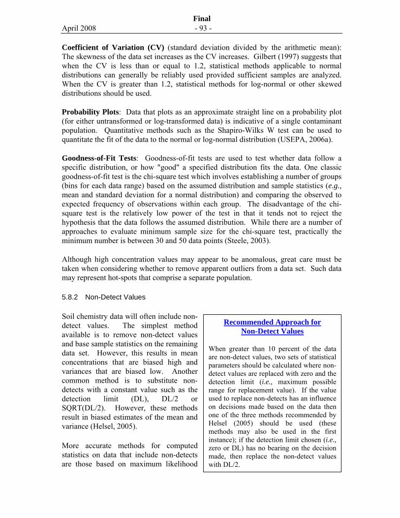
April 2008 - 93 -

Final

Coefficient of Variation (CV) (standard deviation divided by the arithmetic mean): The skewness of the data set increases as the CV increases. Gilbert (1997) suggests that when the CV is less than or equal to 1.2, statistical methods applicable to normal distributions can generally be reliably used provided sufficient samples are analyzed. When the CV is greater than 1.2, statistical methods for log-normal or other skewed distributions should be used.

Probability Plots: Data that plots as an approximate straight line on a probability plot (for either untransformed or log-transformed data) is indicative of a single contaminant population. Quantitative methods such as the Shapiro-Wilks W test can be used to quantitate the fit of the data to the normal or log-normal distribution (USEPA, 2006a).

Goodness-of-Fit Tests: Goodness-of-fit tests are used to test whether data follow a specific distribution, or how "good" a specified distribution fits the data. One classic goodness-of-fit test is the chi-square test which involves establishing a number of groups (bins for each data range) based on the assumed distribution and sample statistics (e.g., mean and standard deviation for a normal distribution) and comparing the observed to expected frequency of observations within each group. The disadvantage of the chi-square test is the relatively low power of the test in that it tends not to reject the hypothesis that the data follows the assumed distribution. While there are a number of approaches to evaluate minimum sample size for the chi-square test, practically the minimum number is between 30 and 50 data points (Steele, 2003).

Although high concentration values may appear to be anomalous, great care must be taken when considering whether to remove apparent outliers from a data set. Such data may represent hot-spots that comprise a separate population.

5.8.2 Non-Detect Values

Soil chemistry data will often include non-detect values. The simplest method available is to remove non-detect values and base sample statistics on the remaining data set. However, this results in mean concentrations that are biased high and variances that are biased low. Another common method is to substitute non-detects with a constant value such as the detection limit (DL), DL/2 or SQRT(DL/2). However, these methods result in biased estimates of the mean and variance (Helsel, 2005).

More accurate methods for computed statistics on data that include non-detects are those based on maximum likelihood

Recommended Approach for Non-Detect Values

When greater than 10 percent of the data are non-detect values, two sets of statistical parameters should be calculated where non-detect values are replaced with zero and the detection limit (i.e., maximum possible range for replacement value). If the value used to replace non-detects has an influence on decisions made based on the data then one of the three methods recommended by Helsel (2005) should be used (these methods may also be used in the first instance); if the detection limit chosen (i.e., zero or DL) has no bearing on the decision made, then replace the non-detect values with DL/2.

April 2008 - 94 -

Final

estimation methods (Cohen, 1959; Cohen, 1961; Helsel, 2005) or those based on computational methods where varying values are assigned to non-detect data based on fitting the data to a probability plot either using graphical methods or regression analysis. This method assumes that the distribution of the data above and below the detection limit is the same. Gilbert (1987) advices against using this method when there is greater than 15 percent non-detects, unless the distribution is known to be log-normal.

Helsel (2005) summarizing a number of studies indicates that the traditional method of replacing the non-detect values with half the detection limit can result in a significant bias when more than 10 percent of data are non-detect values and recommends one of three methods for dealing with non-detect values (i) maximum likelihood estimation, (ii) imputation methods, and (iii) the Kaplan-Meier method.

5.8.3 Statistical Characterization of Soil Data

For investigations where the sampling design supports the statistical analyses of data (e.g., random and systematic grid sampling) and where the distribution analysis above supports a single population, a statistical approach may be adopted to characterize a defined volume of soil for comparison to regulatory criteria. The soil volume is considered to meet the regulatory criteria when:

• the data is demonstrably representative of one population; and, for that data set;

• the upper 90th percentile of the sample concentrations is less than the criterion concentration;

• the upper 95 percent confidence limit of the arithmetic mean concentration of the samples is less than the criterion concentration; and,

• step-out sampling for any sample, which had a concentration exceeding two times the criterion concentration, has confirmed that the exceedance is random and localized (e.g., none of the step-out samples had concentrations exceeding the criterion).

For a CV less than or equal to 1.2, statistical methods applicable to normal distributions may be used. For a CV greater than 1.2, statistical methods for log-normal or other skewed distributions should be used (Gilbert, 1987; USEPA, 2002).

Locations where a sample concentration exceeds two times the applicable criterion, should generally be subjected to delineation (“step-out”) sampling to establish whether the exceedance represents a larger “hot-spot” area of contamination or whether it represents a single random exceedance that belongs to the data population. Based on the sample spacing defined in Exhibit 5.2, a hot-spot is an area of contamination that is larger than approximately 5 m to 10 m in horizontal extent, and 0.5 m to 1 m in vertical extent.

April 2008 - 95 -

Final

The step-out sampling described above may result in sampling bias due to locally higher sampling density and multiple sampling locations that are spatially correlated (i.e., not independent). Statistical procedures that assume independent and approximately randomly distributed concentrations are not appropriate for correlated data. To remove the bias, sampling locations may be selectively excluded, thus creating a non-correlated data set for statistical analysis. Possible spatial correlation may be evaluated using geostatistical programs such as Spatial Analysis and Decision Assistance (SADA) software (see Section 5.9 for an additional description). To discern whether there are correlations, a variogram function versus lag distance plot may be calculated for various lag distances, data search orientations and variogram estimators.

5.8.4 Comparison of Population Means

For some investigations, it may be important to compare data for an area of potential concern to those representing background concentrations. A method is provided below for evaluating whether two population means are significantly different, which is robust and intuitive for data sets that have unequal sample sizes. Upper and lower confidence limits (UCLM and LCLM) of the difference between two population means are calculated as follows:

2

22

1

21

2/21 )(LCLMns

ns

txx +−−= α [5.3]

2

22

1

21

2/21 )(ns

nstxxUCLM ++−= α [5.4]

where 1x and 21s , and 2x and 2

2s are the means and variances and 1n and 2n are the samples sizes, respectively, from approximate normal distributions, and 2/αt (where α=0.1) is the value of the t-distribution with v degrees of freedom (leaving an area of α/2 to the right):

)]1/()/[()]1/()/[()//(

22

2221

21

21

22

221

21

−+−+

=nnsnns

nsnsv [5.5]

If the confidence limit brackets zero, the two populations likely represent the same population at an acceptable level of confidence. More importantly, the confidence interval also provides information for deciding whether the magnitude of the mean difference is tolerable to the decision maker or not. For example, if the confidence limit brackets zero at a significance level of 0.1, one could be 90 percent confident that the confidence limit contains the true difference between the means. Therefore, one could consider the means of the two data sets to be statistically similar.

April 2008 - 96 -

Final

5.8.5 Data Presentation and Reporting

Soil characterization reports should include tabulated data on tables and figures as a means to convey relevant information to the reader. Since often soil and groundwater data are presented together, a more detailed description of data presentation format is provided in Chapter 6. Essential items for presentation and reporting of soil data are:

• Tabulate all data including sample location, sample identifier, sample date, sample depth, sampling methods, chemical analysis methods, laboratory detection limits and results of chemical analysis;

• Tabulate field screening and laboratory analysis data to enable side-by-side comparisons; and,

• Provide detailed descriptions of stratigraphy and indicators of potential contamination (e.g., staining, debris) and field screening tests (e.g., headspace tests) on borehole and test pit logs.

It is also often helpful to show soil concentration data on plans to illustrate the spatial distribution in concentrations.

5.9 Resources and Weblinks

Over the last decade a number of software tools, often described as Decision Support Software (DSS), have been developed to support site investigation planning, analysis of data and a structured decision-making process for environmental management decisions. A review by USEPA indicates over 50 different tools have been developed addressing a wide range of decision support areas including site characterization data analysis and visualisation, data worth analysis, option analysis using decision analysis tools, remediation technology selection, human health risk assessment, and economic and cost/benefit analysis. The new software provide capabilities in the area of visually-based development of sampling plans, rapid processing and integration of spatial information and contaminant data as it is obtained, and two- and three-dimensional contouring and visualization of data. The software tools represent varying levels of sophistication in terms of statistical design and analysis methods. Some software tools include a human health risk assessment module where potential exposure and risk associated with measured concentration data can be evaluated. While these tools are potentially useful for assessment and management of contaminated sites, the assumptions and limitations of the statistical models should be understood. Care must be taken to appropriately match the capabilities of the tool with the problem under consideration. For some types of software tools (e.g., 3-D visualisation using geostatistical methods), a significant quantity of data is required, which may be infrequently available at contaminated sites.

April 2008 - 97 -

Final

Spatial Analysis Decision Assistance (SADA): A software program developed by the University of Tennessee Research Corporation for USEPA that integrates a number of tools for data visualization, statistical analysis, decision analysis and human health and ecological risk assessment. The modules that are part of SADA are data exploration: statistical summaries, database query, data screening relative to thresholds; data visualization: two-dimensional slices and three-dimensional volumes; geospatial analysis: tools for measuring spatial correlation among data, interpolation routines including kriging, inverse distance, nearest neighbour and contouring programs; human health risk assessment: estimation of risk following Risk Assessment Guidance for Superfund (RAGS); decision analysis: summarization, visualization, and modeling tools to aid decision making; cost benefit analysis: site-specific cost-benefit curves for given remedial cleanup goal; and secondary sampling: different strategies for determining future sampling locations (www.tiem.utk.edu/~sada/).

Field Environmental Decision Support (FIELDS): An ArcView® compatible software program developed by USEPA that combines a geographic information system (GIS) interface, global positioning system (GPS), database and imaging technologies to help process, assess and communicate environmental data. The software includes the capability through global positioning technology and a direct link to the output of supported field detectors (e.g., PIDs and XRFs from certain manufacturers) to plot a two-dimensional display of the data in real-time over an aerial photograph or site map. The data can be processed as it is obtained through programs than enable statistical parameters to be calculated, measurements to be compared to a specified threshold, or contouring of data using a natural neighbor interpolation algorithm. There are also trend analysis windows that show changes in collected data values over time. A human health and ecological module is also available (www.epa.gov/region5fields/).

Visual Sampling Plan (VSP): A software tool designed to assist in sampling plan design for site characterization developed by the U.S. Department of Energy (DOE) Pacific Northwest National Laboratory. VSP is designed to select the number of samples needed to satisfy specified criteria and develop two-dimensional sampling designs that may be overlain on site maps. The tool may be used to construct a sampling grid based on a systematic design or statistically-based designs such as random or stratified random sampling or hot-spot sampling designed to detect a certain size source with a defined probability (i.e., Section 5.3.4). The number of samples can be determined through statistical hypothesis testing to meet defined decision criteria through comparison of mean or percentiles to acceptable threshold values (i.e., Section 5.3.4). A module for in-fill sampling based on largest spacing between samples is also provided. (http://dqo.pnl.gov/vsp)

Paraview: Paraview is a visualization, not modelling, program that uses 2-D and 3-D geometric points as input data. Multiple scalar, vector and colour properties can be attached to the points. Data filters are then applied to create sections, contours, extrusions, warping, etc. In addition, datasets can be manipulated using a built-in calculator filter. Colour-mapping and transparency are two of the many effects available. Graphic output can include: animations by viewpoint and/or parameters in

April 2008 - 98 -

Final

MPG and AVI formats; screen-capture of still images in JPG and BMP and PNG formats; postscript for very high resolution; and, direct to printer. Data output options include transformed datasets. The program can create ASCII session files that record the current state of model creation, that can be edited by hand, and that are used as scripts in restoring the model at a later time or publishing the model to other users. The development of Paraview is ongoing, at Kitware, Inc. and U.S. national laboratories in Los Alamos, Sandia and Lawrence Livermore. The intent is to create an open-source, scalable, parallel processing and distributed memory program that is freely available. Development is being funded by U.S. Dept. of Energy. (http://www.paraview.org/HTML/Screenshots.html)

Surfer: A commercial program available at relatively low cost, Surfer is a highly capable program for contouring, gridding, surface mapping and other similar analyses, using many different customizable algorithms. Input data is in the format of (X,Y,parameter), from which the program can create labeled and coloured 2-D and 3-D plots of the output as linework and continuous bitmapped images, AutoCAD DXF files and grid files in binary or ASCII format for input to other programs. (http://www.goldensoftware.com/products/surfer/surfer.shtml)

Voxler: A commercial program available at relatively low cost, Voxler is similar to Paraview in capabilities, although some specific attributes are different. For example, Voxler is more limited in the complexity of the datasets it can handle, while it is much enhanced in most aspects of colour-mapping. Its user interface adheres more closely to the MS Windows standard than Paraview’s. Voxler has been created by the same company that produces Surfer, and can use as input the grid files output by Surfer. Choosing which of the two (Paraview or Voxler) to use for a particular project depends on the input data and on the desired output result. (http://www.goldensoftware.com/products/voxler/voxler.shtml)

The USEPA Field Analytic Technologies database provides information of latest advances in field methods including technologies such as field gas chromatographic methods, immunoassay test kits, laser-induced fluorescence, X-ray fluorescence, direct push methods, soil and soil gas samples, passive diffusion bags for sampling groundwater. http://clu-in.org/char/technologies/

The USEPA ProUCL free software calculates summary statistics, performs goodness-of-fit testing to evaluate whether data follows a normal or log-normal distribution and calculates the upper confidence of the mean using a number of parametric and non-parametric methods. http://www.epa.gov/nerlesd1/tsc/software.htm

April 2008 - 99 -

Final

5.10 REFERENCES

Agriculture and Agri-Food Canada Publication, 1988. The Canadian System of Soil Classification, 3rd ed. 1646, 187 pp.

American Society for Testing and Materials Standards (ASTM) D2487-06, 2006. Standard Classification of Soils for Engineering Purposes (Unified Soil Classification System), 12 pages.

Ball, W.P., G. Xia, D.P. Durfee, R.D. Wilson, M.J.Brown and D.M. Mackay. 1997. Hot Methanol Extraction for the Analysis of Volatile Organic Chemicals in Surface Core Samples for Dover Air Force Base, Delaware. Ground Water Monitoring and Remediation, Winter, pg. 104-121.

British Columbia Ministry of Environment, 2005a. Technical Guidance 12 on Contaminated Sites: Statistics for Contaminated Sites.

British Columbia Ministry of Environment, 2005b. Technical Guidance 1 on Contaminated Sites: Site Characterization and Confirmation Testing.

CFEM (Canadian Foundation Engineering Manual), 2007. 4th Edition, Bitech Publishers Ltd.

California Regional Water Quality Control Board (CRWQB), 1999. Fact Sheet Underground Storage Tank (US) Program (2/1/99).

Cohen, A.C. 1959. Simplified estimators for the normal distribution when samples are singly censored or truncated. Technometrics 1:217-237

Cohen, A.C. 1961. Tables for maximum likelihood estimates: singly truncated and singly censored samples. Technometrics 3:535-541.

Gilbert, R. O., and P. G. Doctor. 1985. Determining the Number and Size of Soil Aliquots for Assessing Particulate Contaminant Concentrations. Journal of Environmental Quality. Vol. 14: 286-292.

Gilbert, R.O. 1987. Statistical Methods for Environmental Pollution Monitoring. Van Nostrand Reinhold Company, New York, NY. 320 pp.

Hardin, J.W., and R.O. Gilbert, 1993. Comparing Statistical Tests for Detecting Soil Contamination Greater than Background, Report to U.S. Department of Energy, PNL-8989, UC-630, Pacific Northwest Laboratory, Richland, WA.

Helsel, D. 2005. More than Obvious: Better Methods for Interpreting Nondetect Data. Environ. Science and Technol. 39 (20): 409A-424A.

April 2008 - 100 -

Final

.

Hewitt, A.D. 1999. Storage and Preservation of Soil Samples for Volatile Compounds Analysis. Report prepared for US Army Corp of Engineers. May.

Hirotaka, S. and P. Goovaerts. 2001. Accounting for source location and transport direction into geostatistical prediction of contaminants. Environ. Sci. Technol. 35 (24): 4823-4829.

Massachusetts Department of Environmental Protection, 1999. Preservation Techniques for Volatile Organic Compound (VOC) Soil Sample Analyses, Commonwealth of Massachusetts, Report WSC # 99-415.

Minnich, M.M, B.A. Schumacher and J.H. Zimmerman. 1997. Comparison of Soil VOCs Measured by Soil Gas, Heated Headspace, and Methanol Extraction Techniques. J. Soil Contam. 6(2); 187-203.

New Jersey Department of Environmental Protection, 1997. Methanol Preservation/Extraction of Soil Samples: Policy Implementation Guidance, Memorandum from Richard Gimello, Assistant Commissioner, July 1.

Ott, W.R. 1990. A Physical Explanation of the Lognormality of Pollutant Concentrations, J.Air Waste Manag Assoc, 40: 1378.

Ott, W.R. 1995. Environmental Statistics and Data Analysis, Lewis Publishers, Boca Raton, FL.

Reible, D. and K. Demnerova (Editors), 2002. Innovative Approaches to the On-Site Assessment and Remediation of Contaminated Sites, Kluwer Academic Publishers, Boston.

Sorini, S.S., J.F. Schabron and J.F. Rovani, 2002. Evaluation of VOC Loss from Soil Samples: Extrusion into Empty VOA Vials, Refrigerated Storage and Methanol Injection in Preparation for Volatile Organic Analysis. AEHS Soil, Sediment and Water Magazine of Environmental Assessment and Remediation, April/May Edition.

Steele, M.C. 2003. The Power of Categorical Goodness-of-Fit Statistics. Ph.D. thesis. Griffith University, Australia. http://www4.gu.edu.au:8080/adt-root/public/adt-QGU20031006.143823/index.html

U.S. Environmental Protection Agency, 2006a. Data Quality Assessment: Statistical Methods for Practitioners EPA QA/G-9S. Washington, DC. Report EPA/24/B-06/003. February.

April 2008 - 101 -

Final

U.S. Environmental Protection Agency, 2006b. Innovative Technology Verification Report XRF Technologies for Measuring Trace Elements in Soil and Sediment Oxford X-Met 3000TX XRF Analyzer, EPA/540/R-06/008 Washington, DC 20460, February.

U.S. Environmental Protection Agency, 2004. Field Measurement Technology for Mercury in Soil and Sediment, NITON’s XLi/XLt 700 Series X-Ray Fluorescence Analyzers. Office of Research and Development, Washington, D.C. Report EPA/600/R-03/148, May.

U.S. Environmental Protection Agency, 2002. Guidance on Choosing a Sampling Design for Environmental Data Collection for Use in Developing a Quality Assurance Project Plan, Washington, DC 20460. EPA QA/G-5S, December

U.S. Environmental Protection Agency, 1997. Test Methods for Evaluating Solid Waste, No. SW846, Final Update III, Method 5035, June 13.

U. S. Environmental Protection Agency, 1996. Project Summary Field Sampling and Sampling On-Site Analytical Methods for Explosives in Soil. EPA/540/S-97/501, December.

U. S. Environmental Protection Agency, 1994. Methods for Evaluating the Attainments of Cleanup Standards: Volume 3: Reference-Based Standards. EPA/230/R-94-004. Office of Policy, Planning, and Evaluation. (NTIS: PB94-176831)

U. S. Environmental Protection Agency, 1992. Methods for Evaluating the Attainments of Cleanup Standards: Volume 2: Ground Water. EPA/230/R-92/014. Office of Policy, Planning, and Evaluation. (NTIS: PB94-138815)

U. S. Environmental Protection Agency, 1989a. Methods for Evaluating the Attainments of Cleanup Standards: Volume 1: Soils and Solid Media. EPA/230/02-89-042. Office of Policy, Planning, and Evaluation. (NTIS: PB89-234959)

USPEA, 1989b. Soil Sampling Quality Assurance User’s Guide, 2nd Edition. Report EPA/600/8-89/046, March.

April 2008 - 102 -

Final

APPENDIX 5-1: Confirmation of Remediation Soil Sampling

This appendix provides guidance on sampling design for confirmation of remediation where soil contamination has been excavated at a site. The remedial excavation process often will involve the use of screening-level field analytical testing described in Chapter 5; however, at the completion of remediation, confirmatory samples are generally analyzed using laboratory methods to verify whether or not remediation objectives have been met. During the site remediation process, excavated soil is often placed in stockpiles to facilitate segregation and characterization for soil management.

The site remediation process requires consideration of numerous aspects that go beyond the scope of this guidance. The scope of this appendix is limited to confirmatory sampling design for remedial excavation programs and stockpile soil characterization. While specific guidance is provided below on sampling frequency and spacing, as described elsewhere in the guidance, there may be alternate sampling designs that are acceptable and that meet project objectives. Any deviations from the guidance provided in this appendix should be documented and a rationale should be provided.

A5.1 SAMPLING DESIGN - CONFIRMATION OF REMEDIATION

Following completion of a remedial excavation program, samples from the excavation should be obtained and analyzed to confirm that contamination was removed. The minimum requirements for confirmation of remediation sampling are:

• Discrete samples should be collected from each excavation face (i.e., walls and base);

• One discrete confirmatory sample should be collected and analyzed such that there is at least one sample within a grid based on 10-m increments (5-m increments for hazardous waste);

• More closely spaced confirmation sampling may be necessary where there are thin identifiable soil layers that are suspected to be contaminated; and

• Samples should be collected from within a 0.2 m perpendicular distance from the excavation surface.

Depending on the type of contamination, field screening methods may be used to target samples for chemical analysis. Several field screening methods are described below.

For confirmation of non-hazardous waste remediation, up to four discrete soil samples may be composited. However, the concentration in the composite soil sample should be compared to the applicable regulatory criterion divided by four. It is recommended that all the discrete soil samples be analyzed if the composite concentration exceeds the adjusted regulatory criterion.

April 2008 - 103 -

Final

If concentrations in the confirmatory soil samples exceed the regulatory criteria, additional soil should be excavated and the above process should be repeated, unless an alternate approach (e.g., risk management or in situ treatment) is followed.

A 5.2 SAMPLING DESIGN - EX SITU (STOCKPILE) CHARACTERIZATION

Stockpile sampling may be used to characterize contaminant levels in soils, excavated at a contaminated site, that are to be disposed of off site or treated. While the details of stockpile sampling will vary depending on project specific objectives and requirements and possible regulatory constraints, the approach for stockpile characterization should follow certain principles, as described below.

Stockpile sampling should not be used as a means to characterize a site; the site should be adequately characterized using in situ sampling.

Soil should be segregated during the excavation process and placed in separate like stockpiles that correspond to the inferred contamination level based on prior knowledge from in situ characterization, field screening and analytical testing, and where applicable, visual and/or olfactory indications of potential contamination. For example, soil at a site could be segregated into three classes consisting of soil most likely to be contaminated, suspected to be contaminated, and likely to be not contaminated.

The stockpile soil volume will depend on the contamination level; typically, a larger stockpile size is acceptable for soil with low levels of contamination while a smaller stockpile is warranted when contamination levels are higher (e.g., hazardous waste). The size may also depend on the contaminant type, toxicity, disposal or treatment costs, or other practical considerations.

The stockpile sampling design will depend on the contaminant characteristics. For sampling purposes, stockpiles are divided into equal-volume cells. For volatile organic contaminants, two co-located discrete samples are obtained from each cell. A field headspace test is conducted on each co-located discrete sample. Samples are selected for laboratory analysis on the basis of the headspace test results and visual/olfactory indications of potential contamination. The analytical testing program is often biased toward samples inferred to have the greatest potential for contamination. For non-volatile contaminants, the typical approach is a sampling progression that begins with collection of several small-scale aliquots that are combined together to form a discrete sample. The discrete sample from each cell is split into two sub-samples and a composite sample is formed from the discrete sub-samples that are mixed.

The sampling locations should provide for uniform sample collection from the soil stockpile. Collection of soil samples from the surface of the stockpile is not acceptable; instead a method that provides for samples within the core of the stockpile should be employed. Care must be exercised to ensure that a discrete sample is made up of equal parts (equal volumes) of the aliquots collected.

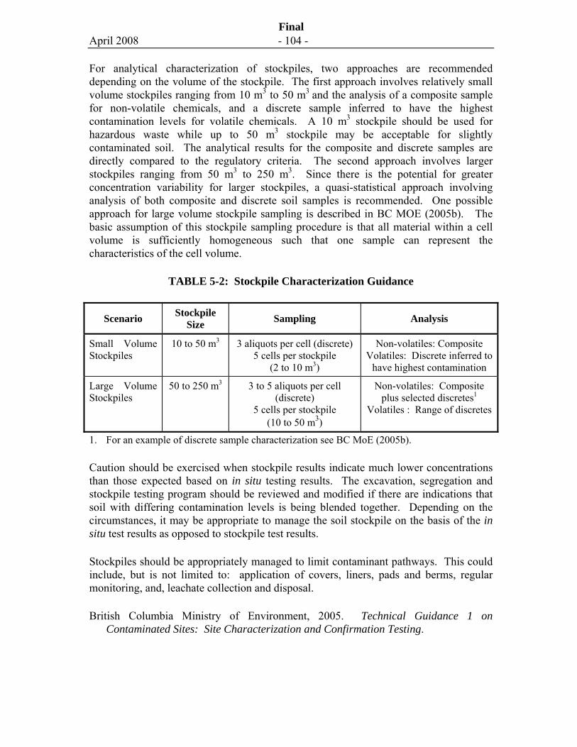
April 2008 - 104 -

Final

For analytical characterization of stockpiles, two approaches are recommended depending on the volume of the stockpile. The first approach involves relatively small volume stockpiles ranging from 10 m3 to 50 m3 and the analysis of a composite sample for non-volatile chemicals, and a discrete sample inferred to have the highest contamination levels for volatile chemicals. A 10 m3 stockpile should be used for hazardous waste while up to 50 m3 stockpile may be acceptable for slightly contaminated soil. The analytical results for the composite and discrete samples are directly compared to the regulatory criteria. The second approach involves larger stockpiles ranging from 50 m3 to 250 m3. Since there is the potential for greater concentration variability for larger stockpiles, a quasi-statistical approach involving analysis of both composite and discrete soil samples is recommended. One possible approach for large volume stockpile sampling is described in BC MOE (2005b). The basic assumption of this stockpile sampling procedure is that all material within a cell volume is sufficiently homogeneous such that one sample can represent the characteristics of the cell volume.

TABLE 5-2: Stockpile Characterization Guidance

Scenario Stockpile Size Sampling Analysis

Small Volume Stockpiles

10 to 50 m3 3 aliquots per cell (discrete)5 cells per stockpile

(2 to 10 m3)

Non-volatiles: Composite Volatiles: Discrete inferred to

have highest contamination

Large Volume Stockpiles

50 to 250 m3 3 to 5 aliquots per cell (discrete)

5 cells per stockpile (10 to 50 m3)

Non-volatiles: Composite plus selected discretes1

Volatiles : Range of discretes

1. For an example of discrete sample characterization see BC MoE (2005b).

Caution should be exercised when stockpile results indicate much lower concentrations than those expected based on in situ testing results. The excavation, segregation and stockpile testing program should be reviewed and modified if there are indications that soil with differing contamination levels is being blended together. Depending on the circumstances, it may be appropriate to manage the soil stockpile on the basis of the in situ test results as opposed to stockpile test results.

Stockpiles should be appropriately managed to limit contaminant pathways. This could include, but is not limited to: application of covers, liners, pads and berms, regular monitoring, and, leachate collection and disposal.

British Columbia Ministry of Environment, 2005. Technical Guidance 1 on Contaminated Sites: Site Characterization and Confirmation Testing.

April 2008 - 105 -

Final

6.0 GROUNDWATER CHARACTERIZATION GUIDANCE

6.1 Purpose, Background and Need

In Canada, groundwater is a commonly used and valued resource. Protective criteria have been developed for various groundwater uses, including drinking water, irrigation, and livestock watering, as well as criteria to protect aquatic life in water bodies that may receive groundwater. To serve their intended purpose, it is important that groundwater criteria are applied against accurate and reliable groundwater quality data that have been acquired in a manner that represents, as best as practical, the quality of the groundwater source (i.e., the aquifer) and the manner in which the water is extracted (e.g., withdrawals from small domestic wells versus large municipal production wells).

Many groundwater investigation programs at contaminated sites fall short of their objectives because the data obtained are not representative, and are subsequently relied upon inappropriately for the assessment of risks and/or the design of a remedial system. The purpose of this groundwater guidance is to describe the approach and methods for acquiring representative data that should be considered when undertaking site characterization programs at contaminated sites where the information obtained is to be used to evaluate potential human health risk from groundwater consumption or use. Appropriate groundwater characterization may be achieved through the completion of a detailed background information review (as discussed in Chapter 2) and a focused field program that obtains site data at a scale that is compatible with the scale required in order to make decisions on actual risk. The uncertainties in the data set must be understood and tolerable, and communicated effectively to the risk assessor, who may then factor these uncertainties into their own assessment. For purposes of this guidance, emphasis is placed on acquiring representative data at the appropriate scale. In this context, scale is taken to mean the:

a) spatial scale (vertical and horizontal distribution of contaminants in the subsurface) at a site that is compatible with the scale at which groundwater withdrawals occur, yielding concentrations of a contaminant that may be encountered by a receptor (e.g., concentrations in groundwater at the well head of a water supply well),

Groundwater Characterization

This chapter describes the planning, process and methods for groundwater characterization. The key elements and their corresponding sections in the chapter are:

Conceptual site model development (6.2),

Approach and sampling design (6.3),

Acquiring hydrogeologic information and monitoring networks (6.4 and 6.5),

Field and laboratory data acquisition (6.6),

Well abandonment (6.7), and

Data assessment, interpretation and presentation (6.8 and 6.9).

Related tools are Suggested Operating Procedures for Low-Flow Groundwater Sampling (SOP-2) and Borehole Drilling and Monitoring Well Installation (SOP-3).

April 2008 - 106 -

Final

b) chemical scale, in terms of the range of chemicals of concern to be analysed, including their possible transformation products and their respective detection limits, all of which should be considered in the risk assessment, and

c) temporal scale that provides certainty, within tolerable limits, of the expected concentrations that may be encountered over time at a receptor.

Temporal scales may include both short-term concentration variations caused, for example, by tidal changes in water-level elevations, seasonal changes in elevation and/or groundwater flow direction, and longer-term trends (e.g., over several years) in chemical or hydrogeological conditions.

6.1.1 Obtaining Representative Samples from the Well

Rigorous and accepted groundwater sampling procedures are available and commonly used by groundwater practitioners to acquire samples that are considered to be representative of actual groundwater conditions (refer to Section 6.6.2 and Volume 2). However, when the hydraulic characteristics of the aquifer and the physical process of water movement from the aquifer to the well screen are closely examined, then it becomes apparent that most groundwater sampling procedures, including those that purport to minimize sampling bias, may yield high quality samples that are not truly representative of the aquifer. Rather, and as discussed further below, the samples are more likely to represent a quasi-average of actual conditions, and the concentrations in the samples can often be biased low because of an averaging effect.

If the concentrations of a particular contaminant were the same throughout the aquifer of interest, then the problem of obtaining representative samples would be greatly simplified; there would be no need to consider the length of a monitoring well screen when designing a monitoring program, provided that the well was completed somewhere within the aquifer. All samples acquired using similar procedures would yield very similar results, with variances mainly attributable to sampling technique, changes occurring during sample storage, transport and handling prior to analysis, and variance introduced by the analytical procedures.

In reality, such variances are often overshadowed by the variance introduced because of the heterogeneous distribution of contaminants within the aquifer. For example, in impacted aquifers, it is common to encounter varying concentrations of contaminants at different depths within the aquifer. Concentrations may vary by orders-of-magnitude over vertical distances of only a few centimetres (e.g., Pitkin et al., 1999). As illustrated in Figure 6-1, when such variations in concentration are present in the geologic formation adjacent to a length of well screen, then sampling will result in mixing at the well. In heterogeneous aquifers such as the multi-layered system shown, each soil type may carry a different concentration, Ci, of the same dissolved chemical species. When the well is pumped, a sample of the pumped water will represent a quasi-average, CSAMPLE, of the concentrations in each layer.

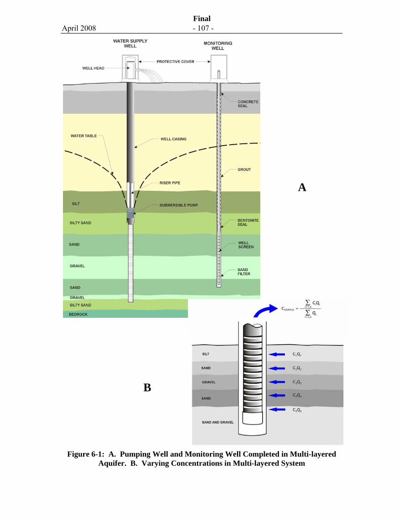
April 2008 - 107 -

Final

Figure 6-1: A. Pumping Well and Monitoring Well Completed in Multi-layered Aquifer. B. Varying Concentrations in Multi-layered System

A

B

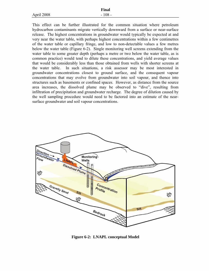
April 2008 - 108 -

Final

This effect can be further illustrated for the common situation where petroleum hydrocarbon contaminants migrate vertically downward from a surface or near-surface release. The highest concentrations in groundwater would typically be expected at and very near the water table, with perhaps highest concentrations within a few centimetres of the water table or capillary fringe, and low to non-detectable values a few metres below the water table (Figure 6-2). Single monitoring well screens extending from the water table to some greater depth (perhaps a metre or two below the water table, as is common practice) would tend to dilute these concentrations, and yield average values that would be considerably less than those obtained from wells with shorter screens at the water table. In such situations, a risk assessor may be most interested in groundwater concentrations closest to ground surface, and the consequent vapour concentrations that may evolve from groundwater into soil vapour, and thence into structures such as basements or confined spaces. However, as distance from the source area increases, the dissolved plume may be observed to “dive”, resulting from infiltration of precipitation and groundwater recharge. The degree of dilution caused by the well sampling procedure would need to be factored into an estimate of the near-surface groundwater and soil vapour concentrations.

Figure 6-2: LNAPL conceptual Model

April 2008 - 109 -

Final

A further and probably more important complication arises where the aquifer is not homogeneous (i.e., the hydraulic properties of the aquifer are not the same, but vary with location in the aquifer) and is anisotropic (i.e., the hydraulic properties vary depending on the direction in which they are measured). In such aquifers, relatively long monitoring well screens are likely to intercept different zones of higher and lower permeability, some of which may be highly contaminated and some not. Where commonly accepted sampling protocols are applied, the average concentrations obtained at a monitoring well in such a system will be biased towards concentrations in the more permeable zones. At one extreme, even though an aquifer may be highly contaminated, permeable zones that are relatively free of contamination may result in well water samples that contain little of the contaminants. At the other extreme, a relatively clean aquifer with contamination that occurs in one or two thin permeable units may yield high concentrations at the well that do not necessarily represent the overall condition of the aquifer or the water quality that can be expected at a water supply well or in a groundwater discharge zone beneath a stream.

Unfortunately, virtually all aquifers are non-homogenous and exhibit some degree of anisotropy. For example, coarse-grained aquifers formed in the geologic past by fluvial action will virtually always exhibit some degree of horizontal layering, and commonly exhibit hydraulic conductivities that are around five to ten times higher when measured in the horizontal direction than in the vertical direction (Freeze and Cherry, 1979). For fractured rock systems, the degree of anisotropy can be very significant where discrete, water-bearing fractures may only be encountered every few metres along a borehole, and/or faulting and rock partings impose directional trends on groundwater flow.

Once contamination is suspected, then a more technically sound approach, which is addressed in greater detail in this guidance, would consider and resolve the issue of scale and averaging effects in the site characterization. Once the scale of the problem is understood, then an appropriate and reasonable sampling design and strategy can be implemented that is tailored to the needs of the risk assessor, and that is more likely to provide the assessor with a data set that falls within their tolerable limits of uncertainty.

Although some level of heterogeneity and anisotropy will be evidenced in all aquifers, in no case should it be considered acceptable to have the filter pack and

Addressing Data Uncertainty

Given the realities described in this section, it is questionable whether truly representative groundwater data can ever be acquired during a site assessment. Unfortunately, this has often lead to the practice of ignoring the issue entirely, and as a consequence, the risk assessor is often provided with a data set in which the uncertainties associated with heterogeneity and anisotropy are not even mentioned. For purposes of this guidance, practitioners are encouraged to first define the limits of uncertainty that can be tolerated, and then plan the investigation and acquire the site data accordingly. Once a data set is received, the investigator should define the uncertainties in the data, compare the data against the tolerable limits, and conduct further investigation, if necessary, to reduce the uncertainties.

April 2008 - 110 -

Final

screen extend through a confining layer allowing two or more separate aquifers to become connected. Such poor construction methods may cause downward migration of contaminants from one water-bearing zone to another.

6.1.2 Non-Aqueous Phase Liquids (NAPLs)

In many groundwater investigations, the source(s) of contamination are composed of non-aqueous phase liquids (NAPLs) that were inadvertently released to the subsurface, and then migrated towards and sometimes below the water table. NAPLs that are less dense than water are commonly referred to as LNAPL, and include petroleum hydrocarbon products such as gasoline. NAPLs that are denser than water are commonly referred to as DNAPL, and commonly include halogenated solvents such as the dry cleaning solvent, tetrachloroethylene. Many NAPLs are also volatile and, once embedded in the subsurface, may act as a long-term source of groundwater and soil vapour contamination until removed or otherwise controlled.

Where groundwater contamination is present, it is particularly important that the presence and lateral extent of each subsurface source of the contamination are defined and delineated with confidence. The nature of NAPL flow in the subsurface is rarely simple and not easily predicted (e.g., SABCS, 2006; Cohen and Mercer, 1993). The delineation of NAPL sources should include an assessment of likely primary release locations (e.g., areas of leaks, spills or releases from storage tanks, sumps, liquid transfer lines, etc.) where NAPL may have migrated vertically downward with some lateral spreading, as well as possible secondary source areas. Such secondary source areas may result from migration along preferential pathways such as:

the migration of NAPL along the backfill of a buried utility with subsequent vertical migration and lateral spreading;

the migration of NAPL from the utility backfill and into a utility (e.g., into a storm or sanitary sewer), with subsequent migration along the utility to a receptor; and

the release of NAPL to a storm or sanitary sewer, and subsequent leakage from the buried utility (e.g., leakage out of pipe joints) into the backfill and/or into the surrounding soil.

In all of these cases, the spatial scale of the delineation should be compatible with the scale of the source zone “hot spots” and consequent exposure areas for a receptor (e.g., affected areas beneath or adjacent to floor slabs, basements, etc.). For most cases involving NAPL that has migrated to the water table or to greater depths, the plume diameter is typically at least 5 m and the spatial resolution of the data should be at a comparable scale. For example, where NAPL sources as small as 5 m in diameter are suspected, borehole and/or monitoring well locations should be separated horizontally at a scale of about 5 m or less to resolve the scale of the NAPL zone and plume width. As cautioned by Pankow and Cherry (1996), where DNAPL may be present, care must be

April 2008 - 111 -

Final

taken to avoid unknowingly penetrating the DNAPL and inadvertently allowing DNAPL to migrate to greater depths in the subsurface.

6.2 Conceptual Site Models For Groundwater Characterization

The approach selected for any site investigation must be tailored to site-specific conditions and constraints, including local subsurface geologic, stratigraphic and hydrogeologic conditions underlying the site and vicinity. As discussed previously (Chapter 4), the various historical, physical, chemical and biological components of the site characterization that will define a problem must be drawn together into a conceptual site model, or CSM, in order to develop an effective investigation program. Where groundwater characterization is to be undertaken for purposes of risk assessment, it is critical at the planning stage that the CSM comprise a three-dimensional understanding of the physical site setting that spans the depth and breadth of the area to be investigated. The CSM should, among other items, include the physical and hydrogeologic boundaries that define the groundwater flow systems of interest (including recharge and discharge areas, pumping wells, etc.). As well, the CSM should incorporate the locations of potential source zones (their composition, nature, breadth and extent), associated dissolved-phase plumes of contamination that may presently exist, and any pathways for transport to potential receptors including dissolved-phase and vapour-phase plumes that may be expected to develop in the future.

Almost all groundwater investigations will involve an intrusive field program that will typically involve drilling, hydrologic monitoring and groundwater sampling. The types of data and the manner in which the data are acquired for a particular setting will be constrained by factors such as the depth to the water table, soil density and consistency, competence of bedrock where present, and other factors. Consequently, the optimal approaches for data collection (e.g., use of conventional drilling rig technologies versus direct-push technologies) and the best technology to use (e.g., the type of drilling rig, continuous coring versus discrete sampling, depth profiling of soil or groundwater concentrations, surface geophysics, etc.) will likely vary among settings, and among sites falling within similar settings. Depending on the nature of the contamination and the physical setting, non-intrusive assessments, such as electromagnetic geophysical surveys, may also prove invaluable in establishing the extent of contamination, but typically require follow-up intrusive programs to acquire groundwater samples for verification and longer term monitoring.

A broad range of drilling and sampling technologies are available and commonly used in Canada to drill boreholes and install monitoring wells in porous media (e.g., hollow- and solid-stem augers, mud and air rotary, sonic and rotary sonic, etc.) and rock (air rotary with down-hole hammer, “Becker” drills, Odex, wash rotary diamond drills, etc.). A summary of appropriate drilling technologies that can be used for various site-specific conditions is provided in Nielsen (Chapter 5, 2006). Local drilling companies can be consulted for information regarding local geological and hydrogeological conditions.

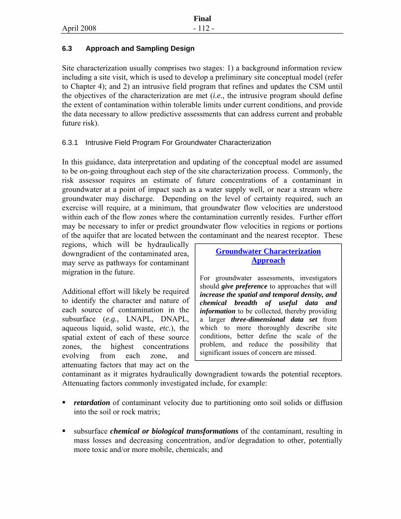
April 2008 - 112 -

Final

6.3 Approach and Sampling Design

Site characterization usually comprises two stages: 1) a background information review including a site visit, which is used to develop a preliminary site conceptual model (refer to Chapter 4); and 2) an intrusive field program that refines and updates the CSM until the objectives of the characterization are met (i.e., the intrusive program should define the extent of contamination within tolerable limits under current conditions, and provide the data necessary to allow predictive assessments that can address current and probable future risk).

6.3.1 Intrusive Field Program For Groundwater Characterization

In this guidance, data interpretation and updating of the conceptual model are assumed to be on-going throughout each step of the site characterization process. Commonly, the risk assessor requires an estimate of future concentrations of a contaminant in groundwater at a point of impact such as a water supply well, or near a stream where groundwater may discharge. Depending on the level of certainty required, such an exercise will require, at a minimum, that groundwater flow velocities are understood within each of the flow zones where the contamination currently resides. Further effort may be necessary to infer or predict groundwater flow velocities in regions or portions of the aquifer that are located between the contaminant and the nearest receptor. These regions, which will be hydraulically downgradient of the contaminated area, may serve as pathways for contaminant migration in the future.

Additional effort will likely be required to identify the character and nature of each source of contamination in the subsurface (e.g., LNAPL, DNAPL, aqueous liquid, solid waste, etc.), the spatial extent of each of these source zones, the highest concentrations evolving from each zone, and attenuating factors that may act on the contaminant as it migrates hydraulically downgradient towards the potential receptors. Attenuating factors commonly investigated include, for example:

retardation of contaminant velocity due to partitioning onto soil solids or diffusion into the soil or rock matrix;

subsurface chemical or biological transformations of the contaminant, resulting in mass losses and decreasing concentration, and/or degradation to other, potentially more toxic and/or more mobile, chemicals; and

Groundwater Characterization Approach

For groundwater assessments, investigators should give preference to approaches that will increase the spatial and temporal density, and chemical breadth of useful data and information to be collected, thereby providing a larger three-dimensional data set from which to more thoroughly describe site conditions, better define the scale of the problem, and reduce the possibility that significant issues of concern are missed.

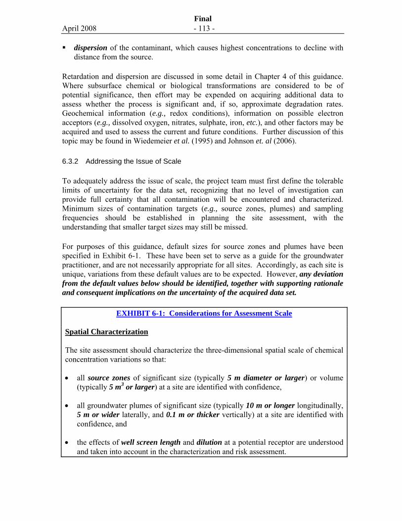
April 2008 - 113 -

Final

dispersion of the contaminant, which causes highest concentrations to decline with distance from the source.

Retardation and dispersion are discussed in some detail in Chapter 4 of this guidance. Where subsurface chemical or biological transformations are considered to be of potential significance, then effort may be expended on acquiring additional data to assess whether the process is significant and, if so, approximate degradation rates. Geochemical information (e.g., redox conditions), information on possible electron acceptors (e.g., dissolved oxygen, nitrates, sulphate, iron, etc.), and other factors may be acquired and used to assess the current and future conditions. Further discussion of this topic may be found in Wiedemeier et al. (1995) and Johnson et. al (2006).

6.3.2 Addressing the Issue of Scale

To adequately address the issue of scale, the project team must first define the tolerable limits of uncertainty for the data set, recognizing that no level of investigation can provide full certainty that all contamination will be encountered and characterized. Minimum sizes of contamination targets (e.g., source zones, plumes) and sampling frequencies should be established in planning the site assessment, with the understanding that smaller target sizes may still be missed.

For purposes of this guidance, default sizes for source zones and plumes have been specified in Exhibit 6-1. These have been set to serve as a guide for the groundwater practitioner, and are not necessarily appropriate for all sites. Accordingly, as each site is unique, variations from these default values are to be expected. However, any deviation from the default values below should be identified, together with supporting rationale and consequent implications on the uncertainty of the acquired data set.

EXHIBIT 6-1: Considerations for Assessment Scale

Spatial Characterization

The site assessment should characterize the three-dimensional spatial scale of chemical concentration variations so that:

• all source zones of significant size (typically 5 m diameter or larger) or volume (typically 5 m3 or larger) at a site are identified with confidence,

• all groundwater plumes of significant size (typically 10 m or longer longitudinally, 5 m or wider laterally, and 0.1 m or thicker vertically) at a site are identified with confidence, and

• the effects of well screen length and dilution at a potential receptor are understood and taken into account in the characterization and risk assessment.

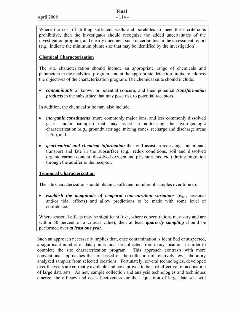
April 2008 - 114 -

Final

Where the cost of drilling sufficient wells and boreholes to meet these criteria is prohibitive, then the investigator should recognize the added uncertainties of the investigation program, and clearly document such uncertainties in the assessment report (e.g., indicate the minimum plume size that may be identified by the investigation).

Chemical Characterization

The site characterization should include an appropriate range of chemicals and parameters in the analytical program, and at the appropriate detection limits, to address the objectives of the characterization program. The chemical suite should include:

• contaminants of known or potential concern, and their potential transformation products in the subsurface that may pose risk to potential receptors.

In addition, the chemical suite may also include:

• inorganic constituents (more commonly major ions, and less commonly dissolved gases and/or isotopes) that may assist in addressing the hydrogeologic characterization (e.g., groundwater age, mixing zones, recharge and discharge areas , etc.), and

• geochemical and chemical information that will assist in assessing contaminant transport and fate in the subsurface (e.g., redox conditions, soil and dissolved organic carbon content, dissolved oxygen and pH, nutrients, etc.) during migration through the aquifer to the receptor.

Temporal Characterization

The site characterization should obtain a sufficient number of samples over time to:

• establish the magnitude of temporal concentration variations (e.g., seasonal and/or tidal effects) and allow predictions to be made with some level of confidence.

Where seasonal effects may be significant (e.g., where concentrations may vary and are within 50 percent of a critical value), then at least quarterly sampling should be performed over at least one year.

Such an approach necessarily implies that, once contamination is identified or suspected, a significant number of data points must be collected from many locations in order to complete the site characterization program. This approach contrasts with more conventional approaches that are based on the collection of relatively few, laboratory analyzed samples from selected locations. Fortunately, several technologies, developed over the years are currently available and have proven to be cost-effective for acquisition of large data sets. As new sample collection and analysis technologies and techniques emerge, the efficacy and cost-effectiveness for the acquisition of large data sets will

April 2008 - 115 -

Final

continue to improve, thereby reducing uncertainty in site characterization. For example, targeting the presence and extent of source zones at the scale of a few metres or less can be facilitated using soil vapour and/or geophysical surveys as screening approaches, with follow-up verification drilling and sampling. For vertical delineation of contamination, several direct-push technologies are now widely available that can provide continuous or near-continuous vertical profiles of soil chemistry or groundwater quality, resulting in spatial resolution at scales of a few centimetres or less. A summary of some of the more common of these technologies and their attributes and constraints is provided in Table 6.1.

6.3.3 Acquiring Groundwater Quality Information

Field investigations focused on groundwater quality will have several components, depending on investigation objectives and data needs. Virtually all will include the acquisition and chemical analysis of representative groundwater samples, which are most frequently obtained from conventional monitoring wells installed in drilled boreholes at a site. However, groundwater quality data may also be acquired using many other methods, depending on site objectives.

For risk assessment purposes, high-quality samples yielding reliable, precise and accurate chemistry data are often required, or perceived as a requirement, in the site characterization. However, if the pursuit of quality is undertaken at the expense of resolving the spatial, temporal or chemical scales that define the presence, magnitude and nature of the contamination that may be present, then the effort may be inadequate and even futile, particularly if source zones or plumes are missed.

To satisfy issues of scale, “low” quality data, sometimes referred to as “screening-level” data, can often be used successfully and economically to acquire simple measures of potential contamination over a broad area and/or vertical thickness of soil. Further screening measures may then be used specifically to acquire a relatively large number of data points, providing information on the spatial scale of the contamination. Once the scale of the problem is understood, then high-quality data may be acquired from a few strategic locations for verification and quantification. When employed effectively, this approach can provide a much more detailed understanding of the nature and extent of contamination sources and associated groundwater plumes than sampling programs based only on acquiring high-quality data from a relatively few number of conventional monitoring wells.

6.3.4 Available Technologies

Several technologies are available for groundwater characterization. Types of groundwater quality information are compared and contrasted in Table 6.1 in terms of the quality of the data provided, and the relative resolution of scale that may be achieved by the data. Spatial scales are often best satisfied by technologies that acquire many data points from many locations on a one-time basis (i.e., they provide a “snap-shot” of

April 2008 - 116 -

Final

current conditions). Of these technologies, some are more suited to resolving lateral spatial scales (e.g., mini-piezometers) while others can better resolve vertical scales (e.g., Waterloo Profiler™). Satisfying temporal scales is usually best accomplished by multiple samplings over time from permanent or semi-permanent installations (e.g., conventional monitoring wells). A summary of technogies available for locating and characterizing DNAPL contaminated sites is available in USEPA, 2004.

As noted in Table 6.1, in addition to direct methods for groundwater sampling, there are a number of indirect methods available to infer subsurface conditions and groundwater quality, and thereby supplement and/or complement a limited water quality data set. These range, for example, from qualitative, detailed descriptions and logging of field observations during drilling and sampling (e.g., odours, NAPL sheens, colour and staining, etc.), to the more complex methods of vertical profiling using special down-hole tools.

Of the indirect methods, soil profiling (i.e., profiling the soil chemistry along soil cores retrieved from a borehole) is one of several that can provide useful information on the vertical groundwater profile. Analysis of several discrete soil samples along a vertical soil column (common sampling frequencies are one sample analysed for every 0.3 m to 0.6 m of core) can often resolve the vertical distribution of contamination, and thereby address the issue of vertical scale. This, in turn, can provide the technical rationale to avoid the need to install an excessive number of wells during the characterization program. Because soil samples that are obtained from depths below the water table will contain porewater, they also provide an opportunity to roughly estimate groundwater concentrations once soil-water partitioning is taken into account. As described by USEPA (1992) and Feenstra et al. (1991), in addition to the measured soil concentration, the calculation requires an estimate of the soil organic carbon fraction (foc), as well as the soil-water partitioning coefficient (Kd).

Several indirect methods are also available that make use of certain properties of chemicals in soil or water (e.g., ultraviolet fluorescence of aromatic hydrocarbons), and can provide semi-quantitative, screening-level data with which to target a limited number of groundwater sampling locations.

With each of these indirect methods, the information obtained should be used together with other stratigraphic, hydrogeologic and chemical information, to update the CSM within the context of groundwater contaminant flow and transport.

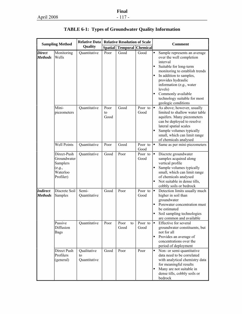
April 2008 - 117 -

Final

TABLE 6-1: Types of Groundwater Quality Information

Relative Resolution of ScaleSampling Method Relative Data Quality Spatial Temporal Chemical

Comment

Monitoring Wells

Quantitative Poor Good Good Sample represents an average over the well completion interval

Suitable for long-term monitoring to establish trends

In addition to samples, provides hydraulic information (e.g., water levels)

Commonly available technology suitable for most geologic conditions

Mini-piezometers

Quantitative Poor to Good

Good Poor to Good

As above; however, usually limited to shallow water table aquifers. Many piezometers can be deployed to resolve lateral spatial scales

Sample volumes typically small, which can limit range of chemicals analysed

Well Points Quantitative Poor Good Poor to Good

Same as per mini-piezometers

Direct Methods

Direct-Push Groundwater Samplers (e.g., Waterloo Profiler)

Quantitative Good Poor Poor to Good

Discrete groundwater samples acquired along vertical profile

Sample volumes typically small, which can limit range of chemicals analysed

Not suitable in dense tills, cobbly soils or bedrock

Discrete Soil Samples

Semi- Quantitative

Good Poor Poor to Good

Detection limits usually much higher in soil than groundwater

Porewater concentration must be estimated

Soil sampling technologies are common and available

Passive Diffusion Bags

Quantitative Poor Poor to Good

Poor to Good

Effective for several groundwater constituents, but not for all

Provides an average of concentrations over the period of deployment

Indirect Methods

Direct Push Profilers (general)

Qualitative to Quantitative

Good Poor Poor Non- or semi-quantitative data need to be correlated with analytical chemistry data for meaningful results

Many are not suitable in dense tills, cobbly soils or bedrock

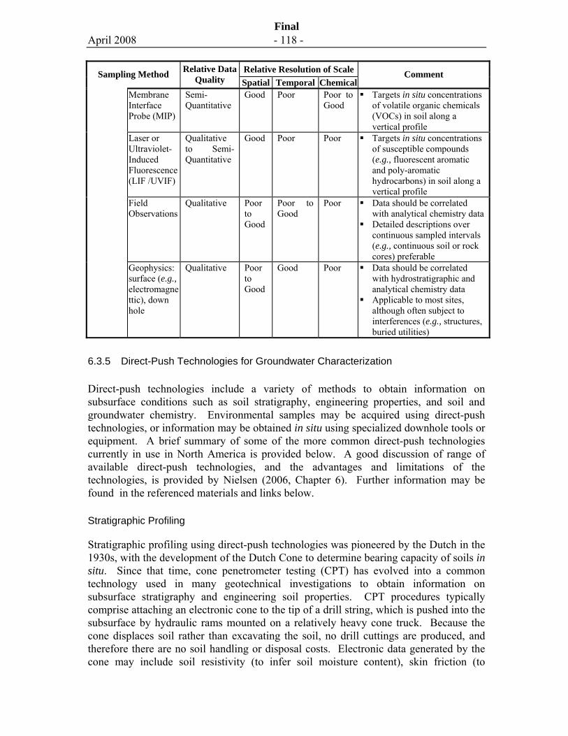
April 2008 - 118 -

Final

Relative Resolution of ScaleSampling Method Relative Data Quality Spatial Temporal Chemical

Comment

Membrane Interface Probe (MIP)

Semi- Quantitative

Good Poor Poor to Good

Targets in situ concentrations of volatile organic chemicals (VOCs) in soil along a vertical profile

Laser or Ultraviolet-Induced Fluorescence (LIF /UVIF)

Qualitative to Semi- Quantitative

Good Poor Poor Targets in situ concentrations of susceptible compounds (e.g., fluorescent aromatic and poly-aromatic hydrocarbons) in soil along a vertical profile

Field Observations

Qualitative Poor to Good

Poor to Good

Poor Data should be correlated with analytical chemistry data

Detailed descriptions over continuous sampled intervals (e.g., continuous soil or rock cores) preferable

Geophysics: surface (e.g., electromagnettic), down hole

Qualitative Poor to Good

Good Poor Data should be correlated with hydrostratigraphic and analytical chemistry data

Applicable to most sites, although often subject to interferences (e.g., structures, buried utilities)

6.3.5 Direct-Push Technologies for Groundwater Characterization

Direct-push technologies include a variety of methods to obtain information on subsurface conditions such as soil stratigraphy, engineering properties, and soil and groundwater chemistry. Environmental samples may be acquired using direct-push technologies, or information may be obtained in situ using specialized downhole tools or equipment. A brief summary of some of the more common direct-push technologies currently in use in North America is provided below. A good discussion of range of available direct-push technologies, and the advantages and limitations of the technologies, is provided by Nielsen (2006, Chapter 6). Further information may be found in the referenced materials and links below.

Stratigraphic Profiling

Stratigraphic profiling using direct-push technologies was pioneered by the Dutch in the 1930s, with the development of the Dutch Cone to determine bearing capacity of soils in situ. Since that time, cone penetrometer testing (CPT) has evolved into a common technology used in many geotechnical investigations to obtain information on subsurface stratigraphy and engineering soil properties. CPT procedures typically comprise attaching an electronic cone to the tip of a drill string, which is pushed into the subsurface by hydraulic rams mounted on a relatively heavy cone truck. Because the cone displaces soil rather than excavating the soil, no drill cuttings are produced, and therefore there are no soil handling or disposal costs. Electronic data generated by the cone may include soil resistivity (to infer soil moisture content), skin friction (to

April 2008 - 119 -

Final

measure soil cohesive strength), and piezometric head (i.e., hydraulic head). The data are typically acquired at a resolution of a few centimetres or less, yielding a very detailed vertical profile of soil properties and inferred stratigraphy. Depths of 30 m or more may be profiled under favourable soil conditions.

Over the past decade, specialized sampling tools and procedures have been developed to obtain multiple groundwater samples along a vertical profile, and in situ measurements of soil chemical conditions. Common direct-push technologies include the Waterloo Profiler™, laser-induced fluorescence (LIF), membrane interface probes (MIP), and others (e.g., www.clu-in.org/download/remed/542r05007.pdf). A few of these are further discussed below.

Groundwater Profiling

Groundwater profiling gained prominence in the late 1980s and early 1990s with the development of the Waterloo Profiler™ (Pitkin et al., 1999). The Waterloo Profiler™ comprises a steel tip with small-diameter screened ports connected to small-diameter tubing (typically quarter-inch). The tip is fitted to a hollow drill string (e.g., “A” rods), with the tubing running up the hollow centre of the rods to ground surface, where a groundwater sample may be acquired into a vial using a peristaltic pump. During tip advancement, water may be pumped at very low flow rates downhole and into the probe to assist in keeping the screened ports open and silt-free. During a typical application, groundwater samples are obtained at depth intervals of 0.3 m to 0.5 m, providing relatively good resolution of the groundwater profile. The technology can be very useful where the water table is relatively shallow (the use of a peristaltic pump limits the effective depth of the water table to a few metres or less below ground surface), and where small sample sizes are adequate for chemical analysis (e.g., 40 mL samples, although larger sample sizes can be obtained). Caution is advised at highly contaminated sites, where there is some possibility of contaminant dragdown, leading to an overestimate of the thickness of the contaminated zone.

Other technologies are available that can be used to develop groundwater profiles including the Hydropunch sampler (www.state.nj.us/dep/srp/regs/agws/agws_06.htm) which can be deployed using a hollow-stem auger drill rig, and the Geoprobe sampler, which can be deployed from direct-push rigs (www.geoprobe.com).

April 2008 - 120 -

Final

Laser-Induced Fluorescence

Laser-induced fluorescence (LIF), sometimes referred to as ultraviolet-induced fluorescence (UVIF), is a technology based on variable or fixed wavelength lasers (typically an ultraviolet wavelength). The laser transmits optic pulses into an optic fibre, which runs down a CPT drill string to a 6.4 mm diameter sapphire window that is mounted flush with the probe rod, approximately 0.6 m above a standard CPT cone. The ultraviolet light excites molecules of aromatic hydrocarbons that may be present in soil at the window, and causes them to fluoresce. Emitted light is carried back to a detector at ground surface via a second optic fibre. The spectral intensity of the fluorescence can be directly related to the concentration of the aromatic hydrocarbons present, allowing concentrations to be quantified. In field applications, LIF results are often calibrated in the field by comparison against soil concentrations in samples obtained from an adjacent borehole. Contaminants that can be measured using LIF technology include petroleum hydrocarbons (e.g., gasoline, diesel, kerosene) , coal tars, creosote, and any other liquid containing significant concentrations of aromatic hydrocarbons (e.g., www.clu-in.org/char/technologies/lif.cfm).

Membrane Interface Probe

The membrane interface probe (MIP) comprises a semi-permeable membrane mounted flush with the side of a cone. After pushing the cone to the desired depth, the membrane is heated to between about 100oC and 125oC, promoting diffusion of VOCs in the soil across the membrane into the probe, where a carrier gas sweeps the inside of the membrane and carries the gas to surface. Detectors at surface record VOC concentrations in the gas, as well as soil electrical conductivity and temperature. VOC concentrations may be measured semi-quantitatively using various detectors such as photo-ionization detectors (PID), flame ionization detectors (FID) and electron capture detectors (ECD). Quantitative measurements may be made by coupling the system with a GC mass spectrometer.

The MIP has become a relatively common direct-push technology for the in situ quantification of volatile organic compound (VOC) concentrations in soil, and to infer the presence of LNAPL and DNAPL. Measurements are commonly made over short depth intervals (about 0.3 m intervals), providing a vertical profile or log of concentrations with depth. Examples of purveyors of the technology may be found from the following links: www.geoprobe.com/diweb/products/mip/mip.htm, www.teamzebra.com/mip.htm,www.precisionsampling.com/membrane_interface_probe.html, www.vironex.com/pages/equip_mip.html.

Other Technologies

A range of tools have been or are currently under development to provide quantitative in situ measurements of specific compounds or groups of compounds. Some examples are discussed by Nielsen (2006, Chapter 6), and are provided below:

April 2008 - 121 -

Final

• fuel fluorescent detectors for sensing petroleum hydrocarbons;

• CPT-based Raman spectroscopy to detect a variety or compounds including, metals and metals complexes, DNAPLs (e.g., TCE and PCE);

• metals sensors using x-ray diffraction (XRF) or laser-induced breakdown spectroscopy; and,

• explosives sensors to characterize soil containing various nitro-aromatic explosives materials.

6.4 Acquiring Hydrogeologic Information

In addition to satisfying issues of scale related to the presence, distribution and fate of the contaminants, it is imperative that the groundwater characterization program define site-specific hydrogeologic conditions (e.g., the presence, extent and properties of underlying aquifers and aquitards, groundwater flow direction and velocities, etc.). These should be resolved at a scale that is compatible with the size of the contamination sources and associated plumes, and the rate of plume migration and evolution. Stratigraphic conditions should be well-defined over the area where the contamination sources and plumes currently exist, and over the predicted region that they may occupy in the future. Stratigraphic conditions should also be understood in detail within the vertical zone or thickness of soil that is contaminated, with particular emphasis on defining or estimating permeability and permeability contrasts among the various strata and the potential for preferential pathways for contaminants.

Hydrogeologic information is commonly acquired through drilling, well installation, and well monitoring and testing programs. Soil and/or rock core samples are usually obtained and used to describe physical aquifer conditions, and hydraulic tests or measurements are made to acquire hydraulic information about the aquifer. Field tests may range from simple static water-level measurements that can be used to assess the water table or piezometric surface of the aquifer, to more involved aquifer pumping tests that hydraulically stress a region of the aquifer, and thereby allow estimation of local and/or regional-scale hydraulic parameters (e.g., hydraulic conductivity, storativity, etc.). Further information on this topic can be found in various reference texts (e.g., Fetter, 2001; Domenico and Schwartz, 1998; Freeze and Cherry, 1979).

6.4.1 Groundwater Flow Direction

Almost all characterization programs that address groundwater contamination need to clearly identify groundwater flow direction and velocity in each of the flow zones of interest. Commonly, flow direction is established by obtaining groundwater elevations from monitoring wells at several locations within the same aquifer, and posting and contouring the data. Where the wells are completed with long well screens (e.g., a metre or more in length), and/or at different depths within the aquifer, problems may arise

April 2008 - 122 -

Final

where vertical hydraulic gradients are also present within the aquifer, or when data are used from wells that are installed across more than one aquifer or groundwater flow zone. Because the measured water level in a well actually represents a quasi-average of hydraulic heads encountered across the well completion interval, the resulting contour map may suggest unusual, inexplicable and erroneous patterns of hydraulic head and groundwater flow. Poor well construction methods may also allow flow between zones, and serve as conduits allowing contaminant migration between the zones.

In addition to the potential problems with long well screens, the presence of LNAPL in a well may also yield erroneous measurements of water elevation. Where significant floating LNAPL is present, the elevation of the LNAPL must be corrected to determine the actual groundwater elevation, to account for the density difference between the LNAPL and groundwater. As discussed by SABCS (2006), the water elevation can be calculated using the relative density of the oil to water (ρro), the elevation of the water-oil interface (Zow, m), and the LNAPL thickness measured in the well (Ho, m). The theoretical water elevation (Zaw, m) in a well containing LNAPL can be estimated as follows:

Zaw = Zow + (ρroHo) [6-1]

It also should be recognized that the thickness of NAPL measured in a monitoring well is commonly greater than the actual NAPL-saturated thickness of the formation. Further discussion of this topic is provided by API (2003).

Identifying and/or avoiding such pitfalls can be facilitated as the field data are acquired by preparing simple two-dimensional stratigraphic cross sections, or two- or three-dimensional visualizations of the field stratigraphic and hydrogeologic information. By undertaking such forms of data assessment and interpretation in the field, and routinely updating the CSM, issues can be identified, and timely and effective field decisions can be made. Once an issue is identified, efforts can be directed towards avoiding cross-communication between flow zones through appropriate design (e.g., using small well screens, targeting well completions to monitor specific depths and/or single flow zones within the aquifer, using alternative characterization approaches, etc.). Where cross-communication is known or suspected to have occurred, consideration should be given to promptly removing the well installation so that present or future cross contamination is avoided.

6.4.2 Groundwater Velocity

Groundwater velocity estimates are commonly derived using a simple analytical model, which is a modification of the Darcy equation:

v = K * i / n [6-2]

April 2008 - 123 -

Final

where v is the estimated advective groundwater velocity, K is the formation hydraulic conductivity, i is the hydraulic gradient, and n is the effective porosity of the aquifer. Of these variables, n typically falls within the range of 0.2 to 0.5 (Freeze and Cherry, 1979) and is rarely measured. The hydraulic gradient, i, is commonly calculated based on simple field measurements of static groundwater levels in monitoring wells. Provided that the flow direction is estimated appropriately, then the contoured data may be used as a reliable estimate of i. The hydraulic conductivity, K, may be estimated by a variety of means, depending on the level of certainty required. Common methods include:

• use of simple “textbook” values, based on descriptions of soil type, with no actual field tests conducted (simplest approach with highest uncertainty);

• use of empirical relationships drawn between soil grain size and hydraulic conductivity (e.g., Hazen method, as described by Freeze and Cherry, 1979, and Fetter, 2001) (unreliable for soil with more than a few percent of fine materials);

• single-well response tests, also referred to as slug tests, which are field tests performed at individual monitoring wells, and provide an indication of local horizontal hydraulic conductivity at the well screen;

• laboratory permeameter tests, conducted on small samples (typically a few centimetres in length) of formation material (many tests may be required to estimate large-scale hydraulic conductivity);

• pumping tests, conducted on individual wells, with water-level drawdowns monitored at other wells (this approach stresses a much larger volume of aquifer than single-well response tests, and commonly provides more useful and reliable information);

• tidal response analyses, whereby changes in water levels caused by tidal action are monitored and used to estimate formation hydraulic conductivity (as with pumping tests, tidal response analyses provide relatively reliable, large-scale estimates of hydraulic conductivity); and,

• tracer tests, whereby the travel time of a groundwater tracer (usually a large inorganic anion such as chloride), is monitored over time and used to directly estimate velocity (usually the most accurate method to estimate velocity).

Each of the variables used to estimate groundwater velocity should be defined with a level of certainty (e.g., plus or minus twenty percent, one hundred percent, order of magnitude, etc.) so that the uncertainty in the velocity estimate, which is usually expressed as a range, can be provided and is sufficiently narrow for decision-making purposes. In calculating groundwater velocities, i and n carry relatively little uncertainty when compared with estimates of K, which commonly vary by factors of two to ten or more within an aquifer, both vertically and laterally. As noted above, the more

April 2008 - 124 -

Final

sophisticated (and usually more costly) methods for estimating K usually provide a higher level of certainty than the simple approaches.

For many site assessments, tightly bounded estimates of groundwater velocity are not necessary, and the investigator may use relatively low-cost approaches to derive an estimate. For example, crude approximations may be appropriate where the distance to the nearest groundwater receptor is several kilometres, and soil conditions are known to be fine-grained and therefore poorly conductive. In such cases, gross estimates of hydraulic conductivity (e.g., textbook values for different soil classes) and measured hydraulic gradients may be all that is necessary to adequately address velocity.

Where greater certainty is desired, such as may occur when the travel time to a receptor is of critical importance, then more sophisticated methods with tighter bounds of uncertainty should be used.

Where the receptor is located some distance hydraulically downgradient of the site, this will also require an assessment of the hydraulic properties of the aquifer (e.g., K and n) through which the contaminants must travel, and the hydraulic gradient. Where the properties are not known or cannot be estimated with reasonable certainty, then in-situ investigation will likely be required.

6.5 Monitoring and Monitoring Networks

While groundwater monitoring is often undertaken to provide a snapshot of current conditions within an aquifer, a network of monitoring points or wells may be established at a site to serve as “sentinel” wells to monitor the progress or confirm the absence of particular contaminants at a location, or to establish temporal trends in plume behaviour. The design of the monitoring wells and the monitoring well network requires careful consideration of the local hydrostratigraphic conditions, and the receptor who may receive and potentially become exposed to the affected groundwater.

6.5.1 Well Screen Length and Well Completion Intervals

Groundwater supply wells in both porous and rock media are commonly designed to extract acceptable quality water at a high sustainable flow rate. Such wells typically have well screens in excess of one metre in length, and may have multiple screened intervals along the well bore, sometimes intercepting multiple aquifer zones. While the wells are designed for maximizing productivity, they may not always intercept all productive zones within a particular aquifer system. Because the groundwater quality from such wells represents an average condition, it is important from a characterization perspective that site characterization data are acquired at a smaller scale than the supply wells, so that any averaging effect is understood. Vertical variations and trends in the spatial distribution of site contamination should be assessed and taken into account in the characterization program.

April 2008 - 125 -

Final

Effectively, this means that the maximum monitoring interval in wells for site characterization purposes should be, at most, the shortest expected screen length of a water supply well and, preferably, much shorter than the screen length of a water supply well. Further, at least one of the wells in the monitoring network should be placed within the depth interval, and at the most likely location, where highest concentrations occur in the aquifer so that the relevance of any averaging of chemical conditions in the aquifer can be better understood and addressed from a risk perspective.

In absence of a site-specific rationale that establishes the maximum well screen lengths for a monitoring network, the following guidance is provided in Exhibit 6-2:

As part of the rationale used to select screen length for monitoring wells in a site characterization program, the monitored interval should be sufficiently small to resolve the contamination at a vertical scale that allows reasonable predictions of concentrations to be made at a receptor. For example, where the receptors may be water supply wells of uncertain design, then expected variations in design of the water supply wells, and their variable positions in the aquifer, should be taken into account when predicting future concentrations at the receptors. For purposes of this guidance, the monitoring interval should be, at most, 1.5 m in length. Thus, for example, where supply wells that are potential receptors may have long screens (e.g., several metres in length), site characterization using monitored intervals of 1.5 m or less would be expected to provide data at a scale that would allow reasonable predictions to be made at such receptors. As each site is unique, variations from these default values are to be expected. However, any deviation from the default values should be identified, together with supporting rationale and consequent implications on the uncertainty of the acquired data set.

Advances in the development of direct-push technologies allow for detailed vertical profiling of groundwater chemistry so that acquisition of data over intervals of 0.3 m or less can often be readily achieved. Alternatively, analysis of discrete soil samples using either in situ (e.g., MIP or LIF) or ex situ sampling approaches at closely spaced intervals (e.g., 0.3 m or less) can also be used to effectively establish vertical profiles of relative concentrations in groundwater. Such information may be used together with groundwater chemistry data from conventional monitoring wells, to semi-quantitatively predict the expected groundwater quality that may be obtained from wells with shorter screen lengths, or from wells placed at other locations and/or depths within the aquifer.

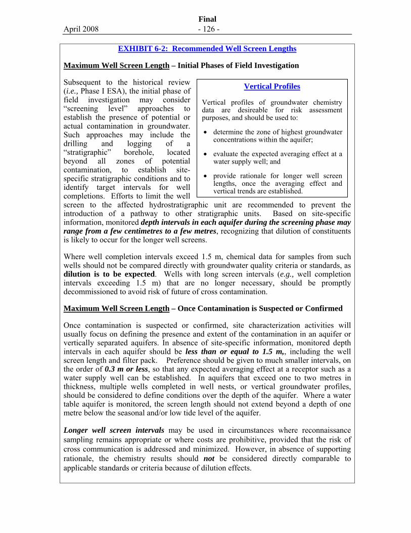
April 2008 - 126 -

Final

Vertical Profiles

Vertical profiles of groundwater chemistry data are desireable for risk assessment purposes, and should be used to:

• determine the zone of highest groundwater concentrations within the aquifer;

• evaluate the expected averaging effect at a water supply well; and

• provide rationale for longer well screen lengths, once the averaging effect and vertical trends are established.

EXHIBIT 6-2: Recommended Well Screen Lengths

Maximum Well Screen Length – Initial Phases of Field Investigation

Subsequent to the historical review (i.e., Phase I ESA), the initial phase of field investigation may consider “screening level” approaches to establish the presence of potential or actual contamination in groundwater. Such approaches may include the drilling and logging of a “stratigraphic” borehole, located beyond all zones of potential contamination, to establish site-specific stratigraphic conditions and to identify target intervals for well completions. Efforts to limit the well screen to the affected hydrostratigraphic unit are recommended to prevent the introduction of a pathway to other stratigraphic units. Based on site-specific information, monitored depth intervals in each aquifer during the screening phase may range from a few centimetres to a few metres, recognizing that dilution of constituents is likely to occur for the longer well screens.

Where well completion intervals exceed 1.5 m, chemical data for samples from such wells should not be compared directly with groundwater quality criteria or standards, as dilution is to be expected. Wells with long screen intervals (e.g., well completion intervals exceeding 1.5 m) that are no longer necessary, should be promptly decommissioned to avoid risk of future of cross contamination.

Maximum Well Screen Length – Once Contamination is Suspected or Confirmed

Once contamination is suspected or confirmed, site characterization activities will usually focus on defining the presence and extent of the contamination in an aquifer or vertically separated aquifers. In absence of site-specific information, monitored depth intervals in each aquifer should be less than or equal to 1.5 m,, including the well screen length and filter pack. Preference should be given to much smaller intervals, on the order of 0.3 m or less, so that any expected averaging effect at a receptor such as a water supply well can be established. In aquifers that exceed one to two metres in thickness, multiple wells completed in well nests, or vertical groundwater profiles, should be considered to define conditions over the depth of the aquifer. Where a water table aquifer is monitored, the screen length should not extend beyond a depth of one metre below the seasonal and/or low tide level of the aquifer.

Longer well screen intervals may be used in circumstances where reconnaissance sampling remains appropriate or where costs are prohibitive, provided that the risk of cross communication is addressed and minimized. However, in absence of supporting rationale, the chemistry results should not be considered directly comparable to applicable standards or criteria because of dilution effects.

April 2008 - 127 -

Final

6.5.2 Horizontal Spacing of Data Points

In the horizontal plane, the spacing of chemistry data points acquired using monitoring wells or other means should be sufficient to resolve the boundary of a contaminant plume at an appropriate scale. As a guide for establishing appropriate scales, it is assumed in this guidance that lateral dispersion of the plume is minimal whereas longitudinal dispersion is significant, and that longitudinal dispersion is both velocity- and scale-dependent. Under these assumptions, the appropriate scale selected to encounter potential plumes and resolve their width should be compatible with the size of contaminant source zone at each AEC. Assuming AECs of at least 5 m in diameter, then lateral well separations of about 5 m are appropriate. The appropriate scale for establishing and monitoring plume length will be highly dependent on groundwater and contaminant velocity, and the size of the plume, and should be established after reasonable estimates for these variables have been determined.

Dispersion is much more significant in the longitudinal direction, and the degree to which the longitudinal extent of contamination is resolved may be influenced by several constraints and data needs. For example, these may include the need to define the presence or absence of contamination at particular property boundaries or potential receptors, or the need to quantify contaminant transport velocities. Velocities that are estimated based on the known extent of the plume emanating from a source, and the initial time of release at the source, can often be used to estimate travel times to the nearest receptor with a relatively high degree of confidence. In such a case, better definition of the extent of the plume is likely to yield a more reliable estimate of velocity.

Figure 6-3 provides an example of a site where data were acquired at an inappropriate scale to resolve the locations and extent of source zones and associated plumes of contamination. Data contours using different interpolation assumptions and the same data set yielded remarkably different interpretations of groundwater chemistry. Much more closely spaced monitoring wells would be necessary at the site to resolve the contamination for purposes of remediation and/or risk management.

In absence of site-specific information on the size of a source zone and the groundwater velocity, the following guidance is provided in Exhibit 6-3:

EXHIBIT 6-3: Recommended Well Spacing

Minimum Horizontal Separation – Initial Phases of Investigation

In the initial phases of investigation, monitoring well locations should be selected with the intent to intercept highest concentrations of potential contaminants evolving from each potential source zone. However, because groundwater flow direction is unlikely to be established with precision during the initial phases, and the presence and extent of each source zone is probably not known, screening approaches (e.g., wells with long

April 2008 - 128 -

Final

screen intervals, location selection based on geophysics, soil vapour surveys, local topography or bedrock geology) are sometimes appropriate.

The data from screening-level assessments should almost always be viewed with caution, and usually should not be regarded as conclusive with respect to the absence of contamination. For example, subtle differences between actual and assumed groundwater flow direction, and the dilution effects of relatively long well screens, may lead to erroneous conclusions regarding the presence of low but detectable levels of contamination. To circumvent these shortcomings, groundwater flow direction should be established during the initial phases of investigation, and the data used to re-assess the optimum sampling locations with respect to anticipated highest concentrations. Further, groundwater quality data should be considered “preliminary.” Other than the absence (i.e., non-detection) of contaminants of potential concern, or the presence of contaminants at concentrations less than one-tenth of the applicable standard or criteria, further assessment of the groundwater pathway should be conducted.

Minimum Horizontal Separation – Once Contamination is Suspected or Confirmed

Once groundwater contamination is suspected or confirmed, and groundwater flow direction has been established, horizontal separations for wells or similar data points should be on the order of 20 m to 50 m in the longitudinal direction (along the expected direction of groundwater flow) and 10 m to 20 m transverse to flow. Exceptions may occur, for example, where large source zones are known to be present, or where the aquifer is relatively homogeneous and groundwater flow velocities are high. In such cases, site-specific rationale should be provided to justify the well separation distances.

Once the locations and sizes of all source zones of groundwater contamination have been identified, the lateral spacing should be adjusted accordingly. At the final selected scales, the uncertainty associated with “missing” a relatively narrow plume and its consequences on predicted groundwater quality at a supply well should be assessed, documented in the assessment report and communicated to the risk assessor.

For groundwater characterization programs aimed at defining the extent of source zones that may evolve vapours to the vadose zone, a much smaller scale of resolution, on the order of 5 m or less, is typically necessary in order to resolve the extent of the zone and evaluate risk. Site specific conditions will dictate the most appropriate scale.

Resolution of plume sizes at smaller scales will reduce uncertainty and provide more confidence in predicted concentrations. In addition, or as an alternative, to installing and sampling more monitoring wells, methods to reduce uncertainty may include, but are not limited to:

• use of direct-push technologies, such as MIP or LIF;

April 2008 - 129 -

Final

• groundwater pumping tests to evaluate and sample larger volumes of aquifer material than can be obtained using single monitoring points;

• geophysics to map certain types of plumes (e.g., highly conductive shallow groundwater plumes such as dissolved salts); and,

• soil vapour surveys to more accurately map source zones associated with VOCs such as NAPL.

6.5.3 Vertical Spacing of Data Points

Vertically, a groundwater plume should be resolved to a scale that is compatible with the scale at which the groundwater is used, such as the screen length of a groundwater supply well. However, site characterization also must consider the scale of the stratigraphic layering that is likely present, and the presence and evolution of contaminant plumes as they encounter and migrate through the various strata. In absence of site-specific rationale, data to define and bound the vertical extent and thickness of a plume should be derived from locations that are separated vertically by no more than one metre from the bottom of one well and the top of the next, within each aquifer of interest. Where monitoring wells are used, care must be taken to select a practical small monitored interval, to avoid cross-communication between aquifers, or even between significant stratigraphic layers within the same aquifer.

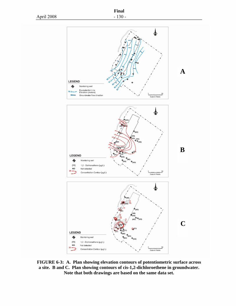
April 2008 - 130 -

Final

FIGURE 6-3: A. Plan showing elevation contours of potentiometric surface across a site. B and C. Plan showing contours of cis-1,2-dichloroethene in groundwater.

Note that both drawings are based on the same data set.

A

C

B

April 2008 - 131 -

Final

6.6 Field and Laboratory Data Acquisition

Several types of groundwater information are best acquired in the field rather than by a fixed analytical laboratory, with the proviso that the data are acquired by trained personnel using acceptable procedures and protocols. Important field measurements such as groundwater pH, temperature, dissolved oxygen, redox potential, electric conductivity, and alkalinity should only be taken in the field as they are subject to significant and often rapid changes once the groundwater has been removed from the subsurface. Such data and procedures should be provided in the site assessment report, as they are often critical to the interpretation of site conditions.

These and other measurements that are easily obtained in the field can provide the investigator with useful information to direct the field program. For example, electrical conductance is simply measured with a probe and provides a rapid estimate of total dissolved solids content, which sometimes serves as an excellent indicator of plume strength such as landfill leachate. Total organic vapour concentrations, measured in the head space of an enclosed jar sample of groundwater using an organic vapour meter, can often provide a rapid estimate of total volatile organic chemical concentrations in the water sample. In addition to simple probes, several types of direct measurements of soil or groundwater chemistry can also be obtained using direct push technologies, such LIF and MIP (see Table 6.1).

6.6.1 Well Development

Where data are to be acquired using samples from monitoring wells, it is important that the well is developed soon after installation, to remove fluids potentially introduced to the well during drilling, and to remove particulates that may have become entrained in the well and filter pack. However, well development should not be performed prior to 24 hours after installation in order to ensure proper hydration of sealant (bentonite) and proper setting of grout. Well development can be achieved in several ways. Some of the more common methods involve a) use of a surge block to flush and move water in and out of the well screen, and then to surface, and b) briefly over-pumping and then resting the well using a submersible pump, and c) air-lifting fluids from the well by injecting air from a compressor through a downhole pipe that discharges the air near the well bottom. Development should be conducted by experienced personnel to avoid compromising the integrity of the well and formation.

April 2008 - 132 -

Final

6.6.2 Well Purging and Sampling

Following well development, it is unlikely that the monitoring well will be in equilibrium with conditions in the surrounding geologic medium. For example, the sand filter pack between the well and geologic formation will not be in geochemical equilibrium, gases may have been introduced where drilling methods such as air rotary have been used, and NAPL, if present in the formation, may not have achieved a new static equilibrium with respect to well and pore geometry and hydraulic pressures following drilling. In tight clays, well development may lead to a week or longer delay as the well recharges. To reduce uncertainty in the subsequent monitoring data set, it is common practice to acquire samples at least one week following well development and preferably after two weeks. However, it is recognized that, in some circumstances, near-immediate results are required. For purposes of this guidance, the following practice is recommended.

At the time of sampling, groundwater is usually first removed from the well and field measurements are monitored over time prior to sample collection in a process referred to as purging. Once “stabilized”, the measurements are used to infer that representative groundwater conditions are present, and that a representative groundwater sample for chemical analysis can now be obtained.

The most common practice used to obtain reliable field measurements (e.g., pH, conductivity, temperature and others) involves placement of field probes into a flow-through cell. As groundwater is pumped from a monitoring well through the cell, direct measurements of each variable are then obtained from calibrated instruments attached to the probes. Stabilization of field parameters is likely to be indicative of a quasi-equilibrium condition and subsequent samples may be considered representative of the aquifer. Where a flow-through cell is not used, care must be taken to minimize exposure of the water to the atmosphere prior to measurement. Even a few seconds exposure to the atmosphere may significantly alter readings of variables such as dissolved oxygen.

Conventional purging practice is to remove at least three to five “well volumes” prior to sampling, where a well volume comprises the volume of standing water in the well. Some practitioners include the additional water volume entrained in the sand filter pack in the annulus between the wells screen and borehole wall. Either approach is usually acceptable, provided that the practice is consistent among wells and different sampling events. Methods used and volumes purged should be reported as part of the site assessment report.

Resting Time Between Well Development and Sampling

Groundwater sampling from newly installed monitoring wells should be conducted at least one week following well installation and development. Where shorter intervals are desired or required, the data acquired should be considered “preliminary” until a subsequent second sample can be obtained and analysed after one week to confirm or revise the data set. To provide further certainty, particularly where decisions are to be made based on the absence of contamination, at least two samples should be obtained on different dates, separated by at least one month, for analysis of the constituents of concern.

April 2008 - 133 -

Final

In many site investigations, project objectives often necessitate installation of monitoring wells in relatively low-permeability formations (e.g., clays and silts, or fractured rock). Purging such wells is sometimes difficult, and frequently results in purging the well dry. In such situations, it is recommended that such wells be carefully and slowly purged, with the objective of avoiding dewatering of the well screen (Puls and Barcelona, 1996). The purge water should be monitored for field parameters. Water levels in the well should be recorded at the beginning and end of the purging process, and then be allowed to recover prior to sampling. Where water-level recovery may take several hours to days, it must be recognized that the sampled water is likely to have established partial or full equilibrium with atmospheric conditions, and that a truly representative groundwater sample may not be possible. In particular, volatile organic chemicals may be substantially lower in the sample than the groundwater, and constituents such as metals may be biased low due to precipitation.

Within the context of well averaging that occurs while pumping, as discussed previously, it should be recognized that the stable field measurements (conductivity, temperature, turbidity, and pH) are likely to be indicative of a quasi-equilibrium condition. The groundwater sample obtained following purging will represent a mixture of formation waters that enter the well screen from the various permeable zones encountered at the well screen and/or well filter pack. Uniform purging and sampling techniques serve to stabilize the mixing process, yielding stabilized field measurements.

Once conditions in the well are considered stable, then a variety of acceptable sampling methods are available to acquire the groundwater sample. Several methods are briefly discussed below:

• Conventional Sampling Approaches - Some of the more common sampling methods used to recover groundwater samples include the use of bailers, inertial lift pumps (e.g., Waterra™), bladder pumps and downhole submersible electrical pumps. When applied conventionally, the pumps are used to purge the well of at least three to five volumes of water from the well prior to sample collection. Field parameters, as discussed above, are monitored to infer that representative groundwater conditions have been achieved. In low-permeability formations, it may not be possible to remove at least three well volumes of water from the well, thus fewer well volumes, or alternative sampling methods, should be considered, recognizing that the sample may not truly represent groundwater conditions. Once purging is complete, samples are then obtained in sample containers and preserved, if required, prior to transport (usually in a chilled container) to the analytical laboratory for analysis.

• Low-Flow Purging and Sampling – Low-flow purging and sampling refers to procedures that minimize the flow of water through a well screen during pumping, resulting in less disturbance at the well screen and production of a smaller volume of purge water prior to obtaining a stable, representative groundwater sample. Common techniques involve setting the tubing or intake of a pump (e.g., peristaltic, bladder, centrifugal, variable speed low-flow electrical submersible) at the well

April 2008 - 134 -

Final

screen and withdrawing formation water at rates of about 100 to 500 mL/minute (Puls and Barcelona, 1996). Withdrawal rates in excess of one litre per minute should be avoided. Water levels are typically monitored during purging, to ensure that minimal formation drawdowns (i.e., about ten centimetres or less is preferred but not mandatory) are achieved. With low-flow sampling, the intake of the sampling device is set at a low velocity to minimize drawdown in the well, thereby minimizing hydraulic stress and disturbance on the well and adjacent geologic formation. Greater stable drawdowns (i.e., greater than ten centimetres) may yield acceptable samples, although the increased hydraulic stress imposed on the formation at the well screen may yield disturbed (e.g., turbid) samples. In situations where the well is completed in a low-permeability formation, it may be necessary to purge at very low flow rates (i.e., less than 100 mL/minute), taking care to avoid dewatering the well screen (Puls and Barcelona, 1996). If dewatering remains a problem, then alternative approaches, such as no-flow or passive sampling described below, should be considered. Where applicable, low-flow sampling of monitoring wells is usually favoured over conventional procedures (e.g., bailers or inertial lift pumps) because minimized disturbance at the well screen during sampling will also minimize volatilization losses and re-suspension of colloidal materials. The procedure also usually reduces the volume and handling of large volumes of purge water. A suggested low-flow sampling procedure is provided in SOP #3.

• No-flow Purging and Sampling - No-flow purging and sampling refers to sampling procedures that negate the need for any purging prior to sample collection. Examples include micro-purging, where in only the sample tubing of, for example, a peristaltic pump is purged prior to sample collection, and discrete downhole samples (e.g., Hydrasleeve™, www.dsienv.com/Hydrosleeve.htm; and Snap Sampler™, www.snapsampler.com), wherein a sampling device is submersed downhole, opened and filled at a discrete depth, and returned to surface for chemical analysis. Sampling using such approaches is predicated on the assumption that the natural horizontal groundwater flux across a monitoring well screen is sufficiently high to develop groundwater chemical conditions in the well that are representative of conditions in the adjacent geologic formation. Such an assumption is likely to be valid in permeable formations (e.g., sands and gravels), but may be invalid in less permeable materials where stagnant water may be present in the well. Where the approach is used, it should be validated for site-specific conditions by comparison with alternative conventional or low-flow procedures. Alternatively, the techniques should be considered to provide screening level information to determine the presence or absence of potential contamination.

• Passive Diffusion Sampling – Passive diffusion sampling refers to a group of sampling devices that are typically composed of elongate semi-permeable membrane bags (often polyethylene plastic), which can be submersed in monitoring wells, allowed to equilibrate, and then withdrawn for chemical analysis. The bag is filled with a liquid (usually distilled water) and inserted to a discrete depth within the well screen of a monitoring well. After allowing a period to achieve chemical equilibrium across the membrane (usually several days), the bag is retrieved and the

April 2008 - 135 -

Final

liquid analysed for the constituents of concern. Single and multi-interval passive diffusion bags are available. Similar to no-purge sampling, passive diffusion bags rely on the assumption that the groundwater in the monitoring well is not stagnant, but rather, represents conditions in the aquifer adjacent to the well screen. Consequently, similar caveats on their use should be applied as those for no-flow sampling. A comparison of discrete sampling devices and passive diffusion bags is provided at the following link: http://el.erdc.usace.army.mil/elpubs/pdf/trel05-14.pdf.

It is recommended that dates for drilling, well development, and sampling be noted in field notes.

6.6.3 Field Laboratories

With respect to quantitative groundwater chemistry data, data acquisition in the field by a field laboratory can sometimes be beneficial to the program as it can allow timely decisions to be made as the investigation program proceeds. Changes in chemistry resulting from factors such as mass losses are usually minimized because the groundwater samples are preserved, sealed and refrigerated soon after retrieval. The advantages of a field laboratory are often of more significance for analysis of soil rather than groundwater, because soil samples are much more prone to chemical losses resulting from volatilization and degradation.

6.6.4 Special Considerations

Metals

Where groundwater samples are obtained for quantifying metals concentrations, it is important that the samples be filtered in the field during or immediately after retrieval, and prior to preserving the sample (e.g., with nitric acid). Typically a clean 0.45 micron membrane filter is employed. Because aquifers normally act as filters and prevent significant migration of particulates, analysis of samples containing particulates will not represent actual groundwater conditions. Unfiltered samples, when analysed by a laboratory, will commonly contain elevated metals concentrations because the particulates contain metals and are digested at the laboratory prior to analysis. On the other hand, filtered samples may contain non-representative low metals concentrations if the sample was allowed to sit for some time prior to filtering, allowing dissolved metals to precipitate from the water as a consequence of gas exchange and a rise in redox potential.

NAPLs

Caution should be exercised when drilling, installing and sampling wells suspected to contain NAPL. Many NAPLs are clear and colourless, or are easily missed because they co-dissolve natural organic materials, taking on the same colour as the surrounding

April 2008 - 136 -

Final

medium. If suspected, meticulous care should be taken to avoid cross contamination and drawdown from one water-bearing unit to another. Once the well is installed, monitoring should be conducted to determine NAPL presence. Special probes, such as an interface meter (e.g., www.solinst.com/Prod/122/122Flash.html), may be inserted into the well to verify the presence and thickness of any LNAPL or DNAPL. Alternatively, special bailers and/or oil-finding pastes may be used.

NAPL characterization is usually best achieved by direct sampling and analysis, although assessment of dissolved-phase constituents can often be used successfully to infer NAPL composition. NAPL sampling involves the careful use of special bailers or pumps. It is common among some practitioners to avoid obtaining groundwater samples from wells with detected NAPL, because the NAPL may easily become entrained in the water sample, yielding false high concentrations of constituents. Sometimes false high concentrations are obtained in groundwater samples because the NAPL was not obvious. For example, the NAPL may be missed because it is clear and colourless, or because small entrained blebs of NAPL are masked by a silty, cloudy sample.

Where NAPL is present, it is reasonable to assume that groundwater in contact with the NAPL is at a quasi-equilibrium state, where constituent concentrations in groundwater approach their theoretical effective solubility limits, and no laboratory analysis may be required. For NAPLs with known compositions, such limits may be estimated using reference solubility limits for pure-phase chemicals (e.g., USEPA, 1992).

Volatile Organic Chemicals

VOCs comprise a range of organic chemicals that, as their name implies, are volatile and therefore require special consideration during sampling to avoid mass losses to air. Methods that may entrain air in the sample, such as the rigorous (and improper) use of bailers or inertial lift pumps downhole in a well, may entrain air within the sample and strip out VOCs, and should therefore be avoided. Other methods, such as peristaltic pumps, draw a vacuum on the sample water in the downhole tubing, potentially causing degassing and stripping of VOCs. Sometimes bubbles may be observed in the tubing where significant degassing is occurring. VOC samples retrieved using a peristaltic pump from depth greater than about 3 m should be viewed with caution, and treated as screening-level data in absence of quantitative, comparative tests with other acceptable methods. Further precautions should be taken at ground surface to ensure minimal or zero contact between the sample and air. Special VOC bailers are available, for example, to assist in minimizing air exposure during transfer to sample containers such as a standard 40 ml glass VOC sampling vial. With such vials, it is important that no air bubbles are entrained in the sample, as mass transfer to the bubble can also compromise the sample concentrations.

6.6.5 Selection of Analytical Tests

The analytical program should focus on resolving the objectives of the characterization program, including the information needs of the risk assessor. As discussed previously

April 2008 - 137 -

Final

in Section 6.3.1, analytical tests should be selected to address not only the known or suspected contaminants of concern at a site (e.g., the chemical constituents initially released to the subsurface), but also the potential contaminants that may form in the subsurface as a consequence of chemical or biological transformation (e.g., vinyl chloride from trichloroethene), or changes in geochemical conditions (e.g., decreasing redox potential, leading to dissolution of metals). For example, increased concentrations of manganese and other metals in groundwater can often result from the geochemical reduction of metals to their more soluble form, as a consequence of biodegradation of organic substrates such as petroleum hydrocarbons.

In addition to analytical tests associated with the contaminants and their transformation, consideration should be given to measurement of other variables, such as the concentrations of major ions (e.g., sodium, calcium, magnesium, chloride, sulphate, bicarbonate and carbonate) and isotopes (e.g., tritium, carbon 13), to the extent that they can assist in defining the subsurface groundwater flow regime or contaminant transport and fate.

6.6.6 Data Validation and Quality Assurance/Quality Control

Data validation and quality assurance/quality control (QA/QC) are discussed elsewhere in this guidance document. In summary, care should be taken to use appropriate and consistent field procedures, and to quantify analytical data using approved methods by an accredited laboratory. Data quality objectives should be established at the beginning of the field program, and the data should be compared against these objectives for completeness of the data set, and to define the approximate level of precision and accuracy for decision-making purposes. Commonly, for groundwater characterization studies at least 10 percent of the samples or one sample per batch, if less than ten, are obtained in duplicate for assessment of reproducibility. Field equipment blanks and/or travel blanks may also be acquired and submitted to confirm the presence or absence of cross-contamination during field activities, travel or laboratory analysis. Characterization reports should always include a discussion of QA/QC, including an assessment of sample variance, and the consequent level of uncertainty that should be attached to the more critical variables that may be considered in a subsequent action such as remediation or risk assessment.

In addition to field duplicates, it is good practice to obtain at least two groundwater samples on different days from any monitoring well prior to making decisions based on the chemistry data. Groundwater chemistry may change over time at a particular location as a result, for example, of seasonal changes in flow direction and/or changes to the saturated thickness of the aquifer. Where a monitoring well is sampled and found not to be contaminated, a second sample should be considered for analysis to provide redundancy in the data prior to well decommissioning. Sampling over more than one season may be appropriate in some cases, but not necessary in many cases. This should be addressed on a case-by-case basis, taking into consideration local hydrogeological conditions.

April 2008 - 138 -

Final

6.7 Well Abandonment

Monitoring wells that no longer serve their intended purpose, such as wells that may remain at the completion of a site investigation or remedial monitoring program, should be properly abandoned or decommissioned. Neglected wells often become damaged and/or buried, and may provide conduits for potential future contamination (e.g., a surface spill at an industrial site) to enter the subsurface. The objective of a successful well abandonment is to prevent surface infiltration of contaminants to an underlying aquifer, and to prevent cross communication between flow zones intercepted by a well screen and monitored interval. The following guidance is provided for consideration:

1) For wells where the screen and filter pack intervals do not cross communicate between separate groundwater flow zones then, if possible, the well casing should be pulled, and the resulting borehole backfilled from its base using a tremie pipe to deliver a low permeability grout such as bentonite or a cement-bentonite mixture. If the borehole collapses after casing removal or where long well screens cross communicate between flow zones, then the well should be re-drilled and grouted from its base to surface.

2) As an alternative to well removal, the well may be sealed by injecting grout into the well under pressure, with the intent of injecting grout through the well screen and into the surrounding filter pack. Simple placement of grout into the well casing will not necessarily address the filter pack of the well. In some cases, it may be necessary to perforate the casing to allow grout to penetrate the well annulus. In situations where the well completion interval is one metre or less, the issue of hydraulic cross communication by the filter pack will be of less concern, and simple sealing of the casing with bentonite to surface may be appropriate.

Where the well is damaged below grade and cannot be accessed, attempts should be made to drill out the well and then grout the borehole to surface. Caution is advised, however, as attempts to over drill piping such as polyvinyl chloride (PVC) can sometimes result in lateral displacement of the pipe into the sidewall.

6.8 Data Assessment and Interpretation

6.8.1 Conceptual Site Model Development

On-going data assessment and interpretation are critical during the groundwater characterization. Each new piece of information should feed into the CSM, allowing it to develop and evolve. As an ultimate goal, a robust CSM will develop that allows predictions to be made with the confidence necessary for a successful and reliable risk assessment. Understanding current conditions is fundamental to the development of the CSM, and this provides the platform for data extrapolations and predictions of future conditions, which are most often necessary as part the risk assessment.

April 2008 - 139 -

Final

The role of the trained practitioner in the acquisition and interpretation of data for groundwater characterization programs cannot be overemphasized. No two sites are the same; each possesses some nuance that requires an element of professional judgment. Regardless of the breadth of the data set, the number of data points obtained, and their spatial and temporal density, there can never be sufficient data to fully address all risks, and consequently there will always be a need to exercise some degree of professional judgment.

6.8.2 Data Presentation and Reporting

Groundwater characterization reports should include summaries of key information in tables and on figures, as a means to convey relevant information to the reader. Much of the regional and local information in a groundwater characterization study, such as the surface topography, water-table surface, stratigraphic conditions, spatial distribution and inferred extent of contamination, and locations of human and/or aquatic receptors, describe physical conditions and spatial relationships that are most effectively portrayed with text and pictorially through plans, cross sections and three-dimensional representations (e.g., fence-diagrams). More innovative approaches to convey site information include slide presentation formats (e.g., Power Point presentations) and three-dimensional visualizations. The data should be presented in a manner that communicates an accurate portrayal of the CSM, and clarifies the rationale used to conduct and complete the characterization. The conclusions of the assessment should be self-evident to the risk assessor based on the results presented and their stated interpretation. The recommended figures and tables for groundwater studies are provided in Exhibit 6-4.

EXHIBIT 6-4: Guidance for Data Presentation

Figures and/or drawings should include, at a minimum:

• a scaled regional location plan and site plan, showing relevant hydrological, topographical and physiographic features;

• a contour plan of piezometric heads in each aquifer of interest, with data points posted at measurement locations on each drawing;

• stratigraphic cross sections that are longitudinal and transverse with respect to the known or estimated groundwater flow direction, and that include physical conditions (e.g., stratigraphy, water table, piezometric surface elevations, etc.);

• contours, in plan and cross section, of chemical concentrations that show the specific lateral and vertical distribution of each contaminant of concern in on-site and off-site soil and groundwater; and

• sample locations with corresponding analytical results used to develop each figure, that are shown on the figure and in tabular form with reference to applicable criteria.

April 2008 - 140 -

Final

Where data are contoured, the contours represent an interpolation between data points, and are therefore subject to some uncertainty. Areas of obvious uncertainty should be demarcated on contour plots, so that the uncertainty is effectively communicated. Figure 6-3 presents a plan map of a site with posted data, and examples of contouring carried out using different assumptions and bias. The actual subsurface condition may be unknown. In absence of clarifying information on the spatial scale of the sources, and the expected plume size associated with each source (i.e., implying that the time of release, transport velocities and dispersivity are well understood), conservative data interpretations should be made, particularly where potential ecological or health risks are to be addressed.

6.8.3 Modeling Issues

In developing the CSM, analytical and/or numerical models are often used as tools to better understand the limitations and areas of uncertainty of the current data set, and to predict future conditions. A discussion of models and modeling approaches is provided elsewhere (e.g., Bear et al., 1992). As a rule, most problems in groundwater characterization can be readily framed and often resolved through the use of simple analytical models using, for example, formula based on Darcy’s Law. Once the data needs have been identified and the tolerable limits of uncertainty have been established, then more complex models may be necessary to address specific issues.

A common pitfall of hydrogeological assessments occurs where relatively complex numerical models are developed and implemented to address problems that are not well defined or constrained, usually because of a lack of sufficient data. As previously discussed, a theme of the present guidance is to address the issue of scale, and the adequacy of the data set in terms of limits of uncertainty that can be tolerated by the risk assessor. Modeling can play a significant role in quantifying the uncertainties of a prediction.

Analytical or numerical models are often used to predict plume evolution and migration. Such predictive efforts usually require a good understanding of the groundwater flow regime, including areas of recharge and discharge and other boundary conditions, as well as a detailed understanding of hydraulic conductivity (K) and hydraulic gradient (i) at all points in the modeled domain. If the uncertainty associated with K is relatively high, then it may not make sense to further define other groundwater transport variables such as dispersivity, retardation or biotransformation. Scoping calculations using simple models can often be very useful in establishing the weaknesses in the data set, and in defining areas where further efforts should be expended. Uncertainty should be explored and quantified, where possible, using sensitivity analysis.

April 2008 - 141 -

Final

6.9 References

American Petroleum Institute (API), 2003. Answers to Frequently Asked Questions about Managing Risk at LNAPL Sites. API Soil and Groundwater Research Bulletin Number 18, May.

Bear, J., M.S. Beljin, and R. R. Ross, 1992. Ground Water Issue.- Fundamentals of Ground Water Modeling. U.S Environmental Protection Agency, Pub, No. EPA/540/S-92/005. April.

Cohen, R. M. and J. W. Mercer, 1993. DNAPL Site Characterization. Boca Raton, Florida. Smoley.

Domenico, P.A. and F.W. Schwartz, 1998. Physical and Chemical Hydrogeology. 2nd Edition. John Wiley and Sons. New York.

Fetter, C. W., 2001. Applied Hydrogeology, 4th Edition. Prentice Hall.

Fetter, C.W., 1998. Contaminant Hydrogeology, 2nd Edition. Prentice Hall.

Feenstra, S., D.M. Mackay and J.A. Cherry, 1991. Presence of Residual NAPL based on Organic Chemical Concentrations in Soil Samples. Ground Water Monitoring Review, 11, No. 2, 128-136.

Freeze, R.A., and J.A. Cherry, 1979. Groundwater. Prentice Inglewood Cliffs, NJ.

Johnson, P., Lundegard, P., and Liu, Z., 2006. Source Zone Natural Attenuation at Petroleum Hydrocarbon Spill Sites-I: Site-Specific Assessment Approach, Ground Water Monitoring and Remediation, 26, No. 4: 82-92

Nielsen, D.M. (ed.), 2006. Practical Handbook of Environmental Site Characterization and Ground-Water Monitoring, 2nd Edition, CRC Press, Taylor & Francis Group, 1318 pp.

Pankow, J.F. and J. A. Cherry, 1996. Dense Chlorinated Solvents and Other DNAPLs in Groundwater: History, Behaviour and Remediation. Portland Oregon. Waterloo Press.

Pitkin, Seth, J.A. Cherry, R. A. Ingleton ,and M. Broholm, 1999. Field Demonstrations Using the Waterloo Ground Water Profiler, Groundwater Monitoring and Remediation, Vol. 19, No. 2.

Puls, R.W. and M. J. Barcelona, 1996. Low-Flow (Minimal Drawdown) Groundwater Sampling Procedures, Ground Water Issue. U.S. Environmental Protection Agency, Report EPA Pub. EPA/540/S-95/504. April.

April 2008 - 142 -

Final

Science Advisory Board for Contaminated Sites in British Columbia (SABCS), 2006. Evaluation of Methods and Approaches for Evaluation of Light Non-Aqueous Phase Liquid Mobility – Hydrogeological Assessment Tools Project. Submitted to B.C. Ministry of Environment. February.

U.S. Environmental Protection Agency, 2004. Site Characterization Technologies for DNAPL Investigations, Report EPA Pub. No. EPA 542-R-04-017. September.

U.S. Environmental Protection Agency, 1992. Estimating the Occurrence of DNAPL at Superfund Sites, Report EPA Pub. No. 9355.4-07FS, January.

Wiedemeier T., J.T. Wilson, D.H. Kampbell, Miller, R.N. and J. E. Hansen, 1995. Technical Protocol for Implementing Intrinsic Remediation with Long-Term Monitoring for Natural Attenuation of Fuel Contamination Dissolved in Groundwater, Air Force Center for Environmental Excellence, Technology Transfer Division, Brooks AFB, San Antonio, Texas

April 2008 - 143 -

Final

7.0 SOIL VAPOUR GUIDANCE

7.1 Context, Purpose and Scope

This chapter describes methodologies for completing site characterization programs at sites where the information obtained is used to evaluate soil vapour intrusion into buildings.1 The focus of this chapter is investigation methods for characterization of soil vapour, since at many sites soil vapour measurements are an important component of a technically defensible assessment of soil vapour intrusion. A brief summary of considerations for sampling and analysis of other media (soil and groundwater) is also provided as well as ancillary information that may assist in the interpretation of soil vapour data and intrusion. For additional information on soil vapour intrusion, the reader is referred to screening level vapour intrusion guidance developed for Health Canada by Golder (2007).

Soil vapour is often the preferred medium for evaluation of the soil vapour intrusion pathway since it provides a direct measure of the contaminant phase that may migrate into indoor air. However, it is critical that an appropriate sampling approach and method be followed to obtain representative data. While the context of this chapter is guidance on methodology for evaluation of soil vapour intrusion, the concepts and techniques described are applicable for any site assessment where soil vapour sampling is proposed.

The soil vapour investigation should follow the characterization process described in Chapter 2 (see key elements in above text box). Since soil vapour characterization programs are highly influenced by site specific conditions, project-specific objectives, and potential constraints, it is not possible to provide a standardized template for sampling design and methods. However, the key principles and factors that should be

1 The guidance in this chapter was developed in parallel with similar guidance on soil vapour for Ontario Ministry of Environment and Alberta Environment. As a result there are common elements to all three guidance documents.

Soil Vapour Characterization

This chapter describes the planning, process and methods for soil vapour characterization. The key elements and their corresponding sections in the chapter are:

Conceptual site model (7.2),

Study objectives (7.3),

Sampling approach and design (7.4),

Soil gas probe construction (7.5),

Soil gas sampling and analysis procedures (7.6 & 7.7),

Quality assurance/quality control procedures (7.8), and

Data validation and interpretation (7.10).

Related tools are checklists for Review of Environmental Site Characterization Report – Supplemental Information for Soil Vapour Studies and Soil Vapour Intrusion CSM in Volume II and Suggested Operating Procedures for Soil Gas Probe Installation (SOP-4), Soil Gas Sampling (SOP-5) and Soil Gas Probe Leak Tracer (SOP-6) in Volume III

April 2008 - 144 -

Final

considered in developing a sampling strategy are outlined and a range of methods are described to provide the practitioner with the necessary approaches and tools to investigate this pathway.

7.2 Conceptual Site Model for Soil Vapour Characterization

As discussed in Chapter 2, the first step of the site characterization process is development of a conceptual site model (CSM), which through review of background information brings together information on historical, physical, chemical and biological components of the site characterization that will define a problem. A key consideration for soil vapour intrusion is that there is often significant spatial and temporal variation in soil vapour concentrations. The theoretical basis for the soil vapour CSM was addressed in detail in Chapter 4.

The relevant information that should be gathered to develop the CSM is outlined in Table 2-1 (general considerations) and soil vapour checklist in Volume 2. While often the focus of the site investigation is subsurface conditions, it is also important to evaluate building conditions for soil vapour intrusion. Information on commercial buildings may be obtained from design drawings and through discussions with mechanical and heating, ventilation and air conditioning (HVAC) engineers. Additionally, if land use may change, the potential influence of future buildings and surface features on soil vapour intrusion should be considered.

As intrusive investigations are completed at a site, the CSM should be updated, and data gaps and information requirements should be re-defined. Several phases of investigation may be necessary before the investigation objectives are finally satisfied, although as described in Chapter 2, an expedited site investigation process may be followed to reduce the number of phases required.

7.3 Study Objectives

The overall goal of a soil vapour investigation is typically to provide the data needed to evaluate potential risk to occupants of buildings who may be exposed to vapours migrating in indoor air. Specific objectives of the soil vapour investigation may include the following:

• Compare measured soil vapour concentrations to risk-based generic or site-specific soil vapour criteria;

• Provide soil vapour data needed for input into models used for site-specific risk assessment;

• Evaluate hydrocarbon vapour biodegradation through collection of soil vapour samples from vertical profiles or lateral transects;

April 2008 - 145 -

Final

• Evaluate cross-media transfer (chemical partitioning and attenuation through the capillary fringe) through comparison of measured concentrations in groundwater and soil vapour, at nearby sampling points;

• Evaluate models used to simulate soil vapour transport through collection of soil vapour samples at various points along the migration pathway and comparison to model-predicted soil vapour concentration profiles; and,

• Evaluate the influence of background chemical sources on indoor air samples through concurrent collection of subslab vapour and indoor air samples.

The study objectives should be well defined prior to developing a sampling plan, as the sampling plan could vary substantially depending on the type of data required and how that data is intended to be used.

7.4 Soil Vapour Sampling Approach and Design

7.4.1 Overview of Sampling Strategy

Typically, the early phase(s) of the soil vapour investigation should focus on characterization of soil vapour concentrations in close proximity to the known or suspected sources of vapours since as subsequently discussed, soil vapour from near to the source is least influenced by spatial and temporal variability in concentrations. For many contamination scenarios, the source consists of NAPL or dissolved constituents at the water table; therefore, deeper samples are required to characterize the source. As part of the early phase(s), it is often important to also obtain some data on the lateral and vertical variability in the soil vapour concentrations through the use of transects and vertical profiles, since these data can improve the confidence in the results and the conceptual site model. If the initial characterization indicates soil vapour concentrations at or above levels of potential concern, an additional phase of soil vapour investigation may be required. Alternately or in addition to soil vapour external (adjacent) to the building, testing of subslab vapour and indoor air may be warranted as part of subsequent phases.

The sampling design, which includes definition of the number of probes, their location, when to sample and frequency of sampling, should take into consideration the characteristics of the contamination source, geologic heterogeneity, possible temporal changes in site conditions, and where relevant, anthropogenic features such as utility corridors, particularly where they intersect confining soil layers. Repeat testing of soil vapour over different time periods to capture possible seasonal variations will often be warranted.

April 2008 - 146 -

Final

7.4.2 Sampling Locations

An important consideration for the design of a soil vapour study is the sampling location. While there is a continuum of possible sampling locations, it is helpful to categorise sampling locations as deep (near source) soil vapour, shallow soil vapour external to the building, and subslab vapour below a building (Figure 7-1) and to identify issues and considerations for these three generic sampling locations (Table 7-1).

Deep Near Source Soil Vapour

Soil vapour samples obtained from near the vapour contamination source will tend to be stable seasonally and are relatively unaffected by near-surface processes (i.e., building, weather conditions). Near source soil vapour concentrations are also less influenced by biodegradation or biotransformation processes and will reach steady state conditions relatively quickly. The variability in soil vapour concentrations will tend to increase as the distance from the contamination source increases.

When determining where to locate deep soil vapour probes, it is important to recognize that soil vapour samples cannot be obtained until there is a continuous interconnected network of gas-filled pores, which is a function of the capillary transition zone height above the water table. The height above the water table where the transition to continuous gas-filled pores begins can be approximated using a water retention model (e.g., Van Genuchten model). Using model input parameters for US Soil Conservation Service (SCS) soil texture classifications, the predicted height of this transition point is approximately 17 cm for sand and 38 cm for loam. When a small additional allowance is included for water table fluctuations, these transition height estimates would suggest that soil gas probes should generally be installed at least 0.5 m to 1 m above the water table. Additional information on the water retention modeling is provided in Golder (2007).

Shallow Soil Vapour (External to Building)

Shallow soil vapour samples are more likely to be affected by geologic heterogeneity, changes in near-surface conditions such as barometric pressure or temperature fluctuations, and surface cover (e.g., paved versus non-paved surface). Near a building, soil gas advection, caused by building depressurization or pressurization, and variation in foundation subsoils can cause variability in soil vapour concentrations.

Bioattenuation is an important process for aerobically biodegradable chemicals (e.g., petroleum hydrocarbon compounds such as BTEX) that should be taken into account when considering where to locate soil gas probes. Several case studies indicate a large reduction in soil vapour concentrations over small vertical distances due to aerobic biodegradation of hydrocarbon vapours or low diffusion rates through fine-grained soil layers with high moisture content (Fischer et al., 1996, Hers et al., 2000). There may also be significant lateral concentration gradients over short distances as evidenced by large concentration differences for probes situated on either side of houses (Sanders and Hers, 2006). However, for some sites, soil vapour concentrations below a building may be significantly higher than the vapour concentrations beside a building (i.e., at the same

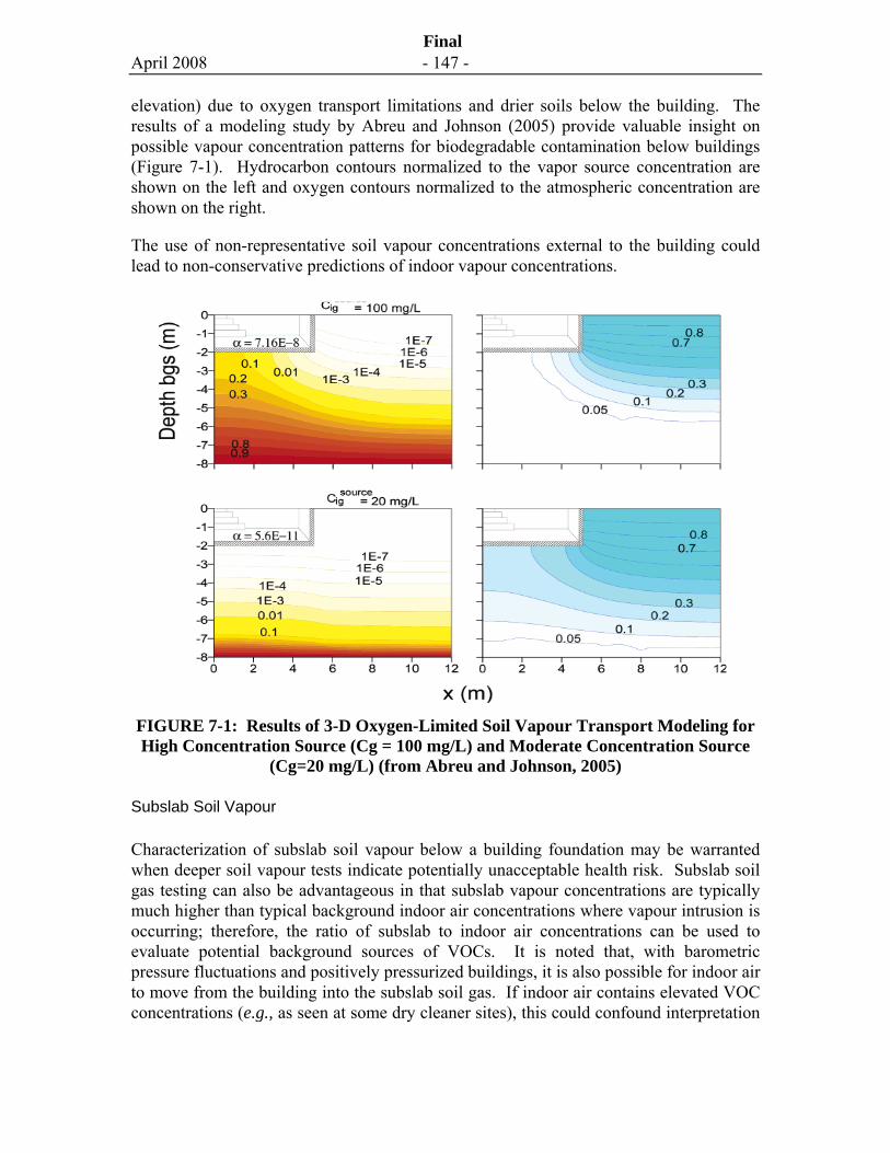
April 2008 - 147 -

Final

elevation) due to oxygen transport limitations and drier soils below the building. The results of a modeling study by Abreu and Johnson (2005) provide valuable insight on possible vapour concentration patterns for biodegradable contamination below buildings (Figure 7-1). Hydrocarbon contours normalized to the vapor source concentration are shown on the left and oxygen contours normalized to the atmospheric concentration are shown on the right.

The use of non-representative soil vapour concentrations external to the building could lead to non-conservative predictions of indoor vapour concentrations.

FIGURE 7-1: Results of 3-D Oxygen-Limited Soil Vapour Transport Modeling for High Concentration Source (Cg = 100 mg/L) and Moderate Concentration Source

(Cg=20 mg/L) (from Abreu and Johnson, 2005) Subslab Soil Vapour

Characterization of subslab soil vapour below a building foundation may be warranted when deeper soil vapour tests indicate potentially unacceptable health risk. Subslab soil gas testing can also be advantageous in that subslab vapour concentrations are typically much higher than typical background indoor air concentrations where vapour intrusion is occurring; therefore, the ratio of subslab to indoor air concentrations can be used to evaluate potential background sources of VOCs. It is noted that, with barometric pressure fluctuations and positively pressurized buildings, it is also possible for indoor air to move from the building into the subslab soil gas. If indoor air contains elevated VOC concentrations (e.g., as seen at some dry cleaner sites), this could confound interpretation

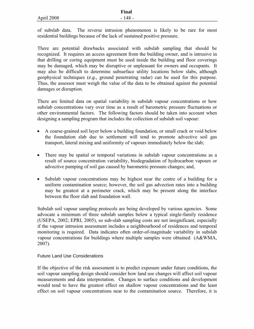
April 2008 - 148 -

Final

of subslab data. The reverse intrusion phenomenon is likely to be rare for most residential buildings because of the lack of sustained positive pressure.

There are potential drawbacks associated with subslab sampling that should be recognized. It requires an access agreement from the building owner, and is intrusive in that drilling or coring equipment must be used inside the building and floor coverings may be damaged, which may be disruptive or unpleasant for owners and occupants. It may also be difficult to determine subsurface utility locations below slabs, although geophysical techniques (e.g., ground penetrating radar) can be used for this purpose. Thus, the assessor must weigh the value of the data to be obtained against the potential damages or disruption.

There are limited data on spatial variability in subslab vapour concentrations or how subslab concentrations vary over time as a result of barometric pressure fluctuations or other environmental factors. The following factors should be taken into account when designing a sampling program that includes the collection of subslab soil vapour:

• A coarse-grained soil layer below a building foundation, or small crack or void below the foundation slab due to settlement will tend to promote advective soil gas transport, lateral mixing and uniformity of vapours immediately below the slab;

• There may be spatial or temporal variations in subslab vapour concentrations as a result of source concentration variability, biodegradation of hydrocarbon vapours or advective pumping of soil gas caused by barometric pressure changes; and,

• Subslab vapour concentrations may be highest near the centre of a building for a uniform contamination source; however, the soil gas advection rates into a building may be greatest at a perimeter crack, which may be present along the interface between the floor slab and foundation wall.

Subslab soil vapour sampling protocols are being developed by various agencies. Some advocate a minimum of three subslab samples below a typical single-family residence (USEPA, 2002; EPRI, 2005), so sub-slab sampling costs are not insignificant, especially if the vapour intrusion assessment includes a neighbourhood of residences and temporal monitoring is required. Data indicates often order-of-magnitude variability in subslab vapour concentrations for buildings where multiple samples were obtained (A&WMA, 2007).

Future Land Use Considerations

If the objective of the risk assessment is to predict exposure under future conditions, the soil vapour sampling design should consider how land use changes will affect soil vapour measurements and data interpretation. Changes to surface conditions and development would tend to have the greatest effect on shallow vapour concentrations and the least effect on soil vapour concentrations near to the contamination source. Therefore, it is

April 2008 - 149 -

Final

recommended that soil vapour characterization programs for the future use scenario ensure that sampling of deep near source soil gas is included as part of the soil vapour sampling program.

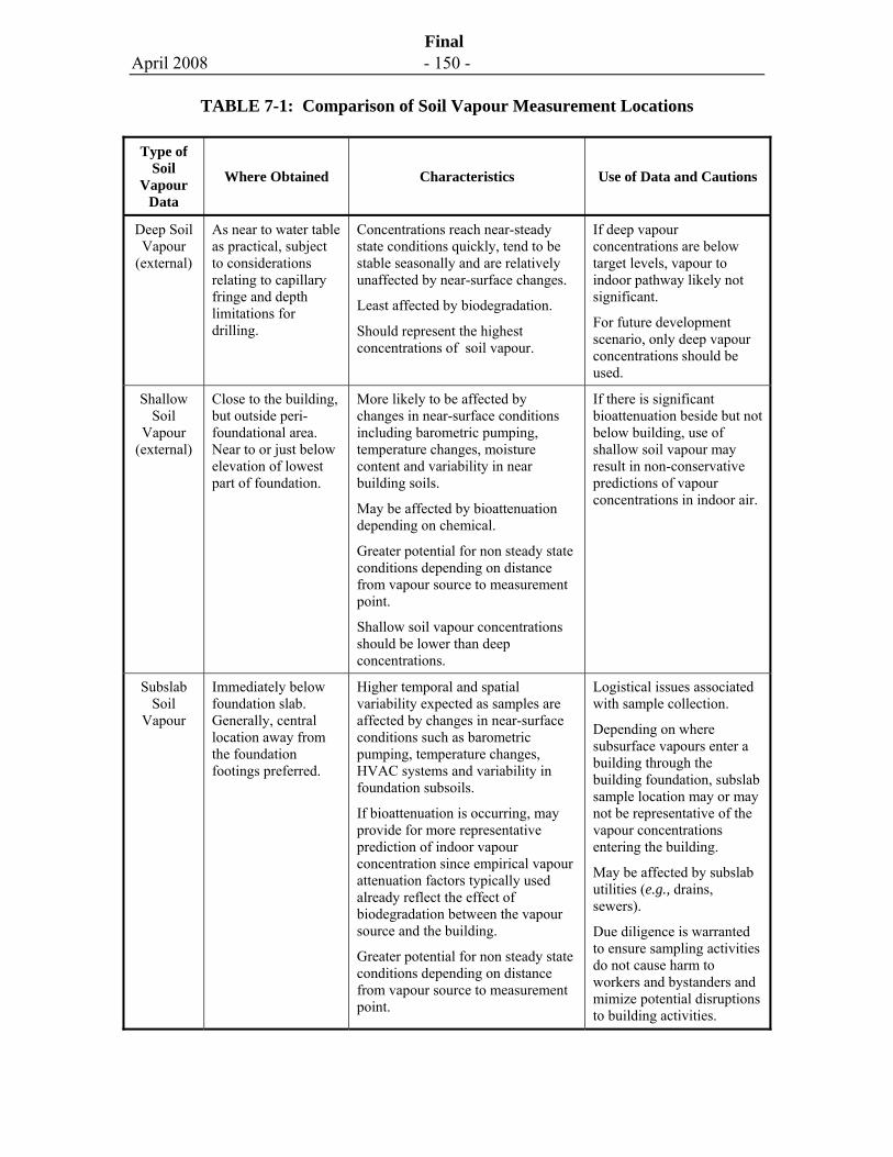
April 2008 - 150 -

Final

TABLE 7-1: Comparison of Soil Vapour Measurement Locations

Type of Soil

Vapour Data

Where Obtained Characteristics Use of Data and Cautions

Deep Soil Vapour

(external)

As near to water table as practical, subject to considerations relating to capillary fringe and depth limitations for drilling.

Concentrations reach near-steady state conditions quickly, tend to be stable seasonally and are relatively unaffected by near-surface changes.

Least affected by biodegradation.

Should represent the highest concentrations of soil vapour.

If deep vapour concentrations are below target levels, vapour to indoor pathway likely not significant.

For future development scenario, only deep vapour concentrations should be used.

Shallow Soil

Vapour (external)

Close to the building, but outside peri-foundational area. Near to or just below elevation of lowest part of foundation.

More likely to be affected by changes in near-surface conditions including barometric pumping, temperature changes, moisture content and variability in near building soils.

May be affected by bioattenuation depending on chemical.

Greater potential for non steady state conditions depending on distance from vapour source to measurement point.

Shallow soil vapour concentrations should be lower than deep concentrations.

If there is significant bioattenuation beside but not below building, use of shallow soil vapour may result in non-conservative predictions of vapour concentrations in indoor air.

Subslab Soil

Vapour

Immediately below foundation slab. Generally, central location away from the foundation footings preferred.

Higher temporal and spatial variability expected as samples are affected by changes in near-surface conditions such as barometric pumping, temperature changes, HVAC systems and variability in foundation subsoils.

If bioattenuation is occurring, may provide for more representative prediction of indoor vapour concentration since empirical vapour attenuation factors typically used already reflect the effect of biodegradation between the vapour source and the building.

Greater potential for non steady state conditions depending on distance from vapour source to measurement point.

Logistical issues associated with sample collection.

Depending on where subsurface vapours enter a building through the building foundation, subslab sample location may or may not be representative of the vapour concentrations entering the building.

May be affected by subslab utilities (e.g., drains, sewers).

Due diligence is warranted to ensure sampling activities do not cause harm to workers and bystanders and mimize potential disruptions to building activities.

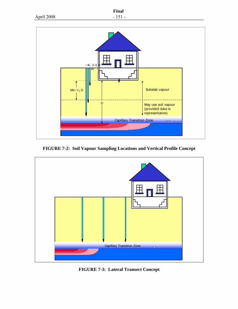
April 2008 - 151 -

Final

FIGURE 7-2: Soil Vapour Sampling Locations and Vertical Profile Concept

FIGURE 7-3: Lateral Transect Concept

Capillary Transition Zone

2-3 m

Min 1/2 D

Capillary Transition Zone

May use soil vapour(provided data is representative)

Subslab vapour

D

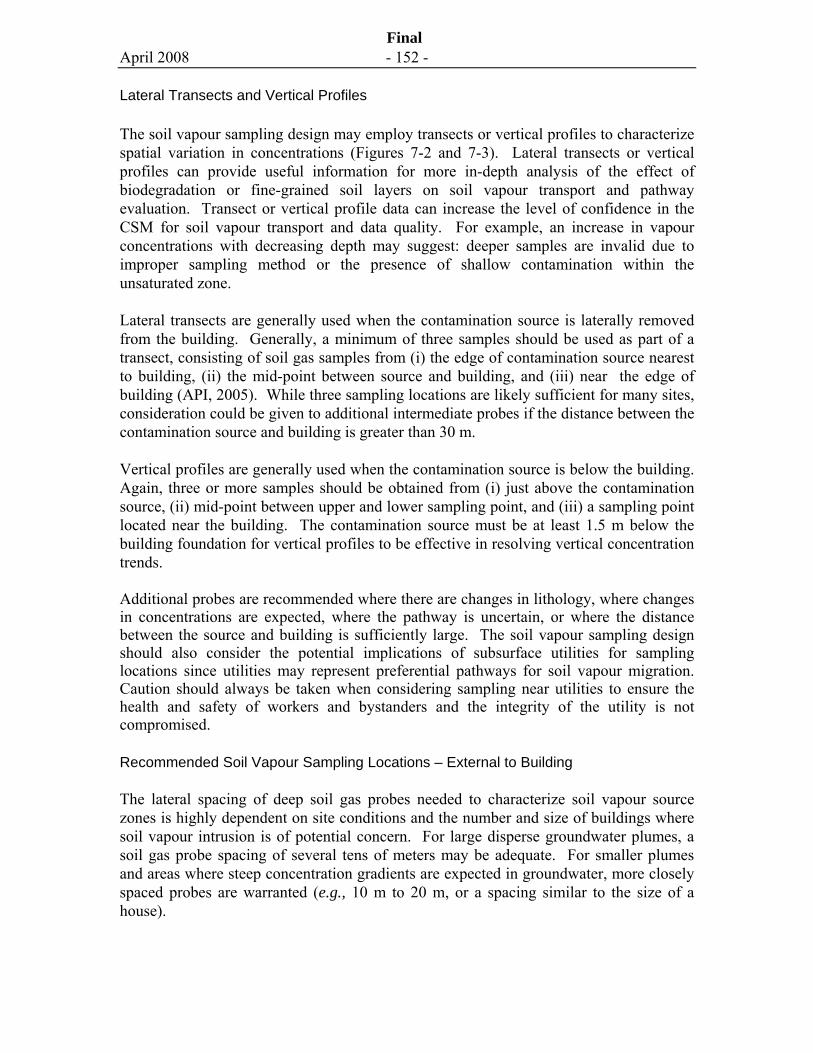
April 2008 - 152 -

Final

Lateral Transects and Vertical Profiles

The soil vapour sampling design may employ transects or vertical profiles to characterize spatial variation in concentrations (Figures 7-2 and 7-3). Lateral transects or vertical profiles can provide useful information for more in-depth analysis of the effect of biodegradation or fine-grained soil layers on soil vapour transport and pathway evaluation. Transect or vertical profile data can increase the level of confidence in the CSM for soil vapour transport and data quality. For example, an increase in vapour concentrations with decreasing depth may suggest: deeper samples are invalid due to improper sampling method or the presence of shallow contamination within the unsaturated zone.

Lateral transects are generally used when the contamination source is laterally removed from the building. Generally, a minimum of three samples should be used as part of a transect, consisting of soil gas samples from (i) the edge of contamination source nearest to building, (ii) the mid-point between source and building, and (iii) near the edge of building (API, 2005). While three sampling locations are likely sufficient for many sites, consideration could be given to additional intermediate probes if the distance between the contamination source and building is greater than 30 m.

Vertical profiles are generally used when the contamination source is below the building. Again, three or more samples should be obtained from (i) just above the contamination source, (ii) mid-point between upper and lower sampling point, and (iii) a sampling point located near the building. The contamination source must be at least 1.5 m below the building foundation for vertical profiles to be effective in resolving vertical concentration trends.

Additional probes are recommended where there are changes in lithology, where changes in concentrations are expected, where the pathway is uncertain, or where the distance between the source and building is sufficiently large. The soil vapour sampling design should also consider the potential implications of subsurface utilities for sampling locations since utilities may represent preferential pathways for soil vapour migration. Caution should always be taken when considering sampling near utilities to ensure the health and safety of workers and bystanders and the integrity of the utility is not compromised.

Recommended Soil Vapour Sampling Locations – External to Building

The lateral spacing of deep soil gas probes needed to characterize soil vapour source zones is highly dependent on site conditions and the number and size of buildings where soil vapour intrusion is of potential concern. For large disperse groundwater plumes, a soil gas probe spacing of several tens of meters may be adequate. For smaller plumes and areas where steep concentration gradients are expected in groundwater, more closely spaced probes are warranted (e.g., 10 m to 20 m, or a spacing similar to the size of a house).

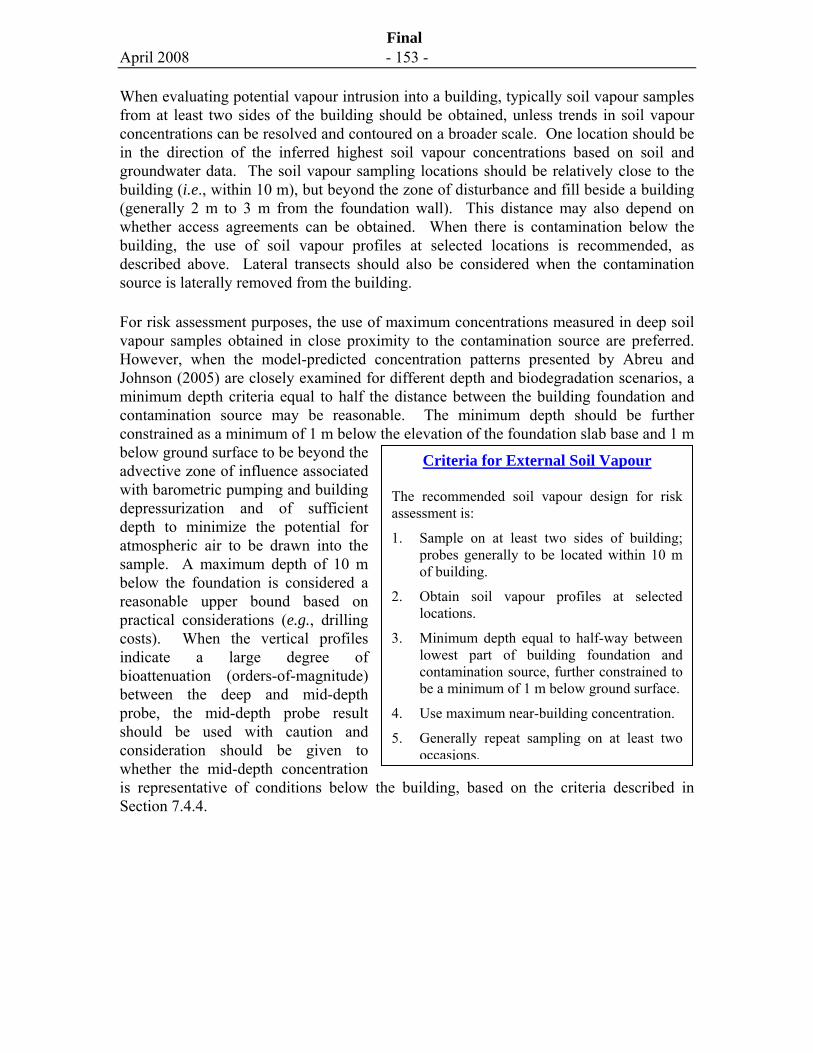
April 2008 - 153 -

Final

Criteria for External Soil Vapour

The recommended soil vapour design for risk assessment is:

1. Sample on at least two sides of building; probes generally to be located within 10 m of building.

2. Obtain soil vapour profiles at selected locations.

3. Minimum depth equal to half-way between lowest part of building foundation and contamination source, further constrained to be a minimum of 1 m below ground surface.

4. Use maximum near-building concentration.

5. Generally repeat sampling on at least two occasions.

When evaluating potential vapour intrusion into a building, typically soil vapour samples from at least two sides of the building should be obtained, unless trends in soil vapour concentrations can be resolved and contoured on a broader scale. One location should be in the direction of the inferred highest soil vapour concentrations based on soil and groundwater data. The soil vapour sampling locations should be relatively close to the building (i.e., within 10 m), but beyond the zone of disturbance and fill beside a building (generally 2 m to 3 m from the foundation wall). This distance may also depend on whether access agreements can be obtained. When there is contamination below the building, the use of soil vapour profiles at selected locations is recommended, as described above. Lateral transects should also be considered when the contamination source is laterally removed from the building.

For risk assessment purposes, the use of maximum concentrations measured in deep soil vapour samples obtained in close proximity to the contamination source are preferred. However, when the model-predicted concentration patterns presented by Abreu and Johnson (2005) are closely examined for different depth and biodegradation scenarios, a minimum depth criteria equal to half the distance between the building foundation and contamination source may be reasonable. The minimum depth should be further constrained as a minimum of 1 m below the elevation of the foundation slab base and 1 m below ground surface to be beyond the advective zone of influence associated with barometric pumping and building depressurization and of sufficient depth to minimize the potential for atmospheric air to be drawn into the sample. A maximum depth of 10 m below the foundation is considered a reasonable upper bound based on practical considerations (e.g., drilling costs). When the vertical profiles indicate a large degree of bioattenuation (orders-of-magnitude) between the deep and mid-depth probe, the mid-depth probe result should be used with caution and consideration should be given to whether the mid-depth concentration is representative of conditions below the building, based on the criteria described in Section 7.4.4.

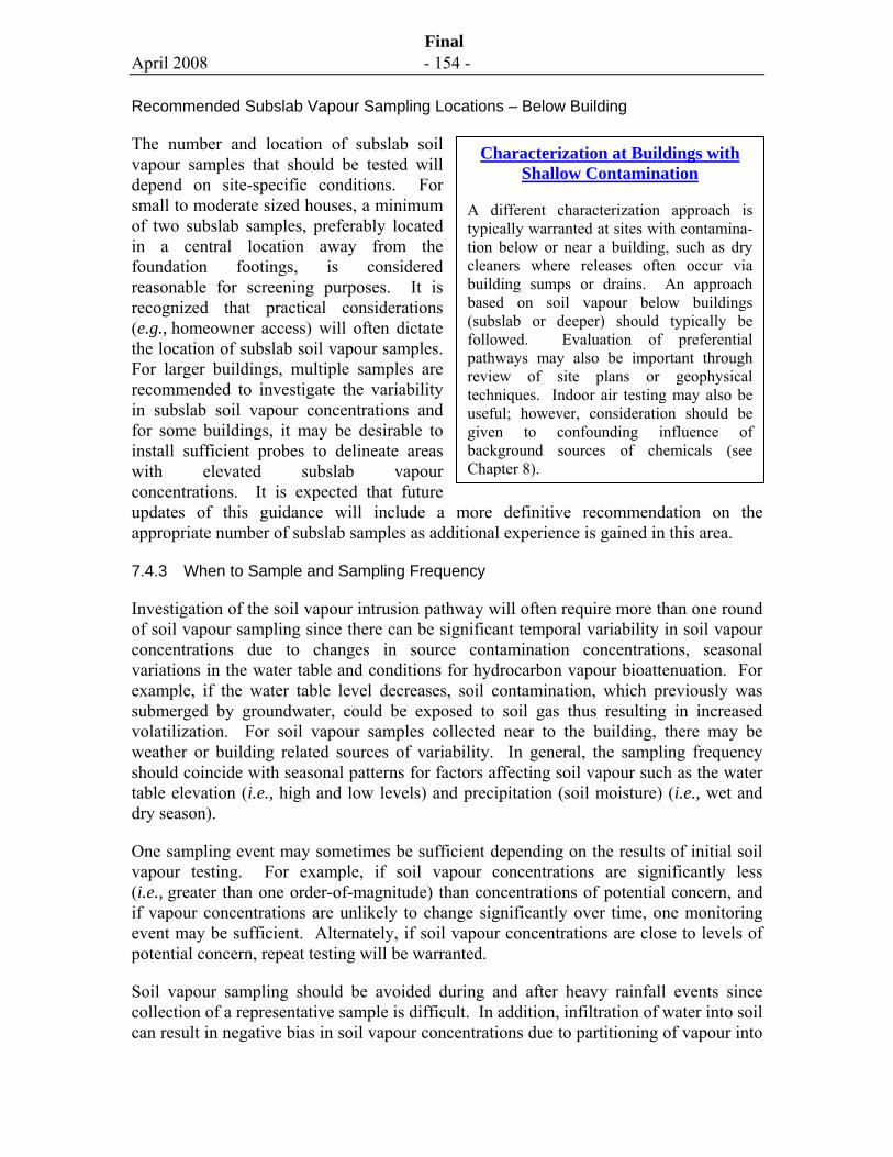
April 2008 - 154 -

Final

Recommended Subslab Vapour Sampling Locations – Below Building

The number and location of subslab soil vapour samples that should be tested will depend on site-specific conditions. For small to moderate sized houses, a minimum of two subslab samples, preferably located in a central location away from the foundation footings, is considered reasonable for screening purposes. It is recognized that practical considerations (e.g., homeowner access) will often dictate the location of subslab soil vapour samples. For larger buildings, multiple samples are recommended to investigate the variability in subslab soil vapour concentrations and for some buildings, it may be desirable to install sufficient probes to delineate areas with elevated subslab vapour concentrations. It is expected that future updates of this guidance will include a more definitive recommendation on the appropriate number of subslab samples as additional experience is gained in this area.

7.4.3 When to Sample and Sampling Frequency

Investigation of the soil vapour intrusion pathway will often require more than one round of soil vapour sampling since there can be significant temporal variability in soil vapour concentrations due to changes in source contamination concentrations, seasonal variations in the water table and conditions for hydrocarbon vapour bioattenuation. For example, if the water table level decreases, soil contamination, which previously was submerged by groundwater, could be exposed to soil gas thus resulting in increased volatilization. For soil vapour samples collected near to the building, there may be weather or building related sources of variability. In general, the sampling frequency should coincide with seasonal patterns for factors affecting soil vapour such as the water table elevation (i.e., high and low levels) and precipitation (soil moisture) (i.e., wet and dry season).

One sampling event may sometimes be sufficient depending on the results of initial soil vapour testing. For example, if soil vapour concentrations are significantly less (i.e., greater than one order-of-magnitude) than concentrations of potential concern, and if vapour concentrations are unlikely to change significantly over time, one monitoring event may be sufficient. Alternately, if soil vapour concentrations are close to levels of potential concern, repeat testing will be warranted.

Soil vapour sampling should be avoided during and after heavy rainfall events since collection of a representative sample is difficult. In addition, infiltration of water into soil can result in negative bias in soil vapour concentrations due to partitioning of vapour into

Characterization at Buildings with Shallow Contamination

A different characterization approach is typically warranted at sites with contamina-tion below or near a building, such as dry cleaners where releases often occur via building sumps or drains. An approach based on soil vapour below buildings (subslab or deeper) should typically be followed. Evaluation of preferential pathways may also be important through review of site plans or geophysical techniques. Indoor air testing may also be useful; however, consideration should be given to confounding influence of background sources of chemicals (see Chapter 8).

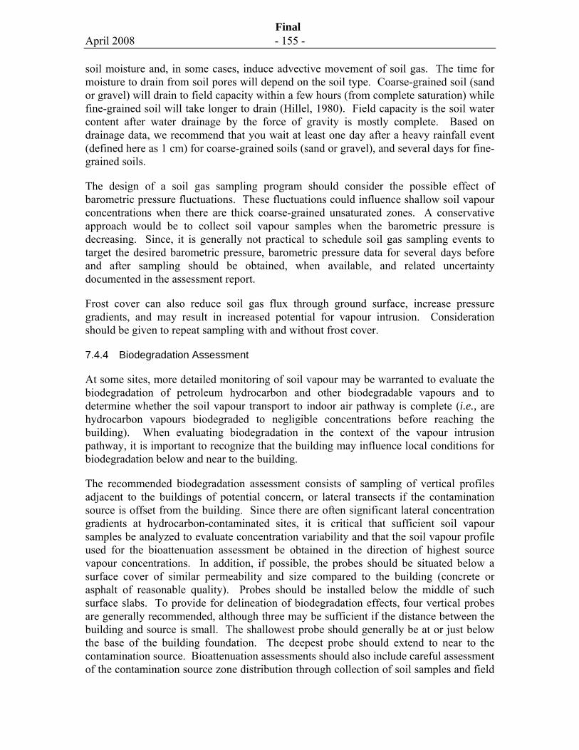
April 2008 - 155 -

Final

soil moisture and, in some cases, induce advective movement of soil gas. The time for moisture to drain from soil pores will depend on the soil type. Coarse-grained soil (sand or gravel) will drain to field capacity within a few hours (from complete saturation) while fine-grained soil will take longer to drain (Hillel, 1980). Field capacity is the soil water content after water drainage by the force of gravity is mostly complete. Based on drainage data, we recommend that you wait at least one day after a heavy rainfall event (defined here as 1 cm) for coarse-grained soils (sand or gravel), and several days for fine-grained soils.

The design of a soil gas sampling program should consider the possible effect of barometric pressure fluctuations. These fluctuations could influence shallow soil vapour concentrations when there are thick coarse-grained unsaturated zones. A conservative approach would be to collect soil vapour samples when the barometric pressure is decreasing. Since, it is generally not practical to schedule soil gas sampling events to target the desired barometric pressure, barometric pressure data for several days before and after sampling should be obtained, when available, and related uncertainty documented in the assessment report.

Frost cover can also reduce soil gas flux through ground surface, increase pressure gradients, and may result in increased potential for vapour intrusion. Consideration should be given to repeat sampling with and without frost cover.

7.4.4 Biodegradation Assessment

At some sites, more detailed monitoring of soil vapour may be warranted to evaluate the biodegradation of petroleum hydrocarbon and other biodegradable vapours and to determine whether the soil vapour transport to indoor air pathway is complete (i.e., are hydrocarbon vapours biodegraded to negligible concentrations before reaching the building). When evaluating biodegradation in the context of the vapour intrusion pathway, it is important to recognize that the building may influence local conditions for biodegradation below and near to the building.

The recommended biodegradation assessment consists of sampling of vertical profiles adjacent to the buildings of potential concern, or lateral transects if the contamination source is offset from the building. Since there are often significant lateral concentration gradients at hydrocarbon-contaminated sites, it is critical that sufficient soil vapour samples be analyzed to evaluate concentration variability and that the soil vapour profile used for the bioattenuation assessment be obtained in the direction of highest source vapour concentrations. In addition, if possible, the probes should be situated below a surface cover of similar permeability and size compared to the building (concrete or asphalt of reasonable quality). Probes should be installed below the middle of such surface slabs. To provide for delineation of biodegradation effects, four vertical probes are generally recommended, although three may be sufficient if the distance between the building and source is small. The shallowest probe should generally be at or just below the base of the building foundation. The deepest probe should extend to near to the contamination source. Bioattenuation assessments should also include careful assessment of the contamination source zone distribution through collection of soil samples and field

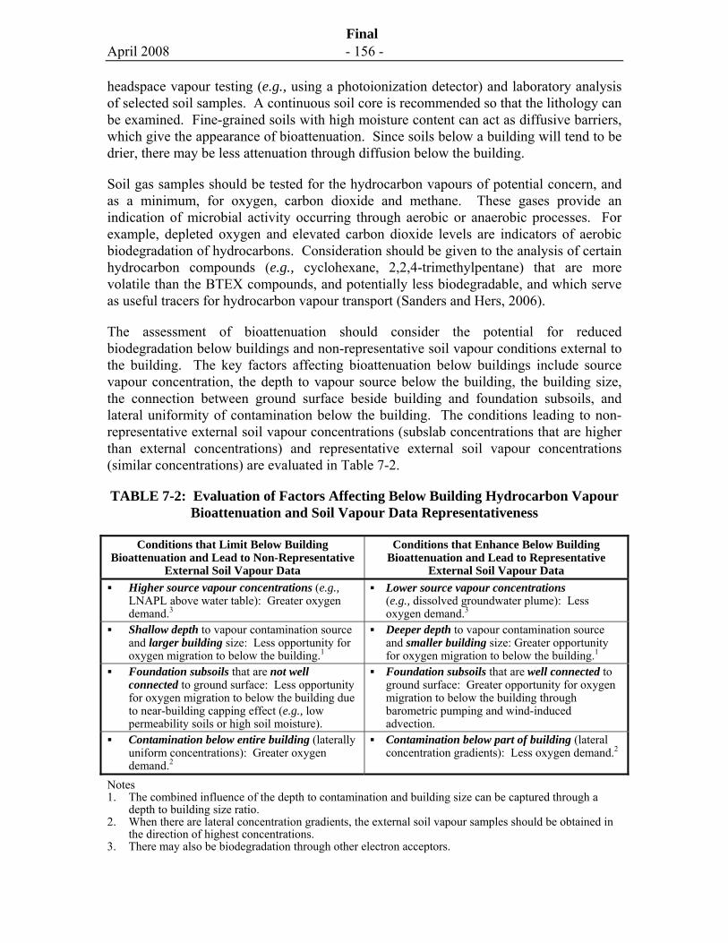
April 2008 - 156 -

Final

headspace vapour testing (e.g., using a photoionization detector) and laboratory analysis of selected soil samples. A continuous soil core is recommended so that the lithology can be examined. Fine-grained soils with high moisture content can act as diffusive barriers, which give the appearance of bioattenuation. Since soils below a building will tend to be drier, there may be less attenuation through diffusion below the building.

Soil gas samples should be tested for the hydrocarbon vapours of potential concern, and as a minimum, for oxygen, carbon dioxide and methane. These gases provide an indication of microbial activity occurring through aerobic or anaerobic processes. For example, depleted oxygen and elevated carbon dioxide levels are indicators of aerobic biodegradation of hydrocarbons. Consideration should be given to the analysis of certain hydrocarbon compounds (e.g., cyclohexane, 2,2,4-trimethylpentane) that are more volatile than the BTEX compounds, and potentially less biodegradable, and which serve as useful tracers for hydrocarbon vapour transport (Sanders and Hers, 2006).

The assessment of bioattenuation should consider the potential for reduced biodegradation below buildings and non-representative soil vapour conditions external to the building. The key factors affecting bioattenuation below buildings include source vapour concentration, the depth to vapour source below the building, the building size, the connection between ground surface beside building and foundation subsoils, and lateral uniformity of contamination below the building. The conditions leading to non-representative external soil vapour concentrations (subslab concentrations that are higher than external concentrations) and representative external soil vapour concentrations (similar concentrations) are evaluated in Table 7-2.

TABLE 7-2: Evaluation of Factors Affecting Below Building Hydrocarbon Vapour Bioattenuation and Soil Vapour Data Representativeness

Conditions that Limit Below Building Bioattenuation and Lead to Non-Representative

External Soil Vapour Data

Conditions that Enhance Below Building Bioattenuation and Lead to Representative

External Soil Vapour Data Higher source vapour concentrations (e.g.,

LNAPL above water table): Greater oxygen demand.3

Lower source vapour concentrations (e.g., dissolved groundwater plume): Less oxygen demand.3

Shallow depth to vapour contamination source and larger building size: Less opportunity for oxygen migration to below the building.1

Deeper depth to vapour contamination source and smaller building size: Greater opportunity for oxygen migration to below the building.1

Foundation subsoils that are not well connected to ground surface: Less opportunity for oxygen migration to below the building due to near-building capping effect (e.g., low permeability soils or high soil moisture).

Foundation subsoils that are well connected to ground surface: Greater opportunity for oxygen migration to below the building through barometric pumping and wind-induced advection.

Contamination below entire building (laterally uniform concentrations): Greater oxygen demand.2

Contamination below part of building (lateral concentration gradients): Less oxygen demand.2

Notes 1. The combined influence of the depth to contamination and building size can be captured through a

depth to building size ratio. 2. When there are lateral concentration gradients, the external soil vapour samples should be obtained in

the direction of highest concentrations. 3. There may also be biodegradation through other electron acceptors.

April 2008 - 157 -

Final

The above qualitative factors should be reviewed when evaluating the use of external soil vapour data. If conditions suggest shallow data may not be representative, then it is recommended that deep soil vapour data be used for assessment purposes. Alternately, consideration could be given to sampling and analysis of subslab soil vapour samples to confirm that bioattenuation is also occurring below the building. If multiple buildings are potentially affected, testing below a subset of building(s) in the highest source concentration area may be sufficient to demonstrate bioattenuation is occurring.

Hydrocarbon vapour biodegradation is an area of active research. It is expected that more quantitative guidance on how to apply dilution factors to account for biodegradation will be developed over the next few years.

7.5 Soil Gas Probe Construction and Installation

Soil gas probes can be constructed of a variety of materials and installed using several techniques (EPRI, 2005; API; 2005; Atlantic PIRI, 2006). Critical aspects to probe construction include (i) probes should be constructed from materials that are relatively inert and non-sorptive, (ii) techniques should be used to minimize the potential for short-circuiting of atmospheric air to the probe soil gas collection point, and (iii) the probe should remain sealed between sampling events. The main options for installation of soil gas probes include:

• Probes installed in boreholes in soil or coreholes through a concrete slab; • Probes installed via direct push technology; and, • Driven probes.

Further discussion on the probe materials and installation methods for each of the above probe types is described below. For all probe types, it is important that subsurface utilities be located prior to installation. Multiple options for probes are described to provide the practitioner with alternatives to accommodate site-specific conditions and constraints (see SOP #4).

7.5.1 Probes Installed in Boreholes

Probes installed in boreholes are constructed in a similar fashion to groundwater monitoring wells; however, there are important differences in design. Generally short screens (0.1 m to 0.3 m length) should be used for probes since typically the objective is to characterize local soil gas concentrations (i.e., over a small volume). The probe diameter should be kept small (maximum of 25 mm (1 inch) and preferably less) to minimize purge volumes and surface area for adsorption of VOCs on probe surfaces.

Two common probe designs are rigid PVC pipe and “implants” constructed of steel mesh screens connected to flexible tubing. For probes constructed of continuous PVC pipe to ground surface, 19 mm (¾ inch) diameter pipe is recommended. While the slot size for groundwater wells is typically No. 10 slot (0.01 inch), a larger slot size (up to No. 40

April 2008 - 158 -

Final

slot) may be used for PVC soil gas probes since there is less potential for the filter pack to intrude into the probe within the unsaturated zone. Commercially-available implants are typically 0.15 m to 0.3 m long, 12.5 mm (½ inch) in diameter, and connected to ground surface using 6 mm (¼ inch) tubing. A potential disadvantage of smaller diameter tubing (i.e., 6 mm or smaller) is frictional losses if pneumatic tests are to be performed (see SOP #5). A threaded cap should be placed over top of the riser pipe and riser pipe segments should be flush-threaded. No glue should be used for construction of probes.

Coarse sand or fine gravel should be placed surrounding the screened portion of the probe, and a bentonite seal (minimum 0.3 m thick) should be constructed above the screened portion of the probe. Since soil gas probes are installed in the unsaturated zone where soil moisture may be relatively low, careful consideration should be given to the hydration of the bentonite seal. A competent seal can be constructed through use of dry granular bentonite (16 mesh), as opposed to powder, chips, or pellets, and addition of distilled water to the bentonite during installation. Granular bentonite has a texture much like the sand used for a filter-pack, and so it will settle effectively within the borehole, but hydrates instantaneously. Two or three lifts of granular bentonite and water is usually sufficient to form a competent seal. An effective method of sealing the remainder of the borehole annulus is to use a thick slurry of powdered bentonite and water (“volclay grout”). At some sites, it may be prudent to use distilled water for hydration to avoid compromising soil gas with volatiles commonly detected in tap water (e.g. chloroform).

If multiple probes are installed in a single borehole, the borehole above and below each probe should be sealed with granular bentonite. After allowing the seal to set overnight, the integrity of the seal should be checked by drawing a vacuum on each probe, and measuring the vacuum at adjacent probes. For a competent seal, a vacuum may still be measured at adjacent probes; however, the vacuum will develop slowly and will be less than that measured at the pumped probe (EPRI, 2005). Soil gas probes should be completed with an air-tight valve or stopcock at surface to prevent atmospheric air from entering the probe, and protected using a well cover or other similar protective casing for security and weatherproofing. If multi-level probes are used, each probe should be tagged with a permanent label, using no glues or markers. In general, a similar or higher level of care and quality control to that employed for monitoring wells should be followed when installing a soil gas probe.

Potential advantages of permanent probes installed in boreholes are that temporal variability can be assessed through repeat sampling and there is greater installation flexibility (i.e., deep probes, dense soils). In addition, the filter pack that surrounds the screen provides for more open area for drawing a soil gas sample than a driven probe. A potential disadvantage of probes installed in boreholes may be access restrictions for drill rigs.

Soil samples should be collected during drilling of boreholes for soil gas probes. Consideration should be given to testing of soil samples for soil moisture content and grain size distribution and the soil lithology and stratigraphy should be carefully logged.

April 2008 - 159 -

Final

Soil samples should also be evaluated for possible contamination, including sources that may be located above the water table (see Section 7.8).

7.5.2 Probes Installed Using Direct Push Technology

Direct-push techniques can be used to install a single soil gas implant in a borehole. Direct push rods are pushed to the desired depth, and implants are installed post-run after the desired depth is reached by lowering the implant down the hollow rods and attaching it to a detachable anchor drive point. A sand pack and bentonite seal should be installed through the push rods as they are removed to minimize the potential for short-circuiting of atmospheric air from ground surface to the sampling point. The position of the filter pack and seal should be confirmed using a tamping rod. It is noted that past practice has been that installers often relied on the natural collapse of the formation around the probes; however, this technique will not provide a competent seal and should not be relied upon.

There is also direct push equipment that enables collection of multiple depth samples during a single push where soil gas samples are collected through a screen located within a retractable protective sleeve. This technology may be useful in characterizing soil vapour concentrations above source contamination zones; however, due to the potential for cross-contamination, it should not be used within or below source contamination zones.

A potential advantage of using direct push technology to install a probe is that implants can be rapidly installed with minimal disturbance. A potential disadvantage is short-circuiting of atmospheric air from surface to the sampling point, if the borehole above the screen is not well sealed. In addition, the presence of gravel or cobbles may hinder or preclude the use of direct-push technology.

7.5.3 Driven Probes

Driven probes in their simplest form are hollow steel rods with an internal diameter typically ranging between 9 mm and 25 mm (sometimes referred to as ground probes). The probes can be driven by hand, or with the aid of direct push equipped vehicles. The rods include a loosely-fitting conical tip that is pushed a short distance further into the formation using an inner rod, once the probe is driven to its desired depth. Several holes may also be drilled near the tip of the probe to increase the open area through which soil gas is drawn into the probe. Driven probes are often temporary installations in that the probe is removed after the sample is obtained.

Driven probes may be advantageous in terms of flexibility of installation and cost. Another potential advantage is that when field analytical capabilities are available, multiple soil gas samples may be collected and analyzed from a single driven probe installed to varying depths enabling near real-time evaluation of vertical vapour profiles. One disadvantage is that driven probes can be difficult to install in coarse-grained or dense soil, especially at greater depths. The use of driven probes is discouraged in low permeability soils as it is difficult to ensure the absence of annular leakage, which is more

April 2008 - 160 -

Final

likely to become a path of least resistance in low permeability soils. As described in SOP #6, tracer tests (e.g., using helium) are recommended to evaluate possible annular leakage along the outside of driven probes.

7.5.4 Use of Water Table Monitoring Wells as Soil Gas Probes

Soil gas samples can also be obtained from groundwater monitoring wells screened across the water table provided the well screen extends above the capillary fringe. Prior to collecting a sample for analysis, the well should be purged by removing several casing volumes of air. For typical well diameters, a purge rate of several litres per minute may be required, and therefore an appropriate sized pump is required for this approach. Since groundwater wells may be vented at surface, an air-tight cap and valve should be used when sampling soil gas.

Since essentially a composite soil gas sample is obtained over the length of the well screen above the capillary fringe, data from monitoring wells may not provide the desired vertical discretization. Off-gasing of volatiles from groundwater at the water table surface and from the capillary fringe will influence the soil vapour concentrations to varying degrees. For a thick capillary fringe, the surface area over which volatilization could occur within the well may be significant (approaching 1 m2). For this scenario, the soil vapour concentration measured in a monitoring well may be significantly higher than that measured in a soil gas probe installed directly above the capillary fringe, meaning that data from wells may be unsuitable for evaluation of concentration attenuation within the capillary transition zone. Borehole logs for the area should be consulted, and vapour monitors installed above indications of the capillary fringe.

7.5.5 Subslab Soil Gas Probes

Prior to drilling or coring through concrete slabs, relevant structural and utility information should be reviewed to evaluate whether drilling or coring could adversely affect the integrity of the building envelope, foundation slab or subsurface utilities, and whether there are any potential health and safety issues with drilling or coring. As warranted, geophysical techniques should be used to identify the location of re-bar within concrete slabs prior to drilling. After drilling the hole and prior to installation of the probe, the hole should be temporarily sealed (e.g., using a rubber stopper) to minimize disturbance to subslab vapour concentrations.

Typically, the objective of subslab soil gas sampling is to characterize vapour concentrations in foundation subsoils immediately below the slab. Therefore, permanent probes typically consist of stainless steel or brass inserts installed within a corehole that are sealed with concrete grout (USEPA, 2004). The concrete grout should consist of Portland cement, aggregate and water, and should not contain any additives that could contain VOCs. A fast setting, hydrating (swelling) cement may be a good option provided there are no additives that give off VOCs. A subslab probe design by USEPA (2004) is shown in Figure 7-4.

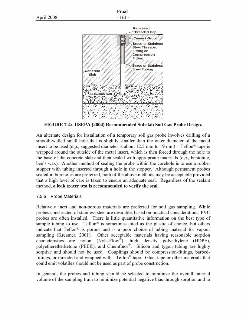
April 2008 - 161 -

Final

FIGURE 7-4: USEPA (2004) Recommended Subslab Soil Gas Probe Design.

An alternate design for installation of a temporary soil gas probe involves drilling of a smooth-walled small hole that is slightly smaller than the outer diameter of the metal insert to be used (e.g., suggested diameter is about 12.5 mm to 19 mm) . Teflon®-tape is wrapped around the outside of the metal insert, which is then forced through the hole to the base of the concrete slab and then sealed with appropriate materials (e.g., bentonite, bee’s wax). Another method of sealing the probe within the corehole is to use a rubber stopper with tubing inserted through a hole in the stopper. Although permanent probes sealed in boreholes are preferred, both of the above methods may be acceptable provided that a high level of care is taken to ensure an adequate seal. Regardless of the sealant method, a leak tracer test is recommended to verify the seal.

7.5.6 Probe Materials

Relatively inert and non-porous materials are preferred for soil gas sampling. While probes constructed of stainless steel are desirable, based on practical considerations, PVC probes are often installed. There is little quantitative information on the best type of sample tubing to use. Teflon® is sometimes cited as the plastic of choice, but others indicate that Teflon® is porous and is a poor choice of tubing material for vapour sampling (Kreamer, 2001). Other acceptable materials having reasonable sorption characteristics are nylon (Nyla-Flow®), high density polyethylene (HDPE), polyetheretherketone (PEEK), and Chemfluor®. Silicon and tygon tubing are highly sorptive and should not be used. Couplings should be compression-fittings, barbed-fittings, or threaded and wrapped with Teflon® tape. Glue, tape or other materials that could emit volatiles should not be used as part of probe construction.

In general, the probes and tubing should be selected to minimize the overall internal volume of the sampling train to minimize potential negative bias through sorption and to

April 2008 - 162 -

Final

minimize purge volumes. Sampling trains should be kept simple and tubing external to the probe should be kept as short as possible.

Only new materials should be used, except when temporary steel probes are re-used. Steel probes should be decontaminated prior to use. Care should be taken when storing and handling probe material to avoid contamination. Sampling and decontamination procedures should be documented as part of the QA/QC program.

7.5.7 Short-Circuiting Considerations

Short-circuiting of atmospheric air to the probe can occur between the probe and soil, and leakage of soil gas and/or atmospheric air can occur at probe joints. Prevention of short-circuiting and leaks is particularly important for low permeability soil deposits.

For finer-grained soils, the process of driving a steel probe may cause movement and cracking of soil around the probe, and hence the potential for short-circuiting during sampling. For driven probes, the surface surrounding the probe should be sealed with bentonite prior to sampling, or suitable alternate material that is inert (e.g., modeling clay) and the seal verified to be competent.

As discussed in SOP #6, the probe surface seal integrity may be tested by introducing a tracer gas (e.g., helium) around the probe at the contact with the ground surface and then analyzing the collected soil gas samples for the tracer gas. It is important to avoid the lateral or vertical movement of probes once installed to minimize any separation between the soils and the outer surface of the probes.

7.6 Soil Gas Sampling Procedures

Soil gas sampling procedures addressed in this section are soil gas equilibration, probe performance testing, sampling containers, decontamination, methods to detect leaks and short-circuiting, and purging and sampling. The methods used should be documented throughout the sampling process. Suggested Operating Procedure #5 provides additional details on soil gas sampling procedures. A good overview of sampling procedures is also provided in Atlantic PIRI (2006), API (2005) and EPRI (2005).

7.6.1 Probe Development and Soil Gas Equilibration

Soil gas probes should be developed and then allowed to equilibrate prior to sampling. Three probe volumes of air should be removed during development. The development process also facilitates the “conditioning” of the probe to soil vapour and filling of possible sorption sites. The time required for equilibration will depend on the disturbance caused during installation. The least disturbance is caused by driven probes, or probes installed using direct-push technology. Moderate disturbance is caused by auger drilling while the greatest disturbance is caused by air rotary drilling, since air is introduced into the formation during drilling. For driven probes or probes installed using

April 2008 - 163 -

Final

direct-push technology, a few minutes to hours is likely sufficient for equilibration of soil vapour concentrations (Diguilio et al., 2006). For probes installed in auger boreholes, a day or two may be sufficient. For air rotary boreholes, it may take several weeks for equilibration of soil vapour concentrations since air is used as a drilling fluid. For probes installed using air rotary drilling, it is recommended that repeat monitoring be conducted over several weeks to evaluate whether soil vapour concentrations surrounding the probe have recovered.

7.6.2 Flow and Vacuum (Probe Performance) Check

The performance testing of selected probes should be conducted prior to soil gas sampling. The objective of the performance test is to verify the flow and vacuum are within acceptable ranges prior to sampling. The test is conducted by withdrawing soil gas from the probe at the desired flow rate using a pump and measuring the vacuum. If the vacuum exceeds 0.18 psi (5” of water), a lower flow rate should be used to reduce the vacuum, where practical. Flow and vacuum measurements may also be used to estimate the soil-air permeability using mathematical models for soil gas flow to a point probe (Garbesi et al., 1995) or to a well (Johnson et al., 1990) (see SOP #5). For subslab soil gas samples, a lower vacuum (less than 1 inch of water) would typically be expected since granular materials are commonly present below foundation slabs.

Since pumping from probes causes a local disequilibrium, the volume removed from the well during the performance test should be minimized. As a rough rule-of-thumb, a wait time of two minutes for every 1 litre of soil gas removed is recommended between performance testing and sample collection. For sequencing of work, consideration should be given to performance testing and collection of soil gas samples for field screening at least one day prior to collection of samples for laboratory analysis.

7.6.3 Sampling Container or Device

Sample collection devices can include evacuated steel canisters, sorbent tubes, glass cylinders and Tedlar® bags2. The selection of a collection device is influenced by investigation objectives, analytical requirements and detection limits. For field screening using hand-held detectors, soil gas samples are often collected using Tedlar® bags. The use of vacuum chamber (“lung box”) to fill Tedlar® bags avoids passing soil gas through a pump and possible pump contamination that may result. Gas-tight syringes are often used for on-site analysis using mobile laboratories. Soil gas samples collected for analysis by a fixed laboratory for VOCs should generally be obtained using sorbent tubes or stainless steel (e.g., SummaTM) or glass-lined (e.g., SilcoSteelTM) canisters. Glass cylinders or Tedlar® bags may be appropriate for light gas analysis (oxygen, carbon dioxide, methane). Sampling devices are compared in Table 7-3.

2 TedlarTM is a proprietary plastic with properties similar to TeflonTM.

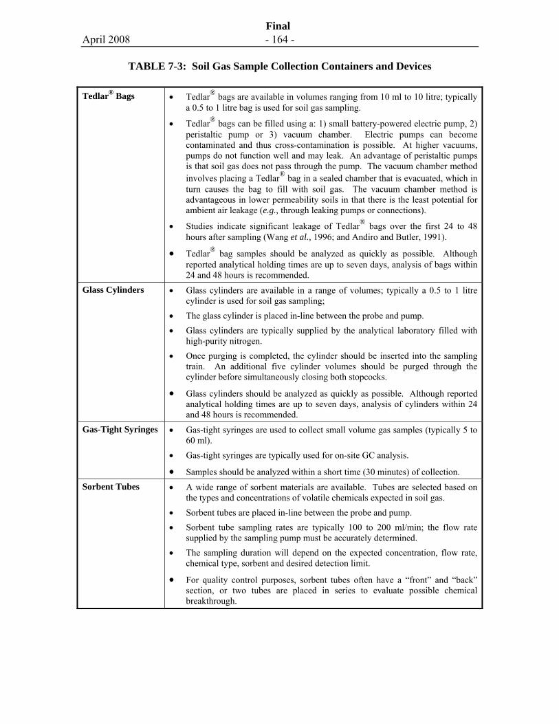
April 2008 - 164 -

Final

TABLE 7-3: Soil Gas Sample Collection Containers and Devices

Tedlar® Bags • Tedlar® bags are available in volumes ranging from 10 ml to 10 litre; typically a 0.5 to 1 litre bag is used for soil gas sampling.

• Tedlar® bags can be filled using a: 1) small battery-powered electric pump, 2) peristaltic pump or 3) vacuum chamber. Electric pumps can become contaminated and thus cross-contamination is possible. At higher vacuums, pumps do not function well and may leak. An advantage of peristaltic pumps is that soil gas does not pass through the pump. The vacuum chamber method involves placing a Tedlar® bag in a sealed chamber that is evacuated, which in turn causes the bag to fill with soil gas. The vacuum chamber method is advantageous in lower permeability soils in that there is the least potential for ambient air leakage (e.g., through leaking pumps or connections).

• Studies indicate significant leakage of Tedlar® bags over the first 24 to 48 hours after sampling (Wang et al., 1996; and Andiro and Butler, 1991).

• Tedlar® bag samples should be analyzed as quickly as possible. Although reported analytical holding times are up to seven days, analysis of bags within 24 and 48 hours is recommended.

Glass Cylinders • Glass cylinders are available in a range of volumes; typically a 0.5 to 1 litre cylinder is used for soil gas sampling;

• The glass cylinder is placed in-line between the probe and pump. • Glass cylinders are typically supplied by the analytical laboratory filled with

high-purity nitrogen. • Once purging is completed, the cylinder should be inserted into the sampling

train. An additional five cylinder volumes should be purged through the cylinder before simultaneously closing both stopcocks.

• Glass cylinders should be analyzed as quickly as possible. Although reported analytical holding times are up to seven days, analysis of cylinders within 24 and 48 hours is recommended.

Gas-Tight Syringes • Gas-tight syringes are used to collect small volume gas samples (typically 5 to 60 ml).

• Gas-tight syringes are typically used for on-site GC analysis.

• Samples should be analyzed within a short time (30 minutes) of collection. Sorbent Tubes • A wide range of sorbent materials are available. Tubes are selected based on

the types and concentrations of volatile chemicals expected in soil gas. • Sorbent tubes are placed in-line between the probe and pump. • Sorbent tube sampling rates are typically 100 to 200 ml/min; the flow rate

supplied by the sampling pump must be accurately determined. • The sampling duration will depend on the expected concentration, flow rate,

chemical type, sorbent and desired detection limit.

• For quality control purposes, sorbent tubes often have a “front” and “back” section, or two tubes are placed in series to evaluate possible chemical breakthrough.

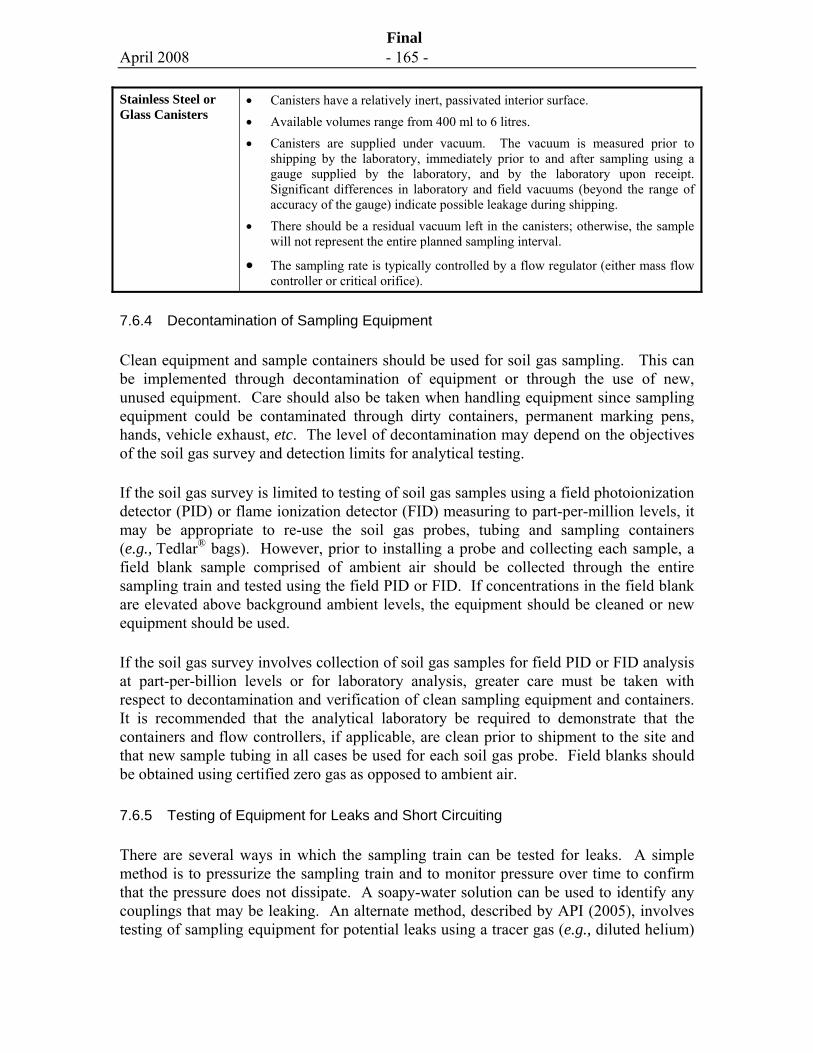
April 2008 - 165 -

Final

Stainless Steel or Glass Canisters

• Canisters have a relatively inert, passivated interior surface. • Available volumes range from 400 ml to 6 litres. • Canisters are supplied under vacuum. The vacuum is measured prior to

shipping by the laboratory, immediately prior to and after sampling using a gauge supplied by the laboratory, and by the laboratory upon receipt. Significant differences in laboratory and field vacuums (beyond the range of accuracy of the gauge) indicate possible leakage during shipping.

• There should be a residual vacuum left in the canisters; otherwise, the sample will not represent the entire planned sampling interval.

• The sampling rate is typically controlled by a flow regulator (either mass flow controller or critical orifice).

7.6.4 Decontamination of Sampling Equipment

Clean equipment and sample containers should be used for soil gas sampling. This can be implemented through decontamination of equipment or through the use of new, unused equipment. Care should also be taken when handling equipment since sampling equipment could be contaminated through dirty containers, permanent marking pens, hands, vehicle exhaust, etc. The level of decontamination may depend on the objectives of the soil gas survey and detection limits for analytical testing.

If the soil gas survey is limited to testing of soil gas samples using a field photoionization detector (PID) or flame ionization detector (FID) measuring to part-per-million levels, it may be appropriate to re-use the soil gas probes, tubing and sampling containers (e.g., Tedlar® bags). However, prior to installing a probe and collecting each sample, a field blank sample comprised of ambient air should be collected through the entire sampling train and tested using the field PID or FID. If concentrations in the field blank are elevated above background ambient levels, the equipment should be cleaned or new equipment should be used.

If the soil gas survey involves collection of soil gas samples for field PID or FID analysis at part-per-billion levels or for laboratory analysis, greater care must be taken with respect to decontamination and verification of clean sampling equipment and containers. It is recommended that the analytical laboratory be required to demonstrate that the containers and flow controllers, if applicable, are clean prior to shipment to the site and that new sample tubing in all cases be used for each soil gas probe. Field blanks should be obtained using certified zero gas as opposed to ambient air.

7.6.5 Testing of Equipment for Leaks and Short Circuiting

There are several ways in which the sampling train can be tested for leaks. A simple method is to pressurize the sampling train and to monitor pressure over time to confirm that the pressure does not dissipate. A soapy-water solution can be used to identify any couplings that may be leaking. An alternate method, described by API (2005), involves testing of sampling equipment for potential leaks using a tracer gas (e.g., diluted helium)

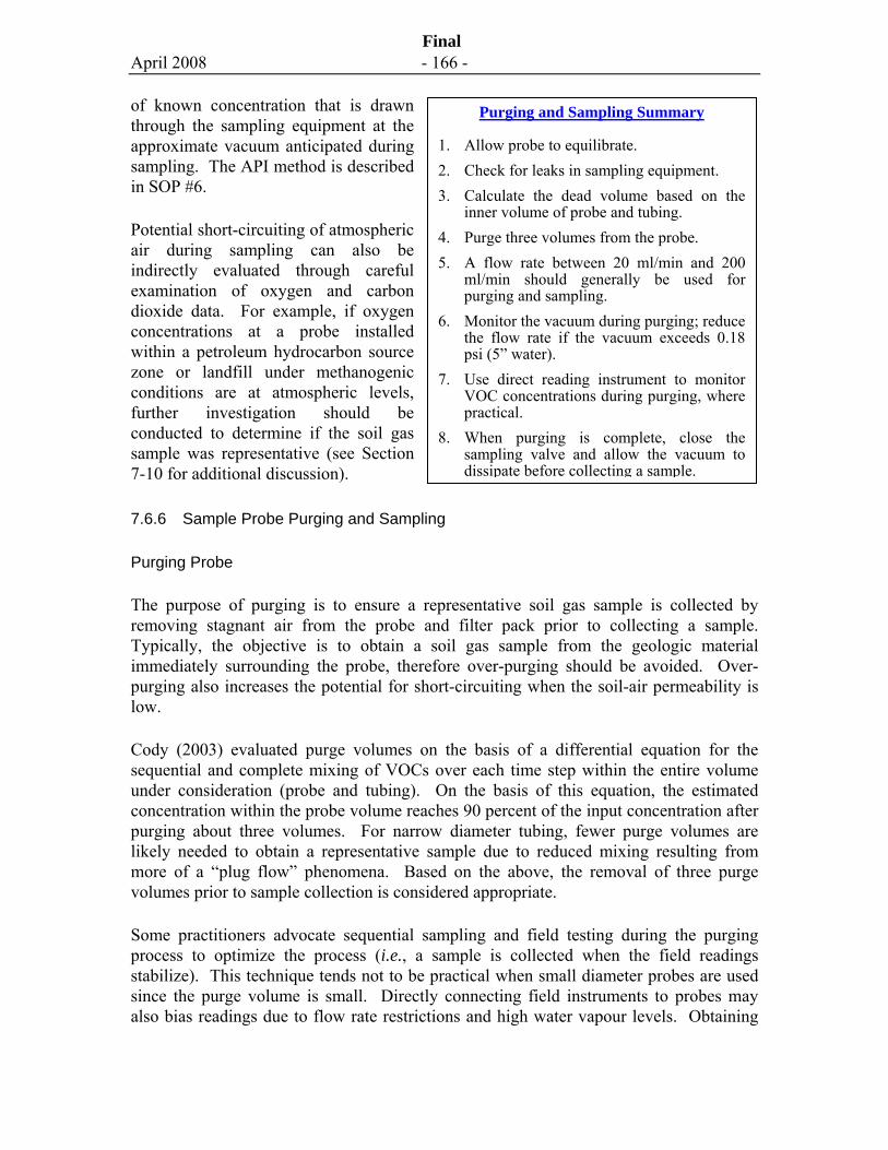
April 2008 - 166 -

Final

of known concentration that is drawn through the sampling equipment at the approximate vacuum anticipated during sampling. The API method is described in SOP #6.

Potential short-circuiting of atmospheric air during sampling can also be indirectly evaluated through careful examination of oxygen and carbon dioxide data. For example, if oxygen concentrations at a probe installed within a petroleum hydrocarbon source zone or landfill under methanogenic conditions are at atmospheric levels, further investigation should be conducted to determine if the soil gas sample was representative (see Section 7-10 for additional discussion).

7.6.6 Sample Probe Purging and Sampling

Purging Probe

The purpose of purging is to ensure a representative soil gas sample is collected by removing stagnant air from the probe and filter pack prior to collecting a sample. Typically, the objective is to obtain a soil gas sample from the geologic material immediately surrounding the probe, therefore over-purging should be avoided. Over-purging also increases the potential for short-circuiting when the soil-air permeability is low.

Cody (2003) evaluated purge volumes on the basis of a differential equation for the sequential and complete mixing of VOCs over each time step within the entire volume under consideration (probe and tubing). On the basis of this equation, the estimated concentration within the probe volume reaches 90 percent of the input concentration after purging about three volumes. For narrow diameter tubing, fewer purge volumes are likely needed to obtain a representative sample due to reduced mixing resulting from more of a “plug flow” phenomena. Based on the above, the removal of three purge volumes prior to sample collection is considered appropriate.

Some practitioners advocate sequential sampling and field testing during the purging process to optimize the process (i.e., a sample is collected when the field readings stabilize). This technique tends not to be practical when small diameter probes are used since the purge volume is small. Directly connecting field instruments to probes may also bias readings due to flow rate restrictions and high water vapour levels. Obtaining

Purging and Sampling Summary

1. Allow probe to equilibrate. 2. Check for leaks in sampling equipment. 3. Calculate the dead volume based on the

inner volume of probe and tubing. 4. Purge three volumes from the probe. 5. A flow rate between 20 ml/min and 200

ml/min should generally be used for purging and sampling.

6. Monitor the vacuum during purging; reduce the flow rate if the vacuum exceeds 0.18 psi (5” water).

7. Use direct reading instrument to monitor VOC concentrations during purging, where practical.

8. When purging is complete, close the sampling valve and allow the vacuum to dissipate before collecting a sample.

April 2008 - 167 -

Final

field readings during purging; however, may provide useful qualitative data for initial assessment of soil vapour conditions.

Larger Volume Purge Sampling

Larger purge volumes and longer sampling times may be desirable if the intent is to evaluate conditions beyond the immediate proximity of the soil gas probe. If the approximate permeability and soil gas flow regime is known, a volume-integrated concentration may be obtained. The concentration trends over time as measured by direct reading instruments may also provide qualitative information on spatial variability in source concentrations. For example, slowly increasing concentrations could indicate a higher soil gas concentration zone laterally removed from the probe. Large volume sampling may disturb the local equilibrium and therefore it may take some time for equilibrium conditions to be re-established.

Sampling Flow Rate

Recommended sampling flow rates range between about 1 L/hour and 1 L/minute (API, 2005). A sampling rate tied to the vacuum generated during sampling not exceeding 0.36 PSI (10” of water) (Lahvis, 2002) is also commonly referenced. The concern with higher flow rates and vacuums is the increased potential for leakage of air into the soil gas probes and probe tubing. High vacuums may enhance the volatilization of the more volatile compounds in a chemical mixture (API, 2005). For this guidance, a flow rate between 10 ml/min and 200 ml/min and a vacuum that is less than 0.18 PSI (5” of water) is recommended for soil gas purging and sampling. The vacuum can be easily measured using a T-junction connected to a digital manometer.

Sample Collection

Once purging is complete, soil gas samples from conventional soil gas probes should be collected using the same sampling flow rate as for purging. For subslab soil gas probes, it may be desirable to collect a subslab gas sample concurrently with an indoor air sample. Indoor air samples are typically obtained over a 24-hour period. The soil gas sampling rate for a 6-litre Summa sample collected over 24 hours is about 3.5 mL/minute to result in a residual vacuum of about 2.45 PSI (5” Hg). Sampling of probes at a site should be completed over a relatively short time period (e.g., within one week) to provide an internally consistent data set (Lahvis, 2002). If measurements with a portable multi-gas detector are to be made (e.g., oxygen, carbon dioxide), measurements should either be conducted well before (e.g., one day) the collection of the soil gas sample for laboratory analysis or after collecting the laboratory sample. If any water is drawn in the sample container, re-collect the sample after taking measures to eliminate water.

Sample Handling and Storage

Soil gas samples obtained using syringes, bags, canisters or cylinders should not be placed in a chilled cooler for transport since volatiles may condense out the vapour phase

April 2008 - 168 -

Final

at lower temperature (Hartman, 2002). Samples should not be subjected to excessive heat.

Tedlar® bags and glass cylinders should be placed inside a container immediately after collection to avoid possible photo-oxidation reactions.

For sorbent tubes, cool storage (approximately 4oC) in sealed containers is recommended. Sorbent tubes should be stored in a sealed plastic container containing a bed of activated carbon to minimize the potential for adsorption of ambient VOCs. All soil gas samples should be transported in separate containers from soil and groundwater samples.

7.7 Soil Gas Analysis

7.7.1 Selection of Method

Analytical testing methods appropriate for analyzing soil gas samples will be dependent on risk assessment objectives, sampling method and data quality objectives. Soil gas programs often consist of a combination of field testing of soil gas samples using hand-held detectors and laboratory analysis of selected soil gas samples for specific chemicals of potential concern. Since analytical testing is a broad topic, only an overview of the key issues is provided below. Common analytical methods for soil vapour are summarized in Table 7.4, with a detailed list provided in Appendix 7-1.

It is important to understand procedures and potential limitations associated with different testing methods. Since soil vapour and air methods are not as well defined as groundwater methods, adequate consultation with the laboratory is essential. The types of information that should be discussed include optimal sampling flow rate and duration, detection limits, laboratory QA/QC requirements and considerations, and the handling and transport of samples. Communication with the laboratory at the early stages ensures that important analytical considerations are taken into account during the development of the sampling plan.

7.7.2 Field Detectors

Field detectors commonly used are photoionization detectors (PID) or flame ionization detectors (FID), combustible gas detectors or explosimeters, and multi-gas detectors for compounds such as oxygen, carbon dioxide and methane, which are important for studies evaluating biodegradation. Photoionization detectors will respond to most organic vapours as well as some inorganic vapours (hydrogen sulphide, ammonia) depending on the ionization lamp energy. The sensitivity of a PID varies depending on the compound, and moisture can bias readings; therefore care should be taken when conducting soil gas surveys, particularly when connecting a PID directly to a soil gas probe. Combustible gas detectors are typically calibrated to methane in air, but also readily respond to heavier hydrocarbon (e.g., gasoline) vapours. Filters can be used to enable light (methane) and heavier organic vapours to be quantified, if desired. It is important to document the type

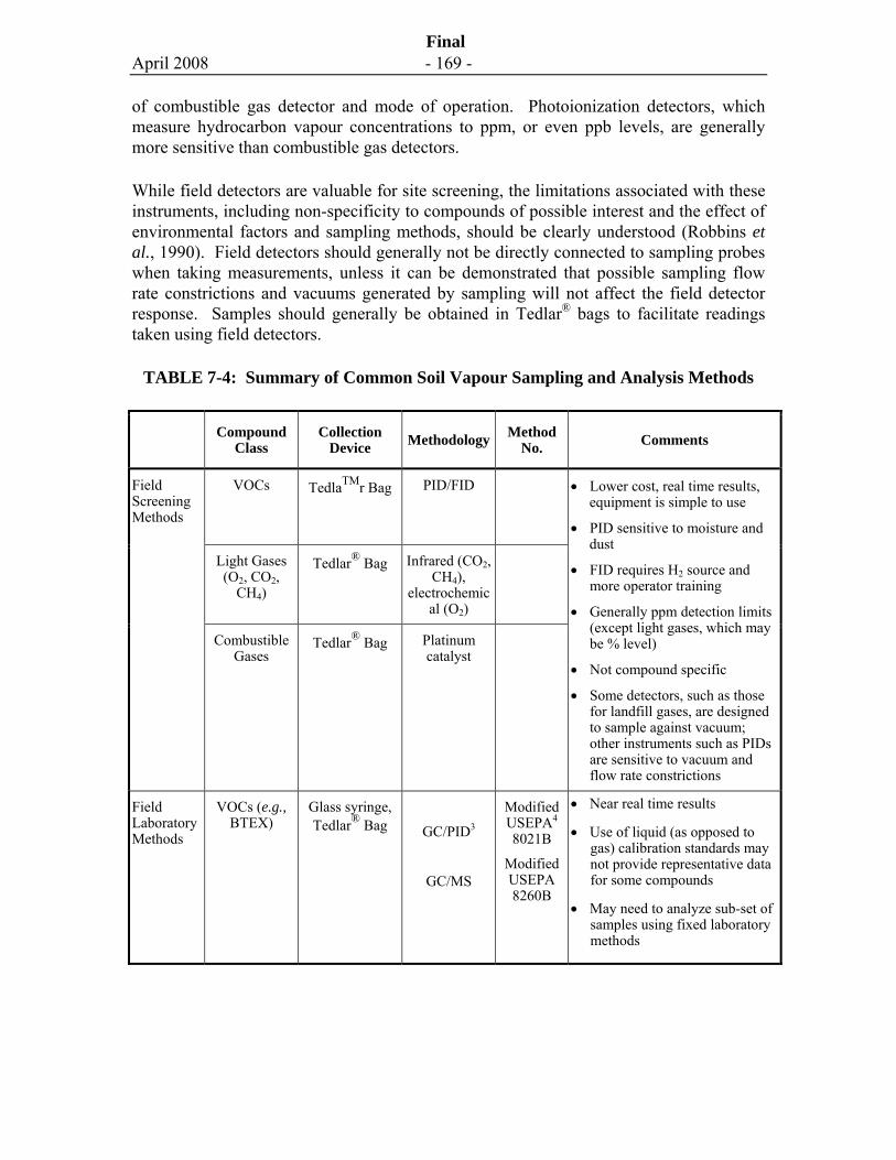
April 2008 - 169 -

Final

of combustible gas detector and mode of operation. Photoionization detectors, which measure hydrocarbon vapour concentrations to ppm, or even ppb levels, are generally more sensitive than combustible gas detectors.

While field detectors are valuable for site screening, the limitations associated with these instruments, including non-specificity to compounds of possible interest and the effect of environmental factors and sampling methods, should be clearly understood (Robbins et al., 1990). Field detectors should generally not be directly connected to sampling probes when taking measurements, unless it can be demonstrated that possible sampling flow rate constrictions and vacuums generated by sampling will not affect the field detector response. Samples should generally be obtained in Tedlar® bags to facilitate readings taken using field detectors.

TABLE 7-4: Summary of Common Soil Vapour Sampling and Analysis Methods

Compound Class

Collection Device Methodology Method

No. Comments

VOCs TedlaTMr Bag PID/FID

Light Gases (O2, CO2,

CH4)

Tedlar® Bag Infrared (CO2, CH4),

electrochemical (O2)

Field Screening Methods

Combustible Gases

Tedlar® Bag Platinum catalyst

• Lower cost, real time results, equipment is simple to use

• PID sensitive to moisture and dust

• FID requires H2 source and more operator training

• Generally ppm detection limits (except light gases, which may be % level)

• Not compound specific

• Some detectors, such as those for landfill gases, are designed to sample against vacuum; other instruments such as PIDs are sensitive to vacuum and flow rate constrictions

Field Laboratory Methods

VOCs (e.g., BTEX)

Glass syringe, Tedlar® Bag

GC/PID3

GC/MS

Modified USEPA4 8021B

Modified USEPA 8260B

• Near real time results

• Use of liquid (as opposed to gas) calibration standards may not provide representative data for some compounds

• May need to analyze sub-set of samples using fixed laboratory methods

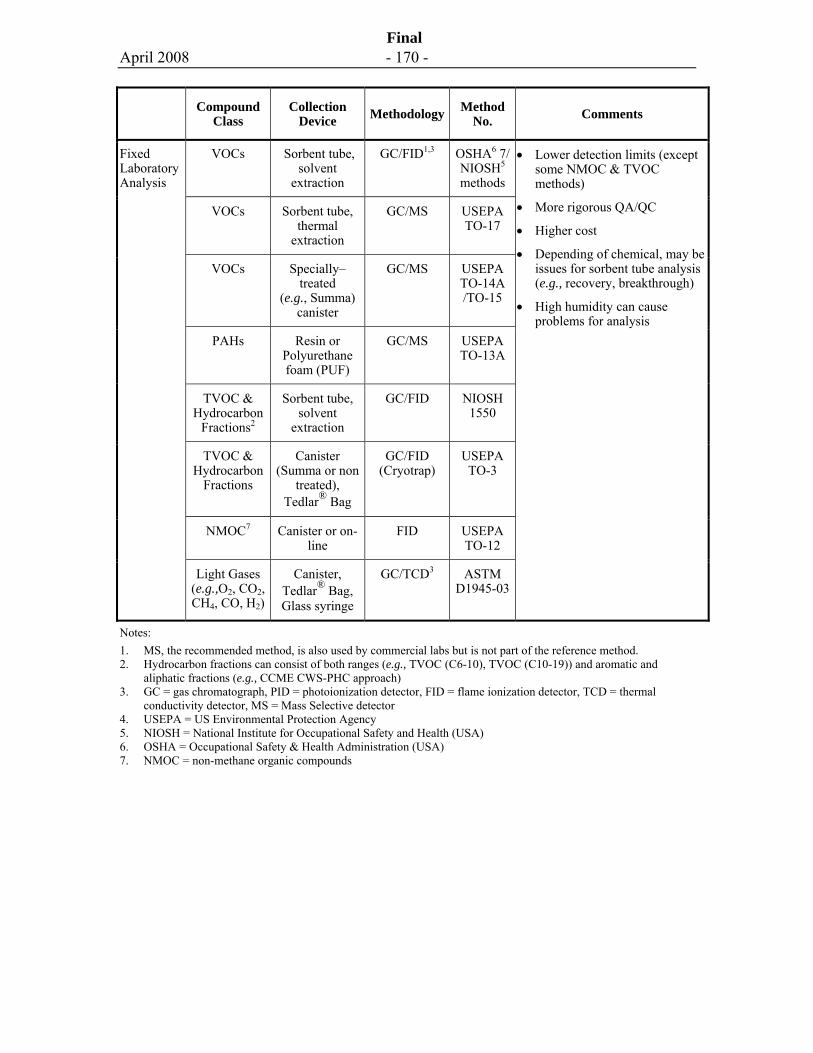
April 2008 - 170 -

Final

Compound Class

Collection Device Methodology Method

No. Comments

VOCs Sorbent tube, solvent

extraction

GC/FID1,3 OSHA6 7/ NIOSH5 methods

VOCs Sorbent tube, thermal

extraction

GC/MS USEPA TO-17

VOCs Specially–treated

(e.g., Summa) canister

GC/MS USEPA TO-14A /TO-15

PAHs Resin or Polyurethane foam (PUF)

GC/MS USEPA TO-13A

TVOC & Hydrocarbon

Fractions2

Sorbent tube, solvent

extraction

GC/FID NIOSH 1550

TVOC & Hydrocarbon

Fractions

Canister (Summa or non

treated), Tedlar® Bag

GC/FID (Cryotrap)

USEPA TO-3

NMOC7 Canister or on-line

FID USEPA TO-12

Fixed Laboratory Analysis

Light Gases (e.g.,O2, CO2, CH4, CO, H2)

Canister, Tedlar® Bag, Glass syringe

GC/TCD3 ASTM D1945-03

• Lower detection limits (except some NMOC & TVOC methods)

• More rigorous QA/QC

• Higher cost

• Depending of chemical, may be issues for sorbent tube analysis (e.g., recovery, breakthrough)

• High humidity can cause problems for analysis

Notes: 1. MS, the recommended method, is also used by commercial labs but is not part of the reference method. 2. Hydrocarbon fractions can consist of both ranges (e.g., TVOC (C6-10), TVOC (C10-19)) and aromatic and

aliphatic fractions (e.g., CCME CWS-PHC approach) 3. GC = gas chromatograph, PID = photoionization detector, FID = flame ionization detector, TCD = thermal

conductivity detector, MS = Mass Selective detector 4. USEPA = US Environmental Protection Agency 5. NIOSH = National Institute for Occupational Safety and Health (USA) 6. OSHA = Occupational Safety & Health Administration (USA) 7. NMOC = non-methane organic compounds

April 2008 - 171 -

Final

7.7.3 Field Laboratory Analysis

Field laboratory methods are used when a greater degree of precision or component-specific information is required than that provided by a field screening method. The advantage of field laboratory methods are near real-time results, which can be used to modify programs while in progress, and potentially lower costs. Also the ability to collect repeat samples can be an advantage for assessing sampling, temporal, and spatial variability. The disadvantage of field laboratory methods are higher detection limits than fixed laboratory methods based on USEPA TO- protocols (see below). Possible regulatory requirements for soil gas analytical protocols should also be reviewed when evaluating field laboratory analysis.

Field laboratory methods include the use of portable gas chromatographs (GCs) that are brought to the site to analyze grab samples on an on-going basis. Soil gas air is usually collected using gas-tight syringes and is injected into the GC (or purge-and-trap apparatus) for analysis. The portable GC usually analyses data through photo ionization, flame ionization or electron capture detectors (e.g., modified USEPA Method 8021B). The precision of the results can vary depending on the equipment used. Portable mass spectrometers (MS) are also being introduced to the market, which provide greater certainty for compound identification (e.g., modified USEPA Method 8260B). Modified water methods (USEPA Method 8021B and 8260B) can work well for many compounds, but for non-polar compounds and heavier molecular weight compounds such as naphthalene, recovery tends to be poor (Hayes et al., 2005).

7.7.4 Fixed Laboratory Analysis

For risk assessment studies, low detection limits and more rigorous quality control requirements typically require that soil gas samples be collected using either active sorbent tubes (i.e., air is drawn through tube using pump) or steel canisters, and quantified by GC/MS methods at fixed laboratory locations. The use of GC/FID analysis is generally not recommended due to non-specificity of detection but may be used in the assessment of CCME F1 and F2 criteria for certain test methods (Appendix 7-2).

Sampling using a sorbent tube is an indirect method of estimating the soil vapour concentration in that the test measures the mass of chemical trapped on the sorbent. The air concentration is estimated by dividing the mass by the total volume of air drawn through the tube. The canister method involves collection of a “whole air” sample enabling direct analysis of the soil vapour sample. Both methods are described in detail below.

April 2008 - 172 -

Final

Selection of Method

The chemical to be measured, detection limit, ease of use, cost, laboratory certification and quality control are factors that should be considered when selecting the soil gas analysis method. Sorbent tubes analyzed by modified OSHA or NIOSH methods may be used to measure a wide range of VOCs to detection limits typically required for soil vapour; however, breakthrough for light molecular weight VOCs (e.g., vinyl chloride) can be difficult to control. Summa canisters can be used to measure a wide range of VOCs including naphthalene. Analysis by GC/MS is recommended regardless of the collection method, except when hydrocarbon fractions are analyzed (see Appendix 7-2). Tedlar® bags should not be used to collect samples for VOC analyses, with exception of light gas analyses (e.g., ASTM D1945-03) where the method specifically calls for bags to be used. Sorbent Tube Method

The use of sorbent tubes for sampling and analysis of soil vapour is relatively complicated and there are numerous factors to consider. While a number of methods are available, it is important to recognize that they are air methods that have been modified for soil vapour.

Analytical Methods: A key distinguishing factor between methods is whether thermal desorption (e.g., USEPA TO-17) or solvent extraction is used (e.g., modified OSHA 7 or NIOSH 1501 methods).

Thermal desorption involves rapidly heating the sorbent to desorb the VOC, while passing an inert carrier gas through the tube. The VOCs are carried by the gas and concentrated on a smaller downstream trap, which usually is cryogenically cooled. For thermal desorption, the whole sample is released from the sorbent during the heated desorption step. While some of the earlier thermal desorption units do not allow for the possibility for replicate analyses, the newest units have the capability of re-collecting a portion of sample during the primary desorption step to allow for re-analysis. Additionally, sample introduction parameters can be modified such that less mass is loaded onto the GC/MS in order to perform sample dilutions (this is important since soil vapour concentrations, as compared to air, can be very high and potentially overload the GC/MS). The sensitivity of thermal desorption techniques requires a smaller soil gas volume to meet screening levels than solvent extraction techniques.

Solvent extraction involves use of a solvent such as carbon disulphide to extract the sample. In contrast to thermal desorption, replicate analyses can be performed on the extract. While chemical extraction methods are adapted from industrial hygiene practice and are typically not as sensitive as thermal desorption, higher detection limits may not be an issue for soil vapour analysis (but may be problematic for air analyses). To achieve low detection limits, NIOSH or OSHA methods involving chemical extraction are modified and typically utilize a larger mass of sorbent combined with longer sampling

April 2008 - 173 -

Final

durations. As discussed below, longer sampling durations can pose challenges in terms of breakthrough.

Types of Sorbents: Sorbents used for VOCs commonly used consist of charcoal, polymeric and/or carbonaceous resins. There are wide variations in sorbent properties. Since soil gas typically has a relative humidity of close to 100 percent, hydrophobic sorbents are preferred since sorbed water reduces the retention of VOCs, and because water vapour can affect the GC analysis (Harper, 1994). Polar VOC compounds can also partition into the water phase reducing recovery. Elevated ozone levels (150 ppm to 300 ppm) have been reported to result in reduced recovery for certain VOCs such as styrene and aldehydes (McClenny et al., 2002). Other issues for sorbent sampling include sorbent pore size and uniformity, possible reactions between the sorbent and adsorbed molecules, and slow breakdown of certain polymeric sorbents and release of aromatic hydrocarbons (Harper, 1994). Special attention should be paid to sorbents selected for analysis of highly volatile chemicals such as vinyl chloride, which are difficult to trap using sorbent media.

The laboratory methods typically specify the type of sorbent to use. Coconut shell charcoal is typically used for BTEX analysis (NIOSH 1501). For chlorinated solvent compounds, some laboratories use the same method but substitute newer more sorptive materials such as processed synthetic carbon (e.g., Anasorb 747) or molecular sieve materials in place of the coconut shell charcoal. For USEPA TO-17 analysis, combining hydrophobic sorbents of increasing strength allows the collection of a wider volatility range. For example, sorbent tubes containing a combination of Tenax, Carbograph 1TD, and Carbograph 5 TD were shown to successfully retain lighter VOCs such MTBE while allowing for the efficient desorption of naphthalene under sample conditions of high humidity (Hayes et al., 2007). Sorbents exhibiting water retention should be used with extreme caution as the water adsorbed from soil gas collection can result in problems during sample analysis. Hayes et al. (2007) showed that water adsorption on a multi-bed sorbent tube containing Carbosieve S-III resulted in analytical interference resulting in unuseable data. These effects were noted under conditions of approximately 75% relative humidity and sample volumes as low as 2 liters. Sorbents used for semi-volatile (PAH) analyses (naphthalene and heavier molecular weight compounds) often consist of Teflon®-impregnated glass fibres followed by a resin (XAD-2) sorbent (NIOSH 5515 or USEPA Method TO-13A). Since trapping of particulates for soil vapour is usually not an objective, typically only the XAD resin sorbent is used for semi-volatile analyses (i.e., polyurethane (PUF) foam is not used).

Sorbent Sampling Volume: The sampling volume should be carefully determined through consideration of the expected VOC concentration and mass, the sorption capacity and required detection limits. When available, the results of field PID analyses of soil vapour should be communicated to the laboratory analyst prior to sorbent sampling to guide selection of a sampling

Sampling Volume Calculation

An example sampling volume calculation is provided for sorbent tube analysis for benzene. Assuming a target indoor air concentration of 3 μg/m3, a target detection limit of 30 μg/m3 is obtained (Eq. 7-1 Section 7.7.5). A typical benzene detection limit is 0.1 μg (MS detector), therefore approximately 3.3 litres of soil gas would need to be drawn through the tube (0.1μg/30μg/m3 X 1000 L/m3). At a sampling rate of 100 ml/min, the required sampling duration would be 33 minutes.

April 2008 - 174 -

Final

duration and flow rate that would minimize the potential for chemical breakthrough. An option is to collect two samples over different time durations to avoid the possibility of re-sampling.

Pump Flow Rate: Since the concentration is sensitive to the flow rate, pumps must be accurately calibrated and provide a constant flow rate throughout the sampling duration. The pump flow rate must be checked prior to and during sampling, since actual pump flow rates may vary considerably depending on the soil air permeability and vacuum. A recent study (Golder Associates, 2007, unpublished) found a significant and roughly linear drop in pump flow rate under vacuum conditions induced by soil (e.g., 11% drop in flow at 3.4 inches H20, 40% drop at 9 inches H20 and 93% drop at 16.5 inches H20).

Environmental Conditions: Appropriate measures should be taken to mitigate the effects of high humidity or cold weather when sampling using sorbent tubes, which may not always be practical to avoid. Reducing the air flow rate or sampling with varying volumes of air (using multiple samples) may be a good approach under this circumstance. Further discussion on cold weather considerations is provided in Exhibit 7-1.

Canister Method

Low detection limits can be achieved utilizing canister samples testing in accordance with USEPA Method TO-15 and, in general, the accuracy and precision of analytical results generated are high. Nevertheless, there are significant issues for this method as described below.

Analytical Methods: The analytical protocols for the Summa method are USEPA TO-14A (non-polar compounds) (USEPA, 1999a) and USEPA TO-15 (polar and non-polar compounds) (USEPA, 1999b). USEPA Method TO-15 is commonly used for soil vapour analyses since there are a number of significant improvements for Method TO-15 compared to TO-14A, including enhanced measures for quality control (e.g., 5-point calibration), specific canister cleaning procedures, better water management procedures and better recovery of polar compounds. USEPA Method TO-15 utilizes a gas chromatograph (GC) with a mass spectrometer (MS) as the detector. When the MS is run in full scan mode up to 70 compounds can be readily detected with typical reporting limits between 0.2 to 0.5 parts per billion by volume (ppbV). Analytical methodology considerations are further discussed in Section 8.4.1.

Hardware: Two types of canisters are available: Summa canisters, which are electro-polished steel canisters and Silco canisters, where the steel is coated with an inert fused silica layer.3 It is important that the canister hardware be in good condition. For soil vapour sampling, a one-litre canister is typically a sufficient volume.

3 The silcosteel canisters internal surface is intended to be non-reactive with sulphur compounds or compounds that react with metal surfaces (e.g., polar compounds). However, there is debate between practitioners on appropriate sampling device for sulphur compounds, with some advocating the use of Tedlar® bags.

April 2008 - 175 -

Final

The flow regulator (mass flow controller or critical orifice) should be appropriately calibrated based on the desired sampling duration and the vacuum before sampling and residual vacuum after sampling should be recorded. Flow regulators are temperature and altitude dependent; therefore, the sampling location should be communicated to the laboratory so that appropriate adjustments can be made.4 A critical orifice is often used for short duration sampling for soil vapour (i.e., up to an hour), but it does not provide for an uniform flow since the flow rate is a function of the pressure differential. This is not of significant concern for soil vapour sampling; however, a residual vacuum should remain in the canister after sampling is complete. For longer duration sampling (e.g., indoor air sampling), a mass flow controller should be used to provide for an uniform flow rate. Particulate filters consisting of sintered steel with 2 to 7 micron pore sizes or deactivated glass frit are placed before the critical orifice. It is essential that all fittings are tight during sampling.

Equipment Cleaning: The TO methods and hardware were designed to measure low VOC concentrations in ambient air. At some sites (e.g., dry cleaners, UST sites with free-phase NAPL), canisters are subject to soil vapour concentrations that exceed 100,000 to 1,000,000 ug/m3. Experience has shown that there is a significant potential for contaminant carry over in the canister, regulator, filter or inlet tube under these conditions. Therefore, all equipment must be thoroughly cleaned and canister blanks tested. Canisters are typically cleaned by the laboratories by heating the canister and passing humidified zero air under pressure through the canister.

For heavier molecular weight compounds (trimethylbenzene and heavier), sorption onto metal tubing and filter has been shown to result in reduced compound recovery (Entech, 2007).

Environmental Conditions: For Summa canisters, some water vapour is needed to coat the inside of the surface of the steel to provide for an inert surface. However, similar to sorbent tubes, excessive water can create challenges for sample recovery and cryogenic focusing prior to analysis, although an alternate method of multiple focusing steps using non-cooled sorbent tubes can reduce problems associated with water vapour.

Note the barometric pressure at both sampling and laboratory location. When there are significant differences in the elevation at which the sample was obtained and the laboratory, it may be possible to correct for the effect of ambient barometric pressure on the sample concentration (i.e., using Boyle’s Law for an ideal gas).

4 Laboratories typically conduct performance studies to verify that flow regulator’s provide for an uniform sampling rate over the sampling duration, within an acceptable tolerance. If warranted, flow rates can be verified in the field using an extra canister using an electronic mass flow meter or rotometer, calibrated for vacuum conditions.

April 2008 - 176 -

Final

7.7.5 Quality Assurance / Quality Control Considerations

Data Quality Objectives

Data quality objectives should be established as part of the sampling plan in conjunction with the overall study objectives. In broad terms, the data quality objective is to ensure that data quality is acceptable and that data can be relied upon for decision-making purposes. Specific objectives may be developed in terms of accuracy, precision, data representativeness, data completeness and detection limits. There may also be specific considerations for cold weather sampling that should be incorporated in the data quality objectives (Exhibit 7-1).

The development of a QA/QC plan will help to ensure that the desired data quality is achieved. Standard operating procedures should be used for sampling and analytical

Exhibit 7-1: Considerations for Cold Weather Sampling

In many regions of Canada, environmental investigations may be completed during periods of relatively cold weather (i.e., freezing temperatures). For soil vapour sampling design the influence of frost and snow cover on the soil vapour transport should be considered. Frost and snow cover may limit the flux of contaminant vapours to atmosphere and oxygen recharge to subsurface. There may also be significant temperature gradients between shallow soil beside and below a building, where the temperature may be well above freezing. Obtaining a soil vapour sample within frozen ground, while potentially feasible, is not considered representative and therefore either deeper external vapour samples or samples from below the building should be obtained.

Certain pre-cautions should also be taken when conducting soil vapour programs during cold weather. Field instruments such as photoionization and flame ionization detectors and pumps are not designed to operate when temperatures are below freezing. Field instruments may be kept warm in a heated building or vehicle, with field samples collected and transported in Tedlar® bags. Sampling pumps may be kept warm by storing them in insulated coolers or insulated lunch bags with heat packs. Condensation may occur through cooling of warmer soil gas during sampling. Condensation can be particularly problematic for sorbent tube sampling and therefore sample tubing and bags should be closely observed for any signs of condensation (e.g., through use of translucent tubing). During cold weather, sorbents and tubing should be heated and insulated to minimize condensation and prevent freezing; however, tubes should not be over-heated since sorption efficiency decreases with increasing temperature. Tubing should be kept as short as possible.

April 2008 - 177 -

Final

procedures, including the use of chain-of-custody records and identifying sampling locations. Systematic data collection and planning helps provide for defensible results and increased credibility.

Detection Limits

For risk assessments, the measured vapour concentrations are often used to predict indoor air concentrations. Required detection limits can be back-calculated using risk-based target indoor air concentrations combined with minimum expected dilution factors between soil vapour and indoor air. A lower bound dilution factor for the soil vapour to indoor air transport pathway of 100 may be used to estimate the required detection limit. An additional adjustment factor (about 5 to 10X, where possible) should be applied to provide for greater flexibility in data interpretation and since there is increased uncertainty near to the detection limit. The maximum detection limit is calculated as follows:

DLmax = DF * Cair / AF [7-1]

Where DL is the analytical reporting (detection) limit, DF is the dilution factor (100), Cair is the target indoor air concentration, and AF is adjustment factor (5 to 10).

Testing and Certification that Sampling Device is Clean

For all methods, it is recommended the analytical laboratory demonstrate that the sampling device (canister, sorbent tube) is clean to below the required detection limits prior to sampling and analysis, for either a representative subset or all of the sampling devices. Depending on the project requirements, either batch or individual certification of the sampling device may be warranted.

Quality Control Samples

Analysis of duplicate samples is required to assess the precision of the method and variability of the sampling process. The field duplicate samples should be obtained from the same soil gas probe using identical sampling procedures and submitted blind to the laboratory. Duplicate samples can either be obtained simultaneously (i.e., using a splitter) or in sequence. When duplicate samples are collected in sequence, variability due to temporal changes is introduced. For indoor and ambient air sampling, a duplicate sample may be obtained using a splitter or side-by-side (collocated) samples may be obtained.

The frequency of field and laboratory duplicate sample analyses, while often each set at 10 percent of the samples analyzed, may depend on the total number of samples analyzed and analytical method. When only a small number of samples are tested, it may be

April 2008 - 178 -

Final

desirable to increase the frequency of testing or pool QC results from multiple programs before drawing conclusions about data quality. Depending on whether the laboratory has a thermal desorption unit with re-collection feature, collection of duplicate samples for thermal desorption analyses may be advantageous in that it enables re-analysis of a second sample.

While not a duplicate analysis, for sorbent tube analysis, both the front and back sections of sampling tubes (or two tubes in series) should be analyzed separately to evaluate for chemical breakthrough.

Depending on project requirements, other quality control samples that may be analyzed include transport blanks, method blanks and spike samples, as described below:

• Field transport blanks are sample containers that are shipped with the other samples, but which are not used for collecting a sample. For Summa canisters, testing a field transport blank involves filling the canister with ultra high purity air or nitrogen, which should be supplied by the laboratory in a separate canister.5

• A field method blank may be collected by drawing atmospheric air or high purity inert gas through the sampling train and probe to be sampled, prior to installation. This can provide useful data on whether the sampling train is clean.

• Sample tubes spiked with known concentrations of analytes are used to evaluate the recovery of the spiked compound and accuracy of the extraction and analytical procedure. This type of test is normally performed by the analytical laboratory.

All data should be clearly reported, including blanks, and any suspect results should be flagged. The interpretation of quality control data is discussed in Section 7.10.

7.8 Soil and Groundwater Characterization

It is often preferable to evaluate the soil vapour intrusion pathway using directly measured soil vapour concentrations. However, soil and/or groundwater data are critical for developing the CSM that is used to guide the development of the soil vapour characterization program. Soil data can be used to evaluate contamination source zones, including possible sources that are located above the water table. Shallow groundwater data and predictions of deep soil vapour concentrations along with measured deep vapour concentrations can be used to evaluate the degree to which volatilization from groundwater and migration through the capillary fringe occurs, or the degree to which it may be inhibited through infiltration or geologic barriers. In some cases, it may not be possible to collect a representative soil gas sample due to low permeability deposits;

5 For Summa canisters, a field transport (“trip”) blank provides limited information on potentially cross contamination during shipment and handling, but does provide for another check on cleaning of canisters.

April 2008 - 179 -

Final

therefore, the use of soil and/or groundwater data alone may be required for evaluation of the soil vapour intrusion pathway.

7.8.1 Groundwater Data

Groundwater characterization for evaluation of soil vapour intrusion should provide information on concentrations in groundwater near to the water table. This is because cross-media transfer from groundwater to soil vapour occurs when chemicals in pore-water volatilize into soil gas, which occurs in the capillary transition zone above the water table. Since there can be significant vertical concentration stratification, the use of relatively short monitoring well screens situated across the water table or depth discrete sampling methods such as the GeoprobeTM, Waterloo ProfilerTM or HydropunchTM methods are recommended when evaluating the soil vapour intrusion pathway.6 Depth discrete samples can also be obtained from existing monitoring wells using Passive Diffusive Bag Samplers (Vroblesky and Hyde, 1997; ITRC, 2002). Diffusive Bag Samplers can also be used to measure VOC concentrations in pore-water within the capillary transition zone.

As well screen lengths increase, there is increased blending of groundwater across the screened interval. This may result in either over-estimation or under-estimation of concentrations at the top of the aquifer, depending on the contamination scenario. At locations where LNAPL is present or where there is an interface plume from fluctuating water table and interaction between soil gas and the water table, longer well screens may under predict concentrations near the top of the aquifer. Where there is a fresh-water lens or contamination source below the water table (e.g., DNAPL), longer well screens may over predict concentrations near the top of the aquifer.

Groundwater well installation, well development and purging prior to sampling should be conducted according to current standards of practice. For vapour intrusion assessments, a saturated screen length of 1 to 2 m is recommended. Low flow purging and sampling methods that minimize disturbance, aeration and/or de-gassing of groundwater are recommended (Puls and Barcelona, 1996). Particular attention should be given to groundwater samples collected from submerged screens or wells with long screen intervals. The concentrations from these wells may be of limited value for vapour intrusion assessments.

While the appropriate focus of groundwater investigations for vapour intrusion studies is shallow groundwater quality, in some cases, it may also be important to assess the deeper groundwater quality. This is because contaminants at depth within groundwater systems could pose future vapour intrusion potential for hydrogeologic systems that undergo changes, due to natural seasonal fluctuations of the water table elevation and/or through human activities. The vertical concentration variability can be investigated either through

6 Another potential option may be to install small diameter implants (e.g., 15 cm long) at several depths near the water

table, which can be used to sample either soil gas or groundwater depending on water table fluctuations.

April 2008 - 180 -

Final

the use of nested wells (at different elevations) or vertical profiling using a Geoprobe or similar groundwater sampling technique as discussed in Section 6.0 of this document.

While in general, shallow groundwater quality data should be used for vapour intrusion assessment, deeper data should be used if deeper groundwater concentrations are higher than shallow concentrations and where potential future changes to groundwater systems could result in shallow data being non-representative.

7.8.2 Soil Data

There are a number of uncertainties associated with use of soil data for evaluation of soil vapour intrusion as a result of losses of volatile contaminants during soil sampling, handling and chemical analysis. Depending on the contaminant type and geologic conditions, there may be significant spatial variation in soil concentrations, which may be difficult to detect based on conventional sampling programs. Finally, there are uncertainties associated with soil partitioning calculations and predicted soil vapour concentrations are sensitive to the partitioning coefficient between water and organic carbon, and the fraction organic content in soil, a parameter that can be difficult to accurately determine. If soil analyses results are to be used for the vapour pathway, it is recommended that the soil samples be field preserved (e.g., using methanol), where possible (e.g., USEPA SW-846 Method 3035). A multi-functional sampling device (MFSDs), which act as a coring tool and airtight storage container, can also be used to collect soil samples for volatile analysis (e.g., EnCore™ Sampler). The storage chamber is completely soil filled with zero headspace and is then capped to form an airtight seal.

7.9 Ancillary Data

In addition to measured soil vapour concentrations, the supplemental data below may assist in understanding the vapour intrusion pathway. This information may have been collected as part of an environmental site assessment. However, supplementary data collection may be required if sufficient information was not collected during investigations completed prior to the soil vapour sampling program.

Physical Properties: The properties of soil layers of the vadose zone, including soil moisture, bulk density, air- and water-filled porosity and total organic carbon content may be important in evaluating vapour intrusion. Care should be taken to minimize re-distribution of soil moisture or drying of soil during drilling, sampling and storage of samples. Water retention tests on samples compacted to approximate in situ density can provide useful data on the likely range of water-filled porosity that could be expected in soil. Although not commonly performed, consideration can also be given to in situ tests to provide estimates of tortuosity (effective diffusion coefficient) (Johnson et al., 1998; Lahvis et al., 1999) and soil-air permeability (Baehr et al., 1991).

Hydrogeological Properties: The groundwater elevation during sampling and during an appropriate period prior to sampling is important when evaluating the possible seasonal

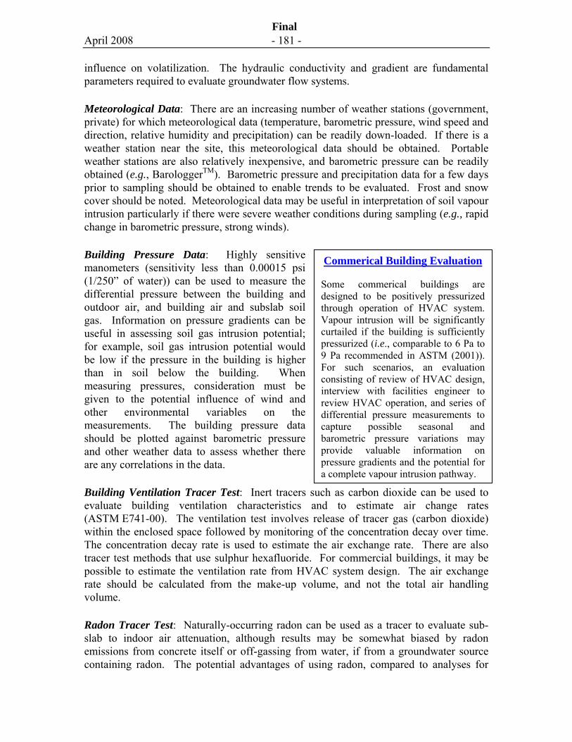
April 2008 - 181 -

Final

influence on volatilization. The hydraulic conductivity and gradient are fundamental parameters required to evaluate groundwater flow systems.

Meteorological Data: There are an increasing number of weather stations (government, private) for which meteorological data (temperature, barometric pressure, wind speed and direction, relative humidity and precipitation) can be readily down-loaded. If there is a weather station near the site, this meteorological data should be obtained. Portable weather stations are also relatively inexpensive, and barometric pressure can be readily obtained (e.g., BarologgerTM). Barometric pressure and precipitation data for a few days prior to sampling should be obtained to enable trends to be evaluated. Frost and snow cover should be noted. Meteorological data may be useful in interpretation of soil vapour intrusion particularly if there were severe weather conditions during sampling (e.g., rapid change in barometric pressure, strong winds).

Building Pressure Data: Highly sensitive manometers (sensitivity less than 0.00015 psi (1/250” of water)) can be used to measure the differential pressure between the building and outdoor air, and building air and subslab soil gas. Information on pressure gradients can be useful in assessing soil gas intrusion potential; for example, soil gas intrusion potential would be low if the pressure in the building is higher than in soil below the building. When measuring pressures, consideration must be given to the potential influence of wind and other environmental variables on the measurements. The building pressure data should be plotted against barometric pressure and other weather data to assess whether there are any correlations in the data.

Building Ventilation Tracer Test: Inert tracers such as carbon dioxide can be used to evaluate building ventilation characteristics and to estimate air change rates (ASTM E741-00). The ventilation test involves release of tracer gas (carbon dioxide) within the enclosed space followed by monitoring of the concentration decay over time. The concentration decay rate is used to estimate the air exchange rate. There are also tracer test methods that use sulphur hexafluoride. For commercial buildings, it may be possible to estimate the ventilation rate from HVAC system design. The air exchange rate should be calculated from the make-up volume, and not the total air handling volume.

Radon Tracer Test: Naturally-occurring radon can be used as a tracer to evaluate sub-slab to indoor air attenuation, although results may be somewhat biased by radon emissions from concrete itself or off-gassing from water, if from a groundwater source containing radon. The potential advantages of using radon, compared to analyses for

Commerical Building Evaluation

Some commerical buildings are designed to be positively pressurized through operation of HVAC system. Vapour intrusion will be significantly curtailed if the building is sufficiently pressurized (i.e., comparable to 6 Pa to 9 Pa recommended in ASTM (2001)). For such scenarios, an evaluation consisting of review of HVAC design, interview with facilities engineer to review HVAC operation, and series of differential pressure measurements to capture possible seasonal and barometric pressure variations may provide valuable information on pressure gradients and the potential for a complete vapour intrusion pathway.

April 2008 - 182 -

Final

VOCs, are potentially lower analytical costs, there are no common sources of indoor radon, and less bias is caused by non-detect values.

Passive Soil Vapour Samplers: Passive diffusion samplers contain a hydrophobic adsorbent material that collects organic compounds over time. The adsorbed compounds are removed from the adsorbent by thermal desorption or solvent extraction, and typically analyzed using GC/MS methods. The passive soil gas method provides the mass of vapours adsorbed to the media, but currently can not reliably be used to estimate soil vapour concentrations. Passive soil gas samples are typically deployed for a few days to weeks, and therefore provide a time-integrated sample. The extended sampling duration also provides for high sensitivity. In the context of soil vapour intrusion studies, passive soil gas sampling methods could be useful in mapping the location of subsurface plumes and for identifying pathways (in particular when placed in or along utility corridors) for determining locations for permanent probe placement when the CSM is not well understood.

Passive diffusive samples can be used to estimate VOC concentrations in air and are described in Chapter 8.

7.10 Data Interpretation and Analysis

The procedures for data interpretation and analysis of soil vapour data are described below. A detailed checklist for persons reviewing soil vapour assessment reports is provided in Volume 2.

7.10.1 Data Organization and Reporting

The soil gas data should be tabulated and plotted to facilitate evaluation and review of data relationships and trends. The following data organization and presentation is recommended:

• Tabulate all data including sample location identifier, sample date, sample depth, sampling methods (including sampling duration and flow rate), chemical analysis methods, laboratory detection limits and results of chemical analysis;

• Tabulate field screening and laboratory analysis data to enable side-by-side comparisons;

• Prepare plan drawings showing soil vapour concentration data that includes pertinent structures (buildings, utilities, paved areas, vegetated areas);

• Compare soil vapour with nearby groundwater concentration data; consider geologic conditions when evaluating variability;

• Prepare vertical profiles of soil vapour concentration data that includes oxygen, carbon dioxide and methane and boring log data where available; and,

April 2008 - 183 -

Final

• Identify soil vapour target concentrations and background indoor and outdoor air concentrations, where available.

7.10.2 Data Quality Analysis

Following receipt of the soil vapour results, the data should be evaluated to determine whether they meet data quality objectives outlined in the sampling plan (Section 7.7.5 and Chapter 3). The data quality checks should include the following:

• Review reported detection limits relative to data quality objectives. In some cases, sample dilution is required, which results in raised detection limits.

• For Summa canister analyses, review canister pressure upon completion of sampling and receipt by the laboratory. There should be a small vacuum left in the canister, if not, the sample integrity could be compromised. Obtain pre-delivery canister testing and certification results from the laboratory. Note and correct for the effect of ambient barometric pressure differences between the laboratory and sampling location on the sample concentration, as appropriate.

• For sorbent tube analyses, review results of analyses of front and back sections of the tube (or two tubes in series) to evaluate possible chemical breakthrough. Breakthrough can be caused when the adsorptive capacity is exceeded, the air flow through the tube is too high, and chromatographic effects caused by other compounds. If the laboratory considers the first tube saturated, then results are potentially biased and re-sampling should occur. The criterion for evaluating breakthrough is method and chemical dependent but typically is a concentration in the second tube that is greater than 10 to 25 percent of the concentration in the first tube. If the sample media is not saturated, the front and back concentrations should be added together for numerical evaluation.

• Compare precision for laboratory and field duplicate or co-located samples, as quantified by relative percent difference (RPD). The acceptable precision is method and chemical dependent, but for laboratory duplicates is generally 20 percent. For field duplicates, the acceptable RPD is higher since there is sampling variability in addition to laboratory variability.

• Review analytical results for blank samples (e.g., field blanks, laboratory blanks and trip blanks) to identify possible issues with the laboratory or field procedures that may have affected the results.

• Recognize that reported concentrations within five times of the quantification limit are typically more uncertain than higher concentration values.

April 2008 - 184 -

Final

7.10.3 Data Consistency Analysis

The results of the soil gas sampling program should be reviewed in terms of the expected results, based on consistency with the conceptual site model and internal consistency between sampling points. These consistency checks should include the following:

• The soil vapour concentrations should be spatially consistent with the soil and groundwater concentrations, for example, the highest soil vapour concentration should be measured in source contamination areas where soil and groundwater concentrations are also highest.

• The soil vapour concentrations should decrease with increasing distance from a source, and, in general for petroleum hydrocarbon sources, oxygen concentrations should decrease and carbon dioxide concentrations should increase close to petroleum hydrocarbon sources. If this pattern is not observed, there may be additional contamination sources present or there may be data quality issues (e.g., short circuiting).

• The vertical gradients of petroleum hydrocarbon vapours, oxygen, carbon dioxide and methane should be internally consistent. A decrease in hydrocarbon vapour concentrations should be associated with a decrease in oxygen and increase in carbon dioxide concentrations. As described in API (2005), stoichiometric relationships for aerobic biodegradation can be used to quantify the fluxes and concentration profiles expected.

• Typically, oxygen concentrations are depleted to some extent in soil gas. Significant depletion in oxygen concentrations are observed close to petroleum hydrocarbon source zones and below confining layers. Oxygen concentrations close to atmospheric levels (20.9 percent) can be a strong indicator that the soil gas sample was compromised through short-circuiting or leakage.

• Soil vapour concentrations should be consistent with expected temporal trends. A priori it may be difficult to predict the effect of temporal factors on soil vapour data; therefore, a database that already includes some temporal data may be required to make this evaluation.

7.10.4 Further Evaluation

The data quality and consistency should be evaluated to determine whether there are data gaps or quality issues that warrant additional soil vapour testing. The soil vapour concentrations will also typically be compared to risk-based generic (if available) or site-specific soil vapour criteria for the vapour intrusion pathway. Depending on the results of this comparison, additional soil vapour characterization and/or indoor air testing may be warranted.

April 2008 - 185 -

Final

7.11 Resources and Weblinks

Compared to soil and groundwater, there are much fewer state-of-the-art guidance documents and resources available on soil vapour sampling and analysis. Useful information is provided in the following references.

Interstate Technology and Regulatory Council (ITRC). The Vapor Intrusion Pathway: A Practical Guide (VI-1)(January 2007, 173 pages) provides a generalized framework for evaluating the vapour intrusion pathway and describes the various tools available for investigation, data evaluation, and mitigation. The Vapor Intrusion Pathway: Investigative Approaches for Typical Scenarios (VI-2) (January 2007, 52 pages) is a supplement to Vapor Intrusion Pathway: A Practical Guide. The supplement describes applicable approaches for evaluating the vapor intrusion pathway in six typical scenarios. http://www.itrcweb.org/Documents/VI-1.pdf . http://www.itrcweb.org/Documents/VI-1A.pdf

American Petroleum Institute (API). A Practical Strategy for Assessing the Subsurface Vapor-to-Indoor Air Migration Pathway at Petroleum Hydrocarbon Sites (November 2005) includes guidance on soil gas sampling approach, methods and analysis (November, 2005). http://www.api.org/ehs/groundwater/lnapl/soilgas.cfm

New Jersey Department of Environmental Protection. Vapour Intrusion Guidance (October, 2005). This guidance includes comprehensive methods for site characterization, including soil gas sampling and analysis. http://www.state.nj.us/dep/srp/guidance/vaporintrusion/vig.htm

California Environmental Protection Agency. Interim Guidance for the Evaluation and Mitigation of Subsurface Vapor Intrusion to Indoor Air (February 7, 2005). Department of Toxic Substances Control. http://www.dtsc.ca.gov/AssessingRisk/upload/HERD_POL_Eval_Subsurface_Vapor_Intrusion_interim_final.pdf

7.12 References

Abreu, L. and P.C. Johnson, 2005. Effect of Vapor Source-Building Separation and Building Construction on Soil Vapor Intrusion as Studied with a Three-Dimensional Model. Environ. Sci. Technol., 39, 4550-4561.

American Petroleum Institute (API) (2005). Collecting and Interpreting Soil Gas Samples from the Vadose Zone: A Practical Strategy for Assessing the Subsurface Vapour-to-Indoor-Air Migration Pathway at Petroleum Hydrocarbon Sites. November 2005.

April 2008 - 186 -

Final

American Society for Testing Materials (ASTM), 2001. Standard E-2121-03 - Standard Practice for Installing Radon Mitigation Systems in Existing Low-Rise Residential Buildings.

American Society for Testing Materials (ASTM), 2000. Standard E-741-00 - Standard Test Method for Determining Air Change in a Single Zone by Means of a Tracer Gas Dilution.

Andiro, J.M. and J.W. Butler. 1991. A study of the stability of methanol-fueled vehicle emissions in Tedlar bags. Environ. Sci. Technol. 25: 1644-1646.

Atlantic Partners in RBRC Implementation, 2006. Atlantic Risk-Based Corrective Action Version 2.0 for Petroleum Impacted Sites in Atlantic Canada User Guidance Appendix 9, Guidance for Soil Vapour and Indoor Air Monitoring Assessments, July.

A&WMA Vapor Intrusion: Learning from the Challenges, 2007 Conference Proceedings: An Evaluation of Variability in Soil Gas and Indoor Air Concentrations at a Former Manufacturing Facility in Endicott, NY. J. Desrosiers, G. Shkuda, K. Perritt, and A. Coenen. Sept.7 September 2007

Baehr, A. L., and M.F. Hult, 1991, Evaluation of unsaturated zone air permeability through pneumatic tests, Water Resources Research, 27, 2605-2617.

Cody, R. 2003. Soil Vapour Sampling and Analysis: Sources of Random and Systematic Error in the Characterization of Low Level Organohalide Sources. In: USEPA Seminar on Indoor Air Intrusion, January 14-15, 2003. Fairmont Hotel, Dallas, Tx.

Diguilio, D., C. Paul, R. Cody, R. Willey, S. Clifford, R. Moseley, A. Lee and K. Christensen, 2006. Comparison of Geoprobe PRT and AMS GVP soil-gas sampling systems with dedicated probes in sandy soils at the Raymark Superfund site. USEPA ORD draft report, 6/5/06.

Electric Power Research Institute (EPRI), 2005. Reference Handbook for Site-Specific Assessment of Subsurface Vapor Intrusion in Indoor Air. Palo Alto, California, 1008492.

Entech, 2007. Application Note 902: Improving the Performance of Time Integrating Sampling of TO14 Compounds in Stainless Steel Canisters, Entech Instruments, Inc., Simi Valley, California, Accessed May 7, 2007.http://www.entechinst.com/pdf/902AppNote.pdf

Fischer, M.L., A.J. Bentley, K.A. Dunkin, A.T. Hodgson, W.W. Nazaroff, R.G. Sextro, and J.M. Daisy. 1996. Factors affecting indoor air concentrations of volatile organic compounds at a site of subsurface gasoline contamination. Environ. Sci. Technol. 30:2948-2957.

April 2008 - 187 -

Final

Garbesi, K., et al. 1995. Scale dependence of soil permeability to air: Measurement method and Field Investigation. Water Resources Research, Vol. 32, No. 3, March, 1996.

Golder Associates Ltd. 2007. Soil Vapour Intrusion Guidance for Screening Level Risk Assessment (SLRA) (Draft). Prepared for Health Canada. November.

Harper, M., 1994. Novel Sorbents for Sampling Organic Vapours. Analyst, January, Vol. 119.

Hartman, B. 2002. How to Collect Reliable Soil-Gas Data for Risk-Based Applications, Part I: Active Soil-Gas Method. LUST Line Bulletin 42. October. www.tegenv.com/articles

Hayes, H.C., D.J. Benton, S. Grewal and N. Khan, 2005. A Comparison between EPA Compendium Method TO-15 and EPA Method 8260B for VOC Determination in Soil Gas. AWMA Symposium on Air Quality Measurement Methods and Technology, April 19-21, 2005.

Hayes, H., D.J. Benton, S. Grewal and N. Khan, 2007. Evaluation of Sorbent Methodology for Petroleum-Impacted Site Investigations. Proc. Of AWMA Vapor Intrusion – Learning from the Challenges, September 25-27, Providence, Rhode Island.

Hers, I., J. Atwater, L. Li and R. Zapf-Gilje. 2000. Evaluation of vadose zone biodegradation of BTX vapours. Journal of Contaminant Hydrology, 46, 233-264.

Hillel, D. 1980. Introduction to Soil Physics. Academic Press. New York, NY.

Interstate Technology and Regulatory Council (ITRC) 2002. Technical Decision Analysis for the Potential Use of Passive Diffusion Bag Samplers for Long-Term Monitoring, Prepared by The Interstate Technology and Regulatory Council, Diffusion Sampler Team, May.

Johnson, P.C., Bruce, C., Johnson, R.L., and M. W. Kemblowki, 1998, In situ measurement of effective vapor-phase porous media diffusion coefficients, ES&T, 32, 3405-3409.

Johnson, P.C., C.C. Stanley, M.W. Kemblowski, D.L. Byers, and J.D. Colthart. 1990. A practical approach to the design, operation, and monitoring of in-situ soil venting systems, Ground Water Monit. Rev., 10(2), 159-178, 1990.

Kreamer, D., 2001. Field Innovation Forum: Down the Rabbit Hole with Alice – Sucking Soil Gas All the Way. Ground Water Monitoring and Remediation. Fall.

April 2008 - 188 -

Final

Lahvis, M.A. 2002. Guidance on Use of Soil-Gas Surveys to Assess Vapour Transport to Indoor Air. Shell Global Solutions (U.S.), Inc., Houston, TX.

Lahvis, M., A. Baehr and A. Baker, 1999. Quantification of aerobic and volatilization rates of gasoline hydrocarbons near the water table under natural attenuation conditions, Water Resources Research, 35, 753-765.

McClenny, W.A., Oliver, K.D., Jacumin, H.H., Jr., and Daughtrey, E.H., Jr., 2002, Ambient volatile organic compound (VOC) monitoring using solid adsorbants - recent U.S. EPA developments, JEM 4(5) 695 – 705.

Puls, R.W. and M. J. Barcelona, 1996. Low-Flow (Minimal Drawdown) Ground-Water Sampling Procedures, Ground Water Issue, EPA/540/S-95/504, April 1996.

Robbins, G.A., B.G. Deyo, M.R. Temple, J.D. Stuart, and M.J. Lacy. 1990. Soil-Gas Surveying for Subsurface Gasoline Contamination Using Total Organic Vapour Detection Instruments Part I. Theory and Laboratory Experimentation. Groundwater Monitoring and Remediation. Summer.

Sanders, P. and I. Hers, 2006. Vapor Intrusion in Homes over Gasoline-Contaminated Groundwater in Stafford, NJ. Ground Water Monitoring and Remediation, Spring 2006.

United States Environmental Protection Agency (USEPA). 2004. Standard Operating Procedure (SOP) for Installation of Sub-Slab Vapor Probes and Sampling Using EPA Method TO-15 to Support Vapor Intrusion Investigations. Draft. Office of Research and Development, Ada, OK. February 12.

United States Environmental Protection Agency (USEPA). 2002. Draft Guidance for Evaluating the Vapor Intrusion to Indoor Air Pathway from Groundwater and Soils (Subsurface Vapour Intrusion Guidance). Office of Solid Waste and Emergency Response.

U.S. Environmental Protection Agency (USEPA). 1999a. Compendium of Methods for Toxic Air Pollutants, Second Edition, Method TO-14A. Center for Environmental Research Information, Office of Research and Development. Cincinnati, OH.

U.S. Environmental Protection Agency (USEPA). 1999b. Compendium of Methods for Toxic Air Pollutants, Second Edition, Method TO-15. Center for Environmental Research Information, Office of Research and Development. Cincinnati, OH.

Vroblesky, D.A., Hyde, W.T., 1997, Diffusion samplers as an inexpensive approach to monitoring VOCs in ground water: Ground Water Monitoring and Remediation, Summer 1997, p. 177-184.

April 2008 - 189 -

Final

Wang, Y., T.S. Raihala, A.P. Jackman, and R. St. John. 1996. Use of Tedlar Bags in VOC Testing and Storage: Evidence of Significant VOC Losses., Enviro Science and Technology 30: 3115-3117.

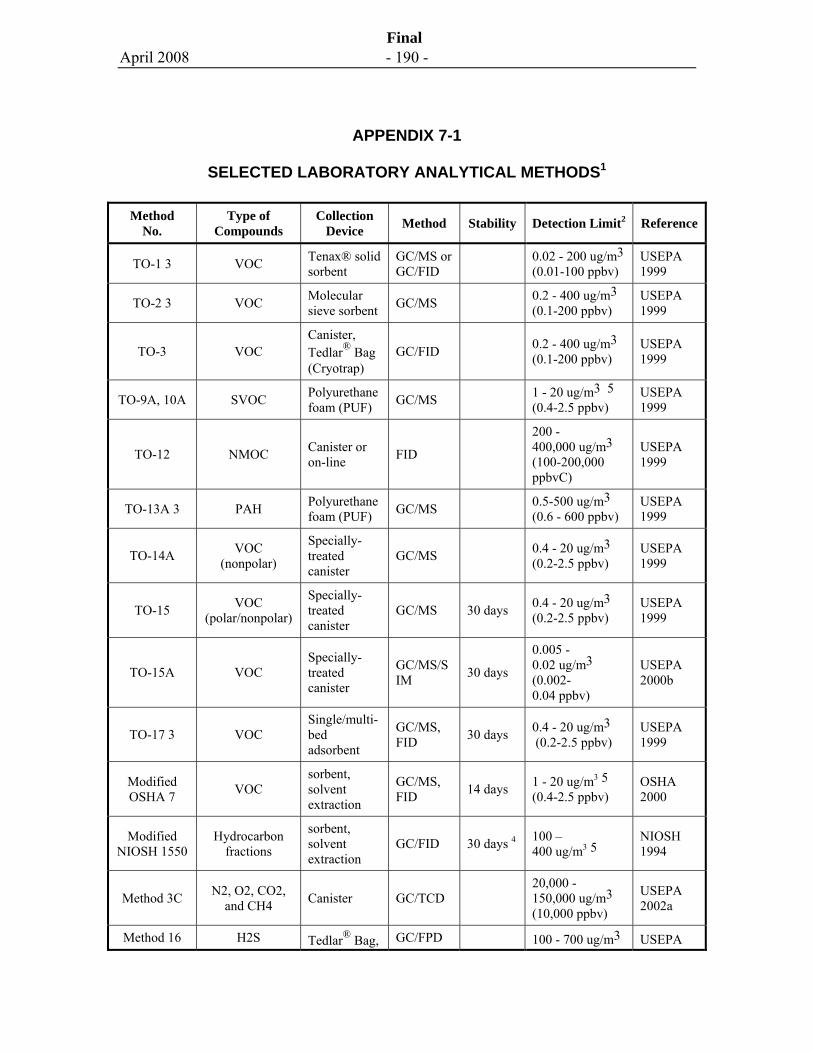
April 2008 - 190 -

Final

APPENDIX 7-1

SELECTED LABORATORY ANALYTICAL METHODS1

Method No.

Type of Compounds

Collection Device Method Stability Detection Limit2 Reference

TO-1 3 VOC Tenax® solid sorbent

GC/MS or GC/FID 0.02 - 200 ug/m3

(0.01-100 ppbv) USEPA 1999

TO-2 3 VOC Molecular sieve sorbent GC/MS 0.2 - 400 ug/m3

(0.1-200 ppbv) USEPA 1999

TO-3 VOC Canister, Tedlar® Bag (Cryotrap)

GC/FID 0.2 - 400 ug/m3 (0.1-200 ppbv)

USEPA 1999

TO-9A, 10A SVOC Polyurethane foam (PUF) GC/MS 1 - 20 ug/m3 5

(0.4-2.5 ppbv) USEPA 1999

TO-12 NMOC Canister or on-line FID

200 - 400,000 ug/m3 (100-200,000 ppbvC)

USEPA 1999

TO-13A 3 PAH Polyurethane foam (PUF) GC/MS 0.5-500 ug/m3

(0.6 - 600 ppbv) USEPA 1999

TO-14A VOC (nonpolar)

Specially-treated canister

GC/MS 0.4 - 20 ug/m3 (0.2-2.5 ppbv)

USEPA 1999

TO-15 VOC (polar/nonpolar)

Specially-treated canister

GC/MS 30 days 0.4 - 20 ug/m3 (0.2-2.5 ppbv)

USEPA 1999

TO-15A VOC Specially-treated canister

GC/MS/SIM 30 days

0.005 - 0.02 ug/m3 (0.002-0.04 ppbv)

USEPA 2000b

TO-17 3 VOC Single/multi-bed adsorbent

GC/MS, FID 30 days 0.4 - 20 ug/m3

(0.2-2.5 ppbv) USEPA 1999

Modified OSHA 7 VOC

sorbent, solvent extraction

GC/MS, FID 14 days 1 - 20 ug/m3 5

(0.4-2.5 ppbv) OSHA 2000

Modified NIOSH 1550

Hydrocarbon fractions

sorbent, solvent extraction

GC/FID 30 days 4 100 – 400 ug/m3 5

NIOSH 1994

Method 3C N2, O2, CO2, and CH4 Canister GC/TCD

20,000 - 150,000 ug/m3 (10,000 ppbv)

USEPA 2002a

Method 16 H2S Tedlar® Bag, GC/FPD 100 - 700 ug/m3 USEPA

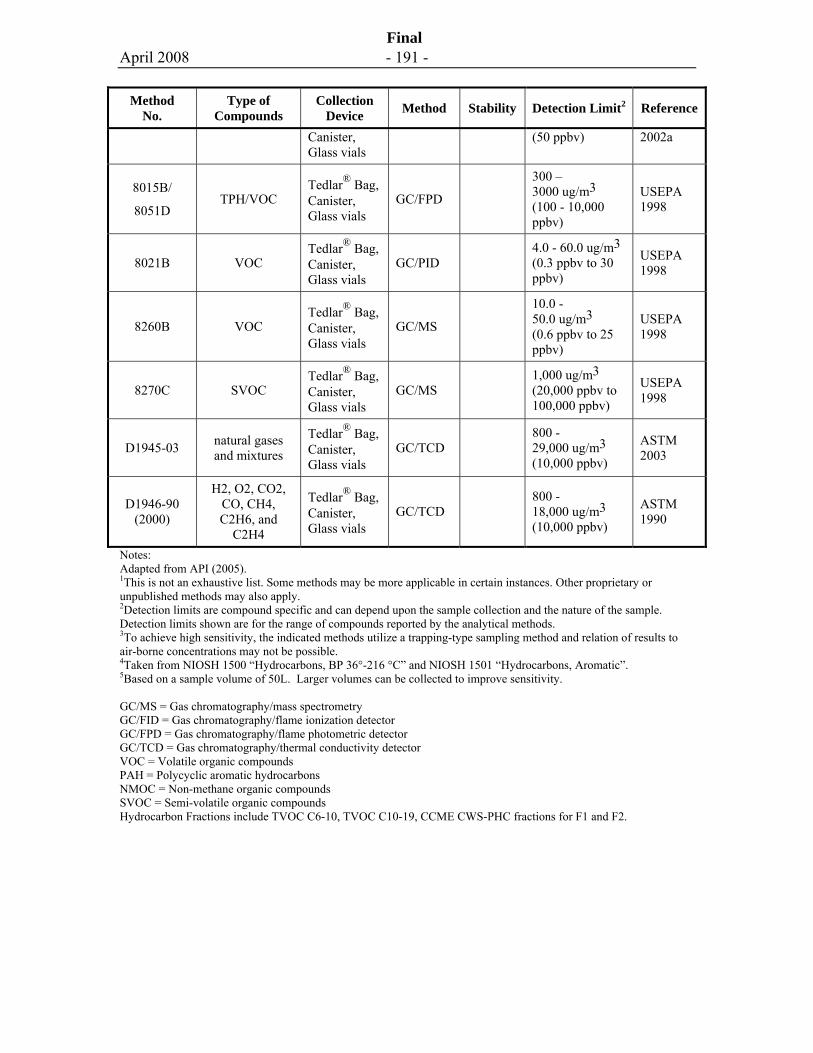
April 2008 - 191 -

Final

Method No.

Type of Compounds

Collection Device Method Stability Detection Limit2 Reference

Canister, Glass vials

(50 ppbv) 2002a

8015B/

8051D TPH/VOC

Tedlar® Bag, Canister, Glass vials

GC/FPD

300 – 3000 ug/m3 (100 - 10,000 ppbv)

USEPA 1998

8021B VOC Tedlar® Bag, Canister, Glass vials

GC/PID 4.0 - 60.0 ug/m3 (0.3 ppbv to 30 ppbv)

USEPA 1998

8260B VOC Tedlar® Bag, Canister, Glass vials

GC/MS

10.0 - 50.0 ug/m3 (0.6 ppbv to 25 ppbv)

USEPA 1998

8270C SVOC Tedlar® Bag, Canister, Glass vials

GC/MS 1,000 ug/m3 (20,000 ppbv to 100,000 ppbv)

USEPA 1998

D1945-03 natural gases and mixtures

Tedlar® Bag, Canister, Glass vials

GC/TCD 800 - 29,000 ug/m3 (10,000 ppbv)

ASTM 2003

D1946-90 (2000)

H2, O2, CO2, CO, CH4, C2H6, and

C2H4

Tedlar® Bag, Canister, Glass vials

GC/TCD 800 - 18,000 ug/m3 (10,000 ppbv)

ASTM 1990

Notes: Adapted from API (2005). 1This is not an exhaustive list. Some methods may be more applicable in certain instances. Other proprietary or unpublished methods may also apply. 2Detection limits are compound specific and can depend upon the sample collection and the nature of the sample. Detection limits shown are for the range of compounds reported by the analytical methods. 3To achieve high sensitivity, the indicated methods utilize a trapping-type sampling method and relation of results to air-borne concentrations may not be possible. 4Taken from NIOSH 1500 “Hydrocarbons, BP 36°-216 °C” and NIOSH 1501 “Hydrocarbons, Aromatic”. 5Based on a sample volume of 50L. Larger volumes can be collected to improve sensitivity. GC/MS = Gas chromatography/mass spectrometry GC/FID = Gas chromatography/flame ionization detector GC/FPD = Gas chromatography/flame photometric detector GC/TCD = Gas chromatography/thermal conductivity detector VOC = Volatile organic compounds PAH = Polycyclic aromatic hydrocarbons NMOC = Non-methane organic compounds SVOC = Semi-volatile organic compounds Hydrocarbon Fractions include TVOC C6-10, TVOC C10-19, CCME CWS-PHC fractions for F1 and F2.

April 2008 - 192 -

Final

APPENDIX 7-2

METHODS FOR HYDROCARBON FRACTIONS

The collection of soil vapour and/or air samples for analysis of hydrocarbon fractions is often required for risk assessments performed in Canada. The hydrocarbon fractions are described in the Canada Wide Standards for Petroleum Hydrocarbon Compounds (CCME, 2008) and consist of the F1 (C6-C10), F2 (C10-C16), F3 (C16-34) and F4 (C34-C50+) fractions, and aliphatic and aromatic subfractions. The aliphatic fractions of interest are C6-C8, C>8-C10, C>10-C12 and C>12-C167. The aromatic fractions of interest are C>7-C88, C>8-C10, C>10-C12 and C>12-C16.

Canisters and Sorbent Tubes by Thermal Desorption Method

When canisters (USEPA TO-15) or thermal tubes (USEPA TO-17) are used, GC/MS analysis must be performed to obtain the aromatic and aliphatic subfractions. When GC/MS is used for analysis of hydrocarbon fractions, differences in MS operation (i.e., full scan versus selective ion mode (SIM)) and the number of and specific ions selected for quantification and calibration will influence the analytical results, which may vary significantly between analytical laboratories depending on the method used. Although quantitative studies have been limited, it appears that a full scan approach where data is obtained on all or most peaks is a more accurate method of quantification compared to SIM mode and quantification of only a limited number of compounds. Unfortunately, CCME (2001) does not prescribe methods for how GC/MS analysis should be performed since it is a soil method involving fractionation and GC/FID analysis.

CCME (2008) defines F1 as the total area summation between the apex of the hexane and decane peaks, and F2 as between the apex of the decane and hexadecane peaks. The BTEX and naphthalene peak areas are removed from the total area summations for each fraction. The F1 is calibrated against toluene response generally obtained as a full scan GC/MS peak. The F2 is typically calculated against decane response as a full scan GC/MS peak. This is a slight deviation from CCME (2001), which indicates the average of the decane and hexadecane response should be used; however, laboratories find it is difficult to generate and maintain a known vapour concentration of hexadecane. Therefore the response of decane only is often used to calibrate for the F2 fraction. For the aliphatic/aromatic subfractions, one option is identify the peaks as being aromatic or aliphatic and then add full scan peak areas (not area summation) of the aliphatic and aromatic peaks within their respective carbon number ranges. Aliphatic subfractions are quantified against the full mass spectra response of n-hexane; aromatics against toluene.

7 In some cases C>16-C21 is also quantified, although the vapour-phase concentrations within this carbon range tend to be negligible. 8 This fraction is comprised mostly of toluene, ethylbenzene and xylenes (TEX) and therefore is sometimes not quantified

April 2008 - 193 -

Final

While CCME (2001) clearly defines the F1 and F2 fractions, no such guidelines exist for subfractions. This has lead to variable and uncertain definitions, for example, the C6-C8 aliphatic fraction is referenced as either C6-C8 or >C6-C8. The first implies including the n-hexane peak in the area summation. The second implies excluding n-hexane. The n-hexane peak should be included in the analysis considering it has a relatively high toxicity.

Sorbent Tubes that are Solvent Extracted

Sorbent tubes that are extracted with a solvent such as carbon disulphide (i.e., modified industrial hygiene methods) allow fractionation using silica gel columns and analysis using GC/FID methods. One method commonly used by laboratories in Canada involves fractionation of the carbon disulphide extract (i.e., sample) using a micro-silica gel column. After adding the carbon disulphide to the column, the column is successively eluted with pentane and a pentane/dichloromethane (60:40) mixture to collect the aliphatic and aromatic fractions, respectively. Each fraction is analyzed by GC/FID method for quantification. This method does not have the sensitivity that the USEPA TO-15 and TO-17 methods have because only a small fraction of the solvent extract is analyzed.

British Columbia Method

In British Columbia, soil vapour and air samples are commonly also analyzed for total volatile organic compound (TVOC) fractions in accordance with provincial regulatory policy. The TVOC (6-10) fraction is identical to CCME F1, except that BTEX is not subtracted from the results. The TVOC (10-19) fraction is similar to CCME F2, except that the cut-off is C19 and not C16, although compounds between C16 and C19 are not expected to be volatile. The naphthalene concentration is not subtracted from the TVOC (10-19).

References

Canadian Council of Ministers of the Environment, 2001. Reference Method for Canada-Wide Standards for Petroleum Hydrocarbon (PHC) in Soil – Tier 1 Method. Publication No. 1310, 2001, Winnipeg.

April 2008 - 194 -

Final

8.0 INDOOR AIR QUALITY TESTING FOR EVALUATION OF SOIL VAPOUR INTRUSION

8.1 Context, Purpose and Scope

This chapter describes methodology for completing indoor air quality (IAQ) testing for evaluation of soil vapour intrusion.9 The testing of IAQ may be warranted when previous phases of an investigation indicate the potential for unacceptable risks from vapour migration into indoor air. The use of IAQ measurements to evaluate potential health risk associated with vapour intrusion is an option for a current exposure scenario (existing building). While indoor air testing can provide a direct measurement of potential inhalation exposure, there are a number of issues that can complicate a risk assessment based on indoor air measurements, and which should be taken into consideration. These issues include background sources of the chemicals of interest and often significant variability observed in indoor vapour concentrations due to building or weather related factors. An IAQ testing program is also a relatively intrusive activity that particularly for a residential or institutional setting requires appropriate communication of program objectives and results.

The basic steps for design of an IAQ program are similar to those described for soil vapour characterization and consist of (1) development of a conceptual site model (CSM), with specific consideration of factors that influence IAQ based on site conditions, (2) development of IAQ study objectives, and (3) preparation of a sampling plan. As indicated for soil vapour characterization, it is not possible to provide a standardized template for IAQ program design, and instead key principles and factors that should be considered in developing a sampling strategy are discussed below. A detailed flow chart of the framework for an IAQ study is provided in Figure 8-1.

Indoor air sampling should be carried out according to an established plan, considering the study objectives and the data quality objectives. However, the plan should be flexible in that if the circumstances change, the plan could be adapted accordingly. In addition, if relevant information is obtained from activities such as the pre-sampling building survey or preliminary screening, the program should be refined to address these changes.

Indoor air quality studies for assessment of soil vapour intrusion typically include some concurrent testing of outdoor air as well as subslab or near building soil vapour testing. Subslab or near building soil vapour samples may be used to identify the contaminants 9 The guidance in this chapter was developed in parallel with similar guidance on indoor air quality testing for Ontario Ministry of Environment and Alberta Environment. As a result there are common elements to all three guidance documents.

Indoor Air Quality (IAQ) Testing

This chapter describes the planning, process and methods for IAQ studies. The key elements and their corresponding sections in the chapter are: Conceptual site model (S 8.2), Study objectives (S 8.3), Sampling approach and design (S 8.3), Indoor air analysis (S 8.4), and Data validation and interpretation (S 8.5).

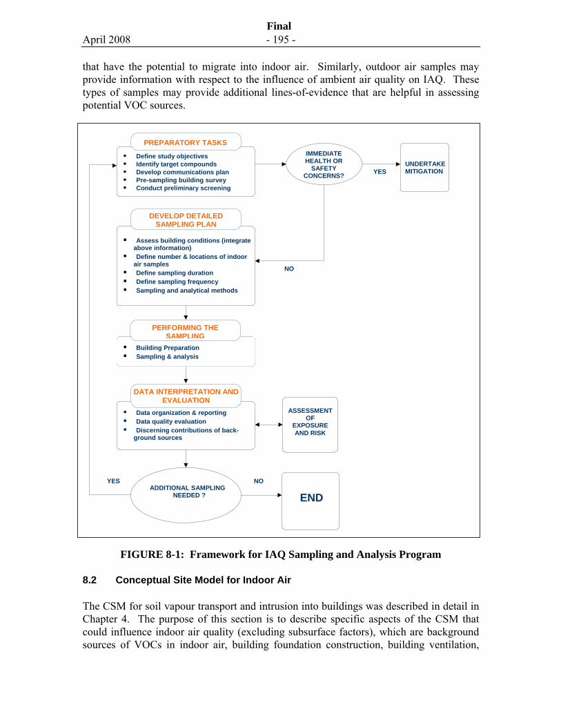
April 2008 - 195 -

Final

that have the potential to migrate into indoor air. Similarly, outdoor air samples may provide information with respect to the influence of ambient air quality on IAQ. These types of samples may provide additional lines-of-evidence that are helpful in assessing potential VOC sources.

FIGURE 8-1: Framework for IAQ Sampling and Analysis Program

8.2 Conceptual Site Model for Indoor Air

The CSM for soil vapour transport and intrusion into buildings was described in detail in Chapter 4. The purpose of this section is to describe specific aspects of the CSM that could influence indoor air quality (excluding subsurface factors), which are background sources of VOCs in indoor air, building foundation construction, building ventilation,

Define study objectives Identify target compounds Develop communications plan Pre-sampling building survey Conduct preliminary screening

PREPARATORY TASKS

Assess building conditions (integrate above information)

Define number & locations of indoor air samples

Define sampling duration Define sampling frequency Sampling and analytical methods

DEVELOP DETAILED SAMPLING PLAN

Building Preparation Sampling & analysis

PERFORMING THE SAMPLING

DATA INTERPRETATION ANDEVALUATION

IMMEDIATE HEALTH OR

SAFETY CONCERNS?

UNDERTAKE MITIGATION

ASSESSMENTOF

EXPOSURE AND RISK

ADDITIONAL SAMPLINGNEEDED ? END

YES NO

NO

YES

Data organization & reporting Data quality evaluation Discerning contributions of back-

ground sources

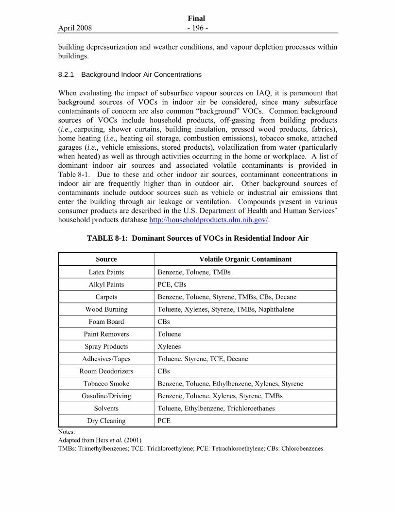
April 2008 - 196 -

Final

building depressurization and weather conditions, and vapour depletion processes within buildings.

8.2.1 Background Indoor Air Concentrations

When evaluating the impact of subsurface vapour sources on IAQ, it is paramount that background sources of VOCs in indoor air be considered, since many subsurface contaminants of concern are also common “background” VOCs. Common background sources of VOCs include household products, off-gassing from building products (i.e., carpeting, shower curtains, building insulation, pressed wood products, fabrics), home heating (i.e., heating oil storage, combustion emissions), tobacco smoke, attached garages (i.e., vehicle emissions, stored products), volatilization from water (particularly when heated) as well as through activities occurring in the home or workplace. A list of dominant indoor air sources and associated volatile contaminants is provided in Table 8-1. Due to these and other indoor air sources, contaminant concentrations in indoor air are frequently higher than in outdoor air. Other background sources of contaminants include outdoor sources such as vehicle or industrial air emissions that enter the building through air leakage or ventilation. Compounds present in various consumer products are described in the U.S. Department of Health and Human Services’ household products database http://householdproducts.nlm.nih.gov/.

TABLE 8-1: Dominant Sources of VOCs in Residential Indoor Air

Source Volatile Organic Contaminant

Latex Paints Benzene, Toluene, TMBs

Alkyl Paints PCE, CBs

Carpets Benzene, Toluene, Styrene, TMBs, CBs, Decane

Wood Burning Toluene, Xylenes, Styrene, TMBs, Naphthalene

Foam Board CBs

Paint Removers Toluene

Spray Products Xylenes

Adhesives/Tapes Toluene, Styrene, TCE, Decane

Room Deodorizers CBs

Tobacco Smoke Benzene, Toluene, Ethylbenzene, Xylenes, Styrene

Gasoline/Driving Benzene, Toluene, Xylenes, Styrene, TMBs

Solvents Toluene, Ethylbenzene, Trichloroethanes

Dry Cleaning PCE Notes: Adapted from Hers et al. (2001) TMBs: Trimethylbenzenes; TCE: Trichloroethylene; PCE: Tetrachloroethylene; CBs: Chlorobenzenes

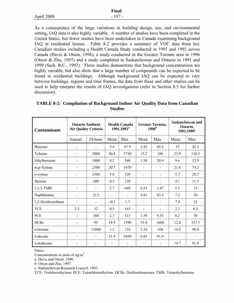
April 2008 - 197 -

Final

As a consequence of the large variations in building design, use, and environmental setting, IAQ data is also highly variable. A number of studies have been completed in the United States, but fewer studies have been undertaken in Canada examining background IAQ in residential homes. Table 8-2 provides a summary of VOC data from key Canadian studies including a Health Canada Study conducted in 1991 and 1992 across Canada (Davis & Otson, 1996), a study conducted in the Greater Toronto area in 1996 (Otson & Zhu, 1997) and a study completed in Saskatchewan and Ontario in 1991 and 1999 (Sask. R.C., 1992). These studies demonstrate that background concentrations are highly variable, but also show that a large number of compounds can be expected to be found in residential buildings. Although background IAQ can be expected to vary between buildings, regions and time frames, the data from these and other studies can be used to help interpret the results of IAQ investigations (refer to Section 8.5 for further discussion).

TABLE 8-2: Compilation of Background Indoor Air Quality Data from Canadian Studies

Ontario Ambient Air Quality Criteria

Health Canada 1991,1992a

Greater Toronto, 1996b

Saskatchewan and Ontario,

1991,1999c Contaminant

Annual 24-hour Mean Max Mean Max Mean Max

Benzene - - 5.4 67.9 3.42 45.8 15 42.3

Toluene - 2000 40.8 5730 15.2 186 23.9 110.5

Ethylbenzene - 1000 8.2 540 1.58 20.9 9.6 32.9

m,p-Xylene - 2300 20.7 1470 - - 21.6 74.2

o-xylene - 2300 5.6 320 - - 5.7 20.3

Styrene - 400 0.3 130 - - 4.1 11.3

1,3,5-TMB - - 2.7 640 0.53 1.47 5.1 15

Naphthalene - 22.5 - - 4.81 83.4 7.2 30

1,2-Dichloroethane - - <0.1 1.7 - - 7.4 25

TCE 2.3 12 0.5 165 - - 2.3 6.5

PCE - 360 2.7 313 1.59 9.55 8.2 30

DCBs - 95 18.9 1390 53.4 1600 12.8 337.5

n-hexane 12000 1.2 124 5.24 108 14.5 99.4

n-decane - - 31.4 6450 6.85 91.9 - -

n-dodecane - - - - - - 14.7 91.9

Notes: Concentrations in units of ug/m3 a: Davis and Otson. 1996. b: Otson and Zhu. 1997. c: Saskatchewan Research Council. 1992. TCE: Trichloroethylene; PCE: Tetrachloroethylene; DCBs: Dichlorobenzenes; TMB: Trimethylbenzene

April 2008 - 198 -

Final

Due to the high potential for detecting VOCs from background sources, particular care must be taken in the collection, review and interpretation of IAQ data. For instance, it is important to understand, as well as minimize, the effects of indoor sources through an assessment of building conditions and proper building preparation prior to sampling (Exhibit 8.1), and in certain cases, include sampling to evaluate representative background air concentrations at the site.

8.2.2 Building Foundation Construction

The building foundation construction will influence soil vapour intrusion rates into the building. For example, soil vapour can migrate through relatively small cracks or openings in the foundation or through utility penetrations. Soil vapour intrusion rates may vary depending on type of foundation, which include basement, slab-on-grade, crawlspace or earthen floor construction. For houses, there is often a perimeter edge crack between the foundation wall and slab for concrete floor slab construction. Compared to houses, construction methods for commercial buildings may be different including some buildings where measures are taken to seal concrete foundations, which would tend to reduce (but perhaps not eliminate) soil vapour intrusion. Utilities represent potential entry points for soil vapour intrusion regardless of building type.

8.2.3 Building Ventilation

Through building ventilation and exchange with fresh air, vapour concentrations in indoor air are usually diluted. Building ventilation or air exchange vary depending on climate, construction and season. A review of approximately 2,800 building ventilation measurements in houses across the U.S. grouped the results according to regions (defined by heating degree-days) and four seasons (Murray and Burmaster, 1995). The average yearly air change per hour (ach) for the four regions ranged from 0.4 ach to 0.98 ach. For the north central to eastern part of the US (which most closely approximates most regions in Canada), the average ach in summer was 0.82 ach, the average in fall was 0.25 ach, the average in winter was 0.36 hr-1 and the average in spring was 0.44 hr-1. In Canada, air exchange rates in high energy efficient (“R-2000”) homes can be quite low based on tight construction (i.e., 0.1 ach to 0.2 ach). In an Ontario study, air exchange rates from 70 houses ranged from 0.06 ach to 0.77 ach, with the lowest air exchange occurring in summer in R-2000 houses with closed windows (Walkinshaw, 1987). In a study completed in Saskatchewan and Tilsonburg, Ontario, the average measured air exchange rate from 44 houses was 0.34 ach (Saskatchewan Research Council, 1992), while in a study completed in the Greater Toronto area, the average air exchange rate from 44 houses was 0.45 ach (Otson and Zhu, 1997).

April 2008 - 199 -

Final

For commercial buildings, design air exchange rates must meet minimum requirements based on building occupancy, although actual ventilation system efficiency may be variable depending on operation of the HVAC system. Standards in Canada and the U.S. both specify minimum ventilation rates for residential and commercial buildings.10 For example, American Society of Heating Refrigerating and Air-Conditioning Engineers (2004) indicates that for office use, 20 standard cubic feet of outdoor air is blown into the building per person to maintain sufficient fresh air supply, which corresponds to an air exchange of about 0.72 ach for typical occupancy. Ventilation rates for institutional buildings are higher. The USEPA Building Assessment, Survery, and Evaluation Study (BASE) of one hundred randomly selected commercial buildings, which represented a wide range in construction, found that the 25th, 50th and 75th percentile air change rates were 0.47 hr-1, 0.98 hr-1 and 2.62 hr1, respectively (National Institute of Standards and Technology, 2004). When conducting a site specific assessment, it may be instructive to obtain information on building ventilation from building HVAC engineers since often design and test information providing data on air flow rates for return and supply air will be available. This informaiton should be considered when developing the IAQ Program.

8.2.4 Building Depressurization and Weather Conditions

The indoor and outdoor temperature, number of storeys, degree of air leakage between floors, and presence of chimney, flues, exhaust fans and vents, may contribute to the pressure differentials that affect the rate of intrusion of soil gas. Of particular importance is the “stack effect” that may occur during the heating season as a result of hot air rising in a building and leaving near the top of the building (e.g., through a chimney, leaky attic, exhaust vent). This creates a negative pressure within the building, thus drawing outdoor air and soil gas into the building through openings within the lower regions of the building (i.e., doors, windows, cracks and/or the building foundation). Pressure differences during the heating season for houses with basements typically range from 2 to 10 Pa, but may be as high as 15 Pa (Figley, 1997; Hers et al., 2001).

The operation of the HVAC system may also result in building depressurization through intake and exhaust systems that are not balanced or through insufficient combustion air. The operation of fans and fireplaces also can result in a depressurized building. For commercial buildings, the HVAC system may be designed to provide for positive pressure under most conditions, but for tall buildings, the stack effect may be sufficient to maintain a negative pressure at ground level during cold weather. Commercial building pressures may also depend on operation of the HVAC system and exhaust fans (e.g., fume hoods, oven vents). The ASTM (2003) for radon mitigation system specifies a pressure differential of 6 to 9 Pascals as sufficient to curtail vapour intrusion, and HVAC units may produce this level of positive pressure. Information on weather (e.g. temperature and barometric pressure) and HVAC operations (e.g. ambient pressure in the area of monitoring) should be collected and interpreted as part of the IAQ program.

10 Examples are CSA F326 and ANSI / ASHRAE Standard 62.1 – 2004 Ventilation for Acceptable Indoor Air Quality.

April 2008 - 200 -

Final

Wind force may create pressure differentials between upwind and downwind sides of the building, which is another mechanism that causes the building interior to be under pressurized. Changes in barometric pressure as a result of meteorological conditions can also cause pressure differences between the building interior and exterior. These pressure differences may occur at varying temporal scales (hourly to seasonally), but in general, the most significant pressure differences occur under severe winter conditions.

Thus, weather conditions and HVAC operation may have a marked effect on air exchange rates and pressure differences between indoor and outdoors, which can both affect the rates of soil vapour intrusion into buildings and the degree of mixing and dilution within the building structure.

8.2.5 Mixing of Vapours Inside Building

Within the building, contaminants will diffuse as a result of chemical gradients and disperse through air movement. Mixing between building floors will depend on the HVAC system and air leakage between floors. Elevator shafts often include a sump and are not ventilated; they may represent points where migration and accumulation of soil vapours could occur. Elevator shafts can also represent conduits for inter-floor migration of vapours.

8.2.6 Vapour Depletion Mechanisms

Chemical or physical mechanisms may result in the removal of vapours from indoor air, in addition to dilution through building ventilation. Since soil vapour intrusion typically occurs over timescales of months to years, the removal of volatiles in air through adsorption onto building materials is unlikely to have a significant long-term effect on indoor vapour concentrations since adsorption sites on building materials will likely be filled over time. Adsorption onto building materials can be reversible (i.e., desorption can occur) and thus should also be considered as a source of volatiles, depending on building conditions. For example, even after soil vapour intrusion is mitigated through a subslab venting system, there may be a period of time over which the chemical of concern is detected in indoor air as a result of desorption from building materials. Chemical transformations due to processes such as photo-oxidation are generally relatively slow processes (i.e., half-lives of days) and biodegradation is unlikely to be a relevant process in an indoor environment.

April 2008 - 201 -

Final

8.3 Development of Indoor Air Quality Study Approach and Design

8.3.1 Define Study Objectives

The study objectives should be well defined prior to developing a sampling plan, as the sampling plan could vary substantially depending on the type of data required and how that data is intended to be used. The primary goal of the indoor air quality study is often to provide data that could be used to evaluate exposure and potential human health risk through inhalation of indoor vapours. To meet this objective, the building conditions and sampling locations should generally reflect typical exposure conditions, as further described below. Samples collected to meet this objective are typically referred to as “exposure” samples.

There may be other specific objectives of the IAQ study that would result in a different sampling strategy. For example, if the goal is to evaluate potential entry points for soil gas into a building, samples may be collected from close to cracks or within utility openings. Samples collected to meet this objective are typically referred to as “pathway” samples. If the objective of the IAQ study is to evaluate the potential influence of background sources of indoor air quality relative to subsurface sources, several indoor air samples from different locations within a building may be required. In addition, the building environment may be artificially controlled at the time IAQ sampling is conducted to assist in evaluation of background sources, as described in Section 8.3.10.

The study objectives can also be broadly defined in terms of the phase or level of investigation. An initial preliminary investigation may consist of a limited number of IAQ samples. If the preliminary investigation indicates a potential indoor air quality concern, a detailed investigation may be required consisting of a greater number of samples. Finally, if vapour intrusion mitigation systems are installed, follow-up IAQ monitoring may be required for some period of time.

8.3.2 Identify Target Compounds

The target compounds for the sampling plan are dependant upon the contaminant source under evaluation. Target compounds would generally include the primary constituents of the contamination source and may also include potential breakdown products of these constituents. In addition to contaminants of potential concern, other compounds that are present as background constituents and that could be useful as tracers should also be considered. For an IAQ study designed to evaluate soil vapour intrusion from contaminated soil or groundwater, a screening process based on volatility and toxicity can be used to identify target compounds (Golder Associates, 2007). Target compounds may also be identified based on the results of previous indoor air sampling at the site or based on the history of the site and/or neighbouring properties.

For petroleum hydrocarbons, target compounds also may include petroleum fractions as well as specific chemicals of potential concern. Specific chemicals are often the more

April 2008 - 202 -

Final

potent chemicals associated with the petroleum fraction and include carcinogenic compounds such as benzene.

8.3.3 Develop Communications Program

An important part of the IAQ program is communication with the building occupants and owners and other stakeholders, to keep them informed and involved in the process. This can be done throughout the sampling process, but is especially important in the preparatory stage. Issues to address with building occupants include: why the study is being conducted and what the study objectives are; scheduling the pre-sampling building survey; discussing the types of activities to avoid prior to the sampling events (see Section 8.3.10); scheduling and discussing the sampling that will be conducted; background sources and issues; and communication of the results of the sampling program. Consideration should be given to the development of an access agreement between parties prior to sampling.

8.3.4 Conduct Pre-Sampling Building Survey

Buildings should be inspected prior to and during IAQ testing to assess whether there are potential background sources of chemicals and also to describe building conditions that may influence indoor air concentrations. Building occupants may also be interviewed to derive additional information on factors that may affect IAQ and to determine the building occupancy characteristics. Examples of a pre-sampling building survey, that could be used to direct a building inspection and occupant interviews, are included in New Jersey Department of Environmental Protection (2005). The pre-sampling building survey may be used as a tool to refine the sampling plan and identify any building preparation activities that should be considered prior to sampling. Such activities might include the removal of consumer products and/or other sources of VOCs from the buildings, if possible. Relevant portions of the survey should be reviewed again at the time indoor air sampling is performed. A survey should be completed for each building being investigated.

8.3.5 Conduct Preliminary Screening

In conjunction with the pre-sampling building survey, a preliminary screening of the study building using a portable air monitoring instrument such as a photoionization detector (PID) can provide useful information on background VOC sources in indoor air. When sensitive PIDs are used (low ppbV range), they may also be capable of identifying entry points where soil gas intrusion is occurring. It is important to note that most direct-measuring instruments measure relative levels of organic compounds as a group and are not capable of identifying specific compounds. Furthermore, for most conventional PIDs/FIDs, the sensitivity of these instruments is often insufficient to detect compounds at levels that may be of concern for human health. These instruments are often used to identify potentially explosive conditions (see 8.3.6. for further discussion). Therefore, while they may be a useful tool for identifying indoor VOC sources or targeting sampling locations at some sites, they may not be used to rule out the presence of background contaminants in indoor air.

April 2008 - 203 -

Final

The PID measurements in some environments may be biased high. For example, condensation on the PID sensor results in a slowly rising false positive response that may reach several hundred ppm (Western Australia Department of Environment, 2005). Microparticles of dust and wood soot absorb moisture more readily than a clean sensor surface exacerbating the effect of moisture; therefore, relevant conditions during sampling should be noted.

8.3.6 Identify Immediate Health or Safety Concerns

If the building survey or preliminary screening identify immediate health or safety concerns associated with chemical odours or where occupants exhibit signs of illness due to inhalation of volatiles in indoor air, the environmental health officer (or other responsible authority) should be notified, and building occupants should be evacuated, as appropriate. Further actions should be taken to identify the chemical source and mitigate the hazard, as warranted. There may also be instances where there are safety concerns associated with the accumulation of potentially explosive levels of volatile chemicals inside or near to buildings.

8.3.7 Define Number and Locations of Indoor and Outdoor Air Samples

The number and locations of indoor air samples will be dictated by several factors. If a preliminary investigation of IAQ is being undertaken, a limited number of samples may be sufficient. If the study objectives require a statistical approach or analysis of results, multiple samples would be required. The building characteristics including size, construction and ventilation patterns will also influence the required number of samples. For example, if the building is a small house with reasonably good ventilation, the indoor air concentrations within the house may be relatively uniform. For this scenario, two samples is initially recommended.

For a larger house, commercial building, or school, where indoor air concentrations may vary in different parts of the building, multiple samples are required to characterize indoor air quality. For a residence with multiple floors, consideration should be given to collecting at least one sample per floor (per sampling event) to characterize inter-floor variability. Where minimal sampling is conducted for a preliminary assessment, it is generally preferable to target the first level of the building (e.g., basement) since vapour concentrations are expected to be highest in lower regions of the building in instances of soil vapour intrusion. Exposure samples should be collected within the typical breathing zone at a height of approximately 1 m to 1.5 m above the floor, preferably near the centre of the room, which is generally representative of overall room conditions.

Outdoor air will influence indoor air quality and may also contain chemicals at concentrations that exceed risk-based concentrations. Therefore, it is good practice to obtain outdoor air samples as part of the IAQ program. The number of samples will be site specific, but several samples obtained from multiple locations may be needed. As part of the outdoor air program, it is also important to identify emission sources such as gasoline stations, major highways, paving operations and remediation systems. It is

April 2008 - 204 -

Final

important to protect outdoor air samplers from the elements (rain or snow) and vandalism.

8.3.8 Define Sampling Duration

The duration for sample collection may depend on the study objectives. The selected sample duration should yield an average concentration of chemicals of potential concern over the expected daily exposure duration. For a residential scenario, it is possible that residents may be present in the home 24 hours per day. Therefore, a 24-hour sample duration is recommended for a residential scenario.11 For a commercial scenario, a sample duration equivalent to the standard 8-hour commercial exposure duration is recommended. However, a longer or shorter sample duration could be selected, if warranted, based on site-specific conditions and site use. When determining the sampling duration, potential limitations in the sampling device should be considered. For example, for sorbent tubes, chemical breakthrough may be an issue depending primarily on the sampling duration and flow rate.

8.3.9 Define Sampling Frequency

The sampling frequency will depend on study objectives, the nature of the contamination source and variability expected due to factors such as building characteristics, weather conditions and occupancy characteristics during sampling. Since it is not possible to accurately predict concentration variability due to the site specific and complex nature of the processes that contribute to soil vapour intrusion, repeat sampling is generally required to establish concentration variability at a given site. In general, a minimum of two sampling events that capture possible seasonal variability (e.g., winter/summer) are required; however, additional sampling events may be warranted at some sites. In general, higher indoor vapour concentrations would be expected when sampling is performed under winter conditions. Repeat sampling may also be warranted, for example, if the subsurface source concentrations are changing over time (e.g., mobile groundwater plume).

11 To provide perspective on sampling duration it is noted that it is generally recommended that radon samples be collected over a period of one week or longer to account for temporal variability (www.epa.gov/radon). Studies of radon provide valuable insight on potential indoor air concentration variability for vapour intrusion. For example, Groves-Kirkby et al. (2006) in a study comparing time-integrated indoor radon sampling for different time scales concluded that natural variability caused many one-week results (compared to three month tests) to be equivocal when compared to action levels, necessitating repetition of the measurement. Continuous radon monitoring indicated roughly diurnal (24-hour) variations that were up to one order-in-magnitude. Font et al. (2001) found that soil moisture levels caused by precipitation caused variations in indoor radon concentrations. The feasibility and need for longer duration active air sampling for evaluation of vapour intrusion is an area of current research.

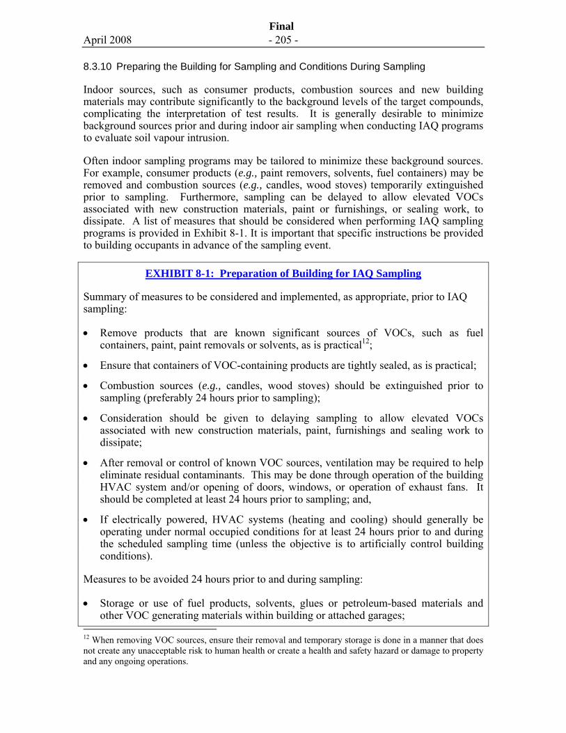
April 2008 - 205 -

Final

8.3.10 Preparing the Building for Sampling and Conditions During Sampling

Indoor sources, such as consumer products, combustion sources and new building materials may contribute significantly to the background levels of the target compounds, complicating the interpretation of test results. It is generally desirable to minimize background sources prior and during indoor air sampling when conducting IAQ programs to evaluate soil vapour intrusion.

Often indoor sampling programs may be tailored to minimize these background sources. For example, consumer products (e.g., paint removers, solvents, fuel containers) may be removed and combustion sources (e.g., candles, wood stoves) temporarily extinguished prior to sampling. Furthermore, sampling can be delayed to allow elevated VOCs associated with new construction materials, paint or furnishings, or sealing work, to dissipate. A list of measures that should be considered when performing IAQ sampling programs is provided in Exhibit 8-1. It is important that specific instructions be provided to building occupants in advance of the sampling event.

EXHIBIT 8-1: Preparation of Building for IAQ Sampling

Summary of measures to be considered and implemented, as appropriate, prior to IAQ sampling:

• Remove products that are known significant sources of VOCs, such as fuel containers, paint, paint removals or solvents, as is practical12;

• Ensure that containers of VOC-containing products are tightly sealed, as is practical;

• Combustion sources (e.g., candles, wood stoves) should be extinguished prior to sampling (preferably 24 hours prior to sampling);

• Consideration should be given to delaying sampling to allow elevated VOCs associated with new construction materials, paint, furnishings and sealing work to dissipate;

• After removal or control of known VOC sources, ventilation may be required to help eliminate residual contaminants. This may be done through operation of the building HVAC system and/or opening of doors, windows, or operation of exhaust fans. It should be completed at least 24 hours prior to sampling; and,

• If electrically powered, HVAC systems (heating and cooling) should generally be operating under normal occupied conditions for at least 24 hours prior to and during the scheduled sampling time (unless the objective is to artificially control building conditions).

Measures to be avoided 24 hours prior to and during sampling:

• Storage or use of fuel products, solvents, glues or petroleum-based materials and other VOC generating materials within building or attached garages;

12 When removing VOC sources, ensure their removal and temporary storage is done in a manner that does not create any unacceptable risk to human health or create a health and safety hazard or damage to property and any ongoing operations.

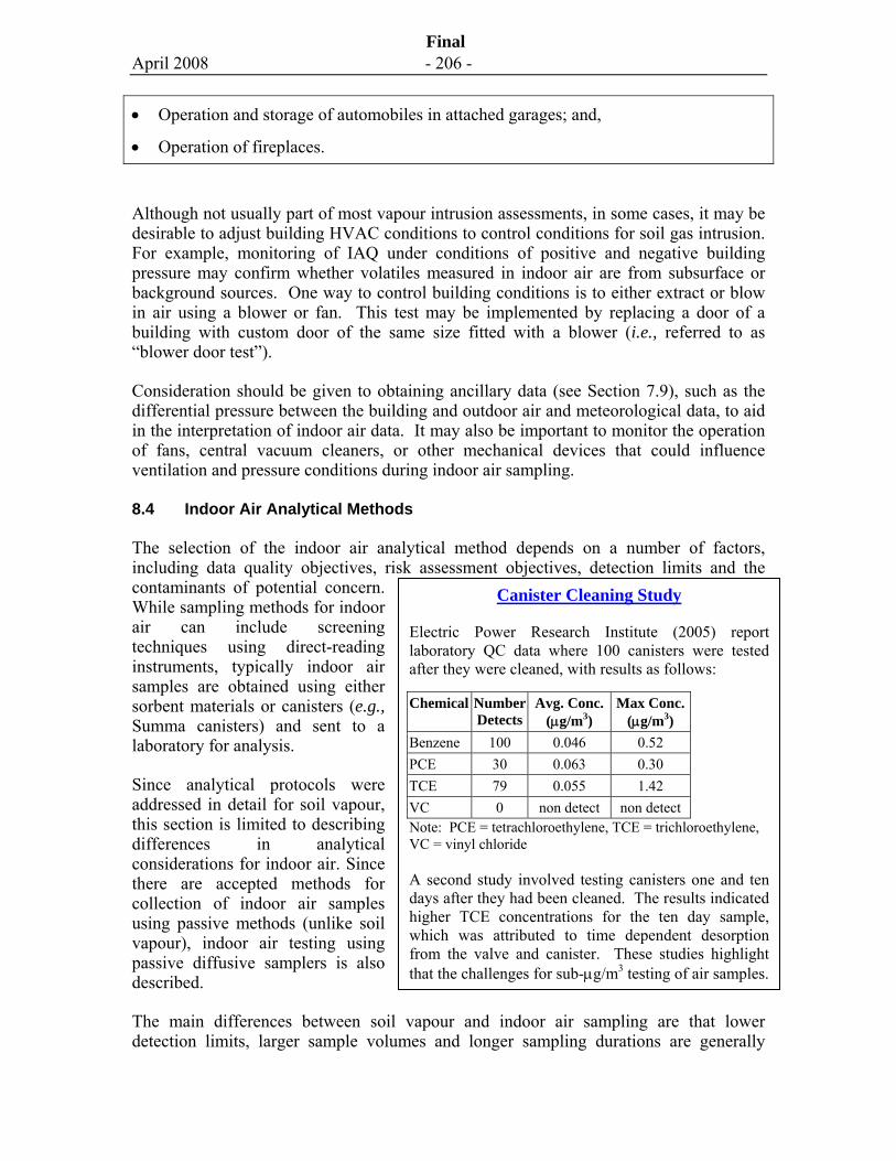
April 2008 - 206 -

Final

• Operation and storage of automobiles in attached garages; and,

• Operation of fireplaces.

Although not usually part of most vapour intrusion assessments, in some cases, it may be desirable to adjust building HVAC conditions to control conditions for soil gas intrusion. For example, monitoring of IAQ under conditions of positive and negative building pressure may confirm whether volatiles measured in indoor air are from subsurface or background sources. One way to control building conditions is to either extract or blow in air using a blower or fan. This test may be implemented by replacing a door of a building with custom door of the same size fitted with a blower (i.e., referred to as “blower door test”).

Consideration should be given to obtaining ancillary data (see Section 7.9), such as the differential pressure between the building and outdoor air and meteorological data, to aid in the interpretation of indoor air data. It may also be important to monitor the operation of fans, central vacuum cleaners, or other mechanical devices that could influence ventilation and pressure conditions during indoor air sampling.

8.4 Indoor Air Analytical Methods

The selection of the indoor air analytical method depends on a number of factors, including data quality objectives, risk assessment objectives, detection limits and the contaminants of potential concern. While sampling methods for indoor air can include screening techniques using direct-reading instruments, typically indoor air samples are obtained using either sorbent materials or canisters (e.g., Summa canisters) and sent to a laboratory for analysis.

Since analytical protocols were addressed in detail for soil vapour, this section is limited to describing differences in analytical considerations for indoor air. Since there are accepted methods for collection of indoor air samples using passive methods (unlike soil vapour), indoor air testing using passive diffusive samplers is also described.

The main differences between soil vapour and indoor air sampling are that lower detection limits, larger sample volumes and longer sampling durations are generally

Canister Cleaning Study

Electric Power Research Institute (2005) report laboratory QC data where 100 canisters were tested after they were cleaned, with results as follows:

Chemical Number Detects

Avg. Conc. (μg/m3)

Max Conc. (μg/m3)

Benzene 100 0.046 0.52 PCE 30 0.063 0.30 TCE 79 0.055 1.42 VC 0 non detect non detect Note: PCE = tetrachloroethylene, TCE = trichloroethylene, VC = vinyl chloride

A second study involved testing canisters one and ten days after they had been cleaned. The results indicated higher TCE concentrations for the ten day sample, which was attributed to time dependent desorption from the valve and canister. These studies highlight that the challenges for sub-μg/m3 testing of air samples.

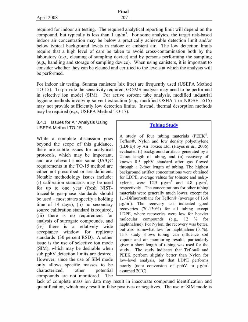
April 2008 - 207 -

Final

required for indoor air testing. The required analytical reporting limit will depend on the compound, but typically is less than 1 ug/m3. For some analytes, the target risk-based indoor air concentration may be below a practically achievable detection limit and/or below typical background levels in indoor or ambient air. The low detection limits require that a high level of care be taken to avoid cross-contamination both by the laboratory (e.g., cleaning of sampling device) and by persons performing the sampling (e.g., handling and storage of sampling device). When using canisters, it is important to consider whether they can be cleaned and certified to the levels at which the analysis will be performed.

For indoor air testing, Summa canisters (six litre) are frequently used (USEPA Method TO-15). To provide the sensitivity required, GC/MS analysis may need to be performed in selective ion model (SIM). For active sorbent tube analysis, modified industrial hygiene methods involving solvent extraction (e.g., modified OSHA 7 or NIOSH 5515) may not provide sufficiently low detection limits. Instead, thermal desorption methods may be required (e.g., USEPA Method TO-17).

8.4.1 Issues for Air Analysis Using USEPA Method TO-15

While a complete discussion goes beyond the scope of this guidance, there are subtle issues for analytical protocols, which may be important, and are relevant since some QA/QC requirements in the TO-15 method are either not prescribed or are deficient. Notable methodology issues include: (i) calibration standards may be used for up to one year (fresh NIST-traceable gas-phase standards should be used – most states specify a holding time of 14 days), (ii) no secondary source calibration standard is required, (iii) there is no requirement for analysis of surrogate compounds, and (iv) there is a relatively wide acceptance window for replicate standards (30 percent RSD). Another issue is the use of selective ion mode (SIM), which may be desirable when sub ppbV detection limits are desired. However, since the use of SIM mode only allows specific masses to be characterized, other potential compounds are not monitored. The lack of complete mass ion data may result in inaccurate compound identification and quantification, which may result in false positives or negatives. The use of SIM mode is

Tubing Study

A study of four tubing materials (PEEK®, Teflon®, Nylon and low density polyethylene (LDPE)) by Air Toxics Ltd. (Hayes et al., 2006) evaluated (i) background artifacts generated by a 2-foot length of tubing, and (ii) recovery of known 0.5 ppbV standard after gas flowed through a 2-foot length of tubing. The highest background artifact concentrations were obtained for LDPE; average values for toluene and m&p-xylene, were 12.5 μg/m3 and 4.8 μg/m3, respectively. The concentrations for other tubing materials were generally much lower, except for 1,1-Difluoroethane for Teflon® (average of 13.8 μg/m3). The recovery test indicated good recoveries (70-130%) for all tubing except LDPE, where recoveries were low for heavier molecular compounds (e.g., 12 % for naphthalene). For Nylon, the recovery was better, but also somewhat low for naphthalene (31%). This study shows tubing can influence soil vapour and air monitoring results, particularly given a short length of tubing was used for the study. The study indicates that Teflon® and PEEK perform slightly better than Nylon for low-level analysis, but that LDPE performs poorly (note conversion of ppbV to μg/m3 assumed 20oC).

April 2008 - 208 -

Final

not recommended during the initial site characterization phase. The specifications for tuning and data acquisition of the GC/MS are important when analyzing in SIM mode. While there is not agreement between laboratories on tuning protocols, in some cases, the protocol developed by the State of Colorado has been adopted (Colorado, 2004).

It is recommended that the laboratory demonstrate how their implementation of the TO-15 method addresses the above quality control issues. Consideration could also be given to requiring that the laboratory be certified under for example the US National Environmental Laboratory Accreditation Program (NELAP) or a provincial or state program.

8.4.2 Issues for Air Analysis using Passive Diffusive Badge Samplers

The use of passive diffusive badge samplers is a common method for evaluation of workplace exposures to VOCs. Typically, these badge-type samplers are used to evaluate exposures in the high part per billion (ppbV) to part per million (ppmV) range over an 8-hour period, although they can be deployed for longer periods of time (up to one week) to evaluate lower concentrations. The absorbent medium is typically charcoal, which is extracted using solvent (carbon disulphide) and analyzed using GC/MS methods (GC/FID is not recommended). Passive samplers are easy to use and do not require a sampling pump.

The sampling (i.e., diffusive uptake) rate is a function of the diffusive coefficient, which is compound and sorbent specific, and the geometry of the sampler. Other factors that affect performance include temperature, pressure, humidity, air velocity and transient changes in contaminant concentrations. More recently, passive diffusive badges have been used for indoor air quality studies involving longer sampling periods and lower detection limits. The use of sorbents that are thermally desorbed (Chromosorb 106, Carbotrap Z) has also recently been investigated (OSHA, 2003). For example, McClenny et al. (2005) report on the results of a thermal desorption method involving a larger volume sampler (SKC Ultra-II) filled with Carbotrap C, where compound-specific method detection limits on the order of 0.03 ppbV to 0.3 ppbV were reported. Another new development is Radiello®, a radial symmetry diffusive sampler, filled with a thermally desorbable graphitised carbon (Bruno et al., 2004).

There are several potential limitations associated with passive diffusive sampling methods that should be recognized:

• The sampling rate is compound specific; there are varying (up to four) levels of validation studies. The highest level of validation are laboratory testing programs designed to evaluate the stability of the sampling rate under varying conditions and contaminant mixtures, whereas the lowest level are estimates from the diffusion coefficient of the analyte;

April 2008 - 209 -

Final

• The sampling rate is typically relatively stable over a certain time interval, but will decrease once saturation of the media is approached; this effect is more pronounced for more volatile VOCs and weaker adsorbants.

• In stagnant air, the sampling rate will decrease; one study indicated a significant decline for sampling face air velocities that were less than 50 cm/s (OHSA, 1998). Another study indicated that badges performed satisfactorily down to face velocities as little as 5 cm/sec, but reported that face velocities inside houses are typically less than 2.5 cm/sec indicating the potential for a “starvation” effect (SKC, 2006); A review of 28 studies between 1973 and 2003 where the effect of face velocity on sampling rate was evaluated indicated that except for one study, significant underestimation in sampling rate was reported (about 20 to 60%) in the wind velocity range encountered in the indoor environment (Lee and Yun, 2004).

• Back-diffusion of compounds out of the sampler may occur for some compounds;

• Humidity above 50 percent will reduce recovery of certain compounds such as vinyl chloride, acetone and methyl ethyl ketone (3M Bulletin 1028, 2000);

• Extraction recovery varies depending on compound; project specific recovery tests are recommended by some badge manufacturers (3M Bulletin 1028, 2000) to address varying recovery for contaminant mixtures;

• There is an absence of established methods for low-level VOC analysis and studies involving longer sampling durations; and,

• Detection limits for passive diffusion samplers typically exceed 0.5 to 1.5 μg/m3 for common VOCs.13

Comparisons of active and passive samplers indicate variable results, with some studies indicating good comparisons between two methods with environmental factors having no significant influence on the results (Strandberg et al., 2005), while other studies report a downward bias in concentrations measured using passive samplers relative to active methods (Jia et al., 2007).

Due to the above limitations, the use of passive badge samplers are not recommended for low or sub-ppbV indoor air quality testing, unless efforts are taken to validate the method based on the anticipated chemicals of concern.

13 Recent developments in passive testing technology allow detection limits as low as 0.05 μg/m3 for set of VOCs (personnel communication, Heidi Hayes, Air Toxics, October 12, 2007).

April 2008 - 210 -

Final

8.5 Data Interpretation and Analysis

8.5.1 Data Organization and Reporting

The indoor air quality data should be tabulated and plotted to facilitate evaluation and review of data relationships and trends. The following data organization and presentation is recommended:

• Tabulate all data including sample location identifier, sample date, sample height, sample location within room, sampling methods, chemical analysis methods, laboratory detection limits and results of chemical analysis.

• Calculate constituent ratios and evaluate trends with respect to (i) indoor air to soil vapour or subslab vapour samples, (ii) first building level to higher level air samples, and (iii) indoor air to outdoor air samples.

• Note building size, foundation conditions, utility penetrations through floor, sumps and drains, attached garages, and stains on floor.

• Note weather conditions, and building HVAC conditions during indoor air sampling and qualitatively describe opening of windows and doors, operation of fireplace, furnace and fans.

• Note potential significant indoor sources of VOCs present during sampling.

• Identify target risk-based indoor air concentrations and background indoor and outdoor air concentration, where available.

8.5.2 Data Quality Evaluation

Following receipt of the indoor air testing results, the data should be evaluated to determine whether they meet data quality objectives outlined in the sampling plan. The data quality analysis for indoor air is similar to soil vapour (Section 7.7.5).

8.5.3 Methods for Discerning Contributions of Background from Indoor Sources

There are a large number of background sources of VOCs including indoor sources such as building materials and consumer products, and outdoor ambient air sources. Since the intent of this guidance is to evaluate impacts to indoor air resulting from soil vapour intrusion, careful consideration must be given to determining which constituents are derived from background sources and which are likely related to the contaminant release or spill. To the extent possible, multiple lines-of-evidence should be considered when evaluating IAQ data. By relying on several lines-of-evidence rather than a single line-of-evidence, the overall level of uncertainty of the study can be reduced.

The relative importance of various lines-of-evidence should be based on professional judgment and should consider site conditions, data quality, as well as an understanding of

April 2008 - 211 -

Final

background sources of contamination, factors affecting IAQ as well as contaminant fate and transport mechanisms.

Subslab Data

Subslab vapour measurements can be an effective means for evaluation of the vapour intrusion potential. When subslab concentrations are similar to or less than the indoor air concentrations it is reasonable to conclude that background sources are likely the source of the chemicals measured in indoor air. When the subslab concentrations are significantly higher than the air concentrations (i.e., about two orders-of-magnitude or higher), than there is a significant potential for vapour intrusion, although this not a definitive indication since there will be variable attenuation in concentrations between subslab and indoor air. The potential downfall of this method is that there can be significant variability in subslab vapour concentrations and therefore the potential for non-representative data.

Constituent Ratios

An evaluation of the ratios between contaminant concentrations in groundwater, soil vapour, indoor air and outdoor air for concurrent data and chemicals with similar fate and transport properties can assist in discerning background sources of contaminants. Chemical ratios in indoor air and soil vapour should be similar if vapour intrusion is the cause for the elevated indoor air concentrations. If the ratios are significantly different (e.g., by more than one order-of-magnitude), there are likely background contributions of VOCs for some or all the chemicals under consideration.

Ratios of more than two compounds can be inspected using multi-linear diagrams (e.g., tri-linear), where the concentrations of each chemical are plotted on an axis and where lines are drawn to connect the plotted points. Depending on the source, the outline may have a characteristic shape. If groundwater data are used, adjustments should be made to take into account different relative volatilities between contaminants (i.e., corrected for varying Henry’s Law constants).

The constituent ratio analysis works best for chemical groups with similar physical-chemical and fate properties, such as tetrachloroethylene and trichloroethylene. Where there are potential significant differences in biodegradation rates, this technique is less effective.

Marker Chemicals

Marker chemicals are compounds which are associated with the subsurface contamination, but not background air sources. An example of a marker chemical is 1,1-dichloroethylene (DCE), which is a degradation product of 1,1,1- trichloroethane and trichloroethylene, and which is not known to be present as background chemical in indoor air. Therefore, detectable levels of 1,1-DCE in indoor air would suggest soil vapour intrusion is occurring (unless from an ambient air source). Marker chemicals, if

April 2008 - 212 -

Final

present, are also useful compounds when evaluating constituent ratios using the method described above.

Spatial Trends

An evaluation of spatial trends may provide insight on differentiating background sources from the contaminants of interest. For instance, VOC concentrations in a basement may be higher than in upper floors. This provides support for a subsurface vapour source, but care must be taken to ensure that the results were not biased by products stored in the basement. Also, testing of “pathway” samples collected near foundation cracks, unsealed utility entry points or other possible preferential transport zones could be compared to samples collected at other parts of the building. Concentrations in pathway samples that are elevated relative to concentrations in samples from other parts of the building may indicate soil vapour intrusion is occurring. However, spatial differences may be minimal in buildings with efficient ventilation systems.

For larger spatial trends, it may be possible to examine the results of indoor air testing for multiple buildings and compare this to known subsurface conditions (e.g., contoured groundwater or soil vapour plume, location of hot spots, depth of groundwater). Buildings located outside the plume may also be used as “reference” sites to establish typical background IAQ (refer to the following section).

Comparison of Indoor Air Data to Literature Background Concentrations

Indoor air quality data may be compared to published data on indoor air quality. Typical background sources and concentrations of VOCs in indoor air were discussed in Section 8.2.1. The data should be compared to data for buildings of similar type (e.g., single family residence, apartment, commercial).

The ratio of measured indoor to outdoor air (I/O) concentration may also be compared to literature values. For some chemicals (e.g., benzene), the I/O ratio is normally relatively close to one (Hers et al., 2001); therefore, large divergences may suggest a subsurface vapour source.

Comparison of Indoor Air Data to Control Building Survey

The IAQ data from buildings above the contaminated area may be compared to IAQ data from nearby “reference” buildings outside the contaminated area. This method requires a sufficient number of buildings to be tested such that statistical comparisons between data sets can be made. There are a number of confounding factors that could contribute to differences in air quality unrelated to soil vapour intrusion. To the extent possible, building construction and occupant usage of the reference buildings should be similar to the buildings under investigation.

April 2008 - 213 -

Final

Modification of Building Pressurization

Indoor air quality testing under positive and negative building pressurization can be used to determine whether soil vapour intrusion is occurring and to evaluate the possible influence of background sources on indoor air quality. Indoor air concentrations that are significantly different under positive and negative pressures suggest vapour intrusion is occurring, since typically, soil gas advection caused by building depressurization is the main cause for soil vapour intrusion. Building pressures can be modified through control of the building HVAC system and use of temporary fans or blowers. While modification of building pressurization goes beyond the typical scope of testing for IAQ studies, it could be considered when it is important to distinguish background from possible subsurface vapour sources.

Comparison of Measurements to Empirical Data and/or Modeling Results

Where there is relatively high confidence in the data and where representative spatially- and temporally-averaged attenuation ratios can be calculated for a building, the internal consistency between measurements and empirical and/or modeling data can be evaluated. For non-degrading chemicals, the upper range in empirical attenuation factors are approximately 10-3 for groundwater-to-indoor air, 10-2 for soil vapour-to-indoor air (for representative data as defined in Chapter 7) and 10-1 for subslab vapour-to-indoor air (Golder, 2007). A measured ratio that exceeds these empirical ratios by a significant degree may suggest a background component. Site-specific modeling may also be performed, for example using the Johnson and Ettinger (1991) model. When there is good quality input data, the modeled and measured values can be expected to agree within about an order-of-magnitude (Hers et al., 2003; Abreu and Johnson et al., 2005; EPRI, 2005). When using this approach, caution must be taken in that the conceptual site model must be well understood and data adequacy and quality must be high. Comparisons using the Johnson and Ettinger model may not be meaningful if there are conditions that fall outside of the processes included in the Johnson and Ettinger model such as preferential pathways, barometric pumping or biodegradation.

8.6 Resources and Weblinks

Compared to soil and groundwater, there are much fewer state-of-the-art guidance documents and resources available on indoor air sampling and analysis. Useful information is provided in the following references.

Interstate Technology and Regulatory Council (ITRC). The Vapor Intrusion Pathway: A Practical Guide (VI-1)(January 2007, 173 pages) provides a generalized framework for evaluating the vapour intrusion pathway and describes the various tools available for investigation, data evaluation, and mitigation. The Vapor Intrusion Pathway: Investigative Approaches for Typical Scenarios (VI-2) (January 2007, 52 pages) is a supplement to Vapor Intrusion Pathway: A Practical Guide. The supplement describes applicable approaches for evaluating the vapor intrusion pathway in six typical

April 2008 - 214 -

Final

scenarios. http://www.itrcweb.org/Documents/VI-1.pdf . http://www.itrcweb.org/Documents/VI-1A.pdf

American Petroleum Institute (API). A Practical Strategy for Assessing the Subsurface Vapor-to-Indoor Air Migration Pathway at Petroleum Hydrocarbon Sites (November 2005) includes guidance on soil gas sampling approach, methods and analysis (November, 2005). http://www.api.org/ehs/groundwater/lnapl/soilgas.cfm

New Jersey Department of Environmental Protection. Vapour Intrusion Guidance (October, 2005). This guidance includes comprehensive methods for site characterization, including soil gas sampling and analysis. http://www.state.nj.us/dep/srp/guidance/vaporintrusion/vig.htm

Massachusetts Department of Environmental Protection. Indoor Air Sampling and Evaluation Guide (April, 2002). http://www.state.ma.us/dep/ors/orspubs.htm#air

8.7 References

Abreu, L. and P.C. Johnson, 2005. Effect of Vapor Source-Building Separation and Building Construction on Soil Vapor Intrusion as Studied with a Three-Dimensional Model. Environ. Sci. Technol., 39, 4550-4561.

American Society for Testing Materials (ASTM), 2003. ASTM Standard E-2121. Standard Practice for Installing Radon Mitigation Systems in Existing Low-Rise Residential Buildings. February 10.

American Society of Heating Refrigerating and Air-Conditioning Engineers, Inc. (ASHRAE), 2001. ANSI/ASHRAE Standard 62-2001. Ventilation for Acceptable Indoor Air Quality.

Bruno, P., M. Caputi, M. Caselli and G. de Gennaro. 2004. Reliability of a BTEX radial diffusive sampler for thermal desorption: field measurements Atmospheric Environmental, 39 (7), March, 1347-1355.

Colorado Department of Public Health and Environment (DPHE), 2004. Draft Indoor Air Guidance. September.

Davis, C.S. and R. Otson, 1996. Estimation of Emissions of Volatile Organic Compounds (VOCs) from Canadian Residences. Volatile Organic Compounds in the Environment, ASTM STP 1261.

Electric Power Research Institute (EPRI), 2005. Reference Handbook for Site-Specific Assessment of Subsurface Vapor Intrusion in Indoor Air. Palo Alto, California, 1008492.

April 2008 - 215 -

Final

Figley, D.A. A Guide for Estimating Indoor Concentrations of Soil Gas Pollutants in Houses. Prepared for CMHC, 1997.

Font, L.L; C. Baixeras, C. And C. Domingo, 2001. Uncertainty, Variability, and Sensitivity Analysis Applied to the RAGENA Model of Radon Generation, Entry, and Accumulation Indoors; Sci. Total Environ. 272, 25-31.

Golder Associates Ltd. 2007. Soil Vapour Intrusion Guidance for Screening Level Risk Assessment (SLRA) (Draft- in progress). Prepared for Health Canada. November.

Groves-Kirkby, C.J., C.J., Denman, A.R., Crockett, R.G.M., Phillips, P.S., Woolridge, A, Gillmore, G.K., 2006. Time-Integrating Radon Gas Measurements in Domestic Premises: Comparison of Short-, Medium and Long-Term Exposures, J.Environ. Radioactivity, 2006, 86 (1), 92-109.

Hayes, H., D.J. Benton and N. Khan, 2006. The Impact of Sampling Media on Soil Gas Measurements. Proc. Of AWMA Vapor Intrusion – The Next Great Environmental Challenge – An Update, September 13-15, Los Angelos, California.

Hayes, H., D.J. Benton, S. Grewal and N. Khan, 2007. Evaluation of Sorbent Methodology for Petroleum-Impacted Site Investigations. Proc. Of AWMA Vapor Intrusion – Learning from the Challenges, September 25-27, Providence, Rhode Island.

Hers, I., Zapf-Gilje, R., Johnson, P.C. and Li, L. 2003. Evaluation of the Johnson and Ettinger model for prediction of indoor air quality. Ground Water Monitoring and Remediation, Summer 2003.

Hers, I., R. Zapf-Gilje, L. Li, L. and J. Atwater, 2001. The use of indoor air measurements to evaluate exposure and risk from subsurface VOCs. J. Air & Waste Manage. Assoc. 51: 174-185.

Jia, C.S, Batterman and C. Godwin. 2007. Continuous, intermittent and passive sampling of airborne VOCs. J. of Enviro. Monit. 9. 1220 -1230.

Johnson, P.C. 2005. Identification of application-specific critical inputs for the 1991 Johnson and Ettinger vapor intrusion algorithm. Groundwater Monitoring & Remediation, 25(1): 63-78.

Johnson, P.C. and R. Ettinger 1991. Heuristic Model for Predicting the Intrusion Rate of Contaminant Vapours into Buildings. Environmental Science and Technology, 25 #8, 1445-1452.

April 2008 - 216 -

Final

Lee, K. and M. Yun 2004. Effect of Face Velocity on Measurement of Passive Samplers. Samplers, Proc. of American Industrial Hygience Association Conference, May 8-13, 2004, Atlanta, Georgia, USA.

McClenny, W.A., Oliver, K.D., Jacumin, H.H., Jr., and Daughtrey, E.H. and Whitaker, J. 2005. 24-Hour diffusive sampling of toxic VOCs in air onto Carbopack X solid adsorbant followed by thermal desorption GC/MS Analysis – Laboratory studies. Environ. Monit., 7, 248-256.

Murray, D.M. and D.E. Burmaster. 1995. Residential air exchange rates in the United States: empirical and estimated parametric distributions by season and climatic region. Risk Anal. 1995. 15:459-465.

National Institute of Standards and Technology (NIST) 2004. Analysis of Ventilation Data from the U.S. Environmental Protection Agency Building Assessment Survey and Evaluation (BASE) Study, Prepared by Andrew Persily and Josh Gorfain, NISTIR Report 7145.

New Jersey Department of Environmental Protection (NJDEP), 2005. Vapour Intrusion Guidance, October.

Occupational Safety and Health Administration (OHSA), 2003. Performance of SKC Ultra Passive Samplers Containing Carboxen 1016, Carbortap Z, or Chromosorb 106 When Challenged With a Mixture Containing Twenty of OSHA SLTC’s Top Solvent Analytes. Prepared by Warren Hendricks for Organic Methods Evaluation Branch, OSHA Salt Lake Technical Center, Salt Lake City, Utah 84115-1802. February.

Occupational Safety and Health Administration (OHSA), 1998. Determination of the Sampling Rate Variation for SKC 575 Series Passive Samplers. Prepared by Warren Hendricks for Organic Methods Evaluation Branch, OSHA Salt Lake Technical Center, Salt Lake City, Utah 84115-1802. April.

Otson, R. and J. Zhu. 1997. I/O Values for Determination of the Origin of Some Indoor Organic Pollutants. Proc. Air & Waste Managements Association’s 90th Annual Meeting and Exhibition, Toronto, Ontario, Canada, June 8 to 13, 1997.

Saskatchewan Research Council (SRC), 1992. Volatile Organic Compound Survey and Summarization of Results. Report I-4800-1-C-92. Prepared for Canada Mortgage and Housing Corporation. April.

SKC, 2006. Measuring sub-ppb levels of VOCs in Indoor Air. Technical Note. Publication 1720, Issue 0611.

Strandberg, B., A. Sunesson, K. Olsson, J. Levin, G. Ljungqvist, M. Sundgren, G, Sallsten and L. Barregard, 2005. Evaluation of two types of diffusive samplers and

April 2008 - 217 -

Final

adsorbents for measuring 1,3-butadience and benzene in air. Atmospheric Environment, 39, 39 (22), July, 4101-1440.

Walkinshaw, D.S. 1987. Indoor Air Quality in Cold Climates: Hazards and Abatements Measures Summary of an APCA International Speciality Conference, J. Air Pollut. Control Assoc., 36, 235-241.

Western Australia Department of Environment 2005. Wagerup 2003 (PID) Ambient Air Sampling Program. June 2005.

3M Technical Data Bulletin, 2000. Organic Vapor Monitor Sampling and Analysis Guide (1028); 3M: St. Paul, MN, 2000. Available at: http:// www.3m.com/intl/ca/english/market/traffic/ohes/pdf_pub/1028.pdf (accessed 2006).

April 2008 - 218 -

Final

9.0 ACRONYMS

ACH air change per hour AEC area of environmental concern API American Petroleum Institute APHA American Public Health Association APEC Area of Potential Environmental Concern AST Above Ground Storage Tank ASTM American Society Testing Materials AAP atomic adsorption spectrometry ATSDR US Agency for Toxic Substances and Disease Registry bgs below ground surface BTEX benzene, toluene, ethylbenzene and xylenes CAEAL Canadian Association for Environmental Analytical Laboratories CCV Continuing Calibration Verification CPPI Canadian Petroleum Producers Institute CPT cone penetrometer test CCME Canadian Council of Ministers of the Environment CEQG Canadian Environmental Quality Guidelines CEAA Canadian Environmental Assessment Act CEM conceptual exposure model CH4 Methane CO2 Carbon Dioxide COPC contaminant of potential concern CSM conceptual site model CSA Canadian Standards Association CV coefficient of variation (standard deviation divided by mean), same as

relative standard deviation) CWS-PHC Canadian Wide Standards - Petroleum Hydrocarbon Compounds (CCME

guidance) DQI data quality indicators DNAPL dense non-aqueous phase liquid (more dense than water) DRA detailed risk assessment ECD electron capture detector F2 Petroleum Hydrocarbons in the carbon range of C11-16 (CCME) F3 Petroleum Hydrocarbons in the carbon range of C17-34 (CCME) F4 Petroleum Hydrocarbons in the carbon range of C35+ (CCME) FID flame ionization detector GC/FID gas chromatography/flame ionization detection GC/MS gas chromatography/mass spectrometry HI hazard index (sum of HQs) HQ hazard quotient HVAC heating, ventilation and air conditioning IAQ indoor air quality I.D. inside diameter INAC Indian and Northern Affairs Canada

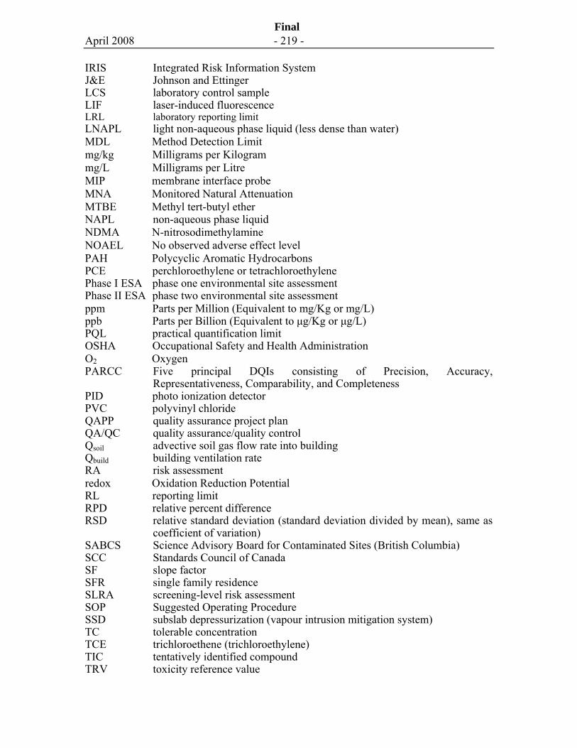
April 2008 - 219 -

Final

IRIS Integrated Risk Information System J&E Johnson and Ettinger LCS laboratory control sample LIF laser-induced fluorescence LRL laboratory reporting limit LNAPL light non-aqueous phase liquid (less dense than water) MDL Method Detection Limit mg/kg Milligrams per Kilogram mg/L Milligrams per Litre MIP membrane interface probe MNA Monitored Natural Attenuation MTBE Methyl tert-butyl ether NAPL non-aqueous phase liquid NDMA N-nitrosodimethylamine NOAEL No observed adverse effect level PAH Polycyclic Aromatic Hydrocarbons PCE perchloroethylene or tetrachloroethylene Phase I ESA phase one environmental site assessment Phase II ESA phase two environmental site assessment ppm Parts per Million (Equivalent to mg/Kg or mg/L) ppb Parts per Billion (Equivalent to μg/Kg or μg/L) PQL practical quantification limit OSHA Occupational Safety and Health Administration O2 Oxygen PARCC Five principal DQIs consisting of Precision, Accuracy,

Representativeness, Comparability, and Completeness PID photo ionization detector PVC polyvinyl chloride QAPP quality assurance project plan QA/QC quality assurance/quality control Qsoil advective soil gas flow rate into building Qbuild building ventilation rate RA risk assessment redox Oxidation Reduction Potential RL reporting limit RPD relative percent difference RSD relative standard deviation (standard deviation divided by mean), same as

coefficient of variation) SABCS Science Advisory Board for Contaminated Sites (British Columbia) SCC Standards Council of Canada SF slope factor SFR single family residence SLRA screening-level risk assessment SOP Suggested Operating Procedure SSD subslab depressurization (vapour intrusion mitigation system) TC tolerable concentration TCE trichloroethene (trichloroethylene) TIC tentatively identified compound TRV toxicity reference value

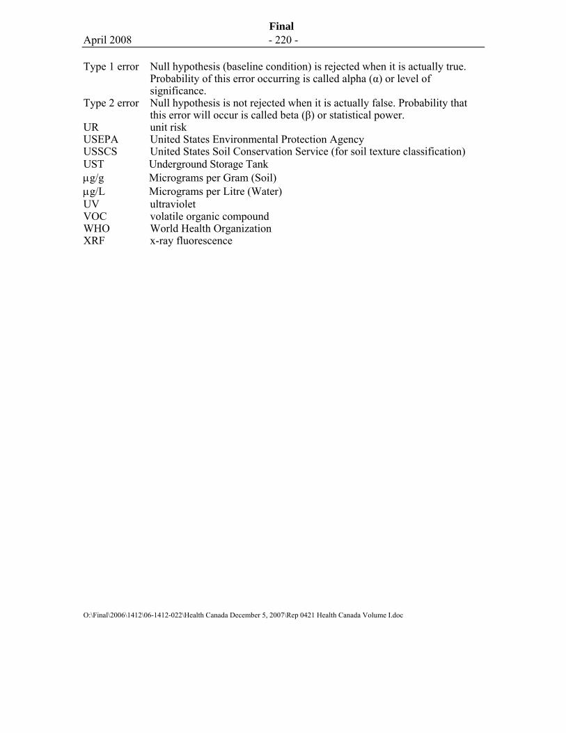
April 2008 - 220 -

Final

Type 1 error Null hypothesis (baseline condition) is rejected when it is actually true. Probability of this error occurring is called alpha (α) or level of significance.

Type 2 error Null hypothesis is not rejected when it is actually false. Probability that this error will occur is called beta (β) or statistical power.

UR unit risk USEPA United States Environmental Protection Agency USSCS United States Soil Conservation Service (for soil texture classification) UST Underground Storage Tank μg/g Micrograms per Gram (Soil) μg/L Micrograms per Litre (Water) UV ultraviolet VOC volatile organic compound WHO World Health Organization XRF x-ray fluorescence

O:\Final\2006\1412\06-1412-022\Health Canada December 5, 2007\Rep 0421 Health Canada Volume I.doc