Scottish Natural Heritage

Guidance noteAssessing collision risk between underwater turbines and marine wildlife

Version 1May 2016

i

CONTENTS

1 Introduction

2 Models for collision risk assessment

2.1 Encounter Rate Model

2.2 Collision Risk Model

2.3 Exposure Time Population Model

Further considerations for collision risk modelling

2.4 Avoidance, attraction and mortality

2.5 List of parameters required

2.6 Choosing which model to use

2.7 Impact on species populations

3 Obtaining animal density from survey data

3.1 Obtaining information on animal abundance

Vantage point survey

Boat-based survey

Digital aerial survey

Seal usage maps

SCANS – II Cetacean survey

European Seabirds at Sea database

Telemetry

Passive Acoustic Monitoring

Abundance estimates

3.2 Deriving animal density from survey data

Distance correction

Allocating unidentified species

Adjustment for nocturnal activity

Correcting for proportion underwater or airborne

Correcting for watch time

4 Density of animals at collision risk depth

4.1 Calculating the volume density

4.2 Estimating the proportion of animals at risk depth

4.3 Use of data on proportion of time at different depths

4.4 Use of dive behaviour models

4.5 Overall dive frequency

4.6 Mean time per dive at collision risk depth

5 Guidance on using the Underwater Collision Risk spreadsheet

5.1 Introduction to the spreadsheet

ii

5.2 Colour coding

5.3 Spreadsheet protection

5.4 Spreadsheet extension

5.5 Density (birds) worksheet

5.6 Density (marine animals) worksheet

5.7 ERM Worksheet

5.8 CRM Worksheet

5.9 ETPM Worksheet

5.10 Dynamic linkage

6 Cumulative assessment

7 Other turbine types

8 Recommended parameter values (eg animal sizes/ swim speeds)

8.1 Marine animals

Harbour porpoise

Harbour seal

Grey seal

Minke whale

Basking shark

Atlantic salmon

8.2 Diving birds

8.3 Avoidance rates

9 References

10 Worked examples

WE1: Fall of Warness, Orkney – marine animals

WE2: Fall of Warness, Orkney – diving birds

WE3: Pentland Firth – European shag

WE4: Pentland Firth – Atlantic salmon

This guidance note should be cited as:

Scottish Natural Heritage (2016) ‘Assessing collision risk between underwater turbines and marine

wildlife’. SNH guidance note.

This guidance note is written by Bill Band.

1

SECTION 1: INTRODUCTION

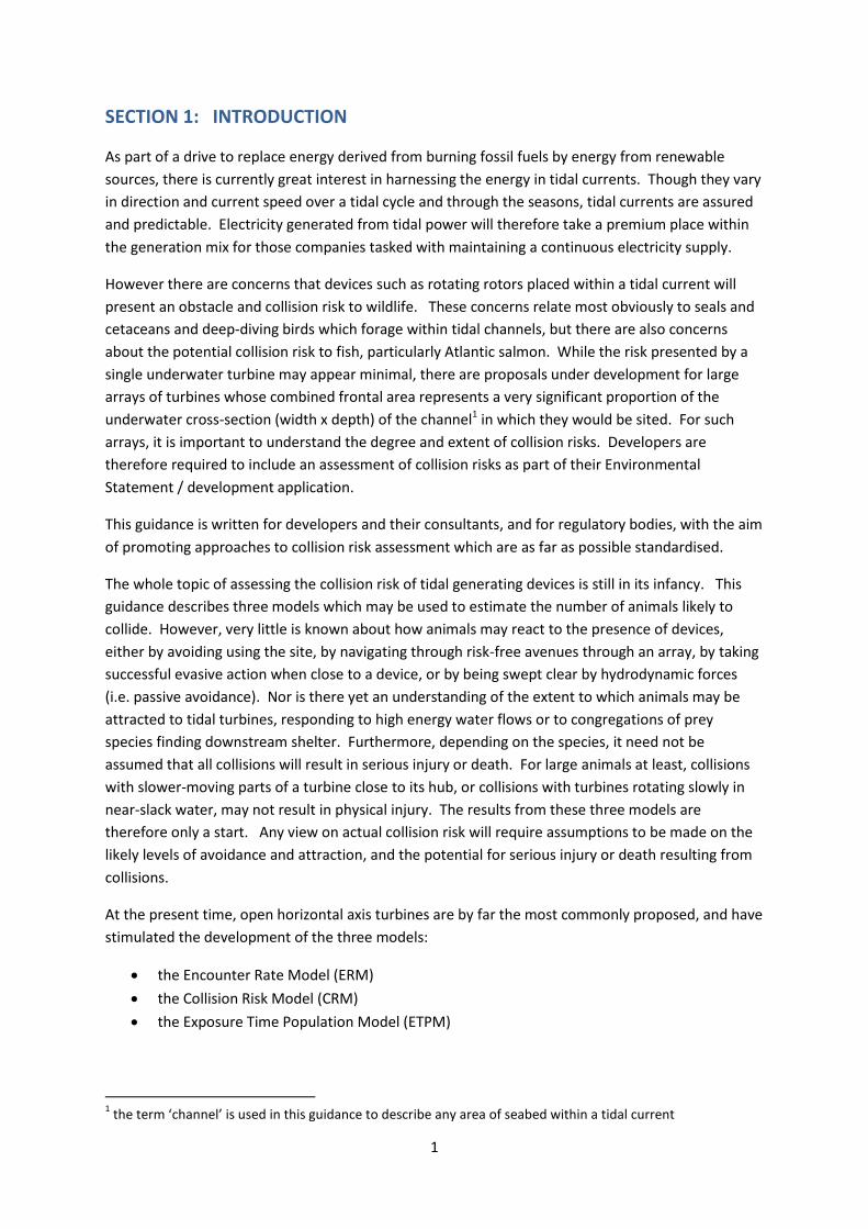
As part of a drive to replace energy derived from burning fossil fuels by energy from renewable

sources, there is currently great interest in harnessing the energy in tidal currents. Though they vary

in direction and current speed over a tidal cycle and through the seasons, tidal currents are assured

and predictable. Electricity generated from tidal power will therefore take a premium place within

the generation mix for those companies tasked with maintaining a continuous electricity supply.

However there are concerns that devices such as rotating rotors placed within a tidal current will

present an obstacle and collision risk to wildlife. These concerns relate most obviously to seals and

cetaceans and deep-diving birds which forage within tidal channels, but there are also concerns

about the potential collision risk to fish, particularly Atlantic salmon. While the risk presented by a

single underwater turbine may appear minimal, there are proposals under development for large

arrays of turbines whose combined frontal area represents a very significant proportion of the

underwater cross-section (width x depth) of the channel1 in which they would be sited. For such

arrays, it is important to understand the degree and extent of collision risks. Developers are

therefore required to include an assessment of collision risks as part of their Environmental

Statement / development application.

This guidance is written for developers and their consultants, and for regulatory bodies, with the aim

of promoting approaches to collision risk assessment which are as far as possible standardised.

The whole topic of assessing the collision risk of tidal generating devices is still in its infancy. This

guidance describes three models which may be used to estimate the number of animals likely to

collide. However, very little is known about how animals may react to the presence of devices,

either by avoiding using the site, by navigating through risk-free avenues through an array, by taking

successful evasive action when close to a device, or by being swept clear by hydrodynamic forces

(i.e. passive avoidance). Nor is there yet an understanding of the extent to which animals may be

attracted to tidal turbines, responding to high energy water flows or to congregations of prey

species finding downstream shelter. Furthermore, depending on the species, it need not be

assumed that all collisions will result in serious injury or death. For large animals at least, collisions

with slower-moving parts of a turbine close to its hub, or collisions with turbines rotating slowly in

near-slack water, may not result in physical injury. The results from these three models are

therefore only a start. Any view on actual collision risk will require assumptions to be made on the

likely levels of avoidance and attraction, and the potential for serious injury or death resulting from

collisions.

At the present time, open horizontal axis turbines are by far the most commonly proposed, and have

stimulated the development of the three models:

the Encounter Rate Model (ERM)

the Collision Risk Model (CRM)

the Exposure Time Population Model (ETPM)

1 the term ‘channel’ is used in this guidance to describe any area of seabed within a tidal current

2

The three models described in this guidance are basic and simple in concept, and may well be

refined over the course of time. They all address only one particular type of tidal generator – open

horizontal axis turbines, though Section 7 outlines how the ERM and CRM models may be adapted

for turbines consisting of an annular ring of blades, or for turbines with twin contra-rotating rotors.

The models are not suited to turbines contained within a cowl or tube, which may amplify current

speeds and affect animal swim direction; and in particular they are inappropriate for generators

installed within a tidal barrage.

The approaches of the ERM and CRM are broadly similar in that they both use a physical model of

the rotor and the body size and swimming activity of the animal to estimate the potential collision

rate. The ERM model focuses on the volume per unit time swept by each blade, while the CRM

focuses on the number of animal transits through a rotating rotor and the collision risk during each

transit. In both models, the shape of the rotor blades and animal are highly simplified, and single

mean values are used for tidal current, animal and rotor speeds. Nonetheless the results give a

reasonable indication of the likely level of risk in the absence of avoidance. For both models, as

described in section 2.4, there is a need then to consider the potential for animals to avoid the

turbines – which may lead to applying an appropriate avoidance rate; and to consider the likelihood

that a collision will cause death or serious injury to the animal. Finally there will be a need to view

such collision and mortality rates in the light of the dynamics of the animal population.

The ETPM uses population modelling to assess the critical additional mortality due to collisions

which would cause an adverse effect to an animal population. The model translates that into the

collision rate for each animal within the volume swept by the rotors which would be sufficient to

cause such an effect. It then calls for a qualitative judgement on whether such a collision rate is

likely. Though the ETPM model was developed to assess collision risks with diving birds, it could be

applied to other receptors if suitable population data are available.

Each of these models, and the equations used to make the necessary calculations, are outlined in

turn in sections 2.1-2.3. Section 2.4 describes the use of an avoidance factor to take account of

animals avoiding or evading collision risks. Section 2.5 lists the parameters required for each model,

Section 2.6 discusses which models are most appropriate for various circumstances, and Section 2.7

outlines how the outputs may be used to assess impacts on species populations. A spreadsheet

containing separate worksheets for each model accompanies this guidance and Section 5 contains

detailed guidance on its use.

The use of a spreadsheet makes it easy to calculate figures to several decimal places. It must be

remembered throughout that in the absence of a better understanding about animal behaviour in

the presence of underwater turbines, quantitative assessments of collision risk can at best provide a

rough pointer to the scale of these risks, and should be interpreted in the light of the major

outstanding uncertainties about animal behaviour, as well as the simplifications inherent in the

models.

Throughout this guidance, the word ‘animal’ includes both marine animals (including fish, cetaceans

and pinnipeds) and diving birds. An ‘encounter’ occurs whenever the trajectories of animals and

turbine blades are such as would lead to a collision, assuming no avoidance by the animal, whether

active or passive. The term ‘encounter rate’ (used in the ERM) is thus equivalent to the term ‘no-

avoidance collision rate’ (used in the CRM).

3

SECTION 2: MODELS FOR COLLISION RISK ASSESSMENT

2.1 The Encounter Rate Model

The Encounter Rate Model (ERM) was first described by Wilson et al (2007), and used to predict

potential encounters with marine mammals (harbour porpoise) and fish (herring), though the

authors envisaged the model could also be adapted and extended for diving birds. An ‘encounter’

occurs whenever the trajectories of animals and turbine blades are such as would lead to a collision,

assuming no avoidance action whatsoever is taken by the animal – either evasive action in the

vicinity of the rotors, or avoidance of use of the site by the animals, or simply being swept clear of

the blades by hydrodynamic forces. Based on a model previously used to estimate encounters

between marine predators and prey (Gerritsen & Strickler 1976), the ERM considers the volume

swept by each rotor blade (the ‘predator’) and the number of marine animals (the ‘prey’) present,

either wholly or partially, within that volume. Animals are assumed to be swimming in random

directions relative to the water body, and with random orientation, usually in the direction of their

swimming – this is an assumption of the predator-prey model which is not fully representative of

swim directions through a tidal channel. The resulting encounter rate is expressed in terms of the

number of animals per month or year which would encounter a turbine.

Imagine an object of cross-sectional area A swept with speed v through water containing D animals

per m3. In one second the object will sweep out a volume A v. All animals within that volume will be

‘encountered’ by the object in that one second, so

Number of encounters in one second = D A v (1)

The ERM is an application of this simple formula, with some refinements, to each blade of a turbine.

The cross-sectional area of a blade is basically its width w times its length R, except that allowance

must be made for the average clearance required r for the centre of an animal to pass the blade if it

is not to make contact because of its body width: this adds a distance r to the length of the blade

and a distance r at both sides of its width (see Figure 2). Thus:

effective cross-sectional area of each blade = (w+2r) (R+r) (2)

D

v A

Figure 1: animals encountered by an object

4

Figure 2: effective cross-sectional area of blade, allowing for average required clearance r

Note that the blade width w used here is the width of the blade from front to back, as viewed from

the side, not as viewed from the front2.

The cross-sectional area of a single blade is then multiplied by the number of blades b, and by the

number of rotors B if the assessment is for an array of turbines.

If the animals are also moving relative to the water, with a mean swim speed u, then the speed v

must be refined to take account of that swim speed, averaging over all possible directions (given the

assumption of random directions). When the blade speed is greater than the swim speed, which is

usually the case, factor v in equation (1) becomes

v ( 1 + (u2/3v2) ) (3)

This reduces to v if the swim speed is zero. For the derivation of this factor, see Wilson et al. (2007).

The blade speed v relative to the water is itself the result of combining the mean speed of the blade

relative to the hub vr , taken as the speed of the midpoint of the blade, and the speed of the water

relative to the hub, i.e. the current speed vc. As the current speed is perpendicular to the tangential

movement of the blades,

v =√ ( vr2 + vc

2) (4)

2 More strictly one should take an average of the cross-sectional area as viewed from all directions of closing

speed between blade and animal. However that would require detailed knowledge of blade shape. As blade speed usually exceeds animal speed, the great majority of collision trajectories will be nearly tangential with respect to the rotor axis, hence a side view predominates.

blade width w

clearance r

w + 2r

R + r

axis

rotor side view rotor front view

width w

blade length R

effective cross-sectional area of blade

(w+2r) x (R+r)

5

animal density

Thus the encounter rate per second developed from equation (1) is:

CERM = D x Bb (w+2r) (R+r) x v ( 1 + (u2/3v2) ) (5)

D is the ‘prey animal’ density, per m3

B is number of rotors

b is no of blades

w is the width of a turbine blade, as viewed from the side

R is the length of a turbine blade

r is the ‘effective radius’ – the clearance required due to the body size of the prey animal

v is the blade speed relative to the water, combining tangential speed and current speed

u is the prey animal’s swim speed relative to the water

A key parameter in the ERM is the ‘effective radius’ r of the animal at risk. Take L as the largest

dimension of the animal. If the animals were spherical in shape, the clearance required to avoid an

approaching blade would be L/2, if L is the diameter. If the centre of the animal comes closer than

L/2 to an approaching blade, then it will encounter the blade.

However for a stick-like animal – long and thin - the clearance required depends on the animal’s

swim orientation. If the orientation is perpendicular to the direction of approach of the blade, then

again the clearance required will be L/2, half the long dimension. But if it swims in alignment with

the direction of blade approach, the clearance required will be small, approaching zero if it is very

thin. For an infinitely thin animal, taking an average over all possible orientations, and assuming the

orientation is at random, gives an average clearance required of 0.5 (L/2) (see Bailey & Batty 1983,

describing the effective radius within which prey animals will encounter a predator; and Band,

2012b3).

Other shapes of animal are intermediate. An animal which approximates to a flat disc of diameter L,

also with random orientation, would require clearance on average of approximately 0.8 (L/2) (Band

2014). The clearance required is termed the ‘effective radius’ r of the animal and is related to the

longest dimension via a ‘shape factor’ f:

effective radius = f x L /2 (6 )

To date, fish, marine mammals and diving birds which use their feet to propel themselves

underwater have been modelled as long stick-like animals, while diving birds which use their wings

to scull underwater have been modelled as flat disc-shaped animals. Any departure from that

practice should be agreed with the regulator and statutory nature conservation bodies (SNCBs).

3 Note that the shape factor in Band 2014 is 2/f where f is as presented here

cross-sectional area of B rotors each with b blades

mean speed of blade relative to animal

6

Table 1: shape factors recommended for use with ERM

animal type model shape of animal

shape factor f

spherical 1

wing-propelled diving birds flat disc-shaped 0.8

fish, sea mammals, foot-propelled diving birds

long and thin 0.5

CERM is the encounter rate and must be multiplied by the time operating in a given period, to yield an

estimate of the number of encounters in that period. Tidal turbines do not operate in slack water,

so there is a proportion of time that turbines may be expected to be non-operational, in addition to

any periods required for maintenance; then

Number of encounters in the period = CERM t (1-nop) (7 )

where t is the number of seconds in the period, and nop is the proportion of non-operational time

expected. To arrive at an estimate of the number of collisions resulting, this must finally be

multiplied by the non-avoidance factor – the proportion of animals failing to take effective

avoidance action – see section 2.4 and equation (20).

Figure 3 shows schematically how the results of applying the ERM model may be used to inform an

impact assessment. Table 2 on page 16 gives a full list of the input parameters required for the

ERM.

7

2.2 The Collision Risk Model

The Collision Risk Model (CRM) (Band 2000; Band et al. (2007; Band 2012a) is widely used to

estimate the risk to birds flying through wind farms, and is here modified to address underwater

collision risks with tidal turbines. It may be applied to marine animals and diving birds, although the

assumptions made on direction of approach are not very realistic for the latter.

The model considers the number of animals likely to pass through each rotor, and the probability of

collision for each such passage. The CRM refers to a ‘no-avoidance collision rate’, i.e. the collision

rate assuming no avoidance action – this is a concept equivalent to the ‘encounter rate’ in the ERM.

In the CRM the animals are assumed to be swimming in a direction directly towards the rotor, i.e. in

a direction perpendicular to the rotor plane. In the underwater context what this means is that any

component of animal speed in the vertical direction (i.e. dive speed for diving animals), or parallel to

the rotor, is ignored. Only the component of velocity directly towards the rotor, taken as the mean

current speed, is considered when calculating the risk of collision in one transit, though dive speed

affects the time an animal is at risk and hence the number of transits.

Animal parameters

Turbine parameters

Animal activity

Activity at rotor

depth

Collision risk model or

Encounter rate model

Figure 3: Schematic of process for ERM and CRM models

No-avoidance Collision

rate or Encounter rate

Avoidance/attraction

assumptions

Collision rate estimate

Is this level of injury or mortality

acceptable?

Population modelling

Injury/ mortality assumptions

Injury/mortality rate

8

The CRM calculates the number of passages through a rotor which would be made by animals during

a period such as a year, using the same formula as equation (1) above for the ERM but applying it to

complete rotors, not to each individual blade. However, given that there is a significant probability

of an animal passing through a rotor without colliding, this is then multiplied by the risk of collision

during a single transit:

Collision rate derived using the CRM model:

CCRM = D x B π (R+0.5W)2 x v x pcoll (8)

D is once again the animal density in animals m-3.

The cross-sectional area of each turbine through which animal transits may occur is π (R+0.5W)2

where the radius R is extended by half an animal breadth 0.5W to allow for animals not clearing the

blade tips4.

v is the speed with which the animals approach the rotors.

In one second, all animals within a cylindrical volume of cross-sectional area π (R+0.5W)2 and length

v (i.e. volume π (R+0.5W)2 v ) will pass through a rotor. Thus, for B rotors, the number of transits in

unit time is

No of transits = D B π (R + 0.5W)2 v where D is animal density, in animals/m3 (9)

Not all transits through the swept area of a rotor will lead to a collision, however, since there is

space for passage between the blades, at least for animals which are small relative to the turbine. In

a second stage, the CRM multiplies that transit rate by the average risk of collision for a single

transit, calculated using information on blade size, taper, speed of rotation, and on animal size,

shape and speed:

No of collisions = No of transits x Risk of collision during a single transit (10)

The idealised animal shape used in the model is as shown below, pictured as two solid cones, stuck

together base to base, travelling in a direction along its longitudinal axis. This shape is quite well

matched to the shape of a marine mammal, if the circular cross-section at the widest point is

regarded as the body cross-section, at its widest point, of a marine mammal.

4 This adjustment from R to R+0.5W has not normally been applied when considering bird collisions with wind

turbines where W≪R. The adjustment is potentially much more significant for large marine animals and tidal turbines.

animal density cross-sectional

area of B rotors

animal speed mean risk of collision

during single transit

9

It is assumed that the animals are diving vertically through the risk zone, such that their velocity

component parallel to the rotor axis is just that from the current speed. This is likely to be a gross

simplification: most animals dive at an angle to the vertical, and the time at risk depth may include

some time foraging (e.g. for seal V-dives). However, this simplification makes the calculation

manageable.

In the CRM each blade of the rotor is modelled as a twisted lamina, that is to say the blade has a

width (the ‘chord’) which typically has a maximum some way out from the centre, then tapers off to

become narrow at the tip (see Figure 5). The blade is assumed to have no thickness (though in

reality it will have an aerofoil cross-section). If c is the chord width at radius r, and C is the

maximum chord width, the blade chord profile is expressed as a set of values for c/C for values of r/R

from 0 to 1. The pitch of the blade – the angle between the flat of the blade and the rotor plane – is

usually quite small (say 5 degrees) near the tip but increases towards the centre.

Figure 5: Model blade shape showing how blade chord width and pitch vary with radius

Figure 4: Idealised shape of an animal (red dotted lines) used in CRM

max chord

C

current

vc

rotor

rotor axis

blade

pitch γ(r) increases

towards centre

radius R

10

The risk of collision during a single transit at radius r from the centre can be calculated geometrically:

p(r) = (bΩ/2πv) [ |c sin γ + α c cos γ| + max (L, Wα) ] (11)

where

r is the radius from the rotor centre at the point of transit

b is no of blades

Ω is rotational speed

v is speed of animal relative to rotor (taken as the mean current speed)

c is the chord width of the blade at radius r

γ is the pitch angle of the blade at radius r, relative to the rotor plane

L is the length of the animal

W is its breadth (wingspan for a bird)

α = v/rΩ

For the derivation of equation (11) see Band et al. (2007) or Band (2012). It is sufficient to note here

that the collision probability p(r) depends on rotor rotation speed Ω, on both the frontal width of the

blades (c cos γ) and their depth (c sin γ) and on the dimensions (L, W) of the animal. The risk of

collision p(r) also depends on whether the transit is upstream or downstream: the + sign in the c sin

γ term refers to upstream passage; the – sign to downstream. The majority of transits will be

downstream, swept by the current, so the negative sign option in equation (11) is used hereafter in

this guidance.

When averaged over the rotor disk area, this gives a mean risk of collision pcoll for a single transit at

any random point in the rotor:

area of rotor disc area of rotor disc

pcoll = ∫∫ p(r) dA / ∫∫ dA (12)

where the integrations are over the area of the rotor disc: ∫∫ dA is just the area of the rotor πR2 .

The model assumes that the blades extend right to the rotor axis, i.e. there is no hub.

With this value calculated for pcoll, equation (8) can now be evaluated to get the collision rate CCRM. As with the ERM model, CCRM must be multiplied by the time in the period t, and the proportion of time operational, to get the number of no-avoidance collisions

CCRM t (1 – nop) (13)

where nop is the proportion of non-operational time expected. Finally it must be multiplied by a

non-avoidance factor – the estimated proportion of animals failing to take effective avoidance action

– to arrive at an estimate of the number of collisions resulting – see section 2.4 and equation 20.

The above equations describe the basic CRM model. If detailed data are available on the animal

depth distribution, a more refined approach may be used in which the density variation with depth

is taken into account alongside the variation in risk across the rotor. The data on the animal depth

distribution must be sufficient to describe the variation in animal density at depths between rotor

11

minimum and maximum depths. If the animal density at depth y is D(y) animals/m3 then equation

(8) becomes

CCRM = BπR2 x v x ∫∫ D(y) p(r) dA / ∫∫ dA (14)

Again the integrations are over the area of a rotor. The integration may be calculated numerically.

This is known as the extended CRM model; for species whose depth distribution is strongly skewed

towards the surface it may lead to a reduced estimate of collision risk.

As before CCRM must be multiplied by the time in the period t, and the proportion of time operational

nop , to get the number of no-avoidance collisions CCRM t (1 – nop).

Table 2 on page 16 lists the input parameters required to run the CRM model. The process by which

the CRM may inform an impact assessments is similar that for the ERM as described by Figure 3.

2.3 Exposure Time Population Model

The Exposure Time Population Model (ETPM) was developed by Grant, Trinder & Harding (2014) to

assess the collision risk to diving birds. In principle it could also be applied to assess collision risks

with marine animals, if adequate information on the population at risk were available.

The ETPM does not aim to provide a quantitative collision rate estimate like the previous two

models. Given the current lack of information on and understanding of animal responses to

turbines, the ETPM aims to present information about risk in a way which avoids making

assumptions on avoidance. It therefore starts at the other end of the process, using population

modelling to assess the critical additional mortality due to collisions which would cause an adverse

effect to an identified animal population. Knowing the number of animals in the population, and the

proportion of time each animal spends within the development site, it calculates the time for which

each animal in the population is exposed to risk – defined as the time, in the absence of any avoiding

action, within which each animal is likely to be found within the cylindrical volumes of water swept

by rotors. The model then combines these to estimate that collision rate for each animal within the

rotor-swept volume which would be sufficient to cause an adverse effect on the identified

population. It then calls for a qualitative judgement on whether such a collision rate is likely or not.

The basic equation for collision rate in the model is

t is the time period under study

CETPM is the collision rate, in collisions per second, during that time period 5

5 CETPM is used here rather than D as used in the source document, to avoid confusion with density D, and it is expressed as

a rate rather than total collisions during the period, to facilitate comparison with CCRM.

CETPM = N x T x α / t (15)

Collision rate

(per sec)

(secs)

No of animals

in population

time each individual

animal is exposed to

risk

collision rate for one

animal when exposed to

risk

time (secs)

in period

12

N is the number of animals in the population at issue, for example the animals within a

particular breeding colony.

T is the ‘exposure time’, i.e. the total time within the period for which each animal is exposed to

risk (i.e. the time it spends within the volume swept by rotors), assuming no avoidance

α is the collision rate – the number of collisions per unit time - for each animal exposed to risk

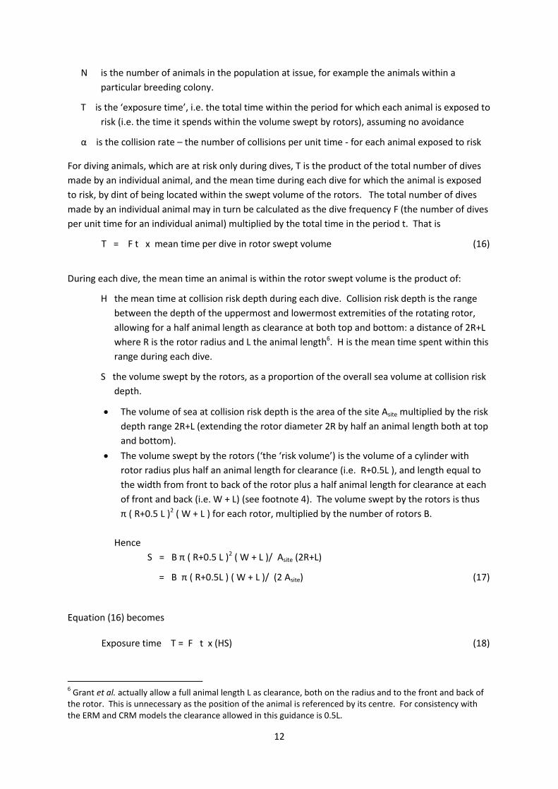
For diving animals, which are at risk only during dives, T is the product of the total number of dives

made by an individual animal, and the mean time during each dive for which the animal is exposed

to risk, by dint of being located within the swept volume of the rotors. The total number of dives

made by an individual animal may in turn be calculated as the dive frequency F (the number of dives

per unit time for an individual animal) multiplied by the total time in the period t. That is

T = F t x mean time per dive in rotor swept volume (16)

During each dive, the mean time an animal is within the rotor swept volume is the product of:

H the mean time at collision risk depth during each dive. Collision risk depth is the range

between the depth of the uppermost and lowermost extremities of the rotating rotor,

allowing for a half animal length as clearance at both top and bottom: a distance of 2R+L

where R is the rotor radius and L the animal length6. H is the mean time spent within this

range during each dive.

S the volume swept by the rotors, as a proportion of the overall sea volume at collision risk

depth.

The volume of sea at collision risk depth is the area of the site Asite multiplied by the risk

depth range 2R+L (extending the rotor diameter 2R by half an animal length both at top

and bottom).

The volume swept by the rotors (‘the ‘risk volume’) is the volume of a cylinder with

rotor radius plus half an animal length for clearance (i.e. R+0.5L ), and length equal to

the width from front to back of the rotor plus a half animal length for clearance at each

of front and back (i.e. W + L) (see footnote 4). The volume swept by the rotors is thus

π ( R+0.5 L )2 ( W + L ) for each rotor, multiplied by the number of rotors B.

Hence

S = B π ( R+0.5 L )2 ( W + L )/ Asite (2R+L)

= B π ( R+0.5L ) ( W + L )/ (2 Asite) (17)

Equation (16) becomes

Exposure time T = F t x (HS) (18)

6 Grant et al. actually allow a full animal length L as clearance, both on the radius and to the front and back of

the rotor. This is unnecessary as the position of the animal is referenced by its centre. For consistency with the ERM and CRM models the clearance allowed in this guidance is 0.5L.

13

Section 4.3 (page 31) describes two ways of calculating the overall dive frequency F, including the

method used by Grant et al.

The exposure time T may be calculated separately for different periods, eg for each month, or for

different seasons (eg breeding and non-breeding, for diving birds), and summed to yield an annual

exposure time.

There is no formula for calculating α from turbine and animal parameters, because the ETPM

method takes a rather different approach from that of the ERM and CRM. Both the ERM and the

CRM use a collision model to calculate the risk to animals within the risk volume, then apply an

assumed avoidance rate, so as to estimate collision rate: the question is then asked, does this

collision rate represent a significant adverse impact? The ETPM method takes a reverse approach,

using population modelling so as to identify the maximum additional mortality n in the time period t

(usually a year) which could be accepted without significant adverse impact on the population.

Equation (15) is then used in reverse to translate this maximum acceptable mortality into the critical

collision rate α for each animal, within the risk volume, which would inflict that level of mortality.

Having established values for N and T in equation (15), and noting that the total acceptable number

of collisions in the period is n = CETPM t, equation (15) can be turned round to

α = n / N T (19)

α is the collision rate for each animal, during the time it spends within the volume swept by rotors,

which would result in the maximum acceptable mortality (assuming all collisions were fatal).

The ETPM then asks the question, is such a collision rate likely, having regard for the likelihood of

high levels of avoidance?

Answering such a question is not straightforward. The collision rate for a single animal which, if it

took no avoiding action, would be within the rotor swept volume depends not just on the actual risk

from the rotor blades and their rotation speed, but also on the speed of the animal. The collision

rate also depends on the proportion of animals avoiding that risk by the various avoidance

mechanisms. Since α is derived directly from the maximum acceptable mortality, it is the critical

collision rate after allowing for possible safe passage through the rotors and likely levels of

avoidance. Although the ETPM does not include reference to assumptions on avoidance rates, the

proportion of animals taking avoiding action is implicit in the judgement to be made on the

likelihood of collision rate α being attained.

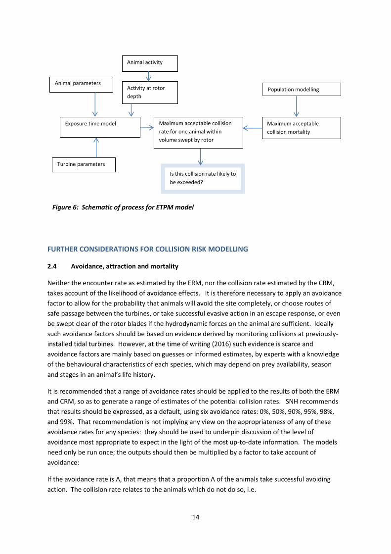
Figure 6 shows schematically how the ETPM aims to inform an impact assessment. Table 2 on

page 16 shows the input parameters required to run the Exposure Time component of the EPTM.

Population modelling requires detailed inputs on the population structure and breeding success, and

is outwith the scope of this guidance.

14

FURTHER CONSIDERATIONS FOR COLLISION RISK MODELLING

2.4 Avoidance, attraction and mortality

Neither the encounter rate as estimated by the ERM, nor the collision rate estimated by the CRM,

takes account of the likelihood of avoidance effects. It is therefore necessary to apply an avoidance

factor to allow for the probability that animals will avoid the site completely, or choose routes of

safe passage between the turbines, or take successful evasive action in an escape response, or even

be swept clear of the rotor blades if the hydrodynamic forces on the animal are sufficient. Ideally

such avoidance factors should be based on evidence derived by monitoring collisions at previously-

installed tidal turbines. However, at the time of writing (2016) such evidence is scarce and

avoidance factors are mainly based on guesses or informed estimates, by experts with a knowledge

of the behavioural characteristics of each species, which may depend on prey availability, season

and stages in an animal’s life history.

It is recommended that a range of avoidance rates should be applied to the results of both the ERM

and CRM, so as to generate a range of estimates of the potential collision rates. SNH recommends

that results should be expressed, as a default, using six avoidance rates: 0%, 50%, 90%, 95%, 98%,

and 99%. That recommendation is not implying any view on the appropriateness of any of these

avoidance rates for any species: they should be used to underpin discussion of the level of

avoidance most appropriate to expect in the light of the most up-to-date information. The models

need only be run once; the outputs should then be multiplied by a factor to take account of

avoidance:

If the avoidance rate is A, that means that a proportion A of the animals take successful avoiding

action. The collision rate relates to the animals which do not do so, i.e.

Animal parameters

Turbine parameters

Animal activity

Activity at rotor

depth

Exposure time model

Population modelling

Maximum acceptable

collision mortality

Maximum acceptable collision

rate for one animal within

volume swept by rotor

Is this collision rate likely to

be exceeded?

Figure 6: Schematic of process for ETPM model

15

Collision rate (per second) = (1-A) CERM or (1-A) CCRM (20)

A may be expressed either as a percentage (e.g. 98%) or a fraction (e.g. 0.98). The complement A’ =

(1-A) is sometimes referred to as the ‘non-avoidance rate’.

Attraction effects include the possibility that animals may be attracted to the high energy flow of

water through the turbines, or that prey may congregate in the shelter provided by fixed turbine

supports, or that diving birds may be attracted by moving blades visible within the water column. At

this stage of understanding these are even less amenable to description by a numerical factor but

should be considered qualitatively in any collision assessment.

The ETPM model does not require use of an avoidance rate. However the model requires a

judgement upon whether α - the rate of collision for each animal within the rotor swept volume

which would ‘just’ result in adverse impact on the population – is likely to be attained. α is

dependent, alongside other factors like blade size and rotation speed, on rates of avoidance and on

any attraction effects. So although it is implicit in the judgement to be made, rather than explicit

within the quantified collision risk, the same uncertainty over rates of avoidance and attraction

effects is present in the ETPM as in the ERM and CRM models.

A related issue is that of the relationship between collisions and animal mortality. Not all contact

between rotor blades and an animal will be fatal. Contact with peripheral parts of animals, or low

speed collisions with the slow-moving central parts of a rotor, may involve no or minor injury only.

Thompson et al. (2014b) conducted trials exploring the damage to seal carcasses from a boat-

mounted simulated turbine blade, of proportions akin to the SeaGen device in Strangford Lough.

The authors concluded that many collisions with the more rounded and slower parts of a turbine are

unlikely to kill or seriously injure seals; fewer than one third of impacts are likely to be fatal.

One approach to take account of this is to include another ‘mortality’ factor, though such a simple

approach as this does not allow for risk being selective, if for example juvenile animals were more

prone to injury.

In the ETPM model, which is driven by the critical added mortality which would lead to adverse

effect on the population, the factor α becomes the mortality rate due to collisions within the volume

swept by rotors; both potential avoidance or attraction and potential survival from impacts should

be taken into account when judging whether α is likely to be exceeded or not.

16

2.5 List of parameters required for each model

Table 2: Input parameters required for each model

ERM CRM ETPM Period t time in period(s) Tide data vc tidal current speed channel depth Turbine data no of rotors 2R rotor diameter b no of blades w width of blade from front to back C max chord width of blade λ pitch angle of blade c/C blade profile λ tip speed ratio Ω mean rotational speed nop proportion of time non-operational minimum depth of rotor Animal numbers N population of animals number of animals observed on site site area DS observed animal density per m

2

critical additional mortality Animal data species name L animal length W body width (wingspan for bird) u0 animal swim speed relative to water u vertical swim speed u’ plunge speed (plunge diving birds only) swim style (diving birds only) Dive data G number of foraging trips in period U dives per foraging trip p2 proportion of time foraging F2 dive frequency while foraging tu mean time underwater during dive ts mean surface time tw watch period dive type

17

2.6 Choosing which model to use

None of the models have been extensively applied and as yet it is difficult to say which model

approaches provide most insight on likely collision rates. At present there is a lack of monitoring

information from operational turbines to inform collision risk assessments, but when that is

available it seems likely to provide most insight on the nature and extent of animal avoidance and

attraction, rather than on the validity of the models themselves.

The ERM and CRM models are similar in nature, in that they lead to a quantitative estimate of the

encounter rate (assuming no avoidance action), then apply a range of assumptions on avoidance

rate so as to lead to an estimate of likely collision rates. These collision rates then require

interpretation, using population models if appropriate, to determine whether the collision rates

represent a significant adverse impact or not – but that stage lies outwith the scope of the models.

The main limitations of the ERM lie in the simplified shape modelled for rotor blade and animal, and

for both ERM and CRM in the assumptions made on the directions and speed of travel of animals as

they pass through the turbines.

The ETPM uses a population model to estimate the critical added mortality which would have a

significant adverse impact, then translates that added mortality to a rate of collision for animals

exposed to risk which would be just sufficient to cause such an impact. A judgement must then be

made on whether such a collision rate is likely or not. However the model provides little help on

how to make such a judgement, taking account of both the risk presented by rotor blades and likely

avoidance behaviour. In the two worked examples described by Grant et al. (2014), one (for

European shag) concludes that more than one collision every 7-8 minutes within the rotor risk

volume would have an adverse impact on the population, and the authors judge that this collision

rate may well be attained. The other (for common guillemot) concludes that more than one collision

every 25-40 seconds would be required to have an adverse impact on the population, and the

authors judge that, taking account of the likelihood that there will be some evasion and avoidance

behaviour, such a collision rate is unlikely to occur, though it cannot be entirely discounted. As

these collision rates must take into account not only the risk presented by rotor blades but also any

avoidance behaviour, these are difficult qualitative judgements to be made on the likelihood of

attaining the calculated critical collision rates. However, they may be no harder than judging, in the

present state of knowledge, what avoidance rates are reasonable to apply in other models. An

ETPM appraisal may be very helpful in circumstances where there is so little understanding of likely

behavioural responses that a decision based only on qualitative considerations is necessary.

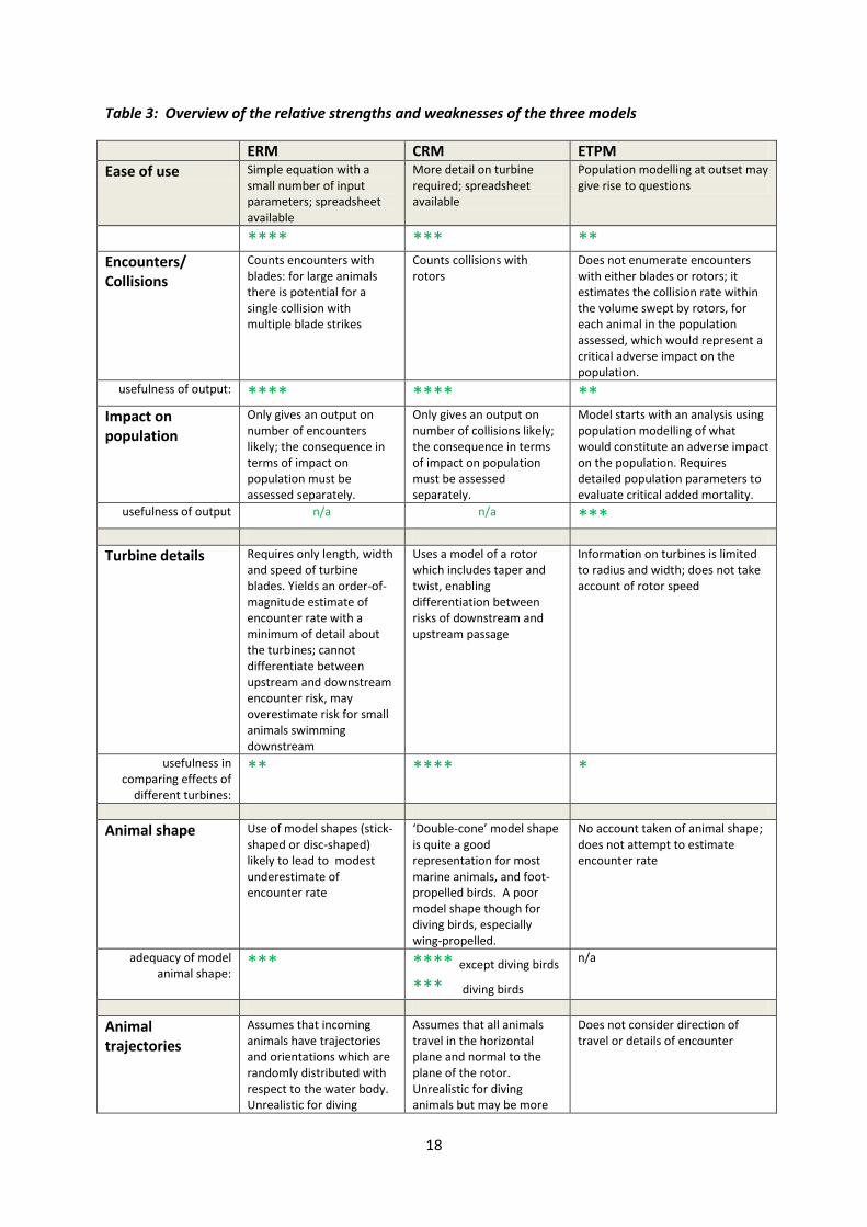
Table 3 on page 18 provides a provisional overview of the relative strengths of the three models7;

this table should be able to be refined once there is more experience on the application of the three

models. These notes are provided to help inform a decision as to which model should be used – or

whether, indeed, to use more than one model.

For some marine animals – notably fish species – data on the input parameters required for any

model may be so limited that only a qualitative or semi-quantitative assessment is possible. A

research strategy prepared for The Crown Estate, Marine Scotland and the Welsh Government

(ORJIP 2015) has pointed to the need for more evidence relating to collision risk and fish.

7 These are the views of the author of this guidance and not necessarily the views of SNH.

18

Table 3: Overview of the relative strengths and weaknesses of the three models

ERM CRM ETPM

Ease of use Simple equation with a small number of input parameters; spreadsheet available

More detail on turbine required; spreadsheet available

Population modelling at outset may give rise to questions

**** *** **

Encounters/ Collisions

Counts encounters with blades: for large animals there is potential for a single collision with multiple blade strikes

Counts collisions with rotors

Does not enumerate encounters with either blades or rotors; it estimates the collision rate within the volume swept by rotors, for each animal in the population assessed, which would represent a critical adverse impact on the population.

usefulness of output: **** **** ** Impact on population

Only gives an output on number of encounters likely; the consequence in terms of impact on population must be assessed separately.

Only gives an output on number of collisions likely; the consequence in terms of impact on population must be assessed separately.

Model starts with an analysis using population modelling of what would constitute an adverse impact on the population. Requires detailed population parameters to evaluate critical added mortality.

usefulness of output n/a n/a ***

Turbine details Requires only length, width and speed of turbine blades. Yields an order-of-magnitude estimate of encounter rate with a minimum of detail about the turbines; cannot differentiate between upstream and downstream encounter risk, may overestimate risk for small animals swimming downstream

Uses a model of a rotor which includes taper and twist, enabling differentiation between risks of downstream and upstream passage

Information on turbines is limited to radius and width; does not take account of rotor speed

usefulness in comparing effects of

different turbines:

** **** *

Animal shape Use of model shapes (stick-shaped or disc-shaped) likely to lead to modest underestimate of encounter rate

‘Double-cone’ model shape is quite a good representation for most marine animals, and foot-propelled birds. A poor model shape though for diving birds, especially wing-propelled.

No account taken of animal shape; does not attempt to estimate encounter rate

adequacy of model animal shape:

*** **** except diving birds

*** diving birds

n/a

Animal trajectories

Assumes that incoming animals have trajectories and orientations which are randomly distributed with respect to the water body. Unrealistic for diving

Assumes that all animals travel in the horizontal plane and normal to the plane of the rotor. Unrealistic for diving animals but may be more

Does not consider direction of travel or details of encounter

19

species with a preferred range of diving angles; may be more realistic for fish, though the majority of swim time may be broadly horizontal. Ignores hydrodynamic effects – the potential for animals to be swept clear of blades by the flow of water

realistic for some fish species. Assumes that all animals travel with a mean speed which is taken as the current velocity, which ignores the effect of swim speed. Ignores hydrodynamic effects – the potential for animals to be swept clear of blades by the flow of water

adequacy of model trajectories

*** ** except fish

**** fish

n/a

Choice of model to use will depend on the circumstances. Neither the ERM nor the CRM can be

regarded as an accurate calculator of encounter or collision rate. However both are likely to provide

a reasonable order-of-magnitude estimate. If the data are available, then both the ERM and CRM

may be used. It should be remembered that the assumptions on swim direction and orientation - in

the CRM that animals are passing through the rotor perpendicular to the rotor plane, and all with a

speed of the mean tidal current, and in the ERM that swim directions and orientation are at random

with respect to the water body - are often quite different from the real situation. Thus the results of

both should be regarded as ‘order of magnitude’ only.

For small animals – of size comparable with or less than the chord width of a turbine blade - the ERM

is likely to over-estimate encounter rate, as it does not take account of the geometry of the blade

and under-estimates the likelihood that a small animal moving downstream may pass between

blades, making use of the pitch of the blade to allow free passage.

The ERM counts encounters with blades, and for large animals this is likely to exceed the number of

encounters with rotors, since a large animal may experience multiple encounters with successive

blades. The time taken for an animal to swim past a rotor blade is L/v , while for a rotor with b

blades rotating at Ω/2π revolutions per second, the time between successive blade passes is 2π/bΩ.

When L/v > 2π/bΩ there is potential for an animal to encounter two or more blades in a single

transit through the rotor. However, if a high proportion of collisions are non-fatal, the number of

blade strikes may be just as relevant as the number of encounters with rotors in judging the

likelihood of death or serious injury.

The method as laid out in the ETPM of calculating dive frequency for diving birds is included in the

spreadsheet accompanying this guidance in the worksheet ‘Density (birds)’, and thus may be used to

calculate animal density when following the ERM or CRM analysis approaches as well.

It is recommended that the choice of model, and the reasoning behind that choice, should be

discussed and agreed with both the regulator and SNCBs in advance of presentation in the

application submission.

20

2.7 Impact of collisions on species population

Ultimately, the principal concern about collision risks is likely to be whether levels of injury or death

resulting from collisions will have an adverse effect on the species population. This may require

population modelling or a population viability analysis to understand the potential impact of the

additional mortality.

The ETPM begins with a population analysis developed for diving birds, leading to an estimate of the

critical additional mortality which would cause the affected population to decline. Both the ERM

and CRM only provide a view on potential collision rates. To interpret whether additional mortality

due to collisions would have an adverse effect on animal populations requires identification of the

population affected by the collision mortality, and potentially a population analysis akin to that

encompassed within the ETPM model.

Population modelling requires a sound body of data – on the size and bounds of the population, age

structure, and breeding success. Such a body of information may not be readily available for many

sites and species except for well-researched locations or after intensive survey effort. For fish

species, ICES8 data on fish populations used to inform the regulation of the fishing industry may be

helpful.

The Interim Population Consequences of Disturbance (PCoD) Framework 9 has been developed

primarily to investigate population effects of exposure to noise on marine mammals, mainly from

piling activity as a result of offshore wind farm construction. However it also has the facility to

model the additional effects of animals being removed from the population as a result of collision. It

can accept as an input the predicted number of collision related mortalities from a given project.

One of the benefits of the PCoD model framework is that it makes it possible to incorporate many of

the uncertainties in the input parameters into the predictions of effect. This means that the interim

PCoD framework provides a range of plausible values (i.e. with confidence intervals) as opposed to a

single best estimate. In the context of collision assessment, the uncertainty which could be

incorporated includes: uncertainty about the size of the population in a particular management unit;

uncertainty about the size of any vulnerable sub-population; uncertainty in the number of animals

that will collide with a particular development; uncertainty about the probability of death following

a collision, and the effects of demographic stochasticity and environmental variation 10.

8 International Council for the Exploration of the Seas http://www.ices.dk

9 http://www.scotland.gov.uk/Topics/marine/science/MSInteractive/Themes/pcod

10 with thanks to David Thompson, Sea Mammal Research Unit, for the text of this paragraph

21

SECTION 3: OBTAINING ANIMAL DENSITY FROM SURVEY DATA 3.1 Obtaining data on animal abundance

All three models require information on the number of animals present on the site – expressed in

the ERM and CRM models as areal density (animals m-2 or animals km-2) or in the ETPM model as the

number N in the population and the proportion P foraging on the site which is of area Asite. This

section outlines the main possible sources of information on animal abundance.

Detailed information on wildlife survey methodologies for marine sites can be found in the draft ‘Guidance on Survey and Monitoring in relation to Marine Renewables Deployments in Scotland’11, prepared for SNH and Marine Scotland by Royal Haskoning (2014) with input from a number of other environmental consultants.

There are three types of site characterisation survey which are most commonly used to obtain an

estimate of the abundance of marine wildlife activity in a tidal site:

(1) Survey from fixed vantage points on land,

(2) Boat-based survey, and

(3) Aerial survey.

Each of these is described in turn below. Different types of approach may be required for migratory

animals. Where possible, survey should aim to inform decisions on the siting of a development with

a view to minimising wildlife impacts.

Where local field survey information is not available for the development site, for example at an

early stage in planning a development, it may be helpful to make use of existing published sources of

animal abundance. Three important sources are:

(4) the Seal Usage Maps12, published by Marine Scotland,

(5) the SCANS – II cetacean survey, conducted in 2005 across European Atlantic waters, and

(6) the European Seabirds at Sea database (JNCC 2009), and the Atlas of seabird distribution in

north-west European waters (Stone et al 1995) founded on that data.

There are other forms of site monitoring which may also contribute to estimates of abundance:

(7) telemetry studies and (8) passive acoustic monitoring studies. While neither can provide good

information on abundance on its own, these can add to an understanding of abundance when

combined with other forms of survey.

Finally, where site survey information is not available, it may be possible nonetheless to make an

estimate of animal abundance from knowledge of population numbers elsewhere and applying

informed estimates on the extent of sea occupied. This may be the only practicable approach for

many fish species which are not amenable to visual survey methods. An example of such an

estimate being made is included as subsection (9) below.

11

http://www.snh.gov.uk/docs/B925810.pdf 12

http://www.gov.scot/Topics/marine/science/MSInteractive/Themes/seal-density

22

(1) Survey from fixed vantage points on land13

This type of survey involves a count of animals seen in the area of interest, from one or more fixed

vantage points. Typically the survey involves making a visual transect through the site, using

binoculars or telescope, and counting and recording animals seen at the sea surface. The scanned

area may be divided into zones, so as to identify animal counts within different parts of the site.

Correction is required for declining detectability of animals with distance. It cannot usually be

assumed however that animal abundance should remain uniform with distance, as there is often an

ecological gradient from coast to sea.

In the SNH and MS draft guidance on marine surveying and monitoring, it is advised that the scan

across the sea area should be as quick as possible so as to capture a snapshot of the animals present

at one point in time, i.e. quick enough that animals cannot redistribute; however the scan rate

should be slow enough that the chance of overlooking an animal is minimised. These two

requirements may not always be compatible. For cetaceans, seals and basking shark there is a

strong likelihood that animals may not be counted because they remain underwater during the time

that a given area of sea is watched. To allow for this, this guidance includes a correction for ‘watch

time’ i.e. the period of time during which any one part of the sea surface is watched during the scan.

Watch time is used in conjunction with the knowledge of dive and surfacing patterns to estimate the

proportion of animals unrecorded because they are underwater during the time that its location is

scanned. If the scan is performed as a continuous slow sweep, provided that a consistent scan rate

is maintained across the whole vantage point scan, the watch time tw may be calculated from the

rate of sweep and the field width of the binoculars/telescope:

Watch time (seconds) (t w) = Field width (degrees) / Scan rate (degrees per second) (21)

(2) Boat-based survey

Boat-based surveys are commonly used to provide data on abundance for diving birds and

cetaceans, and may also be used for seals. Observations are made from a boat following a sample

transect through the area of interest. An observer near the front records animals observed forward

of his/her position and within a prescribed range of observation to the side of the boat.

Observation protocols differ slightly as between these two species groups; for birds the method has

been standardised through the use of the European Seabirds at Sea protocol and is reviewed by

Camphuysen et al. (2004).

The method provides a count of animals visible within the transect strip. For unbiased results, it is

important that there is uniform effort coverage across the transect strip. Distance correction is

required, as visibility of animals in the further parts of the transect will be less than close to the boat.

13 Note that the vantage point watch methodology prescribed for use in gathering flight activity data at potential onshore

windfarm sites (SNH ) is not suitable for use in observing birds at sea or sea mammals. That technique involves scanning

the site to observe bird flight activity, and tracking and timing the duration of any flight. It is aimed at documenting the

activity of birds which spend a limited amount of time in flight and which are highly mobile.

23

To allow for animals which remain underwater during the period of observation of any one area of

sea, a watch time should be estimated and used in conjunction with knowledge of dive and surfacing

patterns, as for survey from fixed vantage points, to correct for this. If animals are counted within a

fixed distance forward of the boat, then

Watch time (seconds) (tw) = Distance observed forward of boat (m) / speed of boat (m s-1) (22)

(3) Digital aerial survey

Aerial survey involves flying over the site and taking high-quality digital aerial photographs or video

imagery from which the number of animals may be counted. This method gives a direct measure of

animal density on the sea surface. Distance correction is not necessary. Current techniques enable

distinguishing between birds in flight and birds on the sea, and have sufficient resolution to identify

a species group. Resolution to species level is often possible and is improving with improvements in

image analysis and analysis techniques.

Correction for animals underwater is required, using knowledge of diving and surfacing patterns for

each species. If digital still photography is used, the images are snapshots and watch time is

essentially zero. If video imagery is used, the watch time is the time taken to scan any one point on

the sea surface:

Watch time (seconds) = Transect length captured within image (m) / aircraft speed (m s-1) (23)

(4) Seal usage maps

These consist of two sets of maps, the first showing the areal density of grey seals and harbour seals

around the coast of Britain at a scale of 5km x 5km (Jones et al. 2015), and the second showing the

areal density of harbour seals around Orkney and the Pentland Firth at a finer scale of 0.6km x 0.6km

(Jones et al. 2016). Details of these are available from the Marine Scotland website14. The 5km x

5km maps show densities both for seals at sea, and for seals in total, including those hauled out.

The 0.6km x 0.6km maps show the densities for harbour seals at-sea. For the purpose of assessing

collision risks with underwater turbines, the ‘at sea’ maps should be used.

The maps have been compiled by the Sea Mammal Research Unit on the basis of a range of different

surveys, utilising both telemetry and field counts, over the period 1988-2015. The at-sea usage

maps are produced by looking at movement patterns from electronically tagged seals. The resulting

patterns of usage are scaled to population levels using data collected in aerial survey counts at haul

out sites, to produce estimates of mean density.

The figures mapped are mean seal counts and provide lower and upper 95% confidence bounds.

The figures must be adjusted to get the areal density of seals in animals/km2. Animals underwater

are already included and the figures do not require further correction for watch time.

14

http://www.gov.scot/Topics/marine/science/MSInteractive/Themes/seal-density

24

The maps use aggregated data from surveys during the period 1988-2015. While the data is biased

to an extent towards more recent surveys – because of their greater number and accuracy – it does

not represent a ‘current position’. Seal species may be subject to population trends which are not

revealed in these seal usage maps.

(5) SCANS – II Cetacean survey

This survey prepared a block-by-block estimate of small cetacean abundance in European Atlantic

waters, on the basis of a combination of boat-based and aerial surveys during 2005. The key species

reported on were harbour porpoise, white-beaked, bottlenose and common dolphin, and minke

whale. The figures provided are total abundance within each block, and thus must be divided by the

area of the block to get areal density in animals/km2. The survey methodology already allows for the

proportion of animals underwater and watch time effects.

(6) European Seabirds at Sea database

Background data on the abundance of seabirds in European waters is available from the European

Seabirds at Sea database, hosted by the JNCC (JNCC, 2009) and presented within ‘An Atlas of seabird

distribution in north-west European waters’ (Stone et al. 1995). This is a survey on a broad scale -

the atlas presents information in approximately 30kmx30 km squares – so it is unlikely that the

spatial scale of this data will be adequate for use in project-level collision assessments. However it

may be useful at the scoping stage of any assessment, providing a helpful baseline prior to any

detailed survey of the project site, and it will serve as a useful context for interpretation of survey

results.

(7) Telemetry

Telemetry is increasingly used to study marine animal populations, by tagging animals and

transmitting information back on location, depths and a variety of other factors either when the

animal surfaces, or when the tag is later retrieved. Tagging studies can provide a view on the spatial

distribution of a population – including in the depth dimension – but they cannot on their own

provide information on abundance. Where such data can be combined with separate information

on population number – for example, from counts of seals at seal haul-outs – then it can provide a

view of both distribution and abundance.

(8) Passive Acoustic Monitoring

Passive acoustic monitoring – using underwater microphones to detect the echolocation sounds

emitted by cetaceans – can also be helpful. However, there are difficulties in distinguishing between

species, and not every animal is actively echolocating , so the data must be used in conjunction with

visual (eg boat transect) surveys to yield good information on abundance.

(9) Abundance estimates

For some animals, such as migratory fish species, and in certain locations it will be impossible to

undertake site characterisation surveys and there will be no data sources available. In these

situations, and when collision risk assessment is required, it may be possible to estimate the

25

abundance by making a number of informed assumptions. For the MeyGen phase 1 Inner Sound

tidal array, for example, collision risk modelling was undertaken for Atlantic salmon (Xodus

Environment 2012). The assumptions made included numbers of returning adult Atlantic salmon

(making use of rod catch data and ICES population estimates), distribution across the width of the

Pentland Firth, and depth distribution. In such situations, and in order to agree any assumptions

made, it is recommended to engage in early dialogue with the Regulators and SNCBs.

3.2 Deriving animal density from survey data

The data acquired using any of the site characterisation survey methods requires some manipulation

in order to produce the best estimate of the total number of animals present on the sea or

underwater per unit area – the ‘areal density’ DA. Five stages of processing may be required, as

described below and summarised in Figure 7. The first three – distance correction, allocating

unidentified species, and adjusting for reduced night-time activity – lead to a refined estimate of DS,

the mean animal density observed at the sea surface. While these three adjustments are described

here, they are not included in the calculations within the model spreadsheets. The spreadsheets

require DS as a key input, following which the adjustments in the final two stages – correcting for the

proportion of animals underwater, and allowing for watch time – are included in the spreadsheets

and lead to an estimate of areal density DA, the mean animal density per square metre including

those underwater.

The process of correcting for the proportion underwater, and allowing for watch time, is often

termed ‘correcting for availability bias’ (i.e. an animal is only ‘available’ when it is observable within

the time it is being watched). Some surveys may also include distance correction within the scope of

correcting for availability bias. Care is therefore needed, when processing data from third party

surveys, to understand any availability corrections already applied to the data, so as not to duplicate

the corrections.

1. Distance correction

1. Distance correction 4. Correcting for proportion underwater

2. Allocating unidentified species

3. Adjustment for nocturnal activity

5. Allowing for watch time

DS mean animal density at surface

DA mean animal density including

those underwater

Raw survey data

Figure 7: Stages in processing survey data

26

Animals at a distance may not be observed because of poor visibility due to mist, precipitation or

wave or tide conditions. Distance correction aims to reverse such recording shortfalls by applying,

for each species, an appropriate distance-related multiplying factor. The assumption is made that

the actual density of animals is not dependent on distance, so that the animal density observed in

further-away segments should match that in close-by segments. DISTANCE software (see Buckland

et al. 2001) is often used to calculate the distance corrections required. More sophisticated analysis

may make use of the MRSea software package developed by Scott-Hayward et al. (2013) at CREEM.

In the context of surveying areas with potential for tidal turbines, care is needed to make this

underlying assumption only where it is unlikely that there will be spatial variation in habitats or tidal

conditions. In a survey from a vantage point, for example, it may be that the nearest segments

surveyed are coastal or shallow waters, while the furthest segments are deeper and strongly tidal.

In such a case it should not be assumed that animal densities for the near segments should match

those for further-away segments – the species mix may be very different.

However, when using boat-based survey at distances of 600m or more from shore on open coasts or

in wide channels, and where there is no evident cause for spatial variation in habitat, it may be

reasonable to assume that animal densities are uniform across the various distance bands, and that

any shortfall in observations is due to poorer visibility at distance.

2. Allocating unidentified species

There may be difficulty in identifying marine animals to species level. This is especially true in poor

weather or windy conditions when waves on the water may partially conceal animals, at the outer

reaches of a vantage point survey where distance makes identification difficult, and in aerial survey

when views of a bird from directly above are sometimes not adequate to identify it to species level.

However in many cases the observation may be confidently categorised in a species group.

Common species groups within which identification may be difficult are:

harbour seal and grey seal

dolphins and porpoise

whales

divers (red-throated, black-throated and great northern divers)

cormorant and shag

auks (guillemot, razorbill and puffin)

Sightings identified to species group but not to species level should be identified as such when

recording. Then these unidentified counts may be allocated to species in the same proportion as

those counts which are confidently identified to species level within the same survey. Thus, for

example, if 70% of identified seal counts were harbour seal, and 30% grey seal, then a count of 50

unidentified seals should be categorised as 35 harbour and 15 grey seal. Ideally the identified seal

counts used as the basis for such apportionment should be from the same survey area where the

unidentified seals were sighted, as the proportions of the two species are likely to vary with location

and according to habitat. If that is not possible, a second option is to choose areas as the basis for

apportionment which have similar habitat characteristics to where the non-identified seals were

27

sighted. Source areas used for apportionment should not be so restricted that statistical variance

could dominate the apportionment.

3. Adjusting for reduced activity at night

For obvious reasons observations, for all three types of survey, do not cover night-time periods.

Information on night-time activity of many marine species is very limited. A precautionary approach

is recommended, by assuming, unless there is evidence to the contrary, that marine species are

equally active at night as by day. Cormorant and shag are exceptions: it is well documented (Birdlife

International 2014) that these species do not normally forage by night.

Each species may be given a ‘nocturnal activity factor’ K to multiply the density as surveyed in

daytime. K=1 for those species just as active by night as by day. K=0 for species like cormorant and

shag which do not forage by night.

The effect of this adjustment is stronger in winter (when night hours are long) than in summer

(when night hours are short). Therefore the adjustment has to take into account the daytime and

night-time hours in each month:

Average density DS = Σ ( Di di + K Di ni ) / Σ ( di + ni ) (24)

where Di is the areal density in month i, and di and ni are respectively the daylight and night-time

hours in month i (the denominator is simply the total time across all 12 months). Forsythe

et al. (1995) set out a convenient means of calculating daylight and night hours, given the latitude of

the site.

If required, the analysis could be made more sophisticated by identifying different nocturnal activity

factors for different seasons (e.g. for diving birds, the breeding and non-breeding seasons), but this

is not done here.

4. Correcting for proportion underwater or airborne

Both for marine mammals and diving birds, the true areal density of animals present DA is not simply

that recorded by a snapshot observation at the surface, because at any instant of time a proportion

of the species concerned will be underwater. The position is most marked for some whales, which

may have a mean dive time over twenty times their mean surfacing period. If observations were a

snapshot of the surface, the areal density thus observed would have to be multiplied by over twenty

to give the areal density of animals in the sea. If DA is the areal density of animals in the sea i.e. on

or below the surface, then the density of animals observed on the surface in a snapshot count is

DS = DA x proportion of time visible at surface

or turning that around,

DA = DS / proportion of time visible at surface

Let the frequency of dives by any one animal be F dives/unit time (this is the overall frequency, the

time spanning rest periods on the sea surface as well as the periods occupied by diving bouts); and

the mean duration of a dive be tu . Then the number of dives per animal in time t (per animal) is F t

28

and their total duration F t tu. Hence the proportion of time spent underwater is F tu; it follows that

the proportion of time at the surface (and therefore visible) is ( 1 – F tu ). Putting this in the above

equation gives

True areal density DA = DS / ( 1 – F tu ) (25)

This is the correction required to take account of animals underwater for a snapshot count.

A similar correction is required for plunge-diving birds which spend a substantial proportion of time

airborne. If survey data represents the density of birds on the sea surface, then the true areal

density, including both airborne birds and those on the sea surface, is given by

DA = DS / ( 1 – proportion of time airborne) (26)

Worked Example WE2 (Section 10) illustrates the use of this correction for gannet.

5. Correcting for watch time

If the observation of an area of sea is not just a snapshot, but takes a significant length of time, then

animals may appear during that watch period while others may dive. The adjustment made to allow

for the proportion of animals underwater depends on the watch time – the period for which an area

of sea is watched. Normal survey practice is to record any animal visible at any time during the

period that each area of sea is watched.

If the observation of the area of sea is a lengthy one – longer than the dive cycle of the animal

concerned – then each animal will eventually surface and be observed; no correction for animals

underwater will be required. In contrast, still digital aerial photography provides digital photographs

which are genuine snapshots, with an exposure time lasting a small fraction of a second: correcting

for animals underwater as in equation (25) is required. Video aerial photography is analogous to a

manual transect using binoculars – equation (28) below should be used, allowing for the watch time

tw which is the time for the video to progress over any single complete field of view.

Consider a complete dive cycle for an animal, consisting of ts seconds visible at the surface followed

by tu seconds underwater. The time during which the animal may be spotted at the surface is ts + tw,

i.e. not just the duration of the surfacing but allowing for the watch period tw during which the

surfacing might commence. The full dive cycle lasts ts + tu seconds, so the proportion of time for

which the animal is observable is

( ts + tw ) / ( ts + tu )

which may be written as (ts + tu – tu + tw ) / (ts + tu ) or 1 – F (tu – tw)

where F is the overall dive frequency : F = 1/( ts + tu ) (27)

This must be modified if the watch period is greater than the duration of a complete dive cycle: the

proportion of time must reach a maximum value of 1, as the animal will be seen surfacing at some

time during the watch period:

Proportion of time animal is visible = 1 – F * max (0, tu – tw )

29

Thus DA = DS / [ 1 – F * max (0, tu – tw ) ] (28)

For watch periods longer than the dive period, this reduces to DA = DS, reflecting that there is no

need to adjust for animals underwater, as each animal will have surfaced and been counted during

the watch period.

If the watch period is very short (as in the snapshots taken by aerial photography), this reduces to

the expression for a snapshot, given in equation (25).

Table 4: Data processing stages required for different types of survey data

Survey type:

Vantage point Boat-based Digital aerial

1 Distance correction Yes Yes No

2 Allocation of unidentified species Yes Yes Yes

3 Adjustment for nocturnal activity Yes Yes Yes

4 Correcting for proportion underwater

Yes Yes Yes

5 Allowing for watch time Yes Yes No – watch time taken as zero (snapshot)

30

SECTION 4: DENSITY OF ANIMALS AT COLLISION RISK DEPTH

4.1 Calculating the volume density

In all three models, the collision rate is proportional to the volume density of animals in the water15,

the number of animals per m3, and an animal is only considered to be at risk of collision if it is at

‘collision risk depth’, meaning at a depth between the lowermost and uppermost rotor blade tips.

The preceding sections of this guidance describe how from survey data one may derive the areal

density of animals DA, that is the number of animals within each square metre (or square kilometre)

of water, whether on the surface or below. Assume a proportion Q2R swim at depths within the

collision risk depth range, a depth range of 2R in total if R is the radius of the rotor. Then the areal

density of animals swimming in this risk depth range is DAQ2R: that means there are DAQ2R animals in

a column of water 1m2 base and 2R high (see Figure 8). The mean density (by volume) within that

risk range water column is then the number of animals DAQ2R divided by the volume of the water

column at risk range, 2R m3. That is,

D = DAQ2R / 2R (29)

D is the true animal density, i.e. animals per m3

DA is the animal density measured in area terms, i.e. animals/m2 at any depth

Q2R is the proportion of animals within the range of depths at risk of collision, from the

greatest to the least depth of a rotor, i.e. twice the rotor radius

R is the rotor radius

Different turbines may occupy different depth ranges and hence Q2R is dependent on the turbine

and its diameter. The following section discusses how Q2R is estimated for different species.

DA and Q2R are the parameters used in the ERM and CRM models as described in this guidance. As

noted above, the ETPM does not refer to animal density but to the number of animals N in the

target population, the proportion P foraging on the development site, and the area of the

development site Asite; thus DA is equivalent to NP/Asite. The ETPM expresses the proportion at risk

depth in terms of the time H each animal spends at risk depth; this must be multiplied by the dive

frequency F to get the proportion of time at risk Q2R , as described below.

15

the ETPM does not use density as a parameter but refers to the animal population N using a given site area Asite, so the effect is the same; and expresses the proportion at risk in terms of H, the time an animal spends at collision risk depth, rather than Q2R.

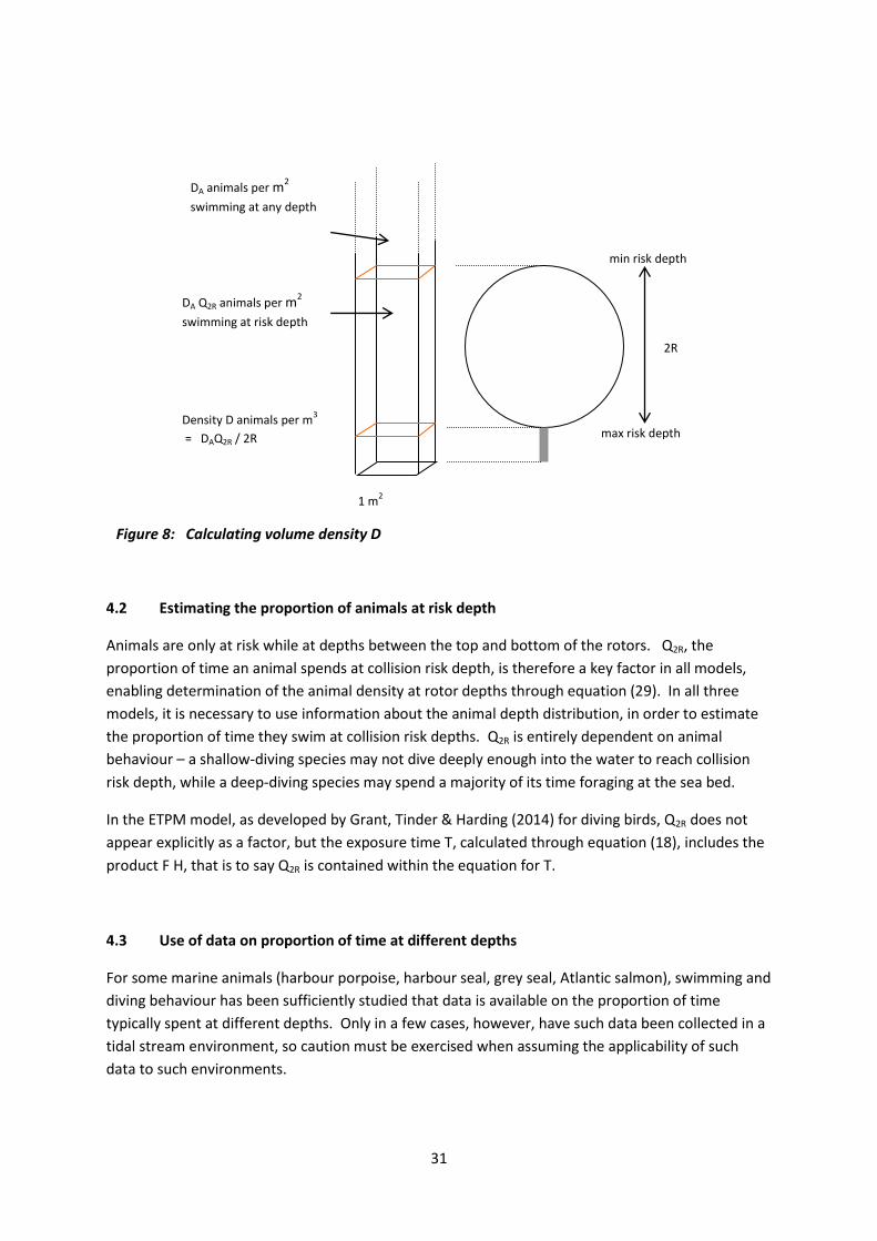
31

4.2 Estimating the proportion of animals at risk depth

Animals are only at risk while at depths between the top and bottom of the rotors. Q2R, the

proportion of time an animal spends at collision risk depth, is therefore a key factor in all models,

enabling determination of the animal density at rotor depths through equation (29). In all three

models, it is necessary to use information about the animal depth distribution, in order to estimate

the proportion of time they swim at collision risk depths. Q2R is entirely dependent on animal

behaviour – a shallow-diving species may not dive deeply enough into the water to reach collision

risk depth, while a deep-diving species may spend a majority of its time foraging at the sea bed.

In the ETPM model, as developed by Grant, Tinder & Harding (2014) for diving birds, Q2R does not

appear explicitly as a factor, but the exposure time T, calculated through equation (18), includes the

product F H, that is to say Q2R is contained within the equation for T.

4.3 Use of data on proportion of time at different depths

For some marine animals (harbour porpoise, harbour seal, grey seal, Atlantic salmon), swimming and

diving behaviour has been sufficiently studied that data is available on the proportion of time

typically spent at different depths. Only in a few cases, however, have such data been collected in a

tidal stream environment, so caution must be exercised when assuming the applicability of such

data to such environments.

2R

1 m2

DA animals per m2

swimming at any depth

DA Q2R animals per m2

swimming at risk depth

Density D animals per m3

= DAQ2R / 2R

min risk depth

max risk depth

Figure 8: Calculating volume density D

32

The proportion of time spent at different depths varies with the depth of the water, as much of the

foraging by some species is at or close to the sea bed, though some may be in mid-water column.

Depth data is presented in Section 8 for the above four species, and it is strongly recommended that

this be used where appropriate. The spreadsheet accompanying this guidance uses this data. Q2R is

calculated either by adding the proportions in each band within the collision risk depth range, or, if

the data is expressed on a cumulative basis, by subtracting the proportion swimming above

minimum depth from the proportion swimming above maximum depth.

4.4 Use of dive behaviour models

For many diving species, information on the proportion of time at different depths is simply not

available. However, the proportions may usually be estimated using one or other model of dive

behaviour.

Uniform distribution

The simplest model is to assume that the distribution of animals is uniform over the entire depth

range between seabed and surface. In this case the proportion of time at risk depth is simply that

proportion of water depth occupied by the diameter of the rotor:

Q2R = 2R / water depth (30)

where 2R is the range of collision risk depths, twice the radius R. This is a ‘default’ model,

recommended for use for basking shark for which detailed information on swim depth is not

available, but where it is known that they make use of the full water column. For other species for

which information is not available on their typical depth distribution, a precautionary approach may

be to assume a uniform distribution throughout the channel depth.

Deep diving, shallow diving and plunge diving:

Alternatively, if information is available on the speed of diving (while descending and ascending), Q2R

may be calculated by calculating the time during each dive the animal is at risk while swimming

down and back up through the range of risk depths, and multiplying by the frequency of dives:

Q2R = overall dive frequency (F) x mean time per dive at collision risk depth (H) (31)

The following two sections describe respectively how the overall dive frequency F, and the mean

time per dive at collision risk depth H, may be estimated. Note that neither of these parameters is

required if data are available directly on the proportion of time at different depths, as described in

section 4.3.

4.5 Overall dive frequency

A number of methods may be used to estimate overall dive frequency:

(a) For marine animals, if information is available on dive cycles and surfacing times, then the

overall dive frequency may be calculated as

33

F = 1/ (tu + ts) (32)

where tu is the mean dive time spent underwater, and ts the mean time at the sea surface. It is

important that these are means across all times, and are not just calculated from bouts of

foraging activity.

(b) For diving birds, if information is available about diving behaviour while foraging, the overall

dive frequency may be calculated as

F = dive frequency while foraging F2 x proportion of time on site spent foraging P2 (33)

Diving birds spend time on the sea surface resting and digesting, then have bouts of foraging in

which a series of dives are interspersed with a short rest period, e.g. to allow for re-

oxygenation. These diving bouts are well studied and thus data tends to be available on the

dive frequency while in foraging mode (F2) and on the duration of dives (tu). Also required,

though harder to find, is the proportion of time a bird spends foraging (P2). Only the time the

bird is at sea is counted: time away from the site should be excluded. The product F2P2 is then

the overall dive frequency. This is the ‘Method 1’ option in the spreadsheet.

(c) Alternatively for diving birds, overall dive frequency may be calculated on the basis of the

estimated number of foraging trips in the period for the species (G)16, and the mean number of

dives made per foraging trip (U):

F = GU/t = no of foraging trips in period x

no of dives per foraging trip / duration of period (34a)

This is the ‘Method 2’ option in the spreadsheet.

For the EPTM model, Grant et al. (2014) extend this to the situation where only a proportion P

of foraging trips made by each bird in the population are to the development site ; in this case

the equation becomes F = GUP/t. Note that this gives the overall dive frequency within the

development site for each bird from the population under assessment; it is the fraction P times

the overall dive frequency for each bird on site, and takes account of the fact that foraging trips

may be made to areas of sea within the bird’s foraging range other than the development site.

These formulae are most appropriate during the breeding season when foraging trips are

between sea and breeding colonies. Outwith the breeding season, birds may remain at sea

rather than return to their breeding colonies. In this case the calculation of overall dive

frequency for an individual bird may be modified to:

F = G’ U’ P’/ t (34b)

where G’ is the number of days in period, U’ the mean number of dives per day, and P’ the

mean proportion of birds from the colony population within the development site at any time.

(A conservative assumption might be that all birds from the colony forage in the development

site; and that birds from the colony are at sea for virtually 100% of the time; in such a case

P’=1.)

16

G is used here rather than F as used in Grant et al. (2014), to avoid confusion with the dive frequency F used here

34

In the accompanying spreadsheet, worksheet ‘Density (marine animals)’ enables the first of these

three methods to be used, while the worksheet ‘Density (birds)’ enables either of the last two

methods to be used. Figure 9 summarises the options available for estimating dive frequency:

4.6 Mean time per dive at collision risk depth

The assumption made here is that the proportion of time spent within the range of collision risk

depths depends on the vertical swim speed of the animal. Three models are suggested:

deep diving – this model assumes that animals dive in order to forage at the sea bed (i.e.

below collision risk depth); thus the ‘at risk’ times are only while passing through the risk

depth range during descent and ascent, and depend on the descent and ascent swim speeds

ud and ua . The ‘at risk’ time during each dive is

H = 2R/ud + 2R/ua (35)

and from equation (31) Q2R = F H where F is the dive frequency.

This model is suited to deep diving bird species like shag, cormorant, and black guillemot. A

simple mean of ascent/descent swim speeds u may be used, rather than separate descent and

ascent speeds, so that H = 4R/u.

shallow diving - this model is appropriate for animals which dive in order to forage within the

range of collision risk depth. During a dive, such an animal is not at risk only for the time it

takes to descend to, and ascend from, the level of the upper limit of the rotor blades hup. A

simple mean of ascent/descent swim speeds u may be used, rather than separate descent and

ascent speeds.

G = no of foraging trips

in period

P = proportion of trips

which are made to

development site

U = no of dives per

foraging trip

G’ = no of days in

period

P’ = proportion of birds

from colony within

development site

U’ = no of dives per day

breeding season non-breeding season

tu = mean time

underwater per dive

tu = mean time at

surface between

dives

F2 = frequency of dives

while foraging

P2 = proportion of time

spent foraging

F = 1 / ( tu + ts ) F = F2 P2

F = G’ P’ U’ / t F = G P U / t

(a) (b) (c)

Figure 9: Options for estimating

overall dive frequency

35

at risk time is H = tu – 2 * hup / u (36)

where tu is the dive duration

and hup is the upper limit of the risk range, i.e the minimum rotor depth

As before Q2R = F H where F is the dive frequency.

This model is best suited to shallow diving species like eider, red-throated diver and razorbill.

plunge diving – this model is appropriate for birds which plunge from the air to catch prey

then swim to the surface. This is similar to shallow diving except the descent uses a plunge

speed uplunge for the descent and a swim speed u for the ascent:

at risk time is H = tu – hup / uplunge – hup / u (37)

where tu is the dive duration

and hup is the upper limit of the risk range, i.e the minimum rotor depth

As before Q2R = FH where F is the dive frequency

This model has been applied to gannet in Worked Example 2 (Section 10).

Together with the ‘uniform distribution’ modelling summarised in equation (30), these three

approaches represent generic dive behaviours which may be used as appropriate to calculate Q2R for

different species groups. The four dive behaviour models are programmed in to the spreadsheet,

used by entering the ‘depth distribution type’ as ‘uniform’ (not available for birds), ‘shallow-diving’,

deep-diving’ or ‘plunge-diving’ (not available for marine animals).

Where the data is available, though, it is preferable to use a species-specific depth distribution to

enable calculation of Q2R. The spreadsheet currently contains four such distributions, initiated by

setting the ‘depth distribution type’ to ‘harbour porpoise’, ’ harbour seal’, ‘grey seal’ or ‘Atlantic

salmon’.

It is recommended that the dive behaviour models to be used in assessing collision risks should be

agreed with the Regulator and SNCBs prior to undertaking the assessment.

36

SECTION 5: GUIDANCE ON USING SPREADSHEETS 5.1 Introduction to the ERM/CRM/ETPM spreadsheet

To help in making use of the three models, the required calculations are set up within the

accompanying Excel spreadsheet. Within the spreadsheet, there are seven worksheets.

The first five worksheets are set out so that if the user feeds in the required input data (colour-coded

blue and green), the calculated results are then shown (colour-coded orange). For each of the

parameters listed in column A, help on that parameter is available by clicking on column B, in the

cells with red triangles at upper right. The symbol for the parameter as used in the guidance is listed

in column C, and the units used in column D. The values of the parameters are then input in column

E, or in later columns where the parameter differs according to species. For calculated fields,

column F shows the formula underlying the calculation. These formulae use the same symbols as in

the text, and are designed to show which part of the ‘master’ equations are being calculated in each

row.

The first two worksheets make an estimate of the animal density (diving birds and marine animals

respectively) at risk depth from survey observations of animals observed at the sea surface. These

two worksheets have a similar structure, but there are differences in the way that allowance is made

for time underwater (when animals are not visible), making it easier to use one worksheet for diving

birds, and the other for marine mammals and fish. The latter worksheet, for certain species, draws

upon data on depth distributions set out in the final worksheet ‘Swim depths’.

The third, fourth and fifth worksheets perform the necessary calculations for the ERM, CRM and

ETPM models respectively. The sixth worksheet – ‘Avoidance’ shows the results of applying various

assumed avoidance rates to the ERM and CRM predictions.

To use the ERM, start with the Density worksheet for Diving birds or Marine animals, as appropriate.

When the required data has been input to the Density sheet, copy the concluding figures for ‘Density

at risk depth’ into the ERM worksheet at row 21 (colour coded yellow). Now enter the remaining

data required in the blue fields of the ERM worksheet. The final line will then give the ‘encounter

rate per period’ which is the number of encounters (collisions) expected in the selected period (1

year), before any account is taken of avoidance.

To use the CRM, start with the Density worksheet for Birds or Marine animals, as for the ERM.

When the required data has been input to the Density sheet, copy the concluding figures for ‘Density

at risk depth’ into the CRM worksheet at row 35 (colour coded yellow). Enter the remaining data

required in the blue fields of the CRM worksheet. The ‘collision probability for single transit’ line

gives the mean risk of collision for each animal making a transit through the rotor. ‘No of rotor

transits in period’ gives the number of animals expected to transit through the rotor(s) in the

selected period (1 year). The final line ‘collisions in period before avoidance’ gives the expected

number of collisions in the period, before any account is taken of avoidance.

To use the ETPM, you don’t need the calculation of density at risk depth. However you do need the

calculation of the parameter Q2R which is the product of dive frequency F = GU/t and the mean time

at risk depth during a dive H. Use the appropriate Density sheet as before, though the bird densities

input in row 4 or 5 are not relevant and may be set to zero; the watch time too is not relevant and

37

may be set to zero. Once all the remaining input data has been entered, copy the values of Q2R (= F x

H) into row 25 of the ETPM worksheet. Also copy in the rotor diameter, from the Density worksheet

used. Now complete entry of data in the ETPM worksheet. The worksheet will now give the total

annual exposure time T per bird in the target population.

Calculation of the critical added mortality n will require a separate calculation using population

modelling techniques, outwith the scope of this guidance. Once the critical added mortality n is

entered, the worksheet computes the critical collision rate α which would have to be attained for

each bird in the target population if this critical level of added mortality were to be reached.

The remainder of this chapter describes the first five worksheets in detail. For each, following an

overview of the calculation sequence, a table is provided giving detailed guidance for each field.

The notes in these tables expand on the help text available within the spreadsheet by clicking on the

cells with the red triangles at upper right.

5.2 Colour coding

The cells in the spreadsheet have been colour coded to make it easy to see which cells are user

input, and which cells are fields calculated by the spreadsheet.

Blue fields are user input about the turbines. These will need review

whenever the calculation is applied eg to a different turbine or location.

Green fields are user input about the animals. These will need review

whenever information about the animal or its abundance is changed.

Pale orange fields are calculated by the spreadsheet, these are intermediate

workings.

Darker orange fields are final results, also calculated by the spreadsheet.

Yellow fields are data values copied from one of the Density sheets to the

CRM, ERM, or ETPM sheets

5.3 Spreadsheet protection

The spreadsheet is distributed in ‘Protected’ mode, configured in such a way that while you can see

and access all cells, you can only alter those cells which have been ‘unlocked’. The blue and green

cells which include the user input to the spreadsheet are unlocked. However all the calculated fields

(orange shading) are locked and you cannot alter those cells. This is to avoid inadvertent change to

any of the calculation formulae in the spreadsheet.

However this protection is not controlled by password. To unlock the sheet, click on the ‘Review’

tab and click on ‘Unprotect sheet’. Then all cells can be accessed and modified. After modification,

38

it is recommended that the sheet is again protected – click on the ‘Review’ tab again and click on

‘Protect sheet’. This will again prevent inadvertent access to those cells formatted as locked. When

protecting in this way, ensure that both the ‘select locked cells’ and ‘select unlocked cells’ options

are ticked; that allows you to move to any cell and see the formula stored there, even if the cell is

locked and therefore cannot be changed .

Best practice is to keep a copy of the spreadsheet protected and as distributed, ie with no changes.

When using the spreadsheet, open this then immediately save this new copy with a new convenient

name. Then any alterations you make to this copy will not affect your stored original.

5.4 Spreadsheet extension

The ERM/CRM spreadsheets are provided with columns for a number of species. However all the

columns (except the first) may be deleted, and new species columns may be created by copying the

leftmost species column - marked on the sheet by a black border. Do not delete this column – keep

this safe as the source of formulae to be copied to any new column – though any user input may be

changed. The formulae are expressed in such a way that the new species column should be properly

calculated and referenced. Nonetheless a wise precaution, with a new column, is at first to enter

input data identical to an existing column, and check that the calculated results in that column

(orange shaded) match those in the existing column.

The ETPM spreadsheet is provided with columns for each month. In a similar way, this can be

tailored by deleting or copying columns (but always leave the master column) to refer to different

periods.

5.5 Density (birds) worksheet

Full title: ‘Diving birds - Density at risk depth’

The first stage of the calculation begins with the mean observed density of diving birds at the sea

surface DS , after correcting for distance, allocating any unidentified species, and adjusting for

differing levels of activity at night-time. It uses information on dive times and dive frequency and

watch time to estimate the proportion of time birds are visible at the surface, and hence calculates

an adjusted areal at sea density DA which includes all birds, whether on or below the surface. Two

options are provided for calculating the overall dive frequency: method 1 multiplies the proportion

of time foraging by the frequency of dives while a bird is foraging, while method 2 multiplies the

number of foraging trips per day by the number of dives per foraging trip.

This first stage implements the corrections for the proportion underwater, and for watch time,

described in Section 3.2 (4) and (5). Note that if diving bird density data is already adjusted for the

proportion underwater and watch time, this section of the calculation should be bypassed by

entering values for DA directly in the ‘Adjusted at sea density’ row; this will entail overwriting the

formulae in these cells with the DA data.

39

Using information on the rotor diameter and minimum depth, and on the vertical swim speed of the

diving bird, the worksheet then calculates the proportion of birds at risk depth Q2R (defined as being

between the minimum and maximum depths of the rotor tips). As there are no species-specific

depth distributions available in the spreadsheet for diving birds, this requires assumptions to be

made on whether the bird is shallow-diving (diving to depths less than the maximum depth of the

rotor), deep-diving (diving deeper than the maximum depth), or plunge-diving (diving fast

downwards from the air, and swimming more slowly to the surface).

Finally, knowing the proportion of birds at risk depth, the worksheet calculates the mean density of

birds D within this risk zone.

Table 5 offers detailed field-by-field guidance on the parameters required as input to this worksheet

(shaded blue), and the parameters then calculated by the worksheet (shaded orange).

Table 5: Detailed guidance for Density (birds) worksheet

Species

species name For information only, identifying the species subject to assessment

observed density (per m2) DS This is a key parameter, derived from survey data. It is the mean number

of animals, per m2, occupying the site as observed on the sea surface.

Survey data often expresses results in animals per km2, and thus has to be

divided by 1,000,000 for entry to the calculations here as animals m-2

.

For non-surfacing animals like fish the ‘observed density’ is just the best estimate of the number of animals per m

2 of sea

Proportion of animals visible at surface

choose method for calculating overall dive frequency

Choose Method 1 or Method 2. Method 1 multiplies the proportion of time spent foraging by the dive frequency while foraging. Method 2 multiplies the frequency of foraging trips by the number of dives per foraging trip.

proportion of time foraging

p2 Method 1 only. See the note on dive frequency. This is the fraction of the time which a diving bird at sea spends in foraging behaviour - foraging behaviour includes dives and short pauses between dives for rest and reoxygenation.

dive frequency when foraging

F2 Method 1 only. This is the number of dives in unit time while a diving bird is undertaking a series of dive cycles. Usually expressed in dives/hour but divided by 3600 for this spreadsheet to get dives/sec (a small number!)

number of foraging trips per day

G Method 2 only. This is the number of foraging trips per day made to the development site.

number of dives per foraging trip

U Method 2 only. The number of dives in a single foraging trip.

overall dive frequency F Method 1 selected: F = F2P2.

40

Risk depth

rotor diameter 2R The rotor diameter (twice the radius) in metres.

minimum depth This is the depth (m) of the rotor tips when at their closest to the surface.

Proportion of diving animals at risk depth

vertical swim speed u This is the mean rate (m/sec) at which the animal descends or ascends through the water column. Used in calculating the time exposed to risk from rotors.

plunge speed u’ Only required for a plunge diving bird, in which case this is the average downwards speed (m/sec) while in the water during the plunge. This field is ignored for shallow or deep dive birds.

depth distribution type Choose ‘shallow-diving’, ‘deep-diving’ or ‘plunge-diving’.

'Shallow-diving' birds are those whose typical dive depth is less than the maximum rotor depth. 'Deep-diving’ birds are those which typically dive to depths beyond the maximum rotor depth. 'Plunge-diving' birds dive from the air, thus making a rapid descent through the water and a slower swum ascent. A 'vertical swim speed' must be entered for all three types, but only the 'plunge' diving birds need a plunge speed.

time per dive at risk depth H This is a calculated field. Three different formulae are used. For shallow diving animals, and plunge diving birds, all dive time is at risk except for the time taken to swim down and back up from the maximum rotor height. For a deep diving animal, only the time while swimming down and back up through the depths occupied by the rotor is at risk.

proportion at risk depth Q2R This is a calculated field. This is the proportion of time an animal is at risk depth, ie between the upper and lower limits of the rotor.

For diving birds, the dive frequency is multiplied by the time per dive at risk depth, to get the proportion of time that the bird spends at risk depths.

Method 2 selected: F=GU/number of seconds in a day

For some species data on overall dive frequency may be found from research literature directly in which case the formula for F may be overwritten with the data directly.

mean underwater duration of dive

tu The mean underwater duration of a dive, in seconds.

watch period tW In the wildlife survey from which the observed density DS was obtained, the period during which any one area of water is viewed while scanning the site.

proportion visible at surface This is a calculated field. See the note on dive frequency. Ftu is the overall dive frequency F multiplied by the mean duration of a dive tu , so Ftu is the proportion of time spent underwater. The proportion of time at the surface is thus 1-Ftu. This is then adjusted to account for watch time: proportion visible at surface = 1-F*max(0,tu-tw)

adjusted at sea density (per m

2)

DA This is a calculated field. It divides the animal density observed at the surface by the proportion estimated to be visible at the surface, to get the areal density including animals underwater at any one time.

41

Density at risk depth

density at risk depth (per m3) D This is a calculated field. It multiplies the areal density by the proportion

at risk depth, then divides by the rotor diameter to get a true density in animals m

-3

5.6 Density (marine animals) worksheet

Full title: ‘Marine animals – density at risk depth’

The calculation begins with the mean observed density of marine animals at the sea surface DS ,

after correcting for distance, allocating any unidentified species, and adjusting for differing levels of

activity at night-time.

Animals are classed as ‘diving’ or ‘non-diving’. For diving animals, the spreadsheet uses information

on dive times and dive frequency to estimate the proportion of time animals are visible at the

surface, and hence calculates an adjusted areal at sea density DA which includes all animals, whether

on or below the surface. For non-diving animals, this adjustment is bypassed. Note that if the data

to hand on animal density is already corrected for the proportion of animals underwater, then this

section of the calculation should be bypassed by entering ‘no’ in the cell ‘correct for proportion

underwater?’

Using information on the rotor diameter and minimum depth, and on the vertical swim speed of the

animal, the spreadsheet then calculates the proportion of animals at risk depth Q2R (defined as being

between the minimum and maximum depths of the rotor tips). This requires assumptions to be

made on the depth distribution of the animal. Seven options are currently included, of which the

first four are based on species-specific data on the proportion of time at different depths (see

Sections 4.3 and 8), while the last three are generic, based on assumed models of diving behaviour.

– see Sections 4.4-4.6:

Generic:

uniform – assumes that animals are uniformly distributed between sea bottom and surface.

The proportion at risk is the rotor diameter as a proportion of the sea depth

shallow-diving – assumes that animals dive, but not beyond the maximum rotor depth.

During a dive, the only time not at risk is the time taken to swim down to minimum rotor

depth, and back up again.

deep-diving – assumes that animals dive beyond maximum rotor depth. The time at risk is

the time taken to pass the rotor diameter, both in descent and ascent.

Species specific:

harbour porpoise – based on a study in the Sound of Sleat, Skye, using passive acoustic

monitoring (see Section 8)

42

harbour seal – based on a study in the Inner Sound, Pentland Firth (see Section 8)

grey seal – based on a study in the Pentland Firth (see Section 8)

atlantic salmon – based on a study of tagged salmon on the north coast of Scotland (see

Section 8).

Finally, knowing the proportion of marine animals at risk depth, the spreadsheet calculates the mean

density of animals D within this risk zone.

Table 6 offers detailed field-by-field guidance on the parameters required as input to this worksheet

(shaded blue and green), and the parameters then calculated by the worksheet (shaded orange).

Table 6: Detailed guidance for Density (marine animals) worksheet

Species

species name For information only, identifying the species subject to assessment

observed density (per m2) DS This is a key parameter, derived from survey data. It is the mean number

of animals, per m2, occupying the site as observed on the sea surface.

Survey data often expresses results in animals per km2, and thus has to be

divided by 1,000,000 for entry to the calculations here as animals m-2

.

For non-surfacing animals like fish the ‘observed density’ is just the best estimate of the number of animals per m

2 of sea

correct for proportion underwater?

yes/no. If ‘yes’ then the following routine, using information about dive and resting duration and watch time, adjusts the density figure to allow for animals underwater, ie corrects for this form of availability bias. Enter ‘no’ for non-diving species. For fish, or whenever the observed density DS is estimated other than by observation at the sea surface, use ‘non-diving’ (notwithstanding that such species may sometimes have a diving habit).

Proportion of animals visible at surface

mean underwater duration of dive

tu The mean underwater duration of a dive, in seconds.

mean surface time tS When surfacing, the mean time the animal is visible at the surface

overall dive frequency F Information on dive cycles for seals and cetaceans is generally available. The overall frequency of dives is calculated as 1/(tu + ts ), the reciprocal of the total time for one dive cycle.

For some species data on overall dive frequency may be found from research literature directly in which case the formula for F may be overwritten with the data directly.

watch period tW In the wildlife survey from which the observed density DS was obtained, the period during which any one area of water is viewed while scanning the site.

proportion visible at surface This is a calculated field. See the note on overall dive frequency in Section 4.3. Ftu is the overall dive frequency F multiplied by the mean duration of a

43

Risk depth

rotor diameter 2R The rotor diameter (twice the radius) in metres.

minimum depth This is the depth (m) of the rotor tips when at their closest to the surface.

channel depth The mean depth of the channel in metres. Used to calculate the proportion of time at risk, for species with an assumed uniform distribution throughout the water column.

Proportion of diving animals at risk depth

depth distribution type Choose ‘uniform’, ‘shallow-diving’, deep-diving’, ‘harbour porpoise’, ’harbour seal’, ’grey seal’, or ‘Atlantic salmon’.

The calculation of Q2R is done in different ways for different species (see Section 4.4). For harbour porpoise, harbour seal, grey seal and Atlantic salmon, depth distributions from research studies are used. For whales and most fish, unless species-specific data are available, it is safest to assume a uniform depth distribution.

vertical swim speed u This is the mean rate (m/sec) at which the animal descends or ascends through the water column. Used in calculating the time exposed to risk from rotors.

time per dive at risk depth H This is a calculated field. Two different formulae are used. For shallow diving animals, all dive time is at risk except for the time taken to swim down and back up from the maximum rotor height. For a deep diving animal, only the time while swimming down and back up through the depths occupied by the rotor is at risk. Where depth distributions are calculated directly (as for uniform depth distribution) H is not required and is not shown.

proportion at risk depth Q2R This is a calculated field. This is the proportion of time an animal is at risk depth, ie between the upper and lower limits of the rotor.

For marine animals, the formulae used to calculate this are based on models specific to each species, and are calculated using the Visual Basic function ‘Q2R’. The function takes the following parameters:

depth distribution type

dive tu , so Ftu is the proportion of time spent underwater. The proportion of time at the surface is thus 1-Ftu. This is then adjusted to account for watch time: proportion visible at surface = 1-F*max(0,tu-tw)

adjusted at sea density (per m

2)

DA This is a calculated field. If the ‘diving’ option is chosen, it divides the animal density observed at the surface by the proportion estimated to be visible at the surface, to get the areal density including animals underwater at any one time.

If the ‘non-diving’ option is chosen, no adjustment is made, ie DA is set equal to DS.

44

vertical swim speed (only if shallow- or deep-diving options used) mean underwater duration of dive overall dive frequency minimum depth rotor diameter channel depth

Density at risk depth

density at risk depth (per m3) D This is a calculated field. It multiplies the areal density by the proportion

at risk depth Q2R , then divides by the rotor diameter to get a true density in animals m

-3

5.7: ERM Worksheet

Full title ‘Encounter Rate Model’

This worksheet calculates the encounter rate (ie the collision rate before taking account of

avoidance) for a single period, using the ERM model. It evaluates the encounter rate using

equation (5) (Section 2.1).

Rotor diameter and values of D, the animal density by volume at risk depth must be copied in from

the appropriate ‘Density’ worksheet (birds or marine animals). A range of other parameters

describing the rotor are also required.

Table 7 offers detailed field-by-field guidance on the parameters required as input to this worksheet

(shaded blue and green), and the parameters then calculated by the worksheet (shaded orange).

One parameter which needs explanation is the mean rotation speed of the rotors when operational

– this parameter is required in both the ERM and CRM models. The rotation speed is entered by the

user in rpm (revolutions per minute), and the spreadsheet converts this to radians per second by

multiplying by 2π/60. In calculating a mean rotation speed, exclude periods when the turbine is not

operational because of too weak or over-strong currents, or down-time for maintenance or repair.

Use a current frequency histogram for the location showing the proportion of time at each current

speed within the tidal cycle – ideally taken over a full year to allow for variations in the tidal cycle.

Also required is a turbine performance graph showing expected rotor speed against current speed.

The mean rotation speed is the average of rotor rotation speed, weighted by current frequency: cut-out cut-out

mean rotation speed Ω = Σ Ω(vc) f(vc) / Σ (f(vc) (38) cut-in cut-in

where Ω(vc) is the rotor rotation speed at current speed vc and f(vc) is the proportion of time during

which the current speed is vc . If this weighted average is calculated as indicated between cut-in

and cut-out rotor speeds, then it is a mean rotor speed while the turbine is operational. Allowance

is made later for the proportion of time the turbine is not operational because the current speed is

too high or too low, or because of the need for maintenance or repair.

45

If a graph or histogram of current frequencies is not available, then the average of the rotation

speed just above cut-in current speed, and the maximum rotation speed, may be used as an

approximation.

Table 7: Detailed user guidance for ERM worksheet

Period data

time in period The spreadsheet is set up to calculate the number of collisions, assuming no avoidance, in a single period. Usually encounter rates are expressed for a full year, but sometimes there may be a need to calculate rates for one or more months, or for example for a period such as the breeding season.

Choose the units (‘years’, ‘months’ or ‘weeks’) and then the number as appropriate. The spreadsheet will then calculate the period in seconds, and display this in the next row. 1 year = 3.1536E+7 seconds.

time in period (seconds) t A calculated field, converting time to seconds (assumes a 365 day year)

Rotor data

number of rotors B The number of rotors in the tidal array. Note that the assumption in the spreadsheet is that risks for all turbines are additive, that is that B rotors present B times the risk from a single rotor.

rotor diameter 2R The rotor diameter. This field should be copied (by value) from the appropriate Density worksheet.

rotor radius R This is a calculated field, half the rotor diameter.

number of blades b Needs no comment - usually 2 or 3 but occasionally 4

rotor width front to back

w This is the width of the rotor as measured from the front face to the back – (see Figure 2 p4)

rotation speed Ω The mean rotation speed of the rotors when operational, in rpm (revolutions per minute). The spreadsheet converts this to radians per second by multiplying by 2π/60. Exclude periods when the turbine is non-operational because of too weak or over-strong currents, or down-time for maintenance or repair. See guidance text above for calculation of a mean rotation speed using information on tidal current frequency and a rotor performance graph.

mean tangential blade speed

vr This is a calculated field. Mean tangential blade speed is a mean across blade length, ie the blade speed in m/sec at the mid-point of the blade, relative to the hub..

% time not operational nop This allows for the proportion of time when the turbine is not operational because the current speed is below the cut-in speed for the turbine or above the cut-out speed when the current speed is excessive. Allowance may also be included for downtime for maintenance and repair.

46

Current data

mean current speed vc This is the tidal current speed (in m s-1

) at the turbine site, averaged over the time during which the turbine is in operation, ie excluding slack tides or excessive tides when the turbine may be closed down. When averaging, both ebb and flow tides should be given the same sign (otherwise the tidal flow will average to near-zero).

mean blade speed relative to water

v This is a calculated field, combining the mean tangential blade speed vr with the mean current speed vc which is parallel to the rotor axis.

Animal data

species Species names to identify each column, copied over from the relevant Density worksheet

animal density at risk depth D This is as calculated in the final row of the relevant Density worksheet. Copy over (by value). (If the selection of species is final, then you may prefer to set up a dynamic link, so that any changes in the Density calculations will automatically update these fields in the CRM spreadsheet.)

marine animal or diving bird? Dependent on the type of animal, the spreadsheet uses different combinations of length, width, and approach speed.

animal length L Marine animals: Total length of animal (m) from tip to tail. (For fish a ‘fork length’ is often used as a measure, but for the purpose of this collision model total length is required. See section 8.1.

Diving birds: Length of bird (m) from beak to tip of tail. See section 8.2. BTO Bird Facts also provides standard information.

bodywidth / wingspan W Marine animals: Body width of animal. Body width is usually around ¼ of the body length. See section 8.1.

Diving birds: Wingspan of bird from wingtip to wingtip (m). See section 8.2. BTO Bird Facts also offers standard information.

swim speed

u0 Only required for marine animals. This is the normal swim speed of the animal. In the ERM, this parameter is combined with the current speed to get the relative approach speed between rotor and animal, except for diving birds where the vertical swim speed is used.

vertical swim speed u This is the rate (m/sec) at which the animal descends or ascends through the water column. Copy the same value as used in the relevant Density worksheet.

shape factor

f This determines the 'effective radius' of the animal - the separation from a blade required in order to clear a moving blade, taking account of all possible orientations of the animal. Sea mammal and fish-shaped animals have a shape factor of 0.5, ie the average clearance r required is 0.5 L/2 i.e. a quarter of their body length. Foot-propelled birds have a shape factor of 0.5 and wing-propelled birds a shape factor of 0.8.

ERM encounter rate

47

effective radius

r This is a calculated field. See comment on shape factor. This field is the effective radius i.e. the clearance required to avoid contact with a blade.

effective blade area A This is a calculated field. It gives the effective cross-sectional area of the blades, allowing for the average clearance required to miss a bird/animal (the 'effective radius'), multiplied by the number of rotors in the array.

swim speed used This is a calculated field. For diving animals, the vertical swim speed u is used; for marine animals the normal swim speed u0.

encounter rate (unit density) This is a calculated field. This is the encounter rate if the density of birds/animals were 1 animal/m

2, ie before factoring in the actual bird

density.

encounter rate (per sec) CERM This is a calculated field. Here it is - the encounter rate in animals per second while the turbine is in operation.

encounter rate (per period) This is a calculated field. And here is the encounter rate grossed up for the period discussed (usually a year) and allowing for the proportion of time the turbine is likely to be non-operational: collisions in period = CERM t (1-nop).

5.8: CRM Worksheet

Full title ‘Collision Risk Model’

This worksheet calculates the number of rotor transits in the period, and the collision probability for

single transit. It then multiplies these to get the collision rate (before taking account of avoidance)

for a single period, using the basic CRM model17. The spreadsheet evaluates equation (8) (Section

2.2), taking a value for pcoll calculated from equations (11) and (12).

Rotor diameter and values of D, the animal density by volume at risk depth must be copied in from

the appropriate ‘Density’ worksheet (birds or marine animals).

A range of other parameters describing the rotor is also required.

Rotation speed is the mean rotation speed while operating. If information on operational rotational

speeds is not available, estimate the rotor tip speed using a tip speed ratio λ. This is typically around

six for 2-blade rotors, five for 3-blade rotors, and four for 4-blade rotors, but manufacturers may

provide detailed information on tip speed ratios for both these and multi-bladed turbines. The tip

speed is λvc where vc is the tidal current speed, and the rotation speed, in radians s-1, is λvc /R. To

convert to rpm, divide by 2π (there are 2π radians in one revolution) and multiply 60 (60 secs in 1

minute).

The blade chord profile describes the width of the blade as a function of radius, thus taking account

of blade taper.

17

The calculations required for the extended CRM model are outwith the scope of this spreadsheet.

48

The pitch of the blade tip is the angle of the blade tip (in degrees) relative to the rotor plane. This

CRM uses a calculated pitch angle of the blade at any given radius, given the pitch angle at the blade

tips. Imagine the water is stationary and the rotor is screwing its way through the water. At the tip

(at radius R), in a single revolution the blade tip travels a distance 2πR in the plane of the rotor. If the

blade tip has pitch γtip , then it advances a distance 2πR tan γtip. Similarly, at any arbitrary radius r on

the blade, where the pitch is γ, the blade advances by 2πr tan γ. But to minimise stress on the blade,

all parts of the blade must advance through the water by the same distance. Thus:

2πr tan γ = 2πR tan γtip so γ = tan-1 [ (R/r) tan γtip ] (39)

This formula gives the approximate pitch at intermediate radii, if the pitch at the tip is estimated. It

is an approximate formula which takes no account of the loading on the blade or design angle of

attack or the aerofoil cross-section of a real blade. However it provides an adequate model for

collision risk estimation. The calculation is embedded in the CRM spreadsheet; the user is only

required to enter the pitch of the blade tip.

Table 8 offers detailed field-by-field guidance on the parameters required as input to this worksheet

(shaded blue and green), and the parameters then calculated by the worksheet (shaded orange).

Table 8: Detailed user guidance for CRM worksheet

Period data

time in period The spreadsheet is set up to calculate the number of collisions, assuming no avoidance, in a single period. Usually collision rates are expressed for a full year, but sometimes there may be a need to calculate rates for one or more months, or for example for a period such as the breeding season.

Choose the units (‘years’, ‘months’ or ‘weeks’ and then the number as appropriate. The spreadsheet will then calculate the period in seconds, and display this in the next row. 1 year = 3.1536E+7 seconds.

time in period (seconds) t This is a calculated field, converting the time to seconds (assumes a 365 day year)

Rotor data

number of rotors B The number of rotors in the tidal array. Note that the assumption in the spreadsheet is that risks for all turbines are additive, that is that B rotors present B times the risk from a single rotor.

rotor diameter 2R The rotor diameter. This field should be copied (by value) from the appropriate Density worksheet.

rotor radius R This is a calculated field, half the rotor diameter

number of blades b Needs no comment - usually 2 or 3 but occasionally 4

49

maximum blade chord

C In the CRM, the blade width is measured across the flat of the blade (sometimes referred to as the chord). C is the chord (in metres) where the blade is at its widest.

blade pitch at blade tip

γ This is the angle the blade makes to the rotor plane, in degrees, at the blade tip. If the pitch were zero then the blades would lie flat in the rotor plane; if the pitch were 90 degrees they would be perfectly feathered. Blades are twisted, meaning that pitch varies along the blade length, increasing from a few degrees at the tip to a large angle close to the hub.. The worksheet calculates the blade pitch at different radii. Many turbines may vary the overall pitch of the blade according to flow, so as to control the power generated. However this model cannot deal with such variation. What is required is an approximate pitch at blade tip when operating at around mean rotor speed.

blade profile

c/C The table to the right lists the blade chord c, as a proportion of the maximum blade chord C, at different radii r from r/R=0 to r/R=1, in steps of r/R=0.05. Accurate data is often difficult to obtain because of commercial sensitivities over blade design. The spreadsheet includes a generic profile based on a wind turbine blade.

rotation speed Ω The mean rotation speed of the rotors when operational, in rpm (revolutions per minute). The spreadsheet converts this to radians per second by multiplying by 2π/60. Exclude periods when the turbine is non-operational because of too weak or over-strong currents, or down-time for maintenance or repair. See guidance text in Section 5.7 above for calculation of a mean rotation speed using information on tidal current frequency and a rotor performance graph.

% time not operational nop This allows for the proportion of time when the turbine is not operational because the current speed is below the cut-in speed for the turbine or above the cut-out speed when the current speed is excessive. The ‘current speed’ worksheet provides a calculator for this. Allowance may also be included for downtime for maintenance and repair.

Current data

mean current speed vc This is the tidal current speed (in m s-1

) at the turbine site, averaged over the time during which the turbine is in operation, ie excluding slack tides or excessive tides when the turbine may be closed down. When averaging, both ebb and flow tides should be given the same sign (otherwise the tidal flow will average to near-zero).

Animal data - required for each animal species under assessment.

species Species names to identify each column, copied over from the relevant Density worksheet

animal density at risk depth D This is as calculated in the final row of the relevant Density worksheet. Copy over (by value). (If the selection of species is final, then you can set up a dynamic link, so that any changes in the Density calculations will automatically update these fields in the CRM spreadsheet.)

marine animal or diving bird? Dependent on the type of animal, the spreadsheet uses different

50

combinations of length, width, and approach speed.

animal length L Marine animals: length of animal (m) from tip to tail. See section 8.1.

Diving birds: Length of bird (m) from beak to tip of tail. See section 8.2. BTO Bird Facts also provides standard information.

bodywidth / wingspan W Marine animals: Body width of animal. Body width is usually around ¼ of the body length. See section 8.1.

Diving birds: Wingspan of bird from wingtip to wingtip (m). See section 8.2. BTO Bird Facts also offers standard information.

CRM collision rate (assuming no-avoidance)

body length used L’ This is a calculated field. This is the dimension of the animal parallel to the rotor axis. The length L of the animal is used except for diving birds, for which the wingspan W is used for both length and width.

body width used W’

This is a calculated field. This is the dimension of the animal in the rotor plane. The width W of the animal is used except for diving birds, for which the length L is used.

speed of approach used

This is a calculated field. It selects the swim speed to be used in the CRM calculation (see ‘swim speed’ above)

total frontal area Bπ(R+0.5W)2 This is a calculated field, the total cross-sectional area presented by

B rotors each of frontal area π(R+0.5W)2, where the 0.5W allows for

clearance at the blade tip.

collision probability for single transit

pcoll This is a calculated field. The probability of collision is calculated at different radii from the hub, from r/R=0 to r/R=1 in steps of r=0.05R. An average is then taken over the area of the rotor disk. The calculation is done for downstream transit, using the current speed as the mean approach speed relative to the turbine. The calculation uses the function pcoll_diskav, written in Visual Basic.

number of rotor transits per second

This is a calculated field. It is the expected animal flux through the rotors in the period, calculated as D A v where D = DAQ2R/2R and A = Bπ(R+0.5W)

2

collision rate before avoidance (animals s

-1)

CCRM This is a calculated field. Multiplying the expected number of rotor transits per second by the average collision probability for a single downstream transit gives the expected collision rate, before taking into account any avoidance behaviour. The single transit collision probability used is for downstream transits.

collisions in period before avoidance

This is a calculated field. CCRM is multiplied by the time in the period, allowing for non-operational time: collisions in period = CCRM t (1-nop)

5.9: ETPM Worksheet

Full title ‘Exposure Time Population Model’

51

To date the ETPM has been applied only to diving birds. Neither the spreadsheet nor this guidance

cover the population modelling aspects of the ETPM approach, that is, estimating the critical

additional mortality which would result in an adverse effect of the target population. But once such

a critical additional mortality is estimated, the spreadsheet translates that additional mortality into

the collision rate per animal which would be required to have such an effect. The spreadsheet

evaluates equation (19) (Section 2.3).

Rotor diameter 2R, and the proportion of time a bird is at risk depth, must be copied from the

‘Density – diving birds’ spreadsheet.

The spreadsheet calculates the exposure time per animal – the time each animal in the population is

at risk by dint of being within the swept volume of the rotors – and the collision rate per animal

which would be required to generate the critical additional mortality. Note that (unlike the outputs

of the CRM or ERM model) this is the collision rate required after taking account of avoidance.

Table 9 offers detailed field-by-field guidance on the parameters required as input to this worksheet

(shaded blue and green), and the parameters then calculated by the worksheet (shaded orange).

Table 9: Detailed user guidance for ETPM worksheet

Period data

time in period The spreadsheet is set up to calculate the number of collisions, assuming no avoidance, in a single period. Usually encounter rates are expressed for a full year, but sometimes there may be a need to calculate rates for one or more months, or for example for a period such as the breeding season.

Choose the units (‘years’, ‘months’ or ‘weeks’) and then the number as appropriate. The spreadsheet will then calculate the period in seconds, and display this in the next row. 1 year = 3.1536E+7 seconds.

time in period (seconds) t This is a calculated field, converting the time to seconds (assumes a 365 day year)

Rotor data

area of site Asite The area of the site encompassing all turbines, in m2

number of rotors B The number of rotors in the tidal array.

rotor diameter 2R The rotor diameter. This field should be copied (by value) from the appropriate Density worksheet.

rotor radius R This is a calculated field, half the rotor diameter

number of blades b Needs no comment - usually 2 or 3 but occasionally 4

rotor width front to back w This is the width of the rotor as measured from the front face to the back, ie the distance through the rotor from front to back

52

% time not operational nop This allows for the proportion of time when the turbine is not operational because the current speed is below the cut-in speed for the turbine or above the cut-out speed when the current speed is excessive. The ‘current speed’ worksheet provides a calculator for this. Allowance may also be included for downtime for maintenance and repair.

Animal data

species Species names to identify each column, copied over from the relevant Density worksheet

target population N Number of animals in the population on which the impact is being assessed

number of animals on site Number of animals from target population present on site

proportion foraging on site P Proportion of animals from target population present on site, on average

critical added mortality n The critical level of added mortality judged, from population modelling, to have a significant adverse effect on the target population

animal length L Marine animals: Length of animal (m) from tip to tail

Diving birds: Length of bird (m) from beak to tip of tail. BTO Bird Facts provides standard information.

Exposure time

proportion at risk depth Q2R This is copied across (by value) from the appropriate Density worksheet. It is not expressed as such in the ETPM model, but it is equal to the product FH which is required. Q2R is the proportion of time spent at risk depth by those animals present on site (ie NP in number).

volume of sea at risk depth This is a calculated field. It is the volume of sea within the site at rotor risk depth, ie between the deepest and least deep points of the rotor disc, a distance of 2R. To allow clearance for an animal this is increased by half an animal length at both top and bottom, ie the depth range at risk is taken as 2R+L. To get the volume, this depth range is multiplied by the area of the site Asite.

rotor swept volume Vrotor This is a calculated field. It is the volume in which there is a high risk of contact with a rotor, being the volume swept by the rotors plus allowance for clearance. Each rotor occupies a cylindrical volume πR

2 w where R is

the rotor radius and w its width from front to back. Extending that space to allow clearance both at front and back of the blade, and at the blade tip, gives a risk volume of π(R+0.5L)

2(w+L)

rotor swept volume as a proportion of volume of sea at risk depth

S This is a calculated field, the ratio of the previous two quantities: Vrotor / volume of sea at risk depth.

annual animal exposure time in rotor swept volume for each bird in target population

T This is a calculated field. Q2R P is the proportion of time for each bird in the population spent at collision risk depth within the development site. This must be multiplied by the proportion of time at risk depth S that an

53

animal is within the rotor swept volume. Q2R P S is thus the proportion of time, for each animal in the population, spent in the rotor swept volume. Multiply by t to express this as the exposure time in seconds during the period as a whole. A factor is also included to allow for the proportion of time a turbine is not operational.

If the number of animals or dive frequency vary seasonally, this result may be expressed for each month or season.

Collision rate

5.10: Dynamic linkage

As provided, the animal densities as calculated in either of the ‘Density’ sheets must be copied into

the CRM or ERM sheets, as must the rotor diameter. This is best done as a copy-and-paste move,

using the paste (by value) option.

If analysis has homed in on a certain set of species, then it may be helpful (and safer) to set these up

as a dynamic link, so that any change in the relevant Density sheet will be reflected immediately in

the CRM or ERM calculation. Note however that details of animal parameters, e.g. dimensions and

swim speeds, are set up in the CRM and ERM sheets, so dynamic links should only be established

once the set of species to be analysed is stable.

critical collision rate in risk volume

α This is a calculated field. Having established values for N and T and the critical annual number of collisions n which would lead to population decline, the formula CETPM = N α T/t is then used to calculate the critical collision rate α within the risk volume which would lead to an overall collision rate of n/t animals per second (or n collisions over the period).

i.e. one collision in every X seconds

1/α This is a calculated field. It is the reciprocal of the previous field, expressing the critical collision rate within the risk volume in terms of the mean time elapsing between collisions.

54

SECTION 6: CUMULATIVE ASSESSMENT

Cumulative assessment involves an appraisal of the impacts resulting from changes caused by past,

present or reasonably foreseeable actions together with the project in hand. Though written for

offshore wind farm developments, the ‘Cumulative Impact Assessment Guidelines’ published by

RenewableUK (2013) are helpful in articulating general underlying principles.

In respect of risks to marine wildlife, there may be impacts arising from other proposed tidal turbine

developments, and from the development of other marine infrastructure such as offshore wind

farms, port development, coastal defence works or aquaculture. Such impacts may include

displacement or loss of habitat as well as collision risks. The aim of a cumulative assessment is to

identify all the significant impact pathways, taking the proposed project along with existing or other

planned developments.

In respect of collision risks to diving birds, consideration of potential collision impacts on the same

bird populations from wind farms will be particularly important. A single development may have an

impact on more than one population (e.g if animals from several discrete populations forage in the

same vicinity); conversely several developments may impact in part on a single population.

The following guidance is not intended as comprehensive guidance on cumulative assessment, but

addresses the issue of how to combine impact assessments of collision risk where different models

and approaches have been used for individual developments.

The collision risk, and associated levels of mortality imposed on some target population from more

than one tidal array will in general be the sum of the collision risk and ensuing additional mortality

from each. This assumes that the additional mortality from any one of the tidal arrays is sufficiently

marginal that the resulting change in population number does not significantly affect the estimate of

collision mortality from the others. Note that this assumption may not be valid for localised

populations or populations which are in unfavourable condition.

Summing collision risks and additional mortality for a number of developments does not present a

problem where the models used express potential collision and mortality rates in similar terms.

Where some estimates have been prepared using the ERM, and others the CRM, the estimates from

the two methods are sufficiently close that they may be simply added, within the degree of

uncertainty arising from avoidance and model simplifications. If two or more assessments using the

ETPM affect the same species population, then the respective exposure times Ti may be added

together and a combined value for α obtained from equation (19):

α = n/N (T1 + T2 ..) (40)

where N is the number in the population, and n the critical added mortality which would lead to an

adverse population effect.

However, the ETPM model output is expressed not as an overall predicted collision rate for the

animals present on site, but as the critical collision rate α for each animal in the rotor swept volume

which if exceeded would lead to an adverse effect on the population. This presents a difficulty in

55

combining the ETPM output with ERM or CRM outputs. One approach, as described below, is to

allow the CRM to modify the ETPM output so as to give a no-avoidance collision rate estimate.

The core equation for the ETPM is

CETPM = N T α /t copied from equation (15)

where CETPM is the collision rate per unit time rather than number of collisions in period t. This may

be rewritten as

CEPTM = D A (w+L)) α (see box below for this transformation) (41)

where A is the total frontal area of the rotors.

Likewise the core equation for the CRM is

CCRM = D A v pcoll copied from equation (8)

Note that the factors v and pcoll in equation (8) take the place of factors (w+L) α in equation (41).

A simple approach is thus to substitute

α’ = v pcoll / (w+L) (42)

in place of α in the ETPM calculation – either in equation (15) or (41). In effect this is using the CRM

to establish the value of α’ – not the critical value of α which would lead to population decline, but

an actual estimated collision rate in the rotor risk volume before avoidance. The formula in equation

(42) is not surprising, as (v/(w+L)) is the number of transits per second for an animal passing at speed

v through a cylindrical rotor risk volume of length w+L, as defined in the ETPM; and each such transit

has a mean probability of collision pcoll.

Doing this replaces the ETPM output by a corresponding CRM output, with pcoll – the average risk

of collision for a single transit through a rotor – a product of the CRM model. If there is insufficient

data on the turbines to allow the CRM to be run, then it may suffice to take a precautionary

approach and set pcoll=1 i.e. to assume that any transit will result in collision. The collision rate thus

calculated is on a similar basis to the encounter or collision rates calculated using either the ERM or

CRM models and may be added where they impact on the same target population.

It should be understood that manipulating the ETPM results in this way is contrary to the ethos of

the ETPM which is to avoid making ad hoc assumptions on animal avoidance behaviour, yet to

provide a fully-justified level of quantitative insight to support decision-making. Nonetheless it may

be the simplest way of enabling collision risk assessments made using different models to be

brought together.

56

Transformation of ETPM master equation

The ETPM master equation may be written as

CETPM = N T α /t copied from equation (15)

T is the Exposure Time given by

T = F H S t from equations (16) and (17)

where F is the dive frequency given by F = GUP/t from equation 34a

thus T = (GUP/t) H S t

Inserting this in equation (15) gives

CETPM = NP(GUH/t) S α

S is the volume swept by the rotors Vrot as a proportion of the sea volume at risk depth 2R*Asite so

CETPM = NP (GUH/t) (Vrot/ 2R*Asite) α

= (NP/Asite) (GUH/t) (1/2R) (Vrot) α

But NP is the number of animals present on site, so NP/Asite is the areal density DA, and it has already been shown

(Section 4) that GUH/t = Q2R, the proportion of animals on site at risk depth. Thus

CEPTM = (DA Q2R / 2R) * (Vrot) α

or CEPTM = D Bπ(R+0.5L)2 * (w+L)) α

or CEPTM = D A * (w+L)) α which is equation (41)

where A is the total frontal area of the rotors.

57

SECTION 7: OTHER TURBINE TYPES

The ERM, CRM and ETPM models all strictly relate to ‘open-rotor’ turbines i.e. with a set of rotating

blades and without a cowl or any shields to concentrate the water flow. This section makes

recommendations on how collision risk should be assessed for two other types of device.

Annular devices

One type of device currently under field testing consists of a ring of turbine blades occupying an

annulus around a central hole (See Figure 10). The central hole allows an important escape or

bypass route for wildlife, in addition to escape and bypass routes around the outer diameter of the

device.

Collision risk for such a device is most easily estimated by a variant of the CRM model. Instead of

calculating the risk of collision in a single transit through a rotating rotor (pcoll), that may be

replaced by the risk of collision in passing through this annular device. The number of transits in the

period of study is unchanged.

The probability of passing without collision through the annular device is basically the area of the

open circle at the centre, as a proportion of the overall cross-sectional area of the device. However,

a clearance distance r must once again be included to allow for the body width of the animal. Thus

the open space in the centre is reduced to a circle of radius (R1 – r) while the overall cross-section

becomes a circle of area (R + r). The probability of making a single transit without collision is

therefore

π (R1 – r)2 / π (R + r)2 or more simply (R1 – r)2 / (R + r)2

The probability of collision in a single transit is thus

pcoll (annular) = 1 - (R1 – r)2 / (R + r)2 (43)

R

R1

turbine

blades

Figure 10: Schematic of annular device

58

This value may be calculated and used in place of the formula for pcoll in the ERM/CRM

spreadsheet. The clearance distance r should be half the body width for a sea mammal or fish, or

half the wingspan for a bird, as the CRM model assumes approach perpendicular to the rotor plane.

This method almost certainly provides a precautionary over-estimate of the collision risk of such

devices. It is assumed that the annular ring of blades is not at all porous, whereas in fact small

animals, of a size less than the distance between successive blades, travelling in a downstream

direction may find free passage between the blades, created by the pitch of the blades. And

hydrodynamic effects are not considered here – the propensity for animals to avoid collision

because they are washed clear of the blades by the movement of water around the blades.

The method assumes a 100% encounter probability for animals encountering the annular ring of

blades. Given the apparent solidity of such an annulus, the level of collision avoidance for such

encounters may well be higher than for animals taking evasive action to avoid a rotating blade in a

conventional turbine.

Contra-rotating rotor devices

Some devices are designed with contra-rotating rotors, that is with two rotors mounted on the same

axis but operating in reverse rotational directions. The two rotors may be designed with different

numbers of blades and different rotational speeds, so as to minimise the likelihood of cyclic stresses

on the supporting structure.

Consider the risk to an animal making a single transit through both rotors. Let the probability of

colliding with each of the rotors be pcoll1 and pcoll2 respectively. Then the probability of safe

passage through the first rotor on its own is (1 - pcoll1), and the probability of passage through the

second rotor on its own is (1 – pcoll2). The probability of safe passage through both rotors is

(1-pcoll1) x (1-pcoll2) = 1 – pcoll1 – pcoll2 + pcoll1 pcoll2

and thus the risk of collision is pcoll1 + pcoll2 - pcoll1 pcoll2 (44)

This demonstrates that the risk from passing through both rotors is always less than the combined

risk of passing separately through the first (pcoll1) then the second rotor (pcoll2).

The combined collision risk for a two-rotor contra-rotating device will never be greater than the sum

of two separate but otherwise equivalent rotors.

It is recommended that assessment takes the precautionary approach of treating the two rotors as

separate.

59

SECTION 8: RECOMMENDED PARAMETER VALUES

To promote compatibility across different assessments, SNH recommends the use of standard values

for key parameters, where these are based on soundly gathered data. Only a limited number of

species parameters have been subject to an overarching review. In general reasonably good data is

available on body length, both for diving birds and marine mammals. However, data on dive depths,

duration and dive frequency foraging cycles is limited and often based only on single studies.

Where the figures in the following tables are not shaded orange, the values quoted may be taken as

a starting point only; there may well be other sources of data.

Colour code for Section 8 tables: confidence:

From time to time SNH may be able to add to the data in these tables, or update the values using

new data. Where this occurs, the updated guidance will be available to download from the SNH

website, and alongside the link to the document a clear marker will be posted as to the

section/tables which have been updated.

8.1 Marine animals

Table 10 below provides a summary of the recommended parameter values for six marine animal

species. The ERM and CRM methods variously require body length, body width and mean swim

speed. Mean dive time and surface time are required if surface animal densities have to be adjusted

to allow for animals not visible when underwater, or if the time at risk depth is calculated using dive

frequency and the time at risk during a dive. The following paragraphs for each species provide a

commentary on their source, and additional information on the proportion of time at different

depths.

Harbour porpoise

Available data on the dimensions of harbour porpoise have been reviewed by Thompson (2015). For

collision risk assessment, typical mean values of 1.48m body length and 0.32m body width are

recommended, on the basis of UK data, which is similar to that for Danish and Icelandic populations.

Data on swim speed is scarce. The value of 1.4 m s-1 for swim speed is an average of descent and

ascent speeds of seven tagged harbour porpoise in the Bay of Fundy (Westgate et al. 1995).

Mean dive time and surface time are explored by Otani et al. (2000). To calculate the proportion of

time at risk depth, detailed information on the proportion of time spent at each depth is available

from passive acoustic monitoring of harbour porpoise in the Sound of Sleat, Skye (Gordon et al.

2015), reviewed by Thompson (2015). Depth data was associated with each porpoise click, and the

data reveal the differences in diving behaviour in different water depths. Table 11 provides the data

in terms of the proportion of time spent within each depth range, for water depths in ranges 20-

40m, 40-60m, 60-80m, 80-100m and >100m. It is recommended that the depth distributions in this

table are used to estimate Q2R, the proportion of time at risk depth, for harbour porpoise. Box 1

provides details of how to calculate Q2R from this data.

high moderate low or poor

60

Table 10: Marine animals: Summary of standard parameter values recommended

Harbour porpoise Phocoena phocoena

length 1.48 m Thompson (2015)

body width 0.32 m

mean swim speed* 1.4 m s-1 Westgate et al. (1995): average of descent and ascent swim speeds

mean dive time 26.2 s Otani et al. (2000)

mean surface time 3.9 s

Harbour seal Phoca vitulina

length 1.41 m

Thompson (2015) body width 0.34 m

mean swim speed* 1.8 m s-1

mean dive time 180 s Thompson et al. (2014a), Batty et al. (2012), Chudzinska (2009) mean surface time 39.5 s

Grey seal Halichoerus grypus

length 1.86 m

Thompson (2015) body width 0.42 m

mean swim speed* 1.8 m s-1

mean dive time 297 s Beck et al.(2000)

mean surface time 165 s

Minke whale Balaenoptera acutorostrata

length 8.8 m Horwood (1990)

body width 2.2 m taken as ¼ of length

mean swim speed* 2.1 m s-1 Williams (2009)

mean dive time 87 s Stern (1992), Heide-Jørgansen & Simon

mean surface time 3.5 s

Basking shark Cetorhinus maximus

length 7 m Speedie et al. (2009)

body width 1.7 m taken as ¼ of length

mean swim speed* 1.0 m s-1 Sims (2000)

mean dive time ?

mean surface time ?

Atlantic salmon Salmo salar

adult – 1 sea winter

length 0.67 Marine Scotland (2011)

body width 0.12 estimate by Xodus (2012)

adult – multiple sea winters

length 0.79 Marine Scotland (2011)

body width 0.14 estimate by Xodus (2012)

* mean swim speed is relative to the water body; the speed over ground may be more or less

according to the current speed

61

Box 1: Calculating Q2R from ‘proportion of time at depth’ tables

To use Tables 11, 12 or 13, or similar tables, to calculate Q2R, the proportion of time an animal is at risk

depth:

(i)- identify the column appropriate to the water depth at the turbine(s);

(ii) if dive depth is listed as a proportion of water depth, as in Table 11, translate the minimum depth at

rotor top, and maximum depth at rotor bottom, into a proportion of this water depth (this step is

unnecessary in Tables 12 and 13 as the depth column is expressed directly in metres depth;

(iii) the minimum depth is likely to fall within a stated water depth range, so include a due proportion of

that range (eg if the minimum rotor depth was 0.225 of the water depth, that lies midway in the

range 0.2-0.25, so include one half of the proportion of time in that range;

(iv) similarly, the maximum rotor depth is likely to fall within a stated water depth range, so include a

due proportion of that range (eg if the maximum rotor depth was 0.66 of the water depth, that lies

one fifth through the range 0.65 to 0.70, so include one fifth of the proportion of time in that

range.

(v) add up the proportion of time spent in each full depth range, plus the upper and lower part depth

ranges, in the column identified at stage (i), to get Q2R, the proportion of time at risk depth.

For harbour porpoise, harbour seal and grey seal, the spreadsheet provided with this guidance performs

this calculation automatically, given the water depth, and rotor minimum and maximum depths.

Table 11: Harbour porpoise: proportion of time spent at different depths, for different water depths

Proportion of water depth

Proportion of time spent at each depth

20-40m 40-60m 60-80m 80-100m >100m

0 (at surface) 0.147 0.116 0.115 0.127 0.126

0-0.05 0.053 0.087 0.153 0.149 0.253

0.05-0.1 0.033 0.162 0.167 0.143 0.176

0.10-0.15 0.033 0.136 0.104 0.100 0.109

0.15-0.2 0.042 0.066 0.052 0.096 0.071

0.20-0.25 0.044 0.045 0.051 0.082 0.064

0.25-0.3 0.039 0.051 0.052 0.088 0.049

0.30-0.35 0.066 0.042 0.042 0.066 0.035

0.35-0.4 0.066 0.044 0.039 0.043 0.024

0.40-0.45 0.077 0.056 0.033 0.029 0.021

0.45-0.5 0.077 0.050 0.028 0.017 0.020

0.50-0.55 0.055 0.034 0.024 0.013 0.012

0.55-0.6 0.057 0.029 0.022 0.009 0.009

0.60-0.65 0.046 0.023 0.022 0.013 0.007

0.65-0.7 0.031 0.016 0.021 0.006 0.008

0.70-0.75 0.039 0.006 0.014 0.004 0.003

0.75-0.8 0.020 0.006 0.015 0.002 0.003

0.80-0.85 0.009 0.010 0.010 0.002 0.002

0.85-0.9 0.002 0.007 0.010 0.001 0.002

0.90-0.95 0.009 0.003 0.008 0.001 0.002

0.95-1 0.057 0.010 0.021 0.008 0.005

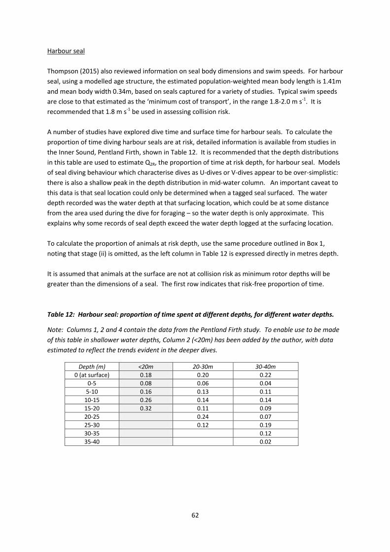
62

Harbour seal

Thompson (2015) also reviewed information on seal body dimensions and swim speeds. For harbour

seal, using a modelled age structure, the estimated population-weighted mean body length is 1.41m

and mean body width 0.34m, based on seals captured for a variety of studies. Typical swim speeds

are close to that estimated as the ‘minimum cost of transport’, in the range 1.8-2.0 m s-1. It is

recommended that 1.8 m s-1 be used in assessing collision risk.

A number of studies have explored dive time and surface time for harbour seals. To calculate the

proportion of time diving harbour seals are at risk, detailed information is available from studies in

the Inner Sound, Pentland Firth, shown in Table 12. It is recommended that the depth distributions

in this table are used to estimate Q2R, the proportion of time at risk depth, for harbour seal. Models

of seal diving behaviour which characterise dives as U-dives or V-dives appear to be over-simplistic:

there is also a shallow peak in the depth distribution in mid-water column. An important caveat to

this data is that seal location could only be determined when a tagged seal surfaced. The water

depth recorded was the water depth at that surfacing location, which could be at some distance

from the area used during the dive for foraging – so the water depth is only approximate. This

explains why some records of seal depth exceed the water depth logged at the surfacing location.

To calculate the proportion of animals at risk depth, use the same procedure outlined in Box 1,

noting that stage (ii) is omitted, as the left column in Table 12 is expressed directly in metres depth.

It is assumed that animals at the surface are not at collision risk as minimum rotor depths will be

greater than the dimensions of a seal. The first row indicates that risk-free proportion of time.

Table 12: Harbour seal: proportion of time spent at different depths, for different water depths.

Note: Columns 1, 2 and 4 contain the data from the Pentland Firth study. To enable use to be made

of this table in shallower water depths, Column 2 (<20m) has been added by the author, with data

estimated to reflect the trends evident in the deeper dives.

Depth (m) <20m 20-30m 30-40m

0 (at surface) 0.18 0.20 0.22

0-5 0.08 0.06 0.04

5-10 0.16 0.13 0.11

10-15 0.26 0.14 0.14

15-20 0.32 0.11 0.09

20-25 0.24 0.07

25-30 0.12 0.19

30-35 0.12

35-40 0.02

63

Grey seal

For grey seal, there are minor differences between the populations in the North Sea, Orkney and the

Hebrides, reflecting differences in sex and age structure. Population-weighted mean values have

been used as standard, with a 50:50 sex ratio, giving a mean body length of 1.86m, body width

0.42m.

As for harbour seal, research on swim speeds for grey seal indicate that foraging swim speeds are

close to the estimated minimum cost of transport speed, in the range 1.8-2.0 m s-1. It is

recommended that a swim speed of 1.8 m s-1 be used for collision risk assessment.

Studies by Beck et al. (2000) have illustrated the dive cycle parameters for grey seal, indicating a

mean dive cycle of 462 secs, including a mean of 165 secs surface time. The studies did not

discriminate between U-dives and V-dives, but they did note differences between pre-moult seals

and post-breeding seals.

Dive depth data from a study in the Pentland Firth has provided detailed data on the proportion of

time spent at various depths (Table 13). It is recommended that the depth distributions in this table

are used to estimate Q2R, the proportion of time at risk depth, for grey seal. Use the same procedure

as for harbour porpoise, except that stage (ii) should be omitted, as the depth ranges are expressed

directly in metres depth. The data are subject to the same caveat as for harbour seals, as to the

uncertainty associated with water depth. The first row indicates the proportion of time at the

surface, assumed to be free of collision risk.

Table 13: Grey seal: proportion of time spent at different depths, for different water depths

Dive depth bin (m)

Proportion of time in each depth bin for dives in different water depths

<20m 20-30m 30-40m 40-50m 50-60m >60m

0 (at surface) 0.18 0.18 0.18 0.18 0.18 0.18

0-5 0.02 0.02 0.02 0.02 0.02 0.02

5-10 0.12 0.05 0.04 0.10 0.09 0.09

10-15 0.14 0.10 0.05 0.10 0.16 0.11

15-20 0.19 0.12 0.08 0.10 0.12 0.10

20-25 0.34 0.27 0.09 0.07 0.11 0.11

25-30 0.22 0.10 0.07 0.05 0.08

30-35 0.05 0.19 0.07 0.05 0.06

35-40 0.19 0.07 0.03 0.04

40-45 0.06 0.07 0.03 0.04

45-50 0.07 0.03 0.02

50-55 0.06 0.03 0.02

55-60 0.04 0.02

60-65 0.05 0.03

65-70 0.03

70-75 0.03

75+ 0.01

64

Minke whale

Body length and swim speed for minke whale are taken from Batty et al. (2012), quoting Horwood

(1990) for body length and Williams (2009) for swim speed. Body width (used in the CRM) is taken

as one quarter of the animal’s length. Mean dive time is calculated by averaging over a typical cycle

of five dives (four short, one long) as described by Stern (1992). Surfacing time is described by

Heide-Jørgenson & Simon.

Basking shark

Adult basking shark body length ranges from 4-10m, with 7m being the average body length of

basking sharks observed in Scottish waters (Speedie et al. 2009). Swim speed is drawn from Sims

(2000).

Figure 11: Basking shark depth behaviour from Witt et al. 2014.

In a basking shark tagging project (Witt et al. 2014), a number of basking shark were tagged for

periods of over 200 days, and the use of different depths recorded. Figure 11 shows the mean

frequency of use of different depths for the six tagged shark reported in Figure 23 of that report.

The shark were free to roam in waters of a wide range of depths, and the deepest dive recorded was

to over 1000m depth. No information is available in this report about the use of different depths in

waters of restricted depth, such as occurs in the tidal channels best suited to tidal energy. The

reported data supports the view that basking shark frequent all depths from surface to seabed. Sims

(2000) observes that basking shark dive behaviour is variable, being highly dependent on where the

food source is in the water column. In the absence of more detailed information, for use in the

collision model it is recommended that a uniform depth distribution is assumed.

65

Atlantic salmon

Data has recently become available on the swim depths of homing Atlantic salmon in Scottish waters

(Godfrey et al. 2015). This data has been used as the basis for an empirical curve fitted to the

cumulative frequency f(h) as a function of depth h (the proportion of salmon swimming above each

depth), valid for depths up to 100m (see Figure 12):

f(h) = -7.5e-07 h4 + 2.4 e-04 h3 -2.71 e-02 h2 +1.274 h + 77.091 (45)

It is recommended that the depth distribution in equation (45) is used to estimate Q2R for adult

salmon. This formula is embedded in the Q2R function used in the spreadsheets. It should be noted

that the proportions of salmon swimming below about 35m are so small that the distribution may be

considered independent of seabed depth for water depths in the range 35-100m.

8.2 Diving birds

Robbins et al. (2014) have reviewed data on diving bird dimensions and dive behaviour from a

number of studies, and for one species (European shag) have been able to present mean values

across these studies which can be used with a fair degree of confidence. For two other species (red-

throated diver and black guillemot) the authors attribute moderate confidence to the mean data.

Such data are coloured deep orange (high confidence) or pale orange (moderate confidence)

respectively. For other species (uncoloured) their confidence is described as low or poor. For the

remaining species, the figures in the tables (uncoloured) are based on single studies, and are offered

here only as a starting point; they are not based on a comprehensive search of the literature.

At the time of this being written (April 2016), it is expected that the data in this diving birds section

will be updated later in 2016. Users should check that the most recent versions of these tables are

used.

Figure 12: Depth of homing Atlantic salmon from Godfrey et al. showing fit of equation (45)

66

Table 14: Diving birds - data on dimensions and swim style

Common name Scientific name

length (m)

wingspan (m) swim style

common eider Somateria mollissima

0.60 0.94 foot-propelled

red-throated diver Gavia stellata 0.61 1.11 foot-propelled

northern gannet Morus bassanus

0.94 1.72 wing-propelled

cormorant Phalacrocorax carbo

0.90 1.45 foot-propelled

European shag Phalacrocorax aristotelis

0.72 0.98 foot-propelled

black guillemot Cepphus grylle

0.31 0.55 wing-propelled

common guillemot Uria aalge 0.40 0.67 wing-propelled

razorbill Alca torda 0.38 0.66 wing-propelled

Atlantic puffin Fratercula arctica

0.28 0.55 wing-propelled

from BTO Bird Facts

Table 15: Diving birds - data on dive patterns

dive depth (m)

ascent speed (m s

-1)

descent swim speed (m s

-1)

dive underwater duration tu (s)

pause duration (s)

dives/ bout

dive frequency during diving bouts F2 (s

-1)

source of dive info

common eider

25.9 0.0191 Guillemette (2004)

red-throated diver

5.3 26.1 12.2 Robbins et al. (2014)

northern gannet

cormorant 40 0.00685 Snow & Perrins (2008)

European shag

23.2 1.5 1.8 41.7 33.8 20.9 0.0132 Robbins et al. (2014)

black guillemot

26.5 77.1 31.2 8.75 0.0092 Robbins et al. (2014)

common guillemot

77.6 0.0087 Evans et al. (2013)

Atlantic puffin

48.7 Spencer (2012)

Table 16: Diving birds - data on foraging trips

forage trip frequency G (trips/day)

forage trip duration U (s)

dives/trip dive frequency while foraging (s

-1)

67

red-throated diver

10 2388 Robbins et al. (2014)

European shag 2.8 5472 26.6 0.00486 Robbins et al. (2014)

8.3 Avoidance rates

There has as yet been insufficient monitoring of wildlife responses at operational tidal arrays to

enable avoidance rates to be assessed.

The avoidance factors which have been applied to date in various environmental assessments are

the result of professional judgement by ecologists involved in each project on what they considered

was the likely potential for successful avoidance (both active and passive) by the different life stages

of the different species. Given the present lack of knowledge of avoidance behaviour, SNH

recommends that all collision risk assessments using an avoidance factor should set out results using

six avoidance rates: 0% (i.e. no avoidance), 50%, 90%, 95%, 98% and 99%. The Avoidance sheet of

the attached spreadsheet applies these rates automatically to the results of both the ERM and CRM

models.

As our knowledge of animal behaviour in proximity to tidal turbines improves, species-specific

avoidance rates may be refined. Therefore it is advised that avoidance rates should be agreed with

the Regulators at an early stage in the assessment.

68

SECTION 9: REFERENCES

Bailey, K.M. & Batty, R.S. 1983. A laboratory study of predation by Aurelia aurita on larval herring: experimental observations compared with model predictions. Marine Biology 72, 295-301.

Band, W. 2000. Windfarms and Birds: calculating a theoretical collision risk assuming no avoiding

action. Scottish Natural Heritage Guidance Note. www.snh.gov.uk/planning-and-

development/renewable-energy/onshore-wind/assessing-bird-collision-risks/

Band, W., Madders, M. & Whitfield, D.P. 2007. Developing field and analytical methods to assess

avian collision risk at windfarms. In: De Lucas, M., Janss, G. and Ferrer, M. (eds) Birds and Wind

Power. www.quercus.pt

Band, W. 2012a. Using a collision risk model to assess bird collision risks for offshore windfarms. The Crown Estate Strategic Ornithological Support Services (SOSS) report SOSS-02. SOSS Website. Original published Sept 2011, extended to deal with flight height distribution data March 2012. www.bto.org/science/wetland-and-marine/soss/projects

Band, W. 2012b. MeyGen tidal stream array: comments on marine mammal collision risk assessment. Report for Scottish Natural Heritage, unpublished.

Band, W. 2014. Detailed Collision Risk Assessment: Marine mammals, Basking shark, and Diving Birds. In Fall of Warness test site Environmental Appraisal: Annex 7. EMEC.

Batty, R.S., Benjamins, S. & Wilson, B. 2012. MeyGen tidal-stream turbine array environmental impact assessment: modelling encounter rate between turbines and animals. SRSL. Commercial in confidence.

Beck, C., Don Bowen, W., Iverson, S.J . (2000). Seasonal changes in buoyancy and diving behaviour of adult grey seals. Journal of Experimental Biology 203, 2323-2330.

Birdlife International. www.birdlife.org/datazone/speciesfactsheet.php?id=3679 accessed Dec 2014.

BTO Bird Facts: www.bto.org/about-birds/birdfacts British Trust for Ornithology, website

Buckland, S.T., Anderson, D.R., Burnham, K.P., Laake, J.L., Borchers, D.L. & Thomas, L. 2001. Introduction to distance sampling. Oxford University Press.

Cairns, D.K. Diving behaviour of Black guillemots in north-eastern Hudson Bay. 1992. Colonial waterbirds 15, 245-248.

Camphuysen, C.J., Fox, A.D., Leopold, M.F. & Petersen, I.K. 2004. Towards standardised seabirds at

sea census techniques in connection with environmental impact assessments for offshore wind farms

in the UK. Cowrie.

Chudzinska, M. 2009. Diving behaviour of harbour seals (Phoca vitulina) from the Kattegat. Masters Thesis, University of Aarhus and Danish National Environmental Research Institute.

69

Evans, T.J., Kadin, M.,Olsson, O. & Akesson, S. 2013. Foraging behaviour of common murres in the Baltic Sea, recorded by simultaneous attachment of GPS and time-depth recorder devices. Marine Ecology Progress Series 475, 277-289.

Evans, P.G.H., Baines, M.E. & Coppock, J. 2011. Abundance and behaviour of cetaceans and basking sharks in the Pentland Firth and Orkney Waters. Report by Hebog Environmental Ltd & Sea Watch Foundation. Scottish Natural Heritage Commissioned Report 419. www.snh.org.uk/pdfs/publications/commissioned_reports/419.pdf Forsythe, W.C., Rykiel, E.J., Jr, Stahl, R.S., Wu, H., & Schoolfield, R.M. (1995). A model comparison

for daylength as a function of latitude and day of year. Ecological Modelling 80, 87-95.

Garthe, S., Benvenuti, S. & Montevecchi, W.A. 2000. Pursuit plunging by northern gannets feeding on capelin. Proceedings of the Royal Society of London B 267, 1717-1722

Garthe, S., Benvenuti, S., Montevecchi, W.A. 2003. Temporal patterns of foraging activities of northern gannets in the north-west Atlantic Ocean. Canadian Journal of Zoology 81, 453-461.

Gerritsen, J. & Strickler, R. 1976. Encounter probabilities and community structure in zooplankton: a mathematical model. Journal of the Fisheries Research Board of Canada 34, 73-82

Godfrey, J.D., Stewart, D.C., Middlemas, S.J. & Armstrong, J.D. 2015. Depth use and migratory behaviour of homing Atlantic salmon (Salmo salar) in Scottish coastal waters. ICES Journal of Marine Science, Early View July 2014. doi.10.1093/icesjms/fsu118

Grant, M.C., Trinder, M., & Harding, N.J. 2014. A diving bird collision risk assessment framework for tidal turbines. Scottish Natural Heritage Commissioned Report No 773. www.snh.org.uk/pdfs/publications/commissioned_reports/773.pdf

Guillemette, M., Woakes, A. J., Henaux, V., Grandbois, J.M. & Butler, P. J. 2004. The effect of depth on the diving behaviour of Common Eiders. Canadian. Journal of Zoology 82, 1818-1826.

Heide-Jørgenson, P. & Simon, M. Cue rates for common minke, fin and humpback whales in West Greenland. Greenland Institute of Natural Resources, Nuuk.

Horwood, J. 1990. Biology and exploitation of the minke whale. CRC Press, Florida 1990.

Joint Nature Conservation Committee, European Seabirds at Sea database. www.jncc.defra.gov.uk/page-1547. Web page last updated 2009.

Jones, E.L., McConnell, B.J., Smout, S., Hammond, P.S., Duck, C.D., Morris, C.D., Thompson, D., Russell, D.J.F., Vincent, C., Cronin, M., Sharples, R.J. & Matthiopoulos, J. 2015. Patterns of space use in sympatric marine colonial predators reveal scales of spatial partitioning. Marine Ecology Progress Series, 534, 235–249.

Jones, E.L., Smout, S., Blight, C., Sparling, C.E. & McConnell, B.J. 2016. Fine-scale harbour seal usage around Orkney. Report commissioned by Marine Scotland MSQ074 under contract CR/2014/11.

Marine Scotland, 2011. Topic sheet 18 v2: Scottish Salmon Sea-Ages from Length or Weight and Return-Date.

ORJIP Ocean Energy, 2015. The Forward Look: an ocean energy environmental research strategy for the UK. Report to The Crown Estate, Marine Scotland and Welsh Government. Aquatera Ltd and MarineSpace.

70

Otani, S., Naito, Y., Kato, A. & Kawamura, A. 2000. Diving behaviour and swimming speed of a free-ranging harbour porpoise Phocoena phocoena. Marine Mammal Science 16, 811-814.

Polak, M. & Ciach, M. 2007. Behaviour of black-throated diver and Red-throated diver during autumn migration stopover. Ornis Svecica 17, 90-94

Robbins, A.M.C, Furness, R.W., Thaxter, C.B., Daunt, F.H., Cook, A.S.C.P. & Masden, E.A. 2014. A review of marine diving bird behaviour: assessing underwater collision risk with tidal turbines. Proceedings of the 2nd International Conference on environmental interactions of marine renewable energy technologies. EIMR 2014, 573. www.eimr.org

Scott-Hayward, L., Oedekoven,C., Mackenzie, M. & Rexstad, E. (2013). Statistical Modelling of

Seabird and Cetacean data Users Guide: Using the MRSea Package. Centre for Research into

Ecological and Environmental modelling. On Marine Scotland website:

http://www.gov.scot/Topics/marine/marineenergy/Research/SB9/UsingMRSea

Scottish Natural Heritage / Royal Haskoning (2011). Guidance on Survey and Monitoring in relation to Marine Renewables Deployments in Scotland. Prepared for Scottish Natural Heritage and Marine Scotland by Royal Haskoning, with input from the Sea Mammal Research Institute, Natural Research and Graham Saunders Marine Ecology. In draft. http://www.snh.gov.uk/docs/B925810.pdf

Sea Mammal Research Unit, University of St Andrews (2006). Small Cetaceans in the European Atlantic and North Sea (SCANS-II). European LIFE project led by SMRU. http://biology.st-andrews.ac.uk/scans2/inner-finalReport.html Sea Mammal Research Unit, University of St Andrews (2014). Grey and harbour seal usage maps. Published on Scottish Government’s Marine Scotland Website: www.scotland.gov.uk/Topics/marine/science/MSInteractive/Themes

Sims, D.W. 2000. Filter feeding and cruising swimming speeds of basking sharks compared with optimal models. Journal of Experimental Marine Biology and Ecology 249, 65-76.

Sims, D.W., Southall, E.J., Tarling, G.A. & Metcalfe, J.D. 2005. Habitat-specific normal and reverse diel vertical migration in the plankton-feeding basking shark. Journal of Animal Ecology 74, 755-756.

Sims, D.W. 2008. Sieving a living: a review of the biology, ecology and conservation status of the plankton-feeding basking shark Cetorhinus maximus. Advances in Marine Biology 54, 171-219.

Snow, D.W., & Perrins, C.M. 1998. The Birds of the Western Palaearctic. Concise edition (Vol 2). Oxford University Press.

Speedie, C.D., Johnson, L.A. & Witt, M.J. 2009. Basking shark hotspots on the West Coast of Scotland: key sites, threats and implications for conservation of the species. Scottish Natural Heritage Commissioned Report No 339.

Spencer, S.M. 2012. Diving behaviour and identification of sex of breeding Atlantic puffins, and nest-site characteristics of alcids on Petit Manan Island, Maine. Masters Thesis, University of Massachusetts.

Stern, S.J. 1992. Surfacing rates and surfacing patterns of minke whales (Balaenoptera acutorostrata) off Central California, and the probability of a whale surfacing within visual range. Report of the International Whaling Commission 42, 379-385.

71

Stone, C.J., Webb, A., Barton, C., Ratcliffe, N., Reed,T.C., Tasker,M.L., Camphuysen, C.J. & Pienkowski, M.W. 1995. An Atlas of seabird distribution in north-west European waters. Joint Nature Conservation Committee 1995.

Teilmann, J., Larsen, F., & Desportes, G. 2007. Time allocation and diving behaviour of harbour porpoises (Phocoena phocoena) in Danish and adjacent waters. Journal of Cetacean Research and Management 9, 201-210.

Thaxter, C.B., Wanless, S., Daunt, F., Harris, M.P., Benvenuti, S., Watanuki, Y., Grémillet, D. & Hamer, K.C. 2010. Influence of wing loading on the trade-off between pursuit-diving and flight in common guillemots and razorbills. Journal of Experimental Biology 213, 1018-1025.

Thompson, D., Onoufriou, J., Brownlow, A. & Morris, C. 2014a. Data based estimates of collision risk: an example based on harbour seal tracking data around a proposed tidal turbine array in the Pentland Firth. Report by the Sea Mammal Research Unit, University of St Andrews, for Scottish Natural Heritage and Marine Scotland.

Thompson, D., Brownlow, A., Onoufriou, J. & Moss, S. 2014b. Collision risk and impact study: field tests of turbine blade-seal carcass collisions. Report by the Sea Mammal Research Unit, University of St Andrews, for Scottish Natural Heritage and Marine Scotland.

Thompson, D. 2015. Parameters for collision risk models. Report by Sea Mammal Research Unit, University of St Andrews, for Scottish Natural Heritage.

Wanless, S., Corfield T., Harris M.P., Buckland S.T. & Morris J.A. 1993. Diving behaviour of the shag Phalacrocorax aristotelis in relation to water depth and prey size. Journal of Zoology 231, 11-25.

Westgate, A.J., Head, A.J., Berggren, P., Koopman, H.N. & Gaskin, D.E. 1995. Diving behaviour of harbour porpoises Phocoena phocoena. Canadian Journal of Fisheries and Aquatic Sciences 52, 1064-73.

Williams, T.M. (2009). Encyclopedia of Marine Mammals 1140-47. ed Perrin, W.F., Würsig, B. and Thewissen, J.G.M. Academic Press (2009).

Wilson, B., Batty, R.S., Daunt, F. & Carter, C. 2007. Collision risks between marine renewable energy devices and mammals, fish and diving birds. Report to the Scottish Executive by the Scottish Association for Marine Science.

Witt, M.J., Doherty, P.D., Godley, B.J., Graham, R.T., Hawkes, L.A. & Henderson, S.M. 2014. Basking shark satellite tagging project: Insights into basking shark (Cetorhinus maximus) movement, distribution and behaviour using satellite telemetry (Phase 1, July 2014). Scottish Natural Heritage Commissioned Report 752. http://www.snh.org.uk/pdfs/publications/commissioned_reports/752.pdf

Xodus Environment. 2012. Estimating encounter rate for Atlantic salmon for the MeyGen Tidal

Energy Project, Phase 1 and potential population effects. Technical note for Meygen Environmental

Statement.

72

SECTION 10: WORKED EXAMPLES

In this section, four worked examples are described, to illustrate application of the three models and

use of the spreadsheet in different circumstances. The first two worked examples are based on an

assessment of potential collision risk with marine animals and diving birds at the EMEC tidal test site

on Orkney (Band 2014). EMEC provided survey data, derived from a regular wildlife survey of the

site, counting sightings of both diving birds and marine animals, from July 2005 – March 2014. The

third is based on one of the worked examples outlined by Grant et al. (2014), considering the

collision risk of a hypothetical tidal array in the Pentland Firth with European shags. The final

worked example is based on an assessment of collision risk with Atlantic salmon, undertaken for the

Meygen development in the Pentland Firth (Xodus Environment 2012). Please note, however, that

the results presented in this worked example may differ from the original assessment due to the use

the standard parameters recommended in Section 8.

The calculations are shown in the Tables WE1 – WE4 below. These calculations may be reproduced

using the spreadsheet accompanying this guidance, and this is recommended for anyone

familiarising themselves with the calculations.

WE1: Fall of Warness, Orkney – marine animals

The calculations for this worked example are shown in Tables WE1 (i) – (iii). These three worksheets

calculate respectively (i) animal density at risk depth, (ii) the ERM encounter rate and (iii) the CRM

collision rate. Species assessed were harbour porpoise, harbour seal, grey seal, minke whale and

basking shark.

(i) Marine animals – density at risk depth

Observed density

The data input here DS is the density of animals at the sea surface, as derived from the EMEC survey

observations, after undertaking distance correction and allocation of unidentified species (i.e.

Stages 1 and 2 of the survey data processing as described in section 3). Stage 3 (adjusting for

nocturnal activity) was omitted for marine animals as, in the absence of contrary information, it was

assumed that nocturnal activity was at the same level as during daytime.

Proportion of animals visible at surface

Figures for mean underwater dive duration, and mean surface time, are drawn from Table 10 in

Section 8, and are used in these columns to calculate the overall dive frequency, and the proportion

visible at the surface. For basking shark, no correction for the proportion of time underwater is

made at this stage, and so the fields for ‘mean underwater duration of dive’ and ‘mean surface time’

are left blank.

Watch time had not been specified or controlled during the survey; however, knowing the time

allotted for a complete scan, and the field width of the binoculars used, an estimate was made that

the watch time for each area of sea viewed through the binoculars could only be around 10-15 secs.

10 seconds was used in the calculations, erring on the precautionary side (a shorter watch period

means a greater multiplying factor to allow for animals underwater).

73

The adjusted at sea density DA is then the observed density DS divided by the proportion visible at

the surface.

Risk depth

Collision risks were assessed for a reference 3-blade turbine of 25m diameter. It was assumed that

the rotors would be sited with rotor tips at a minimum depth of 2.5m, so that a rotor would not

breach the surface and encounter animals at the surface. For many species, risk decreases with

depth below the surface so 2.5m was selected as a ‘worst case’ in terms of possible rotor depths. An

average channel depth of 30m was assumed. Thus the 25m diameter rotors were assumed to

occupy most of the depth range, from 2.5 – 27.5m.

Proportion of animals at risk depth

To calculate the animal density at risk depth, depth distribution models were selected according to

species:

for harbour porpoise, the ‘harbour porpoise’ model was selected, based on a researched

species-specific depth distribution;

for harbour seal, the ‘harbour seal U-dive’ model was selected, based on the species-specific

depth distribution described in Section 8 Table 12;

for grey seal, it was not known whether U-dives or V-dives would be prevalent. The ‘deep-

diving’ generic model depth distribution was used – this calculates the time a seal takes to swim

across the diameter of a rotor during both descent and ascent. A vertical swim speed of

1.4 m s-1 was assumed.

for minke whale and basking shark, a ‘uniform’ depth distribution throughout the channel

depth was assumed.

Using the inbuilt function Q2R which does the calculation appropriate to the selected depth

distribution model, the spreadsheet then calculates the ‘proportion at risk depth’ and the ‘density at

risk depth’ D in animals m-3. This last is the key parameter which is fed in to the ERM and CRM

model worksheets.

It may be noted that for harbour and grey seal, the proportions at risk depth calculated using the

observed data in Tables 12 and 13 are much higher (by a factor of 2 or 3) than proportions calculated

using the deep-diving model. This may signal a more general warning that use of both the shallow

and deep-diving models to calculate the proportion of time at risk may significantly underestimate

time spent in mid-water column.

(ii) ERM worksheet

Period data

A period of one complete year was selected.

Rotor data

Turbine details assumed in this Worked Example are: 3-bladed turbines of diameter 25m, blade

width 0.75m from front to back, mean rotation speed of 6.95 rpm. Turbines non-operational for

12.4% of the time. Mean current speed during periods of operation 1.82 m s-1.

74

Animal data

For each species, the animal density at risk depth D is copied over from the previous worksheet.

All the species are classed as marine animals (this simply guides which parameters are used in the

ERM and CRM calculations). Mean animal length and bodywidth are input using the recommended

parameters in Table 10. The mean swim speed is a mean speed while foraging , relative to the

water, not taking into account any extra speed due to a tidal current. Cell E17 calculates a resultant

speed relative to the rotor, combining both current speed and animal swim speed.

Shape factor was taken to be 0.5, as for long thin objects (needle-shaped).

ERM encounter rate

The worksheet calculates the effective animal radius and the effective blade area, taking account of

the clearance required to miss a blade, and then calculates the number of encounters expected in

the selected period (1 year) for the given animal density D. The ERM results indicate encounter

rates from 0.74 per year (grey seal) to 2.47 per year (harbour seal).

(iii) CRM worksheet

Period data

A period of one complete year was selected.

Rotor data

Diameter, number of blades, rotation speed, non-operational time and mean current speed were as

used in the ERM worksheet. For the CRM model, the maximum blade chord width was taken as

1.5m, with a pitch at the tip of 5 degrees relative to the rotor plane. (Note that a chord width of

1.5m is consistent with the choice of 0.75m as front-to-back width in the ERM; a blade of chord

width 1.5m at a pitch of 30 degrees would have a front-to-back width of 0.75m – refer to Figure 5.)

The tapering blade profile is expressed in the table showing the blade chord width as a fraction of

the maximum chord width at intervals r/R from 0 to 1 in 0.05 steps. This is the default taper in the

spreadsheet. If desired the table could be replaced by a blade profile table for the actual turbines,

though most turbine blades are broadly similar in profile.

Animal data

As in the ERM worksheet, all the species are classed as marine animals, mean animal length and

bodywidth are taken from Table 10.

CRM encounter rate

The worksheet calculates the total frontal area of the rotors, and hence (using the animal density)

the number of rotor transits in the period. Using the animal dimensions, the worksheet also

calculates the mean encounter probability for a single transit. Multiplying these gives the number of

encounters expected in the period.

The CRM results are in general quite similar to those of the ERM. The CRM estimates transit rates

through rotors between 1.0 (basking shark) and 8.4 (harbour seals) per year (see WE1 (iii) CRM:

‘number of rotor transits in period’), while the collision risk for any transit varies with animal size

from 30.8% (harbour seal) to 100% (minke whale and basking shark) (see same sheet ‘collision

75

probability for single transit’). Estimated collision rates (before avoidance) range from 0.9 per year

(grey seal) to 2.59 per year (harbour seal) – very similar to the ERM results.

76

Table WE1(i): Fall of Warness – marine animals - Density

Marine animals - density at risk depth

Species nameharbour

porpoiseharbour seal grey seal minke whale

basking

shark

Observed density (per m2) DS animals m-23.39890E-09 3.572E-09 1.056E-08 2.158E-10 1.083E-09

correct for proportion underwater? yes yes yes yes no

Proportion of animals visible at surface

mean underwater duration of dive tu s 26.2 180 297 87

mean surface time ts s 3.9 39.5 165 3.5

overa l l dive frequency F dives s-1

1/(tu+ts) 3.32E-02 4.56E-03 2.16E-03 1.10E-02 0.00E+00

watch period tw s 10 10.0 10.0 10.0 10.0 10.0

proportion vis ible at surface 1-F*max(0,tu-tw) 0.462 0.2256 0.379 0.149 1.000

adjusted at sea dens i ty DA animals m-27.36E-09 1.58E-08 2.788E-08 1.45E-09 1.08E-09

Risk depth

rotor diameter 2R m 25.0

rotor minimum depth m 2.5

channel depth m 30

Proportion of animals at risk depth

depth dis tribution typeharbour

porpoiseharbour seal deep-diving uni form uniform

vertica l swim speed u m s -11.40

time per dive at ri sk depth H s 35.71

proportion at ri sk depth Q2R FH 71.70% 52.50% 7.73% 83.33% 83.33%

dens ity at ri sk depth (per m3) D animals m-3DA Q2R /2R 2.11E-10 3.33E-10 8.62E-11 4.82E-11 3.61E-11

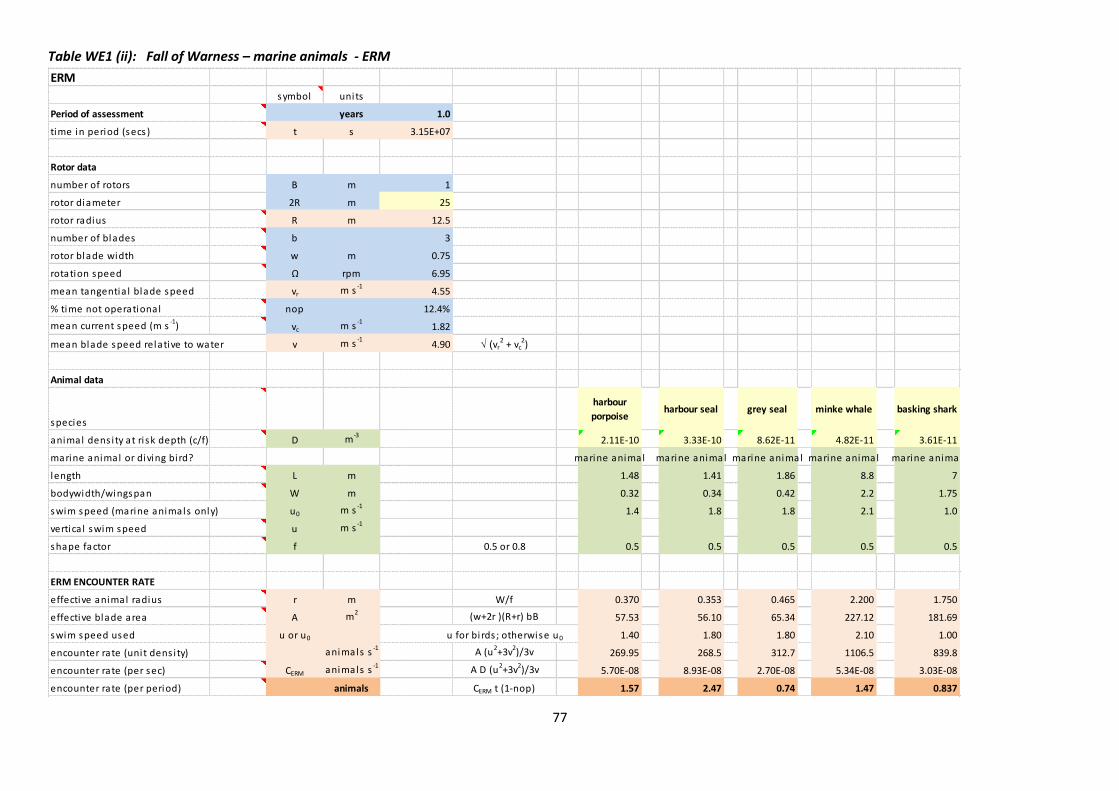
77

Table WE1 (ii): Fall of Warness – marine animals - ERM

ERM

symbol units

Period of assessment years 1.0

time in period (secs ) t s 3.15E+07

Rotor data

number of rotors B m 1

rotor diameter 2R m 25

rotor radius R m 12.5

number of blades b 3

rotor blade width w m 0.75

rotation speed Ω rpm 6.95

mean tangentia l blade speed vr m s -14.55

% time not operational nop 12.4%

mean current speed (m s-1

) vc m s-1

1.82

mean blade speed relative to water v m s -14.90 √ (vr

2 + vc2)

Animal data

species

harbour

porpoiseharbour seal grey seal minke whale basking shark

animal dens i ty at ri sk depth (c/f) D m-32.11E-10 3.33E-10 8.62E-11 4.82E-11 3.61E-11

marine animal or diving bird? marine animal marine animal marine animal marine animal marine animal

length L m 1.48 1.41 1.86 8.8 7

bodywidth/wingspan W m 0.32 0.34 0.42 2.2 1.75

swim speed (marine animals only) u0 m s -11.4 1.8 1.8 2.1 1.0

vertica l swim speed u m s -1

shape factor f 0.5 or 0.8 0.5 0.5 0.5 0.5 0.5

ERM ENCOUNTER RATE

effective animal radius r m W/f 0.370 0.353 0.465 2.200 1.750

effective blade area A m2

(w+2r )(R+r) bB 57.53 56.10 65.34 227.12 181.69

swim speed used u or u0 u for bi rds ; otherwise u0 1.40 1.80 1.80 2.10 1.00

encounter rate (unit dens i ty) animals s -1 A (u2+3v2)/3v 269.95 268.5 312.7 1106.5 839.8

encounter rate (per sec) CERM animals s -1 A D (u2+3v2)/3v 5.70E-08 8.93E-08 2.70E-08 5.34E-08 3.03E-08

encounter rate (per period) animals CERM t (1-nop) 1.57 2.47 0.74 1.47 0.837

78

Table WE1 (iii): Fall of Warness – marine animals - CRM

CRM blade profi le: r/R c/C

0 0.690

symbol units 0.050 0.730

Period of assessment years 1.0 0.100 0.790

time in period (secs ) t s 3.15E+07 0.150 0.880

0.200 0.960

Rotor data 0.250 1.000

number of rotors B m 1 0.300 0.980

rotor diameter (c/f) 2R m 25 0.350 0.920

rotor radius R m 12.5 0.400 0.850

number of blades b 3 0.450 0.800

maximum blade width C m 1.5 0.500 0.750

blade pi tch at blade tip γ degrees 5 0.550 0.700

blade profi le c/C <-- 0.600 0.640

rotation speed Ω rpm 6.95 0.650 0.580

% time not operational nop 12.4% 0.700 0.520

0.750 0.470

0.800 0.410

Current data 0.850 0.370

mean current speed (m s -1) vc m s -11.82 0.900 0.300

0.950 0.240

1.000 0.000

Animal data

Species (c/f)

harbour

porpoise

U-dives

harbour sealgrey seal minke whale

basking

shark

animal dens i ty ar ri sk depth (c/f) D animals m-3

2.11E-10 3.33E-10 8.62E-11 4.82E-11 3.61E-11

marine animal or diving bi rd? marine animal marine animal marine animal marine animal marine animal

length L m 1.48 1.41 1.86 8.80 7.00

wingspan / bodywidth W m 0.32 0.34 0.42 2.20 1.75

CRM ENCOUNTER RATE

body length used perp to rotor L' swap length & width for diving bi rds 1.48 1.41 1.86 8.80 7.00

body width used in rotor plane W' swap length & width for diving bi rds 0.32 0.34 0.42 2.20 1.75

speed of approach used vc m s -1vc 1.82 1.82 1.82 1.82 1.82

tota l fronta l area m2 Bπ(R+0.5W')2504 504 508 581 562

encounter probabi l i ty for s ingle trans i t pcol l pcol l 32.10% 30.77% 39.36% 100.00% 100.00%

no of rotor trans i ts per second s-1

D Bπ(R+0.5W')2 vc 1.93E-07 3.05E-07 7.96E-08 5.10E-08 3.69E-08

encounter rate (per sec) before avoidance CCRM D(Bπ(R+0.5W')2 vc pcol l 6.21E-08 9.39E-08 3.13E-08 5.10E-08 3.69E-08

no of rotor trans i ts in period D Bπ(R+0.5W')2 vc(1-nop)t 5.3 8.4 2.2 1.4 1.0

col l i s ions in period before avoidance animals CCRM (1-nop) t 1.72 2.59 0.9 1.4 1.0

ratio CRM/ERM 1.09 1.05 1.16 0.96 1.22

79

WE2: Fall of Warness, Orkney – diving birds

The calculations for this worked example are shown in Tables WE2 (i) –(iii). The three worksheets

calculate respectively (i) bird density at risk depth, (ii) the ERM encounter rate and (iii) the CRM

encounter rate. Species assessed were eider, red-throated diver, gannet, cormorant and black

guillemot.

(i) Diving birds – density at risk depth worksheet

Observed density

The data input here DS is the density of birds at the sea surface, as derived from the EMEC survey

observations, after undertaking distance correction and allocation of unidentified species (i.e.

Stages 1 and 2 of the survey data processing as described in section 3). Stage 3 (adjusting for

nocturnal activity) was only applied for cormorant and shag, as these species are known to be

relatively inactive at night: for these two species, nocturnal activity was set to zero.

Proportion of diving birds visible at surface

Method 1 was used to calculate the overall dive frequency, using values sourced from research

literature on dive frequency while foraging, and on the proportion of time foraging. Values for the

latter are scarce, and the values used for species other than shag are no more than informed

estimates.

Figures for mean underwater dive duration, were as quoted in Section 8 Table 15, with the

exception of gannet, for which the source was Garthe et al. (2000 and 2003). Mean dive duration

was then used to calculate the proportion visible at the surface and the adjusted at sea density DA.

Watch time had not been specified or controlled during the survey; however the observations were

described as snapshot counts, implying that watch time of any one area of sea surface was minimal.

Watch time was therefore taken as zero.

The adjusted at sea density DA is then the observed density DS divided by the proportion visible at

the surface.

Special treatment is required for gannet. Survey data for gannet were based, as for other species,

on the density of birds observed on the water. For gannets, a sizeable proportion of the population

on site are likely to be airborne at any time, and therefore not available to the water-surface based

survey count. In contrast, the time spent underwater during dives is relatively short and of minimal

significance when considering the overall number on site, and may be ignored. Thus for gannet,

when considering availability to be counted in a water-surface-based survey, the time spent airborne

takes the place of the time underwater. The ‘proportion visible at the surface’ is the proportion of

the population on site including those birds airborne, and the ‘adjusted at sea density’ is the density

including birds airborne.

For gannet, data on foraging was drawn from Garthe et al. (2000 and 2003). Cell K9 (Gannet:

proportion of time foraging) was used to refer to the proportion airborne. The formula in Cell K18

(Gannet: proportion visible at the surface) was overwritten so as to calculate as (1 - proportion

airborne), thus becoming the proportion of gannet visible at the sea surface. The ‘adjusted at sea

80

density’ figure DA then expresses the areal density of gannets, including those in the air as well as

those on the surface.

A value for overall dive frequency was also available and was entered directly in cell K15 (gannet:

overall dive frequency), overwriting the formula there. This value is then used in the normal way in

the calculation of the proportion of birds at risk depth.

Risk depth

As in the previous Worked Example, the 25m diameter rotors were assumed to occupy most of the

depth range, from 2.5 – 27.5m.

Proportion of diving birds at risk depth

Eider and red-throated diver were assumed to be shallow-diving, that is, their dives do not go

deeper than the deepest parts of the rotor. Cormorant and black guillemot were assumed to be

deep-diving. Gannet are assumed to plunge-dive, that is they descend rapidly in a dive from the air,

then ascend at a more measured speed to the surface.

Vertical swim speeds – while in descent and ascent – determine the proportion of time at risk. A

figure of 1.65 m s-1 was taken as the mean of ascent and descent speeds for European shag (see

Section 8 Table 15). In the absence of species-specific data this figure was also used for cormorant,

eider and red-throated diver. For black guillemot, the figure of 1.48 m s-1 found by Thaxter et al.

(2010) for common guillemot was used.

For gannet, the descent speed of 4.3 ms-1 is much greater than the ascent speed of 1.2 ms-1, both

quoted by Garthe et al. (2000). Depth distribution type ‘plunge-diving’ is used, which ensures that

the time to descend and to ascend are calculated separately and added to yield the time per dive at

risk depth.

(ii) ERM worksheet

Period data

A period of one complete year was selected.

Rotor data

Turbine details used in this Worked Example are the same as for WE1: 3-bladed turbines of

diameter 25m, blade width 0.75m from front to back, with a mean rotation speed of 6.95 rpm, non-

operational for 12.4% of time. Mean current speed during periods of operation 1.82 m s-1.

Animal data

For each species, the animal density at risk depth D is copied over from the previous worksheet.

All the species are classed as diving birds. This forces the calculation to use the vertical swim speed,

not the horizontal swim speed, as the approach speed; for diving birds the horizontal swim speed is

not required. Mean bird length and wingspan are input, drawing data from Table 14. Vertical swim

speed is as in the density (diving birds) worksheet, except for gannet where a simple mean of the

descent and ascent speeds is used. Shape factor is taken to be 0.5 (as for marine animals) for birds

whose swimming action is foot-propelled, and 0.8 for wing-propelled birds which use their wings to

scull underwater.

81

ERM encounter rate

The worksheet calculates the effective animal radius and the effective blade area, taking account of

the clearance required to miss a blade, and then calculates the number of encounters for the

selected period (1 year) for the given diving bird density D.

(iii) CRM worksheet

Period data

A period of one complete year was selected.

Rotor data

Rotor parameters were as for the ERM model, except for blade width. For the CRM model, the

blade chord width was taken as 1.5m, with a pitch at the tip of 5 degrees relative to the rotor plane.

The tapering blade profile was expressed in the table showing the blade chord width as a fraction of

the maximum chord width at intervals r/R from 0 to 1 in 0.05 steps. This is the default taper in the

spreadsheet – data are not yet available on the taper of an actual tidal turbine.

Animal data

For each species, the animal density at risk depth D is copied over from the previous worksheet.

All the species are classed as diving birds. Mean bird length and wingspan are input, based on

various sources. Because the birds are assumed to be diving downwards or surfacing upwards, the

role of length L and wingspan W are interchanged in the subsequent calculation. Data on bird swim

speeds are not required as the mean approach-to-rotor speed is taken as the current speed.

CRM collision rate

The worksheet calculates the total frontal area of the rotors, and hence (using the animal density)

the number of rotor transits per second. Using the diving bird dimensions, it also calculates the

mean probability of encounter for a single transit. Multiplying these gives the number of collisions

expected per year (before taking account of avoidance).

The CRM estimates transit rates through rotors (penultimate row ‘no of rotor transits in period’)

between 0.3 (gannet) and 119 (eider) per year, while the mean risk of a collision for any transit

(collision probability for single transit) varies with animal size from 22% (eider) to 37% (gannet).

82

Table WE2 (i): Fall of Warness – diving birds- Density

Diving birds - density at risk depth

Species nameeider

red-throated

divergannet cormorant black guillemot

Observed density (per m2) DS birds m-23.08E-07 1.08E-08 3.67E-08 6.62E-08 5.71E-07

correct for proportion underwater? yes yes yes yes yes

Proportion of diving birds visible at surface

choose method for calculating overall dive frequency: method 1 method 1 method 2 method 1 method 1

method 1 proportion of time foraging P2 60% 40% 0.558 100% 37.33%

dive frequency foraging F2 dives s-1

1.91E-02 3.09E-02 6.852E-03 9.200E-03

method 2 foraging trips per day G trips/day 3 3 3 3

dives per foraging trip U dives/trip 6 6 6 6

overa l l dive frequency F dives s -1P2F2 or GU/(24*3600) 1.15E-02 1.236E-02 3.75E-04 6.85E-03 3.43E-03

mean underwater duration of dive tu s 25.90 26.10 10.90 40.00 77.10

watch period tw s 0 0.0 0.0 0.0 0.0 0.0

proportion vis ible at surface 1-F*max(0,tu-tw) 0.703 0.677 0.442 0.726 0.735

adjusted at sea dens i ty DA birds m-24.38E-07 1.59E-08 8.30E-08 9.12E-08 7.77E-07

Risk depth

rotor diameter 2R m 25.0

rotor minimum depth m 2.5

Proportion of diving birds at risk deptheider

red-throated

divergannet cormorant

black

guillemot

vertica l swim speed u m s-1

1.65 1.65 1.20 1.65 1.48

plunge speed u' m s -14.30

depth dis tribution typedeep, shal low or

plunge-diving

shal low-

diving

shal low-

diving

plunge-

divingdeep-diving deep-diving

time per dive at ri sk depth H s depends on dive type 22.87 23.07 8.24 30.30 33.78

proportion at ri sk depth Q2R FH 26.2% 28.5% 0.3% 20.8% 11.6%

Density at risk depth D birds m-3DA Q2R /2R 4.592E-09 1.818E-10 1.025E-11 7.577E-10 3.605E-09

83

Table WE2 (ii): Fall of Warness – diving birds - ERM

ERM

symbol units

Period of assessment years 1.0

time in period (secs ) t s 3.15E+07

Rotor data

number of rotors B m 1

rotor diameter 2R m 25

rotor radius R m 12.5

number of blades b 3

rotor blade width w m 0.75

rotation speed Ω rpm 6.95

mean tangentia l blade speed vr m s -14.55

% time not operational nop 12.4%

mean current speed (m s-1

) vc m s-1

1.82

mean blade speed relative to water v m s -14.90 √ (vr

2 + vc2)

Animal data

specieseider

red-

throated

diver

gannet cormorantblack

guillemot

animal dens i ty at ri sk depth (c/f) D m-34.59E-09 1.82E-10 1.02E-11 7.58E-10 3.60E-09

marine animal or diving bird? diving bird diving bird diving bird diving bird diving bird

length L m 0.6 0.61 0.94 0.9 0.31

bodywidth/wingspan W m 0.94 1.11 1.72 1.45 0.55

swim speed (marine animals only) u0 m s -1

vertica l swim speed u m s -11.65 1.65 2.75 1.65 1.48

shape factor f 0.5 or 0.8 0.5 0.5 0.8 0.5 0.8

ERM ENCOUNTER RATE

effective animal radius r m W/f 0.235 0.28 0.69 0.36 0.22

effective blade area A m2

(w+2r )(R+r) bB 46.61 50.02 84.11 56.92 45.41

swim speed used u or u0 u for bi rds ; otherwise u0 1.65 1.65 2.75 1.65 1.48

encounter rate (unit dens i ty) animals s -1 A (u2+3v2)/3v 237.0 254.4 455.4 289.4 229.2

encounter rate (per sec) CERM animals s -1 A D (u2+3v2)/3v 1.09E-06 4.63E-08 4.67E-09 2.19E-07 8.26E-07

encounter rate (per period) animals CERM t (1-nop) 30.06 1.28 0.129 6.06 22.83

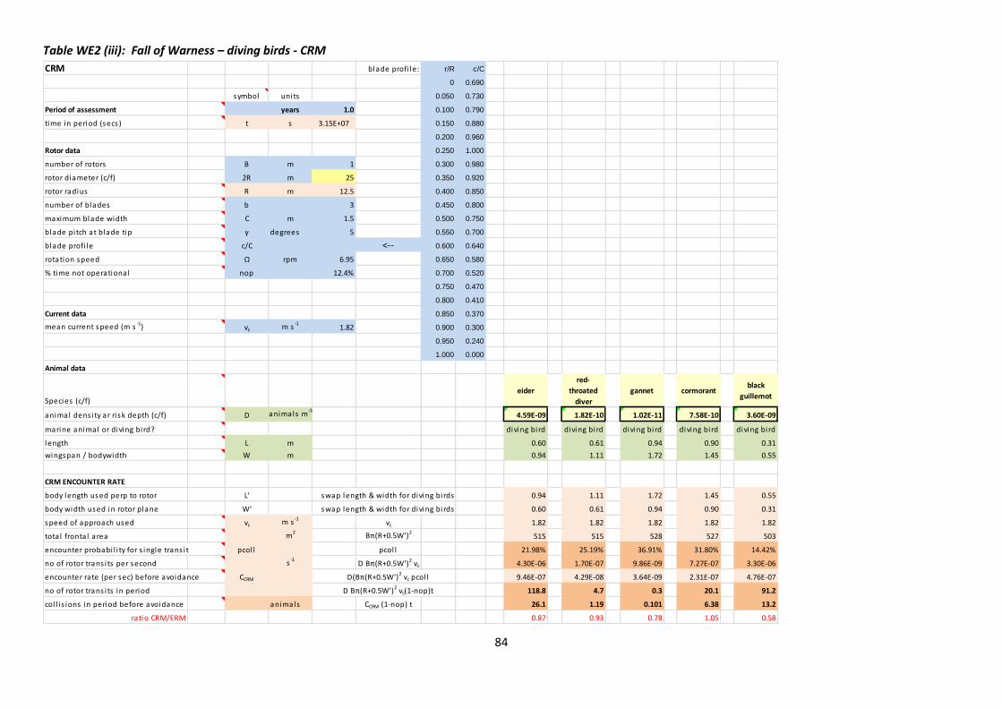
84

Table WE2 (iii): Fall of Warness – diving birds - CRM

CRM blade profi le: r/R c/C

0 0.690

symbol units 0.050 0.730

Period of assessment years 1.0 0.100 0.790

time in period (secs ) t s 3.15E+07 0.150 0.880

0.200 0.960

Rotor data 0.250 1.000

number of rotors B m 1 0.300 0.980

rotor diameter (c/f) 2R m 25 0.350 0.920

rotor radius R m 12.5 0.400 0.850

number of blades b 3 0.450 0.800

maximum blade width C m 1.5 0.500 0.750

blade pi tch at blade tip γ degrees 5 0.550 0.700

blade profi le c/C <-- 0.600 0.640

rotation speed Ω rpm 6.95 0.650 0.580

% time not operational nop 12.4% 0.700 0.520

0.750 0.470

0.800 0.410

Current data 0.850 0.370

mean current speed (m s -1) vc m s -11.82 0.900 0.300

0.950 0.240

1.000 0.000

Animal data

Species (c/f)eider

red-

throated

diver

gannet cormorantblack

guillemot

animal dens i ty ar ri sk depth (c/f) D animals m-34.59E-09 1.82E-10 1.02E-11 7.58E-10 3.60E-09

marine animal or diving bi rd? diving bi rd diving bi rd diving bi rd diving bi rd diving bi rd

length L m 0.60 0.61 0.94 0.90 0.31

wingspan / bodywidth W m 0.94 1.11 1.72 1.45 0.55

CRM ENCOUNTER RATE

body length used perp to rotor L' swap length & width for diving bi rds 0.94 1.11 1.72 1.45 0.55

body width used in rotor plane W' swap length & width for diving bi rds 0.60 0.61 0.94 0.90 0.31

speed of approach used vc m s -1vc 1.82 1.82 1.82 1.82 1.82

tota l fronta l area m2 Bπ(R+0.5W')2515 515 528 527 503

encounter probabi l i ty for s ingle trans i t pcol l pcol l 21.98% 25.19% 36.91% 31.80% 14.42%

no of rotor trans i ts per second s -1D Bπ(R+0.5W')

2 vc 4.30E-06 1.70E-07 9.86E-09 7.27E-07 3.30E-06

encounter rate (per sec) before avoidance CCRM D(Bπ(R+0.5W')2 vc pcol l 9.46E-07 4.29E-08 3.64E-09 2.31E-07 4.76E-07

no of rotor trans i ts in period D Bπ(R+0.5W')2 vc(1-nop)t 118.8 4.7 0.3 20.1 91.2

col l i s ions in period before avoidance animals CCRM (1-nop) t 26.1 1.19 0.101 6.38 13.2

ratio CRM/ERM 0.87 0.93 0.78 1.05 0.58

85

WE3: Pentland Firth – European shag

This worked example is drawn from Grant et al. (2014), section 3.5.2 of that paper. The calculations

are shown in Tables WE3 (i) and (ii) which calculate respectively the proportion of time spent at risk

depth by each bird on site, and the collision rate using the ETPM model which would cause a critical

adverse effect on the population. Only an outline is presented here – that paper should be

consulted for the population modelling aspects of the method, and for more detail on the choice of

input parameters.

A tidal array is envisaged comprising 100 turbines 20m diameter, sited within a seabed area of 1 km2

in the Pentland Firth. The blades are 0.5m deep back to front.

Exposure time is calculated, over a period of 12 months, for a population of European shag

potentially affected by the development.

The initial population size was set at 1181 individuals, based on an estimate of the adult breeding

population within a 20km radius of the site. January-April and August-December are treated as non-

breeding months, May as an incubation month, and June and July as chick-rearing months. Outwith

the breeding season, all 1181 were presumed to be foraging, while only 0.33 of the breeding adults,

plus all the immatures, totalling 775 birds, were presumed to be foraging at any one time during the

breeding season. Population modelling (not described in this guidance) led to an estimate that a

critical additional mortality of 60 birds per annum could lead to population decline.

Only a small proportion foraged at the development site, as there were other foraging areas within

range. The proportions were determined from boat survey counts of birds foraging within the site.

It is assumed that any necessary survey corrections – for distance/visibility, unidentified species,

nocturnal activity, watch time, or birds underwater – have already been made.

(i) Diving birds – density at risk depth

The diving birds density worksheet was used to establish the proportion of time spent at risk depth.

To get the overall dive frequency, method 2 was used, assuming 1 foraging trip per day during the

non-breeding and incubation months, and 3 foraging trips per day during the chick-rearing months.

Mean number of dives per foraging trip was taken as 26.6, drawn from Table 16, Section 8, with a

mean underwater dive duration of 41.7 seconds, drawn from Table 15. Using the ‘deep diving’

methodology of Section 4.4, and knowing the rotor diameter (20 m), and the vertical swim speed

(1.65 m s-1, the average of ascent and descent speeds in Table 15), the duration of dives at collision

risk depth was calculated at 24.2 seconds.

Multiplying by the overall dive frequency gives the proportion of time at risk depth as 0.75% in non-

breeding and incubation months, and 2.24% during the chick-rearing months. This data was then

transferred into the ETPM worksheet.

(Note that some rows are not used in deriving the proportion at risk depth: the observed density,

the watch period, the proportion visible at surface, the adjusted at-sea density, and the density at

risk depth. For this purpose, these rows can be ignored.)

86

(ii) ETPM worksheet

The ETPM worksheet is then used to calculate the exposure time within the rotor swept volume.

The analysis is subdivided into individual months as in Grant et al. (2014). No account was taken of

non-operational time, that is to say non-operational time was set to 0%. The effect of deeming a

proportion of time non-operational would be to reduce the time that each bird is exposed to the risk

of an operational turbine.

The site area is taken, as above at 1km2 or 106 m2. It is important that this is the same area within

which animal presence on site (‘number on site’) is counted.

The swept volume of each rotor is the volume of a cylinder of radius equal to the rotor radius R plus

half the animal length 0.5L as clearance (i.e. R+0.5L), and length equal to the depth of the rotor

blades from front to back w, plus half an animal length 0.5L clearance at both front and back, i.e.

(w+L)18. European shag were taken to be 0.72m long, from Table 14 in Section 8.

The ETPM worksheet then calculates, for each bird in the population, the total exposure time within

the rotor swept volume: 6.7 secs over a full year. Using the critical mortality of 60 birds leads to a

value for α of 0.00757: a collision rate, for each bird within the combined rotor swept volume of the

100 turbines, of 1 bird every 132 seconds. Using somewhat different input parameters Grant et al.

(2014) obtained a value of one collision every 452 secs for the required collision rate, and concluded

that the additional mortality resulting from collisions could well exceed that threshold and hence

could have a serious effect on the shag breeding population.

18

Note that Grant et al. (2014) allow for a full animal length L as clearance, both at the tip of the blades and at front and back when passing through the rotor, which leads them to slightly different results. Since the position of an animal is identified by some central point, 0.5L clearance is sufficient and is used here for consistency with the ERM and CRM approaches.

87

Table WE3 (i): Pentland Firth - European shag - Density

Diving birds - density at risk depth

other months Jun/July

Species name european shag european shag

Observed density (per m2) DS birds m-2

correct for proportion underwater? yes yes

Proportion of diving birds visible at surface

choose method for calculating overall dive frequency: method 2 method 2

method 1 proportion of time foraging P2 37.33% 37.33%

dive frequency foraging F2 dives s -19.950E-03 9.950E-03

method 2 foraging trips per day G trips/day 1 3

dives per foraging trip U dives/trip 26.6 26.6

overa l l dive frequency F dives s -1P2F2 or GU/(24*3600) 3.08E-04 9.24E-04

mean underwater duration of dive tu s 41.70 41.70

watch period tw s 0 0.0 0.0

proportion vis ible at surface 1-F*max(0,tu-tw) 0.987 0.961

adjusted at sea dens i ty DA birds m-2

0.00E+00 0.00E+00

Risk depth

rotor diameter 2R m 20.0

rotor minimum depth m 2.5

Proportion of diving birds at risk deptheuropean shag european shag

vertica l swim speed u m s-1

1.65 1.65

plunge speed u' m s -1

depth dis tribution typedeep, shal low or

plunge-divingdeep-diving deep-diving

time per dive at ri sk depth H s depends on dive type 24.24 24.24

proportion at ri sk depth Q2R FH 0.75% 2.24%

88

Table WE3 (ii): Pentland Firth – European shag - ETPM

ETPM

Period data Jan Feb Mar Apr May Jun Jul Aug Sep Oct Nov Dec all year

Period (days ) days 31 28 31 30 31 30 31 31 30 31 30 31 365

Period (seconds) t s days * 24*3600 2678400 2419200 2678400 2592000 2678400 2592000 2678400 2678400 2592000 2678400 2592000 2678400 31536000

Rotor data

area of s i te Asitem

21000000

number of rotors B m 100

rotor diameter 2R m 20 (c/f)

rotor radius R m 10

number of blades b 3

rotor width from front to back w m 0.5

% time not operational nop 0.0%

Animal data

species name European shag

target population N 1181 1181 1181 1181 1181 775 775 775 1181 1181 1181 1181 1181

number on s i te 14 9.9 18 7.5 10 6.4 14.1 12.3 13.9 3.6 12.4 2.2

proportion foraging on s i te P number on s i te/N 1.19E-02 8.38E-03 1.52E-02 6.35E-03 1.29E-02 8.26E-03 1.82E-02 1.04E-02 1.18E-02 3.05E-03 1.05E-02 1.86E-03

cri tica l added mortal i ty n 60

length L m 0.72

EXPOSURE TIME

prop of time at ri sk depth per bi rd on s i te Q2R FH 0.75% 0.75% 0.75% 0.75% 0.75% 2.24% 2.24% 0.75% 0.75% 0.75% 0.75% 0.75%

volume of sea at ri sk depth m320720000 (2R+L)*Asite

rotor swept volume Vrotor m3

41137 B π(R+0.5L)2 (w+L)

Vrotor as prop of volume at ri sk depth S 1.99E-03B π(R+0.5L) (w+L)/(2*Asite)

individual bi rd exposure time in Vrotor T s Q2R P S t (1-nop) 0.47 0.30 0.60 0.24 0.51 0.95 2.17 0.41 0.45 0.12 0.40 0.07 6.71

Collision rate

annual exposure time per bi rd T seconds 6.7

cri tica l col l i s ion rate per bi rd exposed αmax s-1

0.00757 n/NT

needs one col l i s ion every 1/αmax seconds 132

89

WE4: Pentland Firth - Atlantic salmon

This worked example is based on an assessment by Xodus Environment of the collision risk to

Atlantic salmon from a proposed array of 86 tidal turbines sited in the Pentland Firth (Xodus 2012),

but the method has been refined to make use of new depth distribution data. The calculations are

shown in Table WE4 (i) and (ii) which calculate respectively the proportion of salmon at risk depth

and, using the CRM model, the resulting collision rate before avoidance.

Estimates were compiled from a number of sources, including records from rivers throughout the

Scottish north and east coasts, of the total number of smolts and returning mature salmon migrating

through the Pentland Firth. Adult salmon were subdivided as grilse (one winter at sea) and MSW

(multiple sea winter) salmon. 88% were estimated to originate from east coast rivers, and 90%

were thought to migrate through more northerly channels.

It was assumed that each fish would make just one transit through the Firth per year, and that such

transits were uniformly distributed across the channel (eg they were not bunched close to shore).

This current example uses 6607314 smolts, 244969 grilse and 182672 MSW salmon as the estimated

number of salmon passages through the Pentland Firth in a year.

Such data lends itself to calculating the number of rotor transits per year directly, without

considering the areal density of fish. Additions have therefore been made to the CRM worksheet to

include these calculations.

(i) Density at risk depth

The proportion of salmon swimming at risk depth is calculated within the ‘Density – marine animals’

worksheet using the function within the spreadsheet for dive type ‘Atlantic salmon’; this is based on

data recently available on the swim depths of homing Atlantic salmon in Scottish waters (Godfrey et

al. 2014). Assuming that the 20m diameter turbines have a minimum depth of 8m yields a

proportion 10.6% of salmon within risk depth. This key figure is then copied forward into the CRM

worksheet. This figure has been used for all three age-classes of salmon though in reality smolts may

be much more concentrated within the surface 0-8m water layer.

(ii) CRM worksheet

This worksheet firstly calculates the mean collision probability for a single transit through a rotor,

using the CRM model. In this case the assumption in the CRM of perpendicular approach to the

rotor plane seems a reasonable model. Smolts will be swept by the tidal current, and the rotors

align themselves at right angles to the current. Migrating grilse and MSW salmon are thought likely

to be swimming with the current, using the current to aid their migration.

The proposed array consisted of 86 turbines, 20m diameter, 3 blades per rotor of maximum width

2.3m, pitch at blade tip 10 degrees and rotational speed 20rpm. It was assumed that installation

would have a minimum depth of 2.5m as a ‘worst case’. The proportion of non-operational time,

allowing for slack currents, was estimated at 17.3%. Fish dimensions are as estimated by Xodus

(2012): 15 cm x 2 cm (smolts), 67 cm x 12 cm (grilse), and 79 cm x 14 cm (MSW salmon). Swim

speed through the turbines was taken for all salmon types as the mean tidal speed (2.5 m s-1). For

grilse and MSW salmon, this may be an underestimate if the majority swim with the current. The

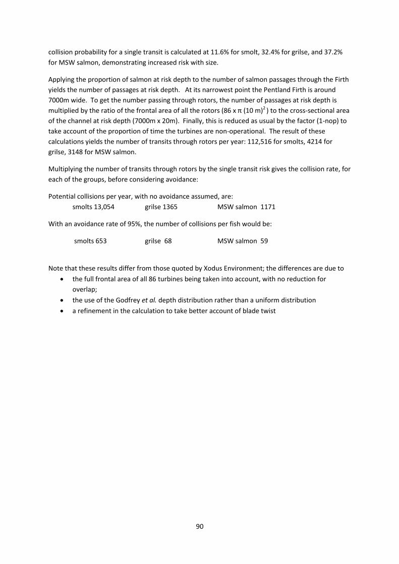
90

collision probability for a single transit is calculated at 11.6% for smolt, 32.4% for grilse, and 37.2%

for MSW salmon, demonstrating increased risk with size.

Applying the proportion of salmon at risk depth to the number of salmon passages through the Firth

yields the number of passages at risk depth. At its narrowest point the Pentland Firth is around

7000m wide. To get the number passing through rotors, the number of passages at risk depth is

multiplied by the ratio of the frontal area of all the rotors (86 x π (10 m)2 ) to the cross-sectional area

of the channel at risk depth (7000m x 20m). Finally, this is reduced as usual by the factor (1-nop) to

take account of the proportion of time the turbines are non-operational. The result of these

calculations yields the number of transits through rotors per year: 112,516 for smolts, 4214 for

grilse, 3148 for MSW salmon.

Multiplying the number of transits through rotors by the single transit risk gives the collision rate, for

each of the groups, before considering avoidance:

Potential collisions per year, with no avoidance assumed, are:

smolts 13,054 grilse 1365 MSW salmon 1171

With an avoidance rate of 95%, the number of collisions per fish would be:

smolts 653 grilse 68 MSW salmon 59

Note that these results differ from those quoted by Xodus Environment; the differences are due to

the full frontal area of all 86 turbines being taken into account, with no reduction for

overlap;

the use of the Godfrey et al. depth distribution rather than a uniform distribution

a refinement in the calculation to take better account of blade twist

91

Table WE4 (i): Pentland Firth – Atlantic salmon – Density

Marine animals - density at risk depth

Species name

Observed density (per m2) DS animals m-2

correct for proportion underwater?

Proportion of animals visible at surface

mean underwater duration of dive tu s

mean surface time ts s

overa l l dive frequency F dives s -11/(tu+ts)

watch period tw s 10

proportion vis ible at surface 1-F*max(0,tu-tw)

adjusted at sea dens i ty DA animals m-2

Risk depth

rotor diameter 2R m 20.0

rotor minimum depth m 8.0

channel depth m 35

Proportion of animals at risk depth

depth dis tribution typeatlantic

sa lmon

vertica l swim speed u m s -1

time per dive at ri sk depth H s

proportion at ri sk depth Q2R FH 10.65%

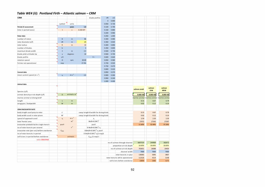
92

Table WE4 (ii): Pentland Firth – Atlantic salmon – CRM

CRM blade profi le: r/R c/C

0 0.690

symbol units 0.050 0.730

Period of assessment years 1.0 0.100 0.790

time in period (secs ) t s 3.15E+07 0.150 0.880

0.200 0.960

Rotor data 0.250 1.000

number of rotors B m 86 0.300 0.980

rotor diameter (c/f) 2R m 20 0.350 0.920

rotor radius R m 10 0.400 0.850

number of blades b 3 0.450 0.800

maximum blade width C m 2.3 0.500 0.750

blade pi tch at blade tip γ degrees 10 0.550 0.700

blade profi le c/C <-- 0.600 0.640

rotation speed Ω rpm 20.00 0.650 0.580

% time not operational nop 17.3% 0.700 0.520

0.750 0.470

0.800 0.410

Current data 0.850 0.370

mean current speed (m s-1

) vc m s-1

2.5 0.900 0.300

0.950 0.240

1.000 0.000

Animal data

Species (c/f)

salmon smoltsalmon

1SW

salmon

MSW

animal dens i ty ar ri sk depth (c/f) D animals m-30.00E+00 0.00E+00 0.00E+00

marine animal or diving bi rd? marine animal marine animal marine animal

length L m 0.15 0.67 0.79

wingspan / bodywidth W m 0.02 0.12 0.14

CRM ENCOUNTER RATE

body length used perp to rotor L' swap length & width for diving bi rds 0.15 0.67 0.79

body width used in rotor plane W' swap length & width for diving bi rds 0.02 0.12 0.14

speed of approach used vc m s-1

vc 2.50 2.50 2.50

tota l fronta l area m2 Bπ(R+0.5W')227072 27343 27397

encounter probabi l i ty for s ingle trans i t pcol l pcol l 11.60% 32.40% 37.20%

no of rotor trans i ts per second s -1D Bπ(R+0.5W')2 vc

encounter rate (per sec) before avoidance CCRM D(Bπ(R+0.5W')2 vc pcol l

no of rotor trans i ts in period D Bπ(R+0.5W')2 vc(1-nop)t

col l i s ions in period before avoidance animals CCRM (1-nop) t

ratio CRM/ERM

no of sa lmon through channel 6607314 244969 182672

proportion at ri sk depth 10.65% 10.65% 10.65%

no of sa lmon at ri sk depth 703651 26088 19454

channel width 7000 7000 7000

rotor trans i ts in year 136065 5095 3807

rotor trans i ts whi le operational 112526 4214 3148

col l i s ions before avoidance 13054 1365 1171

1

Cover image: Gulf of Corryvreckan, Patricia & Angus Macdonald / Aerographica.

Published: May 2016 (version 1)

Scottish Natural Heritage

Great Glen House

Leachkin Road

Inverness IV3 8NW

www.snh.gov.uk