guidance of an autonomous agent for coverage applications

Guidance of an Autonomous Agent for Coverage

Applications using Range Only Measurement

Twinkle Tripathy∗ and Arpita Sinha†

Systems & Control Engineering, IIT Bombay, Mumbai, Maharashtra, 400076, India

This paper addresses the problem of guiding an autonomous agent to cover a regionsurrounding a target. It is assumed that only range information is available to the agent.The target point is considered to be stationary. The region of interest can be changedby changing the initial conditions or the system parameters. In this work, we analyse theeffect of the initial conditions only. We propose a simple control law which can be easilyimplemented. The analytical results obtained here are validated through simulation. Theautonomous agent could be a ground or an aerial vehicle depending on the application. Forsurveillance applications, the target can be a landmark, where the agent can monitor theregion surrounding the landmark. Other applications can be sprinkling fertilizers, wateringa farm, etc. where a pre-defined area needs to be covered.

I. Introduction

The coverage problem refers to the problem of guiding an autonomous agent to cover an unknown orpredefined area. Several techniques have been proposed to achieve coverage, which vary depending on

the application.There are several algorithms which are used to cover unknown areas. For example, a lot ofwork has been done on map based coverage techniques (see [1], [2], [3], [4] and references therein) which workby dividing the area into cells and then assigning values to the cells based on the presence of obstacles orfree space. Wong et al.1 used topological maps to solve the coverage problem and their results are verifiedby simulation tests which show that over 99% of the surface is covered. The topological maps, representthe environment as graphs where landmarks are nodes, and edges represent the connectivity between thelandmarks. The algorithm achieves coverage with single mobile agent. Zelinsky et al.2 also use maps forcoverage but with a different approach. The solution ensures complete coverage by the use of a distancetransform path planning methodology. The solution was simulated and implemented on an autonomousrobot called Yamabico to give satisfactory performance. Stachniss et al.3 introduced the concept of coveragemaps where each cell of a given grid corresponds to the amount of a cell which is covered by an obstacle;the coverage maps are improvement of occupancy grids which are based on the assumption that each cellis either occupied or free. The model presented in the paper allows updation of the coverage maps uponinput obtained from sensors. Rutishauser et al.4 solve the problem of collaborative coverage using a swarmof networked miniature robots again by the use of grid based methods. For a multi-agent system, theproblem of coverage, addressed by Batavia et al.,5 has been solved with high accuracy for a semi- structuredenvironment. The approach has the advantage of an operator driving the outline of a desired coveragearea as input to a coverage generation algorithm. Acar et al.6 have solved the coverage problem by thedecomposition of the environment, by the use of voronoi diagrams.

Surveillance based systems, discussed in [7], [8] and [9], use wireless sensor networks to solve the coverageproblem. The sensor nodes are capable of behaving autonomously. In [7] and [9], the coverage achieved isaverage, but more emphasis is laid on the placement of sensors for effective coverage; Dhillon et al.7 havebased their work on fixed sensor nodes. Lai et al.8 discuss surveillance systems based on wireless sensornetworks. In [8], the deployed sensors are divided into disjoint subsets of sensors, or sensor covers, suchthat each sensor cover can cover all targets and work in turns. A surveillance system based on wireless

∗Research Scholar, Systems & Control Engineering, IIT Bombay and Student Member, AIAA.†Assistant Professor, Systems & Control Engineering, IIT Bombay

1 of 12

American Institute of Aeronautics and Astronautics

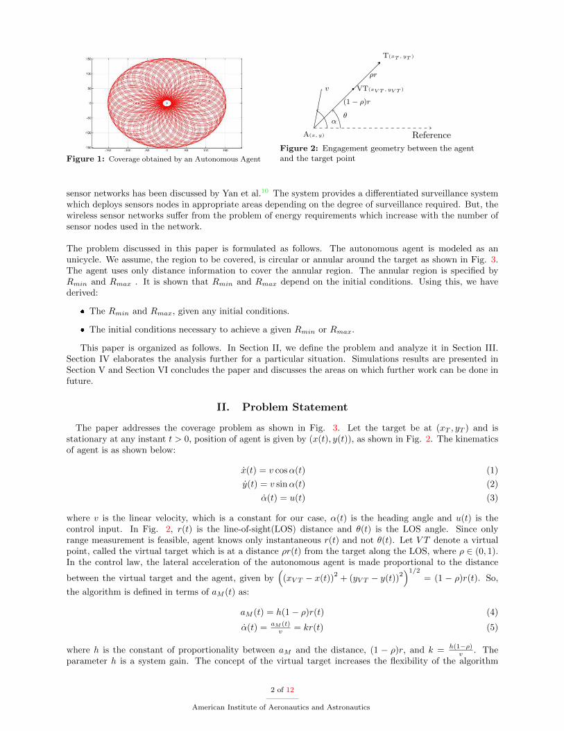
Figure 1: Coverage obtained by an Autonomous Agent

Reference

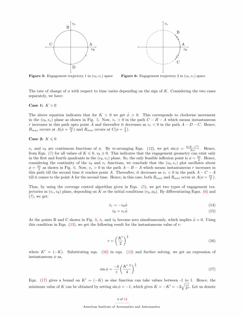
v

A(x, y)

θα

T(xT , yT )

VT(xV T , yV T )

(1− ρ)r

ρr

Figure 2: Engagement geometry between the agentand the target point

sensor networks has been discussed by Yan et al.10 The system provides a differentiated surveillance systemwhich deploys sensors nodes in appropriate areas depending on the degree of surveillance required. But, thewireless sensor networks suffer from the problem of energy requirements which increase with the number ofsensor nodes used in the network.

The problem discussed in this paper is formulated as follows. The autonomous agent is modeled as anunicycle. We assume, the region to be covered, is circular or annular around the target as shown in Fig. 3.The agent uses only distance information to cover the annular region. The annular region is specified byRmin and Rmax . It is shown that Rmin and Rmax depend on the initial conditions. Using this, we havederived:

� The Rmin and Rmax, given any initial conditions.

� The initial conditions necessary to achieve a given Rmin or Rmax.

This paper is organized as follows. In Section II, we define the problem and analyze it in Section III.Section IV elaborates the analysis further for a particular situation. Simulations results are presented inSection V and Section VI concludes the paper and discusses the areas on which further work can be done infuture.

II. Problem Statement

The paper addresses the coverage problem as shown in Fig. 3. Let the target be at (xT , yT ) and isstationary at any instant t > 0, position of agent is given by (x(t), y(t)), as shown in Fig. 2. The kinematicsof agent is as shown below:

x(t) = v cosα(t) (1)

y(t) = v sinα(t) (2)

α(t) = u(t) (3)

where v is the linear velocity, which is a constant for our case, α(t) is the heading angle and u(t) is thecontrol input. In Fig. 2, r(t) is the line-of-sight(LOS) distance and θ(t) is the LOS angle. Since onlyrange measurement is feasible, agent knows only instantaneous r(t) and not θ(t). Let V T denote a virtualpoint, called the virtual target which is at a distance ρr(t) from the target along the LOS, where ρ ∈ (0, 1).In the control law, the lateral acceleration of the autonomous agent is made proportional to the distance

between the virtual target and the agent, given by(

(xV T − x(t))2

+ (yV T − y(t))2)1/2

= (1 − ρ)r(t). So,

the algorithm is defined in terms of aM (t) as:

aM (t) = h(1− ρ)r(t) (4)

α(t) = aM (t)v = kr(t) (5)

where h is the constant of proportionality between aM and the distance, (1 − ρ)r, and k = h(1−ρ)v . The

parameter h is a system gain. The concept of the virtual target increases the flexibility of the algorithm

2 of 12


Rmax

Rmin

T

Figure 3: Region to be covered

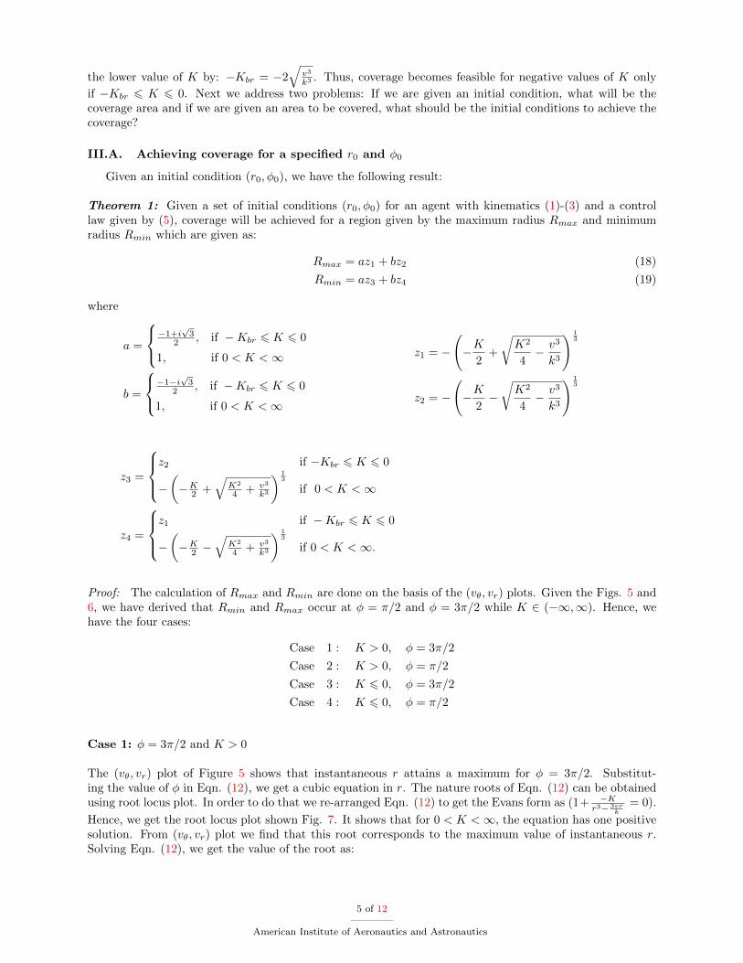
vθ

vr

A(φ = 3π2

)C(φ = π2

)

B(φ = π)

D(φ = 0)

Figure 4: (vθ, vr) plot

as we get another parameter ρ to be varied as needed. The algorithm generates various coverage patternssurrounding the stationary target. One of the patterns generated is shown in Fig. 1. In the next section,the control algorithm is analysed for area coverage applications.

III. Analysis

Consider the Fig. 2, the LOS between the agent and the target can be charaterised as follows:

vr = r = −v cos(α− θ) (6)

vθ = rθ = −v sin(α− θ) (7)

Let, φ = α− θ. From eqns. (5)-(7), we get,

φ = α− θ = kr +v sinφ

r(8)

From eqns. (6) and (8),

(kr2 − vθ)dr + vr cos(φ)dφ = 0 (9)

Solving the integration, we establish a relationship between r and φ as,

vr sinφ+kr3

3= vr0 sinφ0 +

kr30

3(10)

In the above equation, r0 and φ0 are the initial conditions. We define a variable K which contains all theterms corresponding to the initial conditions, such that,

K =

(3vr0 sin(φ0)

k+ r3

0

)(11)

Hence, Eqn. (10) can be re-written as:

r3 +3vr sinφ

k−K = 0 (12)

By setting Egn. (6) to zero, we observe that r can take its maximum and minimum values that is Rminand Rmax when φ equals either 3π

2 or π2 . Next we look into how the kinematics varies in the (vθ, vr) plane.

Upon squaring and adding Eqn. (6) and Eqn. (7), we find that the instantaneous vθ and vr lie on a circlein the (vθ, vr) plane as shown in Fig. 4. By the use of Eqns. (6) and (7), we can calculate the value of φcorresponding to each set of instantaneous vr and vθ. Point A corresponds to (vθ, vr) = (v, 0), thus, φ = 3π

2 .Similarly, we get that at B, φ = π, at C, φ = π

2 and at D, φ = 0. Hence, the clockwise movement about thecircle shown in Fig. 4 gives the direction of increasing values φ. Combining Eqns. (8) and (12), we get,

dφ

dt=k(K + 2r3)

3r2(13)

3 of 12


vθ

vr

C

B

A

D

Figure 5: Engagement trajectory 1 in (vθ, vr) space

vθ

vr

B

A

C

Figure 6: Engagement trajectory 2 in (vθ, vr) space

The rate of change of φ with respect to time varies depending on the sign of K. Considering the two casesseparately, we have:

Case 1: K > 0

The above equation indicates that for K > 0 we get φ > 0. This corresponds to clockwise movementin the (vθ, vr) plane as shown in Fig. 5. Now, vr > 0 in the path C − B − A which means instantaneousr increases in this path upto point A and thereafter it decreases as vr < 0 in the path A −D − C. Hence,Rmax occurs at A(φ = 3π

2 ) and Rmin occurs at C(φ = π2 ).

Case 2: K 6 0

vr and vθ are continuous functions of φ. By re-arranging Eqn. (12), we get sinφ = k(K−r3)3vr . Hence,

from Eqn. (7) for all values of K 6 0, vθ > 0. This indicates that the engagement geometry can exist onlyin the first and fourth quadrants in the (vθ, vr) plane. So, the only feasible inflexion point is φ = 3π

2 . Hence,considering the continuity of the vθ and vr functions, we conclude that the (vθ, vr) plot oscillates aboutφ = 3π

2 as shown in Fig. 6. Now, vr > 0 in the path A − B − A which means instantaneous r increases inthis path till the second time it reaches point A. Thereafter, it decreases as vr < 0 in the path A − C − Atill it comes to the point A for the second time. Hence, in this case, both Rmax and Rmin occur at A(φ = 3π

2 ).

Thus, by using the coverage control algorithm given in Eqn. (5), we get two types of engagement tra-jectories in (vr, vθ) plane, depending on K or the initial conditions (r0, φ0). By differentiating Eqns. (6) and(7), we get:

vr = −vθφ (14)

vθ = vrφ (15)

At the points B and C shown in Fig. 6, vr and vθ become zero simultaneously, which implies φ = 0. Usingthis condition in Eqn. (13), we get the following result for the instantaneous value of r:

r =

(K ′

2

) 13

(16)

where K ′ = (−K). Substituting eqn. (16) in eqn. (12) and further solving, we get an expression ofinstantaneous φ as,

sinφ =−kv

(K ′ 2

4

) 13

(17)

Eqn. (17) gives a bound on K ′ = (−K) as sine function can take values between -1 to 1. Hence, the

minimum value of K can be obtained by setting sinφ = −1, which gives K = −K ′ = −2√

v3

k3 . Let us denote

4 of 12


the lower value of K by: −Kbr = −2√

v3

k3 . Thus, coverage becomes feasible for negative values of K only

if −Kbr 6 K 6 0. Next we address two problems: If we are given an initial condition, what will be thecoverage area and if we are given an area to be covered, what should be the initial conditions to achieve thecoverage?

III.A. Achieving coverage for a specified r0 and φ0

Given an initial condition (r0, φ0), we have the following result:

Theorem 1: Given a set of initial conditions (r0, φ0) for an agent with kinematics (1)-(3) and a controllaw given by (5), coverage will be achieved for a region given by the maximum radius Rmax and minimumradius Rmin which are given as:

Rmax = az1 + bz2 (18)

Rmin = az3 + bz4 (19)

where

a =

−1+i√

32 , if −Kbr 6 K 6 0

1, if 0 < K <∞

b =

−1−i√

32 , if −Kbr 6 K 6 0

1, if 0 < K <∞

z1 = −

(−K

2+

√K2

4− v3

k3

) 13

z2 = −

(−K

2−√K2

4− v3

k3

) 13

z3 =

z2 if −Kbr 6 K 6 0

−(−K2 +

√K2

4 + v3

k3

) 13

if 0 < K <∞

z4 =

z1 if −Kbr 6 K 6 0

−(−K2 −

√K2

4 + v3

k3

) 13

if 0 < K <∞.

Proof: The calculation of Rmax and Rmin are done on the basis of the (vθ, vr) plots. Given the Figs. 5 and6, we have derived that Rmin and Rmax occur at φ = π/2 and φ = 3π/2 while K ∈ (−∞,∞). Hence, wehave the four cases:

Case 1 : K > 0, φ = 3π/2

Case 2 : K > 0, φ = π/2

Case 3 : K 6 0, φ = 3π/2

Case 4 : K 6 0, φ = π/2

Case 1: φ = 3π/2 and K > 0

The (vθ, vr) plot of Figure 5 shows that instantaneous r attains a maximum for φ = 3π/2. Substitut-ing the value of φ in Eqn. (12), we get a cubic equation in r. The nature roots of Eqn. (12) can be obtainedusing root locus plot. In order to do that we re-arranged Eqn. (12) to get the Evans form as (1+ −K

r3− 3vrk

= 0).

Hence, we get the root locus plot shown Fig. 7. It shows that for 0 < K <∞, the equation has one positivesolution. From (vθ, vr) plot we find that this root corresponds to the maximum value of instantaneous r.Solving Eqn. (12), we get the value of the root as:

5 of 12


Figure 7: Root Locus for positive K and φ = 3π/2 Figure 8: Root Locus for positive K and φ = π/2

Rmax = −

(−K

2+

√K2

4− v3

k3

) 13

−

(−K

2−√K2

4− v3

k3

) 13

(20)

Case 2: φ = π/2 and K > 0

Proceeding the same way as for the previous case, we conclude that for K > 0, φ = π2 corresponds to

the minimum value of the instantaneous r. Hence, by substituting this condition in Eqn. (12), we get acubic equation in r. To analyse the behaviour of the roots, we re-arrange Eqn. (12), to get the Evan’s formas (1 + −K

r3+ 3vrk

= 0). The root locus plot of the equation is given in Fig. 8. It shows that for 0 < K < ∞,

the equation has one positive solution which corresponds to the minimum value of instantaneous r. SolvingEqn. (12), we get the value of the root as:

Rmin = −

(−K

2+

√K2

4+v3

k3

) 13

−

(−K

2−√K2

4+v3

k3

) 13

(21)

Case 3: φ = 3π/2 and K 6 0

The (vθ, vr) plot of Fig. (6) shows that for φ = 3π/2, the instantaneous r attains both its maximum andminimum values in an alternate manner. Substituting the value of φ in Eqn. (12), we get the cubic equation

in terms of r. To generate the root locus, we re-arranged Eqn. (12) to get the Evans form as (1+ K′

r3− 3vrk

= 0),

where K ′ = −K. The root locus plot, shown in Fig. 9, shows that for 0 6 K ′ 6 Kbr, the equation yields twopositive roots indicating Rmax and Rmin. But, beyond K ′ = Kbr which corresponds to the breakaway valueof K ′, the two positive roots become imaginary. Hence, no value of K ′ greater than Kbr gives a feasiblesolution. At the breakaway value of K ′ = Kbr = 2( vk )

32 , Rmax and Rmin become equal. Now, before solving

the eqn. (12), we define two terms z1 = −(−K2 +

√K2

4 −v3

k3

) 13

and z2 = −(−K2 −

√K2

4 −v3

k3

) 13

. The

instantaneous value of r corresponding to its maximum and minimum values are given by,

Rmax =

(−1 + i

√3

2

)z1 +

(−1− i

√3

2

)z2 (22)

Rmin =

(−1− i

√3

2

)z1 +

(−1 + i

√3

2

)z2 (23)

6 of 12


Figure 9: Root Locus for negative K and φ = 3π/2 Figure 10: Root Locus for negative K and φ = π/2

Case 4: φ = π/2 and K 6 0

We substituted these values in Eqn. (12) to get the Evans form as (1 + K′

r3+ 3vrk

= 0). By using the Evans

form, we obtained the root locus plot as shown in Fig. 10. It shows that, no feasible roots exist. Hence,coverage cannot be attained for this configuration.

Hence, we can conclude from the four cases that given an initial condition, the maximum and minimumradii of the annular region that can be covered by the agent is as given in Eqns. (20), (21), (22) and (23). 2

III.B. Achieving coverage with desired Rmax and Rmin

In the previous section, we saw that for any initial condition, we can calculate the value of K. Usingthat K value, we can obtain the maximum and minimum value that the instantaneous r can take. Now,if the user specifies the Rmax and Rmin values, it is possible to generate the initial conditions a priori byperforming some calculations. But, as for the algorithm, Rmax and Rmin are always dependent on eachother. So, once Rmax is specified by the user, then, Rmin can take only specific values. The relationshipexisting between Rmax and Rmin can be established as follows: For any K satisfying −Kbr 6 K 6 0, φ = 3π

2gives both Rmax and Rmin. So, replacing r by Rmax or Rmin and the corresponding value of φ = 3π

2 in Eqn.

(12) gives, K = R3min− 3vRmin

k = R3max− 3vRmax

k . For any value of K such that 0 < K <∞, by performing

similar calculations, we get, K = R3min + 3vRmin

k = R3max − 3vRmax

k . Hence, given desired Rmax or Rmin,then the parameter K can be evaluated. Eqn. (11) can be re-arranged to get,

sinφ0 =k(K − r3

0)

3vr0(24)

Case 1: 0 < K <∞

From the (vθ, vr), shown in Figure 5, we know that for 0 < K < ∞, −v < vθ < v which implies−1 < − sinφ0 < 1 and φ0 ∈ (0, 2π). Hence, by using (24), we get the range of feasible values of r0

given by,

− 1 <k(K − r3

0)

3vr0< 1 (25)

Case 2:−Kbr 6 K 6 0

For this case, we get the (vθ, vr) as shown in Figure 6. This indicates 0 6 vθ 6 1 which implies −1 6− sinφ0 6 0 and π ∈ [π, 2π]. So, combining this result with Eqn. (24), we get,

− 1 6k(K − r3

0)

3vr06 0 (26)

Hence, for any r0 = r0, chosen from the range of values obtained from either Eqn. (25) or eqn. (26), the

appropriate value of φ0 = φ0 can be calculated from Eqn.(24) i.e. sin φ0 = k(K−r03)3vr0

. Hence, for each value

7 of 12


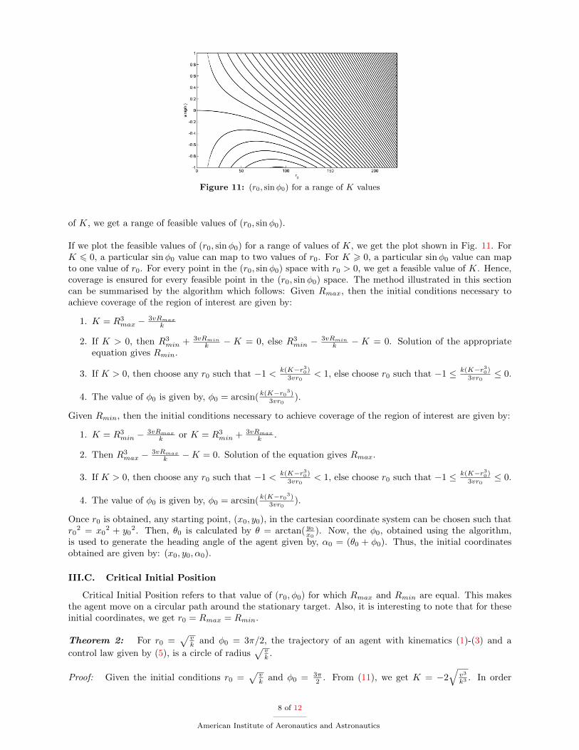
Figure 11: (r0, sinφ0) for a range of K values

of K, we get a range of feasible values of (r0, sinφ0).

If we plot the feasible values of (r0, sinφ0) for a range of values of K, we get the plot shown in Fig. 11. ForK 6 0, a particular sinφ0 value can map to two values of r0. For K > 0, a particular sinφ0 value can mapto one value of r0. For every point in the (r0, sinφ0) space with r0 > 0, we get a feasible value of K. Hence,coverage is ensured for every feasible point in the (r0, sinφ0) space. The method illustrated in this sectioncan be summarised by the algorithm which follows: Given Rmax, then the initial conditions necessary toachieve coverage of the region of interest are given by:

1. K = R3max − 3vRmax

k

2. If K > 0, then R3min + 3vRmin

k − K = 0, else R3min − 3vRmin

k − K = 0. Solution of the appropriateequation gives Rmin.

3. If K > 0, then choose any r0 such that −1 <k(K−r30)

3vr0< 1, else choose r0 such that −1 ≤ k(K−r30)

3vr0≤ 0.

4. The value of φ0 is given by, φ0 = arcsin(k(K−r03)3vr0

).

Given Rmin, then the initial conditions necessary to achieve coverage of the region of interest are given by:

1. K = R3min − 3vRmax

k or K = R3min + 3vRmax

k .

2. Then R3max − 3vRmax

k −K = 0. Solution of the equation gives Rmax.

3. If K > 0, then choose any r0 such that −1 <k(K−r30)

3vr0< 1, else choose r0 such that −1 ≤ k(K−r30)

3vr0≤ 0.

4. The value of φ0 is given by, φ0 = arcsin(k(K−r03)3vr0

).

Once r0 is obtained, any starting point, (x0, y0), in the cartesian coordinate system can be chosen such thatr0

2 = x02 + y0

2. Then, θ0 is calculated by θ = arctan( y0x0). Now, the φ0, obtained using the algorithm,

is used to generate the heading angle of the agent given by, α0 = (θ0 + φ0). Thus, the initial coordinatesobtained are given by: (x0, y0, α0).

III.C. Critical Initial Position

Critical Initial Position refers to that value of (r0, φ0) for which Rmax and Rmin are equal. This makesthe agent move on a circular path around the stationary target. Also, it is interesting to note that for theseinitial coordinates, we get r0 = Rmax = Rmin.

Theorem 2: For r0 =√

vk and φ0 = 3π/2, the trajectory of an agent with kinematics (1)-(3) and a

control law given by (5), is a circle of radius√

vk .

Proof: Given the initial conditions r0 =√

vk and φ0 = 3π

2 . From (11), we get K = −2√

v3

k3 . In order

8 of 12


to calculate the Rmax and Rmin using the K and φ0 values, we refer to Theorem 1. Since K ∈ [−Kbr, 0],

from case III of theorem, we get that K = −2√

v3

k3 corresponds to the breakaway point of the root locus

given in Fig. 9. At the breakaway point, two roots of the Eqn. (12) are real and equal and the third root isimaginary, as shown in Fig. 9. Hence, by using Eqns. (22) and (23) for the given initial conditions, we getRmax and Rmin as:

Rmax = Rmin =

√v

k(27)

The given initial conditions, which make the agent circle around the stationary target, are referred to as thecritical initial position, given by,

r0 = rcr =

√v

k

sinφ0 = −1⇒ φ0 = 3π/2(28)

From (27) and (28), we conclude that r0 = Rmax = Rmin. Hence, the autonomous agent circles around thetarget with a fixed radius of

√vk for all time t > 0. 2

IV. Special case: Behaviour of the system when φ0 = 3π/2

The coverage algorithm, designed here, ensures coverage for all feasible values of initial radial distance, r0

and φ0. But, the particular situation of φ0 = 3π/2 gives interesting results for Rmax and Rmin. Also, in theprevious section, we saw that for φ0 = 3π/2 the agent revolves around the target with a radius r =

√vk .

Now, we have K =(r30 − 3vr0

k

). Hence, for 0 6 r0 6

√3vk , we get K 6 0 and for r0 >

√3vk , we get K > 0.

IV.A. Maximum & Minimum radii for any initial radial distance, r0

In this section, we have derived the Rmax and Rmin for φ0 = 3π2 . The Rmax and Rmin follow patterns

as we vary the initial radial distance r0.

Case 1: K 6 0

From the (vθ, vr) plot of Fig. 6, we get φ = 3π2 corresponds to both Rmax and Rmin. Simplifying the

eqns. (22) and (23) yields two positive roots, Rmax and Rmin:

r1 = r0 (29)

r2 =−r0 +

√−3r2

0 − 4 12vk

2(30)

Now, depending on r0, one of the roots becomes Rmax and the other Rmin. For initial radial distanceless than r0 = rcr , r = r0 becomes Rmin and the other root becomes Rmax which exactly reverses for

rcr ≤ r0 ≤√

3vk . So, the behaviour of the Rmax and Rmin vary in accordance to the initial radial distance

from the target.

Case 2: K > 0

The (vθ, vr) plot of Figure 5 gives φ = 3π2 indicates Rmax and φ = π

2 indicates Rmin. Simplifying theEqns. (20) and (21), we get the two positive roots as:

Rmax = r0 (31)

Rmin = −

(K

2+

√K2

4+v3

k3

) 13

−

(K

2−√K2

4+v3

k3

) 13

(32)

All the above results were verified from their second derivatives.

9 of 12


Figure 12: Rmax for φ = 3π/2, 0 < r0 <√vk

Figure 13: Rmax for φ = 3π/2,√vk < r0 <

√3vk

Figure 14: Rmin for φ = 3π/2 and 0 < r0 <√vk

Figure 15: Rmin for φ = 3π/2 and√vk < r0 <

√3vk

IV.B. Agent restricts itself within a stretch of radius√

3vk

Given, φ0 = 3π2 , the trajectory of the agent has a peculiar behaviour: For 0 6 r0 6

√3vk , the maximum

radial distance that can be covered by the agent can reach a maximum of Rmax =√

3vk and never exceed

it. In a similar manner, the minimum radius that the agent can reach is Rmin = 0.

Corollary 1: Given φ0 = 3π2 , for any initial position r0 ∈

[0,√

3vk

], the trajectory of the agent is bound

by a circle of radius√

3vk .

Proof: In the previous section, we derived the values of Rmax and Rmin for any arbitrary initial posi-tion r0. Eqns. (29) and (30) establish a relationship of Rmax and Rmin with r0. The nature of the variationRmax and Rmin with respect to r0 can be explained by plotting (29) and (30). Fig. 12 shows the variation

of Rmax for r0 ∈[0,√

vk

]and Fig. 13 shows the same for r0 ∈

[√vk ,√

3vk

].

For r0 ∈[0,√

vk

], Fig. 14 shows variation of Rmin with respect to r0 and Fig. 15 shows variation of

Rmin for r0 ∈[√

vk ,√

3vk

]. From the plots, it is clear that max(Rmax =

√3vk ) and min(Rmin) = 0.This

ensures that if the agent starts with φ0 = 3π/2, then for any value of r0, the agent will always remain within

a circle of radius r =√

3vk . 2

For the particular case of r0 = 0 and φ0 = 3π2 , since r0 ∈ [0,

√vk ] we refer to Eqn. (29), to get Rmax =

√3vk

and Rmin = 0. This makes the agent cover the entire area of the circle of radius√

3vk centred around the

stationary target.

V. Simulation Results

In this section, we validate the results obtained in sections III and IV through MATLAB simulations.The simulations were performed with the parameters h = 0.01, ρ = 0.3 and v = 5. The control algorithmdeveloped in Eqn. (5) leads to formation of patterns around the target ensuring coverage of the area

10 of 12


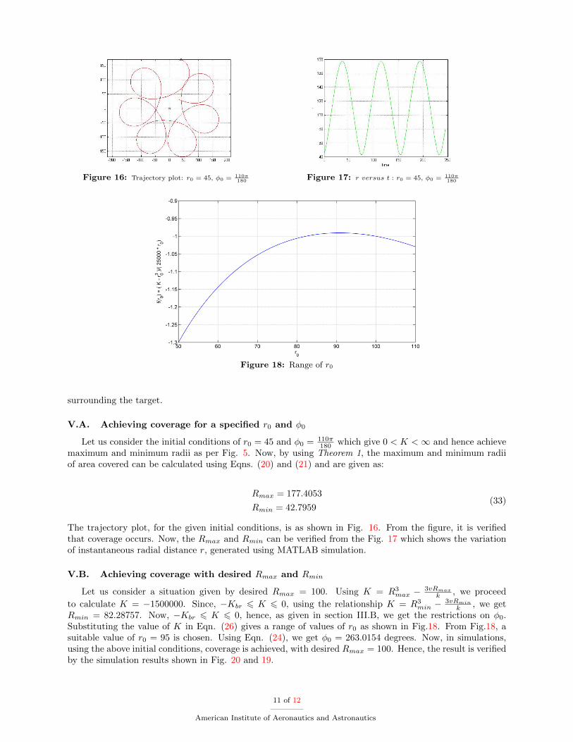
Figure 16: Trajectory plot: r0 = 45, φ0 = 110π180 Figure 17: r versus t : r0 = 45, φ0 = 110π

180

Figure 18: Range of r0

surrounding the target.

V.A. Achieving coverage for a specified r0 and φ0

Let us consider the initial conditions of r0 = 45 and φ0 = 110π180 which give 0 < K <∞ and hence achieve

maximum and minimum radii as per Fig. 5. Now, by using Theorem 1, the maximum and minimum radiiof area covered can be calculated using Eqns. (20) and (21) and are given as:

Rmax = 177.4053

Rmin = 42.7959(33)

The trajectory plot, for the given initial conditions, is as shown in Fig. 16. From the figure, it is verifiedthat coverage occurs. Now, the Rmax and Rmin can be verified from the Fig. 17 which shows the variationof instantaneous radial distance r, generated using MATLAB simulation.

V.B. Achieving coverage with desired Rmax and Rmin

Let us consider a situation given by desired Rmax = 100. Using K = R3max − 3vRmax

k , we proceed

to calculate K = −1500000. Since, −Kbr 6 K 6 0, using the relationship K = R3min − 3vRmin

k , we getRmin = 82.28757. Now, −Kbr 6 K 6 0, hence, as given in section III.B, we get the restrictions on φ0.Substituting the value of K in Eqn. (26) gives a range of values of r0 as shown in Fig.18. From Fig.18, asuitable value of r0 = 95 is chosen. Using Eqn. (24), we get φ0 = 263.0154 degrees. Now, in simulations,using the above initial conditions, coverage is achieved, with desired Rmax = 100. Hence, the result is verifiedby the simulation results shown in Fig. 20 and 19.

11 of 12


Figure 19: Trajectory plot: for r0 = 95, φ0 = 263.0154 Figure 20: r versus t : r0 = 95, φ0 = 263.0154

VI. Conclusion

In the paper, we presented a strategy that can make an autonomous agent cover the region surrounding astationary target, using only range measurement. We derived the Rmax and Rmin values which characterisethe region covered by the autonomous agent under the control law (5), given any initial conditions(r0, φ0).Similarly, we derived the initial conditions necessary to cover the region-of-interest when Rmax and Rminare given. We also showed that under certain initial conditions, the agent covers the area around the targetby revolving around the stationary target on a circle of fixed radius. The radius of the circular trajectorydepends on the fixed parameters involved in the system of equations and, hence, can be specified by theuser. As the guidance strategy uses only range measurement to achieve coverage, the energy requirements ofthe entire system are minimised. In the paper, the effect of initial conditions on the pattern generation hasbeen studied. The work can be extended to study the effect of system parameters, like ρ, on the patternsgenerated. Further work can also be done to calculate the time required to cover the area specified by theuser.

References

1S. C. Wong, B. A. MacDonald, “A topological coverage algorithm for mobile robots,” Proceedings of the IEEW/RSJInternational Conference on Intelligent Robots and Systems, Vol. 2, 1685-1690, 2003.

2A. Zelinsky , R.A. Jarvis , J. C. Byrne , S. Yuta., “Planning paths of complete coverage of an unstructured environmentby a mobile robots,” Proceedings of International Conference on Advanced Robotics, 533-538, 1993.

3C. Stachniss and W. Burgard, “Mapping and Exploration with Mobile Robots using Coverage Maps,” Proceedings ofthe IEEW/RSJ International Conference on Intelligent Robots and Systems, Vol. 1, 1127-1132, 2003.

4S. Rutishauser , N. Correll and A. Martinoli, “Collaborative coverage using a swarm of networked miniature robots,”Robotics and Autonomous Systems, Vol. 57, 517-525, 2009.

5P. H. Batavia, S. A. Roth, S. Singh, “Autonomous Coverage Operations In Semi-Structured Outdoor Environments,”Proceedings of the IEEW/RSJ International Conference on Intelligent Robots and Systems, 743-749, 2002.

6Ercan U. Acar, Howie Choset and Prasad N. Atkar, “Complete Sensor-based Coverage with Extended-range Detectors:A Hierarchical Decomposition in Terms of Critical Points and Voronoi Diagrams,” Proceedings of the IEEW/RSJ InternationalConference on Intelligent Robots and Systems, 1305-1311, 2001

7S. S. Dhillon and K. Chakrabarty, “Sensor Placement for Effective Coverage and Surveillance in Distributed SensorNetworks,”Proceedings of IEEE Wireless Communications and Networking Conference, 1609-1614, 2003.

8Chih-Chung Lai, Chuan-Kang Ting and Ren-Song Ko, “An Effective Genetic Algorithm to Improve Wireless SensorNetwork Lifetime for Large-Scale Surveillance Applications,” IEEE Congress on Evolutionary Computation, 3531-3538, 2007.

9Wei Wang, Vikram Srinivasan, Bang Wang, and Kee-Chaing Chua, “Coverage for Target Localization in Wireless SensorNetworks,” IEEE Transactions on Wireless Communications, Vol. 7, No. 2, 667-676, 2008.

10Ting Yan, Tian He and John A. Stankovic, “Differentiated Surveillance for Sensor Networks,” First ACM Conferenceon Embedded Networked Sensor Systems, 51-62, 2003.

12 of 12


guidance of an autonomous agent for coverage applications

Documents