guidance on applying the monte carlo approach … · carlo approach to uncertainty analyses in...

Anna McMurray, Timothy Pearson and Felipe Casarim 2017

GUIDANCE ON APPLYING THE MONTE CARLO APPROACH TO UNCERTAINTY

ANALYSES IN FORESTRY AND GREENHOUSE GAS ACCOUNTING

Guidance on Applying the Monte Carlo Approach | 2017

Guidance on Applying the Monte Carlo Approach 2017

Contents

1. Introduction ................................................................................................................................................... 4

2. Monte Carlo simulation approach................................................................................................................ 5

3. Steps to carry out uncertainty analyses using Monte Carlo ....................................................................... 7 3.1 Fitting distributions .......................................................................................................................................................................... 7

Identifying PDFs when entire data set is available........................................................................................................................................ 7 Identifying PDFs when underlying distribution is not available ................................................................................................................... 10

3.2 Running Monte Carlo simulations ................................................................................................................................................ 11 Selecting software ..................................................................................................................................................................................... 11 Developing simulations ............................................................................................................................................................................. 12 Truncation of fitted distribution ................................................................................................................................................................ 12

3.3 Combining Monte Carlo simulations ........................................................................................................................................... 13 3.4 Calculating confidence intervals ................................................................................................................................................... 15

Confidence intervals for normal distributions .............................................................................................................................................. 15 Confidence intervals for non-normal distributions ........................................................................................................................................ 15

3.5 Calculating percent uncertainty ..................................................................................................................................................... 17

4. Full application of the Monte Carlo approach ........................................................................................... 18

5. Discussion on applying Monte Carlo to uncertainty analyses .................................................................. 18

Annex ..................................................................................................................................................................... 20 4 Annex 1: Simplified example of application of the Monte Carlo approach ............................................................................. 20

A. Fitting distributions and running the Monte Carlo simulations .......................................................................................................... 20 B. Applying Monte Carlo simulations to equations to calculate uncertainty of total emissions ................................................................... 23 C. Calculating the confidence interval .................................................................................................................................................... 25 D. Calculating uncertainty ................................................................................................................................................................... 26



Figures Figure 1. Examples of commonly used probability density function models (taken from Figure 3.5 of the IPCC) ..... 6

Figure 2. Illustration of the Monte Carlo approach ............................................................................................................ 6

Figure 3. Steps to carrying out the Monte Carlo approach to calculating uncertainty ..................................................... 7

Figure 4. Illustration of outlier data ...................................................................................................................................... 8

Figure 5. Example of a PDF fit to a dataset ........................................................................................................................ 9

Figure 6. Simulation using normal distribution with and without truncation. ................................................................ 13

Figure 7. Simulation using lognormal distribution with and without truncation. ........................................................... 13

Figure 8. Example of application of Monte Carlo simulations to model estimating total emissions ............................ 14

Figure 9. Median values of a population are resampled 1,000 times, using the bootstrapping technique .................... 16

Figure 10. Confidence interval calculated through the bootstrapping method is the difference between the 2.5th percentile and 97.5th percentile of the bootstrapped distribution of medians ............................................................... 17

Figure 11. Examples of using quantiles of final emission distribution to calculate uncertainty .................................... 19

This project is part of the International Climate Initiative (IKI). The German Federal Ministry for the Environment, Nature Conservation, Building and Nuclear Safety (BMUB) supports this initiative on the basis of a decision adopted by the German Bundestag.

For comments or questions please contact the lead author: Anna McMurray: [email protected]

mailto:[email protected]?subject=Re:%20Guidance%20Document%20on%20Uncertainty%20Analyses



1. Introduction When calculating greenhouse gas emissions, it is always necessary to evaluate and quantify the uncertainties of the estimates. Uncertainty analyses help analysts and decision makers identify how accurate the estimations are and the likely range in which the true value of the emissions fall. There are three general steps in performing any uncertainty analysis: 1) Identifying the sources of uncertainty in the estimate; 2) quantifying the different sources of uncertainty, whenever possible; and 3) combining/aggregating the different uncertainties to come up with a final uncertainty value. Chapter 3 of the 2006 IPCC Guidelines for National Greenhouse Gas Inventories Volume 11 (hereinafter, referred to as the IPCC) provides information on uncertainty analysis methods. To perform the third step of uncertainty analyses, the combination of uncertainties, the IPCC presents two approaches:

1) Propagation of error, and

2) Monte Carlo simulation.

Propagation of error involves combining uncertainty estimates in simple equations. It is considered a Tier 1 approach and can be applied by almost anyone with experience in using equations in spreadsheets. The Monte Carlo simulation approach is significantly more complex in that it involves the repeated generation of random values, based on the distributions of the input data. Because of the higher complexity level, analysts without significant statistical background will need detailed guidance on how to carry out Monte Carlo simulations. However, for anything beyond the most basic uncertainty analyses Monte Carlo simulations are highly preferable. A propagation of errors approach is not appropriate under the following circumstances, as noted in the IPCC:

• Uncertainty is large2;

• Distributions are not normal;

• Equations are complex;

• Data are correlated;

• Different uncertainties in different inventory years

It is therefore important to be cognizant that in most forestry and greenhouse gas accounting contexts there will be large uncertainty in the input data, distributions will often be non-normal, equations can be complex, between many datasets correlations do exist and annual variation is significant in any natural system. Thus, Monte Carlo is the correct approach. and use of Monte Carlo uncertainty analyses must grow more prevalent.

1 Frey, C., Penman, J., Hanle, L., Monni, S., Ogle, S. (2006). Chapter 3. Uncertainties. In Volume 1, General Guidance and Reporting, 2006 IPCC Guidelines for National Greenhouse Gas Inventories, National Greenhouse Gas Inventories Programme (pp. 66). Kanagawa, Japan. Inter-Governmental Panel on Climate Change, Technical Support Unit. https://www.ipcc-nggip.iges.or.jp/public/2006gl/vol1.html.

2 According to the IPCC, uncertainty is considered large when the standard deviation divided by the mean is greater than 0.3

https://www.ipcc-nggip.iges.or.jp/public/2006gl/vol1.html



The IPCC provides general information on the Monte Carlo simulation approach but limited information on how to implement it. Any application of running Monte Carlo simulations and applying the results to estimate uncertainty raises a series of questions and issues which are not addressed in the IPCC guidelines. This guidance aims to help fill the information gaps that currently exist and to serve as a technical guide for analysts who desire to apply the Monte Carlo approach to uncertainty analyses. It is assumed that the people using this guidance have the following:

• An understanding of descriptive statistics and some experience in the application of basic statistics (for example, the ability to carry out uncertainty analyses using propagation of error) but little experience applying the Monte Carlo approach in particular.

• Basic proficiency in using Excel (i.e., have familiarity with basic Excel functions and can create simple equations). Different Excel-based software recommendations are provided based on the authors’ own experience with them. However, the reader should investigate the best options available to him/her including other Excel-based programs. If the reader has proficiency in other statistical software, such as R, SAS, and SPSS, he/she should consider these options as well.

The guidance will focus on application to REDD+ analyses but could be potentially applied to uncertainty analyses of GHG emissions from other sectors or, more broadly, to any type of uncertainty analysis. A simple example of implementing the Monte Carlo approach to combining uncertainties is provided in Annex 1.

2. Monte Carlo simulation approach The Monte Carlo approach involves the repeated simulation of samples within the probability density functions of the input data (e.g.., the emission or removal factors, and activity data). Probability density functions (PDFs) explain the range of potential values of a given variable and the likelihood that different values represent the true value. PDFs are graphically represented as distributions. Common examples include normal (Gaussian) distributions, lognormal, triangular, and uniform, as shown in Figure 1 (taken from the IPCC).



UNIFORM TRIANGULAR NORMAL LOGNORMAL

Figure 1. Examples of commonly used probability density function models (taken from Figure 3.5 of the IPCC)

The Monte Carlo simulations are run using algorithms which generate stochastic (i.e., random) values based on the PDF of the data. The objective of these repeated simulations is to produce distributions that represent the likelihood of different estimates. Once the simulations have been run, they are applied to the model, which could be complex or be a simple equation, developed to calculate the final estimate. To calculate the uncertainty, the confidence interval can then be identified for the final distributions, as show in Figure 2. In the context of measuring uncertainty of emission reductions, Monte Carlo simulations are run for all data inputs (i.e., emission factor and activity data) identified as sources of uncertainty. The resulting simulations would then be applied to equations used to estimate the emission reductions, as shown in Figure 8 in Section 3.3.

Figure 2. Illustration of the Monte Carlo approach



3. Steps to carry out uncertainty analyses using Monte Carlo Once the different sources of uncertainty have been identified and quantified when possible, the Monte Carlo approach can be implemented through 5 major steps as shown in Figure 3 and discussed in detail in the following sections.

Figure 3. Steps to carry out the Monte Carlo approach for calculating uncertainty

3.1 Fitting distributions Before running Monte Carlo simulations, it is necessary to identify the probability density functions (PDFs) that have a good fit with each of the data sources with key uncertainty sources identified.

Identifying PDFs when entire data set is available Ideally, the entire dataset is available to identify its distribution and the database is derived from a random sample that is representative of the underlying population. When the entire dataset is available, the analysts should adjust the data to account for any known biases in the data or outlier values. As defined in the IPCC, a bias, also referred to as a systematic error, is a lack of accuracy, i.e., lack of agreement between the true value and the average of repeated measured observations or estimates of the variable. Identifying and estimating biases will frequently require a good understanding of the system being analyzed. For example, if biomass field measurements could only be conducted in particularly dense forests as compared to the average forest within a given jurisdiction or country, then the analyst should adjust the emission factor estimates for deforestation downward to account for this bias based on expert judgment. For activity data, accuracy assessments can be performed such as the approach presented by Olofsson et al (2013)3 to identify and correct for major biases.

3 Olofsson, P., Foody, G. M., Stehman, S. V., & Woodcock, C. E. (2013). Making better use of accuracy data in land change studies: Estimating accuracy and area and quantifying uncertainty using stratified estimation. Remote Sensing of Environment, 129, 122-131.

1. FIT DISTRIBUTIONS TO INPUT DATA

2. RUN MONTE CARLO

SIMULATIONS

3. COMBINE MONTE CARLO SIMULATIONS

4. CALCULATE CONFIDENCE INTERVALS

5. CALCULATE %

UNCERTAINTY



Outlier values are data points that lie at an abnormal distance from the rest of the data set (Figure 4). These values can have a substantial impact on the overall shape of the data distribution and, therefore, the resulting probability distribution. Whether or not to remove outlier data is up to the discretion of the analyst based on his/her knowledge of the underlying data. Outlier values may be important components of the data set and, therefore, should not be removed. However, they may also represent measurement or recording error, in which case, they should be removed.

Figure 4. Illustration of outlier data

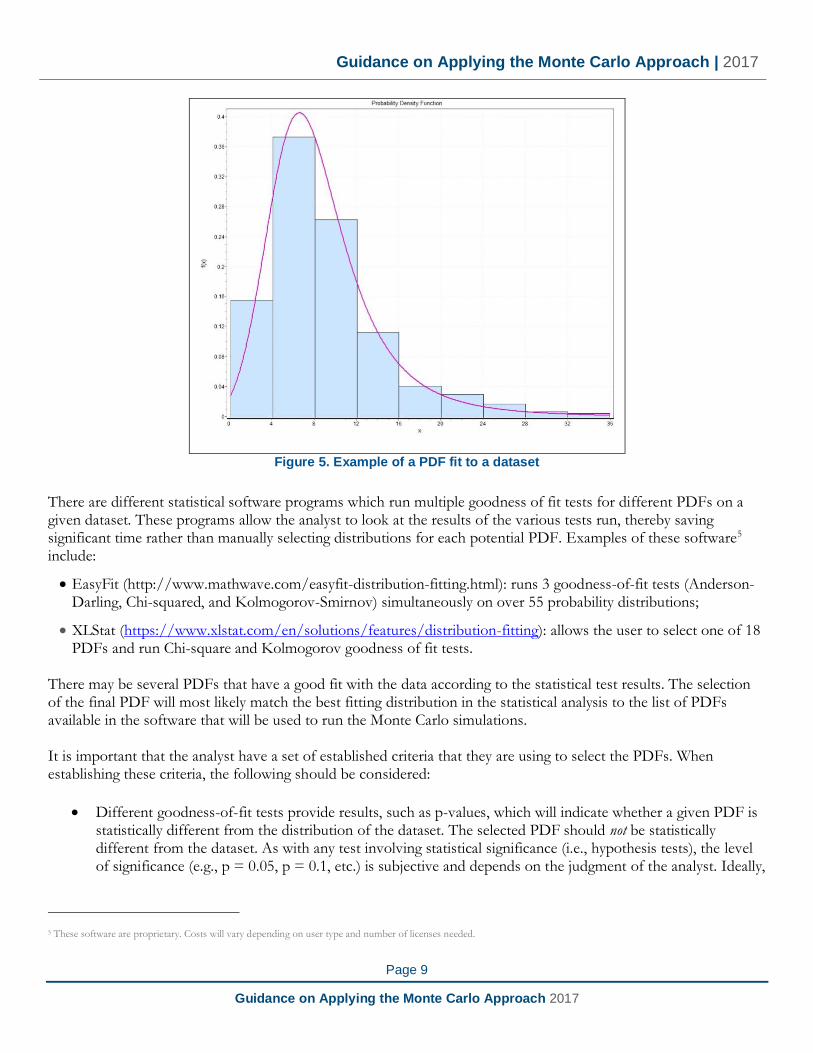
Once the data has been adjusted to account for biases and outliers, a variety of goodness-of-fit tests4 can be applied to identify the PDF best fit to the data. Figure 5 provides an example of fitting a PDF to data. In this case, the blue bars illustrate the distribution of the actual data and the purple line represents the PDF (Generalized Logistic) that was identified as having a good fit.

4 Goodness-of-fit tests include Shapiro-Wilks (only to test if distributions are normal or non-normal), Chi-squared, Kolmogorov-Smirnov, and Anderson-Darling. All of these tests require the identification of a particular PDF (e.g., normal, lognormal, uniform etc.) to test if the PDF fits the data.

OUTLIER VALUE



Figure 5. Example of a PDF fit to a dataset

There are different statistical software programs which run multiple goodness of fit tests for different PDFs on a given dataset. These programs allow the analyst to look at the results of the various tests run, thereby saving significant time rather than manually selecting distributions for each potential PDF. Examples of these software5 include:

• EasyFit (http://www.mathwave.com/easyfit-distribution-fitting.html): runs 3 goodness-of-fit tests (Anderson-Darling, Chi-squared, and Kolmogorov-Smirnov) simultaneously on over 55 probability distributions;

• XLStat (https://www.xlstat.com/en/solutions/features/distribution-fitting): allows the user to select one of 18 PDFs and run Chi-square and Kolmogorov goodness of fit tests.

There may be several PDFs that have a good fit with the data according to the statistical test results. The selection of the final PDF will most likely match the best fitting distribution in the statistical analysis to the list of PDFs available in the software that will be used to run the Monte Carlo simulations. It is important that the analyst have a set of established criteria that they are using to select the PDFs. When establishing these criteria, the following should be considered:

• Different goodness-of-fit tests provide results, such as p-values, which will indicate whether a given PDF is statistically different from the distribution of the dataset. The selected PDF should not be statistically different from the dataset. As with any test involving statistical significance (i.e., hypothesis tests), the level of significance (e.g., p = 0.05, p = 0.1, etc.) is subjective and depends on the judgment of the analyst. Ideally,

5 These software are proprietary. Costs will vary depending on user type and number of licenses needed.

https://www.xlstat.com/en/solutions/features/distribution-fitting



the final PDF selected should be the one deemed as having the best fit to the data set according to the statistical test results.

• Since Monte Carlo software provide limited options of PDFs, the final PDF selected should be one available in the software elected to run Monte Carlo, which ranks as having the best fit according to the statistical tests, and is not statistically significant from the data using the significance level threshold established by the analyst.

• If a normal (gaussian) distribution ranks among the best fitting statistically significant distributions, then it should be preferred.

The goodness of fit tests should provide parameters (for example, mean and standard deviation) of the selected PDF, which the analyst can then use to run Monte Carlo simulations. Before running the simulations, however, the analyst should ensure that the parameters are the same as those required to run the simulations. If not, they need to be converted to the parameters required for the simulations6.

Identifying PDFs when underlying distribution is not available When the entire dataset is unavailable, the analyst must rely on an understanding of the source of the underlying data as well as any available metrics (e.g., standard deviation, range, root mean square deviation, etc) associated with the estimated value. In Section 3.2.2.4., the IPCC provides circumstances for the use of various common PDFs including normal, lognormal, uniform, triangular, and fractile (Box 1).

Box 1.

Examples of common PDFs and the situations they represent (taken from Section 3.2.2.4 of the IPCC)

• The normal distribution is most appropriate when the range of uncertainty is small, and symmetric

relative to the mean. The normal distribution arises in situations where many individual inputs

contribute to an overall uncertainty, and in which none of the individual uncertainties dominates

the total uncertainty.

• Similarly, if an inventory is the sum of uncertainties of many individual categories, however, none of

which dominates the total uncertainty, then the overall uncertainty is likely to be normal. A

normality assumption is often appropriate for many categories for which the relative range of

uncertainty is small, e.g., fossil fuel emission factors and activity data.

• The lognormal distribution may be appropriate when uncertainties are large for a non-negative

variable and known to be positively skewed. The emission factor for nitrous oxide from fertiliser applied to soil provides a typical inventory example. If many uncertain variables are multiplied, the

product asymptotically approaches lognormality. Because concentrations are the result of mixing

processes, which are in turn multiplicative, concentration data tend to be distributed similar to a

6 For example, in the software EasyFit (http://www.mathwave.com/en/home.html) the parameters provided for lognormal distributions are and For certain Monte Carlo software, these must be converted to lognormal mean and standard deviation. The equations to do this can be found at https://www.mathworks.com/help/stats/lognstat.html.

http://www.mathwave.com/en/home.html

https://www.mathworks.com/help/stats/lognstat.html



lognormal. However, real-world data may not be as tail-heavy as a lognormal distribution. The

Weibull and Gamma distributions have approximately similar properties to the lognormal but are

less tail-heavy and, therefore, are sometimes a better fit to data than the lognormal.

• Uniform distribution describes an equal likelihood of obtaining any value within a range. Sometimes

the uniform distribution is useful for representing physically-bounded quantities (e.g., a fraction

that must vary between 0 and 1) or for representing expert judgement when an expert is able to specify an upper and lower bound. The uniform distribution is a special case of the Beta distribution.

• The triangular distribution is appropriate where upper and lower limits and a preferred value are

provided by experts but there is no other information about the PDF. The triangular distribution can

be asymmetrical.

• Fractile distribution is a type of empirical distribution in which judgements are made regarding the

relative likelihood of different ranges of values for a variable. This type of distribution is sometimes useful in representing expert judgement regarding uncertainty.

3.2 Running Monte Carlo simulations

Selecting software Once the PDF with the best fit has been identified, the most important consideration before running Monte Carlo simulations is what software to use. A wide array of different software exists to run Monte Carlo simulations, and considerations for selecting a software include:

• The PDFs available

o The software should include a wide array of PDFs to maximize the ability to model the best fit selected in the previous step.

• Ease of use

o Certain software such as statistical programs like R or SAS may require a certain level of knowledge of programming language and the downloading of additional packages. Other software may be easier to use, more expensive, or have fewer options of PDFs to choose from.

• Cost of software

• Relevancy to the subject

o Certain software focus on certain applications of Monte Carlo, for example financial risk assessments, and therefore may not be applicable to uncertainty analyses of emission estimates.

Examples of Monte Carlo software7:

• XLSTAT (https://www.xlstat.com/en/solutions/features/simulation) – provides more than 20 PDFs that can be used to run simulations.

• SimVoi (http://simvoipro.com/) – provides 14 PDFs that can be used to run simulations.

7 These software are proprietary. Costs will vary depending on user type and number of licenses needed.

https://www.xlstat.com/en/solutions/features/simulation

http://simvoipro.com/



Number of simulations It is also important to specify how many simulations to run. The analyst can either preset the number of simulations or run simulations until the measurement of interest (median or mean) becomes stable. In the first case, a general rule of thumb is to use 10,000 simulations, as this many simulations lead to stable outcomes in the simulation distribution (i.e., if 10,000 simulations are run several times, the resulting distributions will all be approximately the same).

Truncation of fitted distribution When running the simulation, analysts should review the simulations produced to identify whether there are any unrealistic values. If there are unrealistic values, it may be necessary to truncate the fitted PDF, i.e, specify minimum and/or maximum values for the Monte Carlo simulation (effectively removing data points that lie beyond the acceptable range). For example, for variables that have non-negative values (for example, tonnes of carbon per hectare of forest or hectares of deforestation), the analyst may have to truncate the distributions so that there are only values greater than zero (as in Figure 6). Likewise, it may be necessary to truncate certain PDFs with very long tails, such as lognormal and gamma distributions, to prevent the simulation of unrealistically small or large values (as in Figure 7).



WITHOUT TRUNCATION

WITH TRUNCATION

Figure 6. Simulation using normal distribution with and without truncation.

In truncated distribution, minimum value set at zero (0).

WITHOUT TRUNCATION

WITH TRUNCATION

Figure 7. Simulation using lognormal distribution with and without truncation.

In truncated distribution, maximum value set at sixty (60).

3.3 Combining Monte Carlo simulations Once the simulations of the PDFs of the different data inputs have been run, it is necessary to apply each of the simulation results into the equations (e.g., Total emissions = emission factor * activity data), to identify the final distribution of the emission estimate (as in Figure 8) or whatever final number is of interest. The Monte Carlo software used to run the simulations should also be able to automatically include these simulations into the equations.



Figure 8. Example of application of Monte Carlo simulations to model estimating total emissions

More specifically, in this step, what the software is doing is plugging in each random value produced by the Monte Carlo simulations into the model of interest. For instance, the total greenhouse gas emissions estimate is calculated for each round of simulations as shown in Table 1. The first simulation of the emission factor is multiplied by the first simulation of the activity data to identify one simulation of total emissions; the second simulation of the emission factor is multiplied by the second simulation of the activity to identify another simulation of total emissions. These calculations continue for each round of simulation until the ten-thousandth simulation. The final distribution of total emissions as shown in Figure 8 represents the calculations of all the different rounds of simulations.

Table 1. Example of the process of calculating total emissions using the random values produced by the Monte

Carlo simulations

Monte Carlo simulation #

Emission factor

(tCO2e)

Activity data

(Hectares)

Total emissions (Emission

factor * Activity data)

1 163.13 9,951.46 1,623,412.40 2 242.66 10,836.08 2,629,464.37 3 259.21 9,555.77 2,476,964.17 4 250.98 10,682.08 2,681,040.23 … … … …

9,999 215.29 9,480.64 2,041,065.83

10,000 240.95 8,280.32 1,995,104.00

In some cases, there may be correlations between the different variables and, therefore, between resulting distributions. In these cases, a software should be selected that integrates this correlation between variables into the analysis. XLSTAT provides this capability.



3.4 Calculating confidence intervals The method for calculating confidence intervals of the measure of central tendency of interest (namely, the mean or the median) will depend on whether or not the distribution is normal. Goodness-of-fit tests previously discussed in Section 3.1 can identify the normality of the data.

Confidence intervals for normal distributions As with the error propagation method, if the final distribution is normal, one can calculate the confidence interval using the following equation:

�̅� ± 𝑧 ∗ 𝜎

√𝑛

Where:

�̅� = the sample mean of the distribution z = z-value for a given confidence level

σ = standard deviation of the mean n = number of simulations Most likely, the number of simulations will be very high (e.g., 10,000) and, as a result, the confidence interval will be small.

Confidence intervals for non-normal distributions When the final distribution is not normal, there are different methods to calculate confidence intervals for measures of central tendency. (For non-normal distributions, the median is generally considered a more representative measure to use than the mean.) We describe one common method known as “bootstrapping”8. In bootstrapping, the population (in this case, all the simulation results) is resampled a certain number of times with replacement to estimate the value of the parameter of interest (e.g., the median or mean) of the population. Sampling with replacement means that once a unit has been selected, it is returned to the population before the subsequent unit is selected. In each resampling event, the median or mean is recalculated. This produces a distribution of means or medians or any other parameter of interest. For example, Figure 9 shows the final distribution produced through the Monte Carlo approach, along with the median of the distribution. Through bootstrapping, the medians are resampled from the final distribution of emissions one thousand times.

8 Since bootstrapping is not dependent on the distribution of the data, it can be applied to normal data as well.



Figure 9. Median values of a population are resampled 1,000 times, using the bootstrapping technique

There are a number of ways to calculate confidence intervals from the bootstrapped distribution9. In the percentile method, for any given confidence interval (e.g., 95% or 90%), it is assumed that the true value of the statistic (i.e., median or mean) will fall within the associated percentiles of the bootstrapped distribution of that statistic. In the case of a 95% confidence interval, the width of the interval would be the difference between the 2.5th percentile and 97.5th percentile, as shown in Figure 10. The benefit of using the percentile method to other methods is that it can be applied to any type of bootstrapped distribution.

9 These include but are not limited to percentile bootstrap confidence intervals, normal bootstrap confidence intervals, studentized-t bootstrap confidence intervals, and bias-corrected and accelerated bootstrap confidence intervals. https://www.unc.edu/courses/2007spring/biol/145/001/docs/lectures/Sep17.html.

https://www.unc.edu/courses/2007spring/biol/145/001/docs/lectures/Sep17.html



Figure 10. Confidence interval calculated through the bootstrapping method is the difference between the 2.5th

percentile and 97.5th percentile of the bootstrapped distribution of medians

As another example, in the normal method, the standard error of the bootstrapped distribution (the same as the standard deviation) is applied to identify the 95% confidence interval (mean + 1.96*standard error) of the bootstrapped distribution. This method, however, is only applicable when the bootstrapped distribution is normal. Bootstrapping can be completed in statistical software including the Excel add-on XLSTAT. As was the case with normal distribution, because of the high number of simulations, the confidence interval will be very small.

3.5 Calculating percent uncertainty Once the confidence interval has been identified, the analyst calculates % uncertainty the same way they would if they were using the propagation of error method, using the following equation.

% 𝑢𝑛𝑐𝑒𝑟𝑡𝑎𝑖𝑛𝑡𝑦 =

12

× (𝐶𝑜𝑛𝑓𝑖𝑑𝑒𝑛𝑐𝑒 𝑖𝑛𝑡𝑒𝑟𝑣𝑎𝑙 𝑤𝑖𝑑𝑡ℎ)

𝐸𝑚𝑖𝑠𝑠𝑖𝑜𝑛 𝑒𝑠𝑡𝑖𝑚𝑎𝑡𝑒 × 100



4. Full application of the Monte Carlo approach The IPCC presents Monte Carlo as an approach just for calculating uncertainty. It fails to mention, however, that if Monte Carlo is applied to calculate uncertainty, it is also good practice to apply it when calculating total emissions and removals (or any other final value) for two major reasons:

1. Applying Monte Carlo simulations to the emission equations leads to more accurate estimates of final emissions. This is because Monte Carlo takes into account the entire range and shape of the distribution of input data, in contrast to single estimates of input data normally used such as means or medians.

2. When Monte Carlo is only applied to the uncertainty analysis and not to the entire emissions analysis, the

confidence intervals calculated through the Monte Carlo approach may be for a completely different estimate than the one calculated without Monte Carlo (i.e., with applying the non-simulated, single estimates of input data, such as means or medians, to calculate the final emissions).

5. Discussion on applying Monte Carlo to uncertainty analyses Monte Carlo simulations allow for the estimation of uncertainty under more flexible conditions (including non-normal data or correlations among data inputs) than those required for propagation of error. In addition to identifying the uncertainty, Monte Carlo simulations also produce estimates of emissions that are more robust. As mentioned in the section 3.4, applying Monte Carlo simulations to the uncertainty analyses recommended by the IPCC, in which the uncertainty is quantified using confidence intervals, will lead to low uncertainties. These low uncertainties likely reflect the robust results produced from the simulations, founded on the shape and range of the underlying data (i.e., the fitted PDFs), in which uncertainties are combined and modeled. This is especially true when the Monte Carlo is applied to derive emission calculations in addition to just uncertainty. The fundamental reason for the low uncertainties, however, are the large number of simulations (e.g., 10,000) generally run, since the high number of simulations (the sample number) inevitably leads to small confidence intervals (a function of the n in the calculation of standard error and t values). Monte Carlo in many if not most situations, especially when it is only applied to uncertainty, will therefore underestimate overall uncertainty. The simplest solution to this problem would be to limit the number of simulations. The authors of this report do not recommend this, however, since low simulation numbers (e.g., 100 or even 1,000) will likely not lead to stable, reliable distributions. And the number of simulations (and hence the sample size) would be more arbitrary than the most commonly selected value of 10,000. Another option would be to present uncertainty in terms that are more independent of the sample size, for example, by presenting just the standard deviation of the final emissions estimate. This would capture the range of the data in the simulation model but would not allow reported uncertainty to be driven by the number of simulations selected. The downside, especially in global reporting agreements (such as REDD+) is that there is no method in place for including standard deviation type measures or criteria to indicate acceptability or relative deductions. One could also report the uncertainty in terms of specific quantile intervals of the final Monte Carlo distribution (not to be confused with the bootstrapped distribution). The 2.5th and 97.5th percentile values would capture 95% of



Interval width = 30.15

the simulated values. Figure 11 shows the calculation of the 2.5th and 97.5th percentile values of the same distribution used as an example from the bootstrapping section. The interval width of the quantiles could then be applied in the final uncertainty equation.

Figure 11. Examples of using quantiles of final emission distribution to calculate uncertainty

As shown in Figure 11, the resulting uncertainties calculated through the quantile method produce the opposite problem: the resulting uncertainty is very large. Applying the interval width between the 2.5th percentile and 97.5th percentile values in Figure 11 leads to an uncertainty of 53.5%. We therefore recommended that analysts apply the confidence interval method for calculating uncertainty, recognizing the potential underestimation of uncertainty.

2.5th

percentile =

14.41

Median =

28.16

97.5th

percentile =

44.56



Annex

Annex 1: Simplified example of application of the Monte Carlo approach Country X is developing a reference level of its emissions from deforestation as part of its REDD+ program. The analysts in charge of developing the reference level have identified the different sources of uncertainty in the data and, given that some of the data have non-normal distributions and the uncertainty is large, they have decided to use the Approach 2 to calculate uncertainties: Monte Carlo simulations. In this simplified example, it is assumed that the only two carbon pools considered are aboveground and belowground biomass. Below are the steps they took to estimate the uncertainty of the annual deforestation emissions from one forest stratum.

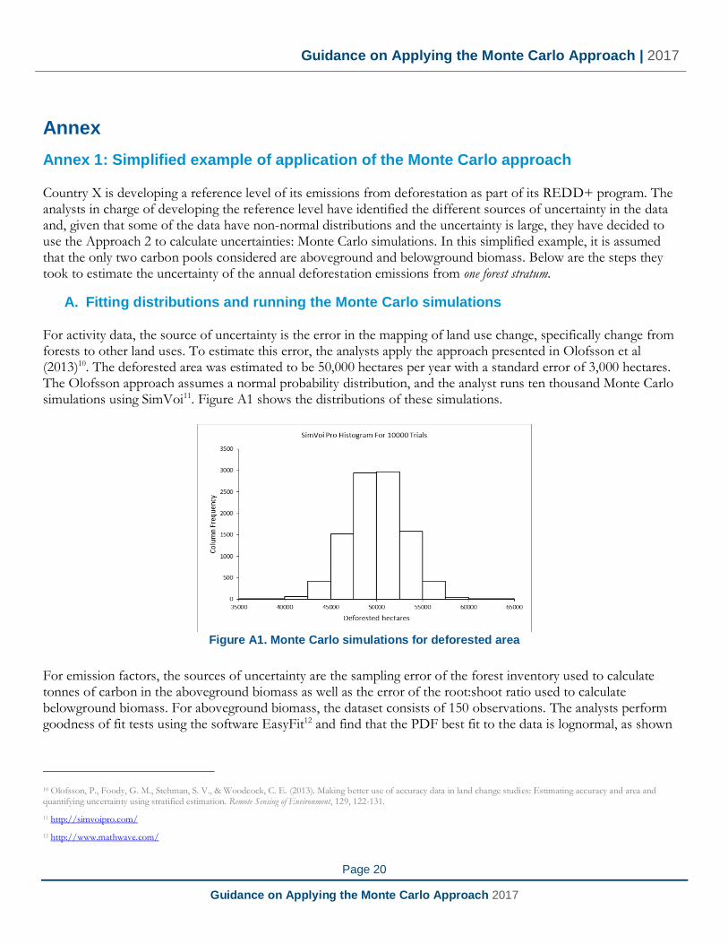
A. Fitting distributions and running the Monte Carlo simulations For activity data, the source of uncertainty is the error in the mapping of land use change, specifically change from forests to other land uses. To estimate this error, the analysts apply the approach presented in Olofsson et al (2013)10. The deforested area was estimated to be 50,000 hectares per year with a standard error of 3,000 hectares. The Olofsson approach assumes a normal probability distribution, and the analyst runs ten thousand Monte Carlo simulations using SimVoi11. Figure A1 shows the distributions of these simulations.

Figure A1. Monte Carlo simulations for deforested area

For emission factors, the sources of uncertainty are the sampling error of the forest inventory used to calculate tonnes of carbon in the aboveground biomass as well as the error of the root:shoot ratio used to calculate belowground biomass. For aboveground biomass, the dataset consists of 150 observations. The analysts perform goodness of fit tests using the software EasyFit12 and find that the PDF best fit to the data is lognormal, as shown

10 Olofsson, P., Foody, G. M., Stehman, S. V., & Woodcock, C. E. (2013). Making better use of accuracy data in land change studies: Estimating accuracy and area and quantifying uncertainty using stratified estimation. Remote Sensing of Environment, 129, 122-131.

11 http://simvoipro.com/

12 http://www.mathwave.com/

http://simvoipro.com/

http://www.mathwave.com/



in Figure A2. Based on the parameters of the fitted distribution that EasyFit provides (=3.8967; =0.15607)13, the analyst can run 10,000 Monte Carlo simulations in SimVoi (Figure A3).

Figure A2. Lognormal distribution fitted to aboveground biomass data

Figure A3. Monte Carlo simulations for tonnes of carbon in aboveground biomass per hectare

The analyst notices, however, some of the simulations produce very high values. In-country experts deem that any values over 90 t C/hectare are unrealistic. As a result, the analyst reruns the simulation, this time truncating the distribution by setting the maximum value at 90, as shown in Figure A4.

13 The analyst must make sure that the parameters provided by the goodness of fit software are the same as the parameters required to run the Monte Carlo simulations. If

not, they need to be converted to the parameters required for the simulations. In this case, and must be converted to mean and standard deviation. The equations to do this can be found at https://www.mathworks.com/help/stats/lognstat.html.

Probability Density Function

Histogram Lognormal

tC/hectare72686460565248444036

f(x)

0.24

0.22

0.2

0.18

0.16

0.14

0.12

0.1

0.08

0.06

0.04

0.02

0

https://www.mathworks.com/help/stats/lognstat.html



Figure A4. Truncated Monte Carlo simulations with a maximum value of 90 tonnes of carbon in aboveground

biomass per hectare

Because there is no country-specific data on belowground biomass, the analysts apply the root:shoot ratio, 0.205, for tropical moist forest (in which category the forest stratum being analyzed falls) that Mokany et al (2006)14 identifies. Because the study provides the standard error, the analyst can run a Monte Carlo simulation based on the assumption that the distribution is normal. The resulting Monte Carlo simulation of the root:shoot ratio is in Figure A5.

Figure A5. Monte Carlo simulations of root:shoot ratio

14 Mokany, K., Raison, R., & Prokushkin, A. S. (2006). Critical analysis of root: shoot ratios in terrestrial biomes. Global Change Biology, 12(1), 84-96.



B. Applying Monte Carlo simulations to equations to calculate uncertainty of total emissions

In order to identify the probability distribution of carbon in belowground biomass, the analyst multiples the simulations of the carbon in aboveground biomass by the simulations of the root:shoot ratio as in the following equation in Figure A6.

Where: BBC = Carbon in belowground biomass, tC ha-1

ABC = Carbon in aboveground biomass, tC ha-1

RSR = root:shoot ratio, dimensionless

Figure A6. Application of Monte Carlo simulations in equation to identify probability distribution of carbon content in belowground biomass



To calculate the total amount of carbon dioxide in the two carbon pools being analyzed (i.e., the emission factor), the simulations of carbon in aboveground and belowground biomass were applied in the equation in Figure A7.

Where: EF = Tonnes of carbon dioxide in above and belowground biomass, t CO2 ha-1

BBC = Carbon in belowground biomass, tC ha-1

ABC = Carbon in aboveground biomass, tC ha-1

44/12 = Conversion factor of carbon to carbon dioxide, dimensionless

Figure A7. Calculating the distribution of emission factor based on the distributions of above and belowground biomass

In order to identify the probability distribution of the total emissions from deforestation for the forest stratum in question (Figure A8), the distributions for the emission factor calculated in Figure A8 are multiplied by the distribution of the Monte Carlo simulations of the activity data (annual deforested area).

Where: Total emission = Tonnes of CO2 emitted, tCO2 year-1

EF = Emission factor; Tonnes of carbon dioxide in above and belowground biomass, t CO2 ha-1

AD = Activity data; area of deforestation, hectares year-1

Figure A8. Calculating the distribution of annual emissions from deforestation in one forest stratum



C. Calculating the confidence interval Once the analysts have the final distributions, they first assess whether or not the distribution is normal. Through a goodness of fit test, they find that the distribution is not normal and, therefore, will apply the bootstrapping method to obtain the confidence interval of the median of the emissions value (which should be the median of the distribution). Figure A9 shows the final distribution of medians as well as the confidence interval calculated through bootstrapping. The final confidence interval width (97,484) is the difference between the 97.5th percentile value (10,940,035) minus the 2.5th percentile value (10,842,551) of the median distribution.

Figure A9. Distribution of medians of final emissions calculated through bootstrapping.

Red lines indicate the 2.5th percentile and 97.5th percentile of the distribution of medians used to identify the final emission distribution confidence interval.



D. Calculating uncertainty To calculate the percent uncertainty, half the confidence interval is divided by the emission estimate (the median of the final emissions distribution) and multiplied by 100.

% 𝑢𝑛𝑐𝑒𝑟𝑡𝑎𝑖𝑛𝑡𝑦 = 0.45% =

12

× (97,484)

10,888,815 × 100

Therefore, the final % uncertainty for emissions from deforestation in one forest stratum is 0.45%. As discussed in Section 5 of the report, this small uncertainty value is the result of the high number of simulations.

guidance on applying the monte carlo approach … · carlo approach to uncertainty analyses in...

Documents