guide to confocal microscopy on the zeiss lsm 510 meta...
TRANSCRIPT

Guide to Confocal Microscopy on the Zeiss LSM 510 META NLO
Criss II Rm 405
Heather Jensen-Smith PhD
402-280-2248

You should go through thesesteps (even if you are using the microscope without the confocal):
1) Turn on the remote control switch
2) Turn on the computer, log in,start the software (“LSM510 META”)
3) Turn the key on the Chameleon to the ON position, if needed (DAPI, 2 photon ex)
SWITCHING ON THE ZEISS LSM 510 CONFOCAL MICROSCOPE

1) HAL – halogen source, 3200K button
2) Field stop, aperture stop, neutral density filters
3) Lens change and filter change buttons on side, behind focus knobs
4) Focus buttons, left side, at the front
5) FL – epi fluorescence source
6) Field stop, aperture stop
7) Epi path block
8) F1, F2 buttons – do not use
Manual operation of the Axioplan 2 microscope

Four Steps to Confocal Image Acquisition:
1. Turn on the laser or lasers
2. Use ‘vis’ mode on microscope to locate area of interest for confocal microscopy switch to LSM mode
3. Select a confocal configuration from the Configuration window
4. Adjust the zoom, orientation, and detector gain using “Fast X-Y”
5. Acquire the image using “Single”
LASER SCANNING CONFOCAL OPERATION

Set slider to “VIS”(in): eyepiece viewing of transmitted light and fluorescence
MICROSCOPE EYEPIECE VIEWING

For laser scanning image acquisition: “LSM” - slider out
LASER SCANNING CONFOCAL OPERATION

1) Double click the LSM 510 icon
2) Select “Scan New Images”
3) Select “Start Expert Mode”
Starting the LSM 510 software
Note 1: Attempting to acquire new images in ‘use existing’ mode will result in a scanned image window with a ‘rainbow pattern,’ exit program then select New Images to correct
Note 2: Rapid microscope initialization (1-2 sec) suggests the confocal was turned on prior to the computer, restart system and/or check microscope power switch to correct

1) Select Acquire LASER CONTROL WINDOW
2) Select laser or lasers
3) Switch required laser/s to Standby (if required) then On
Ar laser tube current should be 5.7 to 5.9. Output [%] should be about 45-50%
List of general fluorochromecolors excited with a given
laser:
Argon = green
HeNe1= red
HeNe2= far reds
Cham= DAPI, 2-photon ex

100
3-5%
CONFIGURATION WINDOW
LASER SELECTION AND ATTENUATION SETTINGS
Use of any laser above these settings may damage or destroy your sample and possibly the lasers! Please attempt to adjust the intensity of your acquired by modifying the sensitivity of the detectors instead.

CONFIGURATION WINDOW
2) Shows the optical configuration (light pathto photodetector used to generate image)
3) Modify by selecting each optical element or load a specific configuration
Your account is pre-loaded with a small number of basic green (Alexa 488,Cy2, FITC), red (Cy3, Rhodamine, Alexa 568) and blue (DAPI) configurations. You may add to and/or modify these to generate a user-specific list of configurations.

CHOOSING THE CONFIGURATION
MULTI TRACK
Use for double or triple labelling
Sequential scanning, line by line or frame by frame
When one track is active, only one detector and one laser is switched on. This dramatically reduces crosstalk.
ADVANTAGES
DISADVANTAGESSlower image acquisition
SINGLE TRACK
Use for single, double labeling (must be spectrally distinct fluorophores)
Simultaneous scanning only
Faster image acquisition
ADVANTAGES
DISADVANTAGESCross talk between channels

CONFIGURATION WINDOW
1) Select single or multi-tract
2) Press the Configuration button
3) Select a stored configuration from this list, press Apply
3) Store any new configuration under a new name if desired

1) Select Config
2) Select Track
SINGLE TRACK – laser/s scan simultaneously
3) Load single track specficconfiguration
(configuration-selected laser/s and attenuation displayed in Ex. Window)
Transmitted lightimages can be generated during Fl imaging. Optical path to ChDdetector located at the back of the microscope (at the base) must be switched to permit TL images to be generated.
CONFIGURATION WINDOW
Note no image is visible through the eyepiece when the light path is open to ChD.
5) Select Apply
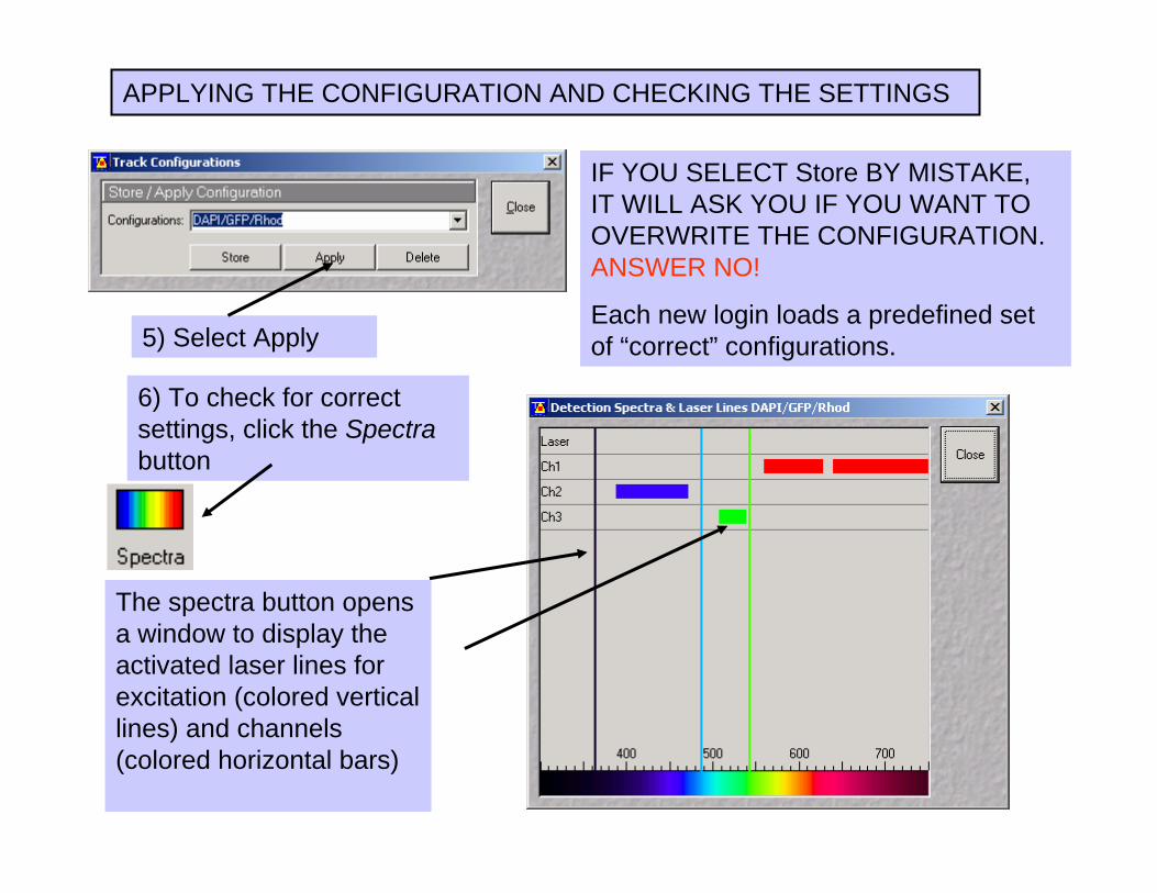
IF YOU SELECT Store BY MISTAKE, IT WILL ASK YOU IF YOU WANT TO OVERWRITE THE CONFIGURATION.ANSWER NO!
Each new login loads a predefined set of “correct” configurations.
APPLYING THE CONFIGURATION AND CHECKING THE SETTINGS
The spectra button opens a window to display the activated laser lines for excitation (colored vertical lines) and channels (colored horizontal bars)
6) To check for correct settings, click the Spectra button

1) Select Scan
SCAN CONTROL WINDOW
2) Select Mode
3) Select the Frame Sizeas predefined number of pixels or enter your own values (e.g. 300 x 600). Use Optimal for calculation of appropriate number of pixels depending on N.A. and λ.
The number of pixels influences the scanning resolution!

Enter the scan speed - a higher speed with averaging gives the best signal to noise ratio. Scan speed 8 usually produces good results. Use 6 or 7 for superior images. The slower the scan, the greater the bleaching.
ENTERING SCAN SPEED

Select the dynamic range - 8 bit will give 256 grey levels, 12 bit will give 4096 levels. Photoshop will import 12 and 16 Bit images.
Publication quality images should be acquired using 12 bit.
SETTING UP THE DYNAMIC RANGE (8/12 Bit per pixel)

The depth of the optical section is dependant on:1) Pinhole diameter(greater pinhole -thicker section)2) Wavelength(longer wavelength -thicker section)3) NA of objective(higher NA -thinner section)
CONFOCAL MICROSCOPE
Features above and below the plane of focus fall outside the pinhole and appear black -producing a true optical section.

CHANNEL SETTINGS - ADJUSTING PINHOLE
1 “Airy units” produces the best signal : noise ratio
Pinhole adjustment changes the Optical slice.
When collecting multi channel images, adjust the pinholes so that each channel has the same Optical Slice. This is important for co-localization studies.
Pinhole size = 1 Airy unit

× NA
10
20
40
60
0.3
0.5
1.3 (oil)
1.4 (oil)
PIXEL SIZE
0.51 µm
0.31 µm
0.12 µm
0.11 µm
MINIMUM PIXEL SIZE DETERMINED BY NYQUIST SAMPLING THEOREM
Adjusting the field size (“XY”) to 56 µm with the 60× lens would produce a pixel size of 0.1 µm
Field size can be adjusted by changing the objective magnification, or by optical zooming. Changing from 40 × to 60 × will reduce the field size, but will also reduce the amount of light available.
Brightness of image = magnification2/NA2
Values are for scan zoom = 1.0

ACQUISITION OF IMAGES
Select “Single”
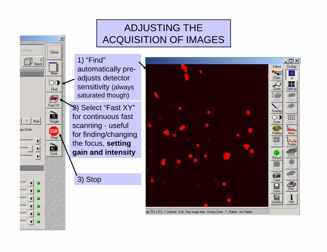
2) Select “Fast XY”for continuous fast scanning - useful for finding/changing the focus, setting gain and intensity
ADJUSTING THE ACQUISITION OF IMAGES
1) “Find”automatically pre-adjusts detector sensitivity (always saturated though)
3) Stop

SELECTING GAIN AND OFFSET - CHOOSING A LOOKUP TABLE
1) Select Palette
2) Select Range Indicator
Red = Saturation (maximum)
Blue = Zero (minimum)

“Detector gain” determines the sensitivity of the detector by setting the maximum limit
“Ampl. Offset” determines the minimum intensity limit
“Ampl. Gain” determines signal amplification
SCAN CONTROL - SETTING GAIN AND OFFSET
Saturation at the maximum →reduce “Gain”
Saturation at the minimum increase “Offset”
Gain set correctly
Offset set correctly
Gain
Offset
Amplifier Gain increases the whole signal, and the offset will need to be decreased.

ADJUSTING GAIN AND OFFSET
1) Increase the Offset until all blue pixels disappear, and then make it slightly positive.
2) Reduce the Gain until the red pixels only just disappear.
Both Gain and Offset saturated

OPTICAL ZOOMING
The level of zoom can be changed either by using the zoom control under “microscope”, or by selecting “Crop” on the image menu
The image can also be rotated by selecting and dragging the bars (Only works with overlapped image)

MULTI TRACK CONFIGURATION
1) Select “Multi Track” for sequential scanning
2) Select “2P-DAPI/Cy2/Cy3”

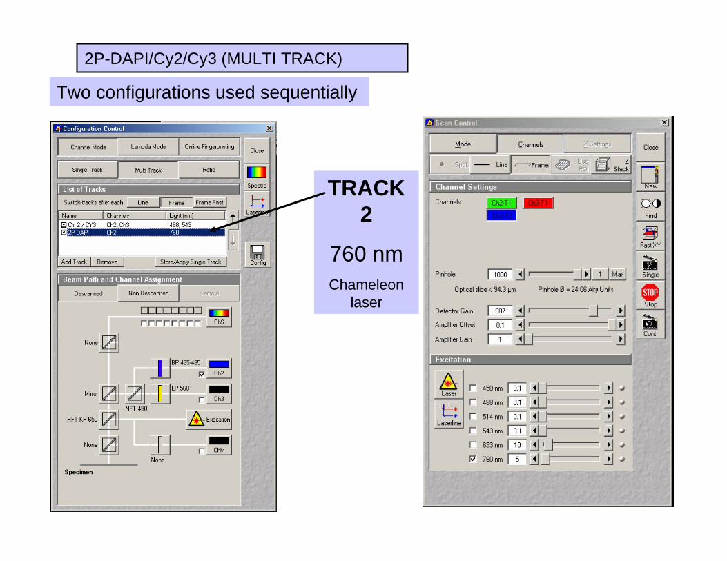
2P-DAPI/Cy2/Cy3 (MULTI TRACK)
Two configurations used sequentially
TRACK 1
488/543 nm,
Ar laser
2P-DAPI/Cy2/Cy3 (MULTI TRACK)
Two configurations used sequentially
TRACK 2
760 nmChameleon
laser

ADJUSTING THE LASER, GAIN AND OFFSET
MULTI-TRACK CONFIGURATION
Each channel is selected independently, and the laser power and other parameters are optimised as described in the previous slides.
For accurate co-localization, adjust the Pinholes so that each channel has the same Optical Slice. 0.8 “Airy units” gives the best signal:noise ratio for normal confocal. Open the pinhole when using the Chameleon – two-photon excitation is inherently confocal and does not require a pinhole.

1) Select Split
2) In Palette, select Range Indicator
3) Select each channel separately under Channels and adjust the Laser, Gain, and Offset as described previously. ***Switching btwn tracks takes time (fast xy is slower), optimize one track at a time (fast xy faster), then view both at same time
Split
SETTING UP GAIN AND OFFSET - MULTI TRACK
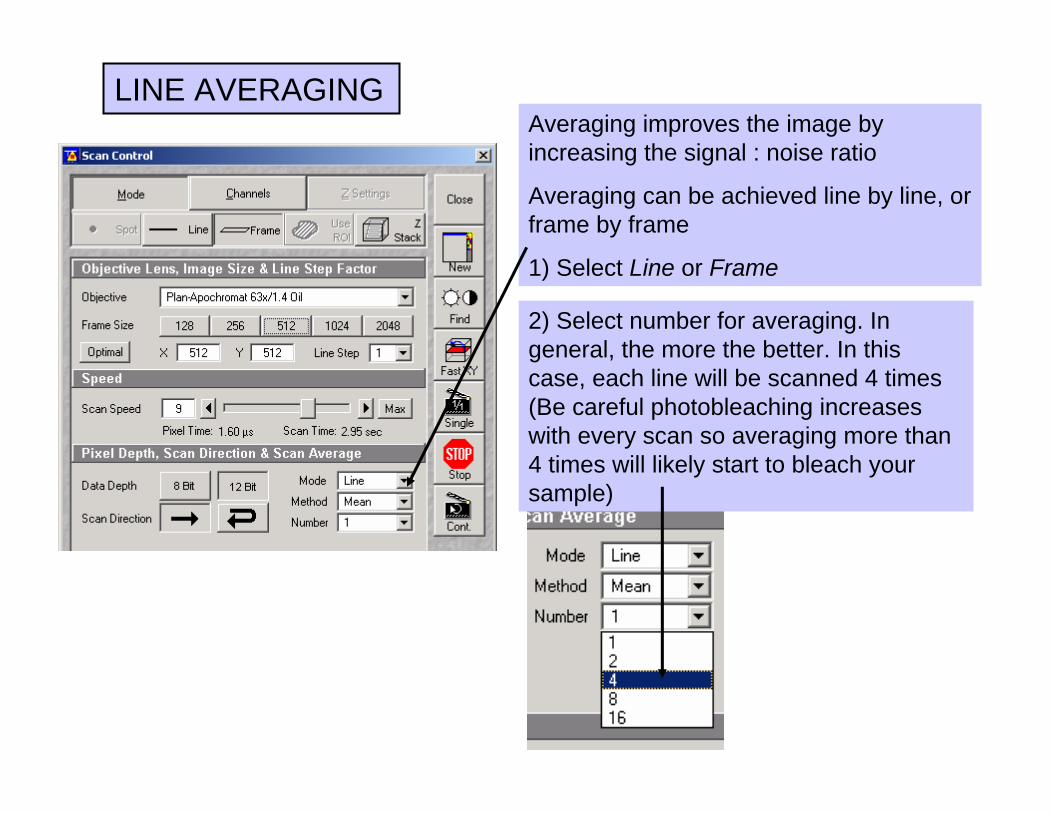
LINE AVERAGING
2) Select number for averaging. In general, the more the better. In this case, each line will be scanned 4 times (Be careful photobleaching increases with every scan so averaging more than 4 times will likely start to bleach your sample)
Averaging improves the image by increasing the signal : noise ratio
Averaging can be achieved line by line, or frame by frame
1) Select Line or Frame

FRAME AVERAGING1) Select “Frame”
2) Select the number for averaging - The more the better (max 16) BUT repeated scans increase bleaching. Continuous averaging is also possible in this mode
Frame averaging helps reduce photobleaching, but does not give quite such a smooth image. There is also a longer delay between each track when using “Multi Track”.
Continuous averaging has a “Finish” button which allows the scan currently in progress to be completed before stopping

COLLECTING AN AVERAGED IMAGE
1) Return to Mode, and under Scan Average select the number for the average.
Under “Channels” select single”. An averaged image will be collected.
Range indicator switched off

SCANNING A Z SERIES USING “MARK FIRST/LAST”
1) Select “Z Stack”
2) Start scanning using “Fast XY” or “XY Cont”
3) Keep your eye on the image and move the focus to the beginning of the Z series - select “Mark First”
4) Move the focus back in the opposite direction to the end of the Z series, and select “Mark Last”
5) X:Y:Z sets the Z-interval so that the voxel has identical dimensions in X, Y, Z.
6) with Auto Z Corr., Detector Gain, AOTF, Ampl. Offset and Ampl. Gain can be varied between two (A, B) freely selectable slices of a stack
NOTEFocusing can be achieved manually (preferred), or using “Stage” on the LSM menu
Focus
Increment
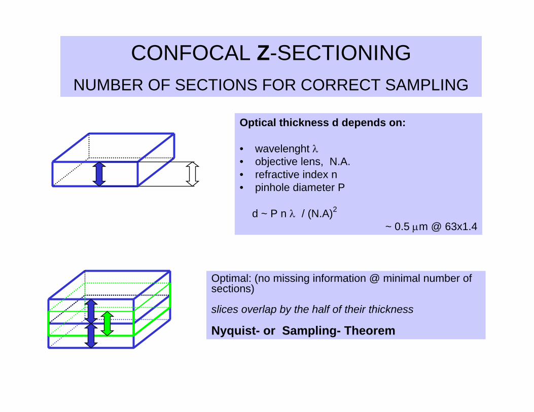
CONFOCAL Z-SECTIONINGNUMBER OF SECTIONS FOR CORRECT SAMPLING
Optical thickness d depends on:
• wavelenght λ• objective lens, N.A.• refractive index n• pinhole diameter P
d ~ P n λ / (N.A)2
~ 0.5 µm @ 63x1.4
Optimal: (no missing information @ minimal number of sections)
slices overlap by the half of their thickness
Nyquist- or Sampling- Theorem

Z STACK - NUMBER OF SLICES AND INCREMENT
1) Select Z slice - the window Optical Slice will appear
2) Select Optimal interval the computer will calculate the optimum number of sections
3) Select “Start”
For more or less sections -adjust Num Slices

Z - SERIES USING “Z SECTIONING”
1) Select Z Stack
2) Select Z Sectioning
3) Select Line Sel
4) Select the large arrow button and position the XZ cut line

1) Decide whether to Keep Interval or Keep Slices
2) Select “Range” and position bars to decide where the Z - series begins and ends
3) Select “Start”
Z SECTIONING - SETTING RANGE
Vertical section of sample
Set limits for Z-Series

VIEWING A Z - SERIES
1) Select “xy”
2) Select “Slice”
3) Use scroll bar to view individual sections

VIEWING A Z - SERIES USING GALLERY
1) Select Gallery
2) Select Data
for scale
Use Subset to extract sections

VIEWING Z- SERIES USING ORTHOGONAL SECTIONS
1) select Ortho 2) Select mouse
( Select)
3) Using the mouse, position the cut lines.
To save orthogonal sections, select Exportand save as contents of image window.

SELECTING AND SAVING A REGION OF INTEREST
1) Select Overlay and define shape for ROI
2) Select “Extract region”
3) Save data

USING “EDIT ROI” FOR FASTER IMAGE ACQUISITION AND DATA SAVING
1) Select “EditROI” from the LSM menu bar
2) Select “Fit Frame Size to bounding Rectangle”3) Choose ROI shape
4) position and size with mouse
5) Scan
To remove ROI select blue bin
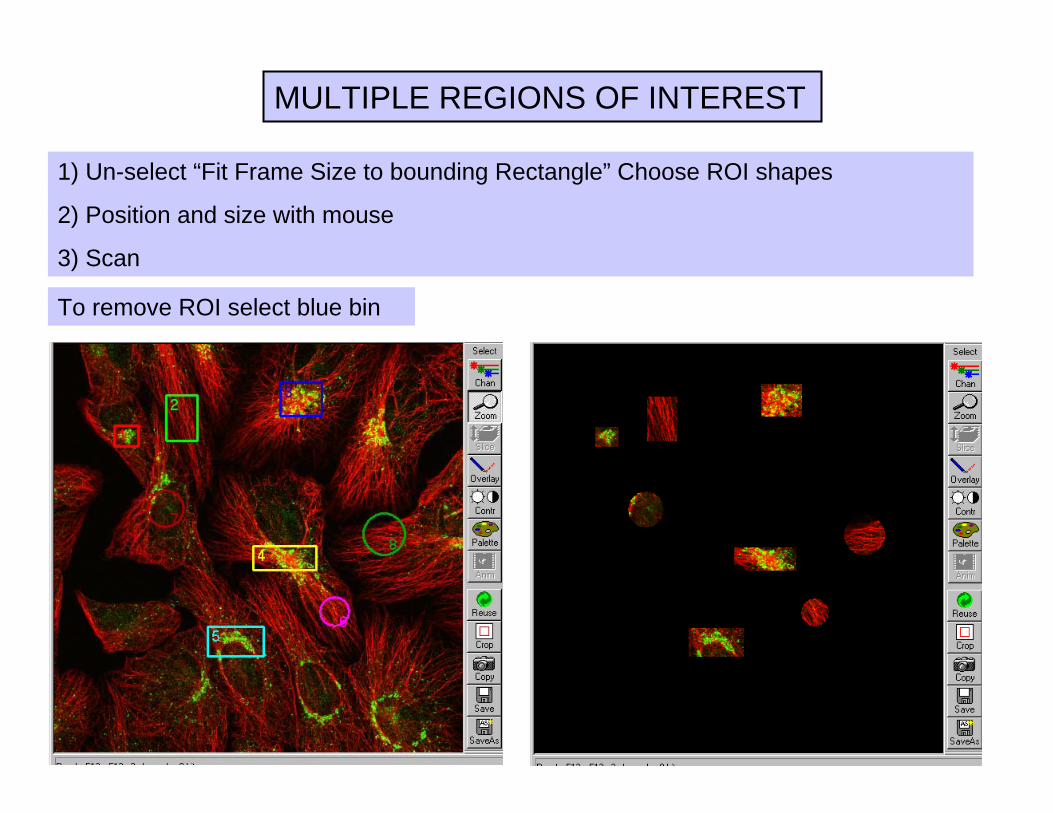
MULTIPLE REGIONS OF INTEREST
1) Un-select “Fit Frame Size to bounding Rectangle” Choose ROI shapes
2) Position and size with mouse
3) Scan
To remove ROI select blue bin

TIME SERIES
1) Set up scanning parameters (Z-Series)
2) Select “Time series” from the LSM menu
3) Select “min,”“sec” or “ms”
4) Enter the number of cycles
5) Select “Start T”

VIEWING A TIME SERIES
Z Sections for any time
Time points for any Z Section
Both Z sections and time series

TIME SERIES - PHYSIOLOGY EXPERIMENTS
1) If required, use multiple regions of interest
2) Set up time series as before
3) Instead of using “TimeSeries”, select “MeanROI” to start scanning
View and save data by selecting

IMAGING A LARGE AREA USING TILING
1) Select “Stage”on LSM menu
2) Enter the “Tile Numbers”
3) Select “Start”
3 3

TILED IMAGEAny position can then be marked and a single image acquired by selecting “Move to” and then single

SAVING DATA - USING DATABASE
1) Select “Save or “Save as” on image window or LSM menu bar
2) Select an existing or generate (and name) a new database to save your images to. Please save to the ‘Big Disk’
3) Then generate a file name for your image and notes if required
3) Select “OK”
4) Save subsequent images to this DB or a generate a new one
Remember images do not exist without a database so be sure to transfer an entire database when saving files to DVD’s for future use. You must open the entire .mbddatabase to select individual images for export, ect.

1) Select “New” database
2) Select drive Big Disk H: from pull down menu
3) Save to your folder on the H drive
Creating a database for acquired images

SAVING INDIVIDUAL IMAGE FILES - USING “EXPORT”
1) Select “File”from LSM menu
2) Select “Export”
3) Select “Image type”
4) Select “Single image with raw data,” “Series with raw data,” or “Contents of image window”
5) Select “Save as type”
“Tif - Tagged Image File” is OK for 8 bit - use “Tiff -16 bit”for 12 bit acquired images. Most other software will not recognize 12 bit.

SHUT DOWN PROCEDURE (cont’d)1. Acquire - Laser - Switch off lasers
•Allow the Ar & HeNe lasers time to cool (light turns off)
•Turn the key on the Chameleon to Standby•log out •shut down the computer IF it’s the weekend or after 5pm (i.e., you don’t anticipate anyone else using the scope in the next hour)

SHUT DOWN PROCEDURE (cont’d)
2. File - Exit LSM 510 program.3. Go to Windows START, shut down computer operating system.4. Turn off the remote control switch.

• Please sign a terms of use agreement before using the microscope– Include contact info for the person responsible for billing,
your fund/org numbers (CU only) and a billing address– Non-Cu researchers will receive monthly invoices (PO # are
accepted with prior approval), CU researchers will be automatically billed, statements are sent out at the beginning of the month
• Please site the CUIBIF in all your publications:“This research was conducted at the Integrative Biological Imaging Facility at Creighton University, Omaha, NE. This facility, supported by the C.U. Medical School, was constructed with support from C06 Grant RR17417-01 from the
NCRR, NIH.”
Questions?Contact : Heather [email protected]
CUIBIF Billing Address/ Remit payment to:Mary Anne KeefeDepartment of Biomedical Sciences, Criss II Rm 3132500 California PlazaOmaha, NE 68178402-280-2015