guide to intelligent data analysis - william & marykemper/cs626/slides/gida4.pdf · data...
TRANSCRIPT
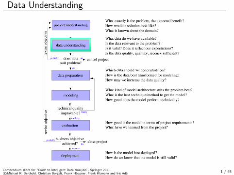
Data Understanding
Compendium slides for “Guide to Intelligent Data Analysis”, Springer 2011.c©Michael R. Berthold, Christian Borgelt, Frank Hoppner, Frank Klawonn and Iris Ada 1 / 45
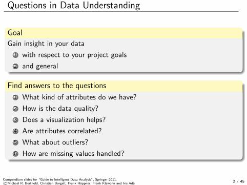
Questions in Data Understanding
Goal
Gain insight in your data
1 with respect to your project goals
2 and general
Find answers to the questions
1 What kind of attributes do we have?
2 How is the data quality?
3 Does a visualization helps?
4 Are attributes correlated?
5 What about outliers?
6 How are missing values handled?
Compendium slides for “Guide to Intelligent Data Analysis”, Springer 2011.c©Michael R. Berthold, Christian Borgelt, Frank Hoppner, Frank Klawonn and Iris Ada 2 / 45

Attribute understanding
We (often) assume that the data set is provided in the form of a simpletable.
attribute1 . . . attributem
record1...
recordn
The rows of the table are called instances, records or data objects.
The columns of the table are called attributes, features or variables.
Compendium slides for “Guide to Intelligent Data Analysis”, Springer 2011.c©Michael R. Berthold, Christian Borgelt, Frank Hoppner, Frank Klawonn and Iris Ada 3 / 45
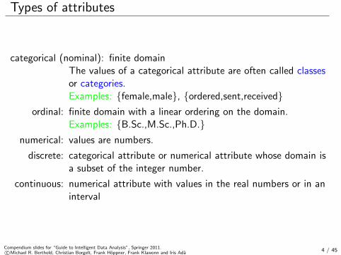
Types of attributes
categorical (nominal): finite domainThe values of a categorical attribute are often called classesor categories.Examples: {female,male}, {ordered,sent,received}
ordinal: finite domain with a linear ordering on the domain.Examples: {B.Sc.,M.Sc.,Ph.D.}
numerical: values are numbers.
discrete: categorical attribute or numerical attribute whose domain isa subset of the integer number.
continuous: numerical attribute with values in the real numbers or in aninterval
Compendium slides for “Guide to Intelligent Data Analysis”, Springer 2011.c©Michael R. Berthold, Christian Borgelt, Frank Hoppner, Frank Klawonn and Iris Ada 4 / 45
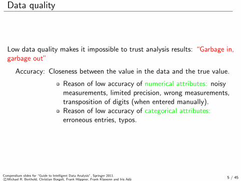
Data quality
Low data quality makes it impossible to trust analysis results: “Garbage in,garbage out”
Accuracy: Closeness between the value in the data and the true value.
Reason of low accuracy of numerical attributes: noisymeasurements, limited precision, wrong measurements,transposition of digits (when entered manually).Reason of low accuracy of categorical attributes:erroneous entries, typos.
Compendium slides for “Guide to Intelligent Data Analysis”, Springer 2011.c©Michael R. Berthold, Christian Borgelt, Frank Hoppner, Frank Klawonn and Iris Ada 5 / 45
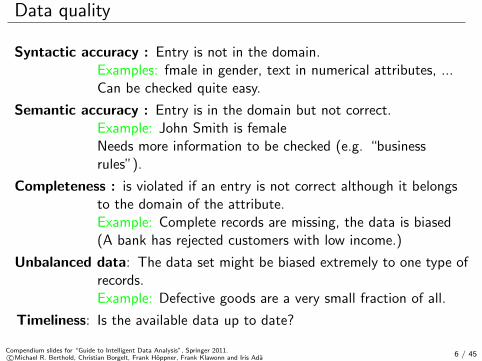
Data quality
Syntactic accuracy : Entry is not in the domain.Examples: fmale in gender, text in numerical attributes, ...Can be checked quite easy.
Semantic accuracy : Entry is in the domain but not correct.Example: John Smith is femaleNeeds more information to be checked (e.g. “businessrules”).
Completeness : is violated if an entry is not correct although it belongsto the domain of the attribute.Example: Complete records are missing, the data is biased(A bank has rejected customers with low income.)
Unbalanced data: The data set might be biased extremely to one type ofrecords.Example: Defective goods are a very small fraction of all.
Timeliness: Is the available data up to date?
Compendium slides for “Guide to Intelligent Data Analysis”, Springer 2011.c©Michael R. Berthold, Christian Borgelt, Frank Hoppner, Frank Klawonn and Iris Ada 6 / 45

Data visualisation
Tukey: There is no excuse for failing to plot and look.
Compendium slides for “Guide to Intelligent Data Analysis”, Springer 2011.c©Michael R. Berthold, Christian Borgelt, Frank Hoppner, Frank Klawonn and Iris Ada 7 / 45

Hidden missing values
0 5 10 15 200
1
2
3
4
5
time
win
d sp
eed
The zero values might come from a broken or blocked sensor and might beconsider as missing values.
Compendium slides for “Guide to Intelligent Data Analysis”, Springer 2011.c©Michael R. Berthold, Christian Borgelt, Frank Hoppner, Frank Klawonn and Iris Ada 8 / 45
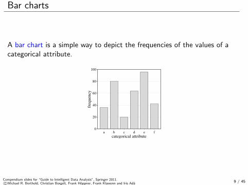
Bar charts
A bar chart is a simple way to depict the frequencies of the values of acategorical attribute.
a b c d e f0
20
40
60
80
100
categorical attribute
freq
uenc
y
Compendium slides for “Guide to Intelligent Data Analysis”, Springer 2011.c©Michael R. Berthold, Christian Borgelt, Frank Hoppner, Frank Klawonn and Iris Ada 9 / 45

Histograms
A histogram shows the frequency distribution for a numerical attribute.The range of the numerical attribute is discretized into a fixed number ofintervals (called bins), usually of equal length. For each interval the(absolute) frequency of values falling into it is indicated by the height of abar.
–3 –2 –1 0 1 2 3 4 5 6 70
25
50
75
100
125
150
175
numerical attribute
freq
uenc
y
Compendium slides for “Guide to Intelligent Data Analysis”, Springer 2011.c©Michael R. Berthold, Christian Borgelt, Frank Hoppner, Frank Klawonn and Iris Ada 10 / 45
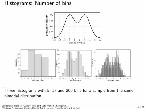
Histograms: Number of bins
–3 –2 –1 0 1 2 3 4 5 60
0.05
0.1
0.15
0.2
attribute valuepr
obab
ility
den
sity
–3 –2 –1 0 1 2 3 4 5 6 70
50
100
150
200
250
300
350
attribute value
freq
uenc
y
–3 –2 –1 0 1 2 3 4 5 6 70
20
40
60
80
100
120
attribute value
freq
uenc
y
–3 –2 –1 0 1 2 3 4 5 6 70
5
10
15
attribute value
freq
uenc
yThree histograms with 5, 17 and 200 bins for a sample from the samebimodal distribution.
Compendium slides for “Guide to Intelligent Data Analysis”, Springer 2011.c©Michael R. Berthold, Christian Borgelt, Frank Hoppner, Frank Klawonn and Iris Ada 11 / 45
Histograms: Number of bins
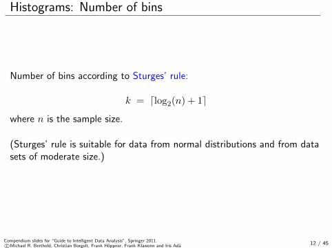
Number of bins according to Sturges’ rule:
k = dlog2(n) + 1e
where n is the sample size.
(Sturges’ rule is suitable for data from normal distributions and from datasets of moderate size.)
Compendium slides for “Guide to Intelligent Data Analysis”, Springer 2011.c©Michael R. Berthold, Christian Borgelt, Frank Hoppner, Frank Klawonn and Iris Ada 12 / 45
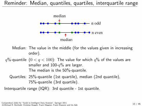
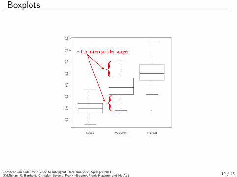
Reminder: Median, quantiles, quartiles, interquartile range
Median: The value in the middle (for the values given in increasingorder).
q%-quantile (0 < q < 100): The value for which q% of the values aresmaller and 100-q% are larger.The median is the 50%-quantile.
Quartiles: 25%-quantile (1st quartile), median (2nd quantile),75%-quantile (3rd quartile).
Interquartile range (IQR): 3rd quantile - 1st quantile.
Compendium slides for “Guide to Intelligent Data Analysis”, Springer 2011.c©Michael R. Berthold, Christian Borgelt, Frank Hoppner, Frank Klawonn and Iris Ada 13 / 45
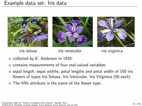
Example data set: Iris data
iris setosa iris versicolor iris virginica
collected by E. Anderson in 1935
contains measurements of four real-valued variables:
sepal length, sepal widths, petal lengths and petal width of 150 irisflowers of types Iris Setosa, Iris Versicolor, Iris Virginica (50 each)
The fifth attribute is the name of the flower type.
Compendium slides for “Guide to Intelligent Data Analysis”, Springer 2011.c©Michael R. Berthold, Christian Borgelt, Frank Hoppner, Frank Klawonn and Iris Ada 14 / 45
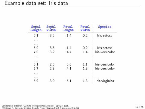
Example data set: Iris data
Sepal Sepal Petal Petal SpeciesLength Width Length Width
5.1 3.5 1.4 0.2 Iris-setosa......5.0 3.3 1.4 0.2 Iris-setosa7.0 3.2 4.7 1.4 Iris-versicolor......5.1 2.5 3.0 1.1 Iris-versicolor5.7 2.8 4.1 1.3 Iris-versicolor......5.9 3.0 5.1 1.8 Iris-virginica
Compendium slides for “Guide to Intelligent Data Analysis”, Springer 2011.c©Michael R. Berthold, Christian Borgelt, Frank Hoppner, Frank Klawonn and Iris Ada 15 / 45

Boxplots
Compendium slides for “Guide to Intelligent Data Analysis”, Springer 2011.c©Michael R. Berthold, Christian Borgelt, Frank Hoppner, Frank Klawonn and Iris Ada 16 / 45

Boxplots
Compendium slides for “Guide to Intelligent Data Analysis”, Springer 2011.c©Michael R. Berthold, Christian Borgelt, Frank Hoppner, Frank Klawonn and Iris Ada 17 / 45
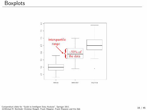
Boxplots
Compendium slides for “Guide to Intelligent Data Analysis”, Springer 2011.c©Michael R. Berthold, Christian Borgelt, Frank Hoppner, Frank Klawonn and Iris Ada 18 / 45
Boxplots
Compendium slides for “Guide to Intelligent Data Analysis”, Springer 2011.c©Michael R. Berthold, Christian Borgelt, Frank Hoppner, Frank Klawonn and Iris Ada 19 / 45
Boxplots
Compendium slides for “Guide to Intelligent Data Analysis”, Springer 2011.c©Michael R. Berthold, Christian Borgelt, Frank Hoppner, Frank Klawonn and Iris Ada 20 / 45
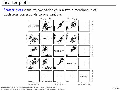
Scatter plots
Scatter plots visualize two variables in a two-dimensional plot.Each axes corresponds to one variable.
Compendium slides for “Guide to Intelligent Data Analysis”, Springer 2011.c©Michael R. Berthold, Christian Borgelt, Frank Hoppner, Frank Klawonn and Iris Ada 21 / 45

Scatter plots
5 6 7 8
2
2.5
3
3.5
4
4.5
sepal length / cm
sepa
l wid
th /
cm
Iris setosaIris versicolorIris virginica
Scatter plots can be enriched with additional information: Colour ordifferent symbols to incorporate a third attribute in the scatter plot.
Compendium slides for “Guide to Intelligent Data Analysis”, Springer 2011.c©Michael R. Berthold, Christian Borgelt, Frank Hoppner, Frank Klawonn and Iris Ada 22 / 45

Scatter plots
1 2 3 4 5 6 70
0.5
1
1.5
2
2.5
petal length / cm
peta
l wid
th /
cm
Iris setosaIris versicolorIris virginica
The two attributes petal length and width provide a better separation ofthe classes Iris versicolor and Iris virginica than the sepal length and width.
Compendium slides for “Guide to Intelligent Data Analysis”, Springer 2011.c©Michael R. Berthold, Christian Borgelt, Frank Hoppner, Frank Klawonn and Iris Ada 23 / 45

Scatter plots
1 2 3 4 5 6 70
0.5
1
1.5
2
2.5
petal length / cm
peta
l wid
th /
cm
Iris setosaIris versicolorIris virginica
Data objects with the same values cannot be distinguished in a scatterplot. To avoid this effect, jitter is used, i.e. before plotting the points,small random values are added to the coordinates. Jitter is essential forcategorical attributes.
Compendium slides for “Guide to Intelligent Data Analysis”, Springer 2011.c©Michael R. Berthold, Christian Borgelt, Frank Hoppner, Frank Klawonn and Iris Ada 24 / 45
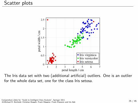
Scatter plots
1 2 3 4 5 6 70
0.5
1
1.5
2
2.5
petal length / cm
peta
l wid
th /
cm
Iris setosaIris versicolorIris virginica
The Iris data set with two (additional artificial) outliers. One is an outlierfor the whole data set, one for the class Iris setosa.
Compendium slides for “Guide to Intelligent Data Analysis”, Springer 2011.c©Michael R. Berthold, Christian Borgelt, Frank Hoppner, Frank Klawonn and Iris Ada 25 / 45
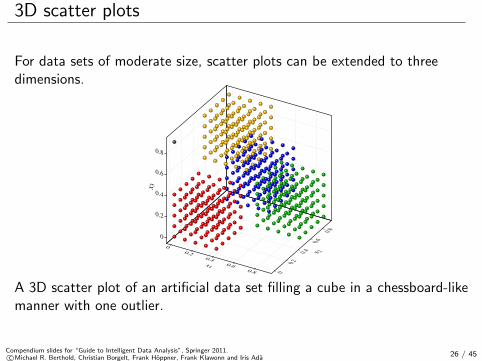
3D scatter plots
For data sets of moderate size, scatter plots can be extended to threedimensions.
00.2
0.40.6
0.8 00.2
0.40.6
0.80
0.2
0.4
0.6
0.8
x1
x 2
x 3
A 3D scatter plot of an artificial data set filling a cube in a chessboard-likemanner with one outlier.
Compendium slides for “Guide to Intelligent Data Analysis”, Springer 2011.c©Michael R. Berthold, Christian Borgelt, Frank Hoppner, Frank Klawonn and Iris Ada 26 / 45
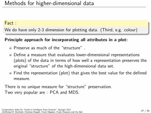
Methods for higher-dimensional data
Fact :
We do have only 2-3 dimension for plotting data. (Third, e.g. colour)
Principle approach for incorporating all attributes in a plot:
Preserve as much of the “structure” .
Define a measure that evaluates lower-dimensional representations(plots) of the data in terms of how well a representation preserves theoriginal “structure” of the high-dimensional data set.
Find the representation (plot) that gives the best value for the definedmeasure.
There is no unique measure for “structure” preservation.Two very popular are : PCA and MDS.
Compendium slides for “Guide to Intelligent Data Analysis”, Springer 2011.c©Michael R. Berthold, Christian Borgelt, Frank Hoppner, Frank Klawonn and Iris Ada 27 / 45
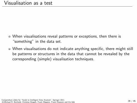
Visualisation as a test
When visualisations reveal patterns or exceptions, then there is“something” in the data set.
When visualisations do not indicate anything specific, there might stillbe patterns or structures in the data that cannot be revealed by thecorresponding (simple) visualisation techniques.
Compendium slides for “Guide to Intelligent Data Analysis”, Springer 2011.c©Michael R. Berthold, Christian Borgelt, Frank Hoppner, Frank Klawonn and Iris Ada 28 / 45

Parallel coordinates
Parallel coordinates draw the coordinate axes parallel to each other, sothat there is no limitation for the the number of axes to be displayed.
For a data object, a polyline is drawn connecting the values of the dataobject for the attributes on the corresponding axes.
Compendium slides for “Guide to Intelligent Data Analysis”, Springer 2011.c©Michael R. Berthold, Christian Borgelt, Frank Hoppner, Frank Klawonn and Iris Ada 29 / 45

Parallel coordinates: Iris data
sepallength
sepalwidth
petallength
petalwidth species
Iris setosaIris versicolorIris virginica
sepallength
sepalwidth
petallength
petalwidth
sepallength
sepalwidth
petallength
petalwidth
sepallength
sepalwidth
petallength
petalwidth
Compendium slides for “Guide to Intelligent Data Analysis”, Springer 2011.c©Michael R. Berthold, Christian Borgelt, Frank Hoppner, Frank Klawonn and Iris Ada 30 / 45

Parallel coordinates: “Cube data”
x1 x2 x3
Compendium slides for “Guide to Intelligent Data Analysis”, Springer 2011.c©Michael R. Berthold, Christian Borgelt, Frank Hoppner, Frank Klawonn and Iris Ada 31 / 45

Radar plots
Radar plots are based on a similar idea as parallel coordinates with thedifference that the coordinate axes are drawn as parallel lines, but in astar-like fashion intersecting in one point.
sepal length
sepal widthpetal length
petal width
Iris setosaIris versicolorIris virginica
Radar plot for the Iris data set
Compendium slides for “Guide to Intelligent Data Analysis”, Springer 2011.c©Michael R. Berthold, Christian Borgelt, Frank Hoppner, Frank Klawonn and Iris Ada 32 / 45
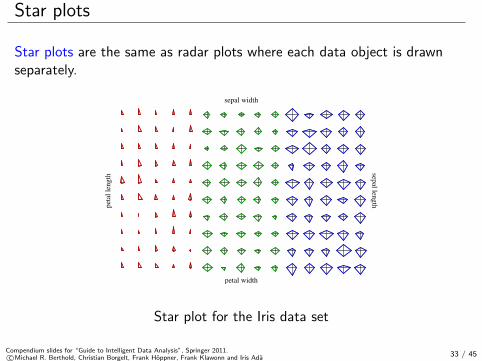
Star plots
Star plots are the same as radar plots where each data object is drawnseparately.
sepal lengthsepal width
peta
l len
gth
petal width
Star plot for the Iris data set
Compendium slides for “Guide to Intelligent Data Analysis”, Springer 2011.c©Michael R. Berthold, Christian Borgelt, Frank Hoppner, Frank Klawonn and Iris Ada 33 / 45

Correlation Analysis
How can the similiar behaviour of two attributes be proved?
Pearson’s correlation coefficient
Spearman’s rank correlation coefficient (Spearman’s rho)
more in the book ...
Compendium slides for “Guide to Intelligent Data Analysis”, Springer 2011.c©Michael R. Berthold, Christian Borgelt, Frank Hoppner, Frank Klawonn and Iris Ada 34 / 45
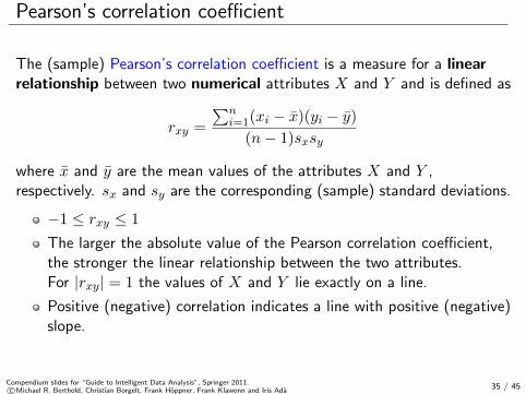
Pearson’s correlation coefficient
The (sample) Pearson’s correlation coefficient is a measure for a linearrelationship between two numerical attributes X and Y and is defined as
rxy =
∑ni=1(xi − x)(yi − y)
(n− 1)sxsy
where x and y are the mean values of the attributes X and Y ,respectively. sx and sy are the corresponding (sample) standard deviations.
−1 ≤ rxy ≤ 1
The larger the absolute value of the Pearson correlation coefficient,the stronger the linear relationship between the two attributes.For |rxy| = 1 the values of X and Y lie exactly on a line.
Positive (negative) correlation indicates a line with positive (negative)slope.
Compendium slides for “Guide to Intelligent Data Analysis”, Springer 2011.c©Michael R. Berthold, Christian Borgelt, Frank Hoppner, Frank Klawonn and Iris Ada 35 / 45
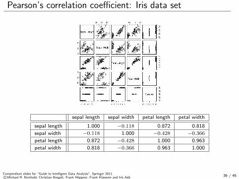
Pearson’s correlation coefficient: Iris data set
sepal length sepal width petal length petal width
sepal length 1.000 −0.118 0.872 0.818
sepal width −0.118 1.000 −0.428 −0.366
petal length 0.872 −0.428 1.000 0.963
petal width 0.818 −0.366 0.963 1.000
Compendium slides for “Guide to Intelligent Data Analysis”, Springer 2011.c©Michael R. Berthold, Christian Borgelt, Frank Hoppner, Frank Klawonn and Iris Ada 36 / 45
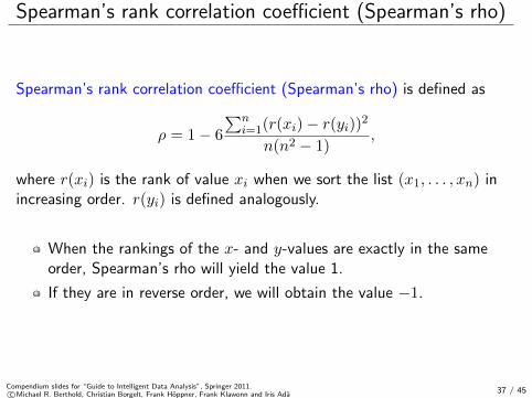
Spearman’s rank correlation coefficient (Spearman’s rho)
Spearman’s rank correlation coefficient (Spearman’s rho) is defined as
ρ = 1− 6
∑ni=1(r(xi)− r(yi))2
n(n2 − 1),
where r(xi) is the rank of value xi when we sort the list (x1, . . . , xn) inincreasing order. r(yi) is defined analogously.
When the rankings of the x- and y-values are exactly in the sameorder, Spearman’s rho will yield the value 1.
If they are in reverse order, we will obtain the value −1.
Compendium slides for “Guide to Intelligent Data Analysis”, Springer 2011.c©Michael R. Berthold, Christian Borgelt, Frank Hoppner, Frank Klawonn and Iris Ada 37 / 45

Spearman’s rho: Iris data set
sepal length sepal width petal length petal width
sepal length 1.000 −0.167 0.882 0.834
sepal width −0.167 1.000 −0.289 −0.289
petal length 0.882 −0.289 1.000 0.938
petal width 0.834 −0.289 0.938 1.000
Compendium slides for “Guide to Intelligent Data Analysis”, Springer 2011.c©Michael R. Berthold, Christian Borgelt, Frank Hoppner, Frank Klawonn and Iris Ada 38 / 45
Outlier detection
An outlier is a value or data object that is far away or very different fromall or most of the other data.
Causes for outliers:
Data quality problems (erroneous data coming from wrongmeasurements or typing mistakes)
Exceptional or unusual situations/data objects.
Outliers coming from erroneous data should be excluded from theanalysis.
Even if the outliers are correct (exceptional data), it is sometimeuseful to exclude them from the analysis.For example, a single extremely large outlier can lead to completelymisleading values for the mean value.
Compendium slides for “Guide to Intelligent Data Analysis”, Springer 2011.c©Michael R. Berthold, Christian Borgelt, Frank Hoppner, Frank Klawonn and Iris Ada 39 / 45

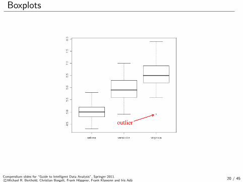
Outlier detection: Single attributes
Categorical attributes: An outlier is a value that occurs with a frequencyextremely lower than the frequency of all other values.Numerical attributes:
Outliers in boxplots.
Statistical tests, for example Grubb’s test: ... (see the exercise)
Compendium slides for “Guide to Intelligent Data Analysis”, Springer 2011.c©Michael R. Berthold, Christian Borgelt, Frank Hoppner, Frank Klawonn and Iris Ada 40 / 45
Outlier detection for multidimensional data
Scatter plots for (visually detecting) outliers w.r.t. two attributes.
PCA or MDS plots for (visually detecting) outliers.
Cluster analysis techniques: Outliers are those points which cannot beassigned to any cluster.
Compendium slides for “Guide to Intelligent Data Analysis”, Springer 2011.c©Michael R. Berthold, Christian Borgelt, Frank Hoppner, Frank Klawonn and Iris Ada 41 / 45

Missing values
For some instances values of single attributes might be missing.
Causes for missing values:
broken sensors
refusal to answer a question
irrelevant attribute for the corresponding object(pregnant (yes/no) for men)
Missing value might not necessarily be indicated as missing (instead: zeroor default values).
Compendium slides for “Guide to Intelligent Data Analysis”, Springer 2011.c©Michael R. Berthold, Christian Borgelt, Frank Hoppner, Frank Klawonn and Iris Ada 42 / 45

Types of missing values
Consider the attribute Xobs. A missing value is denoted by ?. X is thetrue value, i.e. we have Xobs = X, if Xobs 6=? Let Y be all otherattributes apart from X.
Missing completely at random (MCAR): The probability that avalue for X is missing does neither depend on the true value of X noron other variables.
P (Xobs =?) = P (Xobs =? | X,Y )
Missing at random (MAR): The probability that a value for X ismissing does not depend on the true value of X.
P (Xobs =? | Y ) = P (Xobs =? | X,Y )
Nonignorable: The probability that a value for X is missing dependson the true value of X.
Compendium slides for “Guide to Intelligent Data Analysis”, Springer 2011.c©Michael R. Berthold, Christian Borgelt, Frank Hoppner, Frank Klawonn and Iris Ada 43 / 45

A checklist for data understanding
Determine the quality of the data. (e.g. syntactic accuracy)
Find outliers. (e.g. using visualization techniques)
Detect and examine missing values. Possible hidden by default values.
Discover new or confirm expected dependencies or correlationsbetween attributes.
Check specific application dependent assumptions (e.g. the attributefollows a normal distribution)
Compare statistics with the expected behavior.
Compendium slides for “Guide to Intelligent Data Analysis”, Springer 2011.c©Michael R. Berthold, Christian Borgelt, Frank Hoppner, Frank Klawonn and Iris Ada 44 / 45

A checklist for data understanding: Must Do
Check the distributions for each attribute(unexpected properties like outliers, correct domains, correct medians)
Check correlations or dependencies between pairs of attributes
Compendium slides for “Guide to Intelligent Data Analysis”, Springer 2011.c©Michael R. Berthold, Christian Borgelt, Frank Hoppner, Frank Klawonn and Iris Ada 45 / 45