gujarat technological university ahmedabad february …
TRANSCRIPT

Implementation and Computation of Performance
Excellence in Connecting Rod Manufacturing Industries
A Thesis submitted to Gujarat Technological University
For the Award of
Doctor of Philosophy
in
Mechanical Engineering
by
Sunilkumar Sureshchandra Sonigra
Enrollment No. : 119997119012
Under supervision of
Dr. M. N. Qureshi
GUJARAT TECHNOLOGICAL UNIVERSITY
AHMEDABAD
February 2017

ii

iii
Implementation and Computation of Performance
Excellence in Connecting Rod Manufacturing Industries
A Thesis submitted to Gujarat Technological University
For the Award of
Doctor of Philosophy
in
Mechanical Engineering
By
Sunilkumar Sureshchandra Sonigra
Enrollment No. : 119997119012
Under supervision of
Dr. M. N. Qureshi
GUJARAT TECHNOLOGICAL UNIVERSITY
AHMEDABAD
February 2017

iv
© Sunilkumar Sureshchandra Sonigra

v
DECLARATION
I declare that the thesis entitled “Implementation and Computation of Performance
Excellence in Connecting Rod Manufacturing Industries” submitted by me for the degree
of Doctor of Philosophy, is the record of research work carried out by me during the period
from October 2011 to October 2016 under the supervision of Dr. M. N. Qureshi, Associate
Professor - Mechanical Engineering Department, Faculty of Technology and Engineering, The
M. S. University of Baroda, Vadodara and Dr. Kash A. Barker, Professor, Oklahoma
University, Oklahoma, USA, and this has not formed the basis for the award of any degree,
diploma, associate ship and fellowship, titles in this or any other University or other institution
of higher learning.
I further declare that the material obtained from other sources has been duly acknowledged in
the thesis. I shall be solely responsible for any plagiarism or other irregularities, if noticed in
the thesis.
Signature of the Research Scholar: _____________________ Date:02-02-2017
Name of Research Scholar: Sunilkumar Sureshchandra Sonigra
Place: Ahmedabad.

vi
CERTIFICATE
I certify that the work incorporated in the thesis titled as Implementation and
Computation of Performance Excellence in Connecting Rod Manufacturing Industries
submitted by Mr. Sunilkumar Sureshchandra Sonigra was carried out by the candidate
under my supervision/guidance. To the best of my knowledge: (i) the candidate has not
submitted the same research work to any other institution for any degree/diploma,
Associateship, Fellowship or other similar titles (ii) the thesis submitted is a record of original
research work done by the Research Scholar during the period of study under my supervision,
and (iii) the thesis represents independent research work on the part of the Research Scholar.
Signature of Supervisor: Date: 02-02-2017
Name of Supervisor: Dr. M. N. Qureshi
Place: Ahmedabad.

vii
Originality Report Certificate
It is certified that PhD Thesis titled Implementation and Computation of Performance
Excellence in Connecting Rod Manufacturing Industries submitted by Mr. Sunilkumar
Sureshchandra Sonigra has been examined by me. I undertake the following:
a. Thesis has significant new work / knowledge as compared already published or are
under consideration to be published elsewhere. No sentence, equation, diagram, table,
paragraph or section has been copied verbatim from previous work unless it is placed
under quotation marks and duly referenced.
b. The work presented is original and own work of the author (i.e. there is no plagiarism).
No ideas, processes, results or words of others have been presented as Author own
work.
c. There is no fabrication of data or results which have been compiled / analyzed.
d. There is no falsification by manipulating research materials, equipment or processes,
or changing or omitting data or results such that the research is not accurately
represented in the research record.
e. The thesis has been checked using https://turnitin.com (copy of originality report
attached) and found within limits as per GTU Plagiarism Policy and instructions issued
from time to time (i.e. permitted similarity index <=25%).
Signature of Research Scholar: …………….. Date: 02-02-2017
Name of Research Scholar: Sunilkumar Sureshchandra Sonigra
Place: Ahmedabad
Signature of Supervisor: …………….. Date: 02-02-2017
Name of Supervisor: Dr. M. N. Qureshi
Place: Ahmedabad

viii
Copy of Originality Report
FILE TIME SUBMITTED SUBMISSION ID
PH.D_THESIS.PDF (2.23M) 17-OCT-2016 09:03AM 721859566
WORD COUNT CHARACTER COUNT
31294 148822
Checked using https://turnitin.com

ix
Ph. D. THESIS Non-Exclusive License to
GUJARAT TECHNOLOGICAL UNIVERSITY
In consideration of being a Ph. D. Research Scholar at GTU and in the interests of the
facilitation of research at GTU and elsewhere, I, Sunilkumar Sureshchandra Sonigra having
Enrollment No. 119997119012 hereby grant a non-exclusive, royalty free and perpetual
license to GTU on the following terms:
a) GTU is permitted to archive, reproduce and distribute my thesis, in whole or in part,
and/or my abstract, in whole or in part ( referred to collectively as the “Work”)
anywhere in the world, for non-commercial purposes, in all forms of media;
b) GTU is permitted to authorize, sub-lease, sub-contract or procure any of the acts
mentioned in paragraph (a);
c) GTU is authorized to submit the Work at any National / International Library, under
the authority of their “Thesis Non-Exclusive License”;
d) The Universal Copyright Notice (©) shall appear on all copies made under the
authority of this license;
e) I undertake to submit my thesis, through my University, to any Library and Archives.
Any abstract submitted with the thesis will be considered to form part of the thesis.
f) I represent that my thesis is my original work, does not infringe any rights of others,
including privacy rights, and that I have the right to make the grant conferred by this
non-exclusive license.
g) If third party copyrighted material was included in my thesis for which, under the terms of
the Copyright Act, written permission from the copyright owners is required, I have

x
obtained such permission from the copyright owners to do the acts mentioned in paragraph (a)
above for the full term of copyright protection.
h) I retain copyright ownership and moral rights in my thesis, and may deal with the
copyright in my thesis, in any way consistent with rights granted by me to my University
in this non-exclusive license.
i) I further promise to inform any person to whom I may hereafter assign or license my
copyright in my thesis of the rights granted by me to my University in this non- exclusive
license.
j) I am aware of and agree to accept the conditions and regulations of PhD including all
policy matters related to authorship and plagiarism.
Signature of Research Scholar:………………... Date: 02-02-2017
Name of Research Scholar: Sunilkumar Sureshchandra Sonigra
Place: Ahmedabad
Signature of Supervisor: ………………... Date: 02-02-2017
Name of Supervisor: Dr. M. N. Qureshi
Place: Ahmedabad
Seal:

xi
Annexure - VII
Thesis Approval Form
The viva-voce of the Ph.D. Thesis submitted by Shri Sunilkumar Sureshchandra Sonigra
(Enrollment No. 119997119012) entitled Implementation and Computation of
Performance Excellence in Connecting Rod Manufacturing Industries was conducted on
…………………….., (day and date) at Gujarat Technological University.
(Please tick any one of the following option)
We recommend that he be awarded the Ph.D. degree.
We recommend that the viva-voce be re-conducted after incorporating the following
suggestions.
(briefly specify the modifications suggested by the panel)
The performance of the candidate was unsatisfactory. We recommend that he should
not be awarded the Ph.D. degree.
(The panel must give justifications for rejecting the research work)
--------------------------------------------------
Name and Signature of Supervisor with Seal
---------------------------------------------------
External Examiner -1 Name and Signature
---------------------------------------------------
External Examiner -2 Name and Signature
--------------------------------------------------
External Examiner -3 Name and Signature

xii
ABSTRACT
The present work explains the solutions of ongoing industrial problems in details related to
connecting rod manufacturing operations. The solutions of each problem may not be
generalized. Every existing problem is having Tailor-Made Solution (TMS). The probably
diversified options for the solutions are identified and discussed with statistical measures. The
necessary remedial measures are executed for shop floor activities for the individual case. The
impacts of implemented actions for each case are discussed in details. The proposed solutions
are justified by the feedback of implemented action.
The existing problems are identified from Customer Complaints Redressal Form (CCRF),
Rework analysis, Rejection report, In-process Inspection Report (IIR), Final Inspection Report
(FIR), Doc Inspection Report (DIR), Patrol Inspection Report (PIR), Process Capability Study
Report (PCSR) and on-going shop floor production report. Five problems are identified related
to connecting rod manufacturing and solutions to be implemented for individual cases.
The solutions for on-going shop floor production issues are derived with various problem-
solving techniques. The brainstorming session, Cause and Effect Diagram (CED) (Fish Bone
Diagram), Pareto Analysis, Failure Mode and Effects Analysis (FMEA), Kaizen, etc.; are used
for Tailor-Made Solution (TMS) of individual cases. The solutions proposed are implemented
to solve the respective production issues.
Various Quality Improvement tools are employed in various industries by many experts in one
or another form in manufacturing industries. The gap is identified that there is no generalized
methodology to solve the on-going problem. There is a need to generate the general steps to
identify the non-conformance potential and to implement the necessary actions. There are
numerous ways to identify improvement potential and implement the same with the higher
degree of impact.
The thesis addresses five major questions in connecting rod manufacturing industries (1)
Higher rejection in bush boring operation (2) dent marks in the small end (3) End float
variation (4) Bend and Twist (5) Big End bore diameter variation of connecting rod.

xiii
Acknowledgement
I am very much thankful to respected Sirs, Dr. M. N. Qureshi, Dr. G. D. Acharya and Dr. M.
G. Bhatt for their continuous encouragement, guidance and tremendous support. I am also
thankful to respected Sir, Dr. Kash A. Barker, for invaluable guidance with International
Exposure for my work. The studies described in this thesis were performed at Rajkot base
Manufacturing Industries. While conducting this research project I received support from
many people in one way or another, without whose support, this thesis would not have been
completed in its present form. It is my pleasure to take this opportunity to thank all of you. I
would like to apologize to those I do not mention by name here; however, I highly valued your
kind support.
I am also oblige to Dr. Anil K. kulkarni, Dr. J. A. Vadher, Dr. H. K. Raval, Dr. K. P. Desai,
Dr. A. V. Gohil, Dr. Mitesh Popat, Dr. Rajbir Singh, Dr. P. K. Brahmbhatt, Mr. Parag Solanki
and Mr. Dilip Patel for their untiring effort and guidance for the present work. I am equally
obliging to the staff members of my institution, Government Polytechnic, Rajkot for their
positive approach and continuous support. Further, I would like to express my great thanks to
Comissionerate of Technical Education, Gujarat state, for allowing me to do the research
work.
Last but not least, my parents and my family members Neha, Devam, Diva… … … I have no
word to say…
And above of all, to the supreme power who is the originator of all these occurrences, we call
as GOD for my entire life.
S. S. Sonigra
Date : 02.02.2017

xiv
Table of Contents
Page No.
Declaration V
Project Approval page vi
Originality Report Certificate vii
Ph. D. Thesis Non-Exclusive License to GTU ix
Thesis Approval Form xi
Abstract xii
Acknowledgement xiii
Table of Contents xiv
List of Abbreviation ix
List of Tables xix
List of Figures xxiii
List of Appendices xxiv
References xxv
1. INTRODUCTION 1
1.1 Motivation
1.2 Background
1.3 Boundary conditions
1.4 The Constraints
1.5 Original contribution by the thesis
1.6 Research objectives
1.7 Structure of the Thesis
2. LITERATURE SURVEY AND PROBLEM IDENTIFICATION 12
2.1 Review of research work
2.2 Research gap
2.3 Research Methodology
2.4 Definition of problem

xv
3. COMPUTATION OF OVERALL EQUIPMENT EFFECTIVENESS FOR
CONNECTING ROD MANUFACTURING OPERATIONS 19
3.1 Introduction
3.2 Review of other research
3.3 Objectives of OEE
3.4 Implementation
3.5 OEE factors and Computation sheet
3.6 Analysis
3.7 Results and discussion
3.8 Limitations for using OEE system
3.9 Summary
4. IMPLEMENTATION OF BUSH BORING CHAMFER TO AVOID MANUAL
DE-BURRING IN CONNECTING ROD: A KAIZEN APPROACH 32
4.1 Introduction
4.2 Literature Review
4.3 Research Methodology
4.4 Problem Statement
4.5 Kaizen Sheet
4.6 Feasibility of Proposed solution
4.7 Concluding remarks
5. CONTROL VARIATION IN END FLOAT PARAMETER WITH THE
APPLICATION OF SIX SIGMA TOOLS 38
5.1 Introduction
5.2 Literature Review
5.3 Six Sigma frame work
5.4 Problem Statement
5.4.1 Meaning of End Float
5.4.2 Computation sheet of End Float
5.5 DMAIC

xvi
5.5.1 Define
5.5.2 Measure
5.5.3 Analyze
5.5.4 Improve
5.5.5 Control
5.6 Return on Quality
5.7 Conclusion
6. QUALITY ASSURANCE IN AXIAL ALIGNMENT (BEND AND TWIST) OF
CONNECTING ROD 53
6.1 Introduction
6.2 Theoretical background
6.3 Bend and Twist of connecting rod and its measurement methods
6.3.1 Method 1 : Measurement with two pins
6.3.2 Method 2 : Measurement with V block
6.3.3 Method 3 : Measurement with Co-ordinate Measuring Machine
6.3.4 Method 4 : Measurement with Special Purpose Gauge
6.4 Interpretation of readings and proposed action plan
6.5 Process Capability Report
6.6 Discussion of implemented action
6.7 Points to be considered while conducting SPC analysis
6.8 Conclusion
7. EXAMINING THE INFLUENCE OF TEMPERATURE VARIATION ON THE
DIMENSIONAL VARIABILITY OF CONNECTING ROD DURING
MANUFACTURING 67
7.1 Introduction
7.2 Literature Review
7.3 Problem Statement
7.4 Readings at various temperatures
7.5 Proposed solutions

xvii
7.6 Conclusion
8. SOLVING THE PROBLEM OF BIG END BORE DIAMETER VARIATION
75
8.1 Introduction
8.2 Literature Review
8.3 The Problem Statement
8.4 Measurement report
8.5 Analysis of brain storming report
8.6 Fishbone diagram
8.7 Discussion of proposed action plan
8.7.1 P-PAP Type 1
8.7.2 P-PAP Type 2
8.7.3 Gauge R and R study (MSA)
8.7.4 STAR technique
8.7.5 Patrol Inspection and Dock Inspection
8.7.6 First Article Inspection
8.8 FMEA : Failure Mode and Effects Analysis
8.9 Data collection
8.10 Analysis phase
8.10.1 First iteration
8.10.2 Second iteration
8.10.3 Third iteration
8.10.4 Fourth iteration
8.11 Process study capability report compilation
8.12 Implemented action plan
8.13 Conclusion
9. COMPUTATION OF PERFORMANCE EXCELLENCE 91
9.1 Performance Excellence parameters
9.2 Graphical representation of performance

xviii
9.3 Objectives Achieved
9.4 Conclusion
9.5 Future Scope
10. REFERENCES

xix
List of Abbreviations
APQP : Advanced Production Quality Planning
CA : Corrective Action
CBA : Cost Benefit Analysis
CCRF : Customer Complaint Redressal Form
CD : Center Distance
CED : Cause and Effect Diagram
CTQ : Critical to Quality
DIR : Dock Inspection Report
DPMO : Defects Per Million Opportunity
FIR : Final Inspection Report
FMEA : Failure Mode and Effect Analysis
FPA : First Piece Approval
IIR : In-process Inspection Report
ISO : International Standardizations for Organization
LCL : Lower Control Limit
LSL : Lower Specification Limit
LTL : Lower Tolerance Limit
MSA : Measuring System Analysis
OEE : Overall Equipment Effectiveness
PA : Preventive Action
PCI : Process Capability Index
PCSR : Process Capability Study Report
PDI : Pre Dispatch Inspection Report

xx
PIR : Patrol Inspection Report
P-PAP : Production Part Approval Process
PPM : Parts Per Million
QA : Quality Assurance
QC : Quality Control
QS : Quality Standards
SPC : Statistical Process Control
SPG : Special Purpose Gauge
SPM : Special Purpose Machine
SQC : Statistical Quality Control
STAR : Situation, Task, Action and Result
TMS : Tailor Made Solution
TPM : Total Productive Maintenance
TQC : Total Quality Control
TQM : Total Quality Management
UCL : Upper Control Limit
USL : Upper Specification Limit
UTL : Upper Tolerance Limit
WCM : World Class Manufacturing
ZD : Zero Defect

xxi
List of Figures
No. Figure Page
1.1 Boundary Condition 5
2.1 Rejection parameters in connecting rod 16
3.1 Fishbone diagram showing rejection potentials 28
3.2 Variation in Center Distance before implementation (More variation) 29
3.3 Variation in Center Distance After implementation (Less variation) 29
3.4 Rework % (monthly) 29
3.5 Rejection % (monthly) 29
3.6 Customer Complaints (monthly) 29
4.1 Manual De burring operation (Before implementation) 35
4.2 Small End Bush Chamfering with Pillar Drill (After Implementation) 35
4.3 Pillar Drilling machine 36
4.4 Fixture for implemented action 36
5.1 End float of connecting rod 43
5.2 Six Sigma Process 44
5.3 Pareto Chart 45
5.4 Cause and Effect Diagram for End Float 48
5.5 Taper ness of Big End Face of Rod and Surface of Fixture 49
5.6 Fixture alteration proposed for solution 50
6.1 Connecting Rod assembly 54
6.2 Buckling of Connecting Rod about Y-axis 55
6.3 Buckling of Connecting Rod about X-axis 55
6.4 I-section of Connecting Rod 56
6.5 Measurement of bend and twist of connecting rod 59
7.1 Temperature variation effect on Big End Bore Diameter 70
7.2 Temperature variation effect on Center Distance 70
7.3 (a) Mechanical Gauge (b) Pneumatic Gauge readings with master. 71
7.4 Big End Bore Diameter correction factor 72
7.5 Center Distance correction factor 73

xxii
8.1 Big end bore diameter measurement 76
8.2 Fish Bone Diagram for Bore Diameter Variation 79
8.3 Process FMEA Sheet 83
8.4 First Iteration 85
8.5 Second Iteration 86
8.6 Third Iteration 87
8.7 Fourth Iteration 88
9.1 Rework % year wise 105
9.2 Rejection % year wise 105
9.3 Production per year 105

xxiii
List of Tables
Page
1.1 Connecting Rod Manufacturing Operations 07
2.1 Rejection Parameters during connecting rod manufacturing 15
2.2 Details of Major rejection parameters 18
3.1 Computation Sheet of OEE for each operation 26
5.1 Computation Sheet of End Float 42
6.1 Process Capability Study Report for Bend 62
6.2 Process Capability Study Report for Twist 63
7.1 Readings at various temperature 69
7.2 Correction Factor at various temperature 72
8.1 Readings of Big End Bore Diameter 77
8.2 Brain-storming Computation sheet 79
8.3 Process Capability Report First Iteration 85
8.4 Process Capability Study Report Second Iteration 86
8.5 Process Capability Study Report Third Iteration 87
8.6 Process Capability Report Fourth Iteration 88
8.7 Compiled Process Capability Study Report 89
9.1 Big End Bore Diameter 93
9.2 Small End Boring (Parent bore-without bush) 94
9.3 Bolt Hole Drilling 95
9.4 Center Distance 96
9.5 Bend (Axial Mis-alignment) 97
9.6 Small End Diameter (After Bush Boring) 98
9.7 Twist (Axial Mis-alignment) 99
9.8 Rework Quantity year wise 100
9.9 Rejection Quantity year wise 103
9.10 Parameter wise Total Rework 106
9.11 Parameter wise Total Rejection 107

xxiv
List of Appendices
Appendix A: Published Articles

Motivation
1
CHAPTER – 1
Introduction
The present work deals with the solutions for an immediate problem facing an industrial
organization. Hence, it comes under the category of Applied Research. The principal aim of
applied research is to discover a solution for some practical problems [1]. The problems arise
in the industry day by day with numerous of varieties and diversities. These problems are
solved with some concealed approaches to retain secrecy policy.
1.1 Motivation
It is needed to materialize the hidden approaches conducted in industries for the solution of
existing problems. There is a need to generalize the structure that can be useful for solving any
industrial challenge. The generalization and implementation of various Tailor-Made Solutions
are discussed in details with the appropriate outcome in the present work.
The visit and interaction with various industries were conducted at the initial stage. The
reviews of concerned persons lead to identifying the need for some firm groundwork. It is
concluded to participate with them for in-depth study with technical aspects of day to day
activities. There are so many hidden constraints while working on the shop floor of any
organization. All those aspects are discussed in details in the present work.
Initially, the approach of management towards the modification found to be challenging. It is
obvious that employment of modification becomes challenging at any workstation. The
commitment of top management towards continuous improvement imparted lots of
encouragement to perform in-depth work and achieve the assigned duty. The management

Chapter-1 Introduction
2
permitted working with certain conditions as per company policy. The initial success in a
minor work becomes the great motivation for further work.
1.2 Background
The significance of modification for the best option has been long recognized as a vital to both
competition and survival in the present competitive business world. There are numerous ways
to identify improvement potential and implement the same with the highest degree of impact.
Various tools used to express the enhancement potential in industries are ISO:9000
(International Standardization for Organization), QS:9000 (Quality Standard), Quality Circles,
Zero Defect (ZD), Six Sigma, TQM (Total Quality Management), WCM (World Class
Manufacturing), Kaizen (workplace improvement), Lean manufacturing, TPM (Total
Productive Maintenance), TQC (Total Quality Control) and much more.
There has been significant research carried out to improve shop floor production activity with
due impact. Various aspects are implemented in many organizations to express the
improvement. After implementation of these aspects, there are equal chances of success and
failure. The success of any action purely depends on the elementary aspects employed for
implementation. There should be micro analysis at every step of actions for real impact of
success. The area of present work is based on these aspects. The research gap is identified in
this field to express the impact of the implemented action.
The present work explains the solutions of ongoing industrial problems in details related to
connecting rod manufacturing operations. The solutions of each problem may not be
generalized. Every existing problem is having Tailor-Made Solution (TMS). The probably
diversified options for the solutions are identified and discussed with statistical measures. The
necessary remedial measures are implemented for shop floor activities for an individual case.
The impacts of implemented actions for each case are discussed in details. The proposed
corrective action plan is justified by feedback of implemented action.
The existing problems are identified from study of Customer Complaints Redressal Form
(CE), Rework analysis, Rejection report, In-process Inspection Report (IIR), Final Inspection
Report (FIR), Doc Inspection Report (DIR), Patrol Inspection Report (PIR), Process

Boundary Condition
3
Capability Study Report (PCSR), Pre-Dispatch Inspection (PDI) Report and on-going shop
floor production report. Five problems are identified related to connecting rod manufacturing
and solutions to be implemented for individual cases.
The solutions for problems raised during shop floor production are derived with various
problem-solving techniques. The brainstorming session, Cause and Effect Diagram (CED)
(Fishbone Diagram), Pareto Analysis, Failure Mode and Effects Analysis (FMEA), Kaizen,
etc, are used for Tailor-Made Solution (TMS) of individual cases. The solutions proposed are
implemented to solve the respective production issues.
Various Quality Improvement tools are employed in various industries by many experts in one
or another form in manufacturing industries. The gap is identified that there is no generalized
methodology to solve the on-going problem. There is a need to generate the general steps to
identify the non-conformance potential and to implement the necessary actions.
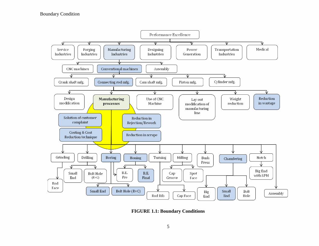
1.3 Boundary Condition
The boundary conditions represented in Fig. 1.1 represent the justification for selection of
present work. Performance Excellence can be employed in Service industries, forging
industries, manufacturing industries, designing industries, power generation and transportation
industries and in the medical field. The present work is concentrated in manufacturing
industries. After visiting many industries, it’s found that there is scope for improvement in
manufacturing industries using the conventional machine where more burning issues are found
as far as quality and quantity is concerned.
The internal combustion engine parts manufacturer produces many parts of an engine. Main
parts are a crankshaft, connecting rod, camshaft, piston, cylinder, piston ring, oil ring,
gudgeon pin, etc. The scope is found in manufacturing processes of the connecting rod. The
connecting rod of Internal Combustion Engine is one of the most critical components of the
mechanism.
The function of the connecting rod is to transmit the reciprocating motion of a piston into
rotary motion of the crankshaft. The piston is a reciprocating element; crankshaft is a rotating

Chapter-1 Introduction
4
element while the connecting rod is an oscillating element of the mechanism. The forging of
connecting rod is followed by various machining operations. There are many hidden
improvement potentials in connecting rod manufacturing operations, which are solved day by
day as and when arisen.
Performance excellence in connecting rod manufacturing includes uses of CNC machines;
layout modification of manufacturing line, weight reduction, reduction in wastage,
modification in manufacturing processes, reduction in rejection or rework, reduction in the
customer complaint, etc.
The present work is performed at manufacturing industries based in Gujarat, dealing with the
manufacturing of various auto parts of Internal Combustion Engine. The connecting rod faces
few problems like dent marks in the small end after the manual deburring operation, End
Float, more rework and rejection at customer end due to the variation in big end bore
diameter. All the problems are identified and solved with Tailor-Made Solution (TMS) up to
the considerable extent.
Boundary Condition
5
FIGURE 1.1: Boundary Conditions

Chapter-1 Introduction
6
1.4 The Constraints
The implementation of the methodology for a particular solution results in many hurdles for
industries as it requires changes in on-going shop floor activities. Change is always rejected at
the first time for any normal working environment. It is a great task to convince the people for
alteration in their regular work. It’s needed to justify the proposed alteration with many
aspects including quality, quantity, cost, comfort and many other aspects. All the hurdles are
solved using practical and tailor-made approach for a particular action.
There are few constraints as listed below to be considered while implementing the corrective
action of any problem.
- It is not allowed to alter any design parameter of the product as it is the customer
requirement. The product is manufactured as per customer drawing, hence it can’t be
altered.
- The manufacturing line of the product should not be disturbed, which may result in the
reduction in production quantity.
- To implement any alteration, the prior permission should be taken from top
management with proper justification.
- The data and documentation of the organization should not be shared anywhere
without prior permission of management.
- The confidentiality of the project work to be maintained as per the management policy.
Considering the above constraints in mind, the present work is selected as represented in
boundary conditions Fig. 1.1.
There are Twenty Three machining operations to be carried out on a forged connecting rod.
Table 1.1 shows the sequence of manufacturing operations needed for the final product.
Advanced Product Quality Planning (APQP) for the product was conducted earlier by the
company people before starting the production. APQP is a structured method of defining the
steps necessary to ensure that a product satisfies the customer requirements.

Original Contribution by the thesis
7
TABLE 1.1 : Connecting Rod Manufacturing Operations
Sr. Name of Operation
Sr. Name of Operation
10 Final Cap Facing 130 Bolt Hole Final Drilling
20 Rod Face Grinding 140 Bolt Hole Cotation
30 Small End Drilling 150 Deburring, Washing and Assembly
40 Small End Final Boring 160 Big End Final Boring
50 Small End Chamfer 170 Big End Chamfer
60 Round Rib Turning 180 Opening and Notch Milling
70 Rough Joint Face (Rod & Cap) 190 Deburring, Washing, Cleaning and Assembly
80 Final Parting Face (Rod & Cap) 200 Big End Rough Honing
90 Cap Groove Milling 210 Big End Final Honing
100 Final Spot Face (Rod & Cap) 220 Small End Bush Pressing and Oil Hole Drilling
110 Big End Locater Boring 230 Small End Bush Boring
120 Bolt Hole Pre Drilling Final Inspection
1.5 Contribution by literature
The present work is applied research and not fundamental research. It deals with the solution
of the ongoing problem facing an industry. Fundamental research is concerned with
generalizations and formulation of a theory. The central aim of applied research is to discover
a solution for some practical problem [1].
The cases are discussed and implemented with various aspects of due impact. The impact of
implemented action is measured with various parameters. The parameters are rejection
quantity per month, rework quantity per month, Customer satisfaction (customer complaint
per month).
The solution of case studies represented in present work can be generalized with the following
steps. Any shop floor issue related to connecting rod manufacturing can be solved by using
these steps.
1. P-PAP (Type 1): The first step is to prepare a report of Production Part Approval
Process Type 1. Check alignment (straightness) of the fixture with respect to the
reference plane. Any deviation more than allowable limit leads to inaccurate output.
Take appropriate action to eliminate such deviation.

Chapter-1 Introduction
8
2. P-PAP (Type 2): Prepare a report of Production Part Approval Process Type-2.
Measure the spindle axial alignment with respect to the reference surface. Do
necessary alteration if the deviation is more than allowable range.
3. Gauge R & R Study (MSA): Check the measuring instruments and gauge with a
master calibration unit. (Measurement System Analysis, Gauge Repeatability and
Reproducibility Study)
4. Interact with Operator and Inspector for the fitness to do work with STAR technique.
(Situation, Task, Action and Result) [2] [3]
5. Reports: Check the Patrol Inspection and Dock Inspection Reports.
6. Prepare First Article Inspection Report (FAIR) and may alter the frequency.
7. FMEA : Do Failure Mode and Effects Analysis for the case if needed. Prepare the
chart of readings. Try to find out the trend of Non-conformance, e.g. Tool change
frequency, coolant temperature, operator, inspector, instrument, etc. (To find the
impact of the respective factor responsible for Non-conformance)
1.6 Research Objectives
The objectives for present work are
• To identify the improvement potential in manufacturing processes of the connecting
rod.
• To maintain customer satisfaction with the implementation of Quality Control tools
(Kaizen and Zero Defect).
• To solve shop floor issues related to Connecting Rod manufacturing operations.
• To implement Performance Excellence in Connecting Rod Manufacturing Industries.
1.7 Structure of the Thesis

Structure of the Thesis
9
Chapter 1 gives a brief description of the research work. It includes background and
motivation for present work. The boundary conditions are represented along with the pre-
defined constraints for present work. It also covers the research objectives and original
contribution by the thesis.
Chapter 2 covers the Literature review related to present work and research gap identified
after rigorous literature survey. The Research methodology employed is also discussed in
details in this chapter.
Chapter 3 presents the method for computation of Overall Equipment Effectiveness (OEE) in
connecting rod manufacturing processes. The OEE sheet enables companies to attain a rapid
assessment of their operations performance. It highlights the gray area of the shop floor. The
OEE sheet discussed is a dominant tool to evaluate the current state and to plan the future state
of enterprise operations. This sheet is employed in a connecting rod manufacturing industries
to provide decision-makers with adequate input to identify improvement objectives and review
the ongoing operations strategy. The use of OEE sheet is demonstrated and some perceptions
are extracted and mentioned regarding the sheet’s applicability for different types of
manufacturing operations.
Chapter 4 The purpose of this chapter is to identify and outline the application of Kaizen
approach on the shop floor of manufacturer of the connecting rod. After a bush boring
operation, in Small End of connecting rod, pillar drill is used to eliminate dent marks and
burrs, as a replacement for manual de-burring operation. It reduces manual work with better
concentricity of small end and improves the quality of product up to a considerable extent.
Assembly of gudgeon pin in the small end of connecting rod becomes easier as compared to
the previous method due to chamfered end. The efforts made by teamwork to employ kaizen
concept is documented and discussed in details.
Chapter 5 covers the discussion and solution of a technical problem identified from
customer complaint redressal form . The study examines one of the shop floors long-lasting
quality issues to maintain the End Float in a connecting rod during the manufacturing process.
This study leverages various Six Sigma tools such as “Fishbone diagram, histograms, control
charts and brainstorming” to provide the platform for essential actions. The analysis resulted

Chapter-1 Introduction
10
in a number of findings and recommendations. The corrective actions for the problem are
discussed and implemented which improves the customer satisfaction and reduces the
rejection quantity. The fixture of one of the manufacturing operations needed to be redesigned
and altered. The future scope of present work includes preparation of a model which correlates
the interrelationships of the factors affecting the quality of the product as discussed in the
brainstorming session and shown in the fishbone diagram.
Chapter 6 covers the statistical control of customer defined critical parameter i.e. axial
alignment (bend and twist) of connecting rod. The connecting rod is one of the most important
elements of the internal combustion engine. As it is subjected to alternative stresses, tensile
and compressive, it is designed for compressive stress as it is higher at the time of power
stroke. Bend and Twist are two-dimensional parameters of connecting rod, which represents
the axial misalignment of the axis of both the bores of a connecting rod.
Various methods are used in industry for the inspection of these parameters. Some methods
are discussed in details and readings of these two parameters are taken. A program is prepared
to assure the dimensional quality in which the process capability index (PCI) is calculated.
The value of these indices represents that the process is under statistical control. The
Statistical Process Control analysis is conducted for these critical parameters of the connecting
rod. The and R chart is prepared for continuous monitoring of the process. This chart also
indicates the trend of the process with the help of which the chance of rejection can be
interpreted.
Chapter 7 discusses the effect of temperature variation at the time of manufacturing of the
connecting rod. Temperature variation affects the dimensional quality of the product. The case
study for the rejection of a lot from customer end is analyzed. A big lot was rejected from
customer end because of the oversize of the various parameters of big end bore. The problem
is discussed in detail with the readings of the parameters.
Two methods are described to overcome the problem. The correction factor is found out by
taking various readings of the dimension at various temperatures. The other method is
suggested to use the masterpiece of the similar material and calibrate the gauge at regular
interval. Failure Mode and Effects analysis are conducted to identify the rejection potential.

Structure of the Thesis
11
Chapter 8 identifies the bore diameter variation analysis with a brainstorming sheet. The
solution is discussed in details with four iterations. Process Capability Study reports (PCSR)
are prepared after iterations and the reason for causes are discussed. The reduction is noticed
in big end bore diameter variation after proposed alteration.
Chapter 9 includes about Computation of Performance Excellence, Conclusion and Future
Scope of the thesis. The method to compute performance excellence is discussed in details. It
represents the impact of implemented action. The performance parameters like rejection
quantity, rework quantity and customer complaints per month are considered to compute the
performance excellence.
The TMS (Tailor-Made solution) is used to solve the shop floor ongoing issues. The
generalization of such TMS is discussed so that it can be used for other chronic issues. Future
scope of present work and supplementary improvement potential is stated which is highly
significant for the people involved in connecting rod manufacturing. It also encompasses the
employability of various quality assurance aspects and their implementation with due impact.

Chapter-2 Literature Survey and Problem Identification
12
CHAPTER – 2
Literature Survey and Problem Identification
In a reciprocating piston engine, the connecting rod connects the piston and crank pin.
Together with the crank, they form a simple mechanism that converts reciprocating motion
into rotating motion. As a connecting rod is rigid, it may transmit either a pushing force or a
pulling force and so the rod may rotate the crank through both halves of a revolution. Earlier
mechanisms, such as chains, could only pull. In a few two-stroke engines, the connecting rod
is only required for pushing force [4].
2.1 Review of Research Work
The internal combustion engine parts manufacturer produces many parts of an engine. Main
parts are the crankshaft, connecting rod, camshaft, piston, cylinder, piston ring, oil ring,
gudgeon pin, etc. The scope is found in manufacturing processes of the connecting rod. The
connecting rod is one of the most critical components of Internal Combustion Engine. The
connecting rod transmits the reciprocating motion of the piston into rotary motion of the
crankshaft. The piston is a reciprocating element; crankshaft is a rotating element while the
connecting rod is an oscillating element of the mechanism.
Internal Combustion Engine is assembled with a number of components. Each component is
also constituted by a number of parts. The final product is assembled according to the
assembly process plan.
The forging of connecting rod is followed by various machining operations. Numerous
improvement potentials are hidden in connecting rod manufacturing operations that are solved
day by day and implemented by the manufacturer as and when arisen.

Research gap
13
Performance Excellence Process would allow determining where improvements could be
made to save money and increase the quality of a product. According to NIST (2011) the term
‘performance excellence’ refers to an integrated approach to organizational performance
management that results in (1) delivery of ever-improving value to customers and
stakeholders, contributing to organizational sustainability; (2) improvement of overall
organizational effectiveness and capabilities; and (3) organizational and personal learning [5]
[6].
The connecting rods are most usually made of steel for internal combustion engines, but can
be made of aluminum (for lightness and the ability to absorb high impact at the expense of
durability) or titanium (for a combination of strength and lightness at the expense of
affordability) for high-performance engines, or of cast iron for applications such scooters [7]
[8]. Fracture splitting technology has been used in some types of connecting rod
manufacturing. Compared with the traditional method, it has remarkable advantages [9].
Analytical solutions of the problem of buckling of a compressed rod made of a shape-memory
alloy (SMA), that undergoes direct or reverse martensite phase transition under compressive
stresses, are obtained with the use of various hypotheses [10]. An optimization study was
performed on a steel forged connecting rod with a consideration for improvement in weight
and production cost [11].
A failure investigation has been conducted for the small end of the connecting rod. The
fracture occurred because of multiple-origin fatigue failure. The machining or assembling
process was responsible for the formation of the axial grooves [12]. Process Failure Mode and
Effects analysis (p-FMEA) and Cause and Effect diagram (CED) prepared for connecting rod
manufacturing process to solve the problem [13] [14].
An informal survey for comparison of manufacturing technologies in the connecting rod
industry was conducted. For mass production, non-specialty vehicles, two main methods and
materials of manufacture are crack-able forged powder connecting rods and crack-able
wrought forged connecting rods. It was concluded that for larger engines with lower RPM,
powder metallurgy was the dominant method of manufacture. As engines progress toward

Chapter-2 Literature Survey and Problem Identification
14
smaller sizes with higher RPMs, there is a need for connecting rods with increased fatigue
resistance that can be manufactured economically [15].
A study performed in 1,200 Australian and New Zealand companies [16], investigating the
effect of the different TQM (Total Quality Management) factors on operational performance,
proved that strong predictors of operational performance are the so-called ``soft’’ factors of
TQM [17] [18]. A model prepared for Quality assurance and to be employed for mechanical
assembly on the shop floor. [19]. The similarities and differences between TQM, Six Sigma
and lean are discussed including an evaluation and criticism of each concept [20] [21].
The DMAIC approach is used to analyze the manufacturing lines of a brake lever at an
automotive component manufacturing company [22]. The DMAIC approach is also adopted to
solve the bolt hole center distance and crank-pin bore honing operations of the connecting rod
manufacturing process [23]. Six-sigma methodology is employed in the flywheel casting
process that includes process map, cause and effect matrix and Failure Mode and Effects
Analysis (FMEA) [24].
In an enterprise, its actions and thinking should be oriented on processes, which are included
in the quality management system. Therefore, the quality of the product is not only a result of
the production process, but of the whole chain of processes. Using the statistical process
control (SPC) in metallurgical enterprises allows for measuring, researching, estimating and
controlling one or a few parameters of the product [25].
2.2 Research gap
The quality improvement aspects are employed in various manufacturing industries to attain
the mitigating situation. The need is identified to have the generalization of the steps followed
to implement a structured approach. Any challenging problem can be solved using organized
approach. The master key to any burning challenge can be prepared with simplification of
resolution. The great improvement potential is identified in the connecting rod manufacturing
processes.

Research Methodology
15
Other than internal combustion engine, the connecting rod is also useful in various
mechanisms. It is an oscillating element, also used in reciprocating compressor, reciprocating
pump and steam engine.
2.3 Research Methodology
The present work is an Applied Research and it utilized the unstructured approach of inquiry
mode. The central aim of applied research is to discover a solution to the practical problems,
whereas basic research is directed towards finding information that has a broad base of
applications and thus, adds to the already existing organized body of scientific knowledge [1].
2.4 Definition of problem
The list of possible rejection parameters that may be faced in connecting rod manufacturing is
represented in Table 2.1. The majority rejection parameters are variation in dimension. Some
rejection parameters are related to poor surface finish, axial misalignment, irregular honing
pattern, magnetism and improper packing.
TABLE 2.1 : Rejection Parameters during connecting rod manufacturing
Sr. Parameter Sr. Parameter
1 Big End bore diameter variation 18 Rod Face Taper
2 Small End bore diameter variation 19 Rod Face Surface Finish
3 Center Distance variation (C.D. variation) 20 Square ness of Small End face with respect to Big
End Bore
4 Bend (Axial mis-alignment of both bores) 21 Big End Chamfer Diameter
5 Twist (Angular mis-alignment of both bores) 22 Big End Chamfer angle
6 End Float more/less 23 Parting face Finish Rod and Cap
7 Big end bore width 24 Cap rib dimension
8 Rib diameter variation 25 Rod spot face dimension
9 Honing pattern in big end bore 26 Rod Spot face surface finish
10 Big End Bore Ovality 27 Bolt Hole Center Distance
11 Surface Finish in Big End Bore 28 Bolt Hole Diameter
12 Surface Finish in Small End Bore 29 Notch Length Rod & Cap
13 Big End bore Taper 30 Notch Depth Rod & Cap
14 Small End bore Taper 31 Notch Width Rod & Cap
15 Oil Hole Diameter in Small End 32 Magnetism
16 Cap Face Taper 33 Visual Inspection
17 Cap Face Surface Finish 34 Packing

Chapter-2 Literature Survey and Problem Identification
16
a. Connecting rod
parameters
b. Bend and twist
c. Notches in big end
bore
d. Honing pattern in big
end bore
e. Oil hole in small end
f. Ovality of big end
bore
A : Small end bore diameter variation
B : Big end bore diameter variation
C : Center distance variation
D : Small end thickness variation
E : Big end thickness variation
FIGURE 2.1 : Rejection parameters in connecting rod
Rejection parameters mentioned from Sr. 1 to 6 are the customer defined critical parameters
for connecting rod and 7th
parameter i.e. big end bore width variation, is the manufacturer
defined critical parameter. For these parameters, 100% inspection may be carried out of any
batch once in a month.

Research Methodology
17
The connecting rod should be properly demagnetized after all machining operations. it should
also be passed in visual inspection and packed three pieces in one box.
The connecting rod manufacturing process faces the problems like End Float, dent marks in
the small end after a manual de-burring operation, more rework and rejection from customer
side due to big end bore diameter variation, bolt tight at the time of assembly and dis-
assembly, etc.
The problems are identified and solved using various problem-solving techniques. The
Statistical Process Control Analysis to be conducted and reports are prepared after
implementation of suggested solutions.
Major rejection parameters with corrective action, specification, inspection method and
frequency are represented in Table 2.2.

Chapter-2 Literature Survey and Problem Identification
18
TABLE 2.2 : Details of Major rejection parameters
Sr. Major Rejection parameters Shop floor Corrective actions
(CAs) Inspection Method
Specification in mm
Range Inspection
Frequency LSL USL
1 Big End bore diameter
variationCP
Rework with honing for undersize
bore and rejection for oversize bore
Pneumatic Air Gauge, Bore
Gauge
60.833 60.846 0.013 1 pc / 2 Hr
2 Small End bore diameter
variationCP
Rework with bush boring for
undersize bore and rejection for
oversize bore
Pneumatic Air Gauge, Bore
Gauge
37.738 37.788 0.05 1 pc / 2 Hr
3 Center Distance variationCP
For Longer C.D., Rod and Cap dis-
assembled and contact surfaces are
milled.
for Shorter C.D., Bush is re-fitted
and Small End bush boring to be
done.
Mechanical SPG calibrated with
Master (Special Purpose Gauge)
223.812 223.863 0.051 1 pc / 2 Hr
4 BendCP
Small End Bush boring Pin, Dial gauge, Height gauge, V-
block
0.000 0.020/40
mm
- 1 pc / Hr
5 TwistCP
Small End Bush boring Pin, Dial gauge, Height gauge, V-
block
0.000 0.020/40
mm
- 1 pc / Hr
6 End Float more/lessCP
Rod face grinding operation is
done/Cap face milling to be done.
Filler gauge 0.448 0.602 0.1545 2 pc / Hr
7 Big end bore widthCP-M
Rod face grinding operation to be
done.
Mechanical Dial with comparator 39.375 39.434 0.059 1 pc / 4 Hr
8 Rib diameter variation Rib turning of Rod to be done. Snap Gauge set with GO and NO
GO
88.040 88.110 0.07 1 pc / 2 Hr
9 Honing pattern in big end bore Re-honing to be done manually. Visual Inspection Crossed Honing
pattern
- 1 pc / Hr
10 Big End Bore Ovality Torque Wrench calibration to be
done in First and Second assembly
Pneumatic Air Gauge 8.3 kg m - 1 pc / Hr
CP : Critical Parameters (Customer defined)
CP-M : Critical Parameter (Manufacturer defined)
LSL : Lower Specification Limit
USL : Upper Specification Limit

Review of other research
19
CHAPTER – 3
Computation of Overall Equipment Effectiveness for
Connecting Rod Manufacturing Operations
3.1 Introduction
This chapter covers the method to compute Overall Equipment Effectiveness (OEE) in
connecting rod manufacturing operations. The OEE sheet enables companies to get a quick
assessment of their operations performance. The OEE sheet discussed is a powerful tool to
assess the current state and to plan the future state of enterprise operations. This sheet is
employed in a leading connecting rod manufacturing industries to provide decision-makers
with sufficient input to identify improvement targets and revise the ongoing operations
strategy. The use of OEE sheet is demonstrated in one example considered from a reputed
connecting rod manufacturing company, and some insights are extracted and mentioned
regarding the sheet’s applicability for different types of manufacturing processes.
The Overall equipment effectiveness (OEE) is a hierarchy of metrics developed by Seiichi
Nakajima in the 1960s to evaluate how effectively a manufacturing operation is employed and
utilized. An OEE System is a powerful tool which is the best used to light up our understand-
ing of the production process and identify opportunities to initiate improvements. The results
are stated in a generic form which allows comparison between manufacturing operations in
different units or manufacturing units in different industries. It is not an absolute measure but
it reflects the comparative performance with each other. It is used to identify scope and
direction for process performance improvement. OEE was not designed to make comparisons
from machine-to-machine, plant-to-plant, or company-to-company, but it has evolved to these
common levels of misuse.

Chapter-3 Computation of OEE for Connecting Rod Manufacturing Operations
20
If the cycle time is reduced, the OEE will increase, as more products are produced in lesser
time but it is always not true. The reduction in cycle time may have an adverse effect on the
quality of the product. If the adverse effect on quality is more than the improved effect due to
time saving, OEE leads towards reduction.
There may be more interrelationships between many other factors. The reduction in cycle time
may have influence over rejection or rework quantity. The tool wear, initial cost, machine
wear and many other factors may alter if more products are produced in lesser time. Hence all
impacts to be combined for computation of OEE to be a common platform for all the
operations evaluation [26].
Another example is if one manufacturing operation produces better quality at the cost of time,
there may be an alteration in OEE. It depends on the impact of a change in quality and change
in time over the process. The improvement in quality is higher as compared to increase in time
lead towards higher OEE, but improvement in quality is lower as compared to increase in time
lead towards the reduction in OEE value.
3.2 Review of other research
Overall Equipment Effectiveness is a matter of prime interest for researchers for the
management of asset performance. Managing the asset performance is critical for the long-
term economic and business viability. To integrate a whole organization, where free flow and
transparency of information is possible; and each process is linked for integrating to achieve
the company’s business goals is a real challenge.
A relationship analysis between Overall Equipment Effectiveness (OEE) and Process
Capability (PC) measures to be conducted [27]. Process Capability uses the capability indices
(CI) to help in determining the suitability of a process to meet the required quality standards.
Although the statistical value of process capability indices Cp and Cpk equal to 1.0 indicates a
capable process.
The generally accepted minimum value in the manufacturing industry of these indices is 1.33.
The results of the investigation challenge the traditional and the prevailing knowledge of
considering this value as the best PC target in terms of OEE. This provides a useful

Review of other research
21
perspective and guides to understand the interaction of different elements of performance and
helps managers to take better decisions about how to run and improve their processes more
efficiently and effectively.
A measure of Six Sigma process capability using extant data from the OEE framework is
introduced. Similarly, indicators of plant reliability, maintainability and asset management
effectiveness were calculated taking extant data from the OEE framework [28]. The ability to
compare internal performance against external competition and vice versa is argued as being a
critical attribute of any performance measurement system. OEE is used to track and trace
improvements or decline in equipment effectiveness over a period of time [29].
The competitiveness of manufacturing companies depends on the availability and productivity
of their production facilities [30]. Due to intense global competition, companies are striving to
improve and optimize their productivity in order to remain competitive [31]. This would be
possible if the production losses are identified and eliminated so that the manufacturers can
bring their products to the market at a minimum cost. This situation has led to a need for a
rigorously defined performance measurement system that is able to take into account different
important elements of productivity in a manufacturing process.
The industrial application of OEE, as it is today, varies from one industry to another. Though
the basis of measuring effectiveness is derived from the original OEE concept, manufacturers
have customized OEE to fit their particular industrial requirements. Furthermore, the term
OEE has been modified in literature to differentiate other terms with regard to the concept of
application. This has led to widening the concept of OEE to many measures. This includes
total equipment effectiveness performance (TEEP), production equipment effectiveness
(PEE), overall plant effectiveness (OPE), overall throughput effectiveness (OTE), overall asset
effectiveness (OAE) and overall factory effectiveness (OFE).
Major six big losses from a palletizing plant are discussed in a brewery which affects OEE
[32]. The most successful method of employing OEE is to use cross-functional teams aimed at
improving the competitiveness of business [33]. Two industrial examples are discussed of
OEE application and analyzed the differences between theory and practice [34]. A framework
proposed for classifying and measuring production losses for overall production effectiveness,

Chapter-3 Computation of OEE for Connecting Rod Manufacturing Operations
22
which harmonizes the differences between theory and practice and makes possible the
presentation of overall production/asset effectiveness that can be customized with the
manufacturers needs to improve productivity.
When machines operate jointly on a manufacturing line, OEE alone is not sufficient to
improve the performance of the system as a whole. A new metric OEEML (overall equipment
effectiveness of a manufacturing line) for manufacturing lines and an integrated approach to
assessing the performance of a line is presented [35]. OEEML highlights the progressive
degradation of the ideal cycle time, explaining it in terms of the bottleneck, inefficiency, and
quality rate and synchronization-transportation problems.
3.3 Objectives of OEE
- To identify a single asset (machine or equipment) and/or single stream process related
losses for the purpose of improving total asset performance and reliability.
- To provide the basis for setting improvement priorities and beginning root cause
analysis.
- To develop and improve collaboration between asset operations, maintenance,
purchasing and equipment engineering to jointly identify and eliminate (or reduce) the
major causes of poor performance.
- To identify hidden or untapped capacity in a manufacturing process and lead to
balanced flow.
- To identify and categorize major losses or reasons for poor performance.
- To track and trend the improvement, or decline, in equipment effectiveness over a
period of time.
3.4 Implementation
Overall equipment effectiveness (OEE) is related measurements that report the overall
utilization of facilities, time and material for manufacturing operations. It directly indicates the

Objectives of OEE
23
gap between the actual and ideal performance. It quantifies how well a manufacturing unit
performs relative to its designed capacity, during the periods when it is scheduled to run.
OEE analysis starts with Plant Operating Time which is the amount of time the facility is
available and open for equipment operation. Planned Production Time, excludes Planned
Shutdown Time from Plant Operating Time. Planned Shutdown time includes all events that
should not be included in efficiency analysis because there is no intention of running
production. The events like scheduled maintenance breaks and the planned period where
nothing is to be produced are considered in planned shutdown time.
The OEE measure is defined as the ability to run equipment at the designed speed with zero
defects. In order to maximize OEE, the major losses should be reduced. The literature review
on OEE evolution reveals a lot of differences in the formulation of equipment effectiveness.
The main difference lies in the types of production losses that are captured by the
measurement tool. Though the original OEE tool identifies six major losses in a production
setup, other types of losses have been found to have a significant contribution to the overall
production loss.
OEE breaks the performance of a manufacturing unit into three separate components. The
components are Availability, Performance and Quality. These components are measurable and
point to an aspect of the process that can be targeted for improvement. OEE can also be
applied to any individual work center or production unit or plant level. It also allows knowing
very specific analysis like shift, particular part number or any of several other parameters. The
ideal value of OEE would be 100%, but achieving value up to 80 % is quite remarkable.
3.5 OEE factors and Computation sheet
Three measurable components for the calculation of OEE are as follows.
1. Availability =
It represents the percentage of scheduled time that the operation is available to operate. It also
takes into account the fraction of Down Time Loss. It covers equipment failures,
unavailability due to accidental reasons and change over time and material shortages.
Changeover time is a form of downtime which may not be possible to eliminate but can be

Chapter-3 Computation of OEE for Connecting Rod Manufacturing Operations
24
reduced up to a considerable extent. Availability is a pure measurement of Uptime that is
designed to exclude the effects of Quality, Performance and Scheduled Downtime Events.
2. Performance =
It represents the speed at which the Work Center runs as a percentage of its designed speed. It
takes into account Speed Loss, which includes any factors that cause the process to operate at
less than the maximum possible speed when running. It covers operator efficiency, variation in
feeds, substandard materials and machine tool wear. Ideal Cycle time is the minimum cycle
time that the process can be expected to achieve in optimal circumstances. It is also called as
Theoretical Cycle Time or Design Cycle Time. Performance is a pure measurement of speed
that is designed to exclude the effects of Quality and Availability.
3. Quality =
It represents the good units produced as a percentage of total units produced. It takes into
account Quality Loss, which accounts for produced pieces that do not meet quality standards,
including pieces that require rework. Quality is a pure measurement of Process Yield that is
designed to exclude the effects of Availability and Performance.
OEE = Availability x Performance x Quality
Hence, OEE considers all three factors i.e. availability, performance and quality. These three
measures indicate the degree of conformation to output necessities. OEE gives one magical
number which is a measure of usefulness and effectiveness. It includes three numbers which
are all useful individually as the circumstances vary from day to day. It also helps to visualize
performance in modest terms. This is in agreement with the definition in literature that OEE
measures the degree to which the equipment is doing what it is supposed to do base on
availability, performance and quality rate. OEE percentages are useful when tracking and
trending the performance effectiveness (reliability) of a single piece of equipment or single-
stream process over a period of time.
Determining how management intends to use the OEE score is a very important reflection in
the planning process for executing an OEE System. If the score is used as a mean to penalize

OEE factors and Computation sheet
25
or reward, the staff may be encouraged to manipulate the data, which will dilute the impact of
potential assistances from OEE. It is, therefore, necessary to focus one’s attention beyond the
performance of individual equipment toward the performance of the whole manufacturing
works. The ultimate objective of any factory is to have a highly efficient integrated system and
not brilliant individual equipment [36].
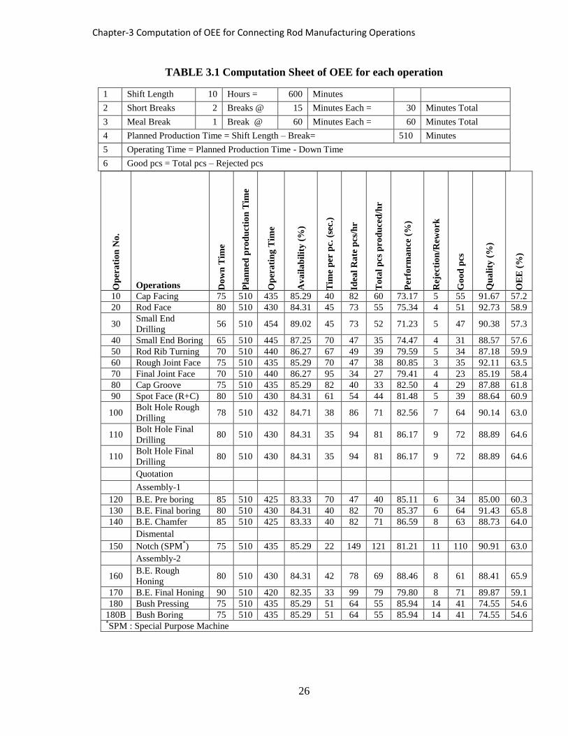
The details are prepared as shown in Table 3.1, for machining operations of a product to
compute OEE to enlighten the working environment of shop floor activities.
Chapter-3 Computation of OEE for Connecting Rod Manufacturing Operations
26
TABLE 3.1 Computation Sheet of OEE for each operation
1 Shift Length 10 Hours = 600 Minutes
2 Short Breaks 2 Breaks @ 15 Minutes Each = 30 Minutes Total
3 Meal Break 1 Break @ 60 Minutes Each = 60 Minutes Total
4 Planned Production Time = Shift Length – Break= 510 Minutes
5 Operating Time = Planned Production Time - Down Time
6 Good pcs = Total pcs – Rejected pcs
Op
era
tio
n N
o.
Operations Do
wn
Tim
e
Pla
nn
ed p
rod
uct
ion
Tim
e
Op
era
tin
g T
ime
Av
ail
ab
ilit
y (
%)
Tim
e p
er p
c. (
sec.)
Idea
l R
ate
pcs
/hr
To
tal
pcs
pro
du
ced
/hr
Per
form
an
ce (
%)
Rej
ecti
on
/Rew
ork
Go
od
pcs
Qu
ali
ty (
%)
OE
E (
%)
10 Cap Facing 75 510 435 85.29 40 82 60 73.17 5 55 91.67 57.2
20 Rod Face 80 510 430 84.31 45 73 55 75.34 4 51 92.73 58.9
30 Small End
Drilling 56 510 454 89.02 45 73 52 71.23 5 47 90.38 57.3
40 Small End Boring 65 510 445 87.25 70 47 35 74.47 4 31 88.57 57.6
50 Rod Rib Turning 70 510 440 86.27 67 49 39 79.59 5 34 87.18 59.9
60 Rough Joint Face 75 510 435 85.29 70 47 38 80.85 3 35 92.11 63.5
70 Final Joint Face 70 510 440 86.27 95 34 27 79.41 4 23 85.19 58.4
80 Cap Groove 75 510 435 85.29 82 40 33 82.50 4 29 87.88 61.8
90 Spot Face (R+C) 80 510 430 84.31 61 54 44 81.48 5 39 88.64 60.9
100 Bolt Hole Rough
Drilling 78 510 432 84.71 38 86 71 82.56 7 64 90.14 63.0
110 Bolt Hole Final
Drilling 80 510 430 84.31 35 94 81 86.17 9 72 88.89 64.6
110 Bolt Hole Final
Drilling 80 510 430 84.31 35 94 81 86.17 9 72 88.89 64.6
Quotation
Assembly-1
120 B.E. Pre boring 85 510 425 83.33 70 47 40 85.11 6 34 85.00 60.3 130 B.E. Final boring 80 510 430 84.31 40 82 70 85.37 6 64 91.43 65.8 140 B.E. Chamfer 85 510 425 83.33 40 82 71 86.59 8 63 88.73 64.0
Dismental 150 Notch (SPM
*) 75 510 435 85.29 22 149 121 81.21 11 110 90.91 63.0
Assembly-2
160 B.E. Rough
Honing 80 510 430 84.31 42 78 69 88.46 8 61 88.41 65.9
170 B.E. Final Honing 90 510 420 82.35 33 99 79 79.80 8 71 89.87 59.1 180 Bush Pressing 75 510 435 85.29 51 64 55 85.94 14 41 74.55 54.6
180B Bush Boring 75 510 435 85.29 51 64 55 85.94 14 41 74.55 54.6 *SPM : Special Purpose Machine

OEE factors and Computation sheet
27
Equations:
A. Availability =
x 100 %
B. Performance =
x 100 %
C. Quality =
x 100 % =
x 100 %
D. Overall Equipment Effectiveness = Availability x Performance x Quality
3.6 Analysis
The data sheet prepared indicates the gray area of the shop floor. There is a need to emphasize
the last manufacturing operation, i.e. bush boring and bush pressing. The quality of this
operation is lower as compared to other operations. This is because of more rework needed in
this operation to have desired quality. The team of manufacturing unit targets to improve this
aspect as it is one of the most crucial steps.
The team initiated the deep study of bush pressing and bush boring operation which includes
many parameters. The fish bone diagram prepared for this operation as shown in Fig. 3.1. The
following actions were taken and appropriate corrections implemented to have better quality at
this stage.
- Alignment (straightness) of the fixture checked and found correct.
- The spindle axial alignment checked and corrected with necessary action.
- Tool wear measured for a lot size and suggested to alter the tool change frequency as
the previous one was inadequate.
- Measuring instrument checked with master calibration unit and found correct.
Operator interviewed for his fitness to the work and asked for necessary improvement.

Chapter-3 Computation of OEE for Connecting Rod Manufacturing Operations
28
FIGURE 3.1 : Fishbone diagram showing rejection potentials
3.7 Results and discussion
The tool change frequency altered from 500 pcs to 400 pcs in bush boring operation. The
impacts of employed actions are represented in the graph. There is a reduction in variation in
the center distance parameter (Fig. 3.2 and 3.3). There is a reduction in rework (Fig. 3.4),
rejection (Fig. 3.5) and customer complaints (Fig. 3.6) for this parameter.
Bush Boring
Rejection/Rework
Small End
Drilling
Bend/Twist
Small End
Boring
Diameter of Bore
undersize/oversize
Bush Pressing
Bush axis
Bush Diameter
Bush Boring
Spindle Axis
Bush Thickness
Taper ness of
bore

Results and discussion
29
FIGURE 3.2 : Variation in Center
Distance before implementation (More
variation)
FIGURE 3.3 : Variation in Center
Distance After implementation (Less
variation)
FIGURE 3.4 : Rework % (monthly)
FIGURE 3.5 : Rejection % (monthly)
FIGURE 3.6 : Customer Complaints (monthly)

Chapter-3 Computation of OEE for Connecting Rod Manufacturing Operations
30
3.8 Limitations for using OEE system
- The percentage calculation of OEE is statistically cannot be said valid. A calculated
OEE percentage assumes that all equipment-related losses are equally significant and
any improvement in the value of OEE is a positive improvement for the whole plant.
This may not be true for all the cases. For example, the calculated OEE percentage
does not consider that two percent improvement in quality may have a bigger impact
on the business than does a two percent improvement in availability.
- Calculated OEE is not valid for benchmarking or comparing various processes, assets
or equipment. It is a relative measure of a specific single asset effectiveness associated
with it over a period of time. However, OEE can be used to compare identical
equipment in identical situations producing identical output.
- The calculated OEE cannot be used as a corporate level measure. It is just an estimated
measure of selected equipment effectiveness only.
- Also, it does not measure maintenance effectiveness because most of the loss factors
are not under the direct control of the maintainers.
3.9 Summary
OEE System identifies the problem area and accurately the symptoms of each problem.
However, the real opportunity lies in the ability to determine the root causes for each loss,
and then to implement effective corrective actions to abolish them. OEE Systems can also be
used to gather supplementary data, create and report against improvement plans/agendas, and
verify or authenticate the actions taken to resolve the issues identified.
To achieve a successful implementation and to optimize the success of an OEE System,
organizations must focus to ensure an assurance to practice it as a fundamental, organization-
wide tool to drive continuous improvement in an effective mode. OEE can be applied to
manufacturing, petrochemical processes and environmental equipment. Overall, OEE can be
visualized in a single statement as, Implementation of OEE System can be compared to

Limitations for using OEE system
31
switching on the light in a darkened chamber. Nothing has changed, but the things can be
seen more clearly.

Chapter-4 Implementation of Bush Boring Chamfer to avoid manual De-burring in connecting rod
32
CHAPTER – 4
Implementation of Bush Boring Chamfer to avoid
manual De-burring in connecting rod: A Kaizen
Approach
4.1 Introduction
Numerous organizations have adopted the practice of Kaizen as a mean for obtaining the
alternatives for continuous improvement. Many articles have addressed the implementation of
Kaizen in different industries.
The purpose of the present work is to identify and outline the application of Kaizen approach
on the shop floor of connecting manufacturing operations. After the bush boring operation, in
Small End of connecting rod, pillar drill is used to eliminate dent marks and burrs, as a
replacement for manual de-burring operation. It reduces manual work with better concentricity
of small end and improves the quality of product up to a considerable extent.
Assembly of gudgeon pin in the small end of connecting rod becomes easier as compared to
the previous method due to chamfered end. The efforts made by teamwork to employ kaizen
concept is documented and discussed in details. Future scope of present work and
supplementary improvement potential is stated which is highly significant for the people
involved in connecting rod manufacturing.
4.2 Literature Review
Kaizen in one of the most important methodologies used to manage continuous improvement
in maquiladora industry located in Ciudad Juarez, Chihuahua, Mexico; however, it is

Introduction
33
frequently implemented without obtaining the expected results. The survey was validated
using a rational validation, judge validation, and statistical validation using the Cronbach
alpha index. The result indicated that seven factors are the most important: education and
training in operators, communication process, documentation and evaluation of projects
results, human resources integration, management commitment and customer focus [37].
Management commitment and education are the main factors that guarantee the success of
kaizen implementation programs, but that is moderated by a good communication for having
good operational process performance for better workers and customer satisfaction [38].
Kaizen is a way of thinking and managing. Its essence is the continuous improvement of
processes in an enterprise through small steps performed by all employees. Processes of
implementing new ideas are more efficient when it is supported with kaizen activities. It is a
slower but permanent improvement of things, starting from simple improvements of tools and
working methods, finishing with the improvement of whole processes performed by all
employees achieved with small steps in a way that does not require considerable investments.
A continuous improvement is a tool used by Toyota production system (TPS) and is also
called kaizen. It is not only the process of fostering creativity, raising the spirit and forming
energy, but it is also the best tool for creating value problems quickly. However, the most
effective way to achieve the above is to improve endlessly and train employees to improve the
enterprise and make it the culture of the enterprise. Continuous improvement needs to form
across function groups to improve certain areas and identify the process or problem. Its
operation includes educational training, understanding problems, evaluating problems,
brainstorming, execution, standardization, achievement record, post event handling and
reporting [39].
Improving individual operation yield is an important way to increase the system yield. Studies
in this field try to stabilize the process either by finding root causes of variation and
eliminating them or by making the process insensitive to external agitations [18].

Chapter-4 Implementation of Bush Boring Chamfer to avoid manual De-burring in connecting rod
34
4.3 Research Methodology
The aim of present work is to implement the new idea to replace manual operation with
drilling machine for better concentricity and consistency. Hence, it is an Applied Research
used for a solution of an immediate problem facing an industry. The observations were taken
according to definite pre-arranged plans and involve experimental procedure. The controlled
observations data is collected and documented for analysis. Such observations have a tendency
to supply formalized data upon which generalizations can be built with some degree of
assurance [1].
In machining, the objects in quality control are geometrical dimension, tolerance, surface
finish, and relative tolerances on individual part. In mechanical assembly, the quality control
is oriented to confirm the correct relations between a group of parts or components and the
precisions with multi-dimensions, shapes, or relative position tolerances [19].
The methodology employed in present work is purely shop floor base activity. The case study
discussed for implementation, cannot be generalized for other work as it is completely Tailor-
Made Solution (TMS). It has focused on a practical description of Kaizen approach in the
production line.
4.4 Problem Statement
The product, connecting rod faced the problem of dent marks in the small end after manual de-
burring operation (Fig. 4.1) and uneasiness to insert the gudgeon pin on the small end at the
time of assembly. The solution of the problem is taken for the present case study. The scope
for improvement potential is studied and necessary corrective measures are to be taken with
the help of a kaizen approach. The present approach is checked for continuous improvement in
the ongoing process with the help of cost-benefit analysis (CBA).
The brainstorming exercise was conducted by an interdisciplinary team of engineers at the
company in order to identify potential factors that could influence the problem. The team
assessed a number of factors and proposed to add bush bore chamfering operation with pillar
drilling machine as shown in Fig. 4.2. It eliminates manual de-burring operations. The
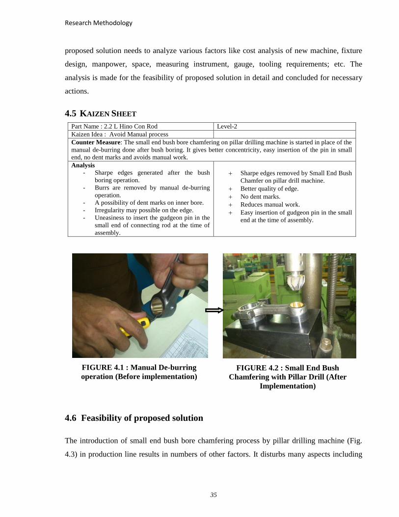
Research Methodology
35
proposed solution needs to analyze various factors like cost analysis of new machine, fixture
design, manpower, space, measuring instrument, gauge, tooling requirements; etc. The
analysis is made for the feasibility of proposed solution in detail and concluded for necessary
actions.
4.5 KAIZEN SHEET
Part Name : 2.2 L Hino Con Rod Level-2
Kaizen Idea : Avoid Manual process
Counter Measure: The small end bush bore chamfering on pillar drilling machine is started in place of the
manual de-burring done after bush boring. It gives better concentricity, easy insertion of the pin in small
end, no dent marks and avoids manual work.
Analysis
- Sharpe edges generated after the bush
boring operation.
- Burrs are removed by manual de-burring
operation.
- A possibility of dent marks on inner bore.
- Irregularity may possible on the edge.
- Uneasiness to insert the gudgeon pin in the
small end of connecting rod at the time of
assembly.
Sharpe edges removed by Small End Bush
Chamfer on pillar drill machine.
Better quality of edge.
No dent marks.
Reduces manual work.
Easy insertion of gudgeon pin in the small
end at the time of assembly.
FIGURE 4.1 : Manual De-burring
operation (Before implementation)
FIGURE 4.2 : Small End Bush
Chamfering with Pillar Drill (After
Implementation)
4.6 Feasibility of proposed solution
The introduction of small end bush bore chamfering process by pillar drilling machine (Fig.
4.3) in production line results in numbers of other factors. It disturbs many aspects including

Chapter-4 Implementation of Bush Boring Chamfer to avoid manual De-burring in connecting rod
36
costing. The initial investment in terms of machine cost and fixture cost, tool cost, manpower
cost, space utilization, measuring instrument, etc are justified to the management. The fixture
is prepared for the proposed action plan as shown in Fig. 4.4. The implemented action shows
improvement in the quality of small end bush bore. It shows the reduction in customer
complaint due to easy insertion of gudgeon pin in the small end at the time of assembly of the
piston and connecting rod at the customer end. The assembly line also reported the reduction
in assembly time due to implemented action.
FIGURE 4.3 : Pillar Drilling machine
FIGURE 4.4 : Fixture for implemented action

Concluding Remarks
37
4.7 Concluding Remarks
The purpose of this chapter is to describe the implementation of continuous improvement in
connecting rod manufacturing operation. The kaizen approach presented shows improvement
in quality in terms of many aspects. The dent marks in the small end are eliminated and
assembly of pin becomes faster and easier as compared to the previous method. Further
research in this area will need to focus on the practical experience of other aspects of other
manufacturing operations.
Indeed, the concept of kaizen is outstanding road-maps, which could be used in order to
strengthen the practices within an organization. Even if some of the other concepts have been
accused of being management trends, it is the authors’ interpretation that organizations
continuously need to work with customer-orientated activities in order to survive; irrespective
of how these activities are labeled today and in the future.

Chapter-5 To Control variation in End Float Parameter with the Application of Six Sigma Tools
38
CHAPTER – 5
Control Variation in End Float Parameter with the
Application of Six Sigma Tools
5.1 Introduction
Six Sigma tools are widely used by a number of reputed industries to solve the burning issues
of the shop floor. The manufacturing of product involves the number of operations, quality of
which affects the quality and performance of the final product. There is a scope to interrelate
these operations’ quality and their effect on the final product. The control of the operations at
individual stages results in better outcome. This chapter proposes the proper implementation
of various Six Sigma tools to solve the longer existed problem named as End Float of
connecting rod.
5.2 Literature review
The number of companies has developed and implemented Six Sigma approaches. At
Samsung, Six Sigma projects usually focus on either redesigning processes and systems or
improving performance levels of existing systems [40]. Honeywell is known for the extensive
application of lean methodologies, which has become a major tool in their Six Sigma
implementation. Honeywell developed a proprietary Six Sigma approach called Six Sigma
Plus which links lean manufacturing concepts and tools [41].
A key element of General Electric’s approach to Six Sigma is tailoring underlying
methodologies to specific needs and characteristics of its business units. The company has
taken the generic Six Sigma methodology for process innovation and has tailored their specific
needs of system design and implementation as well as product development activities.

Introduction
39
Six Sigma Quality quantitatively means that the average review process generates 3.4 defects
per million units – where a unit can be anything ranging from a component to a line of code or
an administrative form. This implies that nearly flawless execution of key processes is critical
to achieving customer satisfaction and productivity growth [42]. The Six Sigma initiatives in
TCS-GEDC (The Global Engineering Development Center of Tata Consultancy Services)
started in 1998, and, since then, 11 Six Sigma projects have been completed and five are in
progress. These projects include Improvement of Schedule Compliance, Quality Compliance,
Input Quality, Error Reduction, Cycle Time Reduction and Design Improvement.
Motorola was the first company to launch a six sigma program in the mid-1980s. In 1988,
Motorola received the Malcolm Baldrige National Quality Award, which led to an increased
interest of six sigma in other organizations. Today, a number of global organizations have
developed six sigma programs of their own and six sigma is now established in almost every
industry [21]. Six sigma could also be described as an improvement program for reducing
variation, which focuses on continuous and breakthrough improvements. Improvement
projects are driven in a wide range of areas and at different levels of complexity, in order to
reduce variation. The main purpose of reducing variation on a product or a service is to satisfy
customers.
Six Sigma is a tool which is widely used in the industrial and service organizations to enhance
quality and reduce costs. The concepts are also applicable to distance education with certain
modifications [43].
In the process of mechanical assembly, the assembly relationship in orientation, position,
geometrical dimensions, and matching between parts and components should be built first,
and these relations should be in accordance with the design requirements. The objectives of
quality control (QC) in mechanical assembly can be considered to match the product design in
the logical relationship between parts and components, and the precisions of geometric
relations. The unstable factors and their variation existing in the assembly process may lead to
high risk of serious quality problems and make the objects of assembly quality assurance out
of specifications [44]. The quality problems can be categorized as the logical relationship
failure, precision failure, and non-technical failure [45].

Chapter-5 To Control variation in End Float Parameter with the Application of Six Sigma Tools
40
In machining, the objects in quality control are geometrical dimension and tolerance, surface
finish, and relative tolerances on individual part. In mechanical assembly, the quality control
is oriented to confirm the correct relations between a group of parts or components and the
precisions with multi-dimensions, shapes, or relative position tolerances [19]. So the relative
regulations and methods should be employed in mechanical assembly.
The quality of the final products highly depends on the quality of assembly operations and
process [46]. However, the mistakes and errors in assembly processes are high sources of
defects and erode margins of products. So some valuable theoretical models and technological
measures have been brought forward based on the researches in this area recently. An
algorithm is presented to propagate and control variation in mechanical assembly of
automobile assembly by the state transition model approach [47].
Normal process variations are divided into common variation and special variation [48].
Common variation mainly arises from common causes, which is also called chance or random
variation. It involves a different view of factors in an in-control process. In a manufacturing
process, raw material lot-to-lot variability and operator-to-operator variability are the likely
common causes. In a business process, day-to-day variability and department-to-department
variability are more likely to be considered as the common causes [39]. The Special variation
comes from non-human factors, such as the wear and tear of tools, lack of adjustment in
equipment, bad quality material etc., or human factors, such as negligence, tiredness and
incorrect operation. This is also called assignable variation.
5.3 Six Sigma frame work
Mathematically Six Sigma represents six standard deviations (plus or minus) from the
arithmetic mean. As a measurement of quality Six Sigma means the setting of a performance
level that equates to no more than 3.4 Defects Per Million Opportunities (DPMO) or 3.4 defect
Parts Per Million (PPM) Opportunities. Six Sigma is an approach that takes a whole system
approach for improvement of quality and customer service so as to benefit the ‘bottom line’.
The Six Sigma concept matured during the mid-eighties and grew out of various quality
initiatives. Like most quality initiatives Six Sigma requires a total culture throughout an

Six sigma frame work
41
organization whereby everyone at all levels has a passion for continuous improvement with
the ultimate aim of achieving virtual perfection. To know if Six Sigma has been achieved
needs a common language throughout the organization (at all levels and within each function)
and common uniform measurement techniques of quality. The overall Six Sigma philosophy
has a goal of total customer satisfaction [49].
Six Sigma is an organized structure to diminish variation in organizational processes by using
improvement specialists and performance metrics with the aim of attaining strategic
objectives. Companies may choose variations of this base definition when implementing Six
Sigma in order to customize it to their situation. Contingency theory implies that the base
definition will not fit every company, but nonetheless, it is a starting point for research and
implementation [50].
‘Six Sigma is an organized and systematic method for strategic process improvement that
relies on statistical methods and the scientific method to make melodramatic cutbacks in
customer defined defect rates’. The simplest definition for Six Sigma is to eliminate waste and
to mistake proof the processes that create value for the customer. The elimination of waste led
to yield improvement and production quality; higher yield increased customer satisfaction.
A model which correlates the interrelationships of the factors affecting the quality of the
product as discussed in the brainstorming session and shown in fishbone diagram need to be
prepared for continuous improvement of the product quality. The approach is proposed for the
allocation of tolerance to different parts, to minimize the manufacturing cost and satisfy the
assembly function [51] [52].
The optimization objectives and constraints for concurrent tolerance design for manufacture
and assembly are discussed, and the key technologies for concurrent tolerance design with
game theory are investigated, including the strategy set division, payoff calculation, and Nash
equilibrium evolution [53].

Chapter-5 To Control variation in End Float Parameter with the Application of Six Sigma Tools
42
5.4 Problem Statement
The organization studied was an SME based in Rajkot, Gujarat, dealing with the
manufacturing of various auto parts of Compression Ignition Engine. The product connecting
rod faced the problem of End Float for a very long time. The problem was taken for the
present case study. The scope for improvement potential was to be studied and necessary
corrective measures were to be taken with the implementation of Six Sigma tools.
5.4.1 Meaning of End Float
Normally, the thickness of the rod face and cap face is same in connecting rod but in some
design of the connecting rod, there is the difference in the thickness of rod and thickness of the
cap. In the big end face of connecting rod, the cap is assembled with nuts and bolts. The
thickness of big end face of connecting rod is more than the thickness of cap face. Due to the
difference in the thickness, there is a gap between the planes of rod face and cap face. The gap
needs to be maintained half on both the sides of the connecting rod. This is called as End Float
of connecting rod as represented in Fig.5.1.
5.4.2 Computation sheet of End Float
Mathematically, End float can be calculated as shown in Table 5.1. Lower dimension and
Upper dimensions of Rod’s face and Cap width decides the value of End Float. The maximum
and minimum values of this parameter occur in extreme conditions of Rod face width and Cap
width.
TABLE 5.1 : Computation Sheet of End Float
Parameter Lower Dimension
A (mm)
Upper Dimension
B (mm)
Mean
(mm)
Range
(b-a)
(mm)
Rod face width R 39.375 39.434 39.4045 0.059
Cap width C 38.230 38.480 38.355 0.250
Total Difference ( Rmin - Cmin ) 1.145 - - -
Total Difference ( Rmax - Cmax ) - 0.954 - -
Total Difference ( Rmin - Cmax ) 0.895 - - -
Total Difference ( Rmax - Cmin ) - 1.204 - -
Total Range of End Float 0.895 1.204 - -
One side difference 0.448 0.602 0.52475 0.154

Problem Statement
43
All dimensions are in mm
Not to scale
FIGURE 5.1 : End float of connecting rod (diagrammatic presentation)
5.5 DMAIC:
The project team followed five phases and key tools used in each phase are as listed bellow:
1. Define: Pareto Analysis; Project Charter.
2. Measure: Descriptive Statistics; Process Capability Analysis.
3. Analyze: Detailed Process Map; Fish-Bone Diagram.
4. Improve: Experimentation; New Process.
5. Control: Statistical Process Control.
The five Six Sigma phases (Define, Measure, Analyze, Improve and Control) are discussed in
details (Fig. 5.2).

Chapter-5 To Control variation in End Float Parameter with the Application of Six Sigma Tools
44
FIGURE 5.2 : Six Sigma Process
5.5.1 Define Phase
This is the first phase in Six Sigma project. This phase is defined by the following questions.
1. Who are the customers and what are their priorities?
2. Where are their problems?
3. Which do we attack first?
The subsequent process is the customer of the earlier process. The product or process to be
improved is identified and recognized. Customer needs are identified and translated into
Critical to Quality Characteristics (CTQ’s). The problem or goal statement, the project scope,
the role of team members and milestones are developed. A high-level process is mapped for
the prevailing method. It also uses Pareto analysis to identify and prioritize projects that will
be worked on as part of continuous improvement process in the company.
Pareto Analysis: The manufacturing of connecting rod includes many machining operations.
After a long study, the major quality problems related to connecting rod manufacturing is
studied and the database is prepared for various problems. The company has done excellent
continuous improvement program for the manufacturing of various automobile components to
be manufactured in a very large quantity. The company is now starting to look at the tools
available in Six Sigma process to further its continuous improvement efforts.

Return on quality
45
There are many parameters to be controlled for achieving the quality of a product. The
connecting rod manufacturing includes nearly 23 manufacturing operations. All the operations
need to have proper attention for a quality product. A little deviation of one parameter at the
early stage may cause higher deviation of other parameter/s at later stages. This product (i.e.
connecting rod) is also having a number of parameters to be controlled within the specified
limit, not be rejected at any stage. Hence, the database of major rejection parameters is
prepared and the possible causes for the same need to be analyzed.
The Pareto chart shows the top seven rejection parameters of connecting rod Fig. 5.3. It
indicates that the major rejection of the connecting rod occurs because of big end bore
diameter variation. The second major problem of bolt tight is raised in the current year and the
third one, i.e. end float has existed for many years and should be significantly decreased, if not
eliminated. Due to the second major problem, the functionality of the component is not
affected but the problem occurs at the time of assembly of the engine.
Once the assembly is prepared, the problem gets nullified whereas the third one causes the
functional problem of the engine. Because of the end float, it was noticed by the customer that
there is a significant increase in the frictional power loss. Hence, the area of focus for this
project is the issue of end float of the connecting rod.
5.3 : Pareto Chart
280
140
80
36 36 30 2418
0
50
100
150
200
250
300
Bore
Dia
Bolt T
ight
End F
loat
Bend
Tw
ist
Notc
h S
ides
Wro
ng C
entr
e
Dis
tance
Oth
ers
0
20
40
60
80
100
120
140
160
180
Rejection Qnty
Cumulative %

Chapter-5 To Control variation in End Float Parameter with the Application of Six Sigma Tools
46
It is the goal of the project team to eliminate the cause of the top three quality issues in each
area on an annual basis. So over the multiple years, the majority of the quality issues can be
solved.
5.5.2 Measure
The key internal processes that influence the CTQs (Critical to Quality) are identified and the
defects generated relative to the identified CTQs are measured. It helps in creating the
capability of given process and ascertaining existing performance levels. The objective of the
measurement stage is to find out the magnitude of the problem and collect data to discover the
few vital root causes. At this stage cause and effect relationships should be established. During
the measurement process, the critical to quality (CTQ) characteristics which have an impact
on the outcome would be selected.
The quality issue selected for the present work is End Float, which refers to maintain the gap
between the plan of the connecting rod face and cap face in the final assembly of the
connecting rod. The issue of End Float accounted for 20 % of the quality issues. It is measured
for each part using a set of filler gauge. The big end rod face was supported on the surface
plate and gauge passed from the gap between rod face and the surface table. The dial indicator
arrangement can also be done for end float measurement. The difference between the dial
reading taken at rod surface and cap surface indicates double the value of the end float. The
second method is lengthy as compared to the first method as it uses only filler gauge.
The parameter End Float is affected by many manufacturing operations. Hence, to maintain
this parameter within the required range, it is required to look after many manufacturing
operations. A single control activity can’t control the multiple correlative manufacturing
operations in the process. So the logical relations of control activities should be considered,
and the united control activities should be carried out. The quality control activities usually
include checking the conformity of quality characteristics against inspection specification,
collecting and recording sampling data, monitoring the state of process characteristics, and so
on.

Return on quality
47
5.5.3 Analyze
The objective of this phase is to understand why defects are generated. Brainstorming and
statistical tools are used to identify key variables (X’s) that cause defects. The output of this
phase is the explanation of the variables that are most likely to affect process variation. The
data is analyzed to find out the potential sources of variation and reduce the number of process
variables to be acted on in the improvement phase. This is the stage at which new goals are
set, and the route maps created for terminating the gap between current and target
performance. The analysis also includes identifying root causes and arranged areas for
improvement.
The brainstorming exercise was conducted by an interdisciplinary team of engineers at the
company in order to identify potential factors that could influence the problem of end float.
The team assessed a number of factors and finally reduced them to five key factors. The key
factors are shown by fishbone diagram in Fig. 5.4. Following are the main factors which affect
this problem.
1. Misalignment of the bolt hole axis.
2. Higher or lower widths of the rod during Rod face grinding operation.
3. Cap facing operation towards extreme dimension.
4. Taper-ness of rod face and cap face higher than the allowable limit.
5. The distance between the center of the bolt hole and the face of rod/cap out of
allowable limit.

Chapter-5 To Control variation in End Float Parameter with the Application of Six Sigma Tools
48
FIGURE 5.4 : Cause and Effect Diagram for End Float
5.5.4 Improve
The objective of this phase is to confirm the key variables and quantify the effect of these
variables on the CTQs. It also contains identifying the extremely acceptable ranges of the key
variables, confirming the measurement systems and modifying the existing process to stay
within these ranges. This is the stage where the root cause of the problem is removed and the
corrective actions are standardized. The proposed solutions are confirmed and implementation
strategy is worked out. To ensure that the corrective actions are effective, they are tried out in
a prototype before commencing on concluding improvement. This is the stage where the
ground work is translated into action. The output is measured continuously to monitor the
extent of improvement along the CTQ parameters.
Taper
Rod Face Grinding
Oversize/
Undersize
Rod face taper more
than allowable limit
Oversize
Bolt Hole Drilling
End Float Out
of Limit
Miss alignment
of axis
Cap Facing
Cap face taper more
than allowable limit
Undersize Higher/Lower Bolt
Hole Center
Distance from Face

Return on quality
49
The five major key variables listed above are analyzed for rejected components. The majority
of the rejection took place because of the distance between the center of the bolt hole and the
rod face. It was noticed that this distance measured higher on one side and lower on another
side. To study the possible reason for this cause, the fixture of the bolt hole drilling machine
needed to be inspected.
The fixture of the bolt hole drilling machine checked for a number of parameters which
includes surface roughness, taper-ness, the distance between locators of small end bore and
big end parting face and vibration possibilities during the machining operation.
For drilling operation, the big end face of the rod was located on the surface of the fixture. It
was observed that the surface of the fixture used in drilling operation was tapered. This taper-
ness came into effect only when extreme conditions match. When the taper ness of rod co-
insides with the taper-ness of the fixture plane, the ultimate effect of the taper-ness on the rod
drilling nullifies or reduces. When the taper-ness of rod and fixture plane become of the same
type, then the combined effect increased up to the considerable amount.
The linear diagram is shown in Fig. 5.5. The possibility of this occurrence looks to be little,
but it does matters for the studied rejected components.
FIGURE 5.5 : Taper ness of Big End Face of Rod and Surface of Fixture (Not to scale)
There are two possible corrective measures to overcome the problem. The first one is to alter
the fixture plate which is tapered as shown in Fig. 5.6. The second is to ensure that the taper-
ness of the rod must co-inside with the taper-ness of the fixture plane. This can be performed
by measuring the taper-ness of the rod face by dial indicator and locating the rod face
a. Both taper planes co insides
(Cumulative effect reduces taper ness)
b. Both taper planes are of same kind
(Cumulative effect increases taper ness)
R : Rod face of Big End F : Fixture surface
a
a
b
R
R
F F

Chapter-5 To Control variation in End Float Parameter with the Application of Six Sigma Tools
50
accordingly on the fixture locator. The second solution is to be adopted locally for the
temporary solution. Hence, there is a need to alter the taper-ness of fixture either by fully
changing the fixture or providing the packaging to the tapered side.
FIGURE 5.6 : Fixture alteration proposed for solution
5.5.5 Control
In the control stage, the new process – conditions are documented and incorporated into
systems so that the improvements remain sustained. Hence, the objective of this phase is to
ensure that the modified process now enables the key variables to stay within the maximum
acceptable range, using tools like Statistical Process Control (SPC) or control charts or simple
checklists.
The control plan is composed of quality control activities in each manufacturing operations.
The control essence is that different activities that have the different effect on manufacturing
quality are controlled by different control tactics and measures. It is needed to execute a very
long exercise when this parameter deviates from its mean value. There are many techniques to
measure these parameters which include the usage of filler gauge. The GO and NO GO
concept is used to check whether the parameter is within the limit or not.
The fixture of the bolt hole drilling machine changed and the tolerance for the taper-ness for
the fixture plane redesigned and calculated for an extremely tapered face of the rod. After
Return on quality
51
implementing the new fixture, a batch of the products taken for machining operation and
extremely tapered rod faces taken for bolt hole drilling. The end float of the rods with tapered
faces measured which found to be within the allowable limit. A checklist for fixture inspection
prepared and the new taper-ness allowances checked for the control of the process.
5.6 Return on quality
In order to change the fixture, it must be determined that the benefits from the newly designed
fixture outweigh the costs. Assuming the new fixture achieves the intended goals, the rejection
due to end float reduced up to 20% of total rejection quantity and 0.8 % of the total production
quantity. The savings will be recognized on approximately 10000 parts per month which
equate to a monthly savings of (Rs. 10000x0.8x250=) Rs. 20000 and annual savings of Rs.
240000. The cost of new fixture is Rs. 5000/- which is to be recovered within a period of less
than one month of the time.
5.7 Conclusion
It is recommended that the company move forward with the new fixture design. It is also
recommended that the company implement a checklist to monitor the amount of taperness of
the new fixture plane. The thrust on Six Sigma Quality has helped in creating and sustaining
customer focus in the company leading to improved customer satisfaction as indicated in the
feedback from the customer. At the same time, active participation of the team members from
all levels in the Six Sigma projects has evolved a culture of effective and creative team work.
This project has demonstrated the power of six sigma process to solve the problems that
appeared unsolvable. The company had been suffering from the problem of end float for very
long years. The corrective actions to be identified, tested and ready for implementation.
The end float problem to be resolved by altering the taperness of the fixture plane which
locates the big end rod face. The second solution discussed, can also be implemented if the
taperness value of the fixture plane checked higher than the newly designed tolerance.

Chapter-5 To Control variation in End Float Parameter with the Application of Six Sigma Tools
52
The quality of the final product should not merely rely on the general inspections due to the
complexity of unstable factors in manufacturing process. The errors or variation caused by
those factors could be accumulated gradually in the process and thus avoid serious troubles in
the following stages.
The six sigma process is an excellent fit for the fabrication and machining industries. It is
implemented in present case with structured approach. Any company that needs solutions for
quality related problems should benefit from this process. Companies will be most likely to
succeed if their top-level management is supportive of a continuous improvement culture.
Companies should also choose projects that can be measured and that potentially have a good
return on quality.

Theoretical Background
53
CHAPTER – 6
Quality Assurance of Axial Mis-alignment (Bend and
Twist) of Connecting Rod
6.1 Introduction
The connecting rod is the intermediate member between piston and crankshaft. Its primary
function is to transmit the push and pull from piston pin to crank pin. Thus it converts the
reciprocating motion of a piston into the rotary motion of crank. These are generally
manufactured by a drop forging process. The small end is lined with a gun metal bush. The
brasses in the big end are of C.I. or Cast Steel and are lined with white metal. Main parts of
Connecting rod are Rod, Cap, Nuts (2 Nos.), Bolts (2 Nos.) and small end bush shown in
Fig.6.1.
6.2 Theoretical Background
Forces acting on the connecting rod
1. Force on piston due to gas pressure and inertia of the reciprocating parts.
2. The force due to the inertia of connecting rod (Inertia bending force).
3. The force due to the friction of the piston rings and of the piston.
4. The force due to the friction of the piston pin bearings and crank pin bearing.

Chapter-6 Quality Assurance of Axial Mis-alignment (Bend and Twist) of Connecting Rod
54
FIGURE 6.1 : Connecting Rod assembly with press fitted brass bush, Cap, Nuts and
Bolts
The connecting rod is considered as column pillar as it is subjected to cyclic compressive and
tensile load which is acting in an axial direction. During the suction stroke, the rod is
subjected to the partial tensile load. During the compression stroke, the rod is subjected to the
partial compressive load. When power stroke occurs, again the rod is subjected to high
compressive load and during exhaust stroke; a small amount of compressive load is there. So
cyclic loading occurs with the connecting rod. For the design consideration, compressive
failure should be considered which occurs during power stroke as it is higher as compared to
other three strokes.
1. The connecting rod is subjected to alternating direct compressive and tensile forces.
2. Compressive forces are much higher than tensile forces; so cross section of connecting
rod is designed as strut and Rankine’s formula is used.
Due to axial load, the rod may buckle as shown in Fig. 6.2 and Fig. 6.3. Consider, the
connecting rod as both the ends hinged about X axis for buckling and both ends are fixed
about Y axis for buckling.

Theoretical Background
55
FIGURE 6.2 : Buckling of Connecting Rod about Y-axis (Both ends fixed Leq = l/2)
FIGURE 6.3 : Buckling of Connecting Rod about X-axis ( Both ends hinged Leq = l )
According to Rankine’s formula,
WB about X axis =[ σc x A ] / [ 1 + a { Lequ / Kxx }2 ] , for Leq = l ; both ends hinged. (1)
WB about Y axis = [ σc x A ] / [ 1 + a { Lequ / Kyy }2 ], for Leq = l/2 ; both ends fixed. (2)
Where, Leq = Equivalent length of connecting rod.
a = Rankine’s constant =
for C.I.
=
for M.S.
=
for Wrought Iron
To have an equal strength of connecting rod in buckling about both axis, the buckling load
must be equal.
i.e.
=
=
Kxx 2 = 4 Kyy
2
Ixx = 4 Iyy (3)
Hence, connecting rod is 4 times stronger in buckling about Y axis than about X axis.
If Ixx < 4 Iyy then buckling will occur about X axis.

Chapter-6 Quality Assurance of Axial Mis-alignment (Bend and Twist) of Connecting Rod
56
if Ixx > 4 Iyy then buckling will occur about Y axis.
Connecting rod is designed for Ixx = 3 to 3.5 Iyy (it is designed for buckling about X axis.) for
this condition, the most suitable cross section is I section, as discussed below.
Ixx = [4t x (5t)3] / 12 - [3t x (3t)
3/12 = 419 x t
4 / 12
Iyy = [5t x (4t)3]/ 12 - [3t x (3t)
3]/12 = 131 x t
4 / 12
Ixx = 3.2 Iyy (4)
FIGURE 6.4 : I-section of Connecting Rod
Dimensions of I section is decided by considering the buckling of the connecting rod about X
axis as shown in Fig. 6.4 (Both ends hinged).
6.3 Bend and Twist of Connecting rod and its measurement methods
Bend and Twist are defined as the angular misalignment of the two axes of the connecting rod
that is the axis of big end diameter and the axis of small end diameter. Both the axis should be
completely parallel in all three views. Because of manufacturing limitations, some
misalignment is tolerated up to the allowable limit. Measurement of Bend and Twist is
specified in terms of θbend and θtwist as shown in Fig. 6.2. The misalignment in Front View, as
shown in Fig. 6.2 is defined as Bend and the misalignment in Side View is defined as Twist of
connecting rod. These parameters are measured on the shop floor in terms of mm (generally,
micron) per mm of length.
There are many methods to measure Bend and Twist of connecting rod. Each method is
having its own benefits and drawbacks. At this point, four methods are discussed to measure
these parameters.

Bend and Twist of Connecting Rod and it’s measurement methods
57
6.3.1 Method 1: To measure Bend and Twist with two pins
The pin is inserted in both the ends of connecting rod. The diameter of both the pins is equal
to the mean diameter of big end and small end. The length of both the pins is longer than the
thickness of the connecting rod ends. The extended length of the pin is used to take readings.
The big end pin is to be held on the V block, and small end pin remains free in the small end.
With the help of the height gauge, readings of the big end pin are taken and the difference is
noted down as the reading D1. Because of the straightness of the pin, and V block, generally
D1 value is zero. Then after the reading of the free end of the small end pin is taken. The
difference is noted down as the reading D2. The difference of D1 and D2 indicates the
misalignment of the axis of the rod ends.
This method requires two pins of diameters equal to the diameter of the ends. The limitation of
this method is also there. The measurement done by this method consumes more time and
good skill is required for measurement. The problem of scratch marks in the inner bore of the
rod ends is possible while inserting the pins in the rod ends. It also requires skill and practice
to insert the big end pin in the big end bore which may be tightened at the time of insertion of
the pin in the big end.
Also, two pins of specified diameters are required, which can be used for this diameter bore,
only. So initial investment required is more as compared to other methods. It is also not
advisable to use this method for single piece measurement, as two pins would not be useful for
any other purpose. This method is suitable where mass production is there and sampling
inspection is carried out. It takes nearly two minutes to measure one piece by a trained and
skilled inspector. This method is much accurate, as it directly measures misalignment between
two axes; whereas other methods consider some reference planes.
6.3.2 Method 2: To measure Bend and Twist with V-block
This method is quicker and easier than others. The rod big end face is held on V block. Small
End is free in the air in an upward position. After holding big end face on V block, the pointer
of height gauge is moved in small end bore from one face to another face. The deviation in

Chapter-6 Quality Assurance of Axial Mis-alignment (Bend and Twist) of Connecting Rod
58
pointer reading indicates the value of misalignment of the axis. By shifting connecting rod
position from vertical to horizontal, the twist can be measured.
In this method, the big end face is taken as reference. Bend and Twist measured by this
method may differ from other methods. Taper in big end face is counted in this method. So
measured value is not accurate, but the difference in the readings is very small. This method is
widely used for mass inspection as it does not require greater skill and the measurement
process is much faster.
This method uses only conventional measuring devices and no need to use the pin or any other
special purpose gauges. Another advantage as compared to the first method is that there is no
any problem like scratch marks in bore because the pin is not required to be inserted in any
end. Only pointer of height gauge dial moves along the bore which does not make any scratch
marks inside the bore. The honing pattern can also be maintained inside the bore which may
be disturbed due to insertion of the pin.
This method can be used for continuous inspection also which is an added advantage.
6.3.3 Method 3: Measurement with Co-ordinate Measuring Machine
CMM can be used to measure these parameters. The connecting rod is held on CMM table and
the pointer is moved in both the bores. The pointer picks up four or five points in one plane
and another four or five points in another plane. By considering these points, it creates a
cylindrical shape based on input points. After defining the cylinder, it locates the axis which is
the axis of big end bore. Same way small end bore axis is also defined by defining the small
end bore cylinder. The parallelism of both the axis is calculated by programming of CMM and
misalignment in Front View indicates bend and misalignment in Side View indicate twist.
Parameters measured by this method are highly accurate. This method considers big end and
small end bore as references. Taper-ness of big end face does not affect the values of bend and
twist. This method also requires good skill. Only well-trained inspector can do measurement
by this method. The initial investment is also higher as CMM is the precise and costly
instrument.

Bend and Twist of Connecting Rod and it’s measurement methods
59
a. Measurement with Co-ordinate Measuring Machine
.
b. Measurement with single pin and
height gauge
c. Measurement with Special Purpose
Gauge
FIGURE 6.5 : Measurement of bend and twist of connecting rod
This method can’t be used for mass inspection. Only one or two components can be inspected
per batch production. It also takes more time as compared to 2nd
method. Only additional
advantage of using this method is that it also measures many other parameters simultaneously.
CMM also measures big end diameter, small end diameter, ovality of both the bores in upper
plane and lower plane, the center distance between two ends along with bend and twist.

Chapter-6 Quality Assurance of Axial Mis-alignment (Bend and Twist) of Connecting Rod
60
6.3.4 Method 4: Measurement with Special Purpose Gauge
Special purpose gauge can be used to measure various parameters of connecting rod. This
gauge may have a mechanical sensor or a pneumatic sensor. In mechanical sensors, movement
of pointer decides the size of the bore and in the pneumatic sensor, the pressure difference is
calibrated and it decides the dimensions.
This method can be used for mass inspection. The accuracy and precision of this method are
also very good and there is no need of having the skilled manpower in this method. The
inspection time is also lesser as compared to other methods.
Only single drawback of this method is that it requires higher initial investment. The gauge
designed for the inspection of the connecting rod cannot be used for inspection of other
components of different dimensions.
During Bush boring operation, care is taken to control bend and twist of the connecting rod.
Xavg and R charts are prepared for continuous monitoring of the parameters. With the help of
this graph, the trend of the process can be obtained and quality can be assured.
6.4 Interpretation of readings and proposed Action Plan
The Statistical Process Control is carried out for the critical parameters of the connecting rod
in order to maintain and assure the dimensional quality. The study is carried out by taking the
reading for a particular parameter while the machining operation is going on. The sequential
readings are to be taken and noted down in the format. Then after the average range Ravg and
the average of all the readings is to be calculated i.e. Xavg. The formula to calculate the value
of Cp and Cpk are as follows.
Xavg =
Range R = X max – X min
Average Range Ravg =
Upper Control Limit for X is UCLx = + A2 x
Lower Control Limit for X is LCLx = Xavg – A2 x

Process Capability Study Report
61
Upper Control Limit for Range UCLR = D4 x
Lower Control Limit for Range LCLR = D3 x
From SPC manual the value of A2, D3 and D4 to be taken. The values are as follows
A2 = 0.73, A3 = 2.06, D3 = 2.28, D4 = 0.00, σ =
Cp =
Cpk =
and Cpk =
Cp and Cpk are process capability indices. Cp represents the potentiality of the process to be
capable of the production and Cpk represents whether the process is under the statistical
control or not.
UTL is Upper Tolerance Limit and LTL is Lower Tolerance Limit specified in the drawing by
the customer.
There are two values of Cpk. We have to consider only the lower value. It indicates that how
much the process deviates from the mean value. If the process is shifted towards the UCL the
value of one Cpk will be higher and value of another Cpk will be lower. Same is true for the
opposite case. So the process should remain near to the mean.
6.5 Process Capability Study Reports

Chapter-6 Quality Assurance of Axial Mis-alignment (Bend and Twist) of Connecting Rod
62
TABLE 6.1: Process Capability Study Report for Bend
PART NAME: Con Rod INSTRUMENT USED: V Block, Pins, Height Gauge
PART NO.: LEAST COUNT: 0.001 mm
CUSTOMER NAME: M/s. Simpson M/C NO.: 17-08-00
OPERATION NAME: Small End Bush Boring MACHINE NAME: Profitech
PARAMETER: Bend OPERATOR NAME: Nayan Sahu
DATE: STUDIED BY : Sunil
SUB-
GROUP 1 2 3 4 X R
1 -0.001 0.001 0.000 -0.001 0.000 0.002 X 0.0010 CONTROL LIMITS: INTERPRETATION
2 0.000 -0.001 0.002 -0.001 0.000 0.003 R 0.0021 UCLX 0.0025 Cp<1.00
3 0.001 0.002 0.001 -0.001 0.001 0.003 UTL 0.0100 LCLX -0.0005 1. Process is not capable
4 0.004 0.003 0.005 0.004 0.004 0.002 LTL 0.0000 UCLR 0.0047 -try to shift the job to
5 -0.004 -0.003 -0.002 -0.001 -0.003 0.003 0.00100 LCLR 0.0000 another process with
6 0.004 0.003 0.005 0.003 0.004 0.002 Cp 1.6613 A2 D4 adequate capability
7 0.004 0.004 0.003 0.002 0.003 0.002 Cpk 2.9792 0.73 2.28 -try to improve capability
8 0.004 0.003 0.004 0.003 0.004 0.001 1.6700 Cp=1.00
9 0.003 0.005 0.003 0.004 0.004 0.002 1. Process is just capable
10 -0.002 -0.003 -0.004 -0.003 -0.003 0.002 Comments (If any): Cp>1.00
11 0.004 0.003 0.004 0.004 0.004 0.001 1. Process is quite capable
12 0.001 0.003 0.001 0.001 0.002 0.002 Cp>1.67
13 -0.003 -0.003 -0.005 -0.005 -0.004 0.002 1. Process is capable
14 0.001 0.002 0.003 0.002 0.002 0.002 Cpk<1.67
15 -0.002 0.000 -0.001 -0.001 -0.001 0.002 1. Machine setting required
JAN FEB MARCH APRIL MAY JUNE JULY AUG SEP OCT NOV DEC
Cp 1.70 1.77 1.83 1.90 1.70 1.71 1.66
Cpk 1.690 1.700 1.750 1.840 1.690 1.670 1.670
RESULTS
PROCESS CAPABILITY STUDY REPORT
READINGS
1.50
1.60
1.70
1.80
1.90
2.00
JAN FEB MARCH APRIL MAY JUNE JULY AUG SEP OCT NOV DEC
Cp
/Cp
k
Month
Cp/Cpk continuous Monitoring
Cp

Process Capability Study Report
63
Table 6.2 : Process Capability Study Report for Twist
6.6 Discussion of implemented action
The value of Cp and Cpk should be more than 1.66 in order to assure the dimensional quality.
If the value of Cp < 1.00 the process is not capable for the production. Try to shift the job to
another process with the adequate capability or try to improve capability.
If the value of Cp = 1.00 the process is just capable for the production.
If the value of Cp > 1.00 the process is quite capable.
If the value of Cp > 1.67 the process is perfectly capable for the production to be carried out.
If the value of Cpk < 1.67 there is a requirement of the machine setting and fixtures to be
modified.
PART NAME: Con Rod INSTRUMENT USED: V Block, Pins, Height Gauge
PART NO.: LEAST COUNT: 0.001 mm
CUSTOMER NAME: M/s. Simpson M/C NO.: 17-08-00
OPERATION NAME: Small End Bush Boring MACHINE NAME: Profitech
PARAMETER: Twist OPERATOR NAME: Nayan Sahu
DATE: STUDIED BY : Sunil
SUB-
GROUP 1 2 3 4 X R
1 -0.002 -0.003 0.001 0.001 -0.001 0.004 X 0.0014 CONTROL LIMITS: INTERPRETATION
2 0.003 0.002 0.002 0.002 0.002 0.001 R 0.0021 UCLX 0.0029 Cp<1.00
3 0.003 0.002 0.005 0.005 0.004 0.003 UTL 0.0100 LCLX -0.0001 1. Process is not capable
4 0.002 0.005 0.003 0.003 0.003 0.003 LTL 0.0000 UCLR 0.0047 - try to shift the job to
5 -0.002 -0.003 -0.002 -0.002 -0.002 0.001 0.00100 LCLR 0.0000 another process with
6 0.001 0.002 0.002 0.002 0.002 0.001 Cp 1.6613 A2 D4 adequate capability
7 0.002 0.003 0.003 0.002 0.003 0.001 Cpk 1.8700 0.73 2.28 -try to improve capability
8 -0.005 -0.002 -0.003 -0.003 -0.003 0.003 1.7700 Cp=1.00
9 0.003 0.002 0.002 0.002 0.002 0.001 1. Process is just capable
10 0.002 0.005 0.002 0.002 0.003 0.003 Comments (If any): Cp>1.00
11 0.005 0.005 0.005 0.005 0.005 0.000 1. Process is quite capable
12 -0.001 0.003 0.002 0.003 0.002 0.004 Cp>1.67
13 0.003 0.003 0.004 0.002 0.003 0.002 1. Process is capable
14 -0.002 -0.002 -0.002 -0.002 -0.002 0.000 Cpk<1.67
15 0.003 0.002 0.002 -0.001 0.002 0.004 1. Machine setting required
JAN FEB MARCH APRIL MAY JUNE JULY AUG SEP OCT NOV DEC
Cp 1.77 2.06 1.90 1.98 2.06 2.06 1.66
Cpk 1.7 2.0 1.9 1.8 1.9 1.8 1.8
PROCESS CAPABILITY STUDY REPORT
READINGS
RESULTS
0.00
0.50
1.00
1.50
2.00
2.50
JAN FEB MARCH APRIL MAY JUNE JULY AUG SEP OCT NOV DEC
Cp
/Cp
k
Month
Cp/Cpk Continuous Monitoring Cp
Cpk

Chapter-6 Quality Assurance of Axial Mis-alignment (Bend and Twist) of Connecting Rod
64
If both the value of the Cp and Cpk comes out to be more than 1.67, then there will be a chance
of rejection up to 0.03 %. And the reliability of the process reaches up to 99.97 %.
Bend and Twist have allowable dimension +/- 0.010/50 mm. Hence the value of bend and
twist should be within +0.01 mm to -0.01 mm per 50 mm length. For SPC analysis, if the
readings are noted down in a simple way like 0.004, 0.007, 0.005, etc, then the value of Cpk
will be very lower and the interpretation of the result is wrong. While doing the measurement
of these parameters, we should consider negative value. So readings should be like +0.002, -
0.004, +0.005, -0.008. To put an appropriate sign, one side bend/twist should be considered as
positive and the other side should be considered as negative. The sign convention to be
decided by the inspector which should be maintained the same throughout the experiment.
The objective of SPC analysis is to find out the trend of the manufacturing operation. As to
assure the health of the human heart, Electro Cardio Graphy (ECG) is helpful to the doctors.
Same as that, the Xbar and R chart are the ECG of the process. Lesser the uneven fluctuation in
ECG tells about better the health of heart and more the uneven fluctuation in ECG tells about
the weaker heart. For the Xbar and R chart, the process should be as smooth as possible to have
better dimensional quality.
This method is used to catch the trend of the manufacturing operation and we assure about its
quality. This method gives the quality assurance (QA) in terms of statistical output.
SPC analysis of various critical parameters of connecting rod is done during manufacturing to
assure Statistical Quality Control (SQC). The critical parameters may be customer defined or
may be manufacturer defined as represented in Table 2.1.
6.7 Points to be considered while conducting SPC analysis
While conducting the readings for SPC analysis, following points to be considered.
- Write all the readings in the sequence. For doing this, the inspector has to be with the
machining operation and as one piece machined, it should be measured.

Points to be considered while conducting SPC analysis
65
- Do measurement of the parameter at the same point for all the components. Means that
if the diameter is measured perpendicular to the parting line of the connecting rod and
cap, every time the diameter should be measured at that point only.
- The measuring instrument used should not be changed at any interval. Throughout the
readings taken, any single measuring instrument should be used. The changing in the
measuring instrument may result into the instrument error occurrence in the overall
readings.
- The inspector should also not be changed during the readings.
- The operator of the machine should also remain same for all the readings.
- If any considerable atmospheric change is noticed during the SPC study, all the
readings should be canceled. And again the readings should be taken at the same
atmospheric condition. Alteration in temperature or humidity may have the adverse
effect on the result. Hence, constant temperature and constant humidity is also
desirable condition.
- The method is used to find out the trend of the machine, so to locate the trend of the
machine, graphical representation gives a better idea of the analysis.
6.8 Conclusion
The misalignment of the axis of the connecting rod plays a vital role in the performance of the
I C Engine. Hence the parameters like bend and twist are to be controlled at the time of
manufacturing operations. Many methods are there to measure these parameters.
According to our analysis, the value of Cp and Cpk comes out to be within the limit i.e. Cp, Cpk
>1.67. Thus, the process of Bush boring operation is under statistical control for these two
parameters bend and twist. The measurement of these parameters should be done by a single
inspector at the same position. The measuring instrument, machine operator, fixture, method
of inspection must not be altered while doing Statistical Process Control Analysis. If any of
these is altered, the analysis must be done again from the first reading.
Statistical Process Control analysis of the critical parameters is required to be maintained
every month. If any deviation is to be noticed because of any changes proposed as mentioned

Chapter-6 Quality Assurance of Axial Mis-alignment (Bend and Twist) of Connecting Rod
66
above, there is a need to do the SPC analysis again and again till the value of the Cp and Cpk
comes into the desirable range of 1.67.

Literature Review
67
CHAPTER – 7
Examining the Influence of Temperature Variation
on the Dimensional Variability of Connecting Rod
during Manufacturing
7.1 Introduction
The atmospheric conditions of the shop floor are also to be considered by Quality Control
Engineer to maintain the dimensional quality of various manufacturing operations. For any
material, it is a general rule that it expands as temperature increases and it contracts when
temperature reduces. This rule is exceptional for water between temperature limit of 0°C to
4°C. The raw materials for connecting rod do not have an exception like this. So while
manufacturing of the connecting rod, as its temperature increases, certain dimensions
increases. For manufacturing people, it is the duty to maintain the designed dimension of the
connecting rod as per assigned drawing.
The effect of temperature variation at the time of manufacturing of the connecting rod affects
the dimensional quality of the product. The case study for the rejection of the lot from
customer end is taken. The big lot was rejected from customer end because of the oversize of
the various parameters. The problem is discussed in detail in the readings of the parameters.
Two methods are described to overcome the problem. The correction factor is found out by
taking various readings of the dimension at various temperatures.

Chapter-7 Examining the Influence of Temperature Variation on the Dimensional Variability
68
7.2 Literature Review
A complex mechanical part is produced through many machining stages. That is, a machining
process is typically a discrete and multi-stage process with multivariate quality attributes [54]
[55]. There are various kinds of factors which can fluctuate quality attributes of a workpiece at
a current stage, such as fixture error, machine tool error and workpiece error from the previous
stage. It can be seen that the final quality of a product is an accumulation of process quality
from its all machining phases.
Normal process variations are categorized as special variation and common variation. The
special variation comes from non-human factors, such as the wear and tear of tools, bad
quality of material, lack of adjustment in equipment, etc., or human factors, such as tiredness,
negligence and incorrect operation. This is also called assignable variation. Common variation
mainly arises from common causes, which is also called chance or random variation.
When a signal is detected by control charts, a search begins to identify and eliminate the
sources of this signal. Knowing when a process has changed is very helpful for this purpose.
The unknown special point that the process changed for the first time is referred to as change
point [56]. The design and development of an expert system for on-line detection of various
control chart patterns is prepared to enable the quality control practitioners to initiate prompt
corrective actions for an out-of-control manufacturing process [57].
7.3 Problem Statement
The customer of the connecting rod rejected a very big lot of supplied product because of the
oversized dimension of the product of certain parameters. The inspection report of the rejected
components showed that the size of the bore and center distance is more than the specified
limits. The majority of the readings were towards the higher side of the dimension or more
than the upper limit. The reason behind this phenomenon is required to be studied and
appropriate corrective actions need to be taken.

Proposed action plan
69
It was observed that the atmospheric temperature at the time of manufacturing of the
connecting rod varies from 20°C to 45°C. The instrument used for inspection, measures
different values of the same parameters at different temperatures. The inspection person may
reject the measured dimension at one temperature and may not reject the measured dimension
at another temperature. The temperature when the components measured for the quality check
was higher than the temperature of the shop floor where the product was manufactured and
inspected.
It was noted that both the bores of the connecting rod expand as the temperature increases as
shown in Table 7.1. The Big End Diameter and Small End Diameter of the connecting rod
show higher values at a higher temperature as shown in Fig. 7.1. The higher value of the
diameter leads the component to be rejected as per quality standard. This type of rejection is
not actual rejection but only rejection takes place because of temperature variation. The Center
Distance of the connecting rod (i.e. Length of the connecting rod) is also affected by
temperature variation. Higher temperature shows higher center distance and vice versa as
shown in Fig. 7.2.
7.4 Readings at various temperatures
TABLE 7.1 : Readings at various temperature
Sr. Temp.
°C
Connecting Rod 1 Connecting Rod 2
Big End
Dia.
(60.820-
60.833)
Mm
Small End
Dia.
(30.665-
30.690)
mm
Center
Distance
(223.812-
223.863)
mm
Big End
Dia.
(60.820-
60.833)
mm
Small End
Dia.
(30.665-
30.690)
mm
Center
Distance
(223.812-
223.863)
Mm
1 15 60.810 30.651 223.800 60.801 30.660 223.792
2 20 60.816 30.666 223.809 60.807 30.675 223.801
3 25 60.821 30.670 223.821 60.812 30.679 223.811
4 30 60.824 30.675 223.830 60.820 30.684 223.821
5 35 60.828 30.681 223.841 60.822 30.690 223.830
6 40 60.832 30.684 223.849 60.827 30.694 223.840
7 45 60.835 30.689 223.864 60.832 30.698 223.853
8 50 60.841 30.696 223.873 60.838 30.703 223.864

Chapter-7 Examining the Influence of Temperature Variation on the Dimensional Variability
70
FIGURE 7.1 : Temperature variation effect on Big End Bore Diameter
FIGURE 7.2 : Temperature variation effect on Center Distance
These readings are taken for a particular connecting rod. The readings are taken just by
varying temperature and rest all the parameters maintained constant. The inspector, measuring
instrument, the point of measurement, workpiece, method of measurement, etc remained same
for above readings.
7.4.1 Co-efficient of thermal expansion
The values of Co-efficient of thermal expansion can be computed from the above readings. In
present case it can be computed from the readings of center distance as about 1.6222 mm/K. It
can’t be compared with big end bore diameter and small end bore diameter as it is radial
expansion.
It is observed from the table that for a particular range of the temperature, the parameter is
within the specified limit. For lower temperature, the parameter is smaller and for higher
Effect of Temp Variation for Connecting Rod 1
60.805
60.81
60.815
60.82
60.825
60.83
60.835
60.84
60.845
0 10 20 30 40 50 60
Temperature
B.E
. B
ore
Dia
Effect of Temp Variation for Connecting Rod 1
223.79
223.8
223.81
223.82
223.83
223.84
223.85
223.86
223.87
223.88
0 10 20 30 40 50 60
Temperature
Ce
ntr
e D
ista
nc
e

Proposed action plan
71
temperature, the parameter is higher. The darken readings are within the acceptable range. The
reading for the first piece shows that reading within the temperature range of 25 °C - 40 °C is
accepted and the reading for the second piece shows that the reading within a temperature
range of 30 °C - 35 °C is accepted. This kind of problem is faced for other parameters also for
all other pieces.
7.5 Proposed Action Plan
The identified problem is solved with the possible corrective action plan. The study is
conducted to overcome the problem. There are two ways to solve the problem. The first
method is to manufacture three masterpieces which are having the minimum, maximum and
exact value of the parameter. The calibration of the pneumatic pressure gauge requires three
points which are obtained by three master rings (Master rings are used in case of Diameter
readings).
In the case of mechanical gauge, only one master ring is required. In mechanical gauge, there
is a linear relationship between the movement of the plunger and readings, whereas, in
pneumatic gauge, there is no linear relationship between actual reading and pressure variation.
Hence three master rings are required for calibration of the pneumatic gauge. The relationship
between master dimension and pointer deflection for both types of the measuring instruments
is represented by the graph as in Fig. 7.3a and Fig. 7.3b.
Po
inte
r D
efle
ctio
n
Master dimension
Po
inte
r D
efle
ctio
n
Master dimension
FIGURE 7.3a : Mechanical Gauge
readings with masterpiece FIGURE 7.3b : Pneumatic Gauge
readings with masterpiece

Chapter-7 Examining the Influence of Temperature Variation on the Dimensional Variability
72
The material of the masterpieces is not same as the material of the connecting rod. Hence the
rate of expansion of both the materials is recorded and according to the rate of expansion, the
acceptable range for a particular temperature is found out. An exercise is to be conducted and
the table is prepared for the proposed action plan.
The chart and table are prepared to show the relationship between temperature variation and
the value of the parameter. With the help of the relationship, the measured dimension is
checked and decided about its acceptance or rejection. The correction factor is to be calculated
for easiness to the inspector as shown in Fig. 7.4 and Fig. 7.5. The correction factor can be
used for a particular parameter only. The correction factor for bore diameter cannot be used
for center distance. The correction factor for a particular parameter is counted as shown in
Table 7.2
TABLE 7.2 : Correction Factor at various temperature
Sr. Temp.
°C
Correction Factor °C
Big End Dia. (mm)
(60.820-60.833)
Small End Dia. (mm)
(30.665-30.690)
Centre Distance (mm)
(223.812-223.863)
1 15 + 0.018 + 0.020 + 0.041
2 20 + 0.012 + 0.015 + 0.032
3 25 + 0.007 + 0.011 + 0.020
4 30 + 0.004 + 0.006 + 0.011
5 35 0.000 0.000 0.000
6 40 - 0.004 - 0.003 - 0.008
7 45 - 0.007 - 0.008 - 0.022
8 50 - 0.013 - 0.015 - 0.032
FIGURE 7.4 : Big End Bore Diameter correction factor
Graph of Correction Factor for B.E. Bore
-0.015
-0.01
-0.005
0
0.005
0.01
0.015
0.02
0 10 20 30 40 50 60
Correction Value
Tem
pera
ture

Proposed action plan
73
FIGURE 7.5 : Center Distance correction factor
In the present case, the correction factor is decided considering the base temperature as 35 °C.
This temperature is taken as it is the average temperature of the shop floor, where the
components are manufactured.
In this method, the masterpiece is used for longer time and there is no need to change
a masterpiece once it is used. The surface of a masterpiece, which comes into contact with the
plunger, is hardened such that because of simultaneous contact, the dimension does not vary.
In the second method, the material of the masterpiece is taken same as the material of the
connecting rod. In the case of mechanical gauge, one masterpiece and in the case of pneumatic
gauge, three masterpieces are prepared. In this case, the size of the masterpiece also varies
with temperature variation. The masterpieces dimensions are assured at the required
temperature. As the temperature increases, the sizes of the master also increase.
As and when temperature variation is noticed, it is recommended to calibrate the measuring
instrument with the masterpiece. As the master ring dimension increases due to temperature
rise, the instrument also calibrates itself according to that value. So the effect of temperature
variation nullifies itself.
If the instrument is not calibrated with the master, then it will measure the dimension of the
parameter higher than the range and the quality standard will reject that workpiece. But
because of the calibration of the instrument, it shows the dimension within the range. Hence, it
Graph of Correction Factor for Centre Distance
-0.04
-0.03
-0.02
-0.01
0
0.01
0.02
0.03
0.04
0.05
0 10 20 30 40 50 60
Correction Value
Tem
pera
ture

Chapter-7 Examining the Influence of Temperature Variation on the Dimensional Variability
74
is not needed to use any correction factor but needs to set the measuring device with the
master when temperature change takes place.
7.6 Conclusion
The effect of temperature variation is highly considerable for the precise dimensional quality
of the product. This exercise should be done for other parameters also where the effect of
temperature is major for dimensional control. The parameters like Bend and Twist are not
much affected by temperature variation.

Proposed action plan
75
CHAPTER – 8
Solving the Problem of Big End Bore Diameter
variation
8.1 Introduction
The manufacturing of connecting rod involves the number of operations. The quality of each
operation affects the performance and quality of connecting rod. There is a scope to correlate
these operations’ quality and their effect on the final product. The control of the operations at
individual stages results in better outcome. This chapter proposes the proper implementation
of DMAIC to solve the longer existed problem of big end bore diameter variation in
connecting rod manufacturing operation.
The development and application of quality assurance system help companies to
better organize their operations by proper process documentation. The clear definition of
responsibilities and duties to employees and departments reduce the hurdles observed for
improvement and progress. Many strategies are widely used by a number of reputed industries
to solve the burning issues of the shop floor.
8.2 Literature Review

Chapter-8 Solving the problem of Big End Bore Diameter variation
76
The simplest definition for Six Sigma is to eliminate waste and to mistake proof the processes
that create value for the customer. The elimination of waste led to yield improvement and
production quality; higher yield increases customer satisfaction. To maintain optimal quality
characteristics in the defined specification limits is a vital decision for any industry and
service system [58]. To avoid nonconformity in outputs, the stream of variations and their
potential causes must be identified so that the response variables fall into desirable limits
across the manufacturing or service chain [59].
8.3 The Problem Statement
The present case represents the study about big end bore diameter variation. It is observed that
the variation in big end bore diameter shown higher variation than allowable limit (variation
more than 0.013 mm). After inspection of a batch, undersized components to be sent for
rework to a honing operation and oversized components are rejected. Undersized components
can be cured but oversized components become un-curable. The honing operation is carried
out manually. So the tendency of an operator remains to work in the undersize zone. It results
in more rework and it ultimately increases in quality loss.
The scope for improvement potential to be studied and necessary corrective actions were
suggested. The steps generalized for the solution are followed and p-FMEA (product Failure
Mode and Effects Analysis) is conducted to prepare the corrective action plan.
a. Using inside micrometer b. Circularity of bore
FIGURE 8.1: Big end bore diameter measurement
Dx-x Dy-
y

The Problem Statement
77
8.4 Measurement report
The report of rejected pieces prepared as shown in Table 8.1. It clearly indicates the majority
rejection occurred to those work-pieces, which were reworked. The tendency of an operator in
manual honing operation, to work towards lower side is the major reason for higher rework.
The parameter Big End bore diameter is affected by many manufacturing operations. Hence,
to maintain this parameter within the specified range, it is required to look after many
manufacturing operations. A single control activity cannot control the multiple correlative
manufacturing operations in the process. So the logical relations of control activities should be
considered, and the united control activities should be carried out.
TABLE 8.1 : Readings of Big End Bore Diameter
Part Name : Connecting Rod (S3 series) UTL = 60.8460 mm
Instrument Used : Air Guage (L.C. = 0.001mm) LTL = 60.8330 mm
Name of Operation : Final Honing Machine No. 23a (Mns)
Sr. Traceability
No.
Bore Diameter
Dx-x (mm)
Bore Diameter
Dy-y (mm)
Remarks
1 2398 60.842 60.840
2 2240 60.838 60.839 Reworked
3 2320 60.835 60.837
4 2243 60.839 60.843 Reworked
5 2199 60.837 60.837 Reworked
6 2300 60.840 60.838
7 2234 60.839 60.840 Reworked
8 2248 60.838 60.839 Reworked
9 2349 60.838 60.841
10 2401 60.842 60.841 Reworked
11 2233 60.839 60.839
12 2303 60.838 60.837 Reworked
13 2287 60.842 60.839
14 2307 60.839 60.839 Reworked
15 2319 60.838 60.839 Reworked
16 2409 60.839 60.837
17 2425 60.837 60.838 Reworked
18 2375 60.839 60.842 Reworked
19 2280 60.839 60.838
20 2291 60.839 60.838
Special Note:
- The parameter to be measured along parting face is Dx-x and measured along
rod axis is Dy-y. (Figure 8.1)
- Air gauge is calibrated with 3 master calibration ring at a frequency of 50
pcs. The diameter of master calibration rings are 60.8330 mm, 60.8400 mm
and 60.8460 mm.

Chapter-8 Solving the problem of Big End Bore Diameter variation
78
8.5 Analysis of brainstorming report
The objective of the brainstorming session is to understand why defects are generated.
Brainstorming and statistical tools are used to identify basic variables that cause defects. The
data is analyzed to find out the potential sources of variation and reduce the number of process
variables to be acted on in the improvement phase.
The brainstorming exercise was carried out by an interdisciplinary team of engineers at the
company. The report of exercise is used to identify potential factors that could influence the
problem of big end bore diameter variation. The team assessed a number of factors and finally
reduced them to five key factors. The key factors are shown by fishbone diagram in Fig. 8.2.
The main factors that affect the bore diameter variation are listed below.
1. Oversize or undersize of big end pre-boring operation.
2. Misalignment of the axis of big end final boring operation.
3. Uncontrolled tool wears during final boring operation.
4. Rod face width oversize/undersize/taper after rod face grinding operation.
5. Oversize or undersize bore after the manual honing operation.
8.6 Fishbone diagram

Fishbone diagram
79
FIGURE 8.2 : Fish Bone Diagram for Bore Diameter Variation
TABLE 8.2 : Brain-storming Computation sheet
Ra
nk
Cause
Op
era
tor
1
Op
era
tor
2
Su
per
vis
or
QC
En
gin
eer
QC
Hea
d
Pro
du
ctio
n H
ead
Res
earc
her
Insp
ecto
r
Jr.
Su
per
vis
or
To
tal
1 Torque value in Assembly 9 10 9 9 9 9 10 8 7 80
2 Ovality of bore after final boring 9 7 7 9 9 8 9 8 7 73
3 Big End Pre boring oversize 8 9 8 7 9 9 7 8 7 72
4 Big End Pre boring undersize 8 9 10 7 10 9 9 7 9 68
5 Rod face width variation 7 8 7 8 9 8 8 7 5 67
6 Rod face Taper 5 8 9 8 6 9 6 6 6 63
7 Axial Misalignment in boring 6 7 9 9 5 6 7 6 7 62
8 Tool wear 6 7 8 8 7 5 7 5 8 61
9 Big end honing oversize 8 8 5 4 5 7 6 4 3 50
10 Big end honing undersize 7 8 7 4 5 3 8 4 3 49
11 Improper Fixture Setup Process 6 6 7 3 3 5 6 3 5 44
12 Unskilled Operator 4 6 5 3 5 6 4 3 6 42
Big End Final Boring
Oversize/
Undersize
Miss alignment
of axis
Big End Preboring
Oversize
Tool Wear
Undersize
Assembly
Big End Honing
Bore Diameter
variation
Rod face width more
than allowable limit
Rod face
taper
Torque value
higher/lower
than allowable
limit
Rod Face Grinding
Rod face taper more
than allowable limit
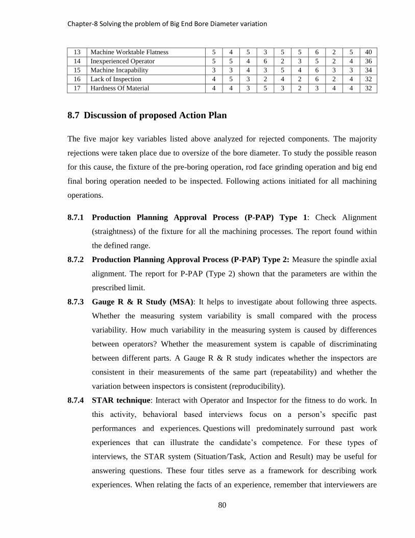
Chapter-8 Solving the problem of Big End Bore Diameter variation
80
13 Machine Worktable Flatness 5 4 5 3 5 5 6 2 5 40
14 Inexperienced Operator 5 5 4 6 2 3 5 2 4 36
15 Machine Incapability 3 3 4 3 5 4 6 3 3 34
16 Lack of Inspection 4 5 3 2 4 2 6 2 4 32
17 Hardness Of Material 4 4 3 5 3 2 3 4 4 32
8.7 Discussion of proposed Action Plan
The five major key variables listed above analyzed for rejected components. The majority
rejections were taken place due to oversize of the bore diameter. To study the possible reason
for this cause, the fixture of the pre-boring operation, rod face grinding operation and big end
final boring operation needed to be inspected. Following actions initiated for all machining
operations.
8.7.1 Production Planning Approval Process (P-PAP) Type 1: Check Alignment
(straightness) of the fixture for all the machining processes. The report found within
the defined range.
8.7.2 Production Planning Approval Process (P-PAP) Type 2: Measure the spindle axial
alignment. The report for P-PAP (Type 2) shown that the parameters are within the
prescribed limit.
8.7.3 Gauge R & R Study (MSA): It helps to investigate about following three aspects.
Whether the measuring system variability is small compared with the process
variability. How much variability in the measuring system is caused by differences
between operators? Whether the measurement system is capable of discriminating
between different parts. A Gauge R & R study indicates whether the inspectors are
consistent in their measurements of the same part (repeatability) and whether the
variation between inspectors is consistent (reproducibility).
8.7.4 STAR technique: Interact with Operator and Inspector for the fitness to do work. In
this activity, behavioral based interviews focus on a person’s specific past
performances and experiences. Questions will predominately surround past work
experiences that can illustrate the candidate’s competence. For these types of
interviews, the STAR system (Situation/Task, Action and Result) may be useful for
answering questions. These four titles serve as a framework for describing work
experiences. When relating the facts of an experience, remember that interviewers are

FMEA – Failure Mode and Effects Analysis
81
often looking for someone who’s Optimistic, Creative, a Leader and a Team player [2]
[3].
8.7.5 Patrol Inspection and Dock Inspection Report: Check the Patrol Inspection and
Dock Inspection Reports: Both the reports cross checked with the senior inspector and
found as per predefined norms. No any deviation found in the reports regarding
dimensional quality. It was mentioned in the report that the non-confirmed products
were sent to rework.
8.7.6 First Article Inspection Report (FAIR): The First Article Inspection Reports of last
months were checked. All reports found that production process met the predefined
requirements. First Piece Approval (FPA) was taken as per the inspection plans.
8.8 FMEA - Failure Mode and Effects Analysis
It is a step-by-step approach for identifying all possible failures in a design, a manufacturing
or assembly process, or a product or service. The first step is to prepare a chart of readings.
- Try to find out the trend of Non-conformance. e.g. Tool change frequency, coolant
temperature, operator, inspector, instrument, etc (To find the impact of the respective
factor on non-conformance).
- This action identified the reason for rejection in the present case. The majority of
rejections taken place due to an oval of the big end bore. The report of oval pieces
prepared for the torque applied to assemble the rods with a cap. It is found that the
rejected pieces had higher torque at the time of second assembly operation. Due to
higher torque, the possibility of an oval in big end bore increases and hence, rejection
has taken place.
A p-FMEA (Product Failure Mode and Effect Analysis) sheet for three machining processes
and two intermediate assembly processes is shown in Fig. 8.3.
From the causes enumerated in the cause and effect diagram, the failure modes and effects
analysis was performed.

Chapter-8 Solving the problem of Big End Bore Diameter variation
82
The risk priority numbers which were above 50 (as per the management decision) were
considered to be the criteria for implementing the corrective action.
It can be noticed that the highest risk priority number (RPN) is for Assembly operation.
Variation in torque value at the time of assembly of rod and cap results in bore diameter
variation and oval of the bore after dis-assembly. Hence, to mitigate these causes, a necessary
action plan was devised.
8.9 Data collection
Data collection of the key process characteristic was performed for 60 consecutive machined
components. Data to be collected and tabulated per week (one iteration per week). After each
iteration, readings are taken and recorded as represented in respective iteration tables. (Table
8.3, 8.4, 8.5, 8.6). The process monitoring chart is prepared to show process variation. The
average value of bore diameter of the group of four components is plotted on the x-axis and
respective group numbers on the y-axis.

Analysis
83
FIGURE 8.3 : Process FMEA Sheet
Op
era
tio
n N
o.
Pro
ce
ss N
am
e
Potential Failure Potential effect
Se
ve
rity
Potential Cause
Occu
rre
nce
Current Controls
De
tectio
n
Ris
k P
rio
rity
Nu
mb
er
Torque wrench settingTorque value
less/more9
Ovality of bore varies after
disassembly8 3 51
Lack of InspectionTorque value
less/more9
Ovality of bore varies after
disassembly9 3 54
Torque value in
Assembly
Torque value
less/more7 9 2 32
Lack of InspectionTorque value
less/more7 8 2 30
Ovality of bore after final
boringTaperness of bore 6
Misalignment of Axis in final
boring7
Tool set up
control in check
list
3 39
Machine IncapabilityBore diameter
variation5
measuring instruments to be
checked7
Gauge R & R
study report2 24
Big End Pre boring
oversize
Bore diameter
variation6 worn out fixture setup 8
fixture calibration
procedure report3 42
Big End Pre boring
undersizerework to be done 5
dimensional inaccuracies of
forging8
In process
Inspection Report3 39
Rod face width variation
incorrect location of
the component in
fixtures of next
operations
6dimensional inaccuracies of
forging4
Forging
Inspection Report4 40
Machine Worktable
Flatness IrregularitiesRod face taper 7
improper zero setting and
referencing of the grinding
wheel position
6
fixture calibration
procedure
document
3 39
Tool wearDimensional
variation5
improper zero setting and
referencing of the grinding
wheel position
7tool setup control
in the check list3 36
Machine IncapabilityComponent
rejection6
improper zero setting and
referencing of the grinding
wheel position
5Machine
Capability Report3 33
Lack of InspectionComponent
rejection5 Dial gauge not calibrated 6
In process
Inspection Report2 22
Big end honing oversizeImproper Fixture
Setup Process4
First Piece Approval process
not standardized5
First Piece
Approval Report
(FPA)
3 27
Big end honing undersize
incorrect location of
the component in
fixtures of next
operations
4First Piece Approval process
not standardized5
First Piece
Approval Report
(FPA)
2 18
Unskilled Operatorhoning pattern
disturbed3
Inprocess Inspection frequency
change4
Visual inspection
& IIR1 7
Inexperienced Operatorhoning pattern
disturbed4
Inprocess Inspection frequency
change4
Visual inspection
& IIR2 16
Hardness Of MaterialBore diameter
variation3
Inprocess Inspection frequency
change5
Material Test
Report2 16
Asse
mb
ly 2
19
Process Failure Modes and Effects Analysis sheet
15
Asse
mb
ly 1
In process
Inspection Report
Honning pattern not
maintained in Big End bore
Visual inspection
and bore guage
2
Ro
d F
ace
Gri
nd
ing
21
Big
En
d H
on
ing
Big
En
d P
re a
nd
Fin
al B
ori
ng
16

Chapter-8 Solving the problem of Big End Bore Diameter variation
84
8.10 Analysis
The analysis phase comprises performing the calculations for the Cp and Cpk values across
each iteration. This was followed by one-way ANOVA method of investigation to test for the
differences between the four iterations of the data sets.
8.10.1 First Iteration
The readings of the first week of 60 components are tabulated in Table 8.3. The readings are
taken after the final honing operation. The computation report indicates lower values of
process capability indices.
8.10.2 Second Iteration
In this iteration, gauge repeatability and reproducibility was performed and data were
collected as represented in Table 8.4. It is seen that there is a marginal improvement in process
capability indices. This marginal improvement is a positive sign for performed Gauge R & R.
8.10.3 Third Iteration
This iteration was performed after checking rod face width parameter. The components
selected with the lower range of variation in two parameters i.e. rod face width and taper. The
axial alignment in big end boring operation also checked and corrected as per predefined
range. The readings are taken and represented in Table 8.5. Again it shows a slight
improvement in Cp and Cpk. The process is still not capable as the values are lower. Hence
iteration is performed after other corrective action.
8.10.4 Fourth Iteration
In this iteration, data is collected after correction in torque value in both assemblies. It is
observed that the value of torque in the second assembly was not with the range. The torque
wrench for the second assembly was altered and frequency of calibration was reduced from
once in a shift to twice in a shift. The readings were taken and values of process capability
indices represented in Table 8.6 shows considerable improvement.

Analysis
85
Table 8.3 : Process Capability Report First Iteration
Sub-
Group
Readings of Big Bore Diameter xavg Range Results
1 2 3 4
1 60.842 60.840 60.839 60.834 60.839 0.008 Xavg 60.8382
2 60.838 60.839 60.838 60.833 60.837 0.006 Ravg 0.0035
3 60.834 60.833 60.838 60.835 60.835 0.005
4 60.839 60.839 60.840 60.837 60.839 0.003 USL 60.8460
5 60.837 60.837 60.838 60.839 60.838 0.002 LSL 60.8330
6 60.840 60.838 60.838 60.839 60.839 0.002
7 60.839 60.840 60.842 60.839 60.840 0.003 σ 0.00168
8 60.838 60.835 60.834 60.833 60.835 0.005
9 60.835 60.841 60.839 60.838 60.838 0.006 Cp 1.2875
10 60.842 60.841 60.839 60.840 60.841 0.003 Cpk 1.5483
11 60.839 60.839 60.837 60.839 60.839 0.002
1.0267
12 60.838 60.837 60.838 60.837 60.838 0.001
13 60.842 60.839 60.842 60.839 60.841 0.003 A2 0.73
14 60.839 60.839 60.838 60.837 60.838 0.002 D4 2.28
15 60.838 60.839 60.838 60.838 60.838 0.001
FIGURE 8.4 : First Iteration

Chapter-8 Solving the problem of Big End Bore Diameter variation
86
Table 8.4: Process Capability Study Report Second Iteration
Sub-
Group
Readings of Big Bore Diameter xavg Range Results
1 2 3 4
1 60.838 60.842 60.841 60.843 60.841 0.005 Xavg 60.8386
2 60.840 60.839 60.838 60.833 60.838 0.007 Ravg 0.0033
3 60.841 60.838 60.838 60.839 60.839 0.003
4 60.838 60.839 60.840 60.837 60.839 0.003 USL 60.8460
5 60.838 60.839 60.838 60.840 60.839 0.002 LSL 60.8330
6 60.834 60.838 60.838 60.839 60.837 0.005
7 60.838 60.837 60.838 60.839 60.838 0.002 Σ 0.00159
8 60.838 60.835 60.834 60.833 60.835 0.005
9 60.839 60.841 60.839 60.838 60.839 0.003 Cp 1.3663
10 60.839 60.841 60.839 60.840 60.840 0.002 Cpk 1.5660
11 60.842 60.839 60.837 60.839 60.839 0.005
1.1666
12 60.838 60.838 60.838 60.837 60.838 0.001
13 60.842 60.840 60.842 60.839 60.841 0.003 A2 0.73
14 60.837 60.839 60.838 60.839 60.838 0.002 D4 2.28
15 60.838 60.839 60.838 60.838 60.838 0.001
FIGURE 8.5 : Second Iteration

Analysis
87
TABLE 8.5: Process Capability Study Report Third Iteration
Sub-
Group
Readings of Big Bore Diameter xavg Range Results
1 2 3 4
1 60.834 60.838 60.838 60.839 60.837 0.005 Xavg 60.8386
2 60.839 60.840 60.839 60.837 60.839 0.003 Ravg 0.0031
3 60.842 60.841 60.842 60.843 60.842 0.002
4 60.838 60.838 60.839 60.833 60.837 0.006 USL 60.8460
5 60.837 60.838 60.837 60.839 60.838 0.002 LSL 60.8330
6 60.838 60.834 60.835 60.833 60.835 0.005
7 60.837 60.838 60.839 60.840 60.839 0.003 Σ 0.00152
8 60.840 60.838 60.838 60.839 60.839 0.002
9 60.835 60.839 60.841 60.838 60.838 0.006 Cp 1.4245
10 60.842 60.839 60.841 60.840 60.841 0.003 Cpk 1.6180
11 60.840 60.842 60.840 60.839 60.840 0.003
1.2309
12 60.839 60.838 60.839 60.839 60.839 0.001
13 60.840 60.842 60.840 60.839 60.840 0.003 A2 0.73
14 60.839 60.837 60.839 60.839 60.839 0.002 D4 2.28
15 60.838 60.838 60.838 60.837 60.838 0.001
FIGURE 8.6 : Third Iteration

Chapter-8 Solving the problem of Big End Bore Diameter variation
88
TABLE 8.6 : Process Capability Report Fourth Iteration
Sub-
Group
Readings of Big Bore Diameter xavg Range Results
1 2 3 4
1 60.838 60.838 60.838 60.842 60.839 0.004 Xavg 60.8384
2 60.837 60.838 60.839 60.838 60.838 0.002 Ravg 0.0029
3 60.838 60.838 60.838 60.842 60.839 0.004
4 60.839 60.839 60.838 60.837 60.838 0.002 USL 60.8460
5 60.837 60.837 60.838 60.838 60.838 0.001 LSL 60.8330
6 60.838 60.838 60.838 60.838 60.838 0.000
7 60.838 60.838 60.837 60.840 60.838 0.003 σ 0.00142
8 60.834 60.838 60.840 60.839 60.838 0.006
9 60.838 60.839 60.839 60.838 60.839 0.001 Cp 1.5216
10 60.838 60.839 60.837 60.838 60.838 0.002 Cpk 1.7908
11 60.840 60.842 60.843 60.838 60.841 0.005
1.2524
12 60.839 60.838 60.833 60.834 60.836 0.006
13 60.840 60.842 60.839 60.838 60.840 0.004 A2 0.73
14 60.840 60.837 60.839 60.839 60.839 0.003 D4 2.28
15 60.838 60.838 60.838 60.837 60.838 0.001
FIGURE 8.7 : Fourth Iteration
8.11 Process capability study report compilation
This phase is related to select those product performance characteristics which must be
improved to achieve the goal. In the present case, few aspects need to have attention as far as
quality is concerned. The causes and reasons matrix is drawn and results are entered and the

Implemented action plan
89
improvement actions that are to be taken are listed. The values of process capability indices
are stated to indicate the impact of implemented actions.
TABLE 8.7 : Compiled Process Capability Study Reports
Cause Reason Actions to be implemented
Process Capability
Indices
Cp Cpk
More rework after
final honing
operation
Operator tendency to
work on lower side
Instructed operator to do honing
to mean value of bore diameter. 1.2875
1.5483
1.0267
Bore diameter
variation
Bore Gauge variation
in reading
Gauge R & R study to be
conducted. 1.3663
1.5660
1.1666
Rod face width
variation
Fixture setup not
done properly The fixture to be set properly. 1.4245
1.6180
1.2309
Torque value of nut
and bolt assembly
varies
Torque wrench not
checked regularly
Torque wrench checking
frequency decided. 1.5216
1.7902
1.2524
8.12 Implemented action plan
The value of torque at the time of the second assembly of connecting rod should be
maintained in the pre-defined range. The use of precise torque wrench is proposed to have
better accuracy in an assembly operation. It is also proposed to do the calibration of the torque
wrench regularly. Further, it is also decided to check a sample of a batch for torque at the time
of the second assembly of rod and cap. This reduced the possibility of rejection in big end
bore diameter variation up to a considerable extent. This phase assures that the implemented
action will sustain and it is incorporated into the system.
8.13 Conclusion
Assembly of the connecting rod during manufacturing operations needs to be performed in the
pre-defined range. When rod and cap are assembled, the value of torque applied to bolts
makes the great impact over the dimensional quality of connecting rod. The quality of
subsequent operations of connecting rod depends on the tightness of the rod and cap. The
higher value of torque results in ovality of big end bore. The lower value of torque may cause
vibration and parting line misalignment and ultimately bend and twist of the connecting rod.

Chapter-8 Solving the problem of Big End Bore Diameter variation
90
The objective of introducing the Six Sigma – DMAIC methodology to the concern by
applying it to the most chronic problem faced by the company was successfully achieved. The
implementation of it resulted in understanding the problem from all aspects, qualitatively as
well as quantitatively, and laying out the improvements through effective analysis of the roots
of the problem.

Performance Excellence
91
CHAPTER – 9
Computation of Performance Excellence, Conclusion
and Future Scope
9.1 Performance Excellence
Excellence means a talent or quality which is good and so surpasses ordinary standards.
Excellence is a quality that people really appreciate because it's so difficult to discover. It is
also used as a standard of performance. The meaning of excellence is to improve the existing
one. Performance excellence means to improve the existing situation.
According to NIST, Performance excellence refers to an integrated approach to organizational
performance management that result in, delivery of ever-improving value to customers and
stakeholders, contributing to organizational sustainability, Improvement of overall
organizational effectiveness and capabilities and oorganizational and personal learning [60].
It is difficult to statistically justify actual impact of any alteration or modification made on the
shop floor. Many factors should be considered before and after modification employed. The
method to compute performance excellence includes some statistical parameters like rework
quantity, rejection quantity, inventory, customer complaints, scrape quantity and production
quantity. The reduction in these parameters illustrates the implementation of performance
excellence in connecting rod manufacturing industries.

CHAPTER – 9 Computation of Performance Excellence, Conclusion and Future Scope
92
9.2 Data analysis
Statistical Process Control report prepared for critical parameters of connecting rod represent
the improvement in terms of quality. The Tables 9.1 to 9.7 represent the improvement in
performance of connecting rod manufacturing processes.
The graph represents the improvement in values of process capability indices. The higher
value of these indices represents more stability of the process.

Performance Excellence
93
TABLE 9.1 : Big End Bore Diameter
PART NAME: Con Rod INSTRUMENT USED: Air Guage
PART NO.: LEAST COUNT: 0.001 mm
CUSTOMER NAME: M/s. Simpson M/C NO.: 07-08iXi
OPERATION NAME: Honning MACHINE NAME: Manisa
PARAMETER: Big End Diameter OPERATOR NAME: Birju Patel
SUB-
GROUP 1 2 3 4 X R
1 60.842 60.840 60.839 60.838 60.840 0.004 X 60.8388 CONTROL LIMITS: INTERPRETATION
2 60.838 60.839 60.838 60.839 60.839 0.001 R 0.0022 UCLX 60.8404 Cp<1.00
3 60.839 60.837 60.838 60.839 60.838 0.002 UTL 60.8460 LCLX 60.8372 1. Process is not capable
4 60.839 60.839 60.840 60.837 60.839 0.003 LTL 60.8330 UCLR 0.0050 - try to shift the job to
5 60.837 60.837 60.838 60.839 60.838 0.002 0.00107 LCLR 0.0000 another process with
6 60.840 60.838 60.838 60.839 60.839 0.002 Cp 2.0288 A2 D4 adequate capability
7 60.839 60.840 60.842 60.839 60.840 0.003 Cpk 2.2369 0.73 2.28 -try to improve capability
8 60.838 60.839 60.838 60.838 60.838 0.001 1.8207 Cp=1.00
9 60.838 60.841 60.839 60.838 60.839 0.003 1. Process is just capable
10 60.842 60.841 60.839 60.840 60.841 0.003 Comments (If any): Cp>1.00
11 60.839 60.839 60.837 60.839 60.839 0.002 1. Process is quite capable
12 60.838 60.837 60.838 60.837 60.838 0.001 Cp>1.67
13 60.842 60.839 60.842 60.839 60.841 0.003 1. Process is capable
14 60.839 60.839 60.838 60.837 60.838 0.002 Cpk<1.67
15 60.838 60.839 60.838 60.838 60.838 0.001 1. Machine setting required
JAN FEB MARCH APRIL MAY JUNE JULY AUG SEP OCT NOV DEC
Cp 1.71 1.91 2.15 1.91 2.00 2.03
Cpk 1.51 1.65 1.90 1.71 1.90 1.82
READINGS
RESULTS
0.00
0.50
1.00
1.50
2.00
2.50
JAN FEB MARCH APRIL MAY JUNE JULY AUG SEP OCT NOV DEC
Cp
/Cp
k
Month
Cp/Cpk Continuous Monitoring
Cp
Cpk

CHAPTER – 9 Computation of Performance Excellence, Conclusion and Future Scope
94
TABLE 9.2 : Small End Boring (Parent bore-without bush)
PART NAME: Con Rod INSTRUMENT USED: Air Guage
CUSTOMER NAME: LEAST COUNT: 0.001 mm
CUSTOMER NAME: M/s. Simpson M/C NO.: G2709ix
OPERATION NAME: Boring MACHINE NAME: Gehring
PARAMETER: Bore Diameter OPERATOR NAME: Kalu Mal
SUB-
GROUP 1 2 3 4 X R
1 34.945 34.937 34.941 34.940 34.941 0.008 X 34.9395 CONTROL LIMITS: INTERPRETATION
2 34.937 34.945 34.935 34.938 34.939 0.010 R 0.0061 UCLX 34.9439 Cp<1.00
3 34.940 34.937 34.937 34.945 34.940 0.008 UTL 34.9560 LCLX 34.9350 1. Process is not capable
4 34.937 34.941 34.940 34.937 34.939 0.004 LTL 34.9200 UCLR 0.0140 - try to shift the job to
5 34.937 34.937 34.938 34.941 34.938 0.004 0.00298 LCLR 0.0000 another process with
6 34.937 34.937 34.945 34.940 34.940 0.008 Cp 2.0152 A2 D4 adequate capability
7 34.935 34.937 34.937 34.941 34.938 0.006 Cpk 1.8510 0.73 2.28 -try to improve capability
8 34.937 34.935 34.940 34.940 34.938 0.005 2.1794 Cp=1.00
9 34.940 34.937 34.937 34.940 34.939 0.003 1. Process is just capable
10 34.938 34.940 34.937 34.937 34.938 0.003 Comments (If any): Cp>1.00
11 34.945 34.938 34.937 34.945 34.938 0.008 1. Process is quite capable
12 34.937 34.940 34.935 34.937 34.941 0.005 Cp>1.67
13 34.941 34.935 34.937 34.941 34.942 0.006 1. Process is capable
14 34.945 34.940 34.937 34.937 34.945 0.008 Cpk<1.67
15 34.937 34.941 34.935 34.935 34.938 0.006 1. Machine setting required
JAN FEB MARCH APRIL MAY JUNE JULY AUG SEP OCT NOV DEC
Cp 1.87 1.97 2.03 2.18 2.00 2.01
Cpk 1.70 1.82 1.86 2.00 1.80 1.85
READINGS
RESULTS
0.00
0.50
1.00
1.50
2.00
2.50
3.00
JAN FEB MARCH APRIL MAY JUNE JULY AUG SEP OCT NOV DEC
Cp
/Cp
k
Month
Cp/Cpk Continuous Monitoring
Cp
Cpk

Performance Excellence
95
TABLE 9.3 : Bolt Hole Drilling
PART NAME: Con Rod INSTRUMENT USED: Air Guage
PART NO.: LEAST COUNT: 0.001 mm
CUSTOMER NAME:M/s. Simpson M/C NO.: BHxddi
OPERATION NAME: Bolt Hole Drilling MACHINE NAME: Aurum Multy Spindle Drilling Machine
PARAMETER: Bolt Hole Diameter OPERATOR NAME: Manoj pai
SUB-
GROUP 1 2 3 4 X R
1 11.138 11.135 11.130 11.142 11.136 0.012 X 11.1327 CONTROL LIMITS: INTERPRETATION
2 11.131 11.134 11.131 11.130 11.132 0.004 R 0.0067 UCLX 11.1376 Cp<1.00
3 11.130 11.130 11.135 11.131 11.132 0.005 UTL 11.1500 LCLX 11.1278 1. Process is not capable
4 11.131 11.131 11.138 11.135 11.134 0.007 LTL 11.1000 UCLR 0.0154 -try to shift the job to
5 11.138 11.126 11.135 11.131 11.133 0.012 0.00327 LCLR 0.0000 another process with
6 11.131 11.135 11.134 11.138 11.135 0.007 Cp 2.5495 A2 D4 adequate capability
7 11.131 11.135 11.138 11.142 11.137 0.011 Cpk 1.7626 0.73 2.28 -try to improve capability
8 11.126 11.131 11.131 11.131 11.130 0.005 3.3365 Cp=1.00
9 11.142 11.130 11.130 11.135 11.134 0.012 1. Process is just capable
10 11.130 11.131 11.131 11.131 11.131 0.001 Comments (If any): Cp>1.00
11 11.131 11.131 11.138 11.130 11.133 0.008 1. Process is quite capable
12 11.135 11.135 11.131 11.131 11.133 0.004 Cp>1.67
13 11.131 11.134 11.131 11.126 11.131 0.008 1. Process is capable
14 11.134 11.131 11.131 11.135 11.133 0.004 Cpk<1.67
15 11.131 11.130 11.131 11.131 11.131 0.001 1. Machine setting required
JAN FEB MARCH APRIL MAY JUNE JULY AUG SEP OCT NOV DEC
Cp 2.14 2.36 2.52 2.57 2.40 2.54
Cpk 1.51 1.66 1.75 1.80 1.90 1.76
READINGS
RESULTS
0.00
0.50
1.00
1.50
2.00
2.50
3.00
JAN FEB MARCH APRIL MAY JUNE JULY AUG SEP OCT NOV DEC
Cp
/Cp
k
Month
CP/Cpk Continuous Monitoring
Cp
Cpk

CHAPTER – 9 Computation of Performance Excellence, Conclusion and Future Scope
96
TABLE 9.4 : Center Distance
PART NAME: Con Rod INSTRUMENT USED: Task Special Purpose Guage
PART NO.: LEAST COUNT: 0.001 mm
CUSTOMER NAME: M/s. Simpson M/C NO.: 17-08-00
OPERATION NAME: Small End Bush Boring MACHINE NAME: Profitech
PARAMETER: Center Distance OPERATOR NAME: Rajan Pal
SUB-
GROUP 1 2 3 4 X R
1 223.840 223.847 223.841 223.838 223.842 0.009 X 223.8414 CONTROL LIMITS: INTERPRETATION
2 223.839 223.845 223.839 223.847 223.843 0.008 R 0.0087 UCLX 223.8478 Cp<1.00
3 223.838 223.838 223.847 223.841 223.841 0.009 UTL 223.8630 LCLX 223.8351 1. Process is not capable
4 223.847 223.847 223.836 223.839 223.842 0.011 LTL 223.8120 UCLR 0.0199 -try to shift the job to
5 223.840 223.847 223.845 223.847 223.845 0.007 0.00424 LCLR 0.0000 another process with
6 223.847 223.845 223.838 223.838 223.842 0.009 Cp 2.0050 A2 D4 adequate capability
7 223.841 223.838 223.840 223.845 223.841 0.007 Cpk 1.6957 0.73 2.28 -try to improve capability
8 223.841 223.847 223.839 223.838 223.841 0.009 2.3142 Cp=1.00
9 223.839 223.839 223.838 223.844 223.840 0.006 1. Process is just capable
10 223.847 223.847 223.847 223.838 223.845 0.009 Comments (If any): Cp>1.00
11 223.836 223.836 223.840 223.842 223.839 0.006 1. Process is quite capable
12 223.845 223.845 223.847 223.839 223.844 0.008 Cp>1.67
13 223.838 223.838 223.841 223.837 223.839 0.004 1. Process is capable
14 223.838 223.838 223.830 223.847 223.838 0.017 Cpk<1.67
15 223.847 223.836 223.847 223.835 223.841 0.012 1. Machine setting required
JAN FEB MARCH APRIL MAY JUNE JULY AUG SEP OCT NOV DEC
Cp 1.99 1.96 2.05 1.90 2.01 2.11
Cpk 1.60 1.62 1.65 1.63 1.72 1.78
READINGS
RESULTS
0.00
0.50
1.00
1.50
2.00
2.50
JAN FEB MARCH APRIL MAY JUNE JULY AUG SEP OCT NOV DEC
Cp
/Cp
k
Month
Cp/Cpk Continuous Monitoring
Cp
Cpk

Performance Excellence
97
TABLE 9.5 : Bend (Axial Mis-alignment)
PART NAME: Con Rod INSTRUMENT USED: V Block, Pins, Height Gauge
PART NO.: LEAST COUNT: 0.001 mm
CUSTOMER NAME: M/s. Simpson M/C NO.: xn99d
OPERATION NAME: Small End Bush Boring MACHINE NAME: Profitech
PARAMETER: Bend OPERATOR NAME: Nayan Sahu
SUB-
GROUP 1 2 3 4 X R
1 0.003 -0.001 0.004 0.003 0.002 0.005 X 0.0008 CONTROL LIMITS: INTERPRETATION
2 -0.004 -0.003 -0.003 -0.003 -0.003 0.001 R 0.0037 UCLX 0.0035 Cp<1.00
3 0.003 0.002 0.003 0.004 0.003 0.002 UTL 0.0100 LCLX -0.0020 1. Process is not capable
4 -0.001 0.001 -0.003 -0.004 -0.002 0.005 LTL 0.0000 UCLR 0.0085 -try to shift the job to
5 0.004 0.005 0.002 0.001 0.003 0.004 0.00181 LCLR 0.0000 another process with
6 0.004 0.003 0.005 0.003 0.004 0.002 Cp 0.9196 A2 D4 adequate capability
7 -0.004 0.003 0.003 0.002 0.001 0.007 Cpk 1.6983 0.73 2.28 -try to improve capability
8 -0.004 -0.003 -0.004 -0.003 -0.004 0.001 1.6700 Cp=1.00
9 0.003 0.005 0.003 0.004 0.004 0.002 1. Process is just capable
10 0.002 0.003 0.004 0.003 0.003 0.002 Comments (If any): Cp>1.00
11 -0.004 -0.001 -0.004 -0.006 -0.004 0.005 1. Process is quite capable
12 -0.001 0.003 0.001 0.001 0.001 0.004 Cp>1.67
13 0.003 0.003 -0.001 0.005 0.003 0.006 1. Process is capable
14 -0.001 0.002 0.003 0.002 0.002 0.004 Cpk<1.67
15 -0.003 0.002 -0.004 0.001 -0.001 0.006 1. Machine setting required
JAN FEB MARCH APRIL MAY JUNE JULY AUG SEP OCT NOV DEC
Cp 1.70 1.70 1.68 1.70 1.71 1.73
Cpk 1.600 1.630 1.650 1.660 1.690 1.670
RESULTS
READINGS
1.50
1.55
1.60
1.65
1.70
1.75
JAN FEB MARCH APRIL MAY JUNE JULY AUG SEP OCT NOV DEC
Cp
/Cp
k
Month
Cp/Cpk continuous Monitoring
Cp

CHAPTER – 9 Computation of Performance Excellence, Conclusion and Future Scope
98
TABLE 9.6 : Small End Diameter (After Bush Boring)
PART NAME: Con Rod INSTRUMENT USED: Air Guage
PART NO.: LEAST COUNT: 0.001 mm
CUSTOMER NAME: M/s. Simpson M/C NO.: 17-08-00
OPERATION NAME: Small End Bush Boring MACHINE NAME: Profitech
PARAMETER: Bush Diameter OPERATOR NAME: Nayan Sahu
SUB-
GROUP 1 2 3 4 X R
1 31.773 31.772 31.773 31.776 31.774 0.004 X 31.7765 CONTROL LIMITS: INTERPRETATION
2 31.774 31.773 31.776 31.773 31.774 0.003 R 0.0045 UCLX 31.7798 Cp<1.00
3 31.773 31.774 31.779 31.774 31.780 0.006 UTL 31.7880 LCLX 31.7733 1. Process is not capable
4 31.774 31.771 31.773 31.772 31.773 0.003 LTL 31.7630 UCLR 0.0102 -try to shift the job to
5 31.779 31.771 31.773 31.773 31.780 0.008 0.00217 LCLR 0.0000 another process with
6 31.776 31.775 31.776 31.776 31.776 0.001 Cp 1.9216 A2 D4 adequate capability
7 31.779 31.779 31.776 31.775 31.780 0.004 Cpk 1.7653 0.73 2.28 -try to improve capability
8 31.779 31.773 31.773 31.773 31.775 0.006 2.0779 Cp=1.00
9 31.773 31.779 31.773 31.773 31.775 0.006 1. Process is just capable
10 31.776 31.773 31.774 31.772 31.780 0.004 Comments (If any): Cp>1.00
11 31.779 31.771 31.773 31.773 31.774 0.008 1. Process is quite capable
12 31.773 31.776 31.776 31.772 31.780 0.004 Cp>1.67
13 31.776 31.775 31.779 31.771 31.775 0.008 1. Process is capable
14 31.776 31.776 31.776 31.776 31.780 0.000 Cpk<1.67
15 31.773 31.774 31.773 31.775 31.774 0.002 1. Machine setting required
JAN FEB MARCH APRIL MAY JUNE JULY AUG SEP OCT NOV DEC
Cp 1.78 1.92 1.95 2.01 1.78 1.92
Cpk 1.61 1.71 1.75 1.79 1.70 1.76
READINGS
RESULTS
0.00
0.50
1.00
1.50
2.00
2.50
JAN FEB MARCH APRIL MAY JUNE JULY AUG SEP OCT NOV DEC
Cp
/cp
k
Month
Cp/Cpk Continuous Monitoring
Cp
Cpk

Performance Excellence
99
TABLE 9.7 : Twist (Axial Mis-alignment)
PART NAME: Con Rod INSTRUMENT USED: V Block, Pins, Height Gauge
PART NO.: LEAST COUNT: 0.001 mm
CUSTOMER NAME: M/s. Simpson M/C NO.: bkXn
OPERATION NAME: Small End Bush Boring MACHINE NAME: Profitech
PARAMETER: Twist OPERATOR NAME: Nayan Sahu
SUB-
GROUP 1 2 3 4 X R
1 -0.002 -0.003 0.001 0.001 -0.001 0.004 X 0.0013 CONTROL LIMITS: INTERPRETATION
2 -0.003 -0.002 -0.002 -0.002 -0.002 0.001 R 0.0023 UCLX 0.0030 Cp<1.00
3 0.003 0.002 0.004 0.003 0.003 0.002 UTL 0.0100 LCLX -0.0004 1. Process is not capable
4 0.002 0.005 0.003 0.003 0.003 0.003 LTL 0.0000 UCLR 0.0053 - try to shift the job to
5 0.002 0.003 0.002 0.002 0.002 0.001 0.00113 LCLR 0.0000 another process with
6 -0.001 -0.002 0.002 0.002 0.000 0.004 Cp 1.7000 A2 D4 adequate capability
7 0.002 0.003 0.003 0.002 0.003 0.001 Cpk 1.6700 0.73 2.28 -try to improve capability
8 0.005 0.002 0.003 0.003 0.003 0.003 1.6900 Cp=1.00
9 -0.003 -0.002 -0.002 -0.002 -0.002 0.001 1. Process is just capable
10 0.002 0.005 0.002 0.002 0.003 0.003 Comments (If any): Cp>1.00
11 0.005 0.005 0.005 0.005 0.005 0.000 1. Process is quite capable
12 0.001 0.003 0.002 0.003 0.002 0.002 Cp>1.67
13 -0.003 0.001 -0.004 0.002 -0.001 0.006 1. Process is capable
14 0.002 0.002 0.002 0.002 0.002 0.000 Cpk<1.67
15 -0.003 0.000 -0.002 0.001 -0.001 0.004 1. Machine setting required
JAN FEB MARCH APRIL MAY JUNE JULY AUG SEP OCT NOV DEC
Cp 1.77 1.90 1.92 1.98 1.89 1.99
Cpk 1.6 1.6 1.7 1.7 1.7 1.7
READINGS
RESULTS
0.00
0.50
1.00
1.50
2.00
2.50
JAN FEB MARCH APRIL MAY JUNE JULY AUG SEP OCT NOV DEC
Cp
/Cp
k
Month
Cp/Cpk Continuous Monitoring Cp
Cpk

CHAPTER – 9 Computation of Performance Excellence, Conclusion and Future Scope
100
It can be concluded from Tables 9.1 to 9.7 that the processes are under statistical control, as
the values of process capability indices are higher. It can also be concluded that there is an
improvement in the values of process capability indices in each case.
The data represented in Table 9.8 shows the rework quantity year wise and parameter wise.
Table 9.9 shows the rejection quantity year wise. The graph is shown in Fig. 9.1 and Fig. 9.2
represents the reduction in rework and rejection quantity year wise. The quantity of production
is shown in Fig. 9.3.
The reduction in rework and rejection ultimately results in the reduction in customer
complaints and hence customer satisfaction. The ultimate aim of present work is to enhance
the customer satisfaction by employing various quality improvement techniques.

Performance Excellence
101
TABLE 9.8 : Rework Quantity year wise
Sr.
No. Parameters
Actual Production Quantity Q (year wise)
2012-13 2013-2014 2014-15 2015-16
Q = 65184 Q = 71349 Q = 75723 Q = 79803
Rework
pcs %
Rework
pcs %
Rework
pcs %
Rework
pcs %
1 Big End bore
diameter 890 1.37 1105 1.55 987 1.30 1011 1.27
2 Small End bore
diameter 824 1.26 998 1.40 787 1.04 976 1.22
3 Center Distance
(C.D.) 909 1.39 802 1.12 839 1.11 56 0.07
4 Bend 891 1.37 782 1.10 445 0.59 40 0.05
5 Twist 793 1.22 292 0.41 432 0.57 28 0.04
6 End Float more/less 34 0.05 43 0.06 23 0.03 42 0.05
7 Big end bore width 45 0.07 54 0.08 43 0.06 45 0.06
8 Rib diameter
variation 193 0.30 64 0.09 22 0.03 64 0.08
9 Honing pattern in big
end bore 765 1.17 654 0.92 43 0.06 23 0.03
10 Big End Bore Oval 821 1.26 665 0.93 342 0.45 65 0.08
11 Surface Finish in Big
End Bore 678 1.04 564 0.79 42 0.06 43 0.05
12 Surface Finish in
Small End Bore 192 0.29 43 0.06 556 0.73 28 0.04
13 Big End bore Taper 345 0.53 543 0.76 65 0.09 78 0.10
14 Small End bore
Taper 392 0.60 453 0.63 433 0.57 54 0.07
15 Oil Hole Diameter in
Small End 232 0.36 122 0.17 344 0.45 65 0.08
16 Cap Face Taper 324 0.50 329 0.46 343 0.45 34 0.04
17 Cap Face Surface
Finish 45 0.07 53 0.07 2 0.00 5 0.01
18 Rod Face Taper 49 0.08 45 0.06 34 0.04 8 0.01
Cont…

CHAPTER – 9 Computation of Performance Excellence, Conclusion and Future Scope
102
TABLE 9.8 : Rework Quantity year wise
Sr.
No.
Rejection
Parameters
Actual Production Quantity Q (year wise)
2012-13 2013-2014 2014-15 2015-16
Q = 65184 Q = 71349 Q = 75723 Q = 79803
Rework
pcs %
Rework
pcs %
Rework
pcs %
Rework
pcs %
19 Rod Face Surface
Finish 34 0.05 98 0.14 34 0.04 76 0.10
20
Squareness of Small
End face w. r. t. Big
End Bore
78 0.12 45 0.06 56 0.07 75 0.09
21 Big End Chamfer
Diameter 29 0.04 85 0.12 6 0.01 78 0.10
22 Big End Chamfer
angle 273 0.42 86 0.12 65 0.09 79 0.10
23 Parting face Finish
Rod+Cap 54 0.08 451 0.63 56 0.07 54 0.07
24 Cap rib dimension 46 0.07 676 0.95 36 0.05 5 0.01
25 Rod spot face
dimension 340 0.52 43 0.06 78 0.10 56 0.07
26 Rod Spot face
surface finish 89 0.14 54 0.08 67 0.09 65 0.08
27 Bolt Hole Center
Distance 53 0.08 45 0.06 5 0.01 4 0.01
28 Bolt Hole Diameter 98 0.15 75 0.11 34 0.04 29 0.04
29 Notch Length Rod &
Cap 45 0.07 65 0.09 4 0.01 3 0.00
30 Notch Depth Rod &
Cap 36 0.06 43 0.06 34 0.04 5 0.01
31 Notch Width Rod &
Cap 32 0.05 67 0.09 52 0.07 2 0.00
32 Magnetism 25 0.04 34 0.05 43 0.06 30 0.04
33 Visual Inspection 0 0.00 0 0.00 0 0.00 0 0.00
34 Packing 0 0.00 0 0.00 0 0.00 0 0.00
35 Others 60 0.09 56 0.08 76 0.10 50 0.06
Total Rework 9714 14.90 9534 13.36 6428 8.49 3276 4.11

Performance Excellence
103
TABLE 9.9 : Rejection Quantity year wise
Sr.
No.
Rejection
Parameters
Actual Production Quantity Q (year wise)
2012-13 2013-2014 2014-15 2015-16
Q = 65184 Q = 71349 Q = 75723 Q = 79803
Rejection
pcs %
Rejection
pcs %
Rejection
pcs %
Rejection
pcs %
1 Big End bore
diameter 95 0.15 87 0.12 78 0.10 65 0.08
2 Small End bore
diameter 101 0.15 98 0.14 65 0.09 57 0.07
3 Center Distance
(C.D.) 36 0.06 53 0.07 52 0.07 45 0.06
4 Bend 323 0.50 36 0.05 34 0.04 30 0.04
5 Twist 234 0.36 45 0.06 65 0.09 59 0.07
6 End Float
more/less 753 1.16 44 0.06 23 0.03 20 0.03
7 Big end bore
width 36 0.06 54 0.08 12 0.02 65 0.08
8 Rib diameter
variation 64 0.10 34 0.05 43 0.06 3 0.00
9 Honing pattern in
big end bore 56 0.09 56 0.08 23 0.03 3 0.00
10 Big End Bore
Oval 22 0.03 243 0.34 67 0.09 45 0.06
11 Surface Finish in
Big End Bore 21 0.03 65 0.09 87 0.11 53 0.07
12 Surface Finish in
Small End Bore 4 0.01 57 0.08 56 0.07 39 0.05
13 Big End bore
Taper 65 0.10 56 0.08 36 0.05 22 0.03
14 Small End bore
Taper 6 0.01 43 0.06 75 0.10 47 0.06
15
Oil Hole
Diameter in
Small End
0 0.00 67 0.09 87 0.11 43 0.05
16 Cap Face Taper 0 0.00 87 0.12 45 0.06 43 0.05
17 Cap Face Surface
Finish 9 0.01 97 0.14 96 0.13 89 0.11
18 Rod Face Taper 0 0.00 54 0.08 23 0.03 19 0.02
Cont…

CHAPTER – 9 Computation of Performance Excellence, Conclusion and Future Scope
104
TABLE 9.9 : Rejection Quantity year wise
Sr.
No.
Rejection
Parameters
Actual Production Quantity Q (year wise)
2012-13 2013-2014 2014-15 2015-16
Q = 65184 Q = 71349 Q = 75723 Q = 79803
Rejection
pcs %
Rejection
pcs %
Rejection
pcs %
Rejection
pcs %
19 Rod Face Surface
Finish 3 0.00 23 0.03 54 0.07 36 0.05
20
Squareness of
Small End face
w.r.t. Big End
Bore
4 0.01 9 0.01 3 0.00 3 0.00
21 Big End Chamfer
Diameter 5 0.01 8 0.01 7 0.01 4 0.01
22 Big End Chamfer
angle 3 0.00 7 0.01 4 0.01 5 0.01
23 Parting face
Finish Rod+Cap 2 0.00 8 0.01 3 0.00 2 0.00
24 Cap rib
dimension 6 0.01 9 0.01 5 0.01 1 0.00
25 Rod spot face
dimension 7 0.01 5 0.01 6 0.01 2 0.00
26 Rod Spot face
surface finish 5 0.01 4 0.01 7 0.01 4 0.01
27 Bolt Hole Center
Distance 4 0.01 3 0.00 2 0.00 6 0.01
28 Bolt Hole
Diameter 5 0.01 5 0.01 8 0.01 6 0.01
29 Notch Length
Rod & Cap 3 0.00 0 0.00 2 0.00 3 0.00
30 Notch Depth Rod
& Cap 7 0.01 0 0.00 1 0.00 0 0.00
31 Notch Width Rod
& Cap 8 0.01 2 0.00 2 0.00 0 0.00
32 Magnetism 0 0.00 0 0.00 0 0.00 0 0.00
33 Visual Inspection 0 0.00 0 0.00 0 0.00 0 0.00
34 Packing 0 0.00 0 0.00 0 0.00 0 0.00
35 Others 9 0.01 28 0.04 40 0.05 5 0.01
Total Rejection 1896 2.91 1387 1.94 1111 1.47 824 1.03

Performance Excellence
105
FIGURE 9.1 : Rework % year wise
FIGURE 9.2 : Rejection % year wise
FIGURE 9.3 : Production per year

CHAPTER – 9 Computation of Performance Excellence, Conclusion and Future Scope
106
TABLE 9.10 : Parameter wise Total Rework
( From 1st April, 2012 to 31
st March, 2016)
Sr. Parameter Rework
Qnty. %
Sr. Parameter Rework
Qnty. %
1 Big End bore
diameter 3993 1.37 19
Rod Spot face
surface finish 275 0.09
2 Small End bore
diameter 3585 1.23 20
Squareness of Small
End face w.r.t. Big
End Bore
254 0.09
3 Center Distance
(C.D.) 2606 0.89 21
Rod Face Surface
Finish 242 0.08
4 Bend 2158 0.74 22 Others 242 0.08
5 Big End Bore
Oval 1893 0.65 23 Bolt Hole Diameter 236 0.08
6 Twist 1545 0.53 24 Big End Chamfer
Diameter 198 0.07
7 Honing pattern
in big end bore 1485 0.51 25 Big end bore width 187 0.06
8 Small End bore
Taper 1332 0.46 26
Notch Width Rod &
Cap 153 0.05
9 Surface Finish in
Big End Bore 1327 0.45 27 End Float more/less 142 0.05
10 Big End bore
Taper 1031 0.35 28 Rod Face Taper 136 0.05
11 Cap Face Taper 1030 0.35 29 Magnetism 132 0.05
12 Surface Finish in
Small End Bore 819 0.28 30
Notch Depth Rod &
Cap 118 0.04
13
Oil Hole
Diameter in
Small End
763 0.26 31 Notch Length Rod
& Cap 117 0.04
14 Cap rib
dimension 763 0.26 32
Bolt Hole Center
Distance 107 0.04
15 Parting face
Finish Rod+Cap 615 0.21 33
Cap Face Surface
Finish 105 0.04
16 Rod spot face
dimension 517 0.18 34 Visual Inspection 0 0.00
17 Big End
Chamfer angle 503 0.17 35 Packing 0 0.00
18 Rib diameter
variation 343 0.12 Total 28952 9.91

Objectives achieved
107
TABLE 9.11 : Parameter wise Total Rejection
( From 1st April 2012 to 31
st March 2016)
Sr. Parameter Rejection
Qnty. %
Sr. Parameter Rejection
Qnty. %
1 End Float
more/less 840 0.29 19 Rod Face Taper 96 0.03
2 Bend 423 0.14 20 Others 82 0.03
3 Twist 403 0.14 21 Big End Chamfer
Diameter 24 0.01
4 Big End Bore
Oval 377 0.13 22 Bolt Hole Diameter 24 0.01
5 Big End bore
diameter 325 0.11 23 Cap rib dimension 21 0.01
6 Small End bore
diameter 321 0.11 24
Rod spot face
dimension 20 0.01
7 Cap Face
Surface Finish 291 0.10 25
Rod Spot face surface
finish 20 0.01
8 Surface Finish in
Big End Bore 226 0.08 26
Squareness of Small
End face w. r. t. Big
End Bore
19 0.01
9
Oil Hole
Diameter in
Small End
197 0.07 27 Big End Chamfer
angle 19 0.01
10 Center Distance
(C.D.) 186 0.06 28
Parting face Finish
Rod+Cap 15 0.01
11 Big End bore
Taper 179 0.06 29
Bolt Hole Center
Distance 15 0.01
12 Cap Face Taper 175 0.06 30 Notch Width Rod &
Cap 12 0.00
13 Small End bore
Taper 171 0.06 31
Notch Length Rod &
Cap 8 0.00
14 Big end bore
width 167 0.06 32
Notch Depth Rod &
Cap 8 0.00
15 Surface Finish in
Small End Bore 156 0.05 33 Magnetism 0 0.00
16 Rib diameter
variation 144 0.05 34 Visual Inspection 0 0.00
17 Honing pattern
in big end bore 138 0.05 35 Packing 0 0.00
18 Rod Face
Surface Finish 116 0.04 Total 5218 1.79

CHAPTER – 9 Computation of Performance Excellence, Conclusion and Future Scope
108
9.3 Objectives Achieved
The key contributions of the thesis can be summarized by following.
1. The improvement potentials are identified in manufacturing processes of the
connecting rod.
2. The improvement in Customer satisfaction attained by reducing the reduction in
rework and rejection every year.
3. Various shop floor issues related to Connecting Rod manufacturing operations are
solved using various problem-solving techniques.
4. Performance Excellence is achieved as the percentage of rejection and rework reduces
continuously as shown in Fig. 9.1 and 9.2 even there is the rise in production shown in
Fig. 9.3.
9.4 Conclusion
In Present work, various problems related to quality are solved using TMS (Tailor-Made
solution). The generalization of such TMS becomes little beat challenging as it may not give a
better result for the same kind of other problem. The generalized approach discussed in
present work would be highly significant for the people involved in connecting rod
manufacturing to enhance their existing performance.
The present work highlights the employability of various quality improvement aspects like
Cause and Effect diagram, Brainstorming, Failure Mode and Effects Analysis, Kaizen, Six
Sigma, etc. The corrective actions proposed with the help of these aspects are implemented in
a structured way within the constraints. Hence, Performance Excellence in connecting rod
manufacturing industries is implemented.

Objectives achieved
109
The first case covered Overall Equipment Effectiveness (OEE) in connecting rod
manufacturing processes is prepared. The OEE sheet enables companies to attain a rapid
assessment of their operations performance. It highlights the gray area of the shop floor. The
OEE sheet discussed is a dominant tool to evaluate the current state and to plan the future state
of enterprise operations. This sheet is employed in a connecting rod manufacturing industries
to provide decision-makers with adequate input to identify improvement objectives and review
the ongoing operations strategy.
The second case is conducted for bush boring operation. After a bush boring operation, in
Small End of connecting rod, pillar drill is used to eliminate dent marks and burrs, as a
replacement for manual de-burring operation. It reduces manual work with better concentricity
of small end and improves the quality of product up to a considerable extent. Assembly of
gudgeon pin in the small end of connecting rod becomes easier as compared to the previous
method due to chamfered end.
The third case covered the discussion and solution of a technical problem identified from
customer complaint redressal form . The study examined one of the shop floors long-lasting
quality issues to maintain the End Float in a connecting rod during the manufacturing process.
The corrective actions for the problem are discussed and implemented which improves the
customer satisfaction and reduces the rejection quantity. The fixture of one of the
manufacturing operations is to be redesigned and altered.
The fourth case covered the statistical control of customer defined critical parameter i.e. axial
alignment (bend and twist) of connecting rod. The connecting rod is one of the most important
elements of the internal combustion engine. As it is subjected to alternative stresses, tensile
and compressive, it is designed for compressive stress as it is higher at the time of power
stroke. The and R chart is prepared for continuous monitoring of the process. This chart also
indicates the trend of the process with the help of which the chance of rejection can be
interpreted.
The fifth case discussed the effect of temperature variation at the time of manufacturing of the
connecting rod. Temperature variation affects the dimensional quality of the product. The case
study for the rejection of a lot from customer end is analyzed. A big lot was rejected from

CHAPTER – 9 Computation of Performance Excellence, Conclusion and Future Scope
110
customer end because of the oversize of the various parameters of big end bore. The problem
is discussed in detail with the readings of the parameters. Two methods are described to
overcome the problem. The correction factor is found out by taking various readings of the
dimension at various temperatures. The other method is suggested to use the masterpiece of
the similar material and calibrate the gauge at regular interval. Failure Mode and Effects
analysis are conducted to identify the rejection potential.

Future Scope
111
9.5 Future Scope
Based on the outcomes obtained from the present work, though the existing problems dealing
with connecting rod manufacturing are solved more efficiently, still the scope exists to reduce
rework and rejection as mentioned in Table 9.8 and Table 9.9. The percentage of rework and
rejection continuously reduces as represented in Fig. 9.1 and Fig. 9.2. These performance
measurement parameters can be further reduced to a negligible amount.
The Preventive Actions (PA) can be prepared for other manufacturing operations wherever the
rejection potential exists. The solutions implemented in present cases can be employed in
other manufacturing industries for solutions of running issues. There is also a scope to
improve Layout of the shop floor to reduce unnecessary movement of the materials.

xxv
Reference
[1] C. R. Kothari, Research Methodology, 2nd ed., New Delhi: New Age International (P) Limited,
2011, pp. 3, 97.
[2] [Online]. Available: http://www.amu.apus.edu/career-services/interviewing/types.htm.
[3] [Online]. Available: http://www.quintcareers.com/STAR_interviewing.html.
[4] R. t. W. pages, "RAILWAY SYSTEMS, TECHNOLOGIES AND OPERATIONS ACROSS THE WORLD,"
2016. [Online]. Available: http://www.railway-technical.com/st-glos.shtml.
[5] NIST, "Criteria for performance excellence," National Institute of Standards and Technology,
Gaithersburg, Maryland, 2011.
[6] J. LATHAM. [Online]. Available: http://johnlatham.me/performance-excellence/.
[7] G. M. Sayeed Ahmed, S. E. Khany and S. H. Shareef, "Fabrication and Analysis of a Connecting
Rod with Aluminum Alloys and Carbon Fiber," International Journal of Innovative Research in
Science, Engineering & Technology, vol. 3, no. 10, pp. 16674-16687, October 2014.
[8] B. Kuldeep, A. R. Arun and F. Mohammed, "Analysis and optimization of connecting rod using
ALFASiC composites," International Journal of Innovative Research in Science, Engineering &
Technology, vol. 2, no. 6, pp. 2480-2487, June 2013.
[9] Z. Gu, S. Yang, Y. Zhao and X. Dai, "Fracture splitting technology of automobile engine connecting
rod," The International Journal of Advanced Manufacturing Technology, vol. 25, no. 9-10, pp.
883-887, 2 February 2005.
[10] A. A. Movchan and L. G. Shilchenko, "Buckling of a Rod under direct or reverse martensite
transformation under compressive stresses," Journal of Applied Mechanics and Technical Physics,
vol. 44, no. 3, pp. 442-449, 2003.
[11] P. S. Shenoy and A. Fatemi, "Connecting Rod Optimization for Weight and Cost Reduction," SAE
International, pp. 2-9, 2005.
[12] L. X. Xiao and W. Y. Zhi, "Failure Analysis of a Diesel Engine Connecting Rod," Journal of Failure
Analysis and Prevention, vol. 7, no. 5, pp. 316-315, 7 September 2007.
[13] [Online]. Available: http://asq.org/learn-about-quality/process-analysis-
tools/overview/fmea.html.

xxvi
[14] G. Sharma and P. Srinivasa Rao, "Process capability improvement of an engine connecting rod
machining process," Journal of Industrial Engineering International, p. 9:37, 2013.
[15] D. Visser, "A Comparison of Manufacturing Technologies in the Connecting Rod Industries,"
Colorado School of Mines, Golden, 2008.
[16] D. Samson and M. Terziovski, "The relationship between total quality management practices and
operational performance," Journal of Operations Management, vol. 17, pp. 393-409, 1999.
[17] K. D. Gotzamani and D. T. George, "An empirical study of the ISO 9000 standards’ contribution
towards total quality management," International Journal of Operations & Production
Management, vol. 21, no. 10, pp. 1326-1342, 2001.
[18] D. H. Besterfield, M. C. Hesterfield, G. Besterfield and S. M. Besterfield, Total Quality
Management, Prentice Hall, 2003.
[19] X. Tang, B. Wang and S. Wang, "Quality Assurance model in mechanical assembly," International
Journal of Advanced Manufacturing Technology, pp. 17-26, 2010.
[20] A. Thomas, B. Richard and C.-O. Chiamaka, "Applying lean six sigma in a small engineering
company – a model for change," Journal of Manufacturing Technology Management, vol. 20, no.
1, pp. 113-129, 2009.
[21] E. Henrick, A. Roy and T. Hakan, "Similarities and differences between TQM, Six Sigma and lean,"
The TQM Managize, vol. 18, no. 3, pp. 282-296, 2006.
[22] C. Sahay, S. Ghosh and P. K. Bheemarthi, "Process improvement of brake lever production using
DMAIC," in ASME, New York, 2011.
[23] G. Sharma, P. S. Rao, V. Jagadeesh and A. Vishwakarma, "Process capability improvement – a
case study of crank-pin bore honing operation of an engine connecting rod manufacturing
process," International Journal of Advanced Research in Enggineering and Technology (IJARET),
vol. 4, no. 6, pp. 84-97, 2013.
[24] A. Kumaravadivel and U. Natarajan, "Application of six-sigma DMAIC methodology to sand-
casting process with response surface methodology," International Journal of Manufacturing
Technology, 2013.
[25] M. Dudek-Burlikowska, "Using control charts X-R in monitoring a chosen production process,"
Journal of Achievements in Materials and Manufacturing Engineering, vol. 49, no. 2, pp. 487-498,
2011.
[26] F. Anvari, R. Edwards and A. Starr, "Evaluation of overall equipment effectiveness based on
xxvii
market," Journal of Quality in Maintenance Engineering, vol. 16, no. 3, pp. 256-270, 2010.
[27] J. A. Garza-Reyes, S. Eldridge, K. D. Barber and H. Soriano-Meier, "Overall equipment
effectiveness (OEE) and process capability (PC) measures: A relationship analysis," International
Journal of Quality & Reliability Management, vol. 27, no. 1, pp. 48-62, 2010.
[28] P. M. Gibbons and S. C. Burgess, "Introducing OEE as a measure of lean Six Sigma capability,"
International Journal o Lean Six Sigma, vol. 1, no. 2, pp. 134-156, 2010.
[29] D. Bulent, P. Tugwell and R. Greatbanks, "Overall equipment effectiveness as a measure of
operational improvements- A Practical Analysis," International Journal of Operation & Production
Management, vol. 20, no. 12, pp. 1488-1502, 2000.
[30] J. Fleischer, U. Weismann and S. Niggeschmidt, "Calculation and Optimizatin Model for Costs and
Effects of Availability Relevant Service Elements," in LCE2006, 2006.
[31] S. H. Huang, J. P. Dismukes, A. Mousalam, R. B. Razzak and D. E. Robinson, "Manufacturing
Productivity improvement using effectiveness metrics and simulation analysis," International
Journal of Production Research, vol. 41, no. 3, pp. 512-527, 2003.
[32] L. Pintelon, L. Gelders and F. V. Puyvelde, Maintenance Management, Belgium: Acco, Leuven,
2000.
[33] C. J. Bamber, P. Castka, J. M. Sharp and Y. Motara, "Cross-functional team working for overall
equipment effectiveness (OEE)," Journal of Quality in Maintenance Engineering, vol. 9, no. 3, pp.
223-238, 2003.
[34] P. Muchiri and L. Pintelon, "Performance measurement using overall equipment
effectiveness(OEE): literature review and practical application discussion," International Journal
of Production Research, vol. 46, no. 13, pp. 3517-3535, 2008.
[35] M. Braglia, M. Frosolini and F. Zammori, "Overall equipment effectiveness of a manufacturing
line (OEEML): An integrated approach to assess systems performance," Journal of Manufacturing
Technology Management, vol. 20, no. 1, pp. 8-29, 2009.
[36] R. Oechser, M. Pfeffer, H. Binder, E. Muller and T. Vonderstrass, "Overall Equipment
Effectiveness to Overall Fab Effectiveness (OFE)," Material Science in Semiconductor Processing,
vol. 5, no. 4-5, pp. 333-339, 2003.
[37] J. L. Garcia, D. G. Rivera and A. I. Alejandro, "Critical Sucess Factors for Kaizen implementation in
manufacturing industries in Maxico," International Journal of Advanced Manufacturing
Technology, pp. 537-545, 2013.

xxviii
[38] G. L. Jorge, A. A. Maldonado, A. Alejandro and R. G. Denisse, "Human critical success factors for
kaizen and its impacts in industrial performance," Internation Journal of Advanced
Manufacturing Technology, pp. 2187-2198, 2014.
[39] Y. D. Hwang, "The practices of integrating manufacturing execution systems and Six Sigma
methodology," Int J Adv Manuf Technol, pp. 145-154, 2006.
[40] H. M. Yang, B. S. Choi, H. J. Park, M. S. Suh and B. Chae, "Supply chain management Six sigma : A
managerial innovation methodology at the Samsung Group," Supply Chain Management : A
International Journal, vol. 12, no. 2, pp. 88-95, 2007.
[41] S. Kumar and M. Sosnoski, "Using DMAIC Six Sigma to systematically improve shop floor
production quality and costs," International Journal of Productivity and Performance
Management, vol. 58, no. 3, pp. 254-273, 2009.
[42] F. W. Breyfogle, "Implementing Six Sigma : Smarter Solutions Using Statistical Methods," Wiley-
Interscience, 1999.
[43] L. R. Gaddam and S. Amancha, "Six Sigma in Distance Education : A roadmap for breakthrough,"
in ICDE International Conference, New Delhi, 2005.
[44] X. Q. S. Tang, "Quality management in modern manufacturing," in China Science, Beijing, 2004.
[45] B. Cheldelin and K. Ishii, "Mixed model assembly quality: an approach to prevent human errors,"
in International Mechanical Engineering Congress and Exposition, Anaheim, California, USA,
2004.
[46] S. Kmenta, B. Cheldelin and K. Ishii, "Assembly FMEA: a simplified method for identifying
assembly errors," in Proceedings of International Mechanical Engineering Congress & Exposition,
Washington D.C., USA., 2003.
[47] K. A, "Measurement assisted assembly for large volume aircraft wing structures," in Large
Volume Metrology Conference, Aintree, Liverpool, UK., 2008.
[48] S. W. J, in Operations management, New York, McGraw-Hill, 2002.
[49] N. W. J, "Project management and Six Sigma : Obtaining fit," International Journal of Six Sigma
and Competitive Advantage, vol. 4, no. 1, pp. 81-94, 2008.
[50] L. Azzabi, "Six Sigma based multi criteria approach to improve decision settings," International
Journal of Quality Engineering and Technology, vol. 1, no. 1, pp. 99-123, 2009.
[51] K. Shrikanth, F. W. Liou and S. N. Balakrishnan, "Integrated approach for assembly tolerance

xxix
analysis," International Journal of Production Research, vol. 39, no. 7, pp. 1517-1535, 2001.
[52] C. C. Yang and N. A. Naikan, "Optimum design of component tolerance of assemblies using
constraint networks," International Journal of Production Economics, vol. 84, no. 2, pp. 149-163,
2003.
[53] W.-H. Z. S.-J. Y. Cong Lu, "Concurrent tolerance design for manufacturing and assembly with a
game theoretic approach," International Journal of Advanced Manufacturing Technology, vol. 62,
no. 1, pp. 303-316, 2012.
[54] R. R. Inman, D. E. Blumenfeld and N. Huang, "Designing production system for quality: reseach
opportuinities from automotive industry perspective," International Journal of Production
Research, vol. 41, no. 9, pp. 1953-1971, 2008.
[55] F. Tsung, "Impact of information sharing on statistical quality control," IEEE transaction, vol. 30,
no. 2, pp. 211-216, 2007.
[56] A. Amirhossein and R. Khosravi, "Identifying time of a monotonic change in the fraction
nonconforming of a high-quality process," The International Journal of Advanced Manufacturing
Technology, vol. 68, no. 1-4, pp. 547-555, September 2013.
[57] M. Bag, S. K. Gauri and S. Chakraborty, "An expert system for control chart pattern recognition,"
The International Juornal of Advanced Manufacturing Technology, vol. 62, no. 1-4, pp. 291-301,
September 2012.
[58] X. Yan, "Cause-classified control chart and its application," Managerial Auditing Journal, vol. 16,
no. 4, pp. 227-233, 2001.
[59] T. H. Hejazi, M. S. Esfahani and M. Mahootchi, "Quality chain design and optimization by multiple
responce surface methodology," The International Journal of Advanced Manufacturing
Technology, vol. 68, no. 1-4, pp. 881-893, 2013.
[60] [Online]. Available: https://www.nist.gov/baldrige/what-performance-excellence.
[61] G. Knowles, L. Whicker, J. H. Femat and D. C. Canales F, "A conceptual model for the application
of Six sigma methodologies to supply chain improvement," International Journal of Logistics :
Research and Applications, vol. 8, no. 1, pp. 51-65, 2005.

xxx
List of Publications
Journal Publication
1. Sonigra S. S., Qureshi M. N. (2014). Computation of Overall Equipment Effectiveness
in Connecting Rod Manufacturing Operations. The IUP Journal of Mechanical
Engineering, IUP India, Vol. VII, No.3, (pp.49-60).
2. Sonigra S.S., Qureshi M.N., Lohia A.A.(2013). Review of Implementation of Overall
Excellence Model in select manufacturing industries. Asian Academic Research
Journal of Multidisciplinary, ISSN:2319-2801, Vol.1, Issue 16, (pp.348-363).
3. Sonigra S.S., Qureshi, M. N. (2012). Solving the problem of End Float with the
Application of Six Sigma Tools : A Case Study. The IUP Journal of Mechanical
Engineering, IUP India, Vol. V, No.2, (pp.7-20).
Conference Publication
1. Sonigra S. S., Qureshi M. N., Solanki P. (2015). Implementation of Bush boring
chamfer to avoid manual de-burring in Connecting Rod: A Kaizen Approach.
International Conference of AMPD 2015, SVNIT Surat, 10-11 January 2015, (pp. 280-
284).

1 The IUP Journal of Mechanical Engineering, Vol. VII, No. 3, 2014
Computation of Overall Equipment
Effectiveness in Connecting Rod
Manufacturing Operations
S S Sonigra* and M N Qureshi **
This paper presents the method to compute Overall Equipment Effectiveness
(OEE) in connecting rod manufacturing operations. The OEE sheet also enables
companies to get a quick assessment of their operations performance. The OEE
sheet discussed is a powerful tool to assess the current state and to plan the
future state of enterprise operations. This sheet is employed in a leading
connecting rod manufacturing industries to provide decision-makers with
sufficient input to identify improvement targets and revise the ongoing
operations strategy. The use of OEE sheet is demonstrated in one example
considered froma reputed connecting rod manufacturing company, and some
insights are extracted and mentioned regarding the sheet’s applicability for
different types of manufacturing processes.
Keywords: Performance measurement, Effectiveness, Quality, Manufacturing process
Introduction
The Overall equipment effectiveness (OEE) is a hierarchy of metrics developed by
Seiichi Nakajima in the 1960s to evaluate how effectively a manufacturing operation is
employed and utilized. It is based on the Harrington Emerson way of thinking regarding
labor efficiency.An OEE System is a powerful tool which is best used to light up our
understanding of the production process and identify opportunities to initiate
improvements. The results are stated in a generic form which allows comparison between
manufacturing operations in different units or manufacturing units in different industries.
It is not an absolute measure but it reflects the comparative performance with each other.
It is used to identify scope and direction for process performance improvement.OEE was
not designed to make comparisons from machine-to-machine, plant-to-plant, or
company-to-company, but it has evolved to these common levels of misuse.
* Lecturer, Department of Mechanical Engineering, Government Polytechnic, Rajkot, Gujarat, India.
E-mail: [email protected]
** Associate Professor, Industrial Engineering Department, King Khalid University, Abha, KSA; and Professor,
Department of Mechanical Engineering, Faculty of Technology and Engineering, The M.S. University of
Baroda, Vadodara, India. E-mail: [email protected]
© 2014 IUP. All Rights Reserved.

2 The IUP Journal of Mechanical Engineering, Vol. VII, No. 3, 2014
If the cycle time is reduced, the OEE will increase, as more products are produced in
lesser time but it is always not true. The reduction in cycle time may have adverse effect
on the quality of product. If the adverse effect over quality is more than the improved
effect due to time saving, OEE leads towards reduction. There may be more
interrelationships between many other factors. The reduction in cycle time may have
influence over rejection or rework quantity. The tool wear, initial cost, machine wear and
many other factors may alter if more products are produced in lesser time. Hence all
impacts to be combined compute OEE to be a common platform for all the operations
evaluation.
Another example is if one manufacturing operation produces better quality at the cost of
time, there may be alteration in OEE. It depends upon the impact of change in quality and
change in time over the process. The improvement in quality is higher as compared to
increase in time lead towards higher OEE, but improvement in quality is lower as
compared to increase in time lead towards reduction in OEE value.
1. Literature Review
Overall Equipment Effectiveness is a matter of prime interest for researchers for
management of asset performance. Managing the asset performance is critical for the
long term economic and business viability. To integrate a whole organization, where free
flow and transparency of information is possible; and each process is linked to integrate
to achieve the company’s business goals is a real challenge. Jose Arturo et al. [1]
conducted a relationship analysis between Overall Equipment Effectiveness (OEE) and
Process Capability (PC) measures. PC uses the capability indices (CI) to help in
determining the suitability of a process to meet the required quality standards. Although
statistically value of process capability indices Cp and Cpk equal to 1.0 indicates a capable
process. The generally accepted minimum value in manufacturing industry of these
indices is 1.33. The results of the investigation challenge the traditional and prevailing
knowledge of considering this value as the best PC target in terms of OEE. This provides
a useful perspective and guide to understand the interaction of different elements of
performance and help managers to take better decisions about how to run and improve
their processes more efficiently and effectively.
Paul et. al. [2] introduced a measure of Six Sigma process capability using extant data
from the OEE framework. Similarly, indicators of plant reliability, maintainability and
asset management effectiveness were calculated taking extant data from the OEE frame
work. The ability to compare internal performance against external competition and vice
versa is argued as being a critical attribute of any performance measurement
system.Bulent et al.[3]expressed that OEE is used to track and trace improvements or
decline in equipment effectiveness over a period of time.
Fleischer et al[4] noted that the competitiveness of manufacturing companies depends on
the availability and productivity of their production facilities. Huang et al[5] also states
that due to intense global competition, companies are striving to improve and optimize
their productivity in order to remain competitive. This would be possible if the
production losses are identified and eliminated so that the manufacturers can bring their
products to the market at a minimum cost. This situation has led to a need for a rigorously

3 The IUP Journal of Mechanical Engineering, Vol. VII, No. 3, 2014
defined performance measurement system that is able to take into account different
important elements of productivity in a manufacturing process.
The industrial application of OEE, as it is today, varies from one industry to another.
Though the basis of measuring effectiveness is derived from the original OEE concept,
manufacturers have customized OEE to fit their particular industrial requirements.
Furthermore, the term OEE has been modified in literature to differentiate other terms
with regard to the concept of application. This has led to widen the concept of OEE to
many measures. This includes total equipment effectiveness performance (TEEP),
production equipment effectiveness (PEE), overall plant effectiveness (OPE), overall
throughput effectiveness (OTE), overall asset effectiveness (OAE) and overall factory
effectiveness (OFE).
Pintelon et al. [6] discussed major six big losses from a palletizing plant in a brewery
which affects OEE.Bamber et al. [7]have shown that the most successful method of
employing OEE is to use cross-functional teams aimed at improving the competitiveness
of business.Muchiri and Pintelon[8] discussed two industrial examples of OEE
application and analyzed the differences between theory and practice. A framework
proposed for classifying and measuring production losses for overall production
effectiveness, which harmonizes the differences between theory and practice and makes
possible the presentation of overall production/asset effectiveness that can be customized
with the manufacturers needs to improve productivity.
When machines operate jointly in a manufacturing line, OEE alone is not sufficient to
improve the performance of the system as a whole. Bragliaet al [9] have presented a new
metric OEEML (overall equipment effectiveness of a manufacturing line) for such
manufacturing lines and an integrated approach to assess the performance of a line.
OEEML highlights the progressive degradation of the ideal cycle time, explaining it in
terms of bottleneck, inefficiency, and quality rate and synchronization-transportation
problems.Anvari et al [10] illustrated a new method, OEEMB (overall equipment
effectiveness market-based) for the precise calculation of equipment effectiveness for full
process cycle in order to respond to the steel market, as it is a capital-intensive industry.
2. OEE Objectives
- To identify a single asset (machine or equipment) and/or single stream process
related lossesfor the purpose of improving total asset performance and reliability.
- To provides the basis for setting improvement priorities and beginning root cause
analysis.
- To develop and improve collaboration between asset operations, maintenance,
purchasing, and equipment engineering to jointly identify and eliminate (or
reduce) themajor causes of poor performance.
- To identify hidden or untapped capacity in a manufacturing process and lead to
balanced flow.

4 The IUP Journal of Mechanical Engineering, Vol. VII, No. 3, 2014
- To identify and categorize major losses or reasons for poor performance.
- To track and trend the improvement, or decline, in equipment effectiveness over a
period of time.
3. OEE Implementation
Overall equipment effectiveness (OEE) is related measurements that report the overall
utilization of facilities, time and material for manufacturing operations. It directly
indicates the gap between actual and ideal performance. It quantifies how well a
manufacturing unit performs relative to its designed capacity, during the periods when it
is scheduled to run. OEE analysis starts with Plant Operating Time which is the amount
of time the facility is available and open for equipment operation. Planned Production
Time excludes Planned Shut downTime from Plant Operating Time. Planned Shut down
time includes all events that should not be included in efficiency analysis because there is
no intention for running production. The events like scheduled maintenance, breaks and
planned period where nothing is to be produced are considered in planned shut down
time.
The OEE measure is defined as the ability to run equipment at the designed speed with
zero defects. In order to maximize OEE, the major losses should be reduced. The
literature review on OEE evolution reveals a lot of differences in formulation of
equipment effectiveness. The main difference lies in the types of production losses that
are captured by the measurement tool. Though the original OEE tool identifies six major
losses in a production set up, other types of losses have been found to have a significant
contribution to the overall production loss.
OEE breaks the performance of a manufacturing unit into three separate components. The
components are Availability, Performance and Quality. These components are
measurable and points to an aspect of the process that can be targeted for improvement.
OEE can also be applied to any individual work center or production unit or plant level. It
also allows knowing very specific analysis like shift, particular part number or any of
several other parameters. The ideal value of OEE would be 100%, but achieving value up
to 80 % is quite remarkable.
4. OEE factors
Three measurable components for the calculation of OEE are as follows.
1. Availability = (Operating Time) / (Planned production)
It represents the percentage of scheduled time that the operation is available to operate. It
also takes into account the fraction of Down Time Loss. It covers equipment failures,
unavailability due to accidental reasons and change over time and material shortages.
Changeover time is a form of down time which may not be possible to eliminate but can
be reduced up to considerable extent. Availability is a pure measurement of Uptime that
is designed to exclude the effects of Quality, Performance and Scheduled Downtime
Events.
2. Performance= (Ideal Cycle Time)/(Operating Time)
It represents the speed at which the Work Center runs as a percentage of its designed
speed. It takes into account Speed Loss, which includes any factors that cause the process
to operate at less than the maximum possible speed, when running. It covers operator

5 The IUP Journal of Mechanical Engineering, Vol. VII, No. 3, 2014
efficiency, variation in feeds, substandard materials and machine tool wear. Ideal Cycle
time is the minimum cycle time that the process can be expected to achieve in optimal
circumstances. It is also called as Theoretical Cycle Time or Design Cycle Time.
Performance is a pure measurement of speed that is designed to exclude the effects of
Quality and Availability.
3. Quality =(Total Production – Defectives) / (Total Pieces produced)
It represents the good units produced as a percentage of total units produced.It takes into
account Quality Loss, which accounts for produced pieces that do not meet quality
standards, including pieces that require rework. Quality is a pure measurement of Process
Yield that is designed to exclude the effects of Availability and Performance.
OEE = Availability x Performance x Quality
Hence OEE considers all three factors. These three measures indicate the degree of
conformation to output requirements. OEE gives one magic number which is a measure
of effectiveness. It includes three numbers which are all useful individually as the
situations vary from day to day. It also helps to visualize performance in simple
terms.This is in agreement with the definition in literature that OEE measures the degree
to which the equipment is doing what it is supposed to do base on availability,
performance and quality rate.OEE percentages are useful when tracking and trending the
performance effectiveness (reliability) of a single piece of equipment or single-stream
process over a period of time.
Determining how management intends to use the OEE score is very important
consideration in the planning process for implementing an OEE System. If score is used
as a mean to penalize or reward, the staff may be encouraged to manipulate the data,
which will dilute the impact of potential benefits from OEE. It is therefore necessary to
focus one’s attention beyond the performance of individual equipment toward
performance of the whole factory. Oechsner et al [10] expressed that the ultimate
objective of any factory is to have a highly efficient integrated system and not brilliant
individual equipment.
5. Computation
Following details are prepared for a product to compute OEE to enlighten the working
environment of shop floor activities.
Product : Connecting Rod
1 Shift Length 10 Hours = 600 Minutes
2 Short Breaks 2 Breaks @ 30 Minutes Each = 60 Minutes Total
3 Meal Break 1 Breaks @ 60 Minutes Each = 60 Minutes Total

6 The IUP Journal of Mechanical Engineering, Vol. VII, No. 3, 2014
4 Planned Production Time = Shift Length – Break= 480 Minutes
5 Operating Time =Planned Production Time - Down Time
6 Good pcs = Total pcs – Rejected pcs
A Availability = (Operating Time/Planned Production Time) x 100%
B Performance = (Actual Produced/Ideal Production)x100 %
C
Quality = (Good pcs / Total pcs produced) x 100 %

7 The IUP Journal of Mechanical Engineering, Vol. VII, No. 3, 2014
Ope
rati
on N
o.
Operatio
ns
Dow
n Ti
me
Ope
rati
ng T
ime
Ava
ilabi
lity
(%)
Tim
e pe
r pc
. Sec
.
Idea
l Rat
e pc
s/hr
Tota
l Pcs
pro
duce
d/h
r.
Perf
orm
ance
(%
)
Rej
ecti
on/R
ewor
k
Goo
d Pc
s
Qua
lity
(%)
OEE
(%
)
10 Cap Facing 75 435 85.29 40 82 60 73.33 5 55 91.67 57.34
20 Rod Face 80 430 84.31 45 73 55 75.63 4 51 92.73 59.13
30 Small End 56 454 89.02 45 73 52 71.50 5 47 90.38 57.53
40 Small End 65 445 87.25 70 47 35 74.86 4 31 88.57 57.85
50 Rod Rib Turning 70 440 86.27 67 49 39 79.84 5 34 87.18 60.05
60 Rough Joint 75 435 85.29 70 47 38 81.28 3 35 92.11 63.85
70 Final Joint Face 70 440 86.27 95 34 27 78.38 4 23 85.19 57.60
80 Cap Groove 75 435 85.29 82 40 33 82.68 4 29 87.88 61.98
90 Spot Face [R+C] 80 430 84.31 61 54 44 82.01 5 39 88.64 61.29
100Bolt Hole Rough
Drilling78 432 84.71 38 86 71 82.44 7 64 90.14 62.95
110Bolt Hole Final
Drilling80 430 84.31 35 94 81 86.63 9 72 88.89 64.92
Quotation
Assembly-1
120 B.E.Pre boring 85 425 83.33 70 47 40 85.56 6 34 85.00 60.60
130 B.E.Final boring 80 430 84.31 40 82 70 85.56 6 64 91.43 65.95
140 B.E.Chamfer 85 425 83.33 40 82 71 86.78 8 63 88.73 64.17
Dismental
150 Notch 75 435 85.29 22 149 121 81.34 11 110 90.91 63.07
Assembly-2
160 B.E.Rough 80 430 84.31 42 78 69 88.55 8 61 88.41 66.00
170 B.E.Final 90 420 82.35 33 99 79 79.66 8 71 89.87 58.96
180 Bush Pressing 75 435 85.29 51 64 55 85.71 14 41 74.55 54.50
180B Bush Boring 75 435 85.29 51 64 55 85.71 14 41 74.55 54.50
Table 1 Computation of OEE for each Operation
6. Analysis
The data sheet prepared indicates the gray area of the shop floor. There is need to
emphasize the last manufacturing operation i.e. bush boring and bush pressing. Quality of
this operation is lower as compared to other operations. This is because of more rework
needed in this operation to have desired quality. The team of manufacturing unit target to
improve this aspect as it is one of the most crucial step.

8 The IUP Journal of Mechanical Engineering, Vol. VII, No. 3, 2014
The team initiated the deep study of bush pressing and bush boring operation which
includes many parameters.The fish bone diagram prepared for this operation as shown in
figure.Following actions taken and appropriate corrections implemented to have better
quality at this stage.
- Alignment (straightness) of the fixture checked and found correct.
- The spindle axial alignment checked and corrected with necessary action.
- Tool wear measured for a lot size and suggested to alter the tool change frequency
as the previous one was inadequate.
- Measuring instrument checked with master calibration unit and found correct.
- Operator interviewed for his fitness to the work and asked for necessary
improvement.
Figure 1 : Fishbone diagram showing rejection potentials
7. Result
The impacts of implemented actions are represented in the graph. There is reduction
in variation in the center distance parameter (Graph 1 & 2). There is reduction in
rework (Graph 3), rejection (Graph 4) and customer complaints (Graph 5) for this
parameter.
Bush Boring
Rejection/Rework
Small End Drilling
Bend/Twist
Small EndBoring
Diameter of Bore undersize/oversize
Bush Pressing
Bush axis
Bush Diameter
Bush Boring
Spindle Axis
Bush Thickness
Taper ness of bore

9 The IUP Journal of Mechanical Engineering, Vol. VII, No. 3, 2014
Graph 1. Variation before
implementation
(More variation)
Graph 2. Variation after implementation
(Less variation)
Graph 3. % Rework (Month wise)
Graph 4. % Rejection (Month wise)
Graph 5. % Customer Complaint(Month wise)
8. Limitations for using OEE system
- The percentage calculation of OEE is statistically cannot be said valid. A
calculated OEE percentage assumes that all equipment-related losses are equally

10 The IUP Journal of Mechanical Engineering, Vol. VII, No. 3, 2014
significant and any improvement in value of OEE is a positive improvement for
whole plant. This may not be true for all the cases. For example, the calculated
OEE percentage does not consider that two percent improvement in quality may
have a bigger impact on the business than does a two percent improvement in
availability.
- Calculated OEE is not valid for benchmarking or comparing various processes,
assets or equipment. It is a relative measure of a specific single asset effectiveness
associated to itself over a period of time. However, OEE can be used to compare
identical equipment in identical situations producing identical output.
- The calculated OEE cannot be used as a corporate level measure. It is just an
estimated measure of selected equipment effectiveness only.
- Also, it does notmeasure maintenance effectiveness because most of the loss
factors are not under the direct control of the maintainers.
9. Conclusion
OEE System identifies problem area and accurately the symptoms of each problem.
However, the real opportunity lies in the ability to determine the root causes for each
loss, and to then implement effective corrective actions to eliminate them. OEE Systems
can also be used to gather additional data, create and report against improvement
plans/agendas, and verify or validate the actions taken to rectify the issues identified. To
achieve a successful implementation and to optimize the success of an OEE System,
organizations must focus to ensure a commitment to use it as a fundamental,
organization-wide tool to drive continuous improvement in an effective manner. OEE can
be applied to manufacturing, petrochemical processes and environmental equipment.
Overall, OEE can be visualized in single statement as, Implementation an OEE System
can be compared to switching on the light in a darkened room. Nothing has changed, but
the things can be seen more clearly.
10. References
[1] J. A. Garza-Reyes, S. Eldridge, K. D. Barber and H. Soriano-Meier, "Overall equipment effectiveness (OEE) and process capability (PC) measures: A relationship analysis," International Journal of Quality & Reliability Management, vol. 27, no. 1, pp. 48-62, 2010.
[2] P. M. Gibbons and S. C. Burgess, "Introducing OEE as a measure of lean Six Sigma capability," International Journal o Lean Six Sigma, vol. 1, no. 2, pp. 134-156, 2010.
[3] D. Bulent, P. Tugwell and R. Greatbanks, "Overall equipment effectiveness as a measure of operational improvements- A Practical Analysis," International Journal of Operation & Production Management, vol. 20, no. 12, pp. 1488-1502, 2000.
[4] J. Fleischer, U. Weismann and S. Niggeschmidt, "Calculation and Optimizatin Model for Costs and Effects of Availability Relevant Service Elements," in LCE2006, 2006.
[5] S. H. Huang, J. P. Dismukes, A. Mousalam, R. B. Razzak and D. E. Robinson, "Manufacturing Productivity improvement using effectiveness metrics and simulation analysis,"

11 The IUP Journal of Mechanical Engineering, Vol. VII, No. 3, 2014
International Journal of Production Research, vol. 41, no. 3, pp. 512-527, 2003.
[6] L. Pintelon, L. Gelders and F. V. Puyvelde, Maintenance Management, Belgium: Acco, Leuven, 2000.
[7] C. J. Bamber, P. Castka, J. M. Sharp and Y. Motara, "Cross-functional team working for overall equipment effectiveness (OEE)," Journal of Quality in Maintenance Engineering, vol. 9, no. 3, pp. 223-238, 2003.
[8] P. Muchiri and L. Pintelon, "Performance measurement using overall equipment effectiveness(OEE): literature review and practical application discussion," International Journal of Production Research, vol. 46, no. 13, pp. 3517-3535, 2008.
[9] M. Braglia, M. Frosolini and F. Zammori, "Overall equipment effectiveness of a manufacturing line (OEEML): An integrated approach to assess systems performance," Journal of Manufacturing Technology Management, vol. 20, no. 1, pp. 8-29, 2009.
[10] R. Oechser, M. Pfeffer, H. Binder, E. Muller and T. Vonderstrass, "Overall Equipment Effectiveness to Overall Fab Effectiveness (OFE)," Material Science in Semiconductor Processing, vol. 5, no. 4-5, pp. 333-339, 2003.

1

2
Review of implementation of Overall Excellence Model in
Select Manufacturing Industries
Corresponding Author
S.S.Sonigra,
Lecturer in Mechanical Engineering,
Government Polytechnic,
Rajkot, INDIA.
E-mail : [email protected]
Dr. M. N. Qureshi,
Professor, Department of Mechanical
Engineering, Faculty of Technology & Engg.,
The M.S University of Baroda, Vadodara,
INDIA.
E-mail : [email protected]
Abstract
There has been significant research on many concepts implementation for framing quality work
in organization. All aspects included in implementation having different impact on outcome. The
combination of all aspects with appropriate fractions of elements results in Overall Excellence
Model. The model is presented with different project types to describe the project organization,
giving guidance to the application of the model. This paper includes findings of a case study
showing how the model to be used to improve the performance of organization. The EFQM
Excellence model is also discussed with due impact to express the exact view of Overall
Excellence Model and its outcome.
Keywords: Overall Excellence, quality, performance, continuous improvement, impact factor
1. Introduction
Overall Excellence in the manufacturing industry includes all the aspects related to quality
improvement tools. It integrates the basic elements covered in TQM, Six Sigma, Lean
manufacturing, flexible manufacturing, ISO standards, QS Standards, Quality Circles, Kan ban
technique, Mistake proofing, Zero Defect concept, etc.
Indian manufacturing industries felt drastic change because of Globalization. It resulted in the
need to implement various quality tools. The word Quality became the center of attention in
manufacturing processes. In order to provide customers with good products and be able to
survive, manufacturing organizations are required to ensure that their processes are continuously
monitored and product quality is improved. To excel in global competition, ISO certification
system was implemented in many industries. Then after TQM, QS Standards, Quality Circle; etc
came in various sectors for better improvement in outcome. In present scenario, there is need to
implement the combination of all these tools in industries with appropriate impact. Higher
impact of one tool may not be advantageous to some cases. There is need to prepare a model to
combine these tools with appropriate impact.
At present, a new concept is introduced namely Overall Excellence in the manufacturing
industries which results in combination of these aspect with due impact. The framework
described in present work provides a practical blueprint to achieve Overall Excellence. An
implementation framework is needed to build on and pull together all of the ideas and concepts.

3
It includes tools and techniques, people development, management system, teamwork,
performance measurement, processes, self-assessment, TQM, etc.
2. Literature Survey
The first Excellence Model was Deming Prize, introduced by JUSE in 1951 (Union of Japanese
Scientists and Engineers, 2010). The next was CAE Quality Award being introduced in Canada
in 1984 (National Quality Institute, 2007). A numerous types of various Quality Awards were
initiated by various countries. In USA in 1987, the Malcolm Baldrige National Quality Award
(MBNQA) was introduced (National Institute of Standards and Technology, 2009). The Baldrige
Excellence Model was implemented in many sectors (Kanter (Talwar B. , 2008; Institute, 2007;
Technology, 2009) (The Deming Prize, 2010) & Page, 2011). The model of Excellence in
Manufacturing, Small Business, A service company, Education, Health care and many Non
Profit sectors have shown following outcomes
1. Increasing Sales, Profits and Market Share
2. Increasing Customer Satisfaction and Retention
3. Improving Employee Measures
4. Reducing Defects and Non conformances
5. Ensuring On-Time Delivery
6. Increasing Productivity and Return on Assets
For implementation of this model following DOs and DON’Ts are followed.
- Don’t expect only highs along the journey. Executives must be willing to make
incremental improvements every day.
- Don’t reject external feedback without giving it due consideration. The hardest part about
feedback is having the courage to accept it.
- Do make the decision to truly become a process honoring culture.
- Do accept that an outside set of eyes can point out your blind spots.
- Do recognize the elements critical to success: Leadership involvement and support,
determination, resources (both internal and external) and willingness to accept feedback.
The development and application of a quality assurance system helps companies to organize and
synchronize their operations by documenting their processes, clearing out ambiguities and
clearly defining duties and responsibilities among employees and departments. There is a general
confusion and uncertainty regarding the effectiveness of the standards and their long-term
contribution to the companies. Two different and to a high degree conflicting views/assertions
were revealed about the effectiveness of the quality assurance standards (Katerina & George,
2001).
The quality control technique was implemented in four Malaysian Organisations Bandar Baru
Bangi Industrial Area to identify the factors that influence the selection of quality control
techniques in these companies (Hairulliza, Ruzzakiah, & Genasan, 2011). The reasons for
applying quality control techniques, the techniques used, and problems faced by them during the
Implementation are discussed. The study finds that the motivating factors for these companies to
apply quality control come internally from the management and parent company or externally
from customer. SPC and acceptance sampling are used widely by the companies. Six sigma,

4
DOE, Taguchi methods, and capability studies are left behind from being used in these four
industries, due to lack of knowledge in the technique. The selection of quality control technique
in these companies is influenced by three factors: ease of use of the technique; ability to measure
product specification fulfillment; and ability to improve critical quality and productivity
problem.
Even more, its greatest and most important advantage lies in the fact that the system introduces a
preventive way of managing quality, focusing mainly on the prevention of errors, rather than
their later detection and correction, which was the focus of the traditional ‘Quality Control’. A
management model is needed that helps the managers deal with large and complex project.
The effect of temperature variation is highly considerable for precise dimensional quality of the
product. The experimentation and solution is proposed for the parameters where the effect of
temperature is considerable for dimensional control (Sonigra & Qureshi, 2010). The capability
analysis of production processes is a complicated task where there are more than one correlated
quality variables. A new methodology is proposed to estimate process capability indices (PCIs)
of multivariate non normal processes. (Abbasi, Taghi, & Niaki, 2010).
The procedure for conducting SPC analysis starts from selection of manufacturing operation.
Statistical process control analysis of the critical parameters is required to be maintained at the
pre decided frequency. The frequency for checking may be daily, weekly, monthly or may be
yearly. Even it may be once in three years. The selection of the period for the frequency depends
upon the criticality of the parameter and the value of process capability indices. Higher the value
of process capability indices, lesser will be the frequency for SPC analysis (Sonigra & Patel,
2009).
The application of the seven quality tools in maintenance management and engineering is
focused with some activities (Qureshi & Sonigra, 2010). The use of single SPC tool will not be
sufficient for overall improvement of organization. Both, the full strength of these tools and their
respective benefits can only be realized if they are all integrated and used with a view to
eliminate causes of substandard quality in maintenance engineering. The integration of all these
tools can be done as a case study to demonstrate the utility of these tools in maintenance and the
need for their integration. The necessary maintenance data needed for applying these tools have
also been outlined.
An implementation framework is needed to build on and pull together all of the ideas and
concepts covered – the Excellence Model and self-assessment. Based on many years of research,
education and advisory work in the European Centre for Business Excellence, the framework
described as European Foundation for Quality Management (EFQM) was founded in 1992 for
assessing organizations. It provides a practical blueprint for achieving organizational excellence.
It is used to improve and measure the overall quality of an organization. It is distinguished into
two areas called as Result areas and Organizational areas. The project Excellence Model was
developed and how it can be applied to project is also described in literature (Westerveld, 2003).
EFQM Excellence Model has been extensively used and implemented in banking, finance,
management, manufacturing, education and consultancy. Companies apply this Excellence
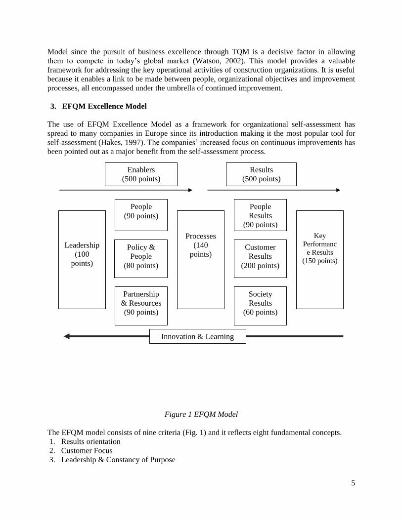
5
Model since the pursuit of business excellence through TQM is a decisive factor in allowing
them to compete in today’s global market (Watson, 2002). This model provides a valuable
framework for addressing the key operational activities of construction organizations. It is useful
because it enables a link to be made between people, organizational objectives and improvement
processes, all encompassed under the umbrella of continued improvement.
3. EFQM Excellence Model
The use of EFQM Excellence Model as a framework for organizational self-assessment has
spread to many companies in Europe since its introduction making it the most popular tool for
self-assessment (Hakes, 1997). The companies’ increased focus on continuous improvements has
been pointed out as a major benefit from the self-assessment process.
Figure 1 EFQM Model
The EFQM model consists of nine criteria (Fig. 1) and it reflects eight fundamental concepts.
1. Results orientation
2. Customer Focus
3. Leadership & Constancy of Purpose
Leadership
(100
points)
People
(90 points)
Policy &
People
(80 points)
Partnership
& Resources
(90 points)
Processes
(140
points)
People
Results
(90 points)
Customer
Results
(200 points)
Society
Results
(60 points)
Key
Performanc
e Results
(150 points)
Innovation & Learning
Enablers
(500 points)
Results
(500 points)

6
4. Management by Processes & Facts
5. Development & Involvement
6. Continuous Learning, Innovation & Improvement
7. Partnership Development
8. Public Responsibility
The left hand side is called as “Enablers” which consists of five criteria. These Enablers are
concerned with how the organization performs various activities. The remaining four criteria
residing on the right side is called as “Results”. Results indicate what the organization is
achieving with respect to different stake holders. The model is a self- assessment tool. The
rationale behind the EFQM Excellence Model is that some causal relationship between eight
fundamental concepts must be reflected in the model as a causal relationship between the
enablers and the result criteria.
The changes in the 2010 version of EFQM model signify an increasing realization of the
importance of society. The weighting of the criterion ‘‘Society’’ increased from 6 per cent to 10
per cent. New fundamental concepts of the EFQM model – viz. ‘‘Leading by vision, inspiration
and integrity’’, ‘‘Achieving balanced results’’, ‘‘Building partnerships’’, and ‘‘Taking
responsibility for a sustainable future’’ – have an increasing sustainability focus. In addition, the
focus of sub-criteria is more explicitly towards human values such as practicing ethics and
transparency in the Leadership criterion, and sustainability in the Strategy criterion, etc. Thus,
new dimensions of excellence towards the sustainability focus are clearly emerging, and their
impact on business will be visible in coming times. The recent changes in the EFQM model
indicate a step forwards in enhancing the weighting of goodwill criteria.
The EFQM excellence award is announced to recognize Europe’s best performing organization
whether it is private, public or non-profit. Only EFQM member can apply for this award. It is
supported by one of the most rigorous assessment processes. To identify the finalists, a team of 4
–8 international experienced managers spend one week on site, or an average of 500 hours per
applicant; reviewing documents, interviewing and analyzing the organization against the EFQM
Excellence Model.
The through assessment and feedback from a team of 100 assessors, jury selected thirteen
nominees for present year. Each nominee presented to an independent jury that decides the level
of recognition for each Finalist. To win the EFQM Excellence Award, an applicant must be able
to demonstrate that their performance not only exceeds that of their peers, but also that they will
maintain this advantage into the future (EFQM Excellence Award, 2012). Out of the 13
nominees, the jury identified one EFQM Award Winner, an organization showing excellent
approaches and results across the entire organization. The Jury decided to name the Robert
Bosch Bamberg Plant, the EFQM Excellence Award Winner 2012. Moreover, another 6
organizations got an EFQM Prize in different categories. The organization which demonstrates
role model behavior in one of the following eight criteria’s is announced to be prize winner for
the EFQM Excellence Award:
1. Leading with Vision, Inspiration & Integrity
2. Managing Processes

7
3. Succeeding through People
4. Adding Value for Customers
5. Nurturing Creativity and Innovation
6. Building Partnerships
7. Taking Responsibility for a Sustainable Future
From the self-assessment process, companies experienced the increased focus on continuous
improvements. The continuous improvement must be linked to an increased focus on employee
involvement and employee satisfaction, as they are the most important drivers for that. Involved
and satisfied employees are a primary concern for companies striving for excellence. The
productivity can be improved by raising the number of suggestions for improvement per
employee per year, and thus involving the employees in the companies search for continuous
improvement.
It is therefore vital for any company to identify the drivers of loyalty and employee satisfaction.
If an organization wishes to improve the loyalty and satisfaction of working employees, it can
concentrate the improvement effort within the relevant enabler criteria from the EFQM
Excellence Model and expect a positive impact on loyalty and employee satisfaction. When
trying to determine the drivers of the criterion “Customer Results” it is advantageous to turn to
another customer satisfaction model-the European Customer Satisfaction Index (ECSI) model as
shown in figure 2 (Kristensen, Martensen, & Gronholdt, 1999).
Figure 2. The ECSI Model
This model is validated in many empirical settings and stipulates that loyalty and customer
satisfaction is generated by four variables: expectations, image, perceived quality of human ware
and perceived quality of hard ware. The impact of image in both customer satisfaction models
indicates that “Society Results” must have an impact on “Customer Results” since sub criterion
under “Society Results” deals with “Society’s perception of the organization”.
Image
Expectations
Perceived
quality of
“hard ware”
Perceived
Value
Customer
Satisfaction
Customer
Loyalty

8
Excellence Model frameworks have different shapes. Most Excellence Models start with the
criterion ‘‘Leadership’’ and end with ‘‘Results’’. Ancient wisdom emphasizes that the ultimate
goal of business is the wellbeing of society. Although the criteria of Excellence Models are
similar, the criterion weighting changes due to external environment and cultural factors. The
study is made with nine criteria to integrate the common learning/contradictions of twenty
Excellence Models and provide the clues to achieve sustainability (Talwar, 2011).
4. The Implementation of Overall Excellence Model within the Manufacturing Company
A sample of ten companies was asked to identify any problems related to the application of the
Overall Excellence model. Information was gathered from five structured interviews and a case
study carried out. The results of this consultation process have been utilized in the production of
a generic model designed to assist manufacturing related organizations in their implementation
of the Overall Excellence Model. The success of business organizations, long-lasting and
sustainable need to be explored empirically.
The Model is designed to be flexible, holistic, dynamic, simple and innovative. The fundamental
advantages of Overall Excellence Model include knowledge management, performance,
learning, partnership, customer focus, results orientation and increased cost effectiveness.
Figure 3: Theoretical Overall Excellence Model
4.1 Customer Satisfaction
In customer satisfaction research, analytic methods are needed to capture the complex
relationship between overall satisfaction with a product or service and the underlying
performance on the product’s or service’s attributes. Eventually, the method should allow
identifying the attributes that need improvement and that most significantly enhance the business
relationship with the customer (Vanhoof, Pauwels, Dombi, Brijs, & Wets, 2005).
Business
Performance
Employee
Satisfaction
Product
Quality
Customer
Satisfaction
Overall Excellence Model
Implementation

9
In prevailing cut throat competition, it is very clear that a company survival depends on its
ability to satisfy customer’s expectations and needs. Quick response to customer complaints on a
product is essential to minimize customer dissatisfaction. The information must be gathered from
surveys regarding competency of product in global market. Intensive examination of finished
products from the customer view point can be useful predictor of customer satisfaction. It may
very well predict the future success or failure of a firm. Thus it is very important to find
customer satisfaction and perception of quality. The maintenance and attainment of satisfactory
levels is today fundamental determination for business growth, economic viability and health.
It can be measured by comparing product quality and service quality with those in other firms in
the same industrial sector. Use of customer satisfaction information can provide a focus and
direction for continuous improvement throughout the entire firm. By delighting the customer you
can turn satisfied customers into loyal customers. Loyalty generates repeated purchases and
increased revenues, thus leading to organizational excellence.
4.2 Employee Satisfaction
One of the key performance measures of a firm is Employee Satisfaction. It is a topic of interest
to both researchers who study it and practitioners who work in firms. It is the extent to which
employees like or dislike their jobs. It is an attitudinal variable and can be considered as a global
feeling about the job. Employee satisfaction is needed to support continuous improvement and
external customer satisfaction. Delighted employees who feel proud of their work have an
outstanding performance, thus having a positive impact on business excellence.
The employee involvement and satisfaction has a positive effect on the organization’s ability to
continuously improve in the competitive market. The productivity can be improved by raising
the number of suggestions for improvement per employee per year, and thus involving the
employees in the companies search for continuous improvement.
4.3 Product Quality
A narrow definition of product is that they are tangible and physical. This is in contrast to
service, which is intangible. In manufacturing processes, conformance to standards is a very
critical aspect. It relates to how closely the final product matches its design specification. The
quality of the final product should not merely rely on the general inspections due to the
complexity of unstable factors in manufacturing process. The errors or variation caused by those
factors could be accumulated gradually in the process and thus avoid serious troubles in the
subsequent stages (Sonigra & Qureshi, 2012). The process performance is estimated by the
quality characteristics of items produced from a process. A process capability index is used as
one of the evaluation measures for process performance.
The quality of process output can be measured in various ways. The percentage of the fraction of
items that does not confirm to specifications is used. In many practical situations it is convenient
to measure the quality of the product or the service by the number of nonconformities per ‘unit
area of opportunity’. Some times the quality of sample of items is measured by the mean of the
measurements or by some other measure of central tendency such as a percentile.

10
Many studies have been conducted to estimate the importance of quality. Some studies have tried
to find a linkage between high products qualities and companies’ financial performances. It
demonstrate that companies that win quality awards outperform other firms on operating income
measures as well as stock performance (Hendricks & Singhal, 2001).
“Total quality control", also called total quality management, is an approach that extends beyond
ordinary statistical quality control techniques and quality improvement methods. It implies a
complete overview and re-evaluation of the specification of a product, rather than just
considering a more limited set of changeable features within an existing product. If the original
specification does not reflect the correct quality requirements, quality cannot be inspected or
manufactured into the product. For instance, the design of a pressure vessel should include not
only the material and dimensions, but also operating, environmental, safety, reliability and
maintainability requirements, and documentation of findings about these requirements.
4.4 Business Performance
The six sigma process is an excellent fit for the fabrication and machining industries. Any
company that needs solutions for quality related problems should benefit from this process.
Companies will be most likely to succeed if their top-level management is supportive of a
continuous improvement culture. Organizations need a framework that is comprehensive,
flexible and easy to adopt. Since success clearly depends on a combination of factors that are
interrelated, the approach must be highlighting and holistic. Any change in one of the
components will have impact on the overall system.
Several studies point out that a focus on customers, employees and business results is a must for
survival in the current economic environment. Increasing globalization, rapid transportation, the
information technology boom and improved communications have enhanced competitiveness
and have further reduced the gap between developed and developing economies. The key
concern of organizations is not just customer satisfaction, but customer retention. Though most
corporate entities make profits, they are not able to retain even half of their customers.
5. Conclusion
The proposed Overall Excellence model offer companies the capability to develop and
implement an effective and dynamic quality system, with a focus on continuous improvement
and adaptation. The real benefits can be realized only when the companies that apply them truly
understand both their capabilities and their limits. The Overall Excellence model is expected to
provide a direction to obtain sustainable profits, people and planet development. It brings
business organizations closer to their truly final objective of long-run satisfaction of the needs
and desires of all stakeholders and the global community.
There are other issues concerning the model, after establishing the causality in the Overall
Excellence model. These issues provides platform for future research. More research is possible
on the simplification this model. It is not possible for any company to get excellence but the
company can strive to attain the excellence. An emerging focus on environmental concerns,

11
inclusive growth, corporate governance and ethical practices, etc., in recent times is an indication
of a paradigm shift towards the growing importance of goodwill criteria (Talwar, 2008).
The structure of learning organization is built on strong foundations of management culture that
implements the right management systems to establish deep knowledge through leadership and
employee professional development, which ensure business survival and growth through quality
focus and excellence. This should be harmonized with society benefit, embracing also
environmental protection and resources management toward sustainable development
(Pantazopoulos, 2012).
At present, manufacturers are facing an increasingly uncertain external environment with a
cumulative effect of changes in customer requirements, global competition, and technological
advancement. Manufacturers face the challenge of improving efficiency and lowering costs. QC
techniques would be continuously exploited to help organizations to improve their products and
process in order to be accepted by customers.
The long term effectiveness and real value of the quality assurance standards are not based on
their content and requirements, but on the way that these are adopted and implemented by the
companies. The key for their success lies in the companies’ real commitment to quality
improvement and their true motives for certification, which finally dictate the way and depth to
which the standards are implemented. The firm may develop its own specific measurement
system that can better measure employee satisfaction, product quality, customer satisfaction, and
strategic business performance. Though several initiatives have taken place in past four decades
to attain excellence, some of the software criteria have still not yet gained adequate focus. A lack
of focus on human values gives rise to the risk of the use of unethical practices to maximize
short-term gains. Financial scandals at large multinational corporations such as Enron and
WorldCom have brought the need for ‘‘ethical’’ management into focus. Vedic philosophy and
other religious texts emphasizes that one should work not for own self only, but for universal
wellbeing, also.
6. References
The Deming Prize. (2010). Retrieved from www.juse.or.jp: www.juse.or.jp/deming/index.html
EFQM Excellence Award. (2012, September 26). Retrieved Oct 1, 2012, from www.efqm.org:
http://www.efqm.org/en/Home/tabid/36/Default.aspx
Abbasi, B., Taghi, S., & Niaki, A. (2010). Estimating process capability indices of multivariate
nonnormal processes. International Journal of Manufacturing Technology, 823-830.
Gouda, S. A., Zhang, W., & Haridy, S. (2011). An integrated framework of Statistical Process
Control and design of experiments for optimizing wire electrochemical turning process.
International Journal of Advanced Manufacturing Technology 53, 191-207.
Hairulliza, M. J., Ruzzakiah, J., & Genasan, D. (2011). Motivating Factors and Challanges,
Applications and Experiences of Quality Control. Quality Control Implementation in
Manufacturing Companies, 495-508.
Hakes, C. (1997). The Corporate Self Assessment Handbook. London: Chapman Hall.
Hendricks, K. B., & Singhal, V. R. (2001). The long-run stock price performance of firms with
effective TQM programs. Management Science, Vol.47, No.3, 359-368.

12
Institute, N. Q. (2007). Canada Awards for Excellence. www.nqi.ca/caeawards: Natio.
Kanter, R. M., & Page, G. R. (2011). Baldridge 2020 : An Executive's Guide to the Criterial for
Performance Excellence. Geithersburg, USA: NIST.
Katerina, G. D., & George, T. D. (2001). An empirical study of the ISO 9000 standards'
contribution towards total quality management. International Journal of Operations &
Production Management, Vol.21, No.10, 1326-1342.
Kristensen, K., Martensen, A., & Gronholdt, L. (1999). Measuring the impact of buying
behaviour on customer satisfaction. Total Quality Management Vol. 10, 4-5.
Pantazopoulos, G. A. (2012). Failure Analysis, Quality Assurance, and Business Excellence.
Journal of Failure Analysis and Prevention, 50-63.
Qureshi, M. N., & Sonigra, S. S. (2010). Application of SPC Tools in Maintenance Management.
4th International Conference on Advances in Mechanical Engineering (pp. 518-523).
Surat: SVNIT.
Reichheld, F. F. (1990). Zero defections: quality comes in service. Harvard Business Review.
Sonigra, S. S., & Patel, K. S. (2009). Statistical Process Control Analysis of critical parameters
of connecting rod of I. C. Engine. Emerging Trends in Mechanical Engineering (pp. 50-
55). Vallabh Vidyanagar: ETME2009.
Sonigra, S. S., & Qureshi, M. N. (2010). Examining the influence of temperature variation on
dimensional variability of connecting rod. 2nd International Conference on Production
and Industrial Engineering (pp. 1435-1442). Jalandhar: NIT.
Sonigra, S. S., & Qureshi, M. N. (2012). Solving the Problem of End Float with the Application
of Six Sigma Tools: A Case Study. The IUP Journal of Mechanical Engineering, Vol. V,
No.2, 7-20.
Talwar, B. (2008, April). Evolultion of 'Universal Business Excellence Model' incorporating
Vedic philosophy. Ph. D. Thesis. Roorkee: Indian Institute of Technology.
Talwar, B. (2011). Comparative study of framework, criteria and criterion weighting of
excellence models. Measuring Business Excellence, Vol. 15, 49-65.
Technology, N. I. (2009). 2009-2010 criteria for performance excellence .
http://baldrige.nist.gov: Baldrige National Quality Program.
Vanhoof, K., Pauwels, P., Dombi, J., Brijs, T., & Wets, G. (2005). Penalty-Reward Analysis
with Uninorms: A Study of Customer (Dis)Satisfaction. Intellegent Data Mining Studies
in Computational Intellegence, 237-252.
Watson, P. (2002). Implementing the European Foundation for Quality Management Excellence
Model. TS1.1 Business Practices (pp. 1-18). Washington, D.C. USA: FIG XXII
International Congress.
Westerveld, E. (2003). The Project Excellence Model : linking success criteria and critical
success factors. International Journal of Project Management, 411-418.