JournalofGeophysicalResearch: SolidEarth

RESEARCHARTICLE10.1002/2013JB010282

Key Points:• Elastic heterogeneity causes strongCoulomb stress fluctuation of powerlaw type

• Gutenberg-Richter relation resultsfrom power law fluctuations ofCoulomb stress

• Universal fractal nature of elasticheterogeneity suggests a universalb value

Correspondence to:C. Langenbruch,Cornelius@geophysik.fu-berlin.de

Citation:Langenbruch, C. and S. A. Shapiro(2014), Gutenberg-Richter relation orig-inates from Coulomb stress fluctuationscaused by elastic rock heterogene-ity, J. Geophys. Res. Solid Earth, 119,doi:10.1002/2013JB010282.

Received 12 APR 2013

Accepted 19 JAN 2014

Accepted article online 28 JAN 2014

Gutenberg-Richter relation originates from Coulomb stressfluctuations caused by elastic rock heterogeneityC. Langenbruch1 and S. A. Shapiro1

1Fachrichtung Geophysik, Freie Universität Berlin, Berlin, Germany

Abstract Based on measurements along boreholes, a characterization of the Earth’s crust elasticheterogeneity is presented. We investigate its impact on Coulomb stress distribution and earthquakemagnitude scaling. The analysis of elastic modulus distribution at various borehole locations in differentregions reveals universal fractal nature of elastic heterogeneity. By applying a homogeneous far-field stressto a representativemodel of elastic rock heterogeneity, we show that it causes strong Coulomb stressfluctuations. In situ fluctuations of Coulomb stress are mainly controlled by in situ elastic moduli.Fluctuations caused by surrounding heterogeneities are only of minor importance. Hence, the fractalnature of elastic heterogeneity results in Coulomb stress fluctuations with power law size distribution. As aconsequence, fault sizes and magnitudes of earthquakes scale according to the Gutenberg-Richterrelation. Due to the universal fractal nature of elastic heterogeneity, the b value should be universal.Deviation from its universal value of b ≈1 occurs due to characteristic scales of seismogenic processes,which cause limitations or changes of fractal scaling. Scale limitations are also the reason for observedstress dependency of the b value. Our analysis suggests that the Gutenberg-Richter relation originates fromCoulomb stress fluctuations caused by elastic rock heterogeneity.

1. Introduction

Sonic well logs provide in situ measurements of physical properties and their fluctuations in the Earth’s crust.The analysis of collected log data has contributed to the characterization of elastic rock heterogeneity, sinceit proved its fractal nature [see, e.g., Leary, 1997; Dolan et al., 1998; Goff and Holliger, 1999]. Stress measure-ments along boreholes show that stress in the Earth’s crust shows significant spatial heterogeneity [see, e.g.,Brudy et al., 1997; Hickman and Zoback, 2004; Day-Lewis et al., 2010]. Consistently, a stress inversion studyusing earthquake mechanisms by Rivera and Kanamori [2002] suggests that stress unlikely is uniform in ori-entation or magnitude. Moreover, results of stress orientation analysis from borehole breakouts argue for afractal nature of existing stress fluctuations [Day-Lewis et al., 2010]. Even though it is evident that elastic het-erogeneity of rocks naturally results in a fluctuating stress field, its impact on stress in rocks has not yet beencharacterized. Does elastic heterogeneity have a significant influence on stress at all? If so, does the frac-tal distribution of elastic moduli cause stress variations with power law size distribution? This would be ofgreat importance, since it has been shown that fractal fluctuations result in power law scaling of earthquakemagnitudes, expressed by the Gutenberg-Richter relation [Gutenberg and Richter, 1954; Huang and Turcotte,1988]. In this paper, we analyze relations between elastic rock heterogeneity, stress fluctuations, and theGutenberg-Richter b value of earthquakes. We start with a characterization of the Earth’s crust elastic het-erogeneity by analyzing sonic logs along the Continental Deep Drilling Site (KTB) main hole. Using derivedparameters of elastic modulus distribution, we simulate an elastically heterogeneous 3-D randommediumcharacterized by a power spectrum of fluctuations of power law type. The simulatedmedium is statisticallyequivalent to the log data and represents the rock surrounding the borehole.

We apply an externally homogeneous far-field stress and compute stress fluctuations inside the model. Theexternally applied stress field is determined from smoothed stress profiles along the KTB main hole [seeIto and Zoback, 2000]. In the next section, we interpret the occurring stress fluctuations in terms of fracturestrength variations by determining the distribution of Coulomb failure stress (CFS) as a measure of fracturestrength in rocks. In the final part, we analyze the scaling behavior of fracture strength distribution rep-resented by the CFS. Aki [1981] describes the assemblage of faults by the concept of fractals and showsthat the Gutenberg-Richter relation is equivalent to a fractal distribution of fracture sizes. The power lawexponent of fault size distribution is equivalent to the b value of earthquakes, describing the ratio between

LANGENBRUCH AND SHAPIRO ©2014. American Geophysical Union. All Rights Reserved. 1

Journal of Geophysical Research: Solid Earth 10.1002/2013JB010282

small- and large-magnitude earthquakes. Assuming that rupturing, once it is initiated (e.g., by an increase instress or pore pressure), takes place inside isosets of Coulomb failure stress (CFS≤ constant), we determinethe scaling exponent of resulting fracture sizes and compare it to the b value. To characterize solely the influ-ence of measurement-based elastic rock heterogeneity, we restrict the analysis to a static view and excludeassumptions about dynamic interaction of fractures; that is, we neglect stress fluctuations caused by possi-ble seismic events on corresponding critically stressed isosets. Our modeling of the stress distribution in 3-Dheterogeneous elastic structures is a minimum-assumption first-principle approach. It takes into accountany type of interaction (i.e., multiple scattering) between elastic heterogeneities.

Laboratory studies [Mogi, 1962; Scholz, 1968; Amitrano, 2003], observations [Schorlemmer et al., 2005], andmodeling [Huang and Turcotte, 1988] suggest that the b value is not universal. Generally, a positive rela-tion to the degree of rock heterogeneity complexity and an inverse relation to the level of differentialstress is observed. The fractal dimension of elastic modulus distribution can be related to the degree ofmaterial heterogeneity complexity, because it describes the relation between large- and small-scale corre-lated structures. Therefore, we investigate if the range of theoretically possible fractal dimensions of elasticheterogeneity can explain observed b value variations.

Day-Lewis et al. [2010] find that the scaling behavior of physical property heterogeneity derived from welllogs is universal. We investigate the scaling behavior of elastic heterogeneity at different drilling sites toanalyze if the scaling of elastic rock heterogeneity and resulting CFS fluctuations in our model can be con-sidered as universally valid. Thereafter, we discuss the importance of the finding that the fractal dimensionof elastic heterogeneitymeasured from well logs at various drilling sites seems to be universal. Finally, weanalyze relations between stress level and b value resulting from our model and argue that deviation of theb value from its universal value of b ≈ 1 results from characteristic scales of seismogenic processes, whichcause limitations or changes of fractal scaling.

The analysis presented in this paper will lead to the following main findings: Elastic rock heterogeneityis of fractal nature and causes strong Coulomb failure stress fluctuations with power law size distribu-tion. The fractal scaling of the Coulomb stress fluctuations, in turn, explains the emergence of earthquakemagnitude scaling according to the Gutenberg-Richter relation. Because the fractal dimension of elasticheterogeneity, determined from log data at various drilling sites in different regions, is more or less uni-versal, the b value should be universal. Deviations of the b value from its universal value of b ≈ 1 resultonly from characteristic scales of seismogenic processes, which cause limitations or changes of fractal scal-ing. Scale limitations are also the reason for observed stress dependency of the b value. These findings areunaffected by instrumental and measurement effects on the fractal dimension, because we can expect astatistically similar impact at different analyzed locations. Hence, the universality issue should remainmainly untouched.

We start the analysis by characterizing elastic rock heterogeneity of the Earth’s crust based on soniclog measurements.

2. Characterization of Elastic Heterogeneity in the Earth’s Crust

In this section, we characterize elastic heterogeneityof the Earth’s crust by analyzing sonic log data collectedalong the Continental Deep Drilling site KTB-1 main hole located in southeastern Germany [see, e.g., Pechniget al., 1997]. We evaluate the depth section between 4450m and 6017m in the crystalline basement. Thissection is selected for the analysis, because fluid injected during an injection operation in the year 2000stimulated the rock formation at this depth and induced numerous seismic events [see Baisch et al., 2002].The occurrence of seismic events indicates that the state of stress in this depth section is close to a criticalone causing brittle failure of rocks.

Figures 1a and 1b show shear (𝜇) and bulk (K) moduli computed from 4m averaged P and Swave travel timeand density logs along the KTB-1 main hole. We averaged the raw data (sampled at 0.152m) in 4m inter-vals to eliminate inherent averaging of the logging process over the active length of the tool (≈ 1m) and toreduce high-frequency noise. The distributions of 𝜇 and K with depth are highly heterogeneous. Two nar-row layers of paragneisses cut the metabasitic basement in depth sections 5210–5310 m and 5540–5640 m[Pechnig et al., 1997]. The moduli in these depth sections are characterized by lower mean values, resulting

LANGENBRUCH AND SHAPIRO ©2014. American Geophysical Union. All Rights Reserved. 2

Journal of Geophysical Research: Solid Earth 10.1002/2013JB010282

Figure 1. Characterization of elastic heterogeneity along the KTB main hole. (a, b) Shear and bulk moduli computed from 4m averaged P and S wave travel time and density logsalong the KTB-1 main hole. Grey shaded areas indicate gneiss layers [see Pechnig et al., 1997], which we exclude from the analysis. (c, d) Probability density function (PDF) of 𝜇 and Kobtained from Figures 1a and 1b. (e) Cross plot of 𝜇 and K values. (f ) Cross plot of simulated random number pairs representing shear and bulk moduli. (g, h) Power spectral densityfunction (PSDF) of 𝜇 and K log data.

in nonstationary statistics of the distribution. We exclude these layers from our analysis to ensure statisticalstationarity of elastic parameter distribution.

We now determine the statistical parameters describing the distribution of shear and bulk moduli and cre-ate a randommedium, which is statistically equivalent to the log data. This medium will represent the rocksurrounding the borehole. Since we exclude the paragneiss layers from our analysis, the model will rep-resent elastic heterogeneity occurring in one single type of rock. Figures 1c and 1d show the probabilitydensity functions (PDF) of shear and bulk moduli. We determine best fitting Gaussian distributions to obtainmean values (< 𝜇 >= 35.0 GPa, < K >= 70.7GPa) and standard deviations (𝜎

𝜇= 3.4GPa, 𝜎K = 7.1GPa).

Similarities between the distributions of 𝜇 and K with depth are visible in the logging data (see Figures 1aand 1b). This indicates a positive relation between both moduli. To analyze this relation in more detail, wepresent a cross plot of 𝜇 and K in Figure 1e. The moduli indeed show a positive relation, which we quantifyby calculating Pearson’s correlation coefficient Pc given by the covariance of 𝜇 and K divided by the prod-uct of their standard deviations. The moduli show a strong positive correlation quantified by Pc

𝜇,K = 0.64.We then apply the obtained mean values, standard deviations, and the correlation coefficient to simulatecorrelated random number pairs representing bulk and shear moduli. A cross plot of simulatedmoduli ispresented in Figure 1f. Random assignment to a 3-D medium consisting of 100×100×100 equally sized cellsresults in two related spatially uncorrelatedmedia (see Figure 2a). These media represent the distribution ofelastic moduli in space.

However, real rocks show spatial correlations of elastic properties. Data analysis from various drilling sitessuggests unbounded fractal scaling of the Earth’s crust heterogeneity. This is expressed in power law (k−𝛽 )dependence of the log data’s power spectra on the wave number k [Leary, 1997]. The scaling exponent 𝛽 isgiven by

𝛽 = 2H + E, (1)

where E is the Euclidean dimension and H is the Hurst exponent, which can be related to the fractaldimensionD of the log data by [see, e.g., Dolan et al., 1998]

D = (E + 1) − H. (2)

LANGENBRUCH AND SHAPIRO ©2014. American Geophysical Union. All Rights Reserved. 3

Journal of Geophysical Research: Solid Earth 10.1002/2013JB010282

Figure 2. Random medium realizations. (a) Related spatially uncorrelated media representing shear (top) and bulk (bottom)moduli. The media result from a random assignment of simulated shear and bulk modulus pairs shown in Figure 1f. The spa-tial correlation according to a PSDF of power law type results in media with fractal dimension of (b) D𝜇,K = 3.1, (c)D𝜇,K = 3.5, and (d) D𝜇,K = 3.87. The media shown in Figure 2d represent the rock surrounding the KTB-1 bore-hole and are used for further modeling. The figure shows that the fractal dimension D is a measure for the degree of rockheterogeneity complexity.

In general, H can show values in the range 0 ≤ H ≤ 1. Roughness of a fractal distribution is related to H,where higher values of H correspond to smoother distributions.

The power spectral densities of shear and bulk modulus logs at the KTB (see Figures 1g and 1h) possesspower law dependence on the wave number in the complete range. Power law exponents 𝛽 , which aredetermined by the slope of the power spectral density in the double logarithmic representation (Figures 1gand 1h), are given by 𝛽

𝜇= 1.29 (H

𝜇= 0.145) for shear modulus and 𝛽K = 1.24 (HK = 0.12) for bulk modulus.

Because these values are obtained from 1-D sonic logs, the Euclidean dimension of a line (E = 1) is used forcomputation of the Hurst exponents according to equation (1). The low values of H are in agreement withobservations of Day-Lewis et al. [2010]. They observe that a power law exponent of 𝛽 ≈ 1 is typical for phys-ical property scaling derived from sonic well logs at various sites. The observed low values of H stand for ahigh degree of heterogeneity complexity of elastic properties.

We now use the determined Hurst exponents to spatially correlate the simulated distributions of 𝜇 andK shown in Figure 2a. Because the power law exponents of K and 𝜇 can be considered as equivalent, weapply fractal scaling according to a Hurst exponent H = 0.13 to both media. The value of H = 0.13 cor-responds to the mean value of H𝜇 and HK . Since we do not have any information about elastic propertyscaling in horizontal direction, we assume that Hurst exponents in vertical and horizontal direction are thesame. Even though the Hurst exponent in sedimentary rocks may vary from vertical to horizontal direction,it should be approximately equal in the granite basement. Spatial correlation is obtained by filtering themedia in the wave number domain. More precisely, the Fourier transforms of spatially uncorrelated shearand bulk modulus distributions are multiplied by the square root of the fractal power spectral density func-tion PSDF(k) = k−𝛽 , in the wave number domain, where k =

√k2x+ k2

y+ k2

zis the wave number. Since we

assign a distribution to a 3-D medium, the Euclidean dimension is given by E = 3. Considering the relationof 𝛽 = 2H + E and the computed Hurst exponent of H = 0.13, we apply a power law exponent of 𝛽 = 3.26to spatially correlate the media. By taking the inverse Fourier transform, we obtain the fractal randommediain the spatial domain. Considering the relation D = (E + 1) − H, the resulting distributions of 𝜇 and K (seeFigure 2d) are characterized by a fractal dimension of D

𝜇,K = 3.87.

The simulated media (see Figure 2d) are representing the distribution of 𝜇 and K around the borehole,because they are statistically equivalent to the log data; that is, they show the same mean values, standard

LANGENBRUCH AND SHAPIRO ©2014. American Geophysical Union. All Rights Reserved. 4

Journal of Geophysical Research: Solid Earth 10.1002/2013JB010282

−200

0

200

−200

0

200−200

0

200

z[m]x[m]

y[m

]

155

160

165

170

175

180

185

190

195

200

205

MPa

yy

−200

0

200

−200

0

200−200

0

200

z[m]x[m]

y[m

]

80

85

90

95

100

MPa

zz

−200

0

200

−200

0

200−200

0

200

z[m]x[m]

y[m

]

38

40

42

44

46

48

50

52

54

MPa

xx

Figure 3. Stress modeling results: Normal stress component in y(𝜎1e), z(𝜎2e), and x(𝜎3e) directions. The color bars are scaled to ±20% ofthe externally applied stresses. The directions of externally applied principal stresses are shown at the top of the figures. Due to elasticheterogeneity, stress strongly fluctuates inside the medium.

deviations, and correlation coefficient between K and 𝜇. Moreover, the values along any 1-D profile in thesimulatedmedia possess a fractal dimension of 1.87 (H = 0.13), which is equivalent to the fractal dimensionof the log data. In general, the fractal dimension of a distribution applied to a 3-D medium (E = 3) is in therange of 3 ≤ D ≤ 4. This becomes clearer by considering that the fractal dimensions of a distribution appliedto a line (E = 1), for instance, well log data, can possess fractal dimensions of 1 ≤ D ≤ 2.

Again, we note that fields of elastic properties are heterogeneously distributed in the real three-dimensionalspace (E = 3) by their power spectra (i.e., their spatial correlation functions). These fields represent frac-tals in a space of the embedding dimension 4. The fourth dimension is given by the color in our figures.Corresponding fractals have fractal dimension between 3 and 4. The fractal dimension of the media sim-ulated according to the well log data along the KTB main hole are characterized by a fractal dimension ofD𝜇,K = 3.87. Figures 2b and 2c show fractal media characterized by lower fractal dimensions of D𝜇,K = 3.1and D𝜇,K = 3.5, respectively. The figure illustrates that the fractal dimension describes the relation of small-to large-scale structures and can be related to the degree of rock heterogeneity complexity.

3. Stress Fluctuations in Elastically Heterogeneous Rocks

In this section, we analyze stress fluctuations resulting from elastic rock heterogeneity and establish rela-tions between stress fluctuations and elastic properties. Therefore, the medium realization of elastic moduli(Figure 2d) is used as input to a finite element stress analysis model. We use the commercial software pack-age ABAQUS. An externally homogeneous far-field stress is applied to determine the distribution of stressinside the elastically heterogeneous rock model. Compressive stresses are always defined positive in thefollowing. We consider smoothed stress profiles reported by Ito and Zoback [2000]: SH = 0.045MPa/m,SV = 0.028MPa/m, and Sh = 0.02MPa/m. The stress profiles are derived from hydraulic fracturing tests,breakouts, and drilling-induced fractures along the KTB main hole. A strike-slip stress regime is prevail-ing, and the differential stress is increasing with depth [Brudy et al., 1997]. We calculate effective principalstresses, considering a hydrostatic pore pressure gradient of 0.0115MPa/m, reported by Huenges et al.[1997] along the KTB main hole up to a depth of 9.1 km. The principal stress components of the externallyapplied stress field are defined at the corresponding boundary surfaces of the model medium as follows:𝜎1e = 180.9 MPa = 𝜎yy , 𝜎2e = 89.1 MPa = 𝜎zz , and 𝜎3e = 45.9 MPa = 𝜎xx . These values correspondto maximum horizontal, vertical, and minimum horizontal effective principal stresses at a depth of 5.4 km.Again, we note that we consider this depth since a fluid injection in the year 2000 induced seismic eventsin this depth range. By evaluation of the ABAQUSmodel, we obtain the full stress tensor in each model cell.Figure 3 shows the resulting normal stress components in y(𝜎1e), z(𝜎2e), and x(𝜎3e) directions. In the case ofan elastically homogeneous medium the stress components would coincide with the externally appliedstresses 𝜎1e , 𝜎2e , and 𝜎3e in all cells of the model. It means that the stress inside a homogeneous mediumis independent of the elastic properties of the medium. However, as soon as the medium becomes elasti-cally heterogeneous, stress fluctuations occur, which are controlled by the deviations of elastic propertiesfrom their mean values. We find that elastic heterogeneity has a significant influence on stress magnitudes,which vary by up to more than ±20% of the externally applied stresses. We note that the directions of

LANGENBRUCH AND SHAPIRO ©2014. American Geophysical Union. All Rights Reserved. 5

Journal of Geophysical Research: Solid Earth 10.1002/2013JB010282

−200

0

−200

0

200−200

200

z[m]

5

10

15

20

0 5 10 15 20 250

1

2

3

4

5

6x 10

4

CFS [MPa]

num

ber

of c

ellsCFS

a)

y[m]

x[m] MPa

b)

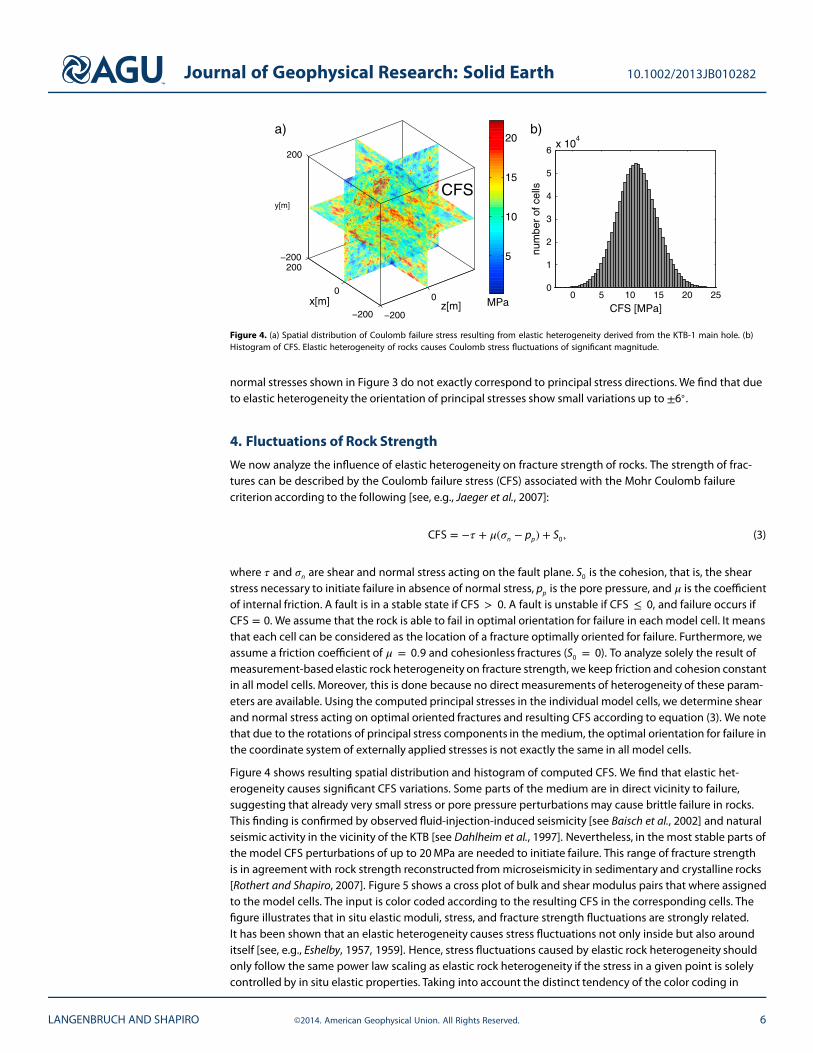
Figure 4. (a) Spatial distribution of Coulomb failure stress resulting from elastic heterogeneity derived from the KTB-1 main hole. (b)Histogram of CFS. Elastic heterogeneity of rocks causes Coulomb stress fluctuations of significant magnitude.

normal stresses shown in Figure 3 do not exactly correspond to principal stress directions. We find that dueto elastic heterogeneity the orientation of principal stresses show small variations up to ±6◦ .

4. Fluctuations of Rock Strength

We now analyze the influence of elastic heterogeneity on fracture strength of rocks. The strength of frac-tures can be described by the Coulomb failure stress (CFS) associated with the Mohr Coulomb failurecriterion according to the following [see, e.g., Jaeger et al., 2007]:

CFS = −𝜏 + 𝜇(𝜎n − pp) + S0, (3)

where 𝜏 and 𝜎n are shear and normal stress acting on the fault plane. S0 is the cohesion, that is, the shearstress necessary to initiate failure in absence of normal stress, pp is the pore pressure, and 𝜇 is the coefficientof internal friction. A fault is in a stable state if CFS > 0. A fault is unstable if CFS ≤ 0, and failure occurs ifCFS = 0. We assume that the rock is able to fail in optimal orientation for failure in each model cell. It meansthat each cell can be considered as the location of a fracture optimally oriented for failure. Furthermore, weassume a friction coefficient of 𝜇 = 0.9 and cohesionless fractures (S0 = 0). To analyze solely the result ofmeasurement-basedelastic rock heterogeneity on fracture strength, we keep friction and cohesion constantin all model cells. Moreover, this is done because no direct measurements of heterogeneity of these param-eters are available. Using the computed principal stresses in the individual model cells, we determine shearand normal stress acting on optimal oriented fractures and resulting CFS according to equation (3). We notethat due to the rotations of principal stress components in the medium, the optimal orientation for failure inthe coordinate system of externally applied stresses is not exactly the same in all model cells.

Figure 4 shows resulting spatial distribution and histogram of computed CFS. We find that elastic het-erogeneity causes significant CFS variations. Some parts of the medium are in direct vicinity to failure,suggesting that already very small stress or pore pressure perturbationsmay cause brittle failure in rocks.This finding is confirmed by observed fluid-injection-induced seismicity [see Baisch et al., 2002] and naturalseismic activity in the vicinity of the KTB [see Dahlheim et al., 1997]. Nevertheless, in the most stable parts ofthe model CFS perturbations of up to 20MPa are needed to initiate failure. This range of fracture strengthis in agreementwith rock strength reconstructed frommicroseismicity in sedimentary and crystalline rocks[Rothert and Shapiro, 2007]. Figure 5 shows a cross plot of bulk and shear modulus pairs that where assignedto the model cells. The input is color coded according to the resulting CFS in the corresponding cells. Thefigure illustrates that in situ elastic moduli, stress, and fracture strength fluctuations are strongly related.It has been shown that an elastic heterogeneity causes stress fluctuations not only inside but also arounditself [see, e.g., Eshelby, 1957, 1959]. Hence, stress fluctuations caused by elastic rock heterogeneity shouldonly follow the same power law scaling as elastic rock heterogeneity if the stress in a given point is solelycontrolled by in situ elastic properties. Taking into account the distinct tendency of the color coding in

LANGENBRUCH AND SHAPIRO ©2014. American Geophysical Union. All Rights Reserved. 6

Journal of Geophysical Research: Solid Earth 10.1002/2013JB010282

Figure 5. Cross plot of elastic input moduli of stress modeling. Themarkers are color coded according to the CFS in the corresponding cells.A clear relation between elastic input parameters and the Coulombstress fluctuations is visible by the distinct trend of color coding. Insitu Coulomb stress is mainly controlled by in situ elastic moduli. Stresschanges caused by surrounding heterogeneities are existent and visi-ble by the scatter in the tendency of color coding. However, this effectseems to be only of minor importance.

Figure 5, it becomes clear that in situ stressis mainly controlled by in situ elastic moduli,where the strength of CFS fluctuation is con-trolled by the deviation of elastic propertiesfrom their mean values. Stress changes causedby surrounding heterogeneities are existentand visible by the scatter in the tendency ofcolor coding. However, this effect seems to beonly of minor importance. In general, cells char-acterized by a low bulk modulus and a highshear modulus are in a stress state close to fail-ure. The fracture strength represented by theCFS is systematically increasing with increasingbulk modulus and decreasing shear modulus.Failure will hence most likely occur in partsof a rock characterized by low bulk modulusand high shear modulus, while parts of highbulk modulus and low shear modulus will actas barriers for fracture propagation. The directrelation between in situ elastic properties andCFS suggests that elastic heterogeneity causes

stress fluctuations of power law type. We analyze scaling behavior of CFS and its implications for earthquakemagnitudes scaling in the next section.

5. EarthquakeMagnitude Scaling

Considering the fact that zones of failure in rocks are not continuous planes but exhibit self-similar fragmen-tation at all scales, Aki [1981] describes the assemblage of faults using the concept of fractals. Assuming thatM0 ∝ A

32 and log(M0) ∝

3

2M [see Kanamori and Anderson, 1975], whereM0 is the seismic moment, A is the

fault area andM is the magnitude, the Gutenberg-Richter relation [see Gutenberg and Richter, 1954]

log(NM) = a − bM (4)

can be expressed in the following form [see Aki, 1981]:

log(NM) = a − b log(A). (5)

The constants a and b characterize earthquake productivity and the ratio between small- andlarge-magnitude earthquakes, respectively. The Gutenberg-Richter relation in the form of equation (5) sug-gests that the power law exponent of fault size distribution is equivalent to the b value of earthquakes. Wenow analyze if fracture sizes resulting from our model of elastic heterogeneity possess power law scalingand a scaling exponent similar to the b value of earthquake.

Failure will occur in all critically stressed cells characterized by CFS ≤ 0. Causes of a CFS decrease are, forinstance, tectonic loading and an increase in pore pressure resulting from a fluid injection or ascendingcrustal fluids. In the most simple case of a constant CFS decreaseΔCFS in the completemedium, the isosetCFS(x, y, z) ≤ ΔCFS defines the number size distribution of faults and accordingly magnitude scaling. Toanalyze solely the result of measurement-based elastic rock heterogeneity, we do not introduce assump-tions about dynamic interaction of fractures during the failure process and assume that all faults are formedsimultaneously; that is, we neglect stress fluctuations caused by possible seismic events on correspondingcritically stressed isosets. Our analysis is a minimum-assumption first-principle approach. Each single closedcluster of interconnectedcritically stressed cells represents one fault. In the previous section we have shownthat the CFS is strongly related to the fractal distribution of elastic properties. Therefore, the fluctuations ofCFS should also possess fractal scaling. Consequently, scaling of fault sizes is explicitly defined by the fractaldimensionDi of the isoset: CFS(x, y, z) ≤ ΔCFS. Again, we note that fields of elastic properties, distributedheterogeneously in the real three-dimensional space (E = 3), are embedded in dimension 4. The fourthdimension is given by the color in our figures. Corresponding fractals have fractal dimension between 3

LANGENBRUCH AND SHAPIRO ©2014. American Geophysical Union. All Rights Reserved. 7

Journal of Geophysical Research: Solid Earth 10.1002/2013JB010282

0 1 2 3 40

0.5

1

1.5

2

2.5

3

3.5

4

log10

(number of cells)

log 10

(cum

ulat

ive

num

ber)

modeling results: scaling of fault sizes

scaling of earthquake magnitudes: b=1

Figure 6. Fault size and magnitude scaling: Statistics of critically stressed clusters after a uniform CFS decrease of 5MPa in the complete model medium. (left) Histogram of CFS.(middle) Fracture assemblage resulting from all cells characterized by CFS ≤ 0. (right) Cumulative size distribution of critically stressed clusters. As discussed above the logarithm ofthe number of cells (x axis) represents earthquake magnitudes. Elastic heterogeneity results in magnitudes scaling according to the Gutenberg-Richter relation with b value of b ≈ 1.

and 4. If the distribution of CFS resulting from fields of elastic properties shows fractal scaling, the rangeof possible fractal dimensions of CFS distribution (DCFS) is given by 3 ≤ DCFS ≤ 4. Fractal dimensions ofisosets CFS(x, y, z) ≤ ΔCFS are embedded in the real three-dimensional space. They have fractal dimensionsbetween 2 and 3. This is in agreement with Isishenko and Kalda [1991] who show that an isoset of a frac-tal distribution again is a fractal with fractal dimension of 1 unity less than the fractal distribution itself. Thebasic definition of a fractal distribution is given by

N = crD, (6)

where N is the number of objects with a linear dimension equal to or greater than r, D is the fractal dimen-sion of the distribution, and c is a constant of proportionality [see, e.g., Huang and Turcotte, 1988]. Thus,the number of clusters Nj characterized by a volume equal to or larger than a given volume Vj , that is, thenumber of clusters consisting of j or more interconnectedcritically stressed cells, is given by

Nj = c V−Di3

j

log(Nj) = c −Di

3log(Vj), (7)

whereDi = DCFS−1 is the fractal dimension of the isoset CFS(x, y, z) ≤ ΔCFS, and DCFS is the fractal dimensionof the CFS distribution. The constant c is given by the number of all clusters and is related to the a value ofthe Gutenberg-Richter relation. Since the limits of the fractal dimension of the CFS distribution are given by3 ≤ DCFS ≤ 4, Di is in the range of 2 ≤ Di ≤ 3. If we consider that failure takes place in all cells of a cluster, thefault area is proportional to the number of cells. This assumption presumes very complex fracture surfaces.Correspondingly, magnitudes will be proportional to the logarithm of the number of cells. Comparison ofequations (5) and (7) results in a b value given by

b =Di

3=

DCFS − 1

3. (8)

Accordingly, the b value will be in the range of 2

3≤ b ≤ 1, since the limits of the fractal dimension of CFS

are given by 3 ≤ DCFS ≤ 4. If the CFS distribution is characterized by a fractal dimension equivalent to thefractal dimension of elastic modulus distribution (D

𝜇,K = 3.87), fault sizes should scale with a b value ofb = D𝜇,K−1

3= 0.96.

Figure 6 presents the CFS histogram, fracture assemblage, and cumulative size distribution of criticallystressed clusters resulting from a uniform CFS decrease of |ΔCFS| = 5MPa in the completemodel medium.The size distribution is derived by implementation of a flood fill algorithm. A decrease of 5MPa is appliedto assure a statistically significant number of failing cells. All cells characterized by CFS ≤ 0 contribute tothe fracture assemblage shown in Figure 6 (middle). As discussed above, the logarithm of the number ofcells in the individual clusters of critically stressed cells (x axis of Figure 6, right) represents earthquake mag-nitudes. Resulting fault sizes exhibit power law scaling. Furthermore, the power law exponent of fault sizescaling is remarkably similar to the b value of earthquakes, which is usually given by b≈1. A b value of b≈1

LANGENBRUCH AND SHAPIRO ©2014. American Geophysical Union. All Rights Reserved. 8

Journal of Geophysical Research: Solid Earth 10.1002/2013JB010282

0 1 2 3 40

0.5

1

1.5

2

2.5

3

3.5

4

log 10

(cum

ulat

ive

num

ber)

3.2 3.4 3.6 3.80.4

0.5

0.6

0.7

0.8

0.9

1

log10(number of cells) Dμ,K

b−va

lue

Dμ,K=3.1 Dμ,K

=3.2 Dμ,K=3.3 Dμ,K

=3.4 Dμ,K=3.5 Dμ,K

=3.6 Dμ,K=3.7 Dμ,K

=3.8 Dμ,K=3.9

increasing degree of heterogeneity complexity

b)a)

Figure 7. Influence of the fractal dimension of elastic parameter distribution (D𝜇,K ) on fault size scaling. (a) Cumulative number sizedistributions resulting from stress modeling with input fractal dimension D𝜇,K ranging from 3.1 to 3.9. The figure shows fault sizescomputed for CFS decrease of ΔCFS = 5MPa. (b) Relation between input fractal dimension D𝜇,K and resulting b value. A positiverelation between the degree of heterogeneity complexity, expressed by the fractal dimension, and the b value is visible.

is also observed for magnitude scaling of microseismicity induced by a fluid injection operation at the KTB[see Dinske and Shapiro, 2012].

Our results prove that fractal fluctuations of elastic moduli in the Earth’s crust cause significant Coulombstress fluctuations with power law size distribution. Earthquake magnitudes, determined by the resultingfault size distribution, scale according to a power law with exponent close to 1. The Gutenberg-Richter rela-tion of earthquake magnitude scaling originates from Coulomb stress fluctuations caused by elastic rockheterogeneity. The assumption of a fault area A proportional to the number of cells presumes very complexfracture surfaces. Resulting b values can be interpreted as a lower limit. The upper bound of b values should

be given for even fracture surfaces given by V23j = Aj, where Aj corresponds to the characteristic area of a crit-

ically stressed cluster. In this case the number Nj of characteristic areas equal to or larger than a given area Aj

is given by Nj ∝ A−Di2

j . Correspondingly, the b value is given by b = Di

2and according to the limits of the frac-

tal dimension in the range of 1 ≤ b ≤ 1.5. The b value resulting from our model of elastic rock heterogeneity(D

𝜇,K = 3.87) would be given by b = 1.435 in this case. However, we will assume complex fracture surfacesproportional to the number of cells of critically stressed cluster in the following and keep in mind that theupper bound of b values is given by b = 1.5, which is still in the range of observed values. Moreover, pro-portionality between the number of cells of a cluster and earthquake magnitude is expected, because theenergy stored in a cluster is proportional to its number of cells.

6. Variability of bValue

Laboratory studies [Mogi, 1962; Scholz, 1968; Amitrano, 2003], observations [Schorlemmer et al., 2005],and modeling [Huang and Turcotte, 1988] suggest that the b value is not universal. One observation oflaboratory experiments is a positive relation between the degree of specimen heterogeneity and the bvalue. Figure 2 illustrates that the fractal dimension of elastic modulus distribution D𝜇,K is related to thedegree of rock heterogeneity complexity. D

𝜇,K is directly linked to the power law exponent of the PSDFand describes the ratio between small- and large-scale structures. Similarly, the b value describes the ratiobetween small- and large-magnitude earthquakes. We now determine if the degree of elastic hetero-geneity complexity (D𝜇,K ) can explain observed b value variations. Therefore, we apply PSDF with differentpower law exponents to the media shown in Figure 2a to simulate fractal media characterized by fractaldimensions D

𝜇,K in the range from 3.1 to 3.9. Stress modeling is performed as described in the previ-ous sections. The cumulative number size distribution of critically stressed clusters is determined, and aleast square fit is applied to determine the b value. Figure 7 shows in which way the b value depends onthe fractal dimension D

𝜇,K of elastic property scaling. The obvious positive relation of b value and fractal

LANGENBRUCH AND SHAPIRO ©2014. American Geophysical Union. All Rights Reserved. 9

Journal of Geophysical Research: Solid Earth 10.1002/2013JB010282

Table 1. Power Law Exponents of Elastic HeterogeneityDerived From Sonic Logsa

Location 𝛽K 𝛽𝜇

KTB-1 1.24 1.29Basel-1 0.83 1.06SAFOD Main Hole 1.10 1.21Cotton Valley 21-10 1.02 1.15

aThe table summarizes power law exponents of elas-tic modulus distribution, which we computed from soniclog data collected at Basel (Switzerland) [see, e.g., Häringet al., 2008], Carthage Cotton Valley (U.S.) [see, e.g.,Rutledge and Phillips, 2003], San Andreas Fault Observa-tory at Depth (U.S.) [see, e.g., Hickman et al., 2007], andKTB (Germany). The exponents are calculated from thepower spectral density of elastic modulus distribution(see Figures 1g and 1h for KTB example). It becomesclear that fractal scaling of elastic heterogeneity is ofuniversal nature.

dimensionD𝜇,K confirms the observed increase

in b value with specimen heterogeneity in thelaboratory. One might think about the pos-sibility that observed b value variations ofearthquakes from one region to another arecaused by variations of the fractal dimensionof elastic modulus distribution. In this caseit should be possible to estimate b values byanalysis of log data. Table 1 summarizes powerlaw exponents of elastic modulus distribution,which we computed from sonic log data col-lected at Basel (Switzerland) [see, e.g., Häringet al., 2008], Carthage Cotton Valley (U.S.) [see,e.g., Rutledge and Phillips, 2003], San AndreasFault Observatory at Depth (U.S.) [see, e.g.,Hickman et al., 2007], and KTB (Germany). Allexponents have similar values very close to 1.

Although the type and composition of rocks vary from one drilling site to another, scaling of elastic rock het-erogeneity is more or less universal. This finding coincides with observations of Day-Lewis et al. [2010, andreferences therein]. They observe that a power law exponent of 𝛽 ≈ 1 is typical for physical property scalingderived from sonic well logs at various sites. Therefore, observed regional variations of the b value cannotbe solely explained by regional variations of elastic heterogeneity and a b value estimation using sonic logsis not feasible. However, the universal nature of elastic heterogeneity shows that the scaling of our modelmedium (Figure 2d) can be considered as universally valid. The universal fractal nature of elastic hetero-geneity should hence result in a universal b value close to b = 1. Although there are regional fluctuations ofthe b value, the b value for worldwide earthquake catalogs is given by b = 1.

A second observation [Scholz, 1968] is a b value decrease with increasing differential stress applied in thelaboratory. Schorlemmer et al. [2005] connect the degree of differential stress to different tectonic stressregimes and find an inverse relation between differential stress level and b value. Thus, high differentialstress should result in a low b value, and vice versa. We now analyze the influence of the stress level on theb value by varying the amount of CFS perturbationΔCFS. The analysis performed in the following is alwaysrelated to elastic property scaling derived from the KTB-1 well logs (D

𝜇,K = 3.85). Figure 8 shows cumu-lative size distribution of critically stressed clusters and b values resulting from CFS perturbations in therange from −1.5 to −13.5MPa. Higher decreases in CFS represent higher level of differential stress, since anincrease in differential stress generally results in a decrease in CFS; that is, it brings fractures closer to failure.The b values presented in Figure 8b indeed show an inverse relation to differential stress level until a criticalpoint is reached. After this point the b value is strongly increasing with ∣ ΔCFS ∣. Moreover, we observe thatthe total number of critically stressed clusters is increasing with ∣ ΔCFS ∣ until the critical point is reached(see Figure 8). Afterward, the total number decreases if ∣ ΔCFS ∣ is further increased.

The changing dependence of the b value on ∣ ΔCFS ∣ in our model clearly represents a break of fractal(power law) scaling of fault sizes. However, for formally defined fractals stress cannot have any influence onthe power law exponent (b value), precisely because variability of the exponent stands for a break in scaleinvariance. Isichenko [1992] notes that no physical object in real space qualifies for the formal definition ofa fractal, because each physical model has certain limits of applicability expressed in characteristic lengthscales involved. The formal definition of fractals, that is, unlimited power law scaling, applies only to systemsof infinite size.

Finite model and cell size introduce characteristic scales to our model, which cause limitations or changesof fractal scaling. Clusters touching the boundaries of the model are counted as smaller than real becausethey actually may continue outside the model. This finite size effect biases the size distribution of clusters atall scales. The decrease in the b value with ∣ ΔCFS ∣ until the critical point is reached occurs due to this finitesize effect. We discuss this point in more detail in the last paragraph of this section.

We find that the critical point, after which the b value dependence on stress changes (see Figure 8), is givenby the percolation threshold, that is, the point where for the first time one single cluster of interconnected

LANGENBRUCH AND SHAPIRO ©2014. American Geophysical Union. All Rights Reserved. 10

Journal of Geophysical Research: Solid Earth 10.1002/2013JB010282

0 1 2 3 4 5 60

0.5

1

1.5

2

2.5

3

3.5

4

4.5

log10(number of cells)

log 10

(cum

ulat

ive

num

ber)

0 3 6 9 12 150.5

1

1.5

2

2.5

|ΔCFS|

b−va

lue

|ΔCFS|=1.5 MPa|ΔCFS|=3.0 MPa|ΔCFS|=4.5 MPa|ΔCFS|=6.0 MPa|ΔCFS|=7.5 MPa|ΔCFS|=9.0 MPa|ΔCFS|=10.5 MPa|ΔCFS|=12.0 MPa|ΔCFS|=13.5 MPa

percolation threshold

a) b)increasing differential stress level

Figure 8. Influence of the CFS perturbation on scaling of critically stressed clusters. (a) Cumulative size distributions of critically stressedclusters resulting from CFS decrease |ΔCFS| in the range from 1.5MPa to 13.5MPa. Higher decrease in CFS corresponds to a higherdifferential stress level. (b) b values computed for the size distribution of critically stressed clusters shown in Figure 8a.

critically stressed cells connects the boundaries of the model medium. After the percolation threshold isexceeded, the b value increases, sincemore andmore large clustersmerge into the percolation cluster, whilesmall clusters still can develop. For the same reason the total number of critically stressed clusters decreasesafter percolation. We note that we determine the b value in the range starting from a cumulative number oftwo clusters because of the bad statistic of a single large cluster. This also means that the percolation clusteris excluded from the determination of the b value, because it can be considered as an outlier of the numbersize distribution (see Figure 8a).

The structure of our model corresponds to 3-D simple cubic site percolation. In the case of spatiallyuncorrelated fields (e.g., Figure 2a) the critical site occupancy probability leading to the occurrence of apercolating cluster is given by pc = 0.53 − 0.59 for 2-D and pc = 0.3116077 for 3-D [see, e.g., Lorenzand Ziff, 1998]. It means that as soon as 31.16% of cells are critically stressed (CFS ≤ 0) a percolationcluster will occur for 3-D spatially uncorrelated random fields. Due to the spatial power law correlation

0 2 4 6 8 100.8

0.9

1

1.1

1.2

1.3

1.4

1.5

|ΔCFS|

b−va

lue

1003 cells

3003 cells

5003 cells

Figure 9. Influence of scale limitations on the relation between stress and bvalue. Fractal CFS distributions of different sizes (1003 (red), 3003 (blue), and5003 (grey) cells) are analyzed. The distributions are simulated based on meanvalue (< CFS >= 11.18MPa) and standard deviation (𝜎CFS = 3.59MPa). Fractaldimension is set to D = 3.87. b values are computed in dependence on CFSdecrease |ΔCFS|. Our analysis suggests that the dependency of the b value onstress is caused by scale limitations.

of elastic moduli and correspondingCFS, we find a much lower threshold ofpc = 0.11. The percolation thresholdintroduces a characteristic-length scaleinto the model, which limits the range ofself-similar (power law) behavior of faultsize scaling and explains the increase inthe b value after percolation.

Huang and Turcotte [1988] analyze 2-Dfractal fields representing the differencebetween stress and strength. They findan inverse relation between stress leveland b value in a larger range. Here it isimportant to note that the percolationthreshold in 2-D is larger than the perco-lation threshold in 3-D. It also seems thatHuang and Turcotte [1988] fit the cumu-lative size distributions in the completerange, whereas we determine the b valuein the range starting from a cumulativenumber of two clusters.

LANGENBRUCH AND SHAPIRO ©2014. American Geophysical Union. All Rights Reserved. 11

Journal of Geophysical Research: Solid Earth 10.1002/2013JB010282

To further analyze the influence of scale limitations on the relation between stress and b value, we ana-lyze fractal distributions of a different size. Different realizations of fractal CFS distributions are simulatedbased on mean value (< CFS >= 11.18MPa) and standard deviation (𝜎CFS = 3.59MPa). These values areobtained from the determined CFS distribution at the KTB, presented in Figure 4b. In agreement with thefractal dimension of elastic heterogeneity, the fractal dimension of the CFS distributions is set to D = 3.87. InFigure 9, b values resulting from fractal simulations of size 1003, 3003, and 5003 cells are shown. The b valuesare computed in dependence on CFS decrease |ΔCFS|. It becomes clear that the inverse relation betweenstress level and b value, which occurs until percolation is reached, has a less distinct tendency for model oflarger size. For models of infinite size this finite size effect should vanish completely. The b values computedfor the largest simulated CFS distribution of 5003 cells are very close to the theoretically predicted value ofb = 0.96 (see section 5). However, still a minor decrease is visible until percolation is reached. Interestingly,in the vicinity of percolation a power law scaling of cluster sizes must appear. This should be even the casefor a medium without initial power spectrum of power law type, that is, without initial fractal scaling. In ourcase this means that the presence of percolation should change our model-based initial scaling, caused byfractal nature of elastic heterogeneity, to the percolation-caused scaling. In summary, our analysis suggeststhat the observed stress dependency of the b value occurs due to characteristic scales of seismogenic pro-cesses, which cause limitations or changes of fractal scaling. This finding suggests that a stress inversionusing b values is ambiguous.

7. Discussion

Based on measurements along boreholes, we characterized elastic rock heterogeneity in the Earth’s crust.Our results reveal universal fractal scaling of elastic heterogeneity. It does not make any difference in ourmodel, whether the fractal nature of elastic heterogeneity is an inherent characteristic of rocks from itsformation on or if it is a result of dynamic interaction during deformation, as proposed, for instance, by con-tinuous damage models [see, e.g., Amitrano, 1999; Girard et al., 2012]. Because elastic heterogeneity exists inthe present-day stress field, it naturally causes fluctuations of stress. Our analysis of a measurement-basedmodel of elastic rock heterogeneity suggests that stress fluctuations caused by elastic rock heterogeneityare of significant magnitude. Moreover, we find that in situ stress is primarily controlled by in situ elasticproperties. The impact of surrounding heterogeneity is existent but seems to be only of minor importance.This gives an explanation for the observed fractal nature of stress fluctuations in the Earth’s crust.

To analyze solely the result of measurement-based elastic heterogeneity on stress and fracture strength dis-tribution, we keep other parameters of rock strength, like friction coefficient and cohesion, homogeneousin our model. Moreover, this is done because no direct measurements of heterogeneity of these parametersare available. For the same reason we do not introduce assumptions about dynamic interaction of fracturesduring the failure process and assume that all faults are formed simultaneously; that is, we neglect stressfluctuations caused by possible seismic events on corresponding critically stressed isosets. Our modelingof the stress distribution in 3-D heterogeneous elastic structures is a minimum-assumption first-principleapproach. The result of our analysis represents the impact of measurement-based elastic rock heterogeneityand is not a result of assumptions made about heterogeneity of other parameters or dynamic interactions.Even if assumptions about dynamic interaction during the failure process or heterogeneity of other parame-ters are introduced to the model, the influence of elastic rock heterogeneity remains as characterized by ourstatic analysis.

Because of the universal fractal nature of elastic heterogeneity and related CFS fluctuations, the b valueshould be universal and close to b = 1. It changes only due to the presence of characteristic scales of seis-mogenic processes. Also, the observed dependence of the b value on stress [see, e.g., Schorlemmer et al.,2005; Scholz, 1968] can be explained by characteristic scales. Even if assumptions about dynamic interactionof fractures is introduced to our model, universality of the b value, resulting from the universal fractal natureof elastic heterogeneity, remains valid, because interaction should occur based on the same physical laws atall analyzed locations.

One example of a naturally existing characteristic scale is provided by the observation of a break of powerlaw scaling, from small to large earthquakes, at the point where the dimension of the event equals thedown dip width of the seismogenic layer [Pacheco et al., 1992]. On a smaller scale, layering of rocks, that is,changes of rock type and composition, represents characteristic scales. In the same sense, the paragneiss

LANGENBRUCH AND SHAPIRO ©2014. American Geophysical Union. All Rights Reserved. 12

Journal of Geophysical Research: Solid Earth 10.1002/2013JB010282

layer, which we excluded from the analysis along the KTB-1 main hole, would cause limitation of fractal scal-ing if included in the model building procedure. Moreover, naturally occurring CFS perturbations alwaysare limited to finite rock volumes and may show complex geometries. This suggests that finite size effects,which have been considered to be statistical biases of numerical models, also exist in nature. For instance,Shapiro et al. [2011] analyze catalogs of fluid-injection-induced earthquakes [see Langenbruch et al., 2010,2011] at geothermal and hydrocarbon reservoirs. They show that finiteness and geometry of the stress andpore pressure perturbed zone, resulting from a fluid injection, cause strong deviations from a strict powerlaw distribution of earthquake magnitudes. Both a and b values deviate from values resulting from a strictpower law distribution of fault sizes. Temporal changes of characteristic length scales, like the size of theperturbed rock volume during a fluid injection, may explain b value variability in time. The most importantlength scale in laboratory experiments obviously is given by the finite size of a sample.

Other models have been proposed to explain the origin of the Gutenberg-Richter relation and variationsof the b value. According to the critical point theory, the disappearance of characteristic length scales at ornear the critical point originates in power law scaling [see, e.g.,Main, 1996]. The critical point theory has,for instance, been applied to seismic precursory patterns before a cliff collapse [Amitrano et al., 2005] andprogressive damage models [Girard et al., 2012]. It has been shown that the power law exponent of damageavalanche size in progressive damage models depends on the value of internal friction [see Amitrano, 1999].This dependence occurs, because the distance to the critical point is controlled by the friction angle. In ourmodel the value of friction changes the broadness of CFS distribution. In general, the distribution of CFSgets broader for smaller and narrower for larger values of friction. However, the coefficient of friction has noeffect on CFS scaling and hence no influence on the b value.

Systems that naturally evolve into a critical state are known as self-organized critical systems. Bak and Tang[1989] argue that the Gutenberg-Richter power law distribution for energy released at earthquakes can beunderstood as a consequence of the Earth’s crust being in a self-organized critical state.

While power law scaling in the above mentionedmodels result from assumptions about dynamic interac-tion, power law scaling in our model is the result of measured elastic rock heterogeneity. Power law scalingis hence an inherent characteristic of our model and does not only emerge at or near the critical point.Our analysis shows that before any assumptions about dynamic interaction are introduced, it is impor-tant to characterize the influence of measured in situ elastic rock heterogeneity based on well-establishedlaws of physics. By analyzing solely the impact of the background rock heterogeneity characterized by realin situ measurements along boreholes, we show that even if dynamic interaction is neglected, faults andearthquake magnitudes scale according to the Gutenberg-Richter relation with a b value close to 1.

Moreover, we again point out the importance of 3-D models to simulate failure processes in rocks. Criticalpoints, like, for instance, the percolation threshold or the point of macroscopic sample failure, will differsignificantly in 2-D and 3-D models.

8. Conclusions

Elastic heterogeneity of the Earth’s crust is of universal fractal nature and significantly impacts Coulombstress distribution in rocks. In situ stress is mainly controlled by in situ elastic moduli. Stress fluctuationscaused by surrounding heterogeneities are existent but seem to be only of minor importance. The fractalnature of elastic heterogeneity results in significant Coulomb stress fluctuations with power law size distri-bution. As a consequence, fault sizes and magnitudes of earthquakes exhibit power law scaling accordingto the Gutenberg-Richter relation. Consistent with observations in the laboratory, we find that in theory theb value is increasing with the degree of heterogeneity complexity, expressed in the fractal dimension ofelastic modulus distribution. The theoretical limits of the b value, given by the lower and upper limits of thefractal dimension of elastic heterogeneity, are in the range of b = 2

3to b = 1.0 for complex fracture surfaces

and 1.0 to 1.5 for even fractures. However, because the fractal dimension of elastic heterogeneitymeasuredfrom borehole logs at various sites is universal, the b value should be universal. Deviations of the b valuefrom its universal value of b ≈ 1 result from characteristic scales of seismogenic processes, which causelimitations or changes of fractal scaling. Scale limitations are also the reason for observed stress depen-dency of the b value. These findings are unaffected by instrumental and measurement effects on the fractaldimension of elastic heterogeneity, because we can expect a statistically similar impact at different analyzedlocations. Hence, the universality issue should remain mainly untouched. Because in all physical models

LANGENBRUCH AND SHAPIRO ©2014. American Geophysical Union. All Rights Reserved. 13

Journal of Geophysical Research: Solid Earth 10.1002/2013JB010282

and ongoing seismogenic processes in nature characteristic scales are involved, which cause limitations orchanges of fractal scaling, the b value deviates from its universal value. Since characteristic length scales, forinstance, the finite size and geometry of the stress-perturbed volume or changes in rock composition, aresite-dependent and, like the stress-perturbed rock volume, also time-dependent quantities, b values deter-mined for different regions or at different times are diverse. In the same sense, the inverse relation betweenstress and b value, revealed by laboratory studies and observations, occurs due to existing scale limita-tions. In summary, our analysis shows that the universal fractal nature of elastic rock heterogeneity can beconsidered as the origin of the Gutenberg-Richter relation of earthquake magnitude scaling.

ReferencesAki, K. (1981), A probabilistic synthesis of precursory phenomena, in Earthquake Prediction: An International Review, edited by D. W.

Simpson and P. G. Richards, pp. 566–574, Maurice Ewing Series 4, AGU, Washington, D. C., doi:10.1029/ME004p0566.Amitrano, D. (2003), Brittle-ductile transition and associated seismicity: Experimental and numerical studies and relationship with the b

value, J. Geophys. Res., 108(B1), 2044, doi:10.1029/2001JB000680.Amitrano, D., J.-R. Grasso, and D. Hantz (1999), From diffuse to localised damage through elastic interaction, Geophys. Res. Lett., 26,

2109–2112, doi:10.1029/1999GL900388.Amitrano, D., J.-R. Grasso, and G. Senfaute (2005), Seismic precursory patterns before a cliff collapse and critical point phenomena,

Geophys. Res. Lett., 32, L08314, doi:10.1029/2004GL022270.Baisch, S., M. Bohnhoff, L. Ceranna, Y. Tu, and H.-P. Harjes (2002), Probing the crust to 9-km depth: Fluid-injection experiments and

induced seismicity at the KTB superdeep drilling hole, Germany, Bull. Seismol. Soc. Am., 92, 2369–2380, doi:10.1785/0120010236.Bak, P., and C. Tang (1989), Earthquakes as a self-organized critical phenomenon, J. Geophys. Res., 94, 15,635–15,637,

doi:10.1029/JB094iB11p15635.Brudy, M., M. Zoback, K. Fuchs, F. Rummel, and J. Baumgärtner (1997), Estimation of the complete stress tensor to 8 km depth in the KTB

scientific drill holes: Implications for crustal strength, J. Geophys. Res., 102(B8), 18,453–18,475, doi:10.1029/96JB02942.Dahlheim, H., H. Gebrande, E. Schmedes, and H. Soffel (1997), Seismicity and stress field in the vicinity of the KTB location, J. Geophys.

Res., 102(B8), 18,493–18,506, doi:10.1029/96JB02812.Day-Lewis, A., M. Zoback, and S. Hickman (2010), Scale-invariant stress orientations and seismicity rates near the San Andreas Fault,

Geophys. Res. Lett., 37, L24304, doi:10.1029/2010GL045025.Dinske, C., and S. Shapiro (2012), Seismotectonic state of reservoirs inferred from magnitude distributions of fluid-induced seismicity, J.

Seismolog., 17, 13–25, doi:10.1007/s10950-012-9292-9.Dolan, S., C. Bean, and B. Riollet (1998), The broad-band fractal nature of heterogeneity in the upper crust from petrophysical logs,

Geophys. J. Int., 132, 489–507, doi:10.1046/j.1365-246X.1998.00410.x.Eshelby, J. (1957), The determination of the elastic field of an ellipsoidal inclusion, and related problems, Proc. R. Soc. London A,

241(1226), 376–396.Eshelby, J. (1959), The elastic field outside an ellipsoidal inclusion, Proc. R. Soc. London A, 252, 561–569.Girard, L., J. Weiss, and D. Amitrano (2012), Damage-cluster distributions and size effect on strength in compressive failure, Phys. Rev.

Lett., 108, 225502, doi:10.1029/1999GL900388.Goff, J., and K. Holliger (1999), Nature and origin of upper crustal seismic velocity fluctuations and associated scaling properties:

Combined stochastic analyses of KTB velocity and lithology form, chance, and dimensions, J. Geophys. Res., 104, 13,169–13,182,doi:10.1029/1999JB900129.

Gutenberg, B., and C. F. Richter (1954), Seismicity of Earth and Associated Phenomenon, 2nd ed., Princeton Univ. Press, Princeton, N. J.Häring, M. O., U. Schanz, F. Ladner, and B. C. Dyer (2008), Characterisation of the Basel-1 enhanced geothermal system, Geothermics, 37,

469–495, doi:10.1016/j.geothermics.2008.06.002.Hickman, S., and M. Zoback (2004), Stress orientations and magnitudes in the SAFOD pilot hole, Geophys. Res. Lett., 31, L15S12,

doi:10.1029/2004GL020043.Hickman, S., M. Zoback, W. Ellsworth, N. Boness, P. Malin, S. Roecker, and C. Thurber (2007), Structure and properties of the San Andreas

Fault in central California: Recent results from the SAFOD experiment, Sci. Drill., 1, 29–32, doi:10.2204/iodp.sd.s01.39.2007.Huang, J., and D. Turcotte (1988), Fractal distributions of stress and strength and variations of b value, Earth Planet. Sci. Lett., 91, 223–230,

doi:10.1016/0012-821X(88)90164-1.Huenges, E., J. Erzinger, J. Kück, B. Engeser, and W. Kessels (1997), The permeable crust: Geohydraulic properties down to 9101m depth,

J. Geophys. Res., 102, 18,255–18,265, doi:10.1029/96JB03442.Isichenko, M. (1992), Percolation, statistical topography, and transport in random media, Rev. Mod. Phys., 64, 961–1043,

doi:10.1103/RevModPhys.64.961.Isichenko, M. B., and J. Kalda (1991), Statistical topography. I. Fractal dimension of coastlines and number-area rule for islands, J.

Nonlinear Sci., 1, 255–277, doi:10.1007/BF01238814.Ito, T., and M. Zoback (2000), Fracture permeability and in situ stress to 7 km depth in the KTB scientific drillhole, Geophys. Res. Lett., 27,

1045–1048, doi:10.1029/1999GL011068.Jaeger, J., N. Cook, and R. Zimmerman (2007), Fundamentals of Rock Mechanics, 4th ed., Blackwell Publishing, Malden, Mass.Kanamori, H., and D. Anderson (1975), Theoretical basis of some empirical relations in seismology, Bull. Seismol. Soc. Am., 65, 1073–1095.Langenbruch, C., C. Dinske, and S. Shapiro (2011), Inter event times of fluid induced earthquakes suggest their Poisson nature, Geophys.

Res. Lett., 38, L21302, doi:10.1029/2011GL049474.Langenbruch, C., and S. Shapiro (2010), Decay rate of fluid-induced seismicity after termination of reservoir stimulations, Geophysics,

75(6), MA53–MA62, doi:10.1190/1.3506005.Leary, P. C. (1997), Rock as a critical-point system and the inherent implausibility of reliable earthquake prediction, Geophys. J. Int., 131,

451–466, doi:10.1111/j.1365-246X.1997.tb06589.x.Lorenz, D., and R. Ziff (1998), Universality of the excess number of clusters and the crossing probability function in three-dimensional

percolation, J. Phys. A: Math. Gen., 31, 8147–8157, doi:10.1088/0305-4470/31/40/009.Main, I. (1996), Statistical physics, seismogenesis, and seismic hazard, Rev. Geophys., 34, 433–462, doi:10.1029/96RG02808.Mogi, K. (1962), Magnitude-frequency relation for elastic shocks accompanying fractures of various materials and some related problems

in earthquakes (2nd paper), Bull. Earthquake Res. Inst., 40, 831–853.

AcknowledgmentsWe thank the sponsors of the Physicsand Application of Seismic Emis-sion (PHASE) consortium project andthe Federal Ministry for the Envi-ronment, Nature Conservation andNuclear Safety as sponsor of theproject MeProRisk II for supportingthe research presented in this paper.Logging data were obtained undergrants RG8604, RG8803, and RG 9001of the Federal Ministry of Researchand Technology and provided by theKTB Project Management, GeologicalSurvey of Lower Saxony, Germany. Weacknowledge two anonymous review-ers and the Associate Editor for helpfuland constructive comments.

LANGENBRUCH AND SHAPIRO ©2014. American Geophysical Union. All Rights Reserved. 14

Journal of Geophysical Research: Solid Earth 10.1002/2013JB010282

Pacheco, J., C. Scholz, and L. Sykes (1992), Changes in frequency–size relationship from small to large earthquakes, Nature, 355, 71–73,doi:10.1038/355071a0.

Pechnig, R., S. Haverkamp, J. Wohlenberg, G. Zimmermann, and H. Burkhardt (1997), Integrated log interpretation in the German Conti-nental Deep Drilling Program: Lithology, porosity, and fracture zones, J. Geophys. Res., 102, 18,363–18,390, doi:10.1029/96JB03802.

Rivera, L., and H. Kanamori (2002), Spatial heterogeneity of tectonic stress and friction in the crust, Geophys. Res. Lett., 29(6), 12-1–12-4,doi:10.1029/2001GL013803.

Rothert, E., and S. A. Shapiro (2007), Statistics of fracture strength and fluid-induced microseismicity, J. Geophys. Res., 112, B04309,doi:10.1029/2005JB003959.

Rutledge, J., and W. Phillips (2003), Hydraulic stimulation of natural fractures as revealed by induced microearthquakes, Carthage CottonValley gas field, east Texas, Geophysics, 68(2), 441–452, doi:10.1190/1.1567214.

Scholz, C. (1968), The frequency-magnitude relation of microfracturing in rock and its relation to earthquakes, Bull. Seismol. Soc. Am., 58,399–415.

Schorlemmer, D., S. Wiemer, and M. Wyss (2005), Variations in earthquake-size distribution across different stress regimes, Nature, 437,539–542, doi:10.1038/nature04094.

Shapiro, S., O. Krueger, C. Dinske, and C. Langenbruch (2011), Magnitudes of induced earthquakes and geometric scales offluid-stimulated rock volumes, Geophysics, 76, WC55–WC63, doi:10.1190/geo2010-0349.1.

LANGENBRUCH AND SHAPIRO ©2014. American Geophysical Union. All Rights Reserved. 15