h p finite element methods for boundary layer...

Introductionh−p FEM for Singularly Perturbed ProblemsThe p & h−p boundary layer approximation

Numerical Results

h−p Finite Element Methods for Boundary Layer

Problems

Akhlaq Husain†

†LNM Institute of Information Technology Jaipur

h−p FEM for Boundary Layer Problems Akhlaq Husain FEM Workshop-2012, TIFR Bangalore


Numerical Results

Outline of the presentation

1 Introduction

2 Singularly Perturbed Problems

3 The p & h−p boundary layer approximation

4 Numerical Results



Numerical Results

Introduction

The finite element method (FEM) is one of the most powerfulnumerical method to compute approximate solution of avariety of engineering problems.

The latest developments in this field indicate that its futurelies in the so called higher-order/h−p methods.

FEM uses piecewise polynomials to approximate the solutions.

A complicated domain is divided into a number of simplesub-domains (finite elements) connected at nodes.

The given problem is approximated over each sub-domain.

Solution is obtained by assembling the set of equations overeach sub-domain.



Numerical Results

Introduction

Three basic approaches : h, p and h−p version.

In h−version the degree p of the polynomials is fixed and themesh size h is reduced to obtain the desired accuracy.

In the p−version the mesh is fixed and the degree p of thepolynomials is increased.

The h−p version combines the h− and p−versions.



Numerical Results

History

The ideas of finite element analysis date back to 1940’s (A.Hrennikoff (1941) and R. Courant (1942)).

Term finite element was first coined by Clough (1960) in apaper on elasticity problems.

In the early 1960s, engineers used the method for problems instress analysis, fluid flow, heat transfer, and other areas.

The first book on the FEM by Zienkiewicz and Chung waspublished in 1967.



Numerical Results

Method of weighted residuals

The origin of the Method of Weighted Residuals (MWR) isprior to development of the finite element method.

Consider :L (u(x)) = f (x) forx ∈ Ω.

and approximate u by u =n

∑j=1

ajΦj .

Substituting this into the differential operator, L , an error orresidual will exist. Define

R(x) = L (u(x))− f (x).



Numerical Results


In MWR we force the residual to be zero in the sense that,∫

ΩR(x)wj (x)dx = 0, j = 1,2, · · · ,n

# of test functions wj(x) = # of unknown constants aj .

Different choices of test/weight functions give rise to differentnumerical methods.



Numerical Results


Tab.: Weight functions wj (x) used in MWR and the method produced

Test/weight function Type of method

wj (x) = δ (x−xj) Collocationwj (x)= 1, inside Ωj Finite volume

0, outside Ωj (sub-domain)

wj (x) = ∂R∂ uj

Least-squares

wj (x) = Φj Galerkinwj (x) = Ψj 6= Φj Petrov-Galerkin



Numerical Results

Existing results

The h−p version of the FEM for elliptic problems wasproposed by Babuška in mid 80ies.

They unified the theory of “h-version" and “spectral (orp-version) FEM".

Apart from unifying these two approaches, a new key featureof hp-FEM was the possibility to achieve exponential

convergence.

An exponentially accurate numerical method for 1D ellipticproblems was first proposed by Babuška and Gui (1986) usinghp-FEM.



Numerical Results

Existing results

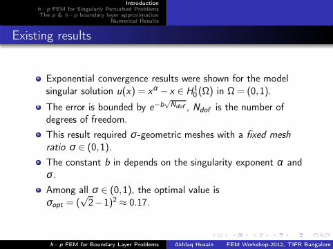
Exponential convergence results were shown for the modelsingular solution u(x) = xα − x ∈ H1

0 (Ω) in Ω = (0,1).

The error is bounded by e−b√

Ndof , Ndof is the number ofdegrees of freedom.

This result required σ -geometric meshes with a fixed mesh

ratio σ ∈ (0,1).

The constant b in depends on the singularity exponent α andσ .

Among all σ ∈ (0,1), the optimal value isσopt = (

√2−1)2 ≈ 0.17.



Numerical Results

Existing results

Babuška and Guo (1986-88) obtained exponential convergence

(an upper bound Ce−b 3√

Ndof ) on the error for 2D ellipticproblems polygonal domains in a series of landmark papers.

Key ingredients were geometric mesh refinements towards thecorners and nonuniform elemental polynomial degrees whichincrease linearly with the elements’ distance from corners.

The proofs of elliptic regularity results in terms of countablynormed spaces (an essential component of the exponentialconvergence proof) has been a major achievement.



Numerical Results

Existing results

Extension of the analytic regularity and the hp-convergenceanalysis of two dimensional problems to three dimensions wereundertaken by Babuška (1995-97).

hp-version of discontinuous Galerkin finite element method(hp-DGFEM) for elliptic problems on polyhedral domains hasbeen analyzed by D. Schotzau et al. (2009).

The method is shown to be exponentially accurate.



Numerical Results

Singularly Perturbed Problems : Introduction

Many partial differential equations in practical application areparameter-dependent and are of singularly perturbed type forsmall values of the parameter.



Numerical Results

Applications

Singularly perturbed problems find applications in1 Convection-diffusion equations.2 Plate and shell models for small thickness (Solid Mechanics).3 Navier-Stokes equations (Fluid Flow) having small viscosity

coefficients.4 Semi-conductor device modelling.



Numerical Results

Motivation

Most existing numerical methods employed for SPPs are loworder methods.

Boundary layers arise as solution components in singularlyperturbed elliptic boundary value problems.

Starting from early 90ties serious efforts have been made forresolution of boundary layers.

Approximation theory and convergence results for singularlyperturbed problems on smooth domains have been wellestablished within the framework of FDM and FEM.



Numerical Results

Motivation

The h−p version of the FEM for singularly perturbedboundary value problems on smooth and non-smooth domainshas been analyzed by Xenophontos (1996-98).

J. Melenk (2002) presented a complete analysis of a highorder (h−p) Finite Element Method (FEM), for a class ofSPPs on curvilinear polygons.

Obtained exponential convergence results.



Numerical Results

Boundary Layer Functions

Boundary Layer Function

A boundary layer functions is a function of the form

u(x) = exp

(−x

ε

)

, 0 < x < L, (1)

ε ∈ (0,1] is a small parameter that can approach zero.

L ≥ 1 is a length scale.

We look for convergence estimates that are robust, i.e.,uniform in ε , when (1) is approximated by piecewisepolynomials via h−p FEM.



Numerical Results

Boundary Layer Functions

Boundary layers (1) arise as solution components in singularlyperturbed elliptic boundary value problems, for example,

Singularly Perturbed Elliptic BVP

Lεuε := −ε2u′′ε (x)+uε (x) = f (x) on Ω = (−1,1) (2)

with the boundary conditions u(1) = u(−1) = 0. Here f ∈ L2 is agiven function.



Numerical Results

Variational Formulation


The variational formulation of the model problem (2) reads : Finduε ∈ H1

0 (Ω) such that

Bε(u,v) = F (v) ∀v ∈ H10 (Ω). (3)

Here

Bε(u,v) =

∫

Ω

(

ε2u′v ′ +uv)

dx

F (v) =

∫

Ωf (x)vdx .



Numerical Results


The bilinear form Bε(u,v) is coercive on H10 (Ω) in the energy

norm||uε || = (Bε (u,u))1/2.

Hence for every f ∈ L2, (5) admits a unique solution.

If f ∈ Hm(Ω), then uε ∈ Hm+2(Ω)∩H10 (Ω).

This regularity is non-uniform in ε since in the a priori shiftestimate

||uε ||Hm+2(Ω) ≤ C (m,ε)||f ||Hm(Ω)

the constant C depends on ε .



Numerical Results

Decomposition of the Solution

The following theorem presents a decomposition of uε into asmooth part uM

ε (x) and boundary layers

uε = exp

(−(1+ x)

ε

)

, uε = exp

(−(1− x)

ε

)

.

Decomposition Theorem

Theorem : Let f ∈ C∞(Ω). Then for every M ∈ N

u(x) = uMasm(x)+AMuM

ε +BM uMε (4)

where |AM |+ |BM |+ ||uMaym||l ≤ C (M, f ) for l = 0,1, · · · ,M.



Numerical Results

Finite Element Approximation

We obtain approximate solutions by restricting the variationalformulation to finite-dimensional subspaces.

Let ∆ = −l = x0 < x1 < x2 < · · · < xm = 1 be a mesh in[−1,1].

Set Ωj = (xj−1,xj),hj = xj − xj −1 for j = 1, · · · ,m.

Let p = (p(1), · · · ,p(m)),p(j) ≥ 1, denote a polynomial degreevector.

Define

Sp(∆) =

u ∈ C 0(Ω) : u|Ωj∈ ∏

pj

(Ωj), j = 1, · · · ,m

.

Sp0 (∆) = Sp(∆)∩u : u(±1) = 0.



Numerical Results

Finite Element Approximation

Clearly, Sp0 (∆) ⊂ H1

0 (Ω).

FEM Formulation

The FEM formulation of the model problem (2) reads : FinduFE ∈ S

p0 (∆) such that

Bε(uFE ,v) = F (v) ∀v ∈ S

p0 . (5)

The finite element solution uFE is quasi-optimal, i.e.

||u−uFE ||ε ≤ ||u− v ||ε for all v ∈ Sp0 (∆).



Numerical Results

The p & h−p boundary layer approximation

Approximation on a Single element

Theorem : Let uλ ,ε = exp(

−λ(1+x)ε

)

, x ∈ (−1,1), ε > 0,

λ = a+ ib, a2 +b2 = 1. Then for every p ≥ 1, there existsQp ∈ ∏p(Ω) such that

Qp(±1) = uλ ,ε (±1), (6)

||u′λ ,ε −Q ′

p||2L2(Ω) ≤ Cε−1

(

e

(2p +1)ε

)2p+1

, (7)

||uλ ,ε −Qp||2L2(Ω) ≤ Cεp−1

(

e

(2p +1)ε

)2p+1

. (8)



Numerical Results


Proof : Using results from Babuška and B.A. Szabo(Lecture notes on finite element analysis) it follows thatthere exists Qp ∈ ∏p(Ω) satisfying Qp(±1) = uλ ,ε (±1) and

||u′λ ,ε −Q ′

p||2L2(Ω) ≤1

(2p)!|u′

λ ,ε |2V p(Ω) (9)

and

||uλ ,ε −Qp||2L2(Ω) ≤1

p(p +1)(2p−1)!|u′

λ ,ε |2V p−1(Ω). (10)

where

|u′|2V q(Ω) =∫ 1

−1(1−ξ 2)q|u(q+1)(x)|2dx .



Numerical Results


Stirling’s formula yields

1

(2q)!≤ C

(

e

2q +1

)2q+1/2

. (12)

where C is independent of q. Combining (9-12), we get (7)and (8).

Estimates (7) and (8) imply super-exponential convergence asp → ∞, provided

p := p +1

2>

e

2ε. (13)



Numerical Results


For small values of ε , (13) will only be satisfied forunrealistically high values of p.

We now consider an h−p approximation result, where themesh changes at each step that p is increased.

Only the relative size, and not the number of elements need tobe altered to achieve exponential convergence

Precisely this is an rp version.



Numerical Results


h−p version approximation

Theorem : Let uλ ,ε be as in the previous Theorem. Let, (∆, p) besuch that for some κ independent of p,ε satisfying0 < κ0 ≤ κ < 4/ε ,

p = p,1 ∆ = −1,−1+ κ pε ,1 if kpε < 2.

p = p ∆ = −1,1 if kpε ≥ 2.

Then there exists up ∈ S p(∆) satisfying up(±1) = uε ,λ (±1) and

||uλ ,ε −up||ε ≤ Cε1/2qp ,

||uλ ,ε −up||0 ≤ Cε1/2qp ,

||uλ ,ε −up||1 ≤ Cε−1/2qp.



Numerical Results


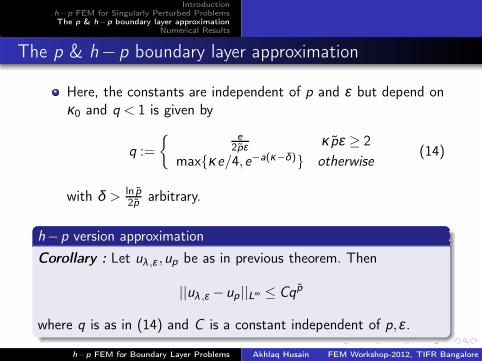
Here, the constants are independent of p and ε but depend onκ0 and q < 1 is given by

q :=

e2pε κ pε ≥ 2

maxκe/4,e−a(κ−δ) otherwise(14)

with δ > ln p2p arbitrary.

h−p version approximation

Corollary : Let uλ ,ε ,up be as in previous theorem. Then

||uλ ,ε −up||L∞ ≤ Cqp

where q is as in (14) and C is a constant independent of p,ε .



Numerical Results


Proof : Follows from the interpolation inequality

||u||L∞(Ω) ≤ 2||u||1/20 ||u′||1/2

0

and the previous theorem.



Numerical Results

Numerical Results

Consider the model problem (5) with

f (x) =x +1

2.

This problem was also considered by Canuto (1988) havingexact solution

u(x) =sinh

(

x+1ε

)

sinh(

2ε) − x +1

2.

Evidently, it has only one boundary layer near x = 1, i.e.AM = 0 in (4).

The relative error in the energy norm is given by

ER(ε) =||u−uFE ||ε

||u||εh−p FEM for Boundary Layer Problems Akhlaq Husain FEM Workshop-2012, TIFR Bangalore


Numerical Results

Numerical Results

We depict ER(ε) versus the number of degrees of freedom inthe finite element method.

We compare four finite element methods :

(a) the p version with one element,(b) the h version with p = 1,(c) the h−p version with 2 elements with κ = 1 and(d) the h version (taking p = 1) with the exponential mesh∆ = −1,x1, · · · ,xm−1,1, where for m even

xi :=

−1 i = 0−ε p ln

(

1− c i−1

m−1

)

i = 1, · · · ,m (15)

with c = 1− exp(−1/(dp)).



Numerical Results

Numerical Results

The mesh (15) was obtained by Schwab and Xenophontos(1996).

It is known that for h version with p = 1, the error obtainedwith this mesh is optimal as m → ∞.

Figures 1, 2 and 3 show the performance of the four methodsfor ε = 10−2, ε = 10−4 and ε = 10−8, respectively.



Numerical Results

Numerical Results



Numerical Results

Summary

The rate of convergence of the uniform h version is O(N−1/2)while

The uniform rate (in ε) for the p version on a single element isO(N−1)

For the h version with exponential mesh, the optimal algebraicrate of O(N−1) is observed.

The h−p version shows exponential rate as expected.



Numerical Results

Summary

The errors for the h version with exponential mesh and theh−p version both decrease as ε becomes smaller, at the rateof O(ε1/2).

The other two version does not display this decrease as ε → 0.

For a fixed number of degrees of freedom, the error with theh−p version is seen to be consistently the smallest of the fourmethods.

Thus h−p version is extremely robust and efficient even forvery small values of ε relative energy errors of 10−8 werereached with only N = 15 degrees of freedom.



Numerical Results

R.A. Adams (1975) : Sobolev Spaces, Academic Press, New York.

I. Babuška and B. Guo (1996) : Approximation peroperties of the h−p versionof the finite element method, Comp. Methods Appl. Mech. Engrg, 133, 319-346.

I. Babuška and B.A. Szabo, Lecture notes on finite element analysis.

C. Canuto, Spectral methods and a maximum principle, Math. Comp. 51 (1988),615-629.

J. M. Melenk, hp Finite element methdos for singular perturbations, ETH Zurich,(2002).

K. W. Morton, Numerical Solution of Convection-Diffusion Problems, Chapmanand Hall, (1996).

C. Schwab, M. Suri, Boundary layers approximation by spectral/hp methods,International Congress of Spectral and Higer Order Methods, ICOSAHOM-1995,(1995).

C. Schwab, M. Suri, The p and h-p versions of the finite element method forproblems with boundary layers, Math. Comp., 65, 1403-1429, (1996).

C. Schwab, M. Suri, C. Xenophontos, The hp finite element method for problemsin mechanics with boundary layers, Comput. Meth. Appl. Mech. Eng., 157,311-333, (1996).



Numerical Results

Ch. Schwab, p and h−p Finite element methods, Clarendon Press, Oxford,(1998).

C. Schwab, J.M. Melenk, hp FEM for reaction-diffusion equations I : robustexponential convergence, SIAM J. Numer. Anal., 35, 1520-1557, (1998).

S.K. Tomar, h−p Spectral element methods for elliptic problems overnon-smooth domains using parallel computers, Computing 78, 117-143, (2006).

C. Xenophontos, The h-p finite element method for singularly perturbedboundary value problems on smooth domains, Doctoral Dissertation, Universityof Maryland Baltimore County, 1996.

C. Xenophontos, The h-p finite element method for singularly perturbedboundary value problems on smooth domains, Math. Models and Methods inApplied Sciences, Vol. 8, 69-79 (1998).

C. Xenophontos, The h-p finite element method for singularly perturbedproblems on non-smooth domains, Numerical Methods for Partial DiffernetialEquations, Vol. 16, 1-28 (1998).


h p finite element methods for boundary layer...

Documents