Haar Graph Pooling

Yu Guang Wang 1 Ming Li 2 Zheng Ma 3 Guido Montufar 4 5 Xiaosheng Zhuang 5 Yanan Fan 1

Abstract

Deep Graph Neural Networks (GNNs) are usefulmodels for graph classification and graph-basedregression tasks. In these tasks, graph pooling is acritical ingredient by which GNNs adapt to inputgraphs of varying size and structure. We proposea new graph pooling operation based on compres-sive Haar transforms — HaarPooling. HaarPool-ing implements a cascade of pooling operations;it is computed by following a sequence of clus-terings of the input graph. A HaarPooling layertransforms a given input graph to an output graphwith a smaller node number and the same featuredimension; the compressive Haar transform filtersout fine detail information in the Haar waveletdomain. In this way, all the HaarPooling layerstogether synthesize the features of any given inputgraph into a feature vector of uniform size. Suchtransforms provide a sparse characterization of thedata and preserve the structure information of theinput graph. GNNs implemented with standardgraph convolution layers and HaarPooling layersachieve state of the art performance on diversegraph classification and regression problems.

1. IntroductionGraph Neural Networks (GNNs) have demonstrated excel-lent performance in node classification tasks and are verypromising in graph classification and regression (Bronsteinet al., 2017; Battaglia et al., 2018; Zhang et al., 2018b; Zhouet al., 2018; Wu et al., 2019). In node classification, theinput is a single graph with missing node labels that are to

*First Four Authors have equal contribution. 1School of Math-ematics and Statistics, University of New South Wales, Sydney,Australia 2School of Teacher Education, Zhejiang Normal Uni-versity, Jinhua, China 3Department of Physics, Princeton Uni-versity, New Jersey, USA 4Max Planck Institute for Mathemat-ics in the Sciences, Leipzig, Germany 5Department of Math-ematics, City University of Hong Kong, Hong Kong. Corre-spondence to: Yu Guang Wang <yuguang.wang@unsw.edu.au>,Ming Li <ming.li.ltu@gmail.com>, Guido Montufar <montu-far@math.ucla.edu>.

be predicted from the known node labels. In this problem,GNNs with appropriate graph convolutions can be trainedbased on a single input graph, and achieve state-of-the-artperformance (Defferrard et al., 2016; Kipf & Welling, 2017;Ma et al., 2019b). Different from node classification, graphclassification is a task where the label of any given graph-structured sample is to be predicted based on a training setof labeled graph-structured samples. This is similar to theimage classification task tackled by traditional deep convo-lutional neural networks. The significant difference is thathere each input sample may have an arbitrary adjacencystructure instead of the fixed, regular grids that are used instandard pixel images. This raises two crucial challenges:1) How can GNNs exploit the graph structure informationof the input data? 2) How can GNNs handle input graphswith varying number of nodes and connectivity structures?

These problems have motivated the design of proper graphconvolution and graph pooling to allow GNNs to capturethe geometric information of each data sample (Zhang et al.,2018a; Ying et al., 2018; Cangea et al., 2018; Gao & Ji,2019; Knyazev et al., 2019; Ma et al., 2019a; Lee et al.,2019). Graph convolution plays an important role, espe-cially in question 1).

The following is a widely utilized type of graph convolutionlayer, proposed by (Kipf & Welling, 2017):

Xout = AX inW. (1)

Here A = D−1/2(A+ I)D−1/2 ∈ RN×N is a normalizedversion of the adjacency matrix A of the input graph, whereI is the identity matrix and D is the degree matrix for A+ I .Further, X in ∈ RN×d is the array of d-dimensional featureson the N nodes of the graph, and W ∈ Rd×m is the filterparameter matrix. We call the graph convolution of Kipf &Welling (2017) in Equation (1) the GCN convolution.

The graph convolution in Equation (1) captures the struc-tural information of the input in terms of A (or A), and Wtransforms the feature dimension from d to m. As the filtersize d × m is independent of the graph size, it allows afixed network architecture to process input graphs of vary-ing sizes. The GCN convolution preserves the number ofnodes, and hence the output dimension of the network isnot unique. Graph pooling provides an effective way toovercome this obstacle. Some existing approaches, Eigen-

arX

iv:1

909.

1158

0v2

[cs

.LG

] 9

Feb

202

0

Haar Graph Pooling

Pooling (Ma et al., 2019a), for example, incorporate bothfeatures and graph structure, which gives very good perfor-mance on graph classification.

In this paper, we propose a new graph pooling strategybased on a sparse Haar representation of the data, whichwe call Haar Graph Pooling, or simply HaarPooling. Itis built on the Haar basis (Wang & Zhuang, 2019; 2020;Li et al., 2019), which is a localized wavelet-like basis ona graph. We define HaarPooling by the compressive Haartransform of the graph data, which is a nonlinear transformthat operates in the Haar wavelet domain by using the Haarbasis. For an input data sample, which consists of a graph Gand the feature on the nodes X in ∈ RN×d, the compressiveHaar transform is determined by the Haar basis vectors onG and maps X in into a matrix Xout of dimension d×N1.The pooled feature Xout is in the Haar wavelet domain andextracts the coarser feature of the input. Thus, HaarPoolingcan provide sparse representations of graph data that distillstructural graph information.

The Haar basis and its compressive transform can be usedto define cascading pooling layers, i.e., for each layer, wedefine an orthonormal Haar basis and its compressive Haartransform. Each HaarPooling layer pools the graph inputfrom the previous layer to output with a smaller node num-ber and the same feature dimension. In this way, all theHaarPooling layers together synthesize the features of allgraph input samples into feature vectors with the same size.We then obtain an output of a fixed dimension, regardlessof the size of the input.

The algorithm of HaarPooling is simple to implement asthe Haar basis and the compressive Haar transforms canbe computed by the explicit formula. The computation ofHaarPooling is cheap, with nearly linear time complexity.HaarPooling can connect to any graph convolution. TheGNNs with HaarPooling can handle multiple tasks. Exper-iments in Section 5 demonstrate that the GNN with Haar-Pooling achieves state of the art performance on variousgraph classification and regression tasks.

2. Related WorkGraph pooling is a vital step when building a GNN model forgraph classification and regression, as one needs a unifiedgraph-level rather than node-level representation for graph-structured inputs of which size and topology are changing.The most direct pooling method, as provided by the graphconvolutional layer (Duvenaud et al., 2015), takes the globalmean and sum of the features of the nodes as a simplegraph-level representation. This pooling operation treatsall the nodes equally and uses the global geometry of thegraph. ChebNet (Defferrard et al., 2016) used a graph coars-ening procedure to build the pooling module, for which

one needs a graph clustering algorithm to obtain subgraphs.One drawback of this topology-based strategy is that it doesnot combine the node features in the pooling. The globalpooling method considers the information about node em-beddings, which can achieve the entire graph representa-tion. As a general framework for graph classification andregression problems, MPNN (Gilmer et al., 2017) used theSet2Set method (Vinyals et al., 2015) that would obtain agraph-level representation of the graph input samples. TheSortPool (Zhang et al., 2018a) proposed a method that couldrank and select the nodes by sorting their feature representa-tion and then feed them into a traditional 1-D convolutionalor dense layer. These global pooling methods did not utilizethe hierarchical structure of the graph, which may carryuseful geometric information of data.

One notable recent argument is to build a differentiable anddata-dependent pooling layer with learnable operations orparameters, which has brought a substantial improvement ingraph classification tasks. The DiffPool (Ying et al., 2018)proposed a differentiable pooling layer that learns a clusterassignment matrix over the nodes relating to the output ofa GNN model. One difficulty of DiffPool is its vast stor-age complexity, which is due to the computation of the softclustering. The TopKPooling (Cangea et al., 2018; Gao &Ji, 2019; Knyazev et al., 2019) proposed a pooling methodthat samples a subset of essential nodes by manipulating atrainable projection vector. The Self-Attention Graph Pool-ing (SAGPool) (Lee et al., 2019) proposed an analogouspooling that applied the GCN module to compute the nodescores instead of the projection vector in the TopKPooling.These hierarchical pooling methods technically still em-ploy mean/max pooling procedures to aggregate the featurerepresentation of super-nodes. To preserve more edge infor-mation of the graph, EdgePool (Diehl et al., 2019) proposedto incorporate edge contraction. The StructPool (Yuan & Ji,2020) proposed a graph pooling that employed conditionalrandom fields to represent the relation of different nodes.

The spectral-based pooling method suggests another design,which operates the graph pooling in the frequency domain,for example, the Fourier domain or the wavelet domain.By its nature, the spectral-based approach can combinethe graph structure and the node features. The LaplacianPooling (LaPool) (Noutahi et al., 2019) proposed a pool-ing method that dynamically selected the centroid nodesand their corresponding follower nodes by using a graphLaplacian-based attention mechanism. EigenPool (Ma et al.,2019a) introduced a graph pooling that used the local graphFourier transform to extract subgraph information. Its poten-tial drawback lies in the inherent computing bottleneck forthe Laplacian-based graph Fourier transform, given the highcomputational cost for the eigendecomposition of the graphLaplacian. Our HaarPooling is a spectral-based method thatapplies the Haar basis system in the node feature represen-

Haar Graph Pooling

tation, as we now introduce.

3. Haar Graph PoolingIn this section, we give an overview of the proposed Haar-Pooling framework. First we define the pooling architecturein terms of a coarse-grained chain, i.e., a sequence of graphs(G0,G1, . . . ,GK), where the nodes of the (j + 1)th graphGj+1 correspond to the clusters of nodes of the jth graph Gjfor each j = 0, . . . ,K−1. Based on the chain, we constructthe Haar basis and the compressive Haar transform. Thelatter then defines the HaarPooling operation. Each layerin the chain determines which sets of nodes the networkpools, and the compressive Haar transform synthesizes theinformation from the graph and node feature for pooling.

Chain of coarse-grained graphs for pooling Graphpooling amounts to defining a sequence of coarse-grainedgraphs. In our chain, each graph is an induced graph thatarises from grouping (clustering) certain subsets of nodesfrom the previous graph. We use clustering algorithms togenerate the groupings of nodes. There are many good can-didates, such as spectral clustering (Shi & Malik, 2000),k-means clustering (Pakhira, 2014), DBSCAN (Ester et al.,1996), OPTICS (Ankerst et al., 1999) and METIS (Karypis& Kumar, 1998). Any of these will work with HaarPooling.Figure 1 shows an example of a chain with 3 levels, for aninput graph G0.

a b c d e f g h G0

a b c d e f g h G1

a b c d e f g h G2

Figure 1. A coarse-grained chain of graphs. The input has 8 nodes;the second and top levels have 3 and single nodes.

Compressive Haar transforms on chain For each layerof the chain, we will have a feature representation. We de-fine these in terms of the Haar basis. The Haar basis repre-sents graph-structured data by low- and high-frequency Haarcoefficients in the frequency domain. The low-frequencycoefficients contain the coarse information of the originaldata, while the high-frequency coefficients contain the finedetails. In HaarPooing, the data is pooled (or compressed)by discarding the fine detail information.

The Haar basis can be compressed in each layer. Consider achain. The two subsequent graphs haveNj+1 andNj nodes,Nj+1 < Nj . We selectNj elements from the (j+1)th layer

for the jth layer, each of which is a vector of size Nj+1.These Nj vectors form a matrix Φj of size Nj+1 ×Nj . Wecall Φj the compressive Haar basis matrix for this particularjth layer. This then defines the compressive Haar transformΦT

j Xin for feature X in of size Nj × d.

Computational strategy of HaarPooling By compres-sive Haar transform, we can define the HaarPooling.

Definition 1 (HaarPooling). The HaarPooling for a graphneural network with K pooling layers is defined as

Xoutj = ΦT

j Xinj , j = 0, 1, . . . ,K − 1,

where Φj is the Nj ×Nj+1 compressive Haar basis matrixfor the jth layer, X in

j ∈ RNj×dj is the input feature array,and Xout

j ∈ RNj+1×dj is the output feature array, for someNj > Nj+1, j = 0, 1, . . . ,K − 1, and NK = 1. For eachj, the corresponding layer is called the jth HaarPoolinglayer. More explicitly, we also write Φj as Φ

(j)Nj×Nj+1

.

HaarPooling has the following fundamental properties.

• First, the HaarPooling is a hierarchically structured al-gorithm. The coarse-grained chain determines the hier-archical relation in different HaarPooling layers. Thenode number of each HaarPooling layer is equal to thenumber of nodes of the subgraph of the correspondinglayer of the chain. As the top-level of the chain can haveone node, the HaarPooling finally reduces the number ofnodes to one, thus producing a fixed dimensional outputin the last HaarPooling layer.

• The HaarPooling uses the sparse Haar representation onchain structure. In each HaarPooling layer, the repre-sentation then combines the features of input X in

j withthe geometric information of the graphs of the jth and(j + 1)th layers of the chain.

• By the property of the Haar basis, the HaarPooling onlydrops the high-frequency information of the input data.The Xout

j mirrors the low-frequency information in theHaar wavelet representation of X in

j . Thus, HaarPoolingpreserves the essential information of the graph input,and the network has small information loss in pooling.

Example Figure 2 shows the computational details of theHaarPooling associated with the chain from Figure 1. Thereare two HaarPooling layers. In the first layer, the inputX in

1 of size 8× d1 is transformed by the compressive Haarbasis matrix Φ

(0)8×3 which consists of the first three column

vectors of the full Haar basis Φ(0)8×8 in (a), and the output is

a 3 × d1 matrix Xout1 . In the second layer, the input X in

2

of size 3 × d2 (usually Xout1 followed by convolution) is

Haar Graph Pooling

(a) First HaarPooling Layer for G0 → G1. (b) Second HaarPooling Layer for G1 → G2.

Figure 2. Computational strategy of HaarPooling. We use the chain in Figure 1, and then the network has two HaarPooling layers:G0 → G1 and G1 → G2. The input of each layer is pooled by the compressive Haar transform for that layer: in the first layer, the inputX in

1 = (xi,j) ∈ R8×d1 is transformed by the compressive Haar basis matrix Φ(0)8×3 of size 8× 3 formed by the first three column vectors

of the original Haar basis, and the output is a feature array of size 3× d1; in the second layer, X in2 = (yi,j) ∈ R3×d2 is transformed by

the first column vector Φ(1)3×1 and the output is a feature vector of size 1× d2. In the plots of the Haar basis matrix, the colors indicate the

value of the entries of the Haar basis matrix.

transformed by the compressive Haar matrix Φ(1)3×1, which is

the first column vector of the full Haar basis matrix Φ(1)3×3 in

(b). By the construction of the Haar basis in relation to thechain (see Section 4), each of the first three column vectorsφ(0)1 , φ

(0)2 and φ(0)3 of Φ

(0)8×3 has only up to three different

values. This bound is precisely the number of nodes of G1.For each column of φ(0)` , all nodes with the same parent takethe same value. Similarly, the 3× 1 vector φ(1)1 is constant.This example shows that the HaarPooling amalgamates thenode feature by adding the same weight to the nodes thatare in the same cluster of the coarser layer, and in this way,pools the feature using the graph clustering information.

4. Compressive Haar TransformsChain of graphs by clustering For a graph G =(V,E,w), where V,E,w are the vertices, edges, andweights on edges, a graph Gcg = (V cg, Ecg, wcg) is acoarse-grained graph of G if |V cg| ≤ |V | and each nodeof G has only one parent node in Gcg associated with it.Each node of Gcg is called a cluster of G. For integersJ > 0, a coarse-grained chain for G is a sequence of graphsG0→J := (G0,G1, . . . ,GJ) with G0 = G and such that Gj+1

is a coarse-grained graph of Gj for each j = 0, 1, . . . , J −1,and GJ has only one node. Here, we call the graph GJ thetop level or the coarsest level and G0 the bottom level or thefinest level. The chain G0→J hierarchically coarsens graphG. We use the notation J + 1 for the number of layers ofthe chain, to distinguish it from the number K of layers forpooling. For details about graphs and chains, we refer thereader to the examples by (Chung & Graham, 1997; Ham-mond et al., 2011; Chui et al., 2015; 2018; Wang & Zhuang,

2019; 2020).

Haar (1910) first introduced Haar basis on the real axis.It is a particular example of the more general Daubechieswavelets (Daubechies, 1992). Haar basis was later con-structed on graphs by (Belkin et al., 2006), and also (Chuiet al., 2015; Wang & Zhuang, 2019; 2020; Li et al., 2019).

Construction of Haar basis The Haar bases {φ(j)` }Nj

`=1,j = 0, . . . , J , is a sequence of collections of vectors. EachHaar basis is associated with a single layer of the chainG0→J of a graph G. For j = 0, . . . , J , we let the matrixΦj = (φ

(j)1 , . . . , φ

(j)Nj

) ∈ RNj×Nj and call the matrix Φj

Haar transform matrix for the jth layer. In the following, wedetail the construction of the Haar basis based on the coarse-grained chain of a graph, as discussed in (Wang & Zhuang,2019; 2020; Li et al., 2019). We attach the algorithmicpseudo-codes for generating the Haar basis on the graph inthe supplementary material.

Step 1. Let Gcg = (V cg, Ecg, wcg) be a coarse-grainedgraph of G = (V,E,w) with N cg := |V cg|. Here weuse the sub-index “cg” to indicate the symbol is for thecoarse-grained graph. Each vertex vcg ∈ V cg is a clustervcg = {v ∈ V | v has parent vcg} of G. Order V cg, e.g.,by degrees of vertices or weights of vertices, as V cg ={vcg1 , . . . , vcgNcg}. We define N cg vectors φcg` on Gcg by

φcg1 (vcg) :=1√N cg

, vcg ∈ V cg, (2)

and for ` = 2, . . . , N cg,

φcg` :=

√N cg − `+ 1

N cg − `+ 2

(χcg`−1 −

∑Ncg

j=` χcgj

N cg − `+ 1

), (3)

Haar Graph Pooling

where χcgj is the indicator function for the jth vertex vcgj ∈

V cg on G given by

χcgj (vcg) :=

{1, vcg = vcgj ,

0, vcg ∈ V cg\{vcgj }.

Then, the {φcg` }Ncg

`=1 forms an orthonormal basis for l2(Gcg).Each v ∈ V belongs to exactly one cluster vcg ∈ V cg. Inview of this, for each ` = 1, . . . , N cg, we can extend thevector φcg` on Gcg to a vector φ`,1 on G by

φ`,1(v) :=φcg` (vcg)√|vcg|

, v ∈ vcg,

here |vcg| := k` is the size of the cluster vcg, i.e., the numberof vertices in G whose common parent is vcg. We order thecluster vcg` , e.g., by degrees of vertices, as

vcg` = {v`,1, . . . , v`,k`} ⊆ V.

For k = 2, . . . , k`, similar to Equation (3), define

φ`,k =

√k` − k + 1

k` − k + 2

(χ`,k−1 −

∑k`

j=k χ`,j

k` − k + 1

),

where for j = 1, . . . , k`, χ`,j is given by

χ`,j(v) :=

{1, v = v`,j ,

0, v ∈ V \{v`,j}.

Then, the resulting {φ`,k : ` = 1, . . . , N cg, k = 1, . . . , k`}is an orthonormal basis for l2(G).

Step 2. Let G0→J be a coarse-grained chain for the graph G.An orthonormal basis {φ(J)` }NJ

`=1 for l2(GJ) is generated us-ing Equations (2) and (3). We then repeatedly use Step 1: forj = 0, . . . , J − 1, generate an orthonormal basis {φ(j)` }

Nj

`=1

for l2(Gj) from the orthonormal basis {φ(j+1)` }Nj+1

`=1 for thecoarse-grained graph Gj+1 that was derived in the previoussteps. We call the sequence {φ` := φ

(0)` }N0

`=1 of vectors atthe finest level, the Haar global orthonormal basis, or sim-ply the Haar basis, for G associated with the chain G0→J .The orthonormal basis {φ(j)` }

Nj

`=1 for l2(Gj), j = 1, . . . , Jis called the Haar basis for the jth layer.

Compressive Haar basis Suppose we have constructedthe (full) Haar basis {φ(j)` }

Nj

`=0 for each layer Gj of thechain G0→K . The compressive Haar basis for layer j is{φ(j)` }

Nj+1

`=0 . We will use the transforms of this basis todefine HaarPooling.

Orthogonality For each level j = 0, . . . , J , the sequence{φ(j)` }

Nj

`=1, with Nj := |Vj |, is an orthonormal basis for thespace l2(Gj) of square-summable sequences on the graphGj , so that (φ

(j)` )Tφ

(j)`′ = δ`,`′ . For each j, {φ(j)` }

Nj

`=1 is theHaar basis system for the chain Gj→J .

Locality Let G0→J be a coarse-grained chain for G. Ifeach parent of level Gj , j = 1, . . . , J , contains at leasttwo children, the number of different scalar values of thecomponents of the Haar basis vector φ(j)` , ` = 1, . . . , Nj , isbounded by a constant independent of j.

In Figure 2, the Haar basis is generated based on the coarse-grained chain G0→2 := (G0,G1,G2), where G0,G1,G2 aregraphs with 8, 3, 1 nodes. The two colorful matrices showthe two Haar bases for the layers 0 and 1 in the chain G0→2.There are in total 8 vectors of the Haar basis for G0 eachwith length 8, and 3 vectors of the Haar basis for G1 eachwith length 3. Haar basis matrix for each level of the chainhas up to 3 different values in each column, as indicatedby colors in each matrix. For j = 0, 1, each node of Gj isa cluster of nodes in Gj+1. Each column of the matrix isa member of the Haar basis on the individual layer of thechain. The first three column vectors of Φ1 can be reducedto an orthonormal basis of G1 and the first column vector ofG1 to the constant basis for G2. This connection ensures thatthe compressive Haar transforms for HaarPooling is alsocomputationally feasible.

Adjoint and forward Haar transforms We utilize ad-joint and forward Haar transforms to compute HaarPooling.Due to the sparsity of the Haar basis matrix, the transformsare computationally feasible. The adjoint Haar transformfor the signal f on Gj is

(Φj)T f =

(∑v∈V

φ(j)1 (v)f(v), . . . ,

∑v∈V

φ(j)Nj

(v)f(v)

)∈ RNj ,

(4)and the forward Haar transform for (coefficients) vectorc := (c1, . . . , cNj

) ∈ RNj is

(Φjc)(v) =

Nj∑`=1

φ(j)` (v)c`, v ∈ Vj . (5)

We call the components of (Φj)T f the Haar (wavelet) co-

efficients for f . The adjoint Haar transform represents thesignal in the Haar wavelet domain by computing the Haarcoefficients for graph signal, and the forward transformsends back the Haar coefficients to the time domain. Here,the adjoint and forward Haar transforms can be extended toa feature data with size Nj × dj by replacing the columnvector f with the feature array.Proposition 2. The adjoint and forward Haar Transformsare invertible in that for j = 0, . . . , J and vector f on graphGj ,

f = Φj(Φj)T f.

Proposition 2 shows that the forward Haar transform canrecover the graph signal f from the adjoint Haar transform(Φj)

T f , which means that adjoint and forward Haar trans-forms have zero-loss in graph signal transmission.

Haar Graph Pooling

Compressive Haar transforms Now for a graph neuralnetwork, suppose we want to use K pooling layers forK ≥ 1. We associate the chain G0→K of an input graphwith the pooling by linking the jth layer of pooling withthe jth layer of the chain. Then, we can use the Haar basissystem on the chain to define the pooling operation. Bythe property of Haar basis, in the Haar transforms for layerj, 0 ≤ j ≤ K − 1, of the Nj Haar coefficients, the firstNj+1 coefficients are the low-frequency coefficients, whichreflect the approximation to the original data, and the re-maining (Nj − Nj+1) coefficients are in high frequency,which contains fine details of the Haar wavelet decompo-sition. To define pooling, we remove the high-frequencycoefficients in the Haar wavelet representation and then ob-tain the compressive Haar transforms for the feature X in

j atlayers j = 0, . . . ,K − 1, which then gives the HaarPoolingin Definition 1.

As shown in the following formula, the compressive Haartransform incorporates the neighborhood information of thegraph signal as compared to the full Haar transform. Thus,the HaarPooling can take the average information of thedata f over nodes in the same cluster.∥∥ΦT

j Xinj

∥∥2 =∑

p∈Gj+1

1

|Pa(v)|∣∣∣ ∑p=Pa(v)

X inj (v)

∣∣∣2∥∥∥ΦT

j Xinj

∥∥∥2 =∑

p∈Gj+1

∑p=Pa(v)

∣∣∣X inj (v)

∣∣∣2, (6)

where Φj is the full Haar basis matrix at the jth layer and|PaG(v)| is the number of nodes in the cluster which thenode v lies in. Here, 1/

√|PaG(v)| can be taken out of

summation as Pa(v) is in fact a set of nodes. We show thederivation of formula in Equation (6) in the supplementary.

In HaarPooling, the compression or pooling occurs in theHaar wavelet domain. It transforms the features on thenodes to the Haar wavelet domain. It then discards the high-frequency coefficients in the sparse Haar wavelet represen-tation. See Figure 2 for a two-layer HaarPooling example.

5. ExperimentsIn this section, we present the test results of HaarPooling onvarious datasets in graph classification and regression tasks.We show a performance comparison of the HaarPoolingwith existing graph pooling methods. All the experimentsuse PyTorch Geometric (Fey & Lenssen, 2019) and wererun in Google Cloud using 4 Nvidia Telsa T4 with 2560CUDA cores, compute 7.5, 16GB GDDR6 VRAM.

5.1. HaarPooling on Classification Benchmarks

Datasets and baseline methods To verify whether theproposed framework can hierarchically learn good graph

representations for classification, we evaluate HaarPoolingon five widely used benchmark datasets for graph classifi-cation (Kersting et al., 2016), including one protein graphdataset PROTEINS (Borgwardt et al., 2005; Dobson &Doig, 2003); two mutagen datasets MUTAG (Debnath et al.,1991; Kriege & Mutzel, 2012) and MUTAGEN (Riesen &Bunke, 2008; Kazius et al., 2005) (full name Mutagenic-ity); and two datasets that consist of chemical compoundsscreened for activity against non-small cell lung cancer andovarian cancer cell lines, NCI1 and NCI109 (Wale et al.,2008). We include datasets from different domains, sam-ples, and graph sizes to give a comprehensive understandingof how the HaarPooling performs with datasets in variousscenarios. Table 1 summarizes some statistical informa-tion of the datasets: each dataset containing graphs withdifferent sizes and structures, the number of data samplesranges from 188 to 4,337, the average number of nodes isfrom 17.93 to 39.06, and the average number of edges isfrom 19.79 to 72.82. We compare HaarPool with SortPool(Zhang et al., 2018a), DiffPool (Ying et al., 2018), gPool(Gao & Ji, 2019), SAGPool (Lee et al., 2019), EigenPool(Ma et al., 2019a), CSM (Kriege & Mutzel, 2012) and GIN(Xu et al., 2019) on the above datasets.

Training In the experiment, we use a GNN with at most 3GCN (Kipf & Welling, 2017) convolutional layers plus oneHaarPooling layer, followed by three fully connected layers.The hyperparameters of the network are adjusted case bycase. We use spectral clustering to generate a chain with thenumber of layers given. Spectral clustering, which exploitsthe eigenvalues of the graph Laplacian, has proved excellentperformance in coarsening a variety of data patterns and canhandle isolated nodes.

We apply random shuffling for the dataset. We split thewhole dataset into the training, validation, and test sets withpercentages 80%, 10%, and 10%, respectively. We usethe Adam optimizer (Kingma & Ba, 2015), early stoppingcriterion, and patience, and give the specific values in thesupplementary. Here, the early stopping criterion was thatthe validation loss does not improve for 50 epochs, witha maximum of 150 epochs, as suggested by Shchur et al.(2018).

The architecture of GNN is identified by the layer type andthe number of hidden nodes at each layer. For example,we denote 3GC256-HP-2FC256-FC128 to represent a GNNarchitecture with 3 GCNConv layers, each with 256 hiddennodes, plus one HaarPooling layer followed by 2 fully con-nected layers, each with 256 hidden nodes, and by one fullyconnected layer with 128 hidden nodes. Table 3 shows theGNN architecture for each dataset.

Results Table 2 reports the classification test accuracy.GNNs with HaarPooling have excellent performance on all

Haar Graph Pooling

Table 1. Summary statistics of the graph classification datasets.Dataset MUTAG PROTEINS NCI1 NCI109 MUTAGEN

max #nodes 28 620 111 111 417min #nodes 10 4 3 4 4avg #nodes 17.93 39.06 29.87 29.68 30.32avg #edges 19.79 72.82 32.30 32.13 30.77#graphs 188 1,113 4,110 4,127 4,337#classes 2 2 2 2 2

Table 2. Performance comparison for graph classification tasks (test accuracy in percent, showingthe standard deviation over ten repetitions of the experiment).

Method MUTAG PROTEINS NCI1 NCI109 MUTAGEN

CSM 85.4 – – – –GIN 89.4 76.2 82.7 – –SortPool 85.8 75.5 74.4 72.3* 78.8*DiffPool – 76.3 76.0* 74.1* 80.6*gPool – 77.7 – – –SAGPool – 72.1 74.2 74.1 –EigenPool – 76.6 77.0 74.9 79.5

HaarPool (ours) 90.0±3.6 80.4±1.8 78.6±0.5 75.6±1.2 80.9±1.5

‘*’ indicates records retrieved from EigenPool (Ma et al., 2019a), ‘–’ means that there are no publicrecords for the method on the dataset, and bold font is used to highlight the best performance in the list.

datasets. In 4 out of 5 datasets, it achieves top accuracy. Itshows that HaarPooling, with an appropriate graph convo-lution, can achieve top performance on a variety of graphclassification tasks, and in some cases, improve state of theart by a few percentage points.

Table 3. Network architecture.

Dataset Layers and #Hidden Nodes

MUTAG GC60-HP-FC60-FC180-FC60PROTEINS 2GC128-HP-2GC128-HP-2GC128-

HP-GC128-2FC128-FC64NCI1 2GC256-HP-FC256-FC1024-FC2048NCI109 3GC256-HP-2FC256-FC128MUTAGEN 3GC256-HP-2FC256-FC128

5.2. HaarPooling on Triangles Classification

We test GNN with HaarPooling on the graph dataset Trian-gles (Knyazev et al., 2019). Triangles is a 10 class classifi-cation problem with 45,000 graphs. The average numbersof nodes and edges of the graphs are 20.85 and 32.74, re-spectively. In the experiment, the network utilizes GINconvolution (Xu et al., 2019) as graph convolution and ei-ther HaarPooling or SAGPooling (Lee et al., 2019). ForSAGPooling, the network applies two combined layers ofGIN convolution and SAGPooling, which is followed bythe combined layers of GIN convolution and global maxpooling. We write its architecture as GIN-SP-GIN-SP-GIN-MP, where SP means the SAGPooling and MP is the global

max pooling. For HaarPooling, we examine two architec-tures: GIN-HP-GIN-HP-GIN-MP and GIN-HP-GIN-GIN-MP, where HP stands for HaarPooling. We split the data intotraining, validation, and test sets of size 35,000, 5,000, and10,000. The number of nodes in the convolutional layers areall set to 64; the batch size is 60; the learning rate is 0.001.

Table 4 shows the training, validation, and test accuracyof the three networks. It shows that both networks withHaarPooling outperform that with SAGPooling.

Table 4. Results on the Triangles dataset.

Architecture Accuracy (%)Train Val Test

GIN-SP-GIN-SP-GIN-MP 45.6 45.3 44.0GIN-HP-GIN-HP-GIN-MP (ours) 47.5 46.3 46.1GIN-HP-GIN-GIN-MP (ours) 47.3 45.8 45.5

5.3. HaarPooling for Quantum Chemistry Regression

QM7 In this part, we test the performance of the GNNmodel equipped with the HaarPooling layer on the QM7dataset. People have recently used the QM7 to measure theefficacy of machine-learning methods for quantum chem-istry (Blum & Reymond, 2009; Rupp et al., 2012). TheQM7 dataset contains 7,165 molecules, each of which isrepresented by the Coulomb (energy) matrix and labeledwith the atomization energy. Each molecule contains upto 23 atoms. We treat each molecule as a weighted graph:atoms as nodes and the Coulomb matrix of the moleculeas the adjacency matrix. Since the node (atom) itself does

Haar Graph Pooling

not have feature information, we set the node feature to aconstant vector (i.e., the vector with components all 1), sothat features here are uninformative, and only the moleculestructure is concerned in learning. The task is to predict theatomization energy value of each molecule graph, whichboils down to a standard graph regression problem.

Methods in comparison We use the same GNN archi-tecture to test HaarPool and SAGPool (Lee et al., 2019):one GCN layer, one graph pooling layer, plus one 3-layerMLP. We compare the performance (test MAE) of the GCN-HaarPool against the GCN-SAGPool and other methodsincluding Random Forest (RF) (Breiman, 2001), Multi-task Networks (Multitask) (Ramsundar et al., 2015), KernelRidge Regression (KRR) (Cortes & Vapnik, 1995), GraphConvolutional models (GC) (Altae-Tran et al., 2017).

Table 5. Test mean absolute error (MAE) comparison on QM7,with the standard deviation over ten repetitions of the experiments.

Method Test MAE

RF 122.7± 4.2Multitask 123.7± 15.6

KRR 110.3± 4.7GC 77.9± 2.1

GCN-SAGPool 43.3 ±1.6

GCN-HaarPool (ours) 42.9 ± 1.2

Experimental setting In the experiment, we normalizethe label value by subtracting the mean and scaling the stan-dard deviation (Std Dev) to 1. We then need to convert thepredicted output to the original label domain (by re-scalingand adding the mean back). Following Gilmer et al. (2017),we use mean squared error (MSE) as the loss for trainingand mean absolute error (MAE) as the evaluation metric forvalidation and test. Similar to the graph classification tasksstudied above, we use PyTorch Geometric (Fey & Lenssen,2019) to implement the models of GCN-HaarPool and GCN-SAGPool, and run the experiment under the GPU computingenvironment in the Google Cloud AI Platform. Here, thesplitting percentages for training, validation, and test are80%, 10%, and 10%, respectively. We set the hidden di-mension of the GCN layer as 64, the Adam for optimizationwith the learning rate 5.0e-4, and the maximal epoch 50 withno early stop. We do not use dropout as it would slightlylower the performance. For better comparison, we repeat allexperiments ten times with different random seeds.

Table 5 shows the results for GCN-HaarPool and GCN-SAGPool, together with the public results of the other meth-ods from Wu et al. (2018). Compared to the GCN-SAGPool,the GCN-HaarPool has a lower average test MAE and asmaller Std Dev and ranks the top in the table. Given thesimple architecture of our GCN-HaarPool model, we caninterpret the GCN-HaarPool an effective method, although

Figure 3. Visualization of the training MSE loss (top) and valida-tion MAE (bottom) for GCN-HaarPool and GCN-SAGPool.

its prediction result does not rank the top in Table 9 reportedin Wu et al. (2018). To further demonstrate that HaarPool-ing can benefit graph representation learning, we presentin Figure 3 the mean and Std Dev of the training MSE loss(for normalized input) and the validation MAE (which is inthe original label domain) versus the epoch. It illustratesthat the learning and generalization capabilities of the GCN-HaarPool are better than those of the GCN-SAGPool; in thisaspect, HaarPooling provides a more efficient graph poolingfor GNN in this graph regression task.

6. ConclusionWe introduced a new graph pooling method called Haar-Pooling. It has a mathematical formalism derived fromcompressive Haar transforms. Unlike existing graph pool-ing methods, HaarPooling takes into account both the graphstructure and the features over the nodes, to compute a coars-ened representation. The implementation of HaarPooling issimple as the Haar basis and its transforms can be computeddirectly by the explicit formula. The time and space com-plexities of HaarPooling are cheap, O(|V |) and O(|V |2ε)for sparsity ε of Haar basis, respectively. As an individualunit, HaarPooling can be applied in conjunction with anygraph convolution in GNNs. We show in experiments thatHaarPooling reaches and in several cases surpasses stateof the art performance in multiple graph classification andregression tasks.

Haar Graph Pooling

ACKNOWLEDGMENTS

Yu Guang Wang acknowledges support from the AustralianResearch Council under Discovery Project DP180100506.Ming Li acknowledges support from the National Nat-ural Science Foundation of China (No. 61802132 and61877020). Guido Montufar has received funding fromthe European Research Council (ERC) under the EuropeanUnion’s Horizon 2020 research and innovation programme(grant agreement no 757983). Xiaosheng Zhuang acknowl-edges support in part from Research Grants Council of HongKong (Project No. CityU 11301419). This material is basedupon work supported by the National Science Foundationunder Grant No. DMS-1439786 while Zheng Ma, GuidoMontufar and Yu Guang Wang were in residence at the Insti-tute for Computational and Experimental Research in Math-ematics in Providence, RI, during Collaborate@ICERM on“Geometry of Data and Networks”. Part of this research wasperformed while Guido Montufar and Yu Guang Wang wereat the Institute for Pure and Applied Mathematics (IPAM),which is supported by the National Science Foundation(Grant No. DMS-1440415).

A. Graph ClassificationGraph classification task This task is to categorizegraph-structured data into several classes. The training setconsists of M pairs of samples

((xi,Gi), yi

), i = 1, . . . ,M .

For the ith sample, Gi = (Vi, Ei,Wi) is a graph with vertexset Vi of size |Vi| = Ni (also called nodes), and edge setEi with weights Wi. The feature xi ∈ RNi×d is an arrayof d features per vertex, i.e., an Rd-valued function overVi. The label yi is an integer from a finite set indicatingwhich class the input sample (xi,Gi) lies in. The number ofnodes Ni and the graph structure Ei,Wi usually vary overthe different input samples.

An example of graph-structured data is the molecules ofdifferent sizes shown in Figure 4.

Figure 4. Graph-structured data: two molecules with atoms asnodes and bonds as edges. Each molecule has a different number ofnodes and molecular structure. In graph classification or regression,each input datum is an individual graph with features defined onthe graph nodes (e.g., indicating the chemical element).

Graph neural networks Deep graph neural networks(GNNs) are designed to work with graph-structured inputs

of the form (xi,Gi) described above. A GNN is typicallycomposed of multiple graph convolution layers, graph pool-ing layers, and fully connected layers. A (graph) convolu-tional layer extracts an array of features from the previousarray. It changes the dimension d of the feature array butdoes not change the number of nodes Ni. Since the numberof nodes of different inputs is variable, the number of nodesof the corresponding outputs is also variable. It raises newchallenges in comparison with traditional image classifica-tion tasks, where the local structure connecting pixels isalways fixed (even if the number of pixels might be vari-able).

Graph pooling In GNNs, one uses graph pooling to re-duce the first dimension N of the feature arrays, and moreimportantly, to obtain outputs of uniform dimension (com-monly followed by fully connected layers). A general archi-tecture uses a cascade of convolutional and pooling layers.Figure 5 illustrates such an architecture with three blocksof graph convolutional and pooling layers, followed by amulti-layer perceptron (MLP) with three fully connectedlayers. In practice, each block can include several convolu-tional layers but use only one pooling layer at most. Theexact architecture of GNNs with combined convolutionaland pooling layers is mainly dependent upon the particularproblem, and the data set and is designed case by case.

B. Efficient Computation for HaarPoolingFor the HaarPooling introduced in Definition 1, we can de-velop a fast computational strategy by virtue of fast adjointHaar transforms. Let G0→K be a coarse-grained chain ofthe graph G0. For convenience, we label the vertices of thelevel-j graph Gj by Vj :=

{v(j)1 , . . . , v

(j)Nj

}.

An efficient algorithm for HaarPooling The HaarPool-ing can be computed efficiently by using the hierarchicalstructure of the chain, as we introduce as follows. Forj = 1, . . . ,K, let c(j)k be the number of children of v(j)k , i.e.the number of vertices of Gj−1 which belongs to the clusterv(j)k , for k = 1, . . . , Nj . For j = 0, we let c(0)k ≡ 1 fork = 1, . . . , N0. Now, for j = 0, . . . ,K and k = 1, . . . , Nj ,define the weight for the node v(j)k of layer j by

w(j)k :=

1√c(j)k

. (7)

Let W0→K := {w(j)k | j = 0, . . . ,K, k =

1, . . . , Nj}. Then, for j = 0, . . . ,K, the weighted chain(Gj→K ,Wj→K) becomes a filtration if each parent of thechain Gj→K has at least two children. See e.g. Defini-tion 2.3 in Chui et al. (2015).

Let j = 0, . . . ,K. For the jth HaarPooling layer, let

Haar Graph Pooling

Figure 5. Computational flow of a Graph Neural Network, which consists of three blocks of GCN graph convolutional and HaarPoolinglayers, followed by an MLP. In this example, the output feature of the last pooling layer has dimension 4, which is the number of inputunits of the MLP.

{φ(j)` }Nj

`=1 be the Haar basis for the jth layer, which we alsocall the Haar basis for the filtration (Gj→K ,Wj→K) of agraph G. For k = 1, . . . , Nj , we letX(v

(j)k ) = X(v

(j)k , ·) ∈

Rdj the feature vector at node v(j)k . We define the weightedsum for feature X ∈ RNj×dj for dj ≥ 1 by

S(j)(X, v

(j)k

):= X(v

(j)k ), v

(j)k ∈ Gj , (8)

and recursively, for i = j + 1, . . . ,K and v(i)k ∈ Gi,

S(i)(X, v

(i)k

):=

∑v(i−1)

k′ ∈v(i)k

w(i−1)k′ S(i−1)

(X, v

(i−1)k′

).

(9)For each vertex v(i)k of Gi, the S(i)

(X, v

(i)k

)is the weighted

sum of the S(i−1)(X, v

(i−1)k′

)at the level i − 1 for those

vertices v(i−1)k′ of Gi−1 whose parent is v(i)k .

Theorem 3. For 0 ≤ j ≤ K − 1, let {φ(i)` }Ni

`=1 fori = j + 1, . . . ,K be the Haar bases for the filtration(Gj→K ,Wj→K) at layer i. Then, the compressive Haartransform for the jth HaarPooling layer can be computedby, for the feature X ∈ RNj×dj and ` = 1, . . . , Nj ,

(ΦT

j X)`

=

Ni∑k=1

S(i)(X, v

(i)k

)w

(i)k φ

(i)` (v

(i)k ), (10)

where i is the largest possible number in {j + 1, . . . ,K}such that φ(i)` is the `th member of the orthonormal basis{φ(i)` }Ni

`=1 for l2(Gi), v(i)k are the vertices of Gi and theweights w(i)

k are given by Equation (7).

We give the algorithmic implementation of Theorem 3 in Al-gorithm 1, which provides a fast algorithm for HaarPoolingat each layer.

Algorithm 1 Fast HaarPooling for One LayerInput: Input feature X in

j for the jth pooling layer givenj = 0, . . . ,K − 1 in a GNN with total K HaarPoolinglayers; the chain Gj→K associated with the HaarPooling;numbers Ni of nodes for layers i = j, . . . ,K.

Output: ΦTj X

inj from Definition 1.

Step 1: Evaluate the sums for i = j, . . . ,K recursively,using Equations (8) and (9):S(i)

(X in

j , v(i)k

)∀v(i)k ∈ Vi .

Step 2:for ` = 1 to Nj+1 do

Set NK = 0.Compute i such that Ni+1 + 1 ≤ ` ≤ Ni.Evaluate

∑Ni

k=1 S(i)(X inj , v

(i)k )w

(i)k φ

(i)` (v

(i)k ) in Equa-

tion (10) by the two steps:(a) Compute the product for all v(i)k ∈ Vi:T`(X

inj , v

(i)k ) = S(i)(X in

j , v(i)k )w

(i)k φ

(i)` (v

(i)k ).

(b) Evaluate sum∑Ni

k=1 T`(Xinj , v

(i)k ).

end for

Haar Graph Pooling

C. ProofsProof for Equation (6) in Section 4. We only need to provethe first formula. The second is obtained by definition. Tosimplify notation, we let f = X in

j . By construction of Haarbasis, for some layer j, the first Nj+1 basis vectors

φ(j)` (v) = φ

(j+1)` (p)/

√|PaG(v)|, for p = PaG(v).

Then, the Fourier coefficient of f for the `th basis vector isthe inner product

⟨f, φ

(j)`

⟩=∑v∈Gj

f(v)φ(j)` (v)

=∑

p∈Gj+1

∑p=PaG(v)

f(v)φ(j+1)` (p)/

√|PaG(v)|

=∑

p∈Gj+1

f(p)φ(j+1)` (p)

=⟨f , φ

(j+1)`

⟩where we have let

f(p) :=1√

|PaG(v)|∑

p=PaG(v)

f(v).

This then gives

Nj+1∑`=1

∣∣∣⟨f, φ(j)`

⟩∣∣∣2 =

Nj+1∑`=1

∣∣∣⟨f , φ(j+1)`

⟩∣∣∣2 . (11)

Since {φ`}Nj+1

`=1 forms an orthonormal basis on `2(Gj+1),

∥∥ΦTj f∥∥2 =

Nj+1∑`=1

∣∣∣⟨f , φ(j+1)`

⟩∣∣∣2 =∥∥f∥∥2

=∑

p∈Gj+1

∣∣f(p)∣∣2

=∑

p∈Gj+1

∣∣∣∣∣∣ 1√|PaG(v)|

∑p=PaG(v)

f(v)

∣∣∣∣∣∣2

.

This proves the left formula in Equation (6) in Section 4.

Proof of Theorem 3. By the relation between φ(i)` and φ(j)` ,

for i = j + 1, . . . ,K and ` = 1, . . . , Nj+1,(ΦT

j X)`

=

Nj∑k=1

X(v(j)k )φ

(j)` (v

(j)k )

=

Nj+1∑k′=1

∑PaG(v

(j)k )=v

(j+1)

k′

X(v(j)k )

w(j+1)k′ φ

(j+1)` (v

(j+1)k′ )

=

Nj+1∑k′=1

S(j+1)(X, v(j+1)k′ )w

(j+1)k′ φ

(j+1)` (v

(j+1)k′ )

=

Nj+2∑k′′=1

∑PaG(v

(j+1)

k′ )=v(j+2)

k′′

S(j+1)(X, v(j+1)k′ )w

(j+1)k′

× w(j+2)

k′′ φ(j+2)` (v

(j+2)k′′ )

=

Nj+2∑k′′=1

S(j+2)(X, v(j+2)k′′ )w

(j+2)k′′ φ

(j+2)` (v

(j+2)k′′ )

· · · · · ·

=

Ni∑k=1

S(i)(X, v(i)k )w(i)k φ

(i)` (v

(i)k ),

where v(j+1)k′ is the parent of v(j)k and v(j+2)

k′′ is the parentof v(j+1)

k , and we recursively compute the summation toobtain the last equality, thus completing the proof.

D. Experimental SettingThe hyperparameters include batch size; learning rate,weight decay rate (these two for optimization); the max-imal number of epochs; patience for early stopping. Table 6shows the choice of hyperparameters in each data set.

E. Property Comparison of Pooling MethodsHere we provide a comparison of the properties of Haar-Pooling with existing pooling methods. The properties inthe comparison include time complexity and space com-plexity, and whether involving the clustering, hierarchicalpooling (which is then not a global pooling), spectral-based,node feature or graph structure, and sparse representation.We compare HaarPooling (denoted by HaarPool in the ta-ble) to other methods (SortPool, DiffPool, gPool, SAG-Pool, and EigenPool). The SortPool (i.e., SortPooling) is aglobal pooling which uses node signature (i.e., Weisfeiler-Lehman color of vertex) sorts all vertices by the values ofthe channels of the input data. Thus, the time complexity(worst case) of SortPool isO(|V |2) and space complexity isO(|V |). Other pooling methods are all hierarchical pooling.DiffPool and gPool both use the node feature and have time

Haar Graph Pooling

Table 6. Hyperparameter setting

Data Set MUTAG PROTEINS NCI1 NCI109 MUTAGEN

batch size 60 50 100 100 100max #epochs 30 20 150 150 50early stopping 15 20 50 50 50learning rate 0.01 0.001 0.001 0.01 0.01weight decay 0.0005 0.0005 0.0005 0.0001 0.0005

complexity O(|V |2). The DiffPool learns the assignmentmatrices in an end-to-end manner and has space complexityO(k|V |2) for pooling ratio k. The gPool projects all nodesto a learnable vector to generate scores for nodes, and thensorts the nodes by the projection scores; the space complex-ity is O(|V |+ |E|). SAGPool uses the graph convolutionto calculate the attention scores of nodes and then selectstop-ranked nodes for pooling. The time complexity of SAG-Pool is O(|E|), and the space complexity is O(|V |+ |E|)due to the sparsity of the pooling matrix. EigenPool, whichconsiders both the node feature and graph structure, uses theeigendecomposition of subgraphs (from clustering) of theinput graph, and pools the input data by Fourier transformsof the assembled basis matrix. Due to eigendecomposition,the time complexity of EigenPool is O(|V |2), and the spacecomplexity isO(|V |2). The HaarPool which uses the sparserepresentation of data by compressive Haar basis has lin-ear time complexity O(|V |) (up to a log |V | term), and thespace complexity is O(|V |2ε), where ε is the sparsity of thecompressive Haar transform matrix and is usually very small.From the table, we can observe the HaarPool is the onlypooling method which has time complexity proportional tothe number of nodes and thus has a faster implementation.

F. Computational complexityWith increasing graph size, the sparsity of the Haar basismatrix Φj becomes more pronounced (Li et al., 2019; Wang& Zhuang, 2018; 2020). This sparsity implies efficient com-putation for HaarPooling. The computational complexity ofHaarPooling is determined by the adjoint Haar transforms.In the first step of Algorithm 1, the total number of summa-tions for all elements of Step 1 is no more than

∑j−1i=0 Ni+1;

In the second step, by the locality of the Haar basis, thetotal number of multiplication and summation operationsis at most 2

∑Nj

`=1 C = O(Nj). Here C is the constantwhich bounds the number of different values of the Haarbasis vector. Thus, the computational cost of Algorithm 1 isO(Nj).

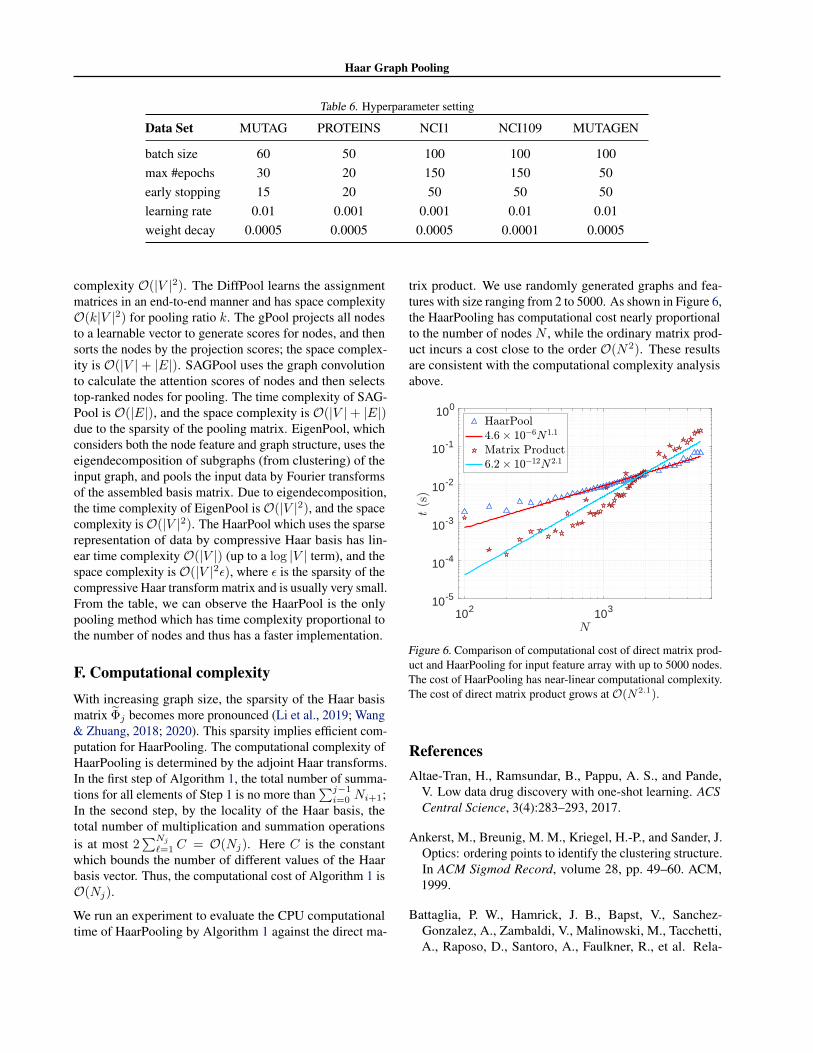
We run an experiment to evaluate the CPU computationaltime of HaarPooling by Algorithm 1 against the direct ma-

trix product. We use randomly generated graphs and fea-tures with size ranging from 2 to 5000. As shown in Figure 6,the HaarPooling has computational cost nearly proportionalto the number of nodes N , while the ordinary matrix prod-uct incurs a cost close to the order O(N2). These resultsare consistent with the computational complexity analysisabove.

102 10310-5

10-4

10-3

10-2

10-1

100

Figure 6. Comparison of computational cost of direct matrix prod-uct and HaarPooling for input feature array with up to 5000 nodes.The cost of HaarPooling has near-linear computational complexity.The cost of direct matrix product grows at O(N2.1).

ReferencesAltae-Tran, H., Ramsundar, B., Pappu, A. S., and Pande,

V. Low data drug discovery with one-shot learning. ACSCentral Science, 3(4):283–293, 2017.

Ankerst, M., Breunig, M. M., Kriegel, H.-P., and Sander, J.Optics: ordering points to identify the clustering structure.In ACM Sigmod Record, volume 28, pp. 49–60. ACM,1999.

Battaglia, P. W., Hamrick, J. B., Bapst, V., Sanchez-Gonzalez, A., Zambaldi, V., Malinowski, M., Tacchetti,A., Raposo, D., Santoro, A., Faulkner, R., et al. Rela-

Haar Graph Pooling

Table 7. Property comparison for pooling methods

Method Time Complexity Space Com-plexity

Clustering-based Spectral-based

HierarchicalPooling

Use NodeFeature

Use GraphStructure

Sparse Rep-resentation

SortPool O(|V |2) O(|V |) XDiffPool O(|V |2) O(k|V |2) X XgPool O(|V |2) O(|V | + |E|) X XSAGPool O(|E|) O(|V | + |E|) X X XEigenPool O(|V |2) O(|V |2) X X X X X

HaarPool O(|V |) O(|V |2ε) X X X X X X

‘|V |’ is the number of vertices of the input graph; ‘|E|’ is the number of edges of the input graph; ‘ε’ in HaarPooling is the sparsity ofthe compressive Haar transform matrix; ‘k’ in the DiffPool is the pooling ratio.

tional inductive biases, deep learning, and graph networks.arXiv preprint arXiv:1806.01261, 2018.

Belkin, M., Niyogi, P., and Sindhwani, V. Manifold regular-ization: A geometric framework for learning from labeledand unlabeled examples. Journal of Machine LearningResearch, 7(Nov):2399–2434, 2006.

Blum, L. C. and Reymond, J.-L. 970 million druglike smallmolecules for virtual screening in the chemical universedatabase GDB-13. Journal of the American ChemicalSociety, 131:8732, 2009.

Borgwardt, K. M., Ong, C. S., Schonauer, S., Vishwanathan,S., Smola, A. J., and Kriegel, H.-P. Protein functionprediction via graph kernels. Bioinformatics, 21(suppl 1):i47–i56, 2005.

Breiman, L. Random forests. Machine Learning, 45(1):5–32, 2001.

Bronstein, M. M., Bruna, J., LeCun, Y., Szlam, A., and Van-dergheynst, P. Geometric deep learning: going beyondeuclidean data. IEEE Signal Processing Magazine, 34(4):18–42, 2017.

Cangea, C., Velickovic, P., Jovanovic, N., Kipf, T., and Lio,P. Towards sparse hierarchical graph classifiers. In Work-shop on Relational Representation Learning, NeurIPS,2018.

Chui, C., Filbir, F., and Mhaskar, H. Representation offunctions on big data: graphs and trees. Applied andComputational Harmonic Analysis, 38(3):489–509, 2015.

Chui, C. K., Mhaskar, H., and Zhuang, X. Representationof functions on big data associated with directed graphs.Applied and Computational Harmonic Analysis, 44(1):165–188, 2018. ISSN 1063-5203. doi: https://doi.org/10.1016/j.acha.2016.12.005.

Chung, F. R. and Graham, F. C. Spectral graph theory.American Mathematical Society, 1997.

Cortes, C. and Vapnik, V. Support-vector networks. Ma-chine Learning, 20(3):273–297, 1995.

Daubechies, I. Ten lectures on wavelets. SIAM, 1992.

Debnath, A. K., Lopez de Compadre, R. L., Debnath, G.,Shusterman, A. J., and Hansch, C. Structure-activity rela-tionship of mutagenic aromatic and heteroaromatic nitrocompounds. correlation with molecular orbital energiesand hydrophobicity. Journal of Medicinal Chemistry, 34(2):786–797, 1991. doi: 10.1021/jm00106a046.

Defferrard, M., Bresson, X., and Vandergheynst, P. Con-volutional neural networks on graphs with fast localizedspectral filtering. In NIPS, pp. 3844–3852, 2016.

Diehl, F., Brunner, T., Le, M. T., and Knoll, A. Towardsgraph pooling by edge contraction. In ICML 2019 Work-shop on Learning and Reasoning with Graph-StructuredRepresentation, 2019.

Dobson, P. D. and Doig, A. J. Distinguishing enzyme struc-tures from non-enzymes without alignments. Journal ofMolecular Biology, 330(4):771–783, 2003.

Duvenaud, D. K., Maclaurin, D., Iparraguirre, J., Bom-barell, R., Hirzel, T., Aspuru-Guzik, A., and Adams, R. P.Convolutional networks on graphs for learning molecularfingerprints. In NIPS, pp. 2224–2232, 2015.

Ester, M., Kriegel, H.-P., Sander, J., Xu, X., et al. A density-based algorithm for discovering clusters in large spatialdatabases with noise. In KDD, volume 96, pp. 226–231,1996.

Fey, M. and Lenssen, J. E. Fast graph representation learningwith pytorch geometric. In Workshop on RepresentationLearning on Graphs and Manifolds, ICLR, 2019.

Gao, H. and Ji, S. Graph U-Nets. ICML, pp. 2083–2092,2019.

Haar Graph Pooling

Gilmer, J., Schoenholz, S. S., Riley, P. F., Vinyals, O., andDahl, G. E. Neural message passing for quantum chem-istry. In ICML, pp. 1263–1272, 2017.

Haar, A. Zur theorie der orthogonalen funktionensysteme.Mathematische Annalen, 69(3):331–371, 1910.

Hammond, D. K., Vandergheynst, P., and Gribonval, R.Wavelets on graphs via spectral graph theory. Appliedand Computational Harmonic Analysis, 30(2):129–150,2011.

Karypis, G. and Kumar, V. A fast and high quality multilevelscheme for partitioning irregular graphs. SIAM Journalon Scientific Computing, 20(1):359–392, 1998.

Kazius, J., McGuire, R., and Bursi, R. Derivation andvalidation of toxicophores for mutagenicity prediction.Journal of Medicinal Chemistry, 48(1):312–320, 2005.

Kersting, K., Kriege, N. M., Morris, C., Mutzel, P.,and Neumann, M. Benchmark data sets for graphkernels, 2016. URL http://graphkernels.cs.tu-dortmund.de.

Kingma, D. P. and Ba, J. Adam: A method for stochasticoptimization. In ICLR, 2015.

Kipf, T. N. and Welling, M. Semi-supervised classificationwith graph convolutional networks. In ICLR, 2017.

Knyazev, B., Taylor, G. W., and Amer, M. R. Understandingattention and generalization in graph neural networks. InNeurIPS, 2019.

Kriege, N. and Mutzel, P. Subgraph matching kernels forattributed graphs. In ICML, pp. 291–298, 2012.

Lee, J., Lee, I., and Kang, J. Self-attention graph pooling.In ICML, pp. 3734–3743, 2019.

Li, M., Ma, Z., Wang, Y. G., and Zhuang, X. Fast Haartransforms for graph neural networks. arXiv preprintarXiv:1907.04786, 2019.

Ma, Y., Wang, S., Aggarwal, C. C., and Tang, J. Graphconvolutional networks with EigenPooling. In KDD, pp.723–731, 2019a.

Ma, Z., Li, M., and Wang, Y. G. PAN: Path integral basedconvolution for deep graph neural networks. In ICML2019 Workshop on Learning and Reasoning with Graph-Structured Representation, 2019b.

Noutahi, E., Beani, D., Horwood, J., and Tossou, P. Towardsinterpretable sparse graph representation learning withLaplacian pooling. arXiv preprint arXiv:1905.11577,2019.

Pakhira, M. K. A linear time-complexity k-means algorithmusing cluster shifting. In 2014 International Conferenceon Computational Intelligence and Communication Net-works, pp. 1047–1051, 2014. doi: 10.1109/CICN.2014.220.

Ramsundar, B., Kearnes, S., Riley, P., Webster, D., Konerd-ing, D., and Pande, V. Massively multitask networks fordrug discovery. arXiv preprint arXiv:1502.02072, 2015.

Riesen, K. and Bunke, H. IAM graph database repositoryfor graph based pattern recognition and machine learn-ing. In Joint IAPR International Workshops on StatisticalTechniques in Pattern Recognition (SPR) and Structuraland Syntactic Pattern Recognition (SSPR), pp. 287–297.Springer, 2008.

Rupp, M., Tkatchenko, A., Muller, K.-R., and von Lilien-feld, O. A. Fast and accurate modeling of molecularatomization energies with machine learning. PhysicalReview Letters, 108:058301, 2012.

Shchur, O., Mumme, M., Bojchevski, A., and Gunnemann,S. Pitfalls of graph neural network evaluation. In Work-shop on Relational Representation Learning, NeurIPS,2018.

Shi, J. and Malik, J. Normalized cuts and image segmenta-tion. Departmental Papers (CIS), pp. 107, 2000.

Vinyals, O., Bengio, S., and Kudlur, M. Order matters:Sequence to sequence for sets. In ICLR, 2015.

Wale, N., Watson, I. A., and Karypis, G. Comparison ofdescriptor spaces for chemical compound retrieval andclassification. Knowledge and Information Systems, 14(3):347–375, 2008.

Wang, Y. G. and Zhuang, X. Multiresolution data analy-sis on graphs: decimated framelets and fast G-framelettransforms. arXiv, 2018.

Wang, Y. G. and Zhuang, X. Tight framelets on graphs formultiscale analysis. In Wavelets and Sparsity XVIII, SPIEProc., pp. 11138–11, 2019.

Wang, Y. G. and Zhuang, X. Tight framelets and fastframelet filter bank transforms on manifolds. Applied andComputational Harmonic Analysis, 48(1):64–95, 2020.

Wu, Z., Ramsundar, B., Feinberg, E. N., Gomes, J., Ge-niesse, C., Pappu, A. S., Leswing, K., and Pande, V.MoleculeNet: a benchmark for molecular machine learn-ing. Chemical Science, 9(2):513–530, 2018.

Wu, Z., Pan, S., Chen, F., Long, G., Zhang, C., and Yu, P. S.A comprehensive survey on graph neural networks. arXivpreprint arXiv:1901.00596, 2019.

Haar Graph Pooling

Xu, K., Hu, W., Leskovec, J., and Jegelka, S. How powerfulare graph neural networks? In ICLR, 2019.

Ying, Z., You, J., Morris, C., Ren, X., Hamilton, W., andLeskovec, J. Hierarchical graph representation learningwith differentiable pooling. In NeurIPS, pp. 4800–4810,2018.

Yuan, H. and Ji, S. Structpool: Structured graph pooling viaconditional random fields. In ICLR, 2020.

Zhang, M., Cui, Z., Neumann, M., and Chen, Y. An end-to-end deep learning architecture for graph classification. InThirty-Second AAAI Conference on Artificial Intelligence,2018a.

Zhang, Z., Cui, P., and Zhu, W. Deep learning on graphs: Asurvey. arXiv preprint arXiv:1812.04202, 2018b.

Zhou, J., Cui, G., Zhang, Z., Yang, C., Liu, Z., and Sun,M. Graph neural networks: A review of methods andapplications. arXiv preprint arXiv:1812.08434, 2018.