habitat assessment report for candidate phase 1 areas … · this habitat assessment report for...
TRANSCRIPT
R E P O R T
Habitat Assessment Report for Candidate Phase 1 Areas
Hudson River PCBs Superfund Site
General Electric CompanyAlbany, New York
November 2005
BLASLAND, BOUCK & LEE, INC. EXPONENT, INC. engineers, scientists, economists 1
Table of Contents
Acronyms ....................................................................................................................................... 1
Section 1. Introduction ............................................................................................................... 1-1
1.1 Site Background .............................................................................................................. 1-1 1.2 Goal of Habitat Assessment ............................................................................................ 1-1 1.3 Data Quality Objectives and Scope of this Report .......................................................... 1-2 1.4 Report Objectives ............................................................................................................ 1-4 1.5 Format of Phase 1 HA Report ......................................................................................... 1-5
Section 2. Habitat Assessment Approach ................................................................................ 2-1
2.1 Sampling Design and Station Selection .......................................................................... 2-1 2.2 Assessment Methodology ............................................................................................... 2-3
2.2.1 Unconsolidated River Bottom............................................................................. 2-3 2.2.2 Aquatic Vegetation Beds .................................................................................... 2-4 2.2.3 Shorelines........................................................................................................... 2-5 2.2.4 Riverine Fringing Wetlands ................................................................................ 2-5 2.2.5 Fish and Wildlife Observations........................................................................... 2-6
Section 3. Habitat Assessment Results .................................................................................... 3-1
3.1 Unconsolidated River Bottom.......................................................................................... 3-1 3.2 Aquatic Vegetation Beds ................................................................................................. 3-3 3.3 Shorelines........................................................................................................................ 3-9 3.4 Riverine Fringing Wetlands ........................................................................................... 3-12 3.5 Fish and Wildlife Observations ...................................................................................... 3-14
Section 4. FCI Models ................................................................................................................. 4-1
4.1 Unconsolidated River Bottom.......................................................................................... 4-3 4.1.1 Introduction......................................................................................................... 4-3 4.1.2 FCI Models Based on Candidate Phase 1 Area Data........................................ 4-4
4.2 Aquatic Vegetation Beds ................................................................................................. 4-6 4.2.1 Introduction......................................................................................................... 4-6 4.2.2 FCI Models Based on Candidate Phase 1 Area Data........................................ 4-7
4.3 Shorelines...................................................................................................................... 4-10 4.3.1 Introduction....................................................................................................... 4-10 4.3.2 FCI Models Based on Candidate Phase 1 Area Data...................................... 4-10
4.4 Riverine Fringing Wetlands ........................................................................................... 4-12 4.4.1 Introduction....................................................................................................... 4-12 4.4.2 FCI Models Based on Candidate Phase 1 Area Data...................................... 4-13
4.5 Current Status and Future Use of FCI Models .............................................................. 4-17 4.6 Success Criteria for Habitat Replacement and Reconstruction .................................... 4-19
Section 5. Supporting Data for HSI Models .............................................................................. 5-1

BLASLAND, BOUCK & LEE, INC. EXPONENT, INC. engineers, scientists, economists 2
Section 6. Data Needs for Phase 1 Areas.................................................................................. 6-1
6.1 Spot-Checking and Reassessment in 2004 .................................................................... 6-1 6.2 Assessments in Remaining Phase 1 Areas .................................................................... 6-2 6.3 Data Needs for FCI Models ............................................................................................. 6-3
6.3.1 Current Velocity .................................................................................................. 6-4 6.3.2 Inundation Period ............................................................................................... 6-4 6.3.3 Validation of FCI Models .................................................................................... 6-5
6.4 Data Needs for HSI Models............................................................................................. 6-6 6.5 Assessments in Off-Site Reference Areas ...................................................................... 6-7 6.6 Spot-Checking and Reassessment in Subsequent Seasons.......................................... 6-7 6.7 Schedule.......................................................................................................................... 6-8
Section 7. References ................................................................................................................. 7-1
Tables (placed in text) 1 Unconsolidated River Bottom Stations for Detailed Functional Assessments 2 Range of Conditions Observed in Unconsolidated River Bottoms in the Upper Hudson River 3 Aquatic Vegetation Bed Stations for Detailed Functional Assessments 4 Percent Cover of Aquatic Vegetation in the Thompson Island Pool (River Reach 1; Law Environmental
1991) 5 Significance Levels for Spearman Rank Correlation of Aquatic Vegetation Bed Parameters 6 Range of Conditions in Aquatic Vegetation Beds in the Upper Hudson River 7 Shoreline Stations for Detailed Functional Assessments 8 Range of Conditions Observed in Shorelines in the Upper Hudson River 9 Riverine Fringing Wetland Stations for Detailed Functional Assessments 10 Range of Conditions Observed in Riverine Fringing Wetlands in the Upper Hudson River 11 Fish and Wildlife Species Observed During Habitat Assessments 12 Unconsolidated River Bottom Measured Variables and FCI Models 13 Aquatic Vegetation Bed Habitat Measured Variables and FCI Models 14 Shoreline Habitat Measured Variables and FCI Models 15 Wetland Habitat Measured Variables and FCI Models 16 Calculated FCI Values for Phase 1 Areas 17 List of Species for HSI Models 18 Calculated FCI Values for Areas Assessed in 2003 and Reassessed in 2004 Figures 1 Upper Hudson River 2 Sampling Station Locations for Habitat Assessments in the Phase 1 Areas 3 Sampling Station Locations for Habitat Assessments in the Phase 1 Areas 4 Sampling Station Locations for Habitat Assessments in the Phase 1 Areas 5 Total Organic Carbon (TOC) and Percent Fines at Phase 1 Areas and Assessment Stations Appendices A Standard Operating Procedure for Unconsolidated (Non-Vegetated) River Bottom Assessment B Standard Operating Procedure for Aquatic Bed Assessment C Standard Operating Procedure for Natural Shoreline Assessment D Standard Operating Procedure for Fringing Wetland Assessment E Fish and Wildlife Survey Form F Geographic Coordinates and Species for Assessment Stations G Tables for Habitat Assessment Data H Transformation of Field Data to Subindices
BLASLAND, BOUCK & LEE, INC. EXPONENT, INC. engineers, scientists, economists 3
I Habitat Suitability Index Models for Key Species J Wetland Coring Logs K Tables for Habitat Reassessment Data from 2004 L Completed Fish and Wildlife Observation Forms M Statistical Analysis - Submerged Aquatic Vegetation

BLASLAND, BOUCK & LEE, INC. EXPONENT, INC. engineers, scientists, economists 1
Acronyms BBL = Blasland, Bouck & Lee, Inc.
BMI = benthic macroinvertebrate
BMP = Baseline Monitoring Program
cfs = cubic feet per second
cm = centimeter
cm2 = square centimeter
DO = dissolved oxygen
DQO = data quality objective
ESUH = Especially Sensitive or Unique Habitat
fps = feet per second
FCI = Functional Capacity Index
GE = General Electric Company
g/cm3 = grams per cubic centimeter
g/m2 = grams per square meter
GI = Griffin Island
GIA = Griffin Island Area
HD Report = Habitat Delineation Report
HDA Work Plan = Habitat Delineation and Assessment Work Plan
HSI = Habitat Suitability Index
HGM = hydrogeomorphic
Kd = light extinction coefficient
LWD = Large woody debris
m = meter
m2 = square meter
mg/kg = milligrams per kilogram
mg/L = milligrams per liter
ND = Northumberland Dam
NDA = Northumberland Dam Area
NOAA = National Oceanic and Atmospheric Administration
NTIP = Northern Thompson Island Pool
NWI = National Wetland Inventory

BLASLAND, BOUCK & LEE, INC. EXPONENT, INC. engineers, scientists, economists 2
NYSDEC = New York State Department of Environmental Conservation
Phase 1 DAD Report = Phase 1 Dredge Area Delineation Report
Phase 2 DAD Report = Phase 2 Dredge Area Delineation Report
Phase 1 HA Report = Habitat Assessment Report for Candidate Phase 1 Areas
Phase 2 HA Report = Habitat Assessment Report for Phase 2 Areas
PMI = phytophilous macroinvertebrate
QEA = Quantitative Environmental Analysis, LLC
RD = remedial design
RD AOC = Remedial Design Administrative Order of Consent
RD Work Plan = Remedial Design Work Plan
RM = River Mile
ROD = Record of Decision
RS = River Section
RTE = rare, threatened, or endangered
SAV = submerged aquatic vegetation
SEDC = Supplemental Engineering Data Collection
shoots/m2 = shoots per square meter
SOPs = Standard Operating Procedures
SSAP = Sediment Sampling and Analysis Program
SSS = side-scan sonar
TOC = total organic carbon
USEPA = United States Environmental Protection Agency
USFWS = U.S. Fish and Wildlife Service
BLASLAND, BOUCK & LEE, INC. EXPONENT, INC. engineers, scientists, economists 1-1
1. Introduction
1.1 Site Background This Habitat Assessment Report for Candidate Phase 1 Areas (Phase 1 HA Report) is submitted by the General
Electric Company (GE) as part of the remedial design (RD) program for the remedy selected by the United
States Environmental Protection Agency (USEPA) for the Upper Hudson River. The RD program is established
in the Remedial Design Work Plan (RD Work Plan) (Blasland, Bouck & Lee, Inc. [BBL], 2003a). Unless stated
otherwise, the approach to the habitat assessments described in this Phase 1 HA Report follows the scope of
work described in the Habitat Delineation and Assessment Work Plan (HDA Work Plan) (BBL, 2003b) and
Attachments A through D thereto (reprinted for convenience as Appendices A through D of this Phase 1 HA
Report). Both the RD Work Plan and the HDA Work Plan are part of the Administrative Order on Consent for
Remedial Design (RD AOC) (USEPA/GE, 2003), which was executed in August 2003.
On February 1, 2002, the USEPA issued a Superfund Record of Decision (ROD) that calls for, among other
things, the removal of substantial quantities of PCB-containing sediments from the Upper Hudson River
(USEPA, 2002). In the ROD, the USEPA divided the Upper Hudson River into three sections (River Section 1,
River Section 2, and River Section 3) (hereinafter referred to as the “Upper Hudson River” or the “project
area”). These sections, illustrated on Figure 1, are defined as follows:
• River Section 1: Former location of Fort Edward Dam to Thompson Island Dam (approximately 6.3 miles);
• River Section 2: Thompson Island Dam to Northumberland Dam (ND) (approximately 5.1 miles); and
• River Section 3: ND to the Federal Dam at Troy (approximately 29.5 miles).
1.2 Goal of Habitat Assessment The goal of the habitat assessment, as described in the HDA Work Plan, is to collect information on habitat
specific physical and biological variables, listed in Table 2 of that Work Plan, that are related to the ecological
functions provided by those habitats in reference areas and areas that are potentially affected by sediment
removal activities. This information will be used to develop the basis of design for habitat replacement and
reconstruction in Phase 1 areas and to determine when post-remediation habitat conditions fall within the ranges
of reference conditions.

BLASLAND, BOUCK & LEE, INC. EXPONENT, INC. engineers, scientists, economists 1-2
To quantify the ecological functions within the Upper Hudson River habitats, the assessment procedures focused
on direct measurements of the specified physical and biological parameters in the habitats. These parameters
include both structural and functional attributes of the habitats. The concept that these types of parameters can
be used to quantify ecological functions is one of the foundations of the hydrogeomorphic (HGM) approach
(Shafer and Yozzo, 1998; Ainslie et al., 1999; Smith and Wakeley, 2001; Clairain, 2002) and habitat evaluation
procedures (e.g., Habitat Suitability Indices [HSIs]), and is used in aquatic habitat monitoring and restoration
programs (Niedowski, 2000; Fonseca et al., 2000). As recommended by those programs, the parameters listed
in Table 2 of the HDA Work Plan include measures of both structural and functional parameters (as discussed
further in Section 4 below).
1.3 Data Quality Objectives and Scope of this Report The data quality objectives (DQOs) for the habitat assessment program, as set forth in the HDA Work Plan, are
to:
• Determine the range of structural parameters that are relevant to and associated with ecological functions
within each habitat type;
• Define the relationships between selected structural parameters and ecological functions within each habitat
type; and
• Develop a database of habitat-specific data to facilitate subsequent identification and establishment of
design criteria, success criteria, and monitoring requirements for the habitat replacement and reconstruction
program.
These DQOs require that data on the specified parameters of habitats be collected following the assessment
protocols included in Appendices A through D of this Phase 1 HA Report. Data included in this report were
collected from September 8 to October 1, 2003 and September 14 to September 20, 2004. The remainder of the
Phase 1 data was collected in September 2005. The 2005 data will be reported in the Phase 1 Final Design
Report. Data collection from Phase 2 areas was initiated in September 2005 and will be completed in
subsequent years to fulfill the HDA Program as described in the HDA Work Plan. Phase 2 habitat assessment
data will be reported in a Habitat Assessment Report for Phase 2 Areas (Phase 2 HA Report).
As described in the HDA Work Plan, habitats were assessed as:

BLASLAND, BOUCK & LEE, INC. EXPONENT, INC. engineers, scientists, economists 1-3
• Unconsolidated (unvegetated) river bottom;
• Aquatic vegetation beds;
• Shoreline habitats, including maintained and natural shorelines; and
• Wetland habitats, specifically riverine fringing wetlands.
The HDA Work Plan required that, in the field season immediately following the execution of the RD AOC
(2003), GE conduct habitat delineation activities for all three river sections and also conduct habitat assessment
activities for the “candidate Phase 1 areas,” which were identified in the RA Work Plan as: 1) the upper portion
of the Thompson Island Pool (Northern TIP or NTIP) in River Section 1; 2) the Griffin Island Area (GIA) in
River Section 1; and 3) and the areas of River Section 2 in the vicinity of Hot Spots 33-35, known as the
Northumberland Dam Area (NDA). In 2003, GE conducted the habitat delineation activities throughout the
project area and, due to time and seasonal constraints, conducted habitat assessment activities at a subset of the
candidate Phase 1 areas and certain available reference habitats. At the time that prior versions of this Phase 1
HA Report were submitted to USEPA in April and September 2004, all three candidate Phase 1 areas were still
under consideration. Subsequently, GE submitted a revised Phase 1 Target Area Identification Report (Phase 1
TAI Report) (Quantitative Environmental Analysis, LLC [QEA], 2004), which proposed that Phase 1 consist of:
1) the most upstream dredge areas in the NTIP; and 2) the portion of the GIA on the east side of Griffin Island
(GI). USEPA approved that proposal in a letter of January 20, 2005. Nevertheless, since the habitat assessment
activities conducted to date included stations in all three of the candidate Phase 1 areas, this Phase 1 HA Report
continues to include the data and results from the assessment activities conducted in those candidate Phase 1
areas. Simultaneously with the submission of this Phase 1 HA Report, GE is submitting as a separate document,
the Habitat Delineation Report (BBL and Exponent, 2005a) (HD Report), which provides the results of the
habitat delineation activities conducted in all river sections, as well as an evaluation of off-site reference areas
outside the project area.
In August 2005, GE submitted a Supplemental Habitat Assessment Work Plan (SHAWP) to USEPA and
finalized that SHAWP in September 2005 (BBL and Exponent, 2005b). The SHAWP presented GE’s proposed
approach and locations for conducting detailed habitat assessment activities in the Phase 1 areas (as defined in
the approved Phase 1 TAI Report) and in the Phase 2 dredging areas, as well as in suitable reference areas. The
SHAWP noted that the proposed Phase 2 assessment station locations and associated reference locations are
subject to change following completion and USEPA approval of the Phase 2 Dredge Area Delineation Report
(Phase 2 DAD Report). The SHAWP was approved by USEPA on November 17, 2005. The additional
assessment activities in Phase 1 areas were completed in September 2005. Assessment activities at Phase 2

BLASLAND, BOUCK & LEE, INC. EXPONENT, INC. engineers, scientists, economists 1-4
areas were initiated in September 2005. Assessment activities at remaining Phase 2 areas, associated reference
areas, and off-site reference areas will be completed following completion and USEPA approval of the Phase 2
Dredge Area Delineation Report (Phase 2 DAD Report). As indicated above, the results of subsequent
assessments as they pertain to the remaining Phase 1 areas will be presented in the Phase 1 Final Design Report,
and the results of the assessments for Phase 2 areas will be presented in a Phase 2 HA Report.
Habitat delineation and assessment tasks for the land-based sediment and water processing facilities and
associated terrestrial access routes to the river are beyond the scope of this Phase 1 HA Report; these tasks were
conducted by the USEPA (Ecology and Environment, 2003).
1.4 Report Objectives The objectives of this Phase 1 HA Report are to:
• Document the habitat assessment results for candidate Phase 1 areas that were assessed in 2003 and 2004, in
accordance with the procedures detailed in the HDA Work Plan;
• Present the Functional Capacity Index (FCI) models based on data collected in 2003 and those based on data
collected in 2004 from the Phase 1 areas; and
• Present HSI models from the U.S. Fish and Wildlife Service (USFWS) that will be used to supplement FCI
models for the wildlife habitat (habitat suitability) function for representative species.
This Phase 1 HA Report provides the foundation for implementing the habitat replacement and reconstruction
program for the Phase 1 areas. As stated in the HDA Work Plan, the overall goal of that program is “to replace
the functions of the Upper Hudson River habitats that are affected by dredging to within the range of functions
found in similar physical settings in the Upper Hudson River, given the changes in river conditions that will
result from remedy implementation or from other factors” (BBL, 2003b). The habitat-specific variables
summarized in Section 3 of this Phase 1 HA Report provide the underlying data that will be used for developing
the basis of design for habitat replacement and reconstruction in the candidate Phase 1 areas. Details of
additional factors important to the habitat replacement and reconstruction will be provided in the Adaptive
Management Plans, which will be part of the Phase 1 and Phase 2 Final Design Reports.
The associated FCI models and HSI models are the fundamental tools that will be used to assess whether the
overall program goals have been met once the habitat replacement and reconstruction designs have been
BLASLAND, BOUCK & LEE, INC. EXPONENT, INC. engineers, scientists, economists 1-5
implemented. In addition, secondary success criteria (e.g., based on quantitative observations of fish and
wildlife presence and abundance) may be used if the primary criteria based on the above models and the
measured parameters used in them are not indicative of success.
1.5 Format of Phase 1 HA Report The remainder of this Phase 1 HA Report consists of the following six sections:
• Section 2 describes the overall approach, sources of information, and methods used to conduct the
assessments for each habitat type;
• Section 3 describes the results of the habitat assessments conducted in 2003 and 2004 in the candidate Phase
1 areas;
• Section 4 describes the overall approach, sources of information, and methods used to develop the FCI
models for each habitat;
• Section 5 describes the HSI models that will be used;
• Section 6 describes additional data needs for the Phase 1 areas; and
• Section 7 lists the references used to prepare this Phase 1 HA Report.
In addition, several appendices are included in this report to provide more detailed information on the habitat
assessment activities and underlying data.
This Phase 1 HA Report uses English and metric units of measurement consistent with the standard practice for
the data being reported and in accordance with the methods described in the Standard Operating Procedures
(SOPs) from the HDA Work Plan. Where appropriate, English conversions are applied to metric units reported
in the text or shown in the tables.

BLASLAND, BOUCK & LEE, INC. EXPONENT, INC. engineers, scientists, economists 2-1
2. Habitat Assessment Approach
2.1 Sampling Design and Station Selection The four habitat types (i.e., unconsolidated river bottom, aquatic vegetation beds, shoreline, and fringing
wetlands) of the Upper Hudson River potentially impacted by the sediment removal activities were assessed in
accordance with procedures outlined in the HDA Work Plan. Ultimately, habitat assessments will be completed
in representative areas for each habitat type in both Phase 1 and Phase 2 areas, prior to the commencement of
the dredging in each area, respectively. The HDA Work Plan stated that assessments were to be completed at
136 unconsolidated river bottom, 52 aquatic vegetation bed, 68 shoreline, and 10 fringing wetland habitat
stations. Based on subsequent field work, the number of riverine fringing wetland stations was increased to 16
to include some areas identified as especially sensitive or unique habitats (ESUH) and to represent a greater
variety of wetlands. In addition, riverine fringing wetland stations greater than 0.5 acre (only present in Phase 2
areas) and aquatic vegetation beds greater than 3 acres were/will be sampled at two locations within each station
to evaluate variability within wetlands/aquatic vegetation beds (BBL and Exponent, 2005b). Therefore, the
number of unconsolidated river bottom stations was reduced to 100 stations to compensate for the greater
number of riverine fringing wetland and aquatic vegetation bed stations. Nine samples are to be collected from
within each unconsolidated river bottom, aquatic vegetation bed, and riverine fringing wetland station; three
transects are to be used at each shoreline station (see Appendices A through E for specifics on the sample
design).
The main text of this Phase 1 HA Report describes the results of the habitat assessments that were completed in
2003 for a subset of candidate Phase 1 areas and reference areas (i.e., areas that are not expected to be directly
affected by the sediment removal activities) at six unconsolidated river bottom, nine aquatic vegetation bed, 14
shoreline, and four fringing wetland habitat stations. The number of stations assessed in 2003 was limited due
to the seasonal restrictions prescribed in the HDA Work Plan and signing of the Administrative Order on
Consent for Hudson River Remedial Design and Cost Recovery (RD AOC) on August 13, 2003. Field work
was initiated immediately following the signing of the RD AOC. The first effort involved groundtruthing the
aerial photographs (which were taken “at risk” by GE prior to the signing of the RD AOC). Identification of
target and reference stations for subsequent assessment sampling was not possible until that work was
completed. Once the target and reference stations were identified, fieldwork was scheduled to maximize the
number of stations that could be sampled within each habitat before the seasonal window closed. In addition,
collection of data from target stations was prioritized over collection of data from reference stations. However,

BLASLAND, BOUCK & LEE, INC. EXPONENT, INC. engineers, scientists, economists 2-2
at the time of the 2003 sampling, all stations effectively represent “reference” conditions because no dredging
had occurred.
In addition to the habitat assessment work conducted in 2003, several stations that were assessed in that year
were spot-checked and reassessed in 2004. That reassessment effort is described further in subsection 6.1. The
data from that reassessment are presented in Appendix K and area also included, in summary form, in the tables
in Section 3 of this report.
Detailed habitat assessment activities were completed in September 2005 in the remaining Phase 1 areas (as
defined in the approved Phase 1 TAI Report) that were not sampled in 2003 and 2004. Due to time constraints,
the results of those assessments are not included in this Phase 1 HA Report, but will be included in the Phase 1
Final Design Report. Habitat assessment activities in additional suitable reference areas, off-site reference
areas, and data gap areas (if necessary) will be conducted in 2006. The results of those additional assessment
activities will be incorporated into the Phase 2 HA Report.
As described in the HDA Work Plan and its Attachments A through D (Appendices A through D of this Phase 1
HA Report), sampling stations for each habitat type were selected to meet the following criteria:
• Adequately characterize habitat strata identified from the habitat delineation information;
• Include an equal number of target stations (in proposed dredge areas) and reference stations (outside of
proposed dredge areas); and
• Be allocated among river sections in rough proportion to the relative areas of the habitat to be dredged (i.e.,
potentially affected habitat) in each river section.
To select specific target and reference stations for each habitat type, information from the field verification
activities conducted to delineate the habitats in the project area, existing habitat information (e.g., New York
State Department of Environmental Conservation [NYSDEC] wetland maps), and data from the Sediment
Sampling and Analysis Program (SSAP) were integrated into a series of overlay maps. These maps were then
compared with the proposed dredge area delineations that were in production as working drafts for the Phase 1
DAD Report to identify sampling locations for the detailed habitat assessment activities. Specific habitat station
locations were selected based on sediment type, overlying water depth, adjacent land use, and proximity to other
habitat features (e.g., NYSDEC wetlands). In addition, stations were selected to include both target stations
(i.e., in proposed dredge locations) and reference stations (i.e., outside of proposed dredge locations). All

BLASLAND, BOUCK & LEE, INC. EXPONENT, INC. engineers, scientists, economists 2-3
reference stations described in this Phase 1 HA Report are on-site reference stations. Target or reference
stations are selected in equal numbers by river section and not by Phase 1 and Phase 2 areas; however, until
remediation begins, all samples are collected under “reference” conditions (i.e., unimpacted by remedial
activities). If changes are made to dredge areas prior to the start of remediation activities, the stations may be
reallocated; therefore, the designation of these stations as target and reference is subject to change. Off-site
reference stations were investigated in 2003 (see subsection 3.2 of the HD Report [BBL and Exponent, 2004]
and subsection 6.5 of this report for more information), and will be sampled in the 2006 field season.
The specific locations selected for detailed assessment activities for the unconsolidated river bottom, aquatic
vegetation bed, shoreline, and riverine fringing wetland habitat types were randomly selected from the stations
identified in the candidate Phase 1 areas as described above, in accordance with the respective SOPs. The
specific locations of the assessment stations are shown on the maps provided as Figures 2 through 4 and
described in more detail in Section 3 below. Figures 2 through 4 consist of maps of the three candidate Phase 1
areas and show the habitat delineation features described in the HD Report (BBL and Exponent, 2004). The
specific assessment locations for each habitat type have been added to these maps.
2.2 Assessment Methodology The following subsections describe the methods used to assess:
• Unconsolidated river bottom;
• Aquatic vegetation beds;
• Shorelines;
• Riverine fringing wetlands; and
• Fish and wildlife observations.
2.2.1 Unconsolidated River Bottom Methods used to assess the unconsolidated river bottom habitats in the candidate Phase 1 areas followed the
SOP in Attachment A of the HDA Work Plan (Appendix A of this Phase 1 HA Report). Clarifications or
modifications to habitat assessment methods presented in the SOP are described below along with supporting
rationale.

BLASLAND, BOUCK & LEE, INC. EXPONENT, INC. engineers, scientists, economists 2-4
Embeddedness is the extent to which rocks (gravel, cobble, and boulders) and snags are covered or sunken into
the silt, sand, or mud of a “high gradient” stream bottom (Barbour et al., 1999). This parameter (Appendix A;
Step 5) was not evaluated in the assessment of unconsolidated river bottom habitats for candidate Phase 1 areas
due to the lack of high gradient areas.
Surface-water quality data (temperature, conductivity, dissolved oxygen [DO], pH, and turbidity) were added to
the sampling program and were recorded using a Horiba U-23 multiparameter probe. The probe was calibrated
daily and surface-water quality data were collected at each unconsolidated river bottom sampling station in
accordance with the manufacturer’s instructions included with the equipment.
Light availability and current velocity data were collected at the approximate center of each sampling station
concurrently with the assessment of the unconsolidated river bottom habitats using the same procedures
described for the aquatic vegetation bed in Appendix B. Light availability data were collected using an LI-1400
datalogger connected to an LI-190SA Quantum sensor (to record underwater light) and an LI-192SA Quantum
sensor (to record surface light levels). Current velocity was recorded using a Marsh McBirney 201
Electromagnetic flow meter.
2.2.2 Aquatic Vegetation Beds Methods used to assess the aquatic vegetation beds in the candidate Phase 1 areas followed the SOP in
Attachment B of the HDA Work Plan (Appendix B of this Phase 1 HA Report). Specific sampling locations
were randomly selected within the depth and species composition strata of the aquatic vegetation bed.
Clarifications or modifications to habitat assessment methods prescribed in the SOP are described below along
with supporting rationale.
Due to the effective date of the RD AOC, the start date for the 2003 habitat assessment work was delayed. On
August 21, 2003, GE submitted a letter to the USEPA requesting an extension of the timeframe for assessing
habitats. As indicated in the HDA Work Plan, the preferred period to conduct habitat assessments for the aquatic
vegetation bed habitat was July 15 through August 30. GE requested that the schedule be modified to allow data
collection to continue through mid-October if necessary. In a response dated August 28, 2003, the USEPA
agreed to the schedule modification. Assessments of the aquatic vegetation bed habitats in 2003 were
completed between September 22 and 29, 2003. In 2004, reassessment of a subset of those stations assessed in
2003 was conducted between September 14 through September 20. The dominant aquatic vegetation species,
BLASLAND, BOUCK & LEE, INC. EXPONENT, INC. engineers, scientists, economists 2-5
such as wild celery and pondweeds, are actively growing during this period; however, certain early-season
species of aquatic vegetation may not have been present at the time of the assessments and reassessment.
Surface-water quality data (temperature, conductivity, DO, pH, and turbidity) were added to the sampling
program and were recorded using a Horiba U-23 multiparameter probe. The probe was calibrated daily and
surface-water quality data were collected at each aquatic vegetation bed sampling station in accordance with the
manufacturer’s instructions included with the equipment.
2.2.3 Shorelines Methods used to assess the shoreline habitats in the candidate Phase 1 areas followed the SOP in Attachment C
of the HDA Work Plan (Appendix C of this Phase 1 HA Report). Transects were located within stations after
field verification of the shoreline condition as natural or maintained. Clarifications or modifications to habitat
assessment methods prescribed in the SOP are described below along with supporting rationale.
The assessment of organic shoreline substrate components in the Shoreline Substrate Assessment Protocol
(Appendix C) requires an estimate of length and width of large woody debris in contact with surface waters
within 50 meters (m) on either side of the transect. In the field, this procedure dictated the position of the three
transects at each shoreline station. Where possible, transects were placed approximately 100 m apart to avoid
transect overlap and prevent artificially inflated estimates of shoreline debris. When transects could not be
placed 100 m apart due to habitat constraints, shoreline debris measurements for each transect were taken at half
the distance to the neighboring transect.
2.2.4 Riverine Fringing Wetlands A new HGM subclass of “riverine fringing” wetlands has been used to classify the Hudson River wetlands.
Riverine fringing wetlands possess characteristics similar to traditional HGM classes of riverine and tidal fringe,
but riverine fringing wetlands have a unique combination of HGM setting and hydrodynamics. Benches or
slopes inside the river banks provide the HGM setting for riverine fringing wetlands, and within-channel flow is
the dominant water source. Hydrodynamics have both a vertical component and a horizontal component. The
vertical component results from seasonal changes in precipitation and evapotranspiration in the watershed and
episodic changes due to hydrofacilities on the river. The horizontal component results from non-tidal river flow.

BLASLAND, BOUCK & LEE, INC. EXPONENT, INC. engineers, scientists, economists 2-6
Methods used to assess the riverine fringing wetlands in the candidate Phase 1 areas followed the SOP in
Attachment D of the HDA Work Plan (Appendix D of this Phase 1 HA Report). Specific sampling locations
were randomly selected within the vegetation community strata of the fringing wetlands. Clarifications or
modifications to the fringing wetland habitat assessment methods prescribed in the HDA Work Plan are
described below along with supporting rationale.
In accordance with the HDA Work Plan, three transects were established on each assessed wetland. Transects
were used to evaluate and characterize topography and orientation of plant community zonation within each
study wetland. Sampling quadrats (i.e., a 1-square-meter [m2] sampling grid) for vegetation and soil analysis
were randomly placed within vegetation community strata identified at assessed wetlands.
The soils present in the assessed wetlands are alluvial and do not possess true O (organic) or A (topmost mineral
layer) horizons. Therefore, percent cover for O and A soil horizons was not measured as described in Appendix
D.
2.2.5 Fish and Wildlife Observations As described in the HDA Work Plan, fish and wildlife were observed at each sampling location as a distinct task
to document the occurrence of fish, birds, reptiles, amphibians, and mammals in each of the four habitat types.
Specifically, during the habitat assessment field activities, personnel experienced in identifying wildlife species
surveyed the habitat being assessed for the presence of fish or wildlife using that habitat or for signs of such
wildlife (e.g., calls, tracks, scat, slides, dens, burrows, daybeds, and huts). Field personnel observed the wildlife
from boats or on the shore depending on the type of habitat being surveyed. Field personnel began recording
their observations on approach to a station to document any wildlife flushed by the approach of the field team.
Field personnel then continued their observations for the entire duration of the sampling event, covering the
habitat-specific station and surrounding environs. Data were recorded on the Fish and Wildlife Survey Form
(Appendix E), including species name, number observed, sight code, sign code, observer’s initials, and habitat
type/location. The completed forms are provided in Appendix L.
In addition, the HDA Work Plan specifies that field personnel document the location(s) of any rare, threatened,
or endangered (RTE) species of biota or sensitive habitats observed during field activities. The ROD specifies
that the Indiana bat, Karner blue butterfly, and bald eagle have been identified by the USFWS, and the shortnose
sturgeon has been identified by the National Marine Fisheries Service (National Oceanic and Atmospheric
BLASLAND, BOUCK & LEE, INC. EXPONENT, INC. engineers, scientists, economists 2-7
Administration [NOAA] Fisheries), as those species that could be affected by the Hudson River PCB cleanup.
Queries of the Natural Heritage Program did not identify any other species of concern. At each sampling
station, the immediate and adjacent areas were observed by a dedicated wildlife biologist for the duration of the
habitat sampling (usually more than 1 hour). No investigative surveys were conducted specifically to identify
RTE species. As discussed in Section 3, the only RTE species observed was the bald eagle (Haliaeetus
leucocephalus).

BLASLAND, BOUCK & LEE, INC. EXPONENT, INC. engineers, scientists, economists 3-1
3. Habitat Assessment Results This section summarizes the results of the habitat assessment activities conducted at the selected assessment
locations within the candidate Phase 1 areas. Field data were collected from those locations between September
8 and October 1, 2003. The specific locations are listed, by geographic coordinates, in Appendix F and the data
are listed, for each habitat type, in Appendix G. Several stations were also reassessed in 2004 from September
14 through September 20. That reassessment is discussed further in subsection 6.1, and the resulting data are
summarized in the tables in this section and are presented in Appendix K. The remainder of this section
describes the 2003 assessment data in detail.
As an initial screening to determine how the sampling stations compared to other candidate Phase 1 areas, the
range of sediment total organic carbon (TOC) and percent fines data from the top 2 inches of the sediment were
compared (Figure 5). Percent fines and TOC data were obtained from the SSAP stations within 100 feet of the
nearest aquatic vegetation bed and unconsolidated river bottom sampling quadrat. Sediment samples were also
collected from within SAV beds to characterize sediment nutrient availability. This sediment interval was used
because percent fines data were available only from surficial sediment samples (0 to 2 inches) used for
groundtruthing the side-scan sonar (SSS) data. In addition, the 0-2 inch surface interval is the interval to which
recruiting macroinvertebrate and plants species are initially exposed, and the layer that is most likely to be
changed by normal river hydrodynamics. The data indicate that sediments in the unconsolidated river bottom
that were assessed have similar TOC concentrations to those generally found in the NTIP, but have somewhat
lower TOC and percent fines than those generally found in the GIA and the NDA (see Figure 5). The NTIP had
the lowest percentage of fines. Subsequent Phase 1 assessment stations will be located in areas with higher TOC
and percent fines. In addition, TOC data from deeper sediment intervals, if available from the SSAP, will be
reviewed and included in the final evaluation of Phase 1 areas in the Phase 1 Final Design Report.
3.1 Unconsolidated River Bottom Six stations were sampled between September 30 and October 1, 2003 (see Table 1, below). Five stations were
located in River Section 1 and one station was located in River Section 2 (as shown on Figures 2 through 4). At
the six stations, sand was the most common substrate often mixed with other finer types of sediment (Stations 2,
4, 5, and 6 in Table 1). Boulders were most common at sample points within Station 3 (in the river channel near
the northern tip of GI) and, within this station, were occasionally abundant (10% to 50% of total composition).
BLASLAND, BOUCK & LEE, INC. EXPONENT, INC. engineers, scientists, economists 3-2
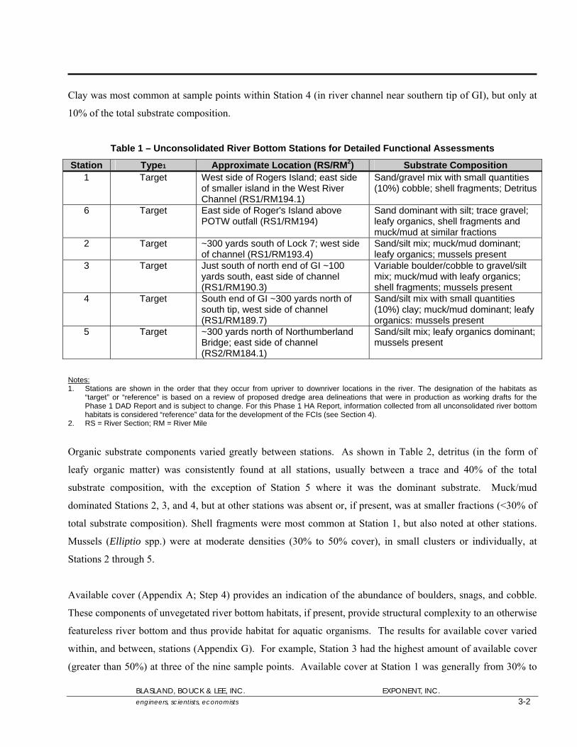
Clay was most common at sample points within Station 4 (in river channel near southern tip of GI), but only at
10% of the total substrate composition.
Table 1 – Unconsolidated River Bottom Stations for Detailed Functional Assessments
Station Type1 Approximate Location (RS/RM2) Substrate Composition 1 Target West side of Rogers Island; east side
of smaller island in the West River Channel (RS1/RM194.1)
Sand/gravel mix with small quantities (10%) cobble; shell fragments; Detritus
6 Target East side of Roger's Island above POTW outfall (RS1/RM194)
Sand dominant with silt; trace gravel; leafy organics, shell fragments and muck/mud at similar fractions
2 Target ~300 yards south of Lock 7; west side of channel (RS1/RM193.4)
Sand/silt mix; muck/mud dominant; leafy organics; mussels present
3 Target Just south of north end of GI ~100 yards south, east side of channel (RS1/RM190.3)
Variable boulder/cobble to gravel/silt mix; muck/mud with leafy organics; shell fragments; mussels present
4 Target South end of GI ~300 yards north of south tip, west side of channel (RS1/RM189.7)
Sand/silt mix with small quantities (10%) clay; muck/mud dominant; leafy organics: mussels present
5 Target ~300 yards north of Northumberland Bridge; east side of channel (RS2/RM184.1)
Sand/silt mix; leafy organics dominant; mussels present
Notes: 1. Stations are shown in the order that they occur from upriver to downriver locations in the river. The designation of the habitats as
“target” or “reference” is based on a review of proposed dredge area delineations that were in production as working drafts for the Phase 1 DAD Report and is subject to change. For this Phase 1 HA Report, information collected from all unconsolidated river bottom habitats is considered “reference” data for the development of the FCIs (see Section 4).
2. RS = River Section; RM = River Mile
Organic substrate components varied greatly between stations. As shown in Table 2, detritus (in the form of
leafy organic matter) was consistently found at all stations, usually between a trace and 40% of the total
substrate composition, with the exception of Station 5 where it was the dominant substrate. Muck/mud
dominated Stations 2, 3, and 4, but at other stations was absent or, if present, was at smaller fractions (<30% of
total substrate composition). Shell fragments were most common at Station 1, but also noted at other stations.
Mussels (Elliptio spp.) were at moderate densities (30% to 50% cover), in small clusters or individually, at
Stations 2 through 5.
Available cover (Appendix A; Step 4) provides an indication of the abundance of boulders, snags, and cobble.
These components of unvegetated river bottom habitats, if present, provide structural complexity to an otherwise
featureless river bottom and thus provide habitat for aquatic organisms. The results for available cover varied
within, and between, stations (Appendix G). For example, Station 3 had the highest amount of available cover
(greater than 50%) at three of the nine sample points. Available cover at Station 1 was generally from 30% to
BLASLAND, BOUCK & LEE, INC. EXPONENT, INC. engineers, scientists, economists 3-3
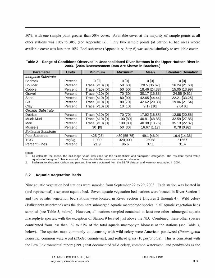
50%, with one sample point greater than 50% cover. Available cover at the majority of sample points at all
other stations was 10% to 30% (see Appendix G). Only two sample points (at Station 6) had areas where
available cover was less than 10%. Pool substrate (Appendix A; Step 6) was scored similarly to available cover.
Table 2 – Range of Conditions Observed in Unconsolidated River Bottoms in the Upper Hudson River in 2003. (2004 Reassessment Data Are Shown in Brackets.)
Parameter Units Minimum Maximum Mean Standard Deviation Inorganic Substrate Bedrock Percent 0 [0] 0 [0] 0 [0] 0 [0] Boulder Percent Trace (<10) [0] 50 [60] 20.5 [36.67] 16.24 [21.60] Cobble Percent Trace (<10) [0] 50 [50] 18.46 [24.38] 15.05 [13.99] Gravel Percent Trace (<10) [0] 70 [30] 30.17 [16.88] 24.55 [9.61] Sand Percent Trace (<10) [0] 80 [90] 42.65 [44.44] 22.21 [33.25] Silt Percent Trace (<10) [0] 80 [70] 42.62 [29.33] 19.06 [21.54] Clay Percent Trace (<10) [0] 10 [10] 9.17 [10] 2.04 [0] Organic Substrate Detritus Percent Trace (<10) [0] 70 [70] 17.92 [16.88] 12.88 [20.56] Muck-Mud Percent Trace (<10) [0] 100 [80] 40.81 [48.85] 32.59 [27.85] Marl Percent Trace (<10) [0] 100 [80] 40.38 [18.75] 35.13 [22.87] Mussels Percent 30 [0] 50 [30] 16.67 [1.17] 0.78 [0.92] Epifaunal Substrate Pool Substrate1 Percent <25 [25] >80 [55-75] 49.1 [46.9] 16.4 [14.36] TOC mg/kg 1,000 320,000 25958 51657 Percent Fines Percent 21.9 96.6 37.1 31.4
Notes: 1. To calculate the mean, the mid-range value was used for the “suboptimal” and “marginal” categories. The resultant mean value
equates to “marginal.” Trace was set to 5 to calculate the mean and standard deviation. 2. Sediment total organic carbon and percent fines were obtained from the SSAP dataset and were not resampled in 2004.
3.2 Aquatic Vegetation Beds Nine aquatic vegetation bed stations were sampled from September 22 to 29, 2003. Each station was located in
(and represented) a separate aquatic bed. Seven aquatic vegetation bed stations were located in River Section 1
and two aquatic vegetation bed stations were located in River Section 2 (Figures 2 through 4). Wild celery
(Vallisneria americana) was the dominant submerged aquatic macrophyte species in all aquatic vegetation beds
sampled (see Table 3, below). However, all stations sampled contained at least one other submerged aquatic
macrophyte species, with the exception of Station 9 located just above the ND. Combined, these other species
contributed from less than 1% to 27% of the total aquatic macrophyte biomass at the stations (see Table 3,
below). The species most commonly co-occurring with wild celery were American pondweed (Potamogeton
nodosus), common waterweed (Elodea canadensis), and redhead grass (P. perfoliatus). This is consistent with
the Law Environmental report (1991) that documented wild celery, common waterweed, and pondweeds as the

BLASLAND, BOUCK & LEE, INC. EXPONENT, INC. engineers, scientists, economists 3-4
most commonly occurring species in the Upper Hudson River. Exponent (1998) also documented wild celery as
the dominant species in River Section 1. Law Environmental (1991) documented six species in River Section 1;
Exponent (1998) documented eight species; this Phase 1 HA Report documents seven species. In the 2003
habitat delineation, on a spatially weighted basis, approximately one-third (32%) of the delineated aquatic
vegetation beds had a percent cover from 75% to 100%. Approximately half of the aquatic vegetation beds had
moderate percent cover (23% of the beds at 25% to 50% cover and 28% of the beds at 50% to 75% cover).
Sixteen percent of the beds had a percent cover of 0% to 25%. In comparison, Law Environmental (1991)
reported 80% to 90% cover for the aquatic vegetation beds in the Phase 1 areas (Table 4). Within the Phase 1
areas, the total number of aquatic vegetation species has remained relatively consistent, with 6 species identified
in 1991 (Law Environmental, 1991) and 5 species in 2003 (this study). Aquatic vegetation beds in the Upper
Hudson River have been found to range in size from less than one-tenth acre to 37 acres (see HD Report). The
aquatic vegetation beds sampled to date as part of the HDA program range from 1.4 acres to 14.8 acres as shown
in Table 3.
Water chestnut (Trapa natans), a nonnative invasive species, was identified in River Sections 1 and 3 and will
be assessed during subsequent sampling. Eurasian Water Milfoil (Myriophyllum spicatum), also a nonnative
invasive species, was identified between Lock 1 and the Federal Dam by Law Environmental (1991), and above
Lock 4 and between Locks 3 and 4 during the 2003 groundtruthing effort (see Appendix A in the HD Report).
Neither these, nor any other invasive species, will be a component of any restoration or reconstruction effort.
Instead, habitat replacement efforts will focus on providing suitable conditions for recolonization of the Phase 1
area by appropriate and desirable native species, such as wild celery, in areas where water chestnut and/or
milfoil or any other invasive species are removed as part of the remediation, to the extent feasible and consistent
with the remediation design. This includes consideration of timing habitat replacement efforts to coincide with
native species growth periods and providing a sufficient stock of seeds, tubers, or plants to jump-start the
establishment of native species and prevent invasive species from gaining a foothold in the remediated areas.
The location and extent of the water chestnut beds identified in the HD Report (BBL and Exponent, 2004) is
consistent with that shown in Law Environmental (1991) (for the entire project area) and Exponent (1998) (for
River Section 1), indicating that water chestnut has not greatly expanded over the past decade.

BLASLAND, BOUCK & LEE, INC. EXPONENT, INC. engineers, scientists, economists 3-5
Table 3 — Aquatic Vegetation Bed Stations for Detailed Functional Assessments
Station Type1 Area (ac.)
Approximate Location (RS/RM)
Species Composition (% of total station biomass)
1 Target 13.9 West Channel of northern tip of Rogers Island across from Rec. park (RS1/RM194.4)
Wild celery (84%), American pondweed (12%), redhead grass (4%)
3 Target 1.4 ~300 yards south of railroad bridge down to Lock 7 (RS1/RM194.1) in East River channel
Wild celery (95%), common waterweed (3%), American pondweed (2%)
2 Target 2.7 Southern end of Rogers Island, West River Channel (RS1/193.8)
Wild celery (96%), American pondweed (4%), common waterweed (<1%)
4 Target 2.0 ~500 yards south of Lock 7; western side of channel (RS1/RM193.2)
Wild celery 99%), American pondweed (1%)
5 Target 1.9 ~500 yards north of GI; eastern side of channel (RS1/RM190.8)
Wild celery (95%), redhead grass (5%)
6 Target 7.0 ~600 yards south of northern end of GI; eastern side of channel across from private airfield (RS1/RM190.1)
Wild celery (97%), common waterweed (3%)
7 Target 3.3 Southern end of GI, along eastern side of GI at mouth of Trapa bed (RS1/RM189.5)
Wild celery (95%), grassy pondweed (P. gramineus; 4%), common waterweed (1%)
9 Target 14.8 ~200 yards north of Northumberland Bridge, eastern side of channel (RS2/RM184)
Wild celery (100%)
8 Target 3.2 South of Northumberland Bridge ~100 yards western and eastern sides of channel (RS2/RM183.6)
Wild celery (73%), American pondweed (20%), common waterweed (7%)
Note: 1. Stations are shown in the order that they occur from upriver to downriver locations in the river. The designation of the habitats as
“target” or “reference” is based on a review of proposed dredge area delineations that were in production as working drafts for the Phase 1 DAD Report and is subject to change. For this Phase 1 HA Report, information collected from all aquatic vegetation bed habitats is considered “reference” data for the development of the FCIs (see Section 4).
Aquatic vegetation was sampled in water from less than 0.5 m deep to greater than 2.5 m deep within nine
quadrats (1-m2 sampling grid, subdivided into 25-square-centimeter [cm2] subquadrats) at each station (see
Table 5 for summary of results). River flow during the sampling period ranged from 2,178 cubic feet per
second (cfs) to 3,214 cfs. Aquatic vegetation was sampled from a variety of substrate types that ranged from
fine sediments (90.3% fines) to coarser sediments (16.4% fines). TOC content ranged from 990 to 250,000
BLASLAND, BOUCK & LEE, INC. EXPONENT, INC. engineers, scientists, economists 3-6
milligrams per kilogram (mg/kg) (Figure 5). Dry bulk density ranged from 0.17 grams per cubic centimeter
(g/cm3) to 1.5 g/cm3, moisture content ranged from 12% to 82%, and specific gravity ranged from 2.1 to 2.7 (see
Appendix G for additional sediment property data). The quantity of nutrients available for plant growth was
estimated through measures of exchangeable potassium and ammonia, and extractable phosphorus in the
sediment. Extractable phosphorus ranged from 15.8 to 68.2 mg/kg. Exchangeable phosphorus and ammonia
ranged from 9.13 to 133 mg/kg and 2.38 to 33.1 mg/kg respectively.
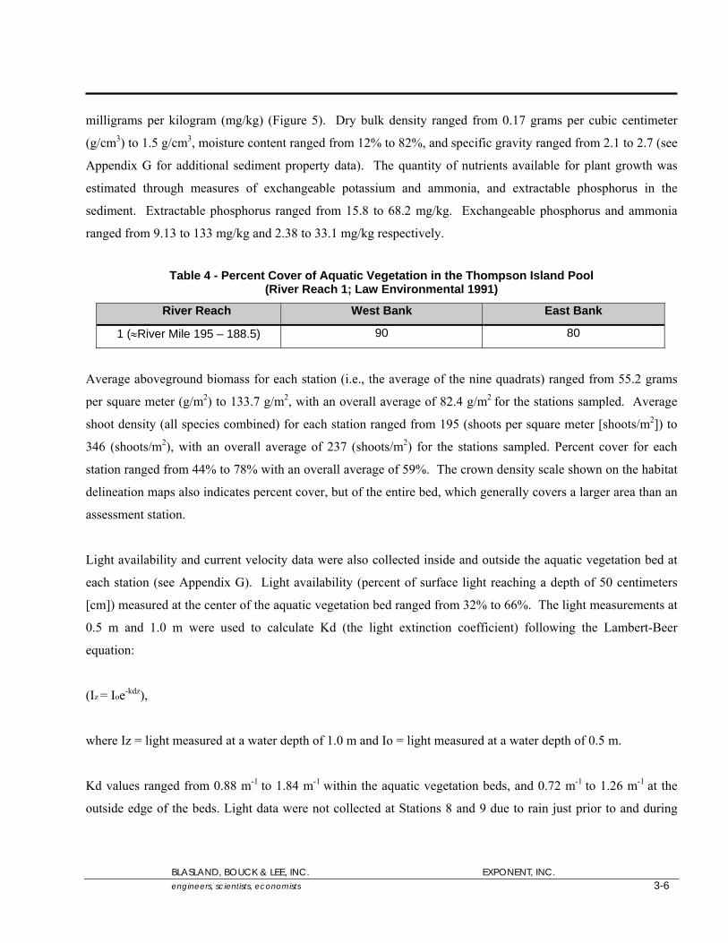
Table 4 - Percent Cover of Aquatic Vegetation in the Thompson Island Pool
(River Reach 1; Law Environmental 1991)
River Reach West Bank East Bank
1 (≈River Mile 195 – 188.5) 90 80
Average aboveground biomass for each station (i.e., the average of the nine quadrats) ranged from 55.2 grams
per square meter (g/m2) to 133.7 g/m2, with an overall average of 82.4 g/m2 for the stations sampled. Average
shoot density (all species combined) for each station ranged from 195 (shoots per square meter [shoots/m2]) to
346 (shoots/m2), with an overall average of 237 (shoots/m2) for the stations sampled. Percent cover for each
station ranged from 44% to 78% with an overall average of 59%. The crown density scale shown on the habitat
delineation maps also indicates percent cover, but of the entire bed, which generally covers a larger area than an
assessment station.
Light availability and current velocity data were also collected inside and outside the aquatic vegetation bed at
each station (see Appendix G). Light availability (percent of surface light reaching a depth of 50 centimeters
[cm]) measured at the center of the aquatic vegetation bed ranged from 32% to 66%. The light measurements at
0.5 m and 1.0 m were used to calculate Kd (the light extinction coefficient) following the Lambert-Beer
equation:
(Iz = Ioe-kdz),
where Iz = light measured at a water depth of 1.0 m and Io = light measured at a water depth of 0.5 m.
Kd values ranged from 0.88 m-1 to 1.84 m-1
within the aquatic vegetation beds, and 0.72 m-1 to 1.26 m-1
at the
outside edge of the beds. Light data were not collected at Stations 8 and 9 due to rain just prior to and during

BLASLAND, BOUCK & LEE, INC. EXPONENT, INC. engineers, scientists, economists 3-7
sampling. These Kd values represent light availability under low flow and low turbidity conditions that existed
during the time of sampling.
Current velocity measurements were collected inside and outside the aquatic vegetation bed at each station (see
Appendix G). Within the aquatic vegetation beds, current velocity ranged from 0.00 to 1.12 feet per second
(fps). At the outside edge of the aquatic vegetation beds, current velocity ranged from 0.06 to 0.86. The highest
current velocity recorded was inside Station 1 located just south of the former Fort Edward Dam. Overall, the
current velocities were lower in the aquatic vegetation bed than current velocities taken immediately outside the
bed on the channel side. However, current velocities were relatively low and showed little variability between
or within stations.
Based on the limited information available from the 2003 sampling (in which only nine of a planned 52 aquatic
vegetation beds were assessed), a Spearman rank correlation matrix was constructed using station averages for
aboveground biomass, stem density, percent cover, adjusted depth, nutrients (K, NH4, PO4), TOC, percent
fines, light attenuation (Kd), and current (Table 5 below). Two significant (p<0.05) correlations were identified
– between stem density and depth and between stem density and K (exchangeable potassium in the sediment).
Table 5 – Significance Levels for Spearman Rank Correlation of Aquatic Vegetation Bed Parameters Biomass No. Stems Cover Depth K NH4 PO4 TOC Fines Kd Current
NoStems 0.971
Cover 0.5233 0.7018
Depth 0.5365 0.0181 0.3715
K 0.4896 0.0242 0.841 0.1905
NH4 0.2301 0.8844 0.3524 0.8844 0.4237
PO4 0.7711 0.3633 0.4329 0.6364 0.0809 0.7435
TOC 0.9062 0.7954 0.465 0.7593 0.3832 0.358 0.465
Fines 0.9436 0.5557 0.6543 0.7954 0.9062 0.4943 0.3108 0.7954
Kd 0.4059 0.3583 0.1751 0.7595 0.088 0.3144 0.0729 0.2742 0.5118
Current 0.0832 0.7845 0.1645 0.8268 0.7984 0.1954 0.282 0.887 0.8128 0.627
The p-value indicates whether the correlation is statistically significant, indicating either a positive or negative
relationship between the two variables. P-values less than 0.05 are considered significant and bolded.

BLASLAND, BOUCK & LEE, INC. EXPONENT, INC. engineers, scientists, economists 3-8
In accordance with the HDA Work Plan, data collected during the assessment of candidate Phase 1 areas was
used to assess the variability between sampling locations and to evaluate whether any modification to the
sampling design was warranted.
Based on an assessment of the variability observed in aboveground biomass, stem density, and percent cover
data for wild celery, the standard error using nine quadrats per station approaches the underlying station-to-
station variability for the stations sampled. Using more than nine quadrats per station would not increase
precision because estimates become dominated by the station-to-station variability. The standard error of
quadrat values at each station was compared to the standard deviation of the station average values (see
Appendix M). Based on nine quadrats, all but one station has less variability within a station than the variability
between station averages for biomass, stem density, and percent cover. Stem density at station 1 has one
anomalous quadrat with a value of 229, whereas the remaining quadrats range from 16 to 85. Variability
estimates excluding that quadrat are well below the station variability. Biomass at station 9 has a few quadrats
with high values as compared to all other quadrats, which increases the variability among quadrats at this
station. However, in order to avoid preferentially weighting small areas higher, an additional sampling station
was added for large aquatic vegetation beds (i.e., greater than 3 acres) in the 2005 sampling. These additional
stations will also provide the flexibility to evaluate variability in characteristics within an aquatic bed. Based on
an evaluation (using standard t-test methods) of the aquatic vegetation data, the current sampling design will
allow detection of 4.7%, 6.9%, and 16.8% reduction in biomass, stem density, and percent cover, respectively.
These percentages are the smallest detectable reduction that the current sampling design would be able to detect,
using a standard t-test. Calculations use a one-sided test for reduction only and an alpha of 0.05, or 95 percent
confidence. Site variability was assumed to be equal to reference variability with nine samples from each area.
This assumption is based on the fact that all stations are currently “reference” stations since no dredging has
occurred. Once the full target and reference dataset is available, this assumption will be tested to ensure that the
most appropriate statistical tests are used for future comparisons. Biomass and stem density were log10 and
square-root transformed, respectively. Percent cover was not transformed. Transformations of biomass and
stem density were done to meet the assumption of normality required by the standard t-test. Evaluations of
normality were done using normal probability plots and Lilliefors goodness of fit tests (See Appendix M). This
level of precision is expected to increase as additional stations are sampled.

BLASLAND, BOUCK & LEE, INC. EXPONENT, INC. engineers, scientists, economists 3-9
Table 6 – Range of Conditions in Aquatic Vegetation Beds in the Upper Hudson River in 2003 (2004 Reassessment Data Are Shown in Brackets.)
Parameter Units Minimum Maximum Mean Standard Deviation
River flow cfs 2,178 3,214 2,898 [6778]
341.31
Total organic carbon mg/kg 990 250,000 26,013 39,593 Percent fines percent 16.4 90.3 68.15 32.42 Dry Bulk Density g/cm3 0.17 1.5 0.93 0.32 Moisture Content percent 12 82 38.0 16.80 Exchangeable phosphorus
mg/l 9.13 133 33.25 [0.94]
12.96
Exchangeable ammonia
mg/l 2.38 33.1 10.77 [0.82]
7.14
Extractable potassium mg/l 15.8 68.2 35.11 [14.2]
26.12
Aboveground biomass g/m2 55.2 133.7 82.34 [70.28]
52.88
Shoot density number/m2 195 346 296.39 [211.56]
200.46
Percent cover percent 44 78 58.35 [52.22]
21.32
Light availability - center of bed
light attenuation coefficient
0.88 1.84 1.2 .40
Current – inside bed (outside bed)
feet per second (fps) 0.00 [0.00] (0.06 [0.07])
1.12 [1.93] (0.86 [0.68])
0.12 [0.31] (0.23 [0.39])
0.29 [0.46] (0.29 [0.25])
Notes: 1. Only one aquatic vegetation bed was reassessed in 2004 and those data are shown in the Mean column. All aquatic vegetation beds
were reassessed for current velocity which allowed calculation of minimum, maximum, mean and standard deviation for that parameter. No light data were taken in 2004 due to rain.
2. Sediment total organic carbon, percent fines, dry bulk density and moisture content were obtained from the SSAP dataset and were not resampled in 2004.
3.3 Shorelines Fourteen shoreline stations (three reference and 11 potential target stations) were assessed between September 8
and September 11, 2003 (see Table 7). Twelve stations were located in River Section 1, and two stations were
located in River Section 2 (see Figures 2 through 4). The dominant inorganic substrate was sand, mixed mostly
with smaller fractions of silt and/or gravel. Only one shoreline station was dominated (100%) by silt (Shoreline
Station 7I). Clay was < 40% of the total sediment composition. Boulders were infrequently observed on
shoreline substrates.

BLASLAND, BOUCK & LEE, INC. EXPONENT, INC. engineers, scientists, economists 3-10
Table 7 – Shoreline Stations for Detailed Functional Assessments
Station Type1 Approximate Location
(RS/RM) Dominant Substrate
Composition Dominant Bank
Composition 1R Reference Upstream from road bridge
across from park on Roger's Island; western shore (above RS1/RM194.4)
Sand/gravel; low cobble/silt mix with trace clay; leafy detritus and muck/mud; woody debris
Stable; optimal vegetation cover2
3R Reference ½ m north of Rt. 4 Bridge; western shore (RS2/RM184)
Sand; low gravel/silt/clay; low leafy detritus; mostly shell hash and trace algae; high woody debris
Stable – unstable; vegetation cover suboptimal or marginal in sections
1 Target ~50 m downstream from railroad trestle bridge at Rogers Island; western shore (RS1/RM194.1)
Sand/silt/clay mix; low leafy detritus with muck/mud; woody debris
Stable; optimal vegetation cover
2 Target Western shore of Roger's Island Boat House; north of south tip (RS1/RM194)
Sand; low silt mix; low leafy detritus with muck/mud; low woody debris
Stable; optimal vegetation cover
3 Target East bank, north of Lock 7, east of Rogers Island (RS1/RM193.9)
Sand; low silt/clay mix; low leafy detritus with muck/mud; woody debris
Moderately stable; optimal vegetation cover
4 Target Eastern shore of Rogers Island, ~300 m north of Lock 7 (RS1RM193.8)
Sand; low gravel/silt mix; low leafy detritus with muck/mud; low woody debris
Moderately stable – Moderately unstable; optimal vegetation cover
2R Target North of GI ~150 m; eastern shore (RS1/RM190.6)
Sand; low gravel and silt; leafy detritus and muck/mud; woody debris
Stable; optimal vegetation cover
5 Target Northeastern shore of GI (RS1/RM190.5)
Gravel; sand/cobble mix; shale; low leafy detritus; woody debris absent
Stable; suboptimal vegetation cover
6 Target Eastern shore, across channel from GI (RS1/RM190.4)
Sand/gravel; low cobble/silt mix; mix of leafy detritus, muck/mud, shell hash; low woody debris
Stable – moderately stable; optimal vegetation cover
7 Target Western shore of GI in the back channel (RS1/RM189.9)
Silt; trace sand/clay; low leafy detritus with muck/mud and vegetation on shore; woody debris
Moderately unstable – optimal vegetation cover
8 Target Eastern shore across from airstrip on GI, just south of riprap bank along road (RS1/RM189.9)
Gravel; cobble/sand and low silt mix; low detritus and muck/mud; mostly shell hash; woody debris
Stable – moderately stable; optimal vegetation cover with suboptimal to marginal area
10 Target Eastern shore of GI, ~500 m north of inlet (RS1/RM189.7)
Sand/silt; low detritus and trace muck/mud; shell hash and sand; woody debris
Stable – moderately unstable; optimal vegetation cover
9 Target 0.3 mile north of Rt. 4 Bridge working western shore (RS2/RM183.9)
Sand/clay; low gravel and silt; low detritus and muck/mud; algae; woody debris
Stable – moderately stable; optimal vegetation cover
11 Target Rt. 4 Bridge, south of wetland (RS2/RM183.6)
Silt; low sand/clay mix low detritus and muck/mud; shell hash and clay/silt; woody debris
Stable – moderately stable; optimal – suboptimal vegetation cover
Notes: 1. Stations are shown in the order that they occur from upriver to downriver locations in the river. The designation of the habitats as
“target” or “reference” is based on a review of proposed dredge area delineations that were in production as working drafts for the Phase 1 DAD Report and is subject to change. For this Phase 1 HA Report, information collected from all natural shoreline habitats is considered “reference” data for the development of the FCIs (see Section 4).
2. Vegetation cover is determined by percent cover of bank vegetation according to Table C.5 in Attachment C.

BLASLAND, BOUCK & LEE, INC. EXPONENT, INC. engineers, scientists, economists 3-11
As shown in Table 8, organic substrate components varied greatly between stations, but at most stations leafy
detritus (range: zero to 60%) and muck/mud (range: zero to 100%) were the most common substrate
components of the shoreline. Small portions of vegetation (< 40%) in the form of an unclassified freshwater alga
were found at some shoreline stations. Another common organic substrate component of the shoreline was large
woody debris (LWD). LWD was most extensive at Shoreline Station 3R in River Section 2, and absent at
Shoreline Station 5I in River Section 1. At the assessed stations, LWD varied in length from 1 to 60 feet, and
was usually less than 1 foot wide.
Table 8 – Range of Conditions Observed in Shorelines in the Upper Hudson River in 2003 (2004 Reassessment Data Are Shown in Brackets.)
Parameter Units Minimum Maximum Mean Standard Deviation
Inorganic Substrate Bedrock percent 0 [0] 0 [0] 0 [0] 0 [0] Boulder percent 0 [0] Trace (<10)
[10] 5 [10] 0 [0]
Cobble percent Trace (<10) [0]
30 [50] 13.3 [30] 8.35 [28.28]
Gravel percent Trace (<10) [0]
70 [100] 28.5 [43] 23.18 [38.99]
Sand percent Trace (<10) [0]
100 [70] 50.6 [49.54]
29.66 [23.71]
Silt percent Trace (<10) [0]
100 [30] 27.7 [22] 27.53 [9.19]
Clay percent Trace (<10) [0]
40 [70] 21.05 [16.67]
12.65 [21.51]
Organic Substrate Detritus percent Trace (<10)
[NA] 40 [NA]
16.6 12.59
Muck-Mud percent Trace (<10) [NA]
100 [NA] 49.5
33.76
Marl percent Trace (<10) [NA]
100 [NA] 81.0
21.32
Vegetated percent Trace (<10) [NA]
40 [NA] 13.4
11.38
Woody Debris Feet Trace (<10) [NA]
60 [NA] 14.44 10.19
Bank Assessment Stable percent Trace (<10)
[0] 100 [100] 74.3 [100] 27.55 [0]
Moderately Stable percent Trace (<10) [0]
90 [100] 43.7 [80] 32.09 [21.38]
Moderately Unstable
percent Trace (<10) [0]
80 [50] 30.6 [32] 27.68 [17.88]
Unstable percent Trace (<10) [0]
0 [0] 0 [0] 0 [0]
Bank Vegetation

BLASLAND, BOUCK & LEE, INC. EXPONENT, INC. engineers, scientists, economists 3-12
Parameter Units Minimum Maximum Mean Standard Deviation
Optimal percent Trace (<10) [0]
100 [100] 90.5 [100] 21.64 [0]
Suboptimal percent Trace (<10) [0]
100 [100] 31.3 [100] 24.75 [0]
Marginal percent Trace (<10) [0]
20 [0] 20.0 [0] 0 [0]
Poor percent Trace (<10) [0]
0 [0] 0 [0] 0 [0]
Riparian Edge Canopy percent Trace (<10)
[20] 100 [90] 55.7 [54.2] 26.2 [25.4]
Understory percent Trace (<10) [Trace]
90 [80] 41.4 [43.7] 25.86 [23.1]
Herbaceous percent 10 [30] 100 [100] 65.2 [76.7] 22.33 [27.1]
Adjacent Landuse None Maintained field
[Residential]
Forested [Forested]
NA NA
Notes: 1. To calculate the mean, the mid-range value was used for the “suboptimal” and “marginal” categories. The resultant mean
value equates to “marginal.” Trace was set to “5” to calculate the mean and standard deviation. 2. In 2004, organic substrate measurements could not be recorded due to elevated water levels at the time of sampling.
In the candidate Phase 1 areas, no natural shoreline banks were found to be completely unstable (i.e., 60% to
100% of the bank visibly eroding), although several stations contained small areas of exposed root mats and/or
sloughing (Appendix G). The majority of natural shoreline banks had visible erosion in less than 30% of the
area assessed. Stability did not appear to be influenced by adjacent land use: forested areas had shorelines that
were as stable as shorelines adjacent to maintained lands.
The dominant canopy, understory, and herbaceous species observed along the riparian edge of the river are
shown in Appendix G. In each of these vegetated “layers,” percent cover ranged from less than 10% to greater
than 90% with minimum station averages of 20% (canopy), 15% (understory), and 43% (herbaceous).
3.4 Riverine Fringing Wetlands Four riverine fringing wetland stations were assessed between September 8 and 11, 2003. Two wetland stations
were located in River Section 1, and two in River Section 2 (Figures 2 through 4). The riverine fringing
wetlands range in size from less than one-tenth acre to 5.65 acres (see HD Report). The riverine fringing
wetlands sampled to date range from 0.12 acres to 0.27 acres, as shown in Table 9. Larger riverine fringing
wetlands and wetlands identified as ESUHs, to the extent that such areas are targeted for dredging and not
BLASLAND, BOUCK & LEE, INC. EXPONENT, INC. engineers, scientists, economists 3-13
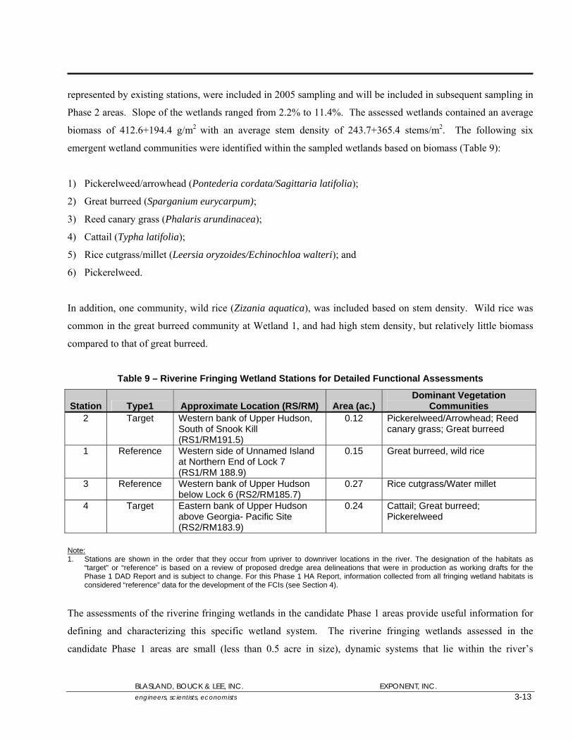
represented by existing stations, were included in 2005 sampling and will be included in subsequent sampling in
Phase 2 areas. Slope of the wetlands ranged from 2.2% to 11.4%. The assessed wetlands contained an average
biomass of 412.6+194.4 g/m2 with an average stem density of 243.7+365.4 stems/m2. The following six
emergent wetland communities were identified within the sampled wetlands based on biomass (Table 9):
1) Pickerelweed/arrowhead (Pontederia cordata/Sagittaria latifolia);
2) Great burreed (Sparganium eurycarpum);
3) Reed canary grass (Phalaris arundinacea);
4) Cattail (Typha latifolia);
5) Rice cutgrass/millet (Leersia oryzoides/Echinochloa walteri); and
6) Pickerelweed.
In addition, one community, wild rice (Zizania aquatica), was included based on stem density. Wild rice was
common in the great burreed community at Wetland 1, and had high stem density, but relatively little biomass
compared to that of great burreed.
Table 9 – Riverine Fringing Wetland Stations for Detailed Functional Assessments
Station Type1 Approximate Location (RS/RM) Area (ac.) Dominant Vegetation
Communities 2 Target Western bank of Upper Hudson,
South of Snook Kill (RS1/RM191.5)
0.12 Pickerelweed/Arrowhead; Reed canary grass; Great burreed
1 Reference Western side of Unnamed Island at Northern End of Lock 7 (RS1/RM 188.9)
0.15 Great burreed, wild rice
3 Reference Western bank of Upper Hudson below Lock 6 (RS2/RM185.7)
0.27 Rice cutgrass/Water millet
4 Target Eastern bank of Upper Hudson above Georgia- Pacific Site (RS2/RM183.9)
0.24 Cattail; Great burreed; Pickerelweed
Note: 1. Stations are shown in the order that they occur from upriver to downriver locations in the river. The designation of the habitats as
“target” or “reference” is based on a review of proposed dredge area delineations that were in production as working drafts for the Phase 1 DAD Report and is subject to change. For this Phase 1 HA Report, information collected from all fringing wetland habitats is considered “reference” data for the development of the FCIs (see Section 4).
The assessments of the riverine fringing wetlands in the candidate Phase 1 areas provide useful information for
defining and characterizing this specific wetland system. The riverine fringing wetlands assessed in the
candidate Phase 1 areas are small (less than 0.5 acre in size), dynamic systems that lie within the river’s

BLASLAND, BOUCK & LEE, INC. EXPONENT, INC. engineers, scientists, economists 3-14
highwater mark during average summer flow conditions (Table 10). Hydrology for these wetlands is primarily
influenced by flow conditions of the Upper Hudson River and its tributaries; minimal hydrologic input is
received from upland sources. Hydrological conditions are dominated by diurnal fluctuations in the river’s
water level created by periodic releases of water from Sacandaga Reservoir. Hydrologic conditions of the
project area are controlled to a lesser extent by other hydroelectric facilities upstream of River Section 1,
episodic flooding due to storm events, tributary input, and seasonal ice flow.
No obvious anthropogenic impacts were noted at Wetland Stations 1, 3, and 4. Wetland Station 2 is bordered by
an adjacent roadway along the upland edge of the wetland.
Table 10 – Range of Conditions Observed in Riverine Fringing Wetlands in the Upper Hudson River in
2003. (2004 Reassessment Data Are Shown in Brackets.)1
Parameter Units Minimum Maximum
Mean Standard Deviation
Size Acre 0.12 0.27 0.19 [0.27] 0.071 Slope Percent 2.2 11.4 6.45 [0.22] 3.80
Biomass g/m2 0.07 783.38 113.56 [26.35]
177.78 [50.62]
Stem Density number/m2 1 1532 80.35
[375.18] 213.5 [609.51]
Percent Contiguous Percent 50 100 87.5 [100] 25 Wetland Edge Feet 324 437 366 [324] 52.12 Note: 1. Only one riverine fringing wetland was reassessed in 2004 and those data are shown in brackets in the Mean column.
The separate quadrat values were used to calculate the mean and standard deviations for biomass and stem density.
3.5 Fish and Wildlife Observations The fish and wildlife species observed during the habitat assessments are shown in Table 11, below. The
completed wildlife observations forms are included in Appendix L.

BLASLAND, BOUCK & LEE, INC. EXPONENT, INC. engineers, scientists, economists 3-15
Table 11 – Fish and Wildlife Species Observed During Habitat Assessments
Species Scientific Name Number Observed Sight/Sign Code Observation
Location Unconsolidated River Bottom
Birds Double-Crested Cormorant
Phalacrocorax auritus
63 Flight UCB-1, UCB-5
Ring Billed Gull Larus delawarensis 16 Flight UCB-3 Mallard Anas platyrhynchos 31 Feeding UCB-1, UCB-4,
UCB-6 Fish
Smallmouth Bass Micropterus dolomieui
8 Foraging UCB-3, UCB-4
American Eel Anguilla rostrata 1 Foraging UCB-1 Aquatic Vegetation Bed
Birds Mallard Anas platyrhynchos 89 Feeding, Resting SAV-2, SAV-3,
SAV-6, SAV-7, SAV-8
Great Blue Heron Ardea herodias 12 Foraging, Flight, Resting
SAV-1, SAV-2, SAV-3, SAV-5, SAV-7, SAV-8
Double-Crested Cormorant
Phalacrocorax auritus
10 Foraging, Flight, Resting
SAV-1, SAV-2, SAV-3, SAV-8
Mammals Beaver Castor canadensis 1 Foraging, Fresh
cuttings SAV-2
Amphibians N. Leopard Frog Rana pipiens 10 Resting SAV-2
Riverine Fringing Wetlands Birds Mallard Anas platyrhynchos 6 Feeding WET-1 Belted Kingfisher Ceryle alcyon 2 Flight, Calling WET-4 Great Blue Heron Ardea herodias 2 Feeding, Tracks WET-2, WET-4 Fish Minnow spp. Not Applicable Numerous Feeding, Swimming WET-1, WET-2,
WET-3, WET-4 Sunfish spp. Lepomis sp. 21+ Swimming,
Foraging WET-1, WET-2
Smallmouth Bass Micropterus dolomieui
4+ Swimming, Foraging
WET-1, WET-2
Mammals Muskrat Ondatra zibethica 6 Tracks WET-2, WET-3,
WET-4 White Tail Deer Odocoileus
virginianus 2 Browse, Feeding WET-1, WET-3
Long Tail Weasel Mustela frenata 1 Tracks WET-1 Amphibians Green Frog Rana clamitans
melanota 29 Resting WET-1, WET-4
N. Leopard Frog Rana pipiens 3 Sight WET-1 Shoreline
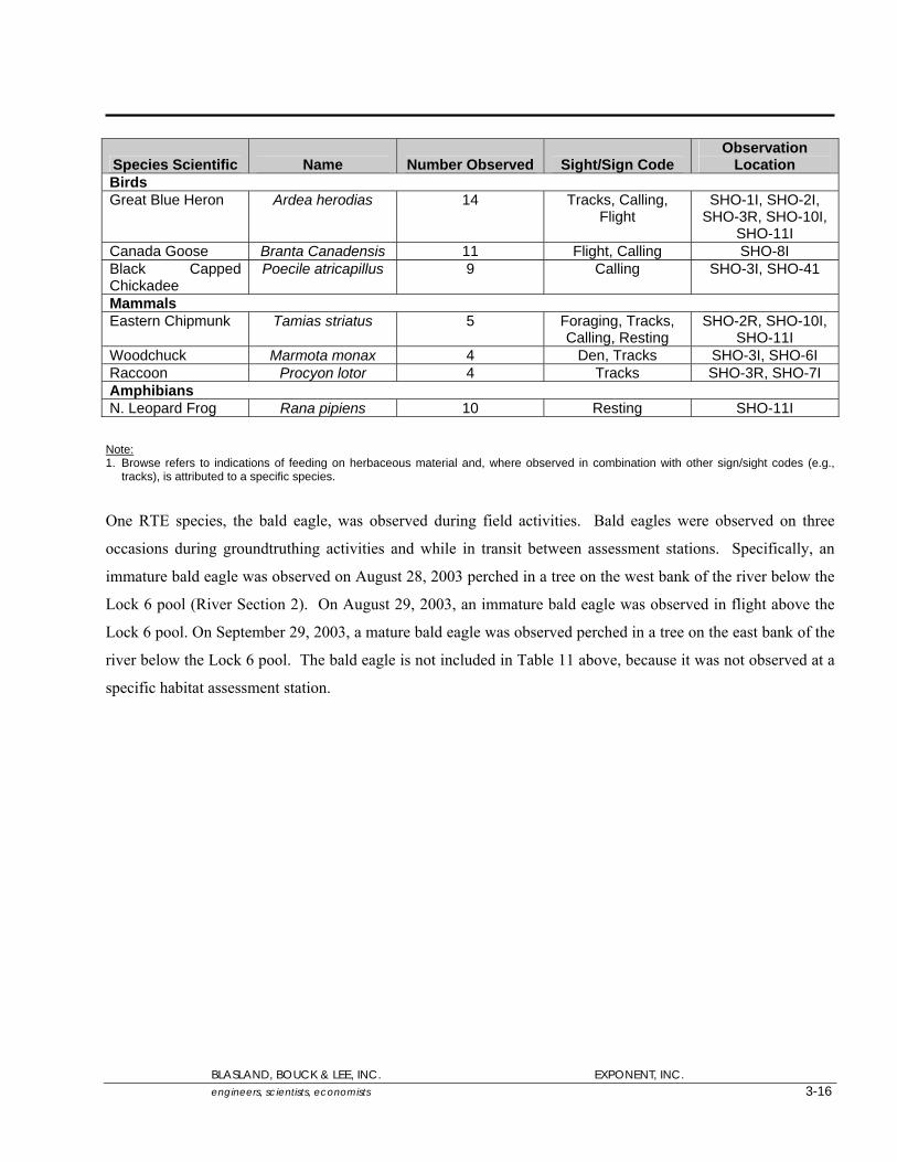
BLASLAND, BOUCK & LEE, INC. EXPONENT, INC. engineers, scientists, economists 3-16
Species Scientific Name Number Observed Sight/Sign Code Observation
Location Birds Great Blue Heron Ardea herodias 14 Tracks, Calling,
Flight SHO-1I, SHO-2I,
SHO-3R, SHO-10I, SHO-11I
Canada Goose Branta Canadensis 11 Flight, Calling SHO-8I Black Capped Chickadee
Poecile atricapillus 9 Calling SHO-3I, SHO-41
Mammals Eastern Chipmunk Tamias striatus 5 Foraging, Tracks,
Calling, Resting SHO-2R, SHO-10I,
SHO-11I Woodchuck Marmota monax 4 Den, Tracks SHO-3I, SHO-6I Raccoon Procyon lotor 4 Tracks SHO-3R, SHO-7I Amphibians N. Leopard Frog Rana pipiens 10 Resting SHO-11I Note: 1. Browse refers to indications of feeding on herbaceous material and, where observed in combination with other sign/sight codes (e.g.,
tracks), is attributed to a specific species.
One RTE species, the bald eagle, was observed during field activities. Bald eagles were observed on three
occasions during groundtruthing activities and while in transit between assessment stations. Specifically, an
immature bald eagle was observed on August 28, 2003 perched in a tree on the west bank of the river below the
Lock 6 pool (River Section 2). On August 29, 2003, an immature bald eagle was observed in flight above the
Lock 6 pool. On September 29, 2003, a mature bald eagle was observed perched in a tree on the east bank of the
river below the Lock 6 pool. The bald eagle is not included in Table 11 above, because it was not observed at a
specific habitat assessment station.
BLASLAND, BOUCK & LEE, INC. EXPONENT, INC. engineers, scientists, economists 4-1
4. FCI Models Functional assessment models, such as FCI models, use a series of measured, recorded, and/or calculated
variables that represent the extent to which selected physical, hydrologic, biological, and sometimes geographic
characteristics of a given site reflect the ability of that site to perform certain ecological functions (Shafer and
Yozzo, 1998). In accordance with the habitat assessment procedures described in the HDA Work Plan, direct
measurements of certain specified physical and biological variables, which were listed in Table 2 of the HDA
Work Plan, are being used to quantify the selected habitat functions. The concept that these types of variables
can be used to quantify habitat functions is one of the foundations of the HGM approach (Shafer and Yozzo,
1998; Ainslie et al., 1999; Smith and Wakeley, 2001; Clairain, 2002) and habitat evaluation procedures (e.g.,
HSIs), and is established in the HDA Work Plan. While these variables consist largely of structural parameters,
some of them can serve as functional parameters as well. For example, the biomass of aquatic vegetation is not
only a structural parameter, but also a functional parameter demonstrating aquatic bed productivity. Similarly,
plant species composition is not only a structural parameter, but also a functional parameter relating to habitat
diversity.
The specific parameters (i.e., the variables defined for the preliminary FCI models) that were initially selected
for measurement in each habitat, as listed in Table 2 of the HDA Work Plan were identified and selected using
four screening criteria (adapted from Shafer and Yozzo, 1998):
a. Presumed importance: There is a documented or hypothesized relationship between the variable and the
function. Potential contribution for describing the function(s) is sufficient to warrant its inclusion in the
model.
b. Basis of importance: Supporting data describe the relationship between the variable and function.
c. Feasibility of measurement: The variable can be easily measured, observed, or recorded at sufficient
resolution for the data to be of use.
d. d. Integrative measurement: The variable is not subject to extreme inter- or intra-annual variability, and/or is
independent of other variables (i.e., does not duplicate another variable).
As noted above, field data were collected from assessment locations within the candidate Phase 1 areas in
September and October 2003 and are presented in Appendix G. Data from the reassessment of a subset of
stations, conducted in September 2004, are presented in Appendix K. The preliminary functions and variables
were then reevaluated to identify variables that warranted inclusion in the current FCI models described below
BLASLAND, BOUCK & LEE, INC. EXPONENT, INC. engineers, scientists, economists 4-2
in this section. The FCI values presented in this section are based solely on the 2003 data. (FCI values
calculated from the 2004 reassessment data are presented in subsection 6.1). If there were insufficient data for a
specific variable, or data were not obtained due to field conditions, the variable(s) was removed from the current
FCI model as described below. However, all variables listed in Table 2 of the HDA Work Plan will be retained
for re-evaluation once remaining Phase 1 and Phase 2 data are available. The mathematical relationships among
variables will also be re-evaluated once the remaining data have been collected.
Collected data have different units and scales. Therefore, all data were transformed into unitless subindices
ranging from 0.0 to 1.0 for integration into the FCI models (Smith and Wakeley, 2001). Appendix H provides
text and graphs showing how these transformations were completed. These graphs show that, for most
variables, the highest measured value is set at 1.0 and that the higher the measured value, the higher the
subindex score (to a maximum of 1.0). However, for several variables (e.g., percent cover of aquatic
vegetation), the subindex score decreases from 1.0 as the measured value increases past a maximum measured
value (equal to a subindex of 1.0). For the purposes of developing the FCI models for the candidate Phase 1
areas, and in accordance with the HDA Work Plan, all stations were considered “reference stations” (since they
represent current, pre-dredging conditions), and a hypothetical “optimal habitat” was developed by combining
the optimal subindex scores from these stations for each of the habitat types. For each of the parameters
measured, a subindex value of 1.0 was assigned to the optimal observed condition – which, in some cases, was
the highest measured value (e.g., for aboveground biomass) and, in some cases, was the lowest measured value
(e.g., for percent nuisance species) – and was used to scale the measured variables. The FCI value for the
hypothetical optimal habitat thus calculates to 1.0. Based on the data collected in 2003, FCI values for the
unconsolidated river bottom range from 0.39 to 0.88, for aquatic vegetation beds from 0.31 to 0.87, for
shorelines from 0.50 to 1.0, and for riverine fringing shoreline wetlands from 0.60 to 0.84. The FCI for each
habitat is habitat-specific and cannot be used for comparisons between habitats to evaluate the success of the
habitat replacement/reconstruction effort. However, comparisons of FCIs among habitat types may be useful to
evaluate changes in habitat types or functions that may result from the remediation project.
Under the habitat replacement and reconstruction program, it is not the goal that the specific pre-dredging FCI
value at each station be attained after dredging. Nor is it the goal of the program to improve overall habitat
conditions of the Upper Hudson River so as to achieve an optimal subindex and/or FCI score of 1.0 at each
station or to reach a higher overall level than recorded at baseline conditions. The goal of the habitat
replacement and reconstruction program is to replace the functions of the habitats of the Upper Hudson River to
within the range of functions found in similar physical settings in the Upper Hudson River, given the changes in
BLASLAND, BOUCK & LEE, INC. EXPONENT, INC. engineers, scientists, economists 4-3
river conditions that will result from remedy implementation or other factors. . This goal will be achieved if the
post-dredging habitat-specific FCI values within impacted areas at an appropriate spatial scale fall within the
range of FCI values in non-impacted areas, accounting for habitat size. The appropriate spatial scale for these
comparisons will be determined by the data and may consist of comparisons on a reach basis or on an overall
river section basis. At some stations, the post-dredging FCI values may be higher than current values (e.g.,
when the amount of nuisance species is reduced), while at other stations the post-dredging FCI values may be
lower than current values. However, the goal will be attained so long as the overall range of values is within the
range at reference areas, with a similar overall habitat value. The specific spatial scale at which post-dredging
habitat-specific FCI values will be compared, and the specific statistical methods to be used in the comparisons,
will be specified in the Adaptive Management Plans. The specific variables and FCI models for the candidate
Phase 1 areas are described in the following subsections.
4.1 Unconsolidated River Bottom As described in the HDA Work Plan, assessing the unconsolidated river bottom habitats consisted of measuring
habitat-specific structural data to represent selected unconsolidated river bottom habitat functions. The
preliminary list of structural data (variables) and associated functions for unconsolidated river bottom habitats is
included in Table 2 of the HDA Work Plan.
An introduction to unconsolidated river bottom and a description of the FCI models based on candidate Phase 1
area data for this habitat are presented below.
4.1.1 Introduction Substrate is one of the most important environmental factors that influence the abundance, composition, and
distribution of infaunal and epifaunal benthic macroinvertebrate (BMI) communities that may reside in
unconsolidated river bottom habitats. Typically, coarse sediments (e.g., cobble, rock, and coarse sand) are
characteristic of substrates in systems of more rapid surface-water flow. Substratum represented by larger
particles or stones is higher in structural complexity and supports a diverse macroinvertebrate community
(Hynes, 1966). BMI species that prefer these habitats include mayflies (Ephemeroptera), stoneflies
(Plecoptera), and caddisflies (Trichoptera) (Merritt and Cummins, 1984). In addition, substrates with larger
particles (e.g., rock/cobble) are used by many species of fish as spawning substrate. For example, smallmouth

BLASLAND, BOUCK & LEE, INC. EXPONENT, INC. engineers, scientists, economists 4-4
bass (Micropterus dolomieu) spawn primarily on rock or gravel beds in rivers and lakes (Sowa and Rabeni,
1995).
Fine sediments (e.g., fine sands and silt) are typically colonized by BMI communities that are tolerant of
reduced-flow conditions. BMI species that prefer fine sediments include opportunistic aquatic earthworms
(Oligochaeta) and midges (Chironomidae) (Merritt and Cummins, 1984). These groups often dominate (or
codominate) invertebrate assemblages in sediments from depositional habitat systems where finer sediments are
often associated with higher TOC. In addition, lower species diversity is typically reported for fish collected
over featureless substrates when compared to habitats containing cobble and/or rubble (Danehy et al., 1991;
Snyder et al., 1996).
4.1.2 FCI Models Based on Candidate Phase 1 Area Data Subsection 3.1 of this Phase 1 HA Report generally describes the data results for unconsolidated river bottom in
the candidate Phase 1 areas. Those descriptions are based on data collected in accordance with the protocols for
assessing unconsolidated river bottom habitats (Appendix A). However, it should be noted that some data were
not collected due to habitat constraints within candidate Phase 1 areas of the river bottom. For example, there
are no “high gradient” areas of the river where embeddedness of substrate features can accurately be assessed.
Therefore, in accordance with the protocols for assessing the unconsolidated river bottom habitats (Appendix
A); substrates were assessed as “pooled” areas. This information was included, as appropriate, into the
development of the FCI models.
After review of the studies listed above, other FCI models (Shafer and Yozzo, 1998; Ainslie et al., 1999; Findlay
et al., 2002), and data from the candidate Phase 1 areas, the following FCI models were developed for the
unconsolidated river bottom habitats in the Upper Hudson River (Table 12, below). The mathematical
relationships between model variables are based on national and regional guidebooks (Shafer and Yozzo, 1998;
Ainslie et al., 1999), local FCI models (Findlay et al., 2002), and professional judgment. These relationships
will be re-evaluated, and revised if necessary, based on the additional data collected and any validation of
assumptions performed in accordance with subsection 6.3.3. (Note that downfall will be added as a variable to
this model, and that the FCI model will be revised once downfall data have been collected.)
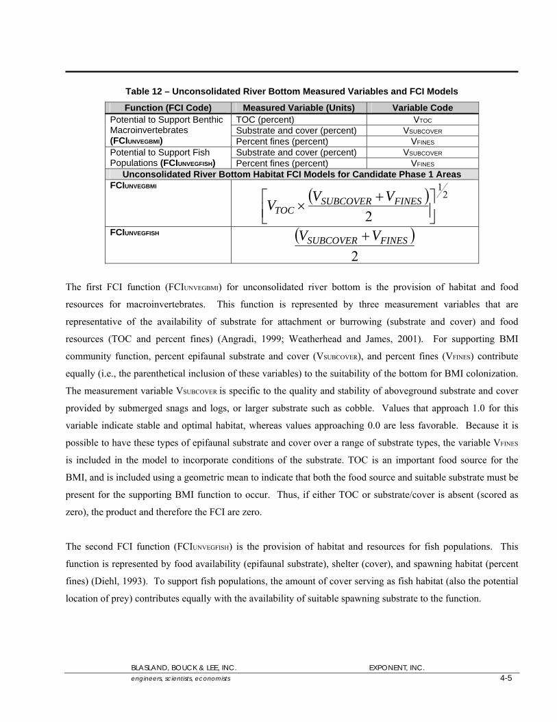
Table 12 – Unconsolidated River Bottom Measured Variables and FCI Models
Function (FCI Code) Measured Variable (Units) Variable Code TOC (percent) VTOC Substrate and cover (percent) VSUBCOVER
Potential to Support Benthic Macroinvertebrates (FCIUNVEGBMI) Percent fines (percent) VFINES
Substrate and cover (percent) VSUBCOVER Potential to Support Fish Populations (FCIUNVEGFISH) Percent fines (percent) VFINES
Unconsolidated River Bottom Habitat FCI Models for Candidate Phase 1 Areas FCIUNVEGBMI
( ) 21
2 ⎥⎦⎤
⎢⎣⎡ +
× FINESSUBCOVERTOC
VVV
FCIUNVEGFISH ( )2
FINESSUBCOVER VV +
The first FCI function (FCIUNVEGBMI) for unconsolidated river bottom is the provision of habitat and food
resources for macroinvertebrates. This function is represented by three measurement variables that are
representative of the availability of substrate for attachment or burrowing (substrate and cover) and food
resources (TOC and percent fines) (Angradi, 1999; Weatherhead and James, 2001). For supporting BMI
community function, percent epifaunal substrate and cover (VSUBCOVER), and percent fines (VFINES) contribute
equally (i.e., the parenthetical inclusion of these variables) to the suitability of the bottom for BMI colonization.
The measurement variable VSUBCOVER is specific to the quality and stability of aboveground substrate and cover
provided by submerged snags and logs, or larger substrate such as cobble. Values that approach 1.0 for this
variable indicate stable and optimal habitat, whereas values approaching 0.0 are less favorable. Because it is
possible to have these types of epifaunal substrate and cover over a range of substrate types, the variable VFINES
is included in the model to incorporate conditions of the substrate. TOC is an important food source for the
BMI, and is included using a geometric mean to indicate that both the food source and suitable substrate must be
present for the supporting BMI function to occur. Thus, if either TOC or substrate/cover is absent (scored as
zero), the product and therefore the FCI are zero.
The second FCI function (FCIUNVEGFISH) is the provision of habitat and resources for fish populations. This
function is represented by food availability (epifaunal substrate), shelter (cover), and spawning habitat (percent
fines) (Diehl, 1993). To support fish populations, the amount of cover serving as fish habitat (also the potential
location of prey) contributes equally with the availability of suitable spawning substrate to the function.
BLASLAND, BOUCK & LEE, INC. EXPONENT, INC. engineers, scientists, economists 4-5
BLASLAND, BOUCK & LEE, INC. EXPONENT, INC. engineers, scientists, economists 4-6
4.2 Aquatic Vegetation Beds As described in the HDA Work Plan, assessing the aquatic vegetation bed habitats consisted of measuring
habitat-specific structural data to represent selected aquatic vegetation bed habitat functions. The preliminary
list of structural data (variables) and associated functions for aquatic vegetation bed habitat is included in Table
2 of the HDA Work Plan.
An introduction to aquatic vegetation beds and a description of the FCI models based on candidate Phase 1 area
data for this habitat are presented below.
4.2.1 Introduction Numerous studies have shown that aquatic vegetation is excellent habitat for fish. Aquatic vegetation
commonly contains large densities of macroinvertebrate prey (Rozas and Odum, 1987; Scott, 1987; Gotceitas
and Colgan, 1987; Bain and Boltz, 1992; Hayse and Wissing, 1996; Randall et al., 1996; Cyr and Downing,
1998) that appear to be present due to the structural “complexity” of the plants (Gerrish and Bristow, 1979). In
addition to food sources, fish find refuge and cover from predation in aquatic vegetation beds (Gotceitas and
Colgan, 1987; Rozas and Odum, 1987; Mittelbach and Osenberg, 1993; Hayse and Wissing, 1996; Randall et
al., 1996). Aquatic vegetation beds may also serve as nursery habitat in rivers for juvenile game fish
(Casselman and Lewis, 1996).
Aquatic vegetation beds increase the structural complexity of shallow water habitats, which has been suggested
by several authors as the reason for increased species richness in these areas (Bain and Boltz, 1992; Randall et
al., 1996). For example, a common species in the Upper Hudson River, largemouth bass (Micropterus
salmoides), is most abundant in areas with vegetation (Jenkins et al., 1952; Miller, 1975) and other forms of
cover (e.g., logs, brush, and debris). Other researchers have suggested that aquatic vegetation beds support
behavioral mechanisms related to foraging strategy or functional biology of a species. The physical presence of
the plant also baffles wave energy, creating a depositional environment and provides sediment stabilization
(Madsen et al., 2001; Koch, 2001). In addition, aquatic vegetation beds mediate nutrient exchange between the
sediments and the overlying water column and have the ability to take-up and retain nutrients from both media
(Carpenter and Lodge, 1986). Many species of aquatic vegetation are able to export DO to the water column,
and there is evidence that the dynamics of the DO may vary among species. In studies conducted in the tidal
portion of the Hudson River, DO measurements varied diurnally and tidally for aquatic vegetation beds
BLASLAND, BOUCK & LEE, INC. EXPONENT, INC. engineers, scientists, economists 4-7
dominated by water chestnut and wild celery, respectively (Caraco and Cole, 2002; Findlay et al., In Review).
Water chestnut DO concentrations measured on the edge of the beds were generally similar to those found in the
river channel (7.0-8.0 milligrams per liter [mg/L]); however, DO concentrations measured within water chestnut
beds with values below 2.5 mg/L up to 40% of the time. DO concentrations measured in wild celery were often
at or above concentrations found in the river channel but did not drop below 5.0 mg/L even during warmer
surface water temperatures.
4.2.2 FCI Models Based on Candidate Phase 1 Area Data Subsection 3.2 of this Phase 1 HA Report generally describes the results from the aquatic vegetation bed habitat
assessment in the candidate Phase 1 areas. Those descriptions are based on data collected in accordance with
the protocols for assessing the aquatic vegetation bed habitats (Appendix B). Some of the data are limited and
are not included in the FCI models presented here. Specifically, the light availability and current velocity data
from the candidate Phase 1 areas were collected late in the growing season for a short time (late September) and
provide limited information on the role that these variables play in determining the functions of aquatic
vegetation bed habitats. The light availability and current velocity variables will be re-considered for inclusion
in the models once remaining Phase 1 and 2 data are collected. However, information on these variables derived
from bathymetric data (related to light availability) and the hydrodynamic model (current velocity) are being
used in the SAV model to be provided in the Adaptive Management Plan. Additionally, plant species
composition (% non-native) is not included in the current calculations because non-native species have not been
sampled to date. The variable will be retained and used, as necessary, following review of the remaining
assessment data.
Similarly, aboveground biomass is an important variable for several functions being assessed, including
supporting fish populations, phytophilous and benthic macroinvertebrate (PMI and BMI, respectively)
populations and nutrient cycling. Initially a separate function, macrophyte primary productivity was identified.
That function is largely represented by biomass (Downing and Anderson, 1985; Mellors, 1991). Therefore, the
macrophyte primary productivity function was removed and aboveground biomass is included, where
appropriate, in the other functional indices for the aquatic vegetation beds. Finally, the variables listed for the
water quality enhancement function in Table 2 of the HDA Work Plan are a subset of those listed for the
stabilization of substrate function. The water quality enhancement function is provided largely by the structure
of the vegetation that baffles wave/current energy to allow particles to settle out of suspension. This function is
also captured in the stabilization of substrate function; thus a separate water quality enhancement function is not

included for the candidate Phase 1 areas. However, it will be retained for re-evaluation following collection of
data from the Phase 2 areas.
After reviewing the studies described above, other FCI models (e.g., Shafer and Yozzo, 1998; Ainslie et al.,
1999; Findlay et al., 2002), the preliminary variable and functions described in the HDA Work Plan, and data
from the candidate Phase 1 areas, the following FCI models were developed for the aquatic vegetation bed
habitats in the Upper Hudson River (Table 13, below). The mathematical relationships between model variables
are based on national and regional guidebooks (Shafer and Yozzo, 1998; Ainslie et al., 1999), local FCI models
(Findlay et al., 2002), and professional judgment. These relationships will be re-evaluated, and revised if
necessary, based on the additional data collected and any validation of assumptions performed in accordance
with subsection 6.3.3. (Note that downfall will be added as a variable to this model, and that the FCI model will
be revised once downfall data have been collected.)
Table 13 – Aquatic Vegetation Bed Habitat Measured Variables and FCI Models
Function (FCI Code) Measured Variable (Units) Variable Code Shoot biomass (g/m2) VSAVBIO
Shoot density (number/m2) VSAVDENSE Plant species composition (% native) VSAVSPP TOC (percent) VSAVTOC
Support PMI/BMI Populations (FCISAVMACROS)
Water depth (cm) VSAVDEPTH Shoot biomass (g/m2) VSAVBIO
Shoot density (number/m2) VSAVDENSE Plant species composition (% native) VSAVSPP TOC (percent) VSAVTOC Water depth (cm) VSAVDEPTH
Provide Habitat for Fish Populations (FCISAVFISH)
Percent cover (percent) VSAVCOVER Shoot density (g/m2) VSAVDENSE Percent fines (percent) VFINES
Stabilization of Substrate (FCISAVSTAB)
Percent cover (percent) VSAVCOVER Shoot biomass (g/m2) VSAVBIO TOC (mg/kg) VSAVTOC
Nutrient Cycling (FCISAVNUTS)
Sediment nutrient availability (mg/kg) VSNN Aquatic Vegetation Bed Habitat FCI Models for Phase 1 Areas
FCISAVMACROS ( )5
SAVDEPTHSAVSPPSAVDENSESAVTOCSAVBIO VVVVV ++++
FCISAVFISH ( )2
SAVCOVERSAVMACROS VFCI +
FCISAVSTAB ( ) 2
1
2 ⎥⎦⎤
⎢⎣⎡ ×
+FINES
SAVCOVERSAVDENSE VVV
BLASLAND, BOUCK & LEE, INC. EXPONENT, INC. engineers, scientists, economists 4-8
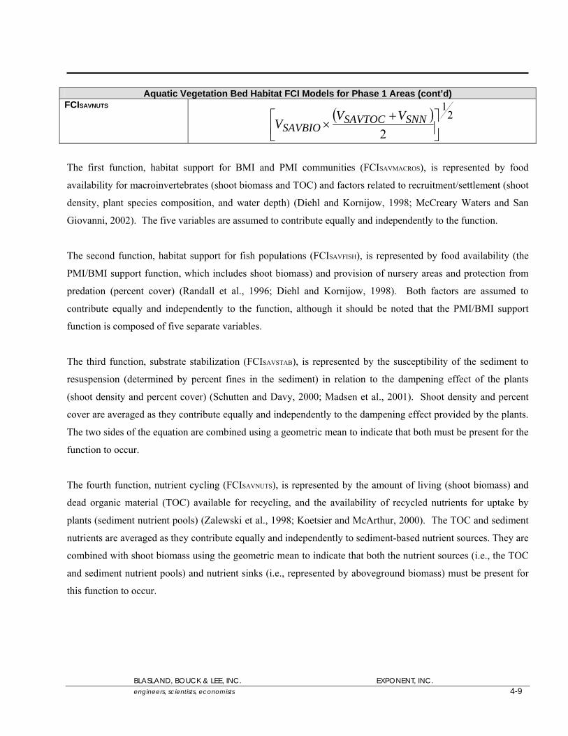
Aquatic Vegetation Bed Habitat FCI Models for Phase 1 Areas (cont’d) FCISAVNUTS
( ) 21
2 ⎥⎦⎤
⎢⎣⎡ +
× SNNSAVTOCSAVBIO
VVV
The first function, habitat support for BMI and PMI communities (FCISAVMACROS), is represented by food
availability for macroinvertebrates (shoot biomass and TOC) and factors related to recruitment/settlement (shoot
density, plant species composition, and water depth) (Diehl and Kornijow, 1998; McCreary Waters and San
Giovanni, 2002). The five variables are assumed to contribute equally and independently to the function.
The second function, habitat support for fish populations (FCISAVFISH), is represented by food availability (the
PMI/BMI support function, which includes shoot biomass) and provision of nursery areas and protection from
predation (percent cover) (Randall et al., 1996; Diehl and Kornijow, 1998). Both factors are assumed to
contribute equally and independently to the function, although it should be noted that the PMI/BMI support
function is composed of five separate variables.
The third function, substrate stabilization (FCISAVSTAB), is represented by the susceptibility of the sediment to
resuspension (determined by percent fines in the sediment) in relation to the dampening effect of the plants
(shoot density and percent cover) (Schutten and Davy, 2000; Madsen et al., 2001). Shoot density and percent
cover are averaged as they contribute equally and independently to the dampening effect provided by the plants.
The two sides of the equation are combined using a geometric mean to indicate that both must be present for the
function to occur.
The fourth function, nutrient cycling (FCISAVNUTS), is represented by the amount of living (shoot biomass) and
dead organic material (TOC) available for recycling, and the availability of recycled nutrients for uptake by
plants (sediment nutrient pools) (Zalewski et al., 1998; Koetsier and McArthur, 2000). The TOC and sediment
nutrients are averaged as they contribute equally and independently to sediment-based nutrient sources. They are
combined with shoot biomass using the geometric mean to indicate that both the nutrient sources (i.e., the TOC
and sediment nutrient pools) and nutrient sinks (i.e., represented by aboveground biomass) must be present for
this function to occur.
BLASLAND, BOUCK & LEE, INC. EXPONENT, INC. engineers, scientists, economists 4-9
BLASLAND, BOUCK & LEE, INC. EXPONENT, INC. engineers, scientists, economists 4-10
4.3 Shorelines As described in the HDA Work Plan, assessing the shoreline habitats consisted of measuring habitat-specific
structural data to represent selected shoreline habitat functions. The preliminary list of structural data
(variables) and associated functions for shoreline habitat is included in Table 2 of the HDA Work Plan. A brief
introduction to shorelines and a description of the FCI models based on candidate Phase 1 area data for this
habitat are presented below.
4.3.1 Introduction Natural shorelines with an extensive riparian canopy serve many functions. An established canopy provides
shade and cover, which can minimize daily and seasonal temperature fluctuations and keeps temperatures
relatively cool (Hunter, 1991; Sowa and Rabeni, 1995). Deadfall (e.g., fallen and submerged trees) and
vegetation may provide spawning habitat and cover for many types of aquatic organisms (Herman et al., 1964;
Ward and Robinson, 1974; Kitchell et al., 1977; Helfman, 1979; Hunter, 1991). For shorelines in candidate
Phase 1 areas, the composition of the organic substrate, bank stability, and range of vegetation cover in the
canopy, understory, and herbaceous layers are described in more detail in subsection 3.3 (see also Appendix G
for station-specific values).
4.3.2 FCI Models Based on Candidate Phase 1 Area Data Subsection 3.3 of this Phase 1 HA Report generally describes the data results for shoreline habitats in the
candidate Phase 1 areas. These descriptions are based on data that were collected using methods described in
the protocols for assessing shoreline habitats (Appendix C).
During the conceptual development of selecting measured variables for shoreline stability function, downfall
was thought to provide an “armoring” effect against high flows. Downfall, such as layered tree revetments or
root wads, is often used in this manner to aid in shoreline replacement and reconstruction, but along natural
shorelines where it is patchily distributed, downfall can also be associated with unstable bank conditions.
Because downfall may be interpreted as both an indicator of bank stability or instability along natural shorelines,
it was removed as a variable from the shoreline stability FCI model.
Clearly, many of the functions provided by natural shorelines are based, at a minimum, on the existence of
sufficient bank stability and vegetation to provide cover, shade, and habitat for fish and wildlife. Thus, the
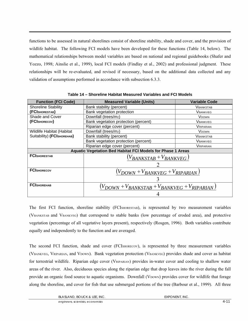
functions to be assessed in natural shorelines consist of shoreline stability, shade and cover, and the provision of
wildlife habitat. The following FCI models have been developed for these functions (Table 14, below). The
mathematical relationships between model variables are based on national and regional guidebooks (Shafer and
Yozzo, 1998; Ainslie et al., 1999), local FCI models (Findlay et al., 2002) and professional judgment. These
relationships will be re-evaluated, and revised if necessary, based on the additional data collected and any
validation of assumptions performed in accordance with subsection 6.3.3.
Table 14 – Shoreline Habitat Measured Variables and FCI Models
Function (FCI Code) Measured Variable (Units) Variable Code Bank stability (percent) VBANKSTAB Shoreline Stability
(FCISHORESTAB) Bank vegetation protection VBANKVEG Downfall (trees/m2) VDOWN
Bank vegetation protection (percent) VBANKVEG Shade and Cover (FCISHORECOV)
Riparian edge cover (percent) VRIPARIAN Downfall (trees/m2) VDOWN Bank stability (percent) VBANKSTAB Bank vegetation protection (percent) VBANKVEG
Wildlife Habitat (Habitat Suitability) (FCISHOREHAB)
Riparian edge cover (percent) VRIPARIAN Aquatic Vegetation Bed Habitat FCI Models for Phase 1 Areas
FCISHORESTAB ( )2
BANKVEGBANKSTAB VV +
FCISHORECOV ( )3
RIPARIANBANKVEGDOWN VVV ++
FCISHOREHAB ( )4
RIPARIANBANKVEGBANKSTABDOWN VVVV +++
The first FCI function, shoreline stability (FCISHORESTAB), is represented by two measurement variables
(VBANKSTAB and VBANKVEG) that correspond to stable banks (low percentage of eroded area), and protective
vegetation (percentage of all vegetative layers present), respectively (Rosgen, 1996). Both variables contribute
equally and independently to the function and are averaged.
The second FCI function, shade and cover (FCISHORECOV), is represented by three measurement variables
(VBANKVEG, VRIPARIAN, and VDOWN). Bank vegetation protection (VBANKVEG) provides shade and cover as habitat
for terrestrial wildlife. Riparian edge cover (VRIPARIAN) provides in-water cover and cooling to shallow water
areas of the river. Also, deciduous species along the riparian edge that drop leaves into the river during the fall
provide an organic food source to aquatic organisms. Downfall (VDOWN) provides cover for wildlife that forage
along the shoreline, and cover for fish that use submerged portions of the tree (Barbour et al., 1999). All three
BLASLAND, BOUCK & LEE, INC. EXPONENT, INC. engineers, scientists, economists 4-11

BLASLAND, BOUCK & LEE, INC. EXPONENT, INC. engineers, scientists, economists 4-12
variables contribute equally and independently to the function and are therefore averaged. The third FCI
function, wildlife habitat suitability (FCISHOREHAB), depends on the nature and type of vegetation present
(downfall, riparian vegetation, bank vegetation) and stability of the habitat (bank stability) (Barbour et al.,
1999). All four variables contribute equally and independently to the function and are therefore averaged.
4.4 Riverine Fringing Wetlands As described in the HDA Work Plan, assessments for the riverine fringing wetland habitats consisted of
measuring habitat-specific structural data to represent selected fringing wetland habitat functions. The
preliminary list of structural data (variables) and associated functions for fringing wetland habitats is included in
Table 2 of the HDA Work Plan. A brief introduction to riverine fringing wetlands and a description of the FCI
models based on candidate Phase 1 area data for this habitat are presented below.
4.4.1 Introduction Wetlands in the Upper Hudson River that could potentially be impacted by remediation activities are relatively
small, fringing, emergent wetlands. A new HGM subclass of “riverine fringing” wetlands has been used to
classify the Hudson River wetlands. Riverine fringing wetlands possess characteristics similar to traditional
HGM classes of riverine and tidal fringe, but riverine fringing wetlands have a unique combination of HGM
setting and hydrodynamics. Benches or slopes inside the river banks provide the HGM setting for riverine
fringing wetlands, and within-channel flow is the dominant water source. Hydrodynamics have both vertical and
horizontal components. The vertical component results from seasonal changes in precipitation and
evapotranspiration in the watershed and episodic changes due to hydrofacilities on the river. The horizontal
component results from non-tidal river flow.
Brazner and Magnuson (1994) found higher fish species diversity and abundance in wetlands adjacent to
undeveloped land, as opposed to wetlands near sandy beaches and developed lands. Based on their HGM
setting and vegetation community, these fringing wetlands are expected to provide a variety of hydrologic,
biogeochemical, and habitat functions. Because riverine fringing wetlands of the Upper Hudson River possess
characteristics common to both riverine wetlands, as described by Ainslie et al. (1999) and Brinson et al. (1995),
and tidal fringing wetlands, as described by Shaffer and Yozzo (1998), the riverine fringing wetlands will
provide some of the functions found in each.

BLASLAND, BOUCK & LEE, INC. EXPONENT, INC. engineers, scientists, economists 4-13
4.4.2 FCI Models Based on Candidate Phase 1 Area Data Subsection 3.4 of this Phase 1 HA Report generally describes the data results for riverine fringing wetland
habitats in the candidate Phase 1 areas. These descriptions are based on data that were collected using methods
described in the protocols for assessing riverine fringing wetland habitats (Appendix D).
The riverine fringing wetlands found within the Upper Hudson River range in size from one-tenth acre to 5.65
acres, but are predominantly small (less than 0.5 acre in size), dynamic systems that lie within the river’s
highwater level under normal flow conditions. Changes in water levels and scouring by ice flows likely impede
the development of shrub-land and forested vegetative communities within the fringing wetland area. Scouring
of the sediment and vegetation by annual ice flow is likely a major factor in developing the dynamic
characteristics of these wetlands and has been documented as a major factor in limiting the diversity of habitats
and preventing the development of shrub and tree communities (Stromberg et al., 1997). Permanently flooded
conditions in the wetlands may also contribute to the limited development of shrub and tree communities, as few
woody species are able to adapt to such conditions in this region. As a result, the fringing wetlands of the Upper
Hudson River are dominated by emergent wetland species. Due to the position of these fringing wetlands in
relation to, and the hydrologic influence of, the Upper Hudson River, soils present in these wetlands are alluvial
and do not possess true O or A horizons (see Appendix J), redoximorphic features, or indicators of a fluctuating
water table. As such, data for these variables could not be collected from the candidate Phase 1 areas. Data
could also not be collected for the interior core area variable due to the small width of most Phase 1 wetlands. In
accordance with the HDA Work Plan, the wetlands must be at least 100 meters wide and of similar length to
allow for this information to be collected.
The three preliminary functions (listed in Table 2 of the HDA Work Plan) that depended on the soil property
variables (export organic carbon, nutrient cycling, and remove and hold elements and compounds) were
reevaluated and combined to provide a function (nutrient and organic cycling) related to the ability of the
wetland to import and/or export nutrients and organic carbon. Additionally, due to the small size and dynamic
nature of the fringing wetlands, primary production may not be a significant function of these wetlands per se.
However, primary production, represented by aboveground biomass, is an important component of several
functions such as energy dissipation and nutrient and organic cycling (Shafer and Yozzo, 1998). Therefore,
aboveground biomass has been included as a variable in those functions where appropriate and a separate
function for primary production is not included for the candidate Phase 1 areas. However, each of the

preliminary functions listed in Table 2 of the HDA Work Plan will be retained for re-evaluation following
collection of data from the remaining Phase 1 and Phase 2 areas.
After review of the studies described above, other FCI models (e.g., Shafer and Yozzo, 1998; Ainslie et al.,
1999; Findlay et al., 2002), the preliminary variable and functions described in the HDA Work Plan, and data
from the candidate Phase 1 areas, the following FCI models were developed for the fringing wetland habitats in
the Upper Hudson River (Table 15, below). The mathematical relationships between model variables are based
on national and regional guidebooks (Shafer and Yozzo, 1998; Ainslie et al., 1999), local FCI models (Findlay
et al., 2002), and professional judgment. These relationships will be re-evaluated, and revised if necessary,
based on the additional data collected and any validation of assumptions performed in accordance with
subsection 6.3.3. (Note that downfall will be added as a variable to this model, and that the FCI model will be
revised once downfall data have been collected.)
Table 15 – Wetland Habitat Measured Variables and FCI Models
Function (FCI Code) Measured Variable (Units) Variable Code Wetland Edge (m) VWETEDGE
Stem density (number/m2) VWETDENSE
Surface-Water Exchange (FCIWATEREX)
Slope (percent) VWETSLOPE
Wetland Edge (m) VWETEDGE
Slope (percent) VWETSLOPE
Stem density (number/m2) VWETDENSE
Stem thickness (mm) VWETTHICK
Energy Dissipation (FCIED)
Stem length (cm) VWETLENGTH
Aboveground biomass (g/m2) VWETBIO
Stem length (cm) VWETLENGTH
Stem thickness (mm) VWETTHICK
Stem density (number/m2) VWETDENSE
Wetland Edge (m) VWETEDGE
Nutrient and Organic Cycling (FCIWETCYCLING)
Slope (percent) VWETSLOPE
Plant species composition (percent) VWETSPP Maintain Character Plant Community (FCIMAINTAINSPP) Nuisance species (percent) VWETNUISANCE
Wetland Edge (m) VWETEDGE
Contiguous with other habitats (percent) VCONTIG
Plant species composition (percent) VWETSPP
Wildlife Habitat (habitat suitability) (FCIWETHAB)
Stem density (number/m2) VWETDENSE Wetland Habitat FCI Models for Candidate Phase 1 Areas
FCIWATEREX ( )3
WETDENSEWETSLOPEWETEDGE VVV ++
FCIED
( ) 21
2 ⎥⎦⎤
⎢⎣⎡ +
× WETTHICKWETLENGTHWATEREX
VVFCI
BLASLAND, BOUCK & LEE, INC. EXPONENT, INC. engineers, scientists, economists 4-14
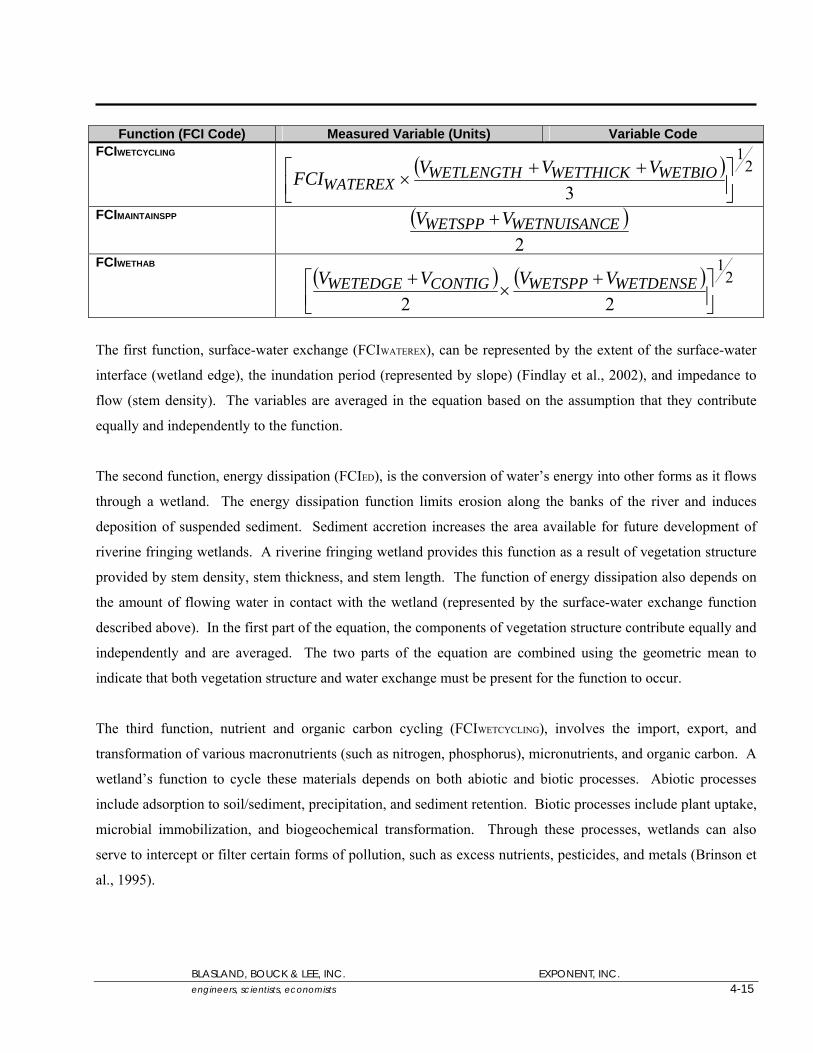
Function (FCI Code) Measured Variable (Units) Variable Code FCIWETCYCLING
( ) 21
3 ⎥⎦⎤
⎢⎣⎡ ++
× WETBIOWETTHICKWETLENGTHWATEREX
VVVFCI
FCIMAINTAINSPP ( )2
EWETNUISANCWETSPP VV +
FCIWETHAB ( ) ( ) 2
1
22 ⎥⎦⎤
⎢⎣⎡ +
×+ WETDENSEWETSPPCONTIGWETEDGE VVVV
The first function, surface-water exchange (FCIWATEREX), can be represented by the extent of the surface-water
interface (wetland edge), the inundation period (represented by slope) (Findlay et al., 2002), and impedance to
flow (stem density). The variables are averaged in the equation based on the assumption that they contribute
equally and independently to the function.
The second function, energy dissipation (FCIED), is the conversion of water’s energy into other forms as it flows
through a wetland. The energy dissipation function limits erosion along the banks of the river and induces
deposition of suspended sediment. Sediment accretion increases the area available for future development of
riverine fringing wetlands. A riverine fringing wetland provides this function as a result of vegetation structure
provided by stem density, stem thickness, and stem length. The function of energy dissipation also depends on
the amount of flowing water in contact with the wetland (represented by the surface-water exchange function
described above). In the first part of the equation, the components of vegetation structure contribute equally and
independently and are averaged. The two parts of the equation are combined using the geometric mean to
indicate that both vegetation structure and water exchange must be present for the function to occur.
The third function, nutrient and organic carbon cycling (FCIWETCYCLING), involves the import, export, and
transformation of various macronutrients (such as nitrogen, phosphorus), micronutrients, and organic carbon. A
wetland’s function to cycle these materials depends on both abiotic and biotic processes. Abiotic processes
include adsorption to soil/sediment, precipitation, and sediment retention. Biotic processes include plant uptake,
microbial immobilization, and biogeochemical transformation. Through these processes, wetlands can also
serve to intercept or filter certain forms of pollution, such as excess nutrients, pesticides, and metals (Brinson et
al., 1995).
BLASLAND, BOUCK & LEE, INC. EXPONENT, INC. engineers, scientists, economists 4-15
BLASLAND, BOUCK & LEE, INC. EXPONENT, INC. engineers, scientists, economists 4-16
Due to the dynamic nature of riverine fringing wetland habitats, the substrate tends to be more variable in
organic and inorganic content than the substrate of depositional wetlands. Thus, the substrate is relatively
devoid of adsorption sites associated with clays and organic matter. For this reason, the nutrient and organic
carbon cycling function primarily depends on biological and hydrological wetland characteristics. Surface-
water exchange (FCIWATEREX) drives nutrient and organic carbon cycling by allowing interaction between the
wetland edge and river flow. Nutrient and organic carbon cycling is proportional to the size of the vegetation
community (aboveground biomass, stem length, stem thickness) because vegetation provides surface area for
microbial populations, which play a large role in cycling, and influences the quantity of detritus produced
(Shafer and Yozzo, 1998). For the second part of the equation, the components of the vegetation community
contribute equally and independently and are averaged. The two parts of the equation are combined using the
geometric mean to indicate that both vegetation community and water exchange must be present for the function
to occur.
The fourth function, maintenance of characteristic plant community (FCIMAINTAINSPP), is related to the ability of
the wetland to provide characteristic species composition (plant species composition). This function generally
decreases when exotic or invasive species comprise a higher proportion of plants present (nuisance species).
Both variables contribute equally and independently to the function and are averaged. The wetland plant
community is critical to the provision of many wetland functions and values, such as maintaining biodiversity,
improving water quality, stabilizing beds/banks, cycling nutrients, and providing habitat (Brinson et al., 1995;
Shafer and Yozzo, 1998).
The fifth function, wildlife habitat (FCIWETHAB), is the potential use by resident and migratory invertebrates,
avifauna, herptofauna, nekton, and mammals. Wetland habitat can also be important to terrestrial wildlife due to
trophic links or cohabitation between upland and wetland areas (Shafer and Yozzo, 1998). Thus, the wildlife
habitat function depends on the structure and composition of the vegetation community (plant species
composition, stem density), the size of the wetland interface with the river (wetland edge), and connectivity
between upland and wetland areas (contiguous with other habitats). The two parts of the equation are combined
using the geometric mean to indicate that both contiguous habitats and the vegetation community must be
present for the function to occur.
BLASLAND, BOUCK & LEE, INC. EXPONENT, INC. engineers, scientists, economists 4-17
4.5 Current Status and Future Use of FCI Models The transformation of the field data to the unitless subindices for each of the variables included in the habitat-
specific FCI models described in the preceding sections is detailed in Appendix H. That appendix also contains
figures depicting the output of the transformation process for each of these variables. As noted above and
discussed in Appendix H, a value of 1.0 has been assigned to the optimal measured value for each parameter
among all stations, and was then used to scale the values for that parameter at all other stations. As a result, the
optimal FCI score for a given station is a hypothetical value of 1.0, but most stations have lower FCI values.
The current, preliminary FCI value for each function and habitat is shown in Table 16, below. It is important to
note that the FCI models and the mathematical relationships for each model are preliminary. Once data have
been collected from all Phase 1 and Phase 2 areas, the subindices and FCIs will be revised using the entire site-
specific data set (Clairain, 2002). At that time, the subindices for the all stations will be revised using the
“optimal” conditions from reference stations as the “1.0” value for each habitat. It should be noted that FCI
values are habitat-specific. For example, although unconsolidated bottom may have a higher mean FCI for the
potential to support fish populations than aquatic vegetation beds have for providing habitat for fish populations,
the value of unconsolidated bottom to fish populations cannot be said to greater than or equal to that of aquatic
vegetation beds. While direct comparison of different habitat types cannot be done to evaluate the success of
the habitat replacement/reconstruction effort, such comparisons may be useful to evaluate changes in habitat
types and functions that may result from the remediation project.
Additional site-specific data may be necessary to support the full development of the FCI model equations for
the Upper Hudson River. Additional data needs for the FCI models are discussed in subsection 6.3.3 below.

BLASLAND, BOUCK & LEE, INC. EXPONENT, INC. engineers, scientists, economists 4-18
Table 16 – Calculated FCI Values for Phase 1 Areas
Unconsolidated River Bottom Potential to Support Macroinvertebrates
Potential to Support Fish Populations
Station FCIUNVEGBMI FCIUNVEGFISH
UCB-1 0.39 0.88 UCB-2 0.88 0.77 UCB-3 0.49 0.82 UCB-4 0.41 0.74 UCB-5 0.48 0.55 UCB-6 0.81 0.70
Aquatic Vegetation Bed Support PMI/BMI
Populations Fish and
Wildlife HabitatStabilization of
Substrate Nutrient Cycling
Station FCISAVMACROS FCISAVFISH FCISAVSTAB FCISAVNUTS
SAV-1 0.75 0.67 0.34 0.67 SAV-2 0.51 0.53 0.59 0.40 SAV-3 0.54 0.59 0.35 0.40 SAV-4 0.62 0.62 0.32 0.50 SAV-5 0.51 0.68 0.47 0.33 SAV-6 0.74 0.87 0.47 0.63 SAV-7 0.52 0.73 0.57 0.42 SAV-8 0.62 0.73 0.31 0.51 SAV-9 0.68 0.68 0.55 0.68
Shoreline Shoreline Stability Shade and Cover Wildlife Habitat Station FCISHORESTAB FCISHORECOV FCISHOREHAB
1R 0.96 0.56 0.65 1I 1 0.53 0.65 2I 0.83 0.46 0.59 2R 0.99 0.55 0.66 3I 0.96 0.61 0.69 3R 0.93 0.85 0.86 4I 0.95 0.57 0.65 5I 0.95 0.56 0.67 6I 1 0.57 0.68 7I 0.88 0.61 0.65 8I 0.97 0.5 0.62 9I 0.99 0.57 0.67
10I 0.97 0.57 0.66 11I 0.97 0.58 0.68
Wetland Surface-water
Exchange Energy
Dissipation
Nutrient and Organic Cycling
Maintain Character
Plant Community
Wildlife Habitat
Station FCIWATEREX FCIED FCIWETCYCLING FCIMAINTAINSPP FCIWETHAB
1 0.74 0.65 0.62 0.82 0.78 2 0.83 0.84 0.83 0.60 0.66 3 0.76 0.61 0.64 0.65 0.60 4 0.74 0.75 0.74 0.76 0.71
BLASLAND, BOUCK & LEE, INC. EXPONENT, INC. engineers, scientists, economists 4-19
4.6 Success Criteria for Habitat Replacement and Reconstruction As stated in the HDA Work Plan, “[t]he primary goal of the habitat program is to replace the functions of the
habitats of the Upper Hudson River to within the range of functions found in similar physical settings in the
Upper Hudson River, in light of the changes in river hydrology, bathymetry, and geomorphology that will result
from the implementation of the USEPA-selected remedy and from possible independent environmental changes
that may occur from other factors” (page 1-2). In accordance with the HDA Work Plan, the range of functions
found in the Upper Hudson River is being assessed through measurement of certain specified variables (listed in
Table 2 of the HDA Work Plan) in the four habitat types during remedial design. As noted above, these
variables consist largely of structural parameters, but also include some functional parameters. That program
will establish the range of these habitat-specific parameters in the Upper Hudson River habitats prior to
dredging, by measuring those parameters both in areas that will be directly impacted by dredging and those that
will not. Based on those data, the specific parameters to be used as design criteria for the habitat replacement
and reconstruction program will be selected to achieve the above objective. Further, these data will be used to
develop “bounds of expectation” for the replaced and reconstructed habitats for use in design, and a suite of
adaptive management techniques will be identified for use in the long-term monitoring and adaptive
management program. The design criteria will be included in the Adaptive Management Plan, which will be
part of the Final Design Report for each phase of dredging.
Success criteria for each habitat type will be developed based on the range of conditions found in reference
areas. This range of conditions defines the “bounds of expectation” for habitat replacement and reconstruction.
Bounds of expectation and success criteria will be developed for:
• Conditions within specific habitats (e.g., an area anticipated to be replaced as unconsolidated river bottom
will be expected to have sediment with grain size falling within the range of grain sizes defined by reference
sites); and
• The overall distribution of habitat types and functions, taking habitat size into consideration, over each
River Section or reach (i.e., for each River Section or reach, the mosaic of post remediation habitats will be
expected to fall within the range of habitats supported by areas of similar physical conditions, such as water
depth, flow, substrate, bank conformation, etc., as in reference areas).
BLASLAND, BOUCK & LEE, INC. EXPONENT, INC. engineers, scientists, economists 4-20
For riverine fringing wetlands unavoidably lost or adversely affected by the dredging project, the goal is to
replace the functions provided by those wetlands, i.e., no net loss of functions. Functional replacement of
riverine fringing wetlands will be accomplished by the replacement of the riverine fringing wetlands in their
original locations, to the extent practicable and appropriate, consistent with the remedy. For locations where it
is not practicable or appropriate to replace the wetland in its original location, and where it is determined
appropriate by USEPA to do so, additional mitigation activities will be undertaken in other dredge areas to
replace the lost function of that wetland.
For submerged aquatic vegetation (SAV) beds, the replacement of SAV beds will be dictated by the post-
dredging river bathymetry (depth) and other factors that control the occurrence of SAV beds (e.g., current
velocity, light availability) within the project area. Where water depths and controlling factors support the
replacement of SAV beds, the goal is to replace those beds. Consistent with agreements between GE and
USEPA, areas in the project area that supported SAV beds prior to dredging and backfilling will be evaluated to
determine if the resulting water depth has increased to a point where these beds would no longer be supported.
These areas will be evaluated to determine if placement of additional backfill would reduce the water depth so
that SAV beds would be supported. Additional backfill, up to 15% of the total volume estimated during design
to be placed as part of the entire project (1 foot over all dredge areas), will be allocated for creation of aquatic
vegetation beds.
As stated in the HDA Work Plan, monitoring of the reference areas after the completion of the remediation will
allow for modifications of the “bounds of expectation” for the measured parameters. Post-dredging comparisons
of those parameters in the dredged areas to those in the reference area data set (i.e., parameters measurements
taken in non-target areas before and after dredging, and in target areas before dredging) will provide the primary
basis for judging the success of the habitat replacement and reconstruction program. The specific parameter
measurements taken for each habitat type will be used to develop FCIs for the relevant functions for that habitat
(as listed in Table 2 of the HDA Work Plan). The habitat replacement and reconstruction program will be
designed to return the overall distribution of the relevant FCI parameters within the dredged areas to be similar
to the overall distribution of such parameters in the habitat-specific reference areas, accounting for habitat size.
It is anticipated that comparisons of the range of conditions in reference and remediated areas will be made by
statistical tests appropriate for the collected data. A “spatially-weighted average” and use of negative null
hypotheses are possible techniques that will be considered. The appropriate spatial scale for these comparisons
will be determined by the data, and may consist of comparisons on a reach basis or on an overall river section
basis. The spatial scale for these comparisons and the specific statistical techniques to be used in the
BLASLAND, BOUCK & LEE, INC. EXPONENT, INC. engineers, scientists, economists 4-21
comparisons will be included in the Adaptive Management Plan, which will be part of the Final Design Report,
for each phase of dredging.
In addition to the site-specific FCI models, HSI models will be used to quantify the fish and wildlife habitat
functions for the species listed in Section 5 below. The HSI models will be used for this purpose in conjunction
with the FCI models, as many of the input parameters are not independent of the FCI variables.
When parameter(s) from target areas within an appropriate spatial scale (e.g., river section or reach) are within
the range of parameter(s) from reference areas (considering overall distribution of values within habitats and
within the relevant river section or reach) for a specific habitat type, the habitat replacement/reconstruction
within those target areas will be considered successful. Given the changes in river conditions that will result
from the dredging, the objective for a specific dredged area cannot be established a priori as either the “low end”
or the “high end” of the range, since physical conditions in each area will determine where the post-dredging
habitat falls within these bounds. A mix of habitats will be established, taking account of physical conditions in
the post-remediation environment, and that habitat mix will be evaluated against the mix of habitats in reference
sites with similar physical conditions. The evaluation of success will be made for each habitat type and will be
based on comparing the overall distribution of the relevant parameters from the dredged areas within a given
spatial extent of the river to the overall distribution of such parameters in the pertinent reference areas, using
appropriate statistical tests. The specific spatial extent (scale) at which post-dredging FCI values will be
compared, and the specific statistical methods to be used in the comparisons, will be specified in the Adaptive
Management Plans that will accompany the Final Design Reports.
FCIs and HSIs will be calculated directly from parameters in both target and reference stations to evaluate the
functional equivalency of targeted and reference habitats. The approach employed to determine success will be
presented in the Adaptive Management Plans.
If the primary success criteria based on the above-mentioned parameters and FCI/HSI models are not met within
the appropriate spatial extent, other data that directly measure the relevant functions (e.g., presence and
abundance of fish and/or wildlife species), to the extent available, may be used as secondary success criteria
provided that data allows scientific comparisons of the data. As stated in the HDA Work Plan (page 1-5), such
secondary criteria will not be used in the first instance to judge success – i.e., if the above-mentioned parameters
in the dredged areas fall within the range of conditions in the reference areas, the habitat
replacement/reconstruction will be considered successful, without further consideration of the secondary
BLASLAND, BOUCK & LEE, INC. EXPONENT, INC. engineers, scientists, economists 4-22
criteria. However, if those parameters in the dredged areas do not fall within the range of conditions in the
reference areas, the available data directly measuring function (e.g., fish and/or wildlife presence) will be
reviewed as a secondary measure for evaluating success; if those data in dredged areas fall within the range of
those in the reference areas, and if the data are sufficient to indicate that such conditions are likely to be
sustainable, then the habitat replacement/reconstruction will be considered successful. The information on the
presence of biota including fish and wildlife will be obtained from observations conducted under this HDA
program (if any) and/or biological data collected under other remediation programs (e.g., fish information from
the Baseline Monitoring Program [BMP]).
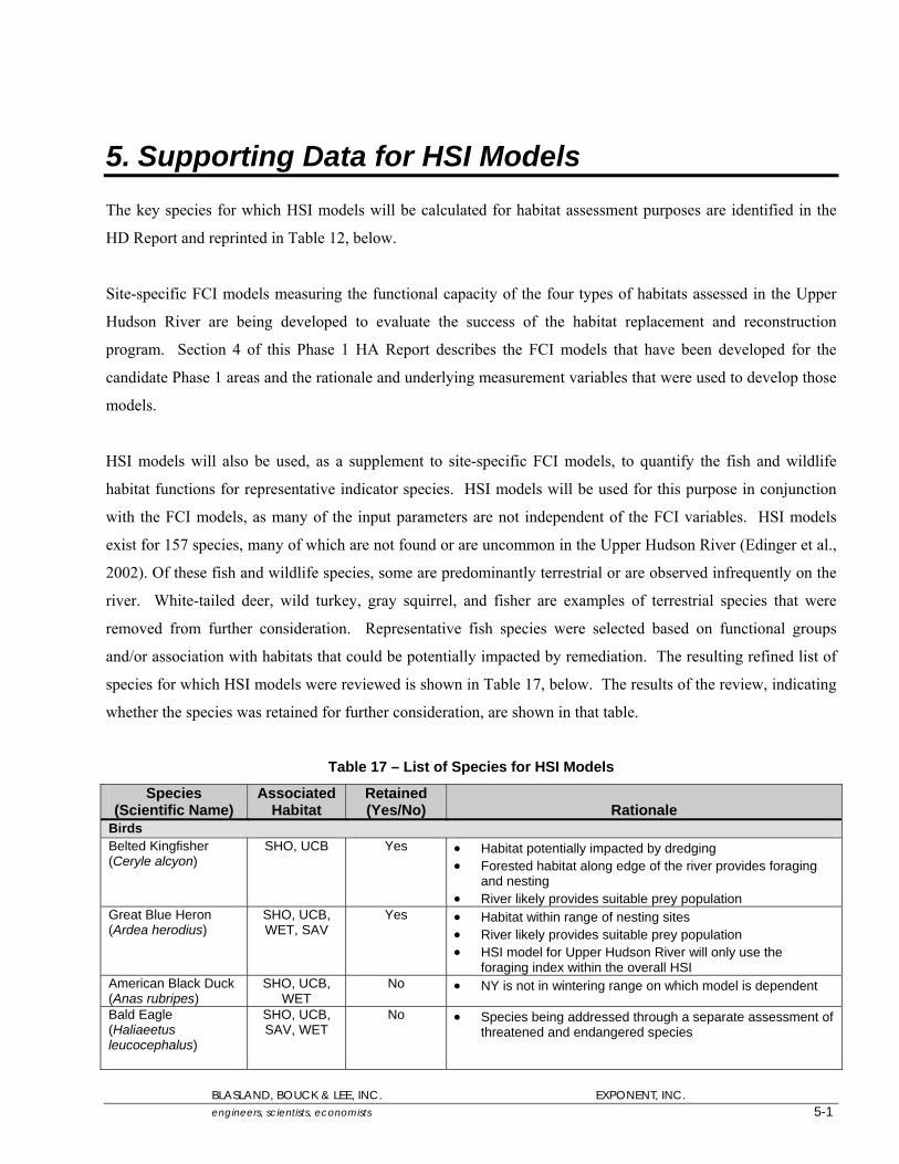
BLASLAND, BOUCK & LEE, INC. EXPONENT, INC. engineers, scientists, economists 5-1
5. Supporting Data for HSI Models The key species for which HSI models will be calculated for habitat assessment purposes are identified in the
HD Report and reprinted in Table 12, below.
Site-specific FCI models measuring the functional capacity of the four types of habitats assessed in the Upper
Hudson River are being developed to evaluate the success of the habitat replacement and reconstruction
program. Section 4 of this Phase 1 HA Report describes the FCI models that have been developed for the
candidate Phase 1 areas and the rationale and underlying measurement variables that were used to develop those
models.
HSI models will also be used, as a supplement to site-specific FCI models, to quantify the fish and wildlife
habitat functions for representative indicator species. HSI models will be used for this purpose in conjunction
with the FCI models, as many of the input parameters are not independent of the FCI variables. HSI models
exist for 157 species, many of which are not found or are uncommon in the Upper Hudson River (Edinger et al.,
2002). Of these fish and wildlife species, some are predominantly terrestrial or are observed infrequently on the
river. White-tailed deer, wild turkey, gray squirrel, and fisher are examples of terrestrial species that were
removed from further consideration. Representative fish species were selected based on functional groups
and/or association with habitats that could be potentially impacted by remediation. The resulting refined list of
species for which HSI models were reviewed is shown in Table 17, below. The results of the review, indicating
whether the species was retained for further consideration, are shown in that table.
Table 17 – List of Species for HSI Models
Species (Scientific Name)
Associated Habitat
Retained (Yes/No) Rationale
Birds Belted Kingfisher (Ceryle alcyon)
SHO, UCB Yes • Habitat potentially impacted by dredging • Forested habitat along edge of the river provides foraging
and nesting • River likely provides suitable prey population
Great Blue Heron (Ardea herodius)
SHO, UCB, WET, SAV
Yes • Habitat within range of nesting sites • River likely provides suitable prey population • HSI model for Upper Hudson River will only use the
foraging index within the overall HSI American Black Duck (Anas rubripes)
SHO, UCB, WET
No • NY is not in wintering range on which model is dependent
Bald Eagle (Haliaeetus leucocephalus)
SHO, UCB, SAV, WET
No • Species being addressed through a separate assessment of threatened and endangered species

BLASLAND, BOUCK & LEE, INC. EXPONENT, INC. engineers, scientists, economists 5-2
Species (Scientific Name)
Associated Habitat
Retained (Yes/No) Rationale
Lesser Scaup (Athya affinis)
SHO, UCB, WET
No • HSI model for wintering range applicable only to Gulf of Mexico and southern Atlantic coast
• HSI model for the breeding range applicable to the Rocky Mountain area
Great Egret (Ardea alba)
SHO, UCB, WET, SAV
No • HSI applicable only to Atlantic coast, inland Southeastern United States, Texas, and Louisiana coastal wetlands
Pileated Woodpecker (Dryocopus pileatus)
SHO No • HSI is only applicable to terrestrial and forested wetland habitats that are unlikely to be impacted remedial activities
Wood Duck (Aix sponsa)
SHO, UCB, WET, SAV
Yes • Forested wetlands along river provide potential nesting sites • Overhang and downfall along natural shorelines provide
potential cover Mammals Beaver (Castor Canadensis)
SHO, WET, SAV
No • Close proximity of roadways inconsistent with HSI requirements
Mink (Mustela vison) SHO, WET Yes • Portions of potential mink habitat in near-shore areas could be impacted by remedial activities; therefore mink has been retained as requested by the USEPA
Muskrat (Ondatra zibethicus)
SHO, WET, SAV
Yes • Abundant herbaceous vegetation on shoreline and in wetlands
• Low flow conditions of Upper Hudson River still provide surface water
• Tracks frequently observed during assessment of fringing wetlands
Fish Yellow Perch (Perca flavescens)
UCB, SAV Yes • Habitat potentially impacted by dredging • Recreational species • Predator/invertivore
Largemouth Bass (Micropterus salmoides)
UCB, WET, SAV
Yes • Habitat potentially impacted by dredging • Recreational species • Top predator
Smallmouth Bass (Micropterus dolomieui)
UCB. SAV Yes • Habitat potentially impacted by dredging • Predator/invertivore
Common Shiner (Notropis cornutus)
UCB, WET, SAV
Yes • Habitat potentially impacted by dredging • Representative HSI species for Cyprinidae • Forage base for predatory fish and fish-eating birds
Carp (Cyprinus carpio)
UCB, WET, SAV
No • Non-native and nuisance species • Species resistant to habitat modification
Bluegill (Lepomis macrochirus)
UCB, WET, SAV
Yes • Large woody debris and SAV provide cover
Channel Catfish (Ictalurus punctatus)
UCB, SAV No • Non-native species
Reptiles/Amphibians Bullfrog (Rana catesbeiana)
SHO, WET, SAV
No • HSI applicable only to Midwestern United States
Slider Turtle (Pseudemys scripta)
SHO, WET, SAV
No • HSI applicable only to Southeastern United States
Snapping Turtle (Chelydra serpentina)
SHO, UCB, WET, SAV
Yes • Small tributaries and backwaters present along river edge • Depths in river exceed ice depth; provides overwintering
BLASLAND, BOUCK & LEE, INC. EXPONENT, INC. engineers, scientists, economists 5-3
Notes: UCB = Unconsolidated river bottom SAV = Submerged aquatic vegetation SHO = Shoreline WET = Wetland
Key species for which HSI models will be calculated are the belted kingfisher, great blue heron, wood duck,
muskrat, mink, yellow perch, largemouth bass, smallmouth bass, common shiner, bluegill, and snapping turtle
(Allen, 1986; Allen and Hoffman, 1984; Edwards et al., 1983; Graves and Anderson, 1987; Krieger et al., 1983;
Prose, 1985; Short and Cooper, 1985; Sousa and Farmer, 1983; Stuber et al., 1982a, b; Trial et al., 1983). Each
of these key species is dependent on river habitat that may potentially be directly impacted by sediment removal
activities. These species have also been directly or indirectly (e.g., through signs) observed in areas where
dredging is likely to occur. The HSI models and data variables for these species are shown in Appendix I.
Where models exist for both lacustrine and riverine environments, the riverine models were used. In some cases,
such as with the great blue heron, only one index of the overall HSI will be used (the foraging index) as the
remaining variables are specific to habitats unlikely to be impacted by remedial activities (i.e., forested wetlands
off the river). A rationale for the exclusion of certain variables from the HSI models is provided in Appendix I.
Some of the data needed for the HSI models listed in Appendix I have been, or will be, collected under separate
programs, including the HDA Program, SSAP, and BMP. The necessary additional data for the HSI models
(beyond that which is, or will be, collected under established sampling programs) are described in subsection 6.4
of this Phase 1 HA Report; these data were collected in 2005.
BLASLAND, BOUCK & LEE, INC. EXPONENT, INC. engineers, scientists, economists 6-1
6. Data Needs for Phase 1 Areas The HDA Work Plan specifies that the Phase 1 HA Report will identify any additional habitat assessment data
needs. When this Phase 1 HA Report was initially prepared in April 2004, there were numerous additional
habitat assessment data needs in Phase 1 areas, and this Section 6 was included in the report to identify those
data needs and to propose additional investigations to satisfy those data needs. Since that time, most of these
investigations have been completed. As noted above, spot checking and reassessment at a limited number of
stations assessed in 2003 were conducted in 2004. Section 6.1 of this section describes that effort. The
remainder of this section identifies additional data needs to complete the habitat assessment of the Phase 1 areas.
As also noted above, most of those data collection efforts were completed in 2005 in accordance with the
SHAWP, and the results will be presented in the Phase 1 Final Design Report. While they are still included as
data needs in this report, this section identifies the data collection activities that were conducted in 2005.
6.1 Spot-Checking and Reassessment in 2004 The HDA Work Plan states that a subset of assessed areas will be spot-checked in subsequent years to assess
fluctuations in size and location of habitat types, particularly SAV beds. If substantial changes occurred in
habitat characteristics (e.g., percent cover, species composition, or size of the habitat) at a given station, the
station is to be re-sampled in accordance with the SOPs provided as Appendices A through D of this Phase 1
HA Report. Such spot checking and reassessment activities were conducted in 2004, as described below.
Due to the limited number of stations assessed in 2003, each station was visually examined to determine if
substantial changes had occurred in the size, location, percent cover, or species composition of the habitat. The
percent cover at some of the wetland stations was estimated to be less than that observed in 2003. As such, a
“substantial change” was determined to have occurred, and one riverine wetland station was randomly selected
and reassessed. In addition, water levels within River Sections 1 and 2 were elevated compared to the time at
which the 2003 assessments were completed (average flow of 2898 cfs in 2003 versus average flow of 6778 cfs
in 2004 during the same period). As such, many of the shoreline characteristics (e.g., slope) were difficult to
visually compare with the 2003 results. Although no “substantial changes” were identified, four shoreline
stations were reassessed due to the change in field conditions. Finally, as a conservative measure, stations from
each of the other habitat types were also randomly selected and reassessed. A total of 2 unconsolidated river
bottom, 1 aquatic vegetation bed, 4 shoreline, and 1 wetland station were reassessed in 2004. Data from the
reassessment are provided in Appendix K. Those data were used to calculate new FCI values for comparison

BLASLAND, BOUCK & LEE, INC. EXPONENT, INC. engineers, scientists, economists 6-2
with 2003 FCI values (see Table 18). FCI values at the stations assessed in 2003 and reassessed in 2004 varied
+/- 21%, which may indicate the level of variability that can be expected within the Upper Hudson River under
normal conditions.
Table 18 – Calculated FCI Values for Phase 1 Areas Assessed in 2003 and Reassessed in 2004
Unconsolidated River Bottom Potential to Support Macroinvertebrates
Potential to Support Fish Populations
Station FCIUNVEGBMI FCIUNVEGFISH
UCB-2 (2003) 0.88 0.77 UCB-2 (2004) 0.83 0.69 UCB-3 (2003) 0.49 0.82 UCB-3 (2004) 0.44 0.65
Aquatic Vegetation Bed Support PMI/BMI
Populations Fish and
Wildlife HabitatStabilization of
Substrate Nutrient Cycling
Station FCISAVMACROS FCISAVFISH FCISAVSTAB FCISAVNUTS
SAV-4 (2003) 0.62 0.62 0.32 0.50 SAV-4 (2004) 0.58 0.62 0.32 0.47
Shoreline Shoreline Stability Shade and Cover Wildlife Habitat Station FCISHORESTAB FCISHORECOV FCISHOREHAB
1R (2003) 0.96 0.56 0.65 1R (2004) 0.96 0.53 0.64 2I (2003) 0.83 0.46 0.59 2I (2004) 0.97 0.58 0.68 6I (2003) 1.00 0.57 0.68 6I (2004) 0.94 0.57 0.66 9I (2004) 0.99 0.57 0.67 9I (2004) 0.90 0.57 0.64
Wetland Surface-water
Exchange Energy
Dissipation
Nutrient and Organic Cycling
Maintain Character
Plant Community
Wildlife Habitat
Station FCIWATEREX FCIED FCIWETCYCLING FCIMAINTAINSPP FCIWETHAB
3 (2003) 0.76 0.61 0.64 0.65 0.60 3 (2004) 0.87 0.69 0.63 0.75 0.76
6.2 Assessments in Remaining Phase 1 Areas The HDA Work Plan specified that, in total, assessments would be completed at 136 unconsolidated river
bottom, 52 aquatic vegetation bed, 68 shoreline, and 10 riverine fringing wetland habitat stations. The number
of stations was modified to provide flexibility to evaluate variability in characteristics within aquatic vegetation
beds and fringing wetlands. Additional data on these habitats may assist in habitat reconstruction and
achievement of attaining success criteria, as described in Section 2 of the SHAWP (BBL and Exponent, 2005b).
The assessments for each habitat type follow a balanced design – i.e., 50% of the total stations are to be areas
BLASLAND, BOUCK & LEE, INC. EXPONENT, INC. engineers, scientists, economists 6-3
that may potentially be impacted by dredging (target stations), and the remaining 50% of the stations are to be in
reference locations outside of dredge areas (reference stations).
At the time the RD AOC was executed in August 2003, neither the habitat delineations nor the dredge area
delineations for the Phase 1 areas had been completed. As a result, specific habitat station locations for the
candidate Phase 1 areas were selected based on sediment type, overlying water depth, adjacent land use,
proximity to other habitat features (e.g., NYSDEC-designated wetlands), and draft working copies of the
preliminary dredge areas. This process resulted in the selection of 29 unconsolidated river bottom, 11 aquatic
vegetation bed, 16 shoreline, and three riverine fringing wetland stations in candidate Phase 1 areas. The
locations for an equal number of reference stations could not be finalized due to the status of the dredge area and
habitat delineations.
Moreover, at that time, there was not sufficient time left in the 2003 field season to complete detailed habitat
assessments at all the identified stations. As a result, only a subset of the assessment stations in candidate Phase
1 areas could be assessed in detail within the remaining sampling windows in 2003. Specifically, as described
in Section 3, habitat assessments in 2003 were completed at six unconsolidated river bottom stations, nine
aquatic vegetation bed stations, 14 shoreline stations, and four riverine fringing wetland stations. Therefore,
habitat assessments remained to be completed at the remaining stations in the Phase 1 areas (as well as in the
Phase 2 areas).
As discussed above, the SHAWP finalized in September 2005 proposed the locations of habitat assessment
stations in the remaining Phase 1 areas and in additional suitable reference areas. These additional stations
included 41 unconsolidated river bottom stations (19 target and 22 reference), seven aquatic vegetation bed
stations (all reference), six shoreline stations (all reference), and two riverine fringing wetland stations (both
target). Habitat assessments were conducted at these stations in 2005, with the results to be incorporated into
the Phase 1 Final Design Report. Subsequent habitat field work may need to be completed to evaluate inter-
annual variability and/or fill data gaps. The results of the post-2005 assessments will be incorporated in the
Phase 2 HA Report.
6.3 Data Needs for FCI Models Additional data needs were identified to complete the FCI models. These are described below. These data have
been collected in 2005 from the candidate Phase 1 areas previously sampled in 2003, the Phase 1 areas sampled

BLASLAND, BOUCK & LEE, INC. EXPONENT, INC. engineers, scientists, economists 6-4
in 2005, and some Phase 2 areas, and will continue to be collected from Phase 2 areas to be assessed in the
future.
6.3.1 Current Velocity Current velocities were recorded in 2003 at 10 cm and 1 m above the substrate within unconsolidated river
bottom and aquatic vegetation bed habitats. Because velocity typically increases exponentially from the bottom
to just near the surface, recordings taken from set depths above the substrate may not be comparable among
stations. Therefore, current velocity data collected in 2005 included not only the measurements at 10 cm and 1
m above the substrate, but also measurements at 80% and 20% of the water depth so that these data can be
normalized to water depth to allow between station comparisons. In addition, current velocity was measured at
60% of the water depth for use in the HSI models. These measurements will continue to be made in the future.
Current velocity measurements are being collected as part of the BMP and Supplemental Engineering Data
Collection (SEDC) Program at multiple transect locations under low (less than 3,000 cfs), moderate (3,000 to
7,000 cfs), and high (greater than 7,000 cfs) flows. These data will be used to update the QEA 2-D
hydrodynamic model (QEA 1999a, b), which may be used to predict areas of higher or lower current. Current
velocity measurements collected in the candidate Phase 1 areas sampled in 2003 and during the habitat
assessments of the remaining Phase 1 areas and the Phase 2 areas will be compared with the BMP and SEDC
measurements to determine maximum flow conditions in the unconsolidated river bottom and aquatic vegetation
beds (based on measurements collected inside the beds). In addition, current velocity measurements taken at
unconsolidated river bottom and aquatic vegetation beds (inside and outside of bed) will be used in the HSI
models for several fish species.
6.3.2 Inundation Period During the assessments for riverine fringing wetlands, it was determined that these habitats lack true O and A
horizons. The three preliminary functions (listed in Table 2 of the HDA Work Plan) that depend on these soil
property variables (“export organic carbon,” “nutrient cycling,” and “remove and hold elements and
compounds”) were combined to provide one function (“nutrient and organic cycling”) related to the ability of
the wetland to import and/or export nutrients and organic carbon. Fundamental to the nutrient and organic
cycling function is contact of the river water with the wetland – currently being quantified by the surface-water
exchange function. The function will be revised to include inundation period to more accurately reflect the

BLASLAND, BOUCK & LEE, INC. EXPONENT, INC. engineers, scientists, economists 6-5
surface-water exchange (Shafer and Yozzo, 1998). Data on inundation period during the growing season have
been collected in 2005 in the Phase 1 areas sampled in 2003, the remaining Phase 1 areas, and some Phase 2
areas, and will continue to be collected from Phase 2 areas to be sampled in the future. In the Upper Hudson
River, fluctuations due to the hydrofacilities typically occur on a daily cycle with resulting changes in water
depth and flow of up to 18 inches (6 to 12 inches typically) and 5,000 cfs respectively for a duration of 6 to 12
hours. Due to the water level fluctuations, the mean daily water elevations during the growing season will be
used for water depth. In addition, minimum and maximum daily water elevations during the growing season
will be reported in the Phase 1 Final Design Report. The inundation period will be evaluated as number of days
inundated during the growing season. The start and end of the growing season will be obtained from Natural
Resource Conservation Service soil surveys. Elevations used in habitat reconstruction design will be derived
from ecological benchmarks present in reference riverine fringing wetlands/aquatic vegetation beds. To
supplement ecological benchmark information, water level measurements obtained during riverine fringing
wetland assessments will be correlated with available river gauge measurements.
6.3.3 Validation of FCI Models Additional site-specific data may be necessary to support the full development of the FCI model equations. The
FCI models presented in this Phase 1 HA Report are primarily based on the literature and professional judgment.
Site-specific data may be used to calibrate, verify, and/or validate the FCI models for the Upper Hudson River.
Some such site-specific data are currently being collected, or are planned to be collected, under the HDA
program or other programs. These data sources include the following:
• Existing Data. Relevant existing data from former studies (e.g., Law Environmental, 1991, and Exponent,
1998) will be used with the additional field data to revise the FCI models. In addition, GE’s catch-per-unit-
effort data from its fish sampling activities, as well as other existing resource agency data (to the extent they
are made available to GE), will be used to further develop the FCI models.
• Functional Data Assessment. To the extent available, direct functional data relating to the secondary success
criteria, such as fish and wildlife observations being collected under other programs (e.g., the Baseline
Monitoring Program) and the current habitat assessment program, will be used to calibrate the fish and
wildlife support functions. To enhance the ability to use such data, habitat assessment activities at the
remaining stations (all of which currently represent reference conditions) will include more quantitative fish
and wildlife observations that include a temporal component at dawn and dusk. The life stage of organisms
BLASLAND, BOUCK & LEE, INC. EXPONENT, INC. engineers, scientists, economists 6-6
observed, to the degree that life stage can be determined during observational activities, will be recorded.
These observations and recordings were made during the habitat assessment activities conducted in 2005. In
addition, if, after dredging, functional data such as invertebrate, fish and wildlife observations beyond those
being collected under the other programs mentioned above (e.g., benthic invertebrate community analysis)
would be useful to judge success under the secondary success criteria, appropriate studies and data collection
may be implemented at that time in both dredged areas and non-impacted reference areas. If such data are
adequate to support reliable evaluations, they will provide an additional line of evidence for calibrating the
precision and accuracy of the FCI models insofar as they relate to fish and wildlife support functions.
• Ongoing Data Collection. Data from other on-going sampling programs can also be used to verify or validate
FCI models. For example, data obtained from the SEDC program, under which information on physical
features of the Upper Hudson River is being collected to aid in the final design process, can be used to verify
values of certain FCI variables. Similarly, fish and/or macroinvertebrate data currently collected by the
resource agencies (to the extent such data are made available to GE) or others may be used to aid in validating
FCI models if data quality objectives of the HDA program are satisfied.
6.4 Data Needs for HSI Models Post-dredging comparisons of habitat parameters in the target areas to those in the reference area data set will
provide the primary basis for determining the success of the habitat replacement and reconstruction program
(Section 4.6 and BBL, 2003b). As stated in the HDA Work Plan, the FCI models are being used to relate
habitat-specific parameters to the functions provided by those habitats. Similarly, as noted above, HSI models
will also be used in conjunction with site-specific FCI models for fish and wildlife habitat function for
representative indicator species.
As discussed in the HD Report and in Section 5 of this Phase 1 HA Report, HSI models will be developed for
the following species:
• Belted Kingfisher (Ceryle alcyon);
• Great Blue Heron (Ardea herodius);
• Wood Duck (Aix sponsa);
• Muskrat (Ondatra zibethicus);
• Mink (Mustela vison);

BLASLAND, BOUCK & LEE, INC. EXPONENT, INC. engineers, scientists, economists 6-7
• Snapping Turtle (Chelydra serpentina);
• Yellow Perch (Perca flavescens);
• Largemouth Bass (Micropterus salmoides);
• Smallmouth Bass (Micropterus dolomieui);
• Bluegill (Lepomis macrochirus); and
• Common Shiner (Notropis cornutus).
For these HSI models, there are several model variables where additional data are needed. As one example, for
the largemouth bass HSI model, data on average water temperature within pools, backwaters, or littoral areas
during the growing season, minimum DO levels during midsummer within pools or littoral areas, and pH range
during the growing season may be needed. These data are not currently collected under existing sampling and
analyses programs (e.g., HDA, SSAP, or BMP).
Appendix I provides the complete list of variables proposed for collection for each of the above-listed species.
The SHAWP submitted in September 2005 specified the number of stations and locations for the collection of
additional data to support these HSI models, as well as the specific data proposed for collection. These data
were collected in 2005.
6.5 Assessments in Off-Site Reference Areas As discussed in the HD Report, reference stations for each of the four habitats (i.e., unconsolidated river bottom,
aquatic vegetation bed, shoreline, and fringing wetland) will be selected for detailed assessment in appropriate
locations of the Upstream Upper Hudson and/or Lower Mohawk River. The specific locations for conducting
detailed habitat assessments in these off-site reference areas are tentatively identified in the SHAWP, subject to
change based on field conditions. Further data collection in off-site reference areas is currently scheduled for
2006. Habitat assessment procedures will follow methods described in the SOPs provided as Appendices A
through D of this Phase 1 HA Report.
6.6 Spot-Checking and Reassessment in Subsequent Seasons As noted in subsection 6.1 above, the HDA Work Plan states that a subset of assessed areas will be spot-checked
in subsequent years to assess fluctuations in size and location of habitat types, particularly aquatic vegetation
beds, and that if substantial changes occurred in habitat characteristics at a given station, the station is to be re-

BLASLAND, BOUCK & LEE, INC. EXPONENT, INC. engineers, scientists, economists 6-8
sampled in accordance with the SOPs provided as Appendices A through D of this Phase 1 HA Report and the
HDA Work Plan. The spot-checking and reassessment approach described in the HDA Work Plan and
implemented for the stations that were spot-checked in 2004 (see subsection 6.1) relies on a “visual
examination” for deciding which stations would need to be reassessed. For subsequent field seasons before
dredging begins, GE proposes to follow a revised spot-checking/reassessment approach that will remove the
potential source of uncertainty (i.e., the visual examination step) from the process. Specifically, in those field
seasons, a minimum of one station and maximum of two stations for unconsolidated river bottom, aquatic
vegetation bed and shoreline habitats will be reassessed within each river reach (as defined in the BMP QAPP
[QEA 2003]), for a total number of reassessment stations not to exceed 24 stations. For the riverine fringing
wetlands, one station will be reassessed within each river reach, for a total number of wetland reassessment
stations not to exceed four stations. The specific station(s) to be reassessed will be randomly selected from the
stations assessed in the previous season, including those stations identified as visibly different from previous
years. If the preliminary results from the initial reassassements indicate that any habitat-specific parameters have
changed considerably, additional stations may be reassessed. The reassessment results will be provided in the
Final Design Report for Phase 2 or other appropriate report to USEPA relating to the HDA or adaptive
management program.
In addition, in each subsequent field season, all stations to be assessed or reassessed will first be groundtruthed
to verify the originally delineated boundaries of that habitat. For the aquatic vegetation bed and unconsolidated
river bottom habitats, stratified (depth-based) random groundtruthing will be used to determine whether the
delineated area has changed.
6.7 Schedule As discussed above, most of the investigations described above in this section to satisfy the identified data needs
in Phase 1 areas were conducted in 2004 or 2005. The investigations described in subsection 6.5 will be
conducted in the 2006 field season, and those described in subsection 6.6 will be conducted in that and
subsequent field seasons.
BLASLAND, BOUCK & LEE, INC. EXPONENT, INC. engineers, scientists, economists 7-1
7. References Allen, A.W. 1986. Habitat suitability index models: Mink, revised. U.S. Dept. Int., USFWS. Biol. Rep.
82(10.127). 23 pp.
Allen, A.W. and R. D. Hoffman. 1984. Habitat suitability index models: Muskrat. U.S. Dept. Int., USFWS.
FWS/OBS-82/10.46. 27 pp.
Ainslie, W.B., R.D. Smith, B.A. Pruitt, T.H. Roberts, E.J. Sparks, L. West, G.L. Godshalk, and M.V. Miller.
1999. A Regional Guidebook for Assessing the Functions of Low Gradient, River Wetlands in Western Kentucky.
Technical Report WRP-DE-17, US Army Engineer Waterways Experiment Station, Vicksburg, MS.
Angradi, T.R. 1999. Fine sediment and macroinvertebrate assemblages in Appalachian streams: A field
experiment with biomonitoring applications. J. N. Am. Benthol. Soc. 18(1):49− 66.
Bain, M.B. and S.E. Boltz. 1992. Effect of aquatic plant control on the microdistribution and population
characteristics of largemouth bass. Trans. Amer. Fish. Soc. 121:94–103.
Barbour, M.T., J. Gerritsen, B.D. Snyder, and J.B. Stribling. 1999. Rapid Bioassessment Protocols for Use in
Streams and Wadeable Rivers: Periphyton, Benthic Macroinvertebrates, and Fish, Second Edition. EPA 841-B-
99-002. USEPA, Office of Water, Washington, DC.
BBL. 2003a. Remedial Design Work Plan (RD Work Plan). Hudson River PCBs Superfund Site. Prepared for
General Electric Company, Albany, NY.
BBL. 2003b. Habitat Delineation and Assessment Work Plan (HDA Work Plan). Hudson River PCBs
Superfund Site. Prepared for General Electric Company, Albany, NY.
BBL and Exponent. 2005a. Habitat Delineation Report (HD Report). Hudson River PCBs Superfund Site.
Prepared for General Electric Company, Albany, NY.
BBL and Exponent. 2005b. Supplemental Habitat Assessment Work Plan (SHAWP). Hudson River PCBs
Superfund Site. Prepared for General Electric Company, Albany, NY.
BLASLAND, BOUCK & LEE, INC. EXPONENT, INC. engineers, scientists, economists 7-2
Brazner, J.C. and J.J. Magnuson. 1994. Patterns of fish species richness and abundance in coastal marshes and
other nearshore habitats in Green Bay, Lake Michigan. Verh. Internat. Verein. Limnol. 25:2098–2104.
Brinson, M.M., F.R. Hauer, L.C. Lee, W.L. Nutter, R.D. Rheinhardt, R.D. Smith, and D. Whigham. 1995. A
Guidebook for Application of Hydrogeomorphic Assessments to Riverine Wetlands. Technical Report WRPDE-
11. U.S. Army Engineer Waterways Experiment Station. Vicksburg, MS.
Caraco, N.F. and J.J. Cole. 2002 Contrasting impacts of a native and alien macrophytes on dissolved oxygen in a
large river. Ecol. Appl. 12(5):1496-1509.
Carpenter, S.R. and D.M. Lodge. 1986. Effects on submersed macrophytes on ecosystem processes. Aquat. Bot.
26: 341-370.
Casselman, J.M. and C.A. Lewis. 1996. Habitat requirements of northern pike (Esox lucius). Can. J. Fish.
Aquat. Sci. 53 (Suppl. 1): 161-174.Clairain, E.J. Jr. 2002. Hydrogeomorphic Approach to Assessing Wetland
Functions: Guidelines for Developing Regional Guidebook; Chapter 1, Introduction and Overview of the
Hydrogeomorphic Approach. ERDC/EL TR-02-3. U.S. Army Engineer Research and Development Center,
Vicksburg, MS.
Clairain, E.J. Jr. 2002. Hydrogeomorphic Approach to Assessing Wetland Functions: Guidelines for Developing
Regional Guidebook; Chapter 1, Introduction and Overview of the Hydrogeomorphic Approach. ERDC/EL TR-
02-3. U.S. Army Engineer Research and Development Center, Vicksburg, MS.
Cyr, H. and J.A. Downing. 1998. The abundance of phytophilous invertebrates on different species of
submerged macrophytes. Freshwater Biol. 20(3):365–374.
Danehy, R.J., N.H. Ringler, and J.E. Gannon. 1991. Influence of nearshore structure on growth and diets of
yellow perch (Perca flavescens) and white perch (Morone americana) in Mexico Bay, Lake Ontario. J. Great
Lakes Res., 17:183–193.
Diehl, S. 1993. Effects of habitat structure on resource availability, diet and growth of benthivorous perch,
Perca fluviatilis. Oikos 67:403− 414.
BLASLAND, BOUCK & LEE, INC. EXPONENT, INC. engineers, scientists, economists 7-3
Diehl, S. and R. Kornijow. 1998. Influence of submerged macrophytes on trophic interactions among fish and
macroinvertebrates. Pages 24-46 In Jeppesen, E., M. et al. (eds). The Structuring Role of Submerged
Macrophytes in Lakes (Ecological Studies 131). Springer Verlag, New York.
Downing, J.A. and M.R. Anderson. 1985. Estimating the Standing Biomass of Aquatic Macrophytes. Can. J.
Fish. Aquat. Sci. 42:1860-1869.
Ecology and Environment. 2003. Hudson River Superfund Site, Facility Siting Data Summary Report, Site-
Specific Field Investigations of the Final Sites. December 2003.
Edinger, G.J., D.J. Evans, S. Gebauer, T.G. Howard, D.M. Hunt, and A.M. Olivero (eds.). 2002. Ecological
Communities of New York State. Second Edition. A revised and expanded edition of Carol Reschke's
Ecological Communities of New York State. (Draft for review). New York Natural Heritage Program, NYSDEC,
Albany, NY.
Edwards, E. A., G. Gebhart, and O.E. Maughan. 1983. Habitat suitability information: Smallmouth bass. U.S.
Dept. Int., USFWS. FWS/OBS-82/10.36. 47 pp.
Exponent. 1998. Data Documentation and Interpretation Report: SAV and Fish Community Analysis. Prepared
for the General Electric Company, Albany, NY.
Findlay, S.E. G., E. Kiviat, W.C. Nieder, and E.A. Blair. 2002. Functional assessment of a reference wetland set
as a tool for science, management and restoration. Aquat. Sci. 64:107-117.
Findlay, S.E. W.C. Nieder, and D.T. Fishcer. In Review. Multi-scale controls on water quality effects of
submerged aquatic vegetation in the tidal freshwater Hudson River. Ecosystems.
Fonseca, M.S., B.E. Julius, and W.J. Kenworthy. 2000. Integrating biology and economics in seagrass
restoration: How much is enough and why? Eco. Eng. 15:227-237.
Gerrish, N. and J.M. Bristow. 1979. Macroinvertebrate associations with aquatic macrophytes and artificial
substrates. J. Great Lakes Res. 5(1):69–72.
BLASLAND, BOUCK & LEE, INC. EXPONENT, INC. engineers, scientists, economists 7-4
Gotceitas, V. and P. Colgan. 1987. Selection between densities of artificial vegetation by young bluegills
avoiding predation. Trans. Amer. Fish. Soc. 116:40–49.
Graves, B.M., and S.H. Anderson. 1987. Habitat suitability index models: Snapping turtle. U.S. Dept. Int.,
USFWS. Biol. Rep. 82(10.141). 18 pp.
Hayse, J.W. and T.E. Wissing. 1996. Effects of stem density of artificial vegetation on abundance and growth of
age-0 bluegills and predation by largemouth bass. Trans. Amer. Fish. Soc., 125:422–433.
Helfman, G. S. 1979. Twilight activities of yellow perch, Perca flavescens. J. Fish. Res. Board Can. 36(2): 173-
179.
Herman, E., W.J. Wisky, L. Wiegert, and M. Burdick. 1964. The yellow perch, its life history, ecology, and
management. Wisconsin Conserv. Dept. Publ. 228:1-14.
Hunter, C.J. 1991. Better Trout Habitat: A Guide to Stream Restoration and Management. Island Press,
Washington, DC.
Hynes, H.B.N. 1966. The Biology of Polluted Running Waters. University of Liverpool Press.
Jenkins, R.M., E.M. Leonard, and G.E. Hall. 1952. An investigation of the fisheries resource of the Illinois River
and pre-impoundment study of Tenkiller Reservoir, Oklahoma. Oklahoma Fish. Res. Lab. Rep. 26. 136 pp.
Kitchell, J. F., M.G. Johnson, C.K. Minns, K.H. Loftus, L. Greig, and C.M. Oliver. 1977. Percid habitat: The
river analogy. J. Fish. Res. Board Can. 34(10):1936-1940.
Koch, E.W. 2001. Beyond light: physical, geological and geochemical parameters as possible submersed aquatic
vegetation habitat requirements. Estuaries. 24: 1-17
Koetsier, P. and J.V. McArthur. 2000. Organic matter retention by macrophyte beds in two southeastern USA,
low-gradient, headwater streams. Journal of North American Benthological Society. 19:633-647.

BLASLAND, BOUCK & LEE, INC. EXPONENT, INC. engineers, scientists, economists 7-5
Krieger, D.A., J.W. Terrell, and P.C. Nelson. 1983. Habitat suitability information: Yellow perch. U.S. Dept.
Int., USFWS. FWS/OBS-83/10.55. 37 pp.
Law Environmental. 1991. Upper Hudson River Submerged and Emergent Aquatic Vegetation Survey. Prepared
for the General Electric Company, Albany, NY.
Madsen, J. D., P.A. Chambers, W.F. James, E.W. Koch, and D.F. Westlake. 2001. The interaction between
water movement, sediment dynamics and submersed macrophytes. Hydrobiologia. 444:71-84.
McCreary Waters, N.M. and C.R. San Giovanni. 2002. Distribution and diversity of benthic macroinvertebrates
associated with aquatic macrophytes. J. Freshwat. Biol. 17.
Mellors, J.E. 1991. An evaluation of a rapid visual technique for estimating seagrass biomass. Aquat. Bot.
42:67-73.
Merritt, R.W. and K.W. Cummins (eds.). 1984. An Introduction to the Aquatic Insects of North America.
Kendall/Hunt Publ. Co. Dubuque, IA 722 pp.
Miller, R.J. 1975. Comparative behavior of centrachid basses. Pages 85-94 in H. Clepper, ed. Black bass biology
and management. Sport Fish. Inst., Washington, DC.
Mittelbach, G.G. and C.W. Osenberg. 1993. Stage-structured interactions in bluegill: consequences of adult
resource variation. Ecology. 74(8):2381–2394.
Niedowski, N.L. 2000. New York State Salt Marsh Restoration and Monitoring Guidelines. Prepared for NYS
Department of State and NYSDEC, Albany, NY.
Prose, B. L. 1985. Habitat suitability index models: Belted kingfisher. U.S. Dept. Int., USFWS. Biol. Rep.
82(10.87). 22 pp.
QEA. 2005. Phase 1 Dredge Area Delineation Report (Phase 1 DAD Report). Hudson River PCBs Superfund
Site. Prepared for the General Electric Company. February.

BLASLAND, BOUCK & LEE, INC. EXPONENT, INC. engineers, scientists, economists 7-6
QEA. 2004. Phase 1 Target Area Identification Report (Phase 1 TAI Report). Hudson River PCBs Superfund
Site. Prepared for the General Electric Company. September.
QEA. 2003. Baseline Monitoring Program Quality Assurance Project Plan. Hudson River PCBs Site. Prepared
for General Electric Company, Albany, NY.
QEA. 1999a. PCBs in the Upper Hudson River - Volume I, Historical Perspective and Model Overview.
Prepared for General Electric Company, Albany, NY.
QEA. 1999b. PCBs in the Upper Hudson River - Volume II, A Model of PCB Fate Transport and
Bioaccumulation. Prepared for General Electric Company, Albany, NY.
Randall, R.G., J.R.M. Kelso, and C.K Minns. 1996. The relationship between an index of fish production and
submerged macrophytes and other habitat features at three littoral areas in the Great Lakes. Can. J. Fish. Aquat.
Sci.. 53 (Suppl.1):35-44.
Rosgen, D. 1996. Applied River Morphology. Wildland Hydrology, Pagosa Springs, CO.
Rozas, L.P. and W.E. Odum. 1987. The role of submerged aquatic vegetation in influencing the abundance of
nekton on contiguous tidal fresh-water marshes. J. Exp. Mar. Biol. Ecol., 114:289–300.
Schutten, J. and A.J. Davy. 2000. Predicting the hydraulic forces on submerged macrophytes from current
velocity, biomass and morphology. Oecologia. 123:445-452
Scott, A. 1987. Prey selection by juvenile cyprinids from running water. Freshwater Biology. 17:129–142.
Shafer, D.J. and D. J. Yozzo. 1998. National Guidebook for Application of Hydrogeomorphic Approach to
Assessment to Tidal Fringe. Technical Report WRP-DE-16, U.S. Army Engineer Research and Development
Center, Vicksburg, MS.
Short, H. L., and R.J. Cooper. 1985. Habitat suitability index models: Great blue heron. U.S. Dept. Int., USFWS.
Biol. Rep. 82(10.99). 23 pp.
BLASLAND, BOUCK & LEE, INC. EXPONENT, INC. engineers, scientists, economists 7-7
Smith, R.D. and J.S. Wakeley. 2001. Hydrogeomorphic approach to assessing wetland functions: Guidelines for
developing regional guidebooks. Chapter 4 - Developing assessment models. ERDC/EL TR-01-30. U.S. Army
Engineer Research and Development Center, Vicksburg, MS.
Snyder, F.L., D.O. Kelch, and J.M. Reuter. 1996. Usefulness of artificial rock structure in fish habitat
improvement. In: 39th Conference of the International Association for Great Lakes Research, Mississauga, ON.
Sousa, P. J., and A. H. Farmer. 1983. Habitat suitability index models: Wood duck. U.S. Dept. Int., USFWS.
FWS/OBS-82/10.43. 27 pp.
Sowa, S.P. and C.F. Rabeni. 1995. Regional evaluation of the relation of habitat to distribution and abundanceof
smallmouth bass and largemouth bass in Missouri streams. Trans. Amer. Fish. Soc. 124:240–251.
Stromberg, J.C., J. Fry, and D.T. Patten. 1997. Marsh development after large floods in an alluvial, arid-land
river. Wetlands. 17: 292-300.
Stuber, R. J., G. Gebhart, and O. E. Maughan. 1982a. Habitat suitability index models: Bluegill. U.S. Dept. Int.,
USFWS. FWS/OBS-82/10.8. 26 pp.
Stuber, R. J., G. Gebhart, and O. E. Maughan. 1982b. Habitat suitability index models: Largemouth bass. U.S.
Dept. Int., USFWS. FWS/OBS-82/10.16. 32 pp.
Thayer, G. W., T. A. McTigue, R. J. Bellmer, F. M. Burrows, D. H. Merkey, A. D. Nickens, S. J. Lozano, P. F.
Gayaldo, P. J. Polmateer, and P. T. Pinit. 2003. Science- Based Restoration Monitoring of Coastal Habitats,
Volume One: A Framework for Monitoring Plans Under the Estuaries and Clean Waters Act of 2000 (Public
Law 160-457). NOAA Coastal Ocean Program Decision Analysis Series No. 23, Volume 1. NOAA National
Centers for Coastal Ocean Science, Silver Spring, MD. 35 pp. plus appendices.
Trial, J. G., C. S. Wade, J. G. Stanley, and P. C. Nelson. 1983. Habitat suitability information: Common shiner.
U.S. Dept. Int., USFWS. FWS/OBS-82/10.40. 22 pp.
USEPA. 2002. Hudson River PCBs Site – Record of Decision and Responsiveness Summary (ROD). New York,
NY.
BLASLAND, BOUCK & LEE, INC. EXPONENT, INC. engineers, scientists, economists 7-8
USEPA/GE. 2003. Administrative Order on Consent for Hudson River Remedial Design and Cost Recovery
(RD AOC) (Index No. CERCLA-02-2003-2027). Effective Date August 18, 2003.
Ward, J.F. and G.G.C. Robinson. 1974. A review of research on the limnology of West Blue Lake, Manitoba. J.
Fish. Res. Board Can. 31:977-1005.
Weatherhead, M.A. and M.R. James. 2001. Distribution of macroinvertebrates in relation to physical and
biological variables in the littoral zone of nine New Zealand lakes. Hydrobiologia. 462 (1-3): 115-129.
Zalewski, M., B. Bis, M. Lapińska, P. Frankiewicz, and W. Puchalski. 1998. The importance of the riparian
ecotone and river hydraulics for sustainable basin-scale restoration scenarios. Aquat. Conserv. 8:287− 307.