habitat conservation plan for state trust lands: 2012 ... · ultimately, implementation monitoring...
TRANSCRIPT

N
A
T
U
R
A
L
R
E
S
O
U
R
C
E
S
Habitat Conservation Plan for State Trust Lands:
2012 Implementation
Monitoring
Report
March 2013
Washington State
Department of
Natural Resources:
Forest Resources Division

ii
Acknowledgements
Authors
Mike Buffo Casey Hanell Contributors
Richard Bigley Angus Brodie César Carrión Florian Deisenhofer Karen Jennings Candace Johnson Bruce Livingston Fred Martin Bob Redling Denise Roush-Livingston Julie Sackett Zak Thomas Tyler Traweek Brian Williams Photo Credit
Cover photo: Richard Bigley

iii
Table of Contents
Page List of Acronyms v
List of Figures vi
List of Tables vii
Executive Summary viii
Introduction 1
Riparian Restoration Implementation Monitoring 3
Background Information 3
Riparian Forest Restoration Monitoring 4
Methods 5
Results 7
Discussion 15
Potentially Unstable Hillslope Management Implementation Monitoring 19
Background Information 19
Methods 20
Results 21
Appendix 1 24
Appendix 2 33
References 34

iv
v
List of Acronyms
CI confidence interval
DBH diameter at breast height (4.5 feet)
DNR Washington State Department of Natural Resources
GIS Geographic Information System
GPS Global Positioning System
HCP 1997 Habitat Conservation Plan for state trust lands
LWD Large woody debris
OESF Olympic Experimental State Forest
QMD quadratic mean diameter
RD Curtis’ relative density
RDFC Riparian Desired Future Conditions
RFRS Riparian Forest Restoration Strategy
RMZ Riparian Management Zone
TPA trees per acre
WAC Washington Administrative Code
vi
List of Figures
Page Figure 1. State Trust Lands HCP planning units where the Riparian Forest Restoration Strategy applies.
3
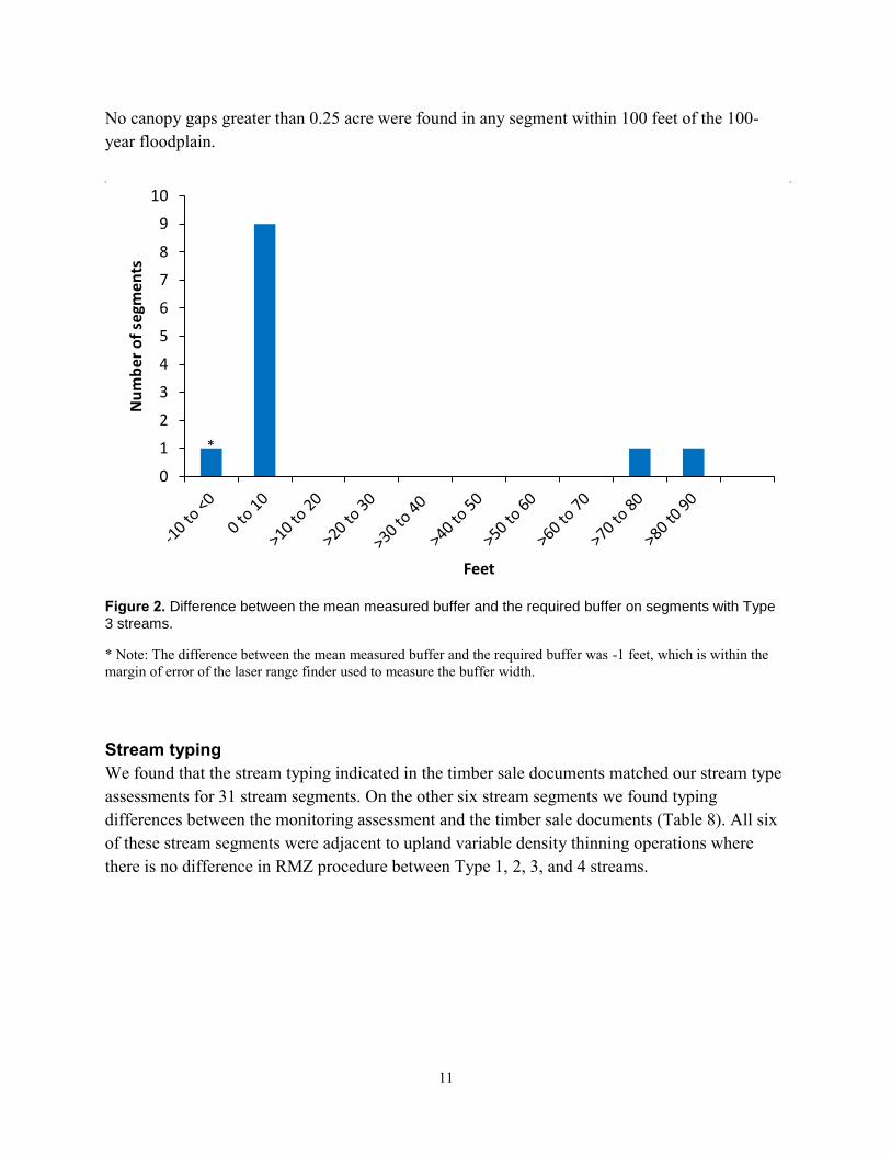
Figure 2. Difference between the mean measured buffer and the required buffer on segments with Type 3 streams.
11
Figure 3. Distribution on quadratic mean diameters by segment of large woody debris (blue; 25 segments) and snags (red; 14 segments).
13
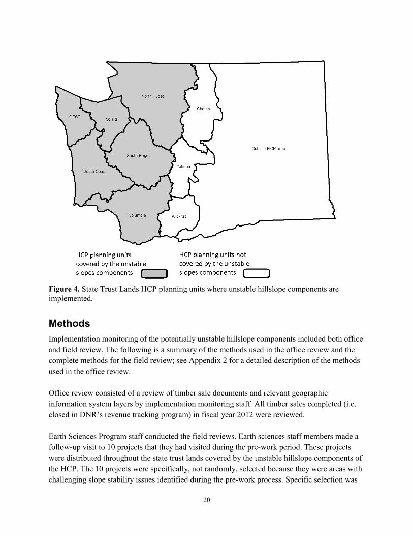
Figure 4. State Trust Lands HCP planning units where unstable hillslope components are implemented.
20
Figure A-1. Diagram of a stream system show the segment breaks between Type 3 and 4 streams. Type 5 streams were ignored in the segment selection process but are shown here for detail.
25
Figure A-2. Example of how the length of the riparian restoration area was found. Stream A has restoration activities only on one side for a length of 1000 feet. Stream B has restoration on one side for 1000 feet and on the other side for 500 feet for a total length of 1500 feet.
28
Figure A-3. Schematic of locations of plots along stream segments. 29
vii
List of Tables
Page Table 1. Riparian Desired Future Conditions (RDFC) threshold targets (Washington State Department of Natural Resources 2006a).
4
Table 2. Riparian Forest Restoration Strategy minimum parameters for prescriptions (Reproduced from Washington State Department of Natural Resources 2006a).
7
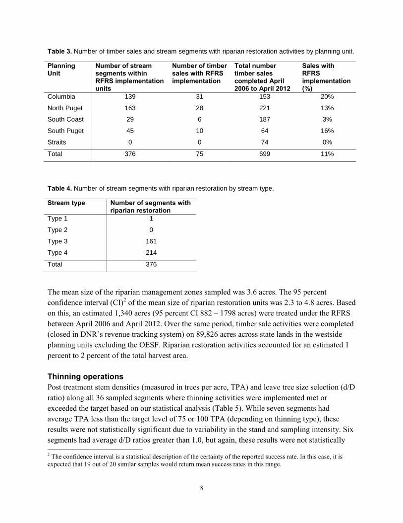
Table 3. Number of timber sales and stream segments with riparian restoration activities by planning unit.
8
Table 4. Number of stream segments with riparian restoration by stream type. 8
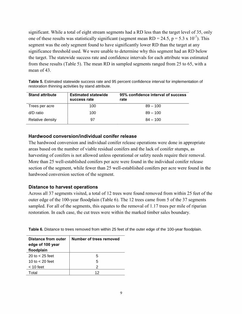
Table 5. Estimated statewide success rate and 95% confidence interval for implementation of restoration thinning activities by stand attribute.
9
Table 6. Distance to trees removed from within 25 feet of the outer edge of the 100-year floodplain.
9
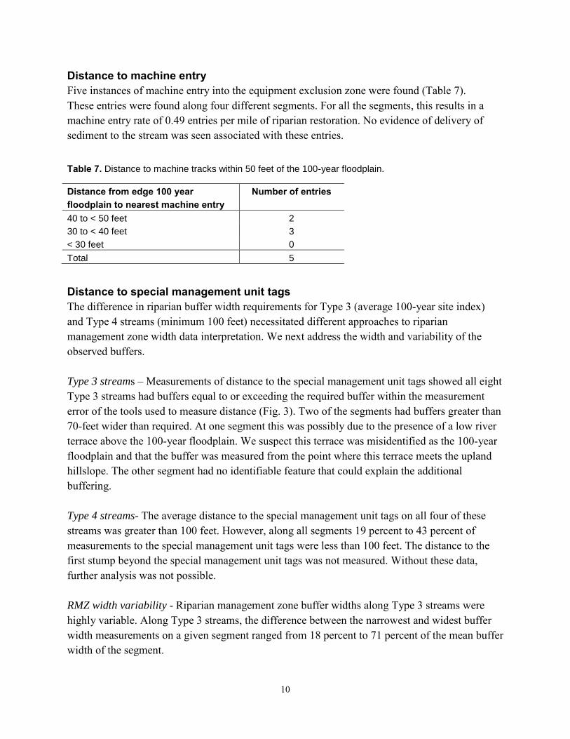
Table 7. Distance to machine tracks within 50 feet of the 100-year floodplain. 10
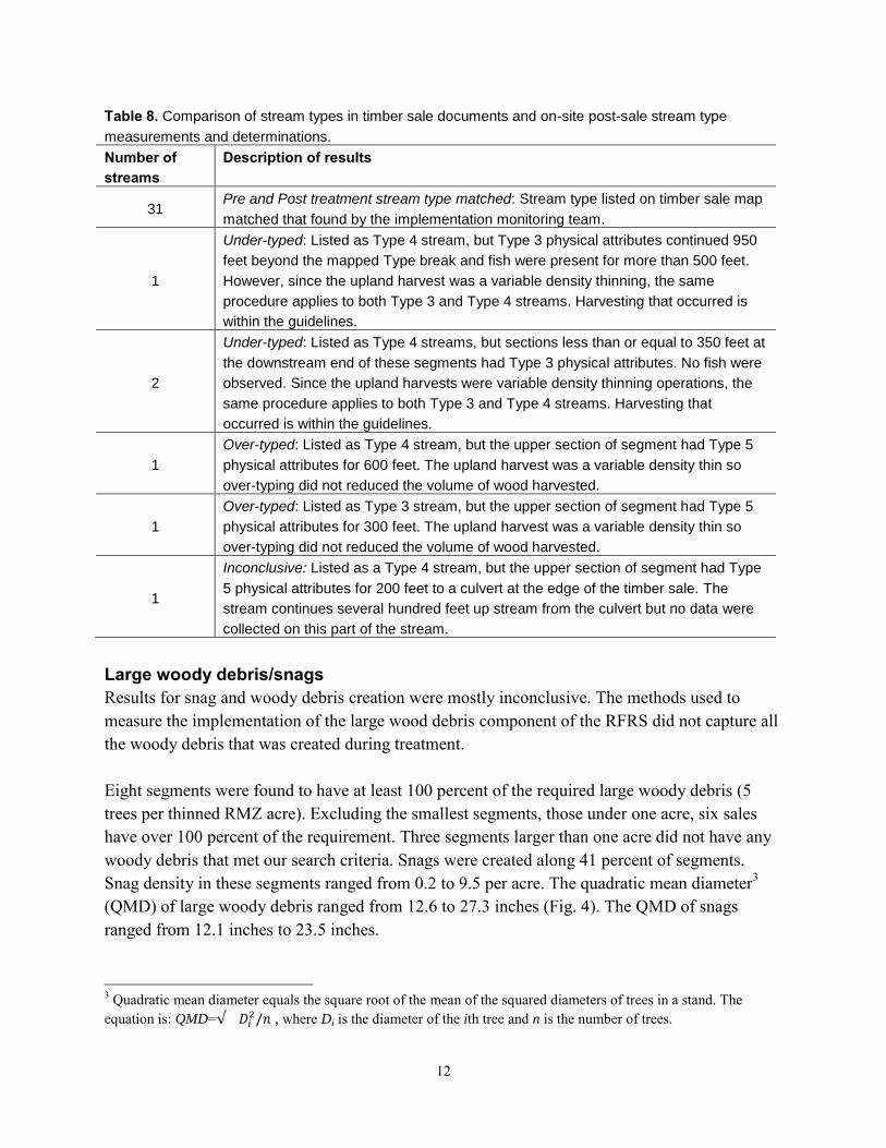
Table 8. Comparison of stream types in timber sale documents and on-site post-sale stream type measurements and determinations.
12
Table 9. Number of trees per acre and proportion of trees per acre by species pre and post-thinning in the Columbia Planning Unit.
14
Table 10. Number of trees per acre and proportion of trees per acre by species pre and post-thinning in the North Puget Planning Unit.
14
Table 11. Number of trees per acre and proportion of trees per acre by species pre and post-thinning in the South Coast Planning Unit.
14
Table 12. Number of trees per acre and proportion of trees per acre by species pre and post-thinning in the South Puget Planning Unit.
15
Table 13. Distribution of projects reviewed by completion year and type. 21
Table 14. Number timber sale polygons that intersected slope stability screening layers. 22
Table A-1. Spacing of plots along stream segments by length of segment 27
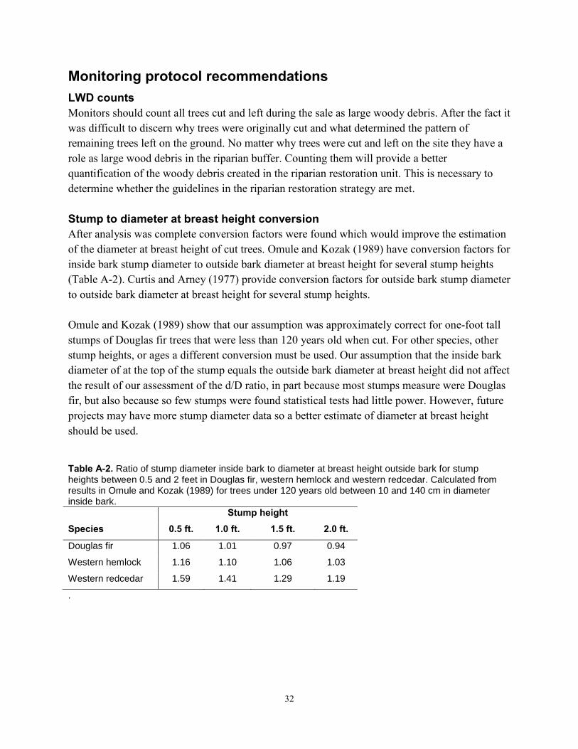
Table A-2. Ratio of stump diameter inside bark to diameter at breast height outside bark for stump heights between 0.5 and 2 feet in Douglas fir, western hemlock and western redcedar. Calculated from results in Omule and Kozak (1989) for trees under 120 years old between 10 and 140 cm in diameter inside bark.
32
viii
Executive Summary
State Trust Lands Habitat Conservation Plan (HCP) implementation monitoring informs managers on how well the habitat conservation strategies described in the State Trust Lands HCP are being applied across the landscape. Implementation monitoring is a critical first step in laying the foundation for effectiveness and validation monitoring. It also can provide managers with valuable information that is used to continually improve the implementation of the plan’s strategies. This report covers two aspects of riparian management by Washington Department of Natural Resources (DNR) on state lands: (1) implementation of the riparian restoration element of the Riparian Forest Restoration Strategy, or RFRS (Washington State Department of Natural Resources 2006a) from April 2006 to April 2012, and (2) implementation of the potentially unstable hillslope component of both the Riparian Conservation Strategy for the Five Westside Planning Units and the Riparian Conservation Strategy for the Olympic Experimental State Forest (Washington State Department of Natural Resources 1997) from July 2010 to August 2013. To evaluate implementation of the RFRS, a sample of 37 stream segments where the strategy was applied was reviewed in the field. The sampled segments were in 25 different timber sales and encompassed 10.3 stream miles. The potentially unstable hillslope component was assessed by an office review of all 164 timber sales recorded as completed (that is, closed in the DNR revenue tracking system) in fiscal year 2012. Field reviews were made on 10 timber sales and associated road projects. The oldest of these projects was completed in July 2010. Other projects are still in progress. DNR’s Implementation Monitoring Program staff did the field review of timber sales for RFRS monitoring and the office review of documentation of the potentially unstable hillslope component monitoring. Field reviews for the potentially unstable hillslope component monitoring were done by DNR Earth Sciences Program staff in the Forest Resources Division. Scope of RFRS implementation
From April 2006 to April 2012, 699 timber sales were completed in areas covered by the RFRS. Of these, we found 75 timber sales that included harvests for restoration in riparian management zones (RMZs) according to the RFRS, representing approximately 11 percent of sales during this period. The actively managed riparian areas of these sales cover an estimated 1,340 acres out of a total 89,826 acres harvested during this time period on state lands in the planning units where the RFRS applies. The number of timber sales that implemented riparian restoration activities varied greatly by region.
ix
Implementation of the RFRS generally met multiple standards
Thinning activities took place in the RMZs of 36 of the 37 sampled streams. Hardwood conversion and individual conifer release took place in the RMZ of the other stream segment sampled. Of the 36 segments where thinning took place, 35 met the relative density criteria of a Curtis’ relative density (RD) equal to or greater than 35 RD. The other stream had an RD of 25. All stream segments where thinning activities were reviewed met the stem density and leave tree selection criteria in the RFRS. The hardwood conversion and individual conifer release activities were found to be appropriately implemented. RMZ buffers either equaled or were no more than 10 feet wider than the target along all but two Type 3 streams sampled where the buffers each exceeded the requirements by more than 70 feet. No documentation was found describing why these larger buffers were applied. On 31 of 37 stream segments, we found that the stream types listed on timber sale documents matched the stream type as determined by monitoring staff. For three segments, monitors found the streams to be under-typed. Two streams were over-typed and the results were inconclusive for one segment. In all cases, however, the harvest activity met the RFRS procedure since stream types 3 and 4 are treated the same when upland variable density thinning activities are implemented. The RFRS procedure is incomplete
The current procedure is incomplete as it does not clearly state all aspects of implementing the RFRS. The RFRS procedure document from 2006 provides unclear guidance with respect to where large woody debris can be created. The procedure has also not been updated to incorporate the 2012 concurrence letter between DNR, the U.S. Fish and Wildlife Service and the National Marine Fisheries Service allowing harvest in stands over 70 years if certain structural requirements are met. When revising the procedure, separating the background and supporting information from the procedure could produce clearer guidance.
Potentially unstable slopes are clearly documented
The office review of potentially unstable hillslopes found that Earth Sciences Program staff (all of who are experienced slope stability specialists) performed pre-sale site reviews on 41 percent of all timber sales completed in fiscal year 2012. These site reviews were clearly reported in timber sale documents 84 percent of the time. For the other 16 percent of sales it was not clear who had performed the site review. The monitoring field reviews of potentially unstable hillslopes showed that all of the mitigation measures recommended by Earth Sciences Program staff for timber harvest and/or road construction were implemented effectively. One of the road projects has experienced isolated road fill failure where previous road fill repairs were made. This failure had not resulted in any detectable delivery of sediment to the stream network as of August 2012.
x
Recommendations from monitoring findings
Recommendations to improve implementation and documentation of the strategies assessed include:
Clarifying the RFRS procedure by: o resolving conflicting guidance in the procedure, o including strategy developments since 2006, and o separating the procedure from background and supporting information to increase
the procedure’s utility to state lands foresters. Increasing stream typing training; and Improving documentation of field visits by Earth Sciences Program staff when they
occur.
1
Introduction
The State Trust Lands Habitat Conservation Plan (HCP) Implementation Monitoring Program provides detailed oversight of the multi-step process that Washington State Department of Natural Resources (DNR) foresters use to balance scientifically supported habitat conservation strategies with sustainable timber volume production. The program is one of many processes for consistently evaluating and improving procedures in terms of their efficiency, effectiveness, and flexibility to meet our management and habitat goals. The objectives of the HCP Implementation Monitoring Program are to:
1) Determine whether conservation strategies in the HCP are being implemented as written and,
2) Support the adaptive management of state lands by identifying effective or deficient management practices.
Ultimately, implementation monitoring supports the continual improvement of HCP strategy implementation. This report supports these objectives. This report covers two aspects of riparian management on forested state lands: riparian restoration treatments and management of potentially unstable hillslopes. For the five westside HCP planning units active management of riparian areas for restoration is guided by the Riparian Forest Restoration Strategy (RFRS) (Washington State Department of Natural Resources 2006a), a part of the Riparian Conservation Strategy. Guidance for potentially unstable hillslope management comes from the unstable hillslope component of the Riparian Conservation Strategy for the Five Westside Planning Units and the Riparian Conservation Strategy for the Olympic Experimental State Forest (Washington State Department of Natural Resources 1997). Other components of the Riparian Conservation Strategy, including roads and hydrologic maturity, were not reviewed. Riparian restoration treatments and management of potentially unstable hillslopes were selected for monitoring because of their priority for implementation monitoring and the lack of recent implementation monitoring data on these topics. Wilhere and Bigley (2001) summarized implementation monitoring priorities, noting that monitoring potentially unstable hillslopes is a high priority and monitoring active management of riparian management zones is a medium priority. The Implementation Monitoring Program last reviewed potentially unstable hillslopes in 2003, and last reviewed active management of riparian areas in 2009.
2
By systematically reviewing these State Trust Lands HCP strategies, this report intends to:
1) Assess written guidance, documentation, and field implementation of the strategies; 2) Quantify the operational compliance of specific actions/ outcomes of the different
parts of the strategies; 3) Present methods for assessing HCP implementation; 4) Present information that will affirm and guide decisions for implementation of
presales and contract administration procedures; 5) Identify training needs; 6) Make recommendations to improve the HCP implementation, guidance,
documentation, and assessment; and 7) Identify and share the successes.
3
Riparian Restoration Implementation Monitoring
Background Information The role of the Riparian Forest Restoration Strategy
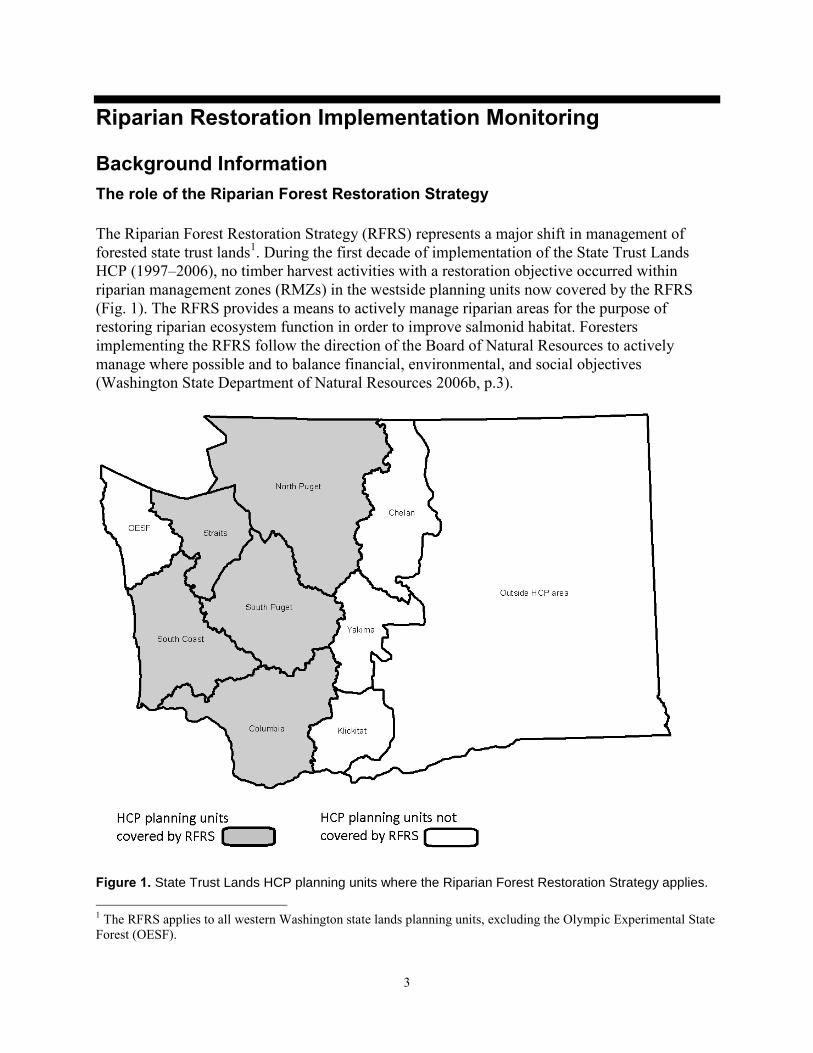
The Riparian Forest Restoration Strategy (RFRS) represents a major shift in management of forested state trust lands1. During the first decade of implementation of the State Trust Lands HCP (1997–2006), no timber harvest activities with a restoration objective occurred within riparian management zones (RMZs) in the westside planning units now covered by the RFRS (Fig. 1). The RFRS provides a means to actively manage riparian areas for the purpose of restoring riparian ecosystem function in order to improve salmonid habitat. Foresters implementing the RFRS follow the direction of the Board of Natural Resources to actively manage where possible and to balance financial, environmental, and social objectives (Washington State Department of Natural Resources 2006b, p.3).
Figure 1. State Trust Lands HCP planning units where the Riparian Forest Restoration Strategy applies.
1 The RFRS applies to all western Washington state lands planning units, excluding the Olympic Experimental State Forest (OESF).

4
Riparian Forest Restoration Strategy Monitoring The RFRS was approved in April 2006 (Washington State Department of Natural Resources 2006a). The strategy describes the ecological context, objectives, and sideboards to develop site-specific riparian forest prescriptions to achieve the Riparian Desired Future Conditions (RDFC; Table 1). It also defines minimum standards for prescriptions and specifies that ground-based equipment is not allowed within 50 feet of the 100-year floodplain. Table 1. Riparian Desired Future Conditions (RDFC) threshold targets (Washington State Department of
Natural Resources 2006a).
RDFC Characteristics RDFC Threshold Targets (Discrete Measurables) Basal area 300 sq. feet per acre
Quadratic mean diameter
(Trees >7 inches DBH)
21 inches
Snags Retain existing snags 20 inches DBH through no-cut zones
Maintain at least 3 snags per acre.
Large down wood Maintain 2,400 cubic feet/acre
Actively create down wood (contribute 5 trees from the largest thinned
DBH class) during each conifer management entry
Vertical stand structure Maintain at least two canopy layers (bimodal or developing reverse J-
shaped diameter distribution)
Species diversity Maintain at least two main canopy tree species suited to the site
Methods Monitoring the various components of the RFRS required the development of several distinct methodologies. The following is a summary of those methods; see Appendix 1 for a detailed description of the methods. We queried DNR databases and requested information from DNR staff to identify timber sales where riparian forest restoration activities were implemented between the approval of the RFRS in April 2006 and April 2012. Stream segments were identified from timber sales maps. Segments were considered those contiguous portions of a stream of one stream type between mapped stream type break points. Tributary forks were considered separate segments from the main stem of the stream. Stream segments were the sampling units for this project. We identified a total of 376 stream segments in 75 timber sales that implemented the RFRS timber harvest activities. We randomly selected 37 stream segments (9.8 percent) from this population for field review. Restoration thinning treatments occurred in the riparian management zones along 36 of the 37 segments visited, while hardwood conversion and individual conifer release activities were implemented on one of the 37 stream segments.
5
Our evaluation of field implementation of the RFRS was based on the criteria for management within the RMZs (Table 2). Along each stream segment, we measured the distance between the outer edge of the 100-year floodplain and the center of the nearest removed tree from this point. This area is called the inner zone in the RFRS. In addition, we measured and documented ground based equipment tracks if they were found within 50 feet of the outer edge of the 100-year floodplain (the equipment exclusion zone). We also measured the distance between the 100-year floodplain and the timber sale boundary tags to determine the area of the RMZ. When the RMZ was adjacent to an upland variable retention harvest, the distance to the special management boundary tags was also measured. Special management tags indicate a change in management activity, which, in RFRS areas, is a change from variable retention harvest to variable density thinning. The specifications for RMZ width are different between Type 3 and Type 4 streams. Along Type 3 streams the buffer must have an average width equal to the 100-year site index of the adjoining conifer stand as determined by following the appropriate procedure (PR 14-004-150, Identifying and Protecting Riparian and Wetland Management Zones in The Westside HCP Planning Units, Excluding the OESF (August 1999)). Along Type 4 streams a minimum 100-foot buffer must be maintained. We assessed the stream type for all sampled segments. We documented canopy gaps greater than 0.25 acre, if present. Salvage activities, which require site specific plans and approval by the HCP and Scientific Consultation Manager in consultation from the National Marine Fisheries Service and U.S. Fish and Wildlife Service, were not assessed in this monitoring project. In segments where restoration thinning treatments were implemented, we collected tree data using plots installed on a systematic grid within each buffer zone. Data from these plots were used to determine Curtis’ relative density, stem density, and the d/D ratio (d/D ratio is the ratio of the average diameter of cut trees to the average diameter of trees in the stand before harvest). Within each RMZ we tallied trees that were felled to create large woody debris (LWD), or intentionally damaged for the purpose of snag creation. The determination of whether a tree was counted as LWD was dependent on the prescription for LWD creation. We did not sample created LWD and snags but instead counted all LWD and snags along a segment. We intended to determine if five trees were cut for LWD or damaged to create snags for each acre of riparian restoration thinning. Logs were counted as LWD if they met certain search criteria. These criteria were different for sales where LWD was marked for creation and for sales where the operator selected trees for LWD. Along the former—segments where trees were marked to be felled for woody debris—we counted all marked trees that were cut or were planned to be cut prior to the completion of the sale. This protocol under-counted the number of trees left as woody debris where trees other than the marked trees were felled to create woody debris (i.e. in cases where trees were traded for operational reasons or where harvestable trees were cut but not removed). Along segments where trees were not marked to be felled for woody debris, we tallied only those trees which were felled in the direction of the stream. We did
6
not tally felled trees oriented away from the stream, or trees that did not appear to be intentionally left as woody debris (e.g., trees in log decks). In the stream segment managed for hardwood conversion and individual conifer release, we counted the number of viable conifers. Viable conifers are described in the RFRS as conifers greater than six inches in diameter at breast height, with live crowns more than 30 percent of total tree height, with height-to-diameter ratios less than 100, and free of root rot. We counted viable conifers to determine whether the segment met the eligibility requirements for these activities. We used multiple Student’s t-tests, adjusted using the Benjamini-Hochberg correction procedure for multiple hypothesis testing, to determine whether operations within sampled stream segments met or exceeded the residual density, stem density, and d/D ratio standards in the RFRS. A range of false discovery rates were used in the Benjamini-Hochberg correction procedure to assess the Student’s t-test results for each of the stand attributes. We calculated 95 percent confidence intervals (CI) for sample means to estimate the proportion of sales applying the RFRS that met or exceeded the standards in the RFRS for Curtis’ relative density (RD), stem density, and d/D ratio.
7
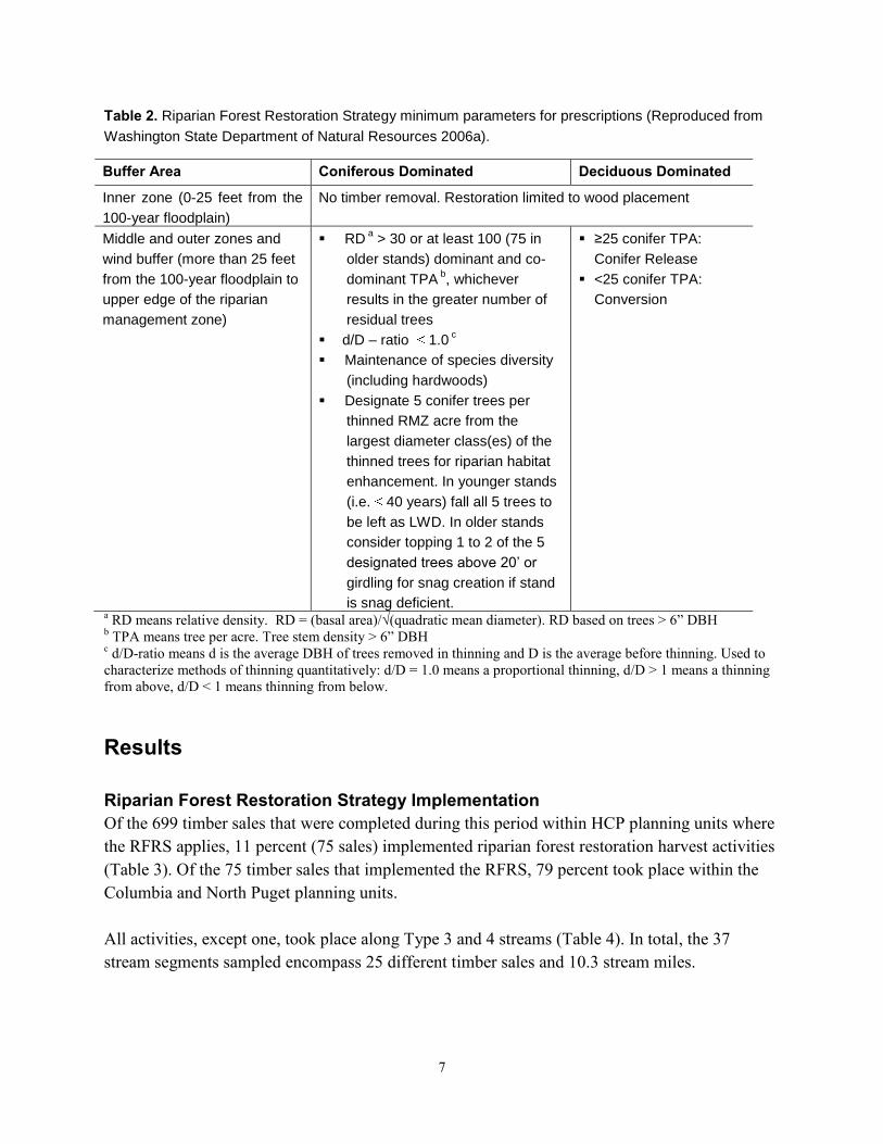
Table 2. Riparian Forest Restoration Strategy minimum parameters for prescriptions (Reproduced from
Washington State Department of Natural Resources 2006a).
Buffer Area Coniferous Dominated Deciduous Dominated
Inner zone (0-25 feet from the
100-year floodplain)
No timber removal. Restoration limited to wood placement
Middle and outer zones and
wind buffer (more than 25 feet
from the 100-year floodplain to
upper edge of the riparian
management zone)
RD a > 30 or at least 100 (75 in
older stands) dominant and co-
dominant TPA b, whichever
results in the greater number of
residual trees
d/D – ratio 1.0 c
Maintenance of species diversity
(including hardwoods)
Designate 5 conifer trees per
thinned RMZ acre from the
largest diameter class(es) of the
thinned trees for riparian habitat
enhancement. In younger stands
(i.e. 40 years) fall all 5 trees to
be left as LWD. In older stands
consider topping 1 to 2 of the 5
designated trees above 20’ or
girdling for snag creation if stand
is snag deficient.
≥25 conifer TPA:
Conifer Release
<25 conifer TPA:
Conversion
a RD means relative density. RD = (basal area)/√(quadratic mean diameter). RD based on trees > 6” DBH b TPA means tree per acre. Tree stem density > 6” DBH c d/D-ratio means d is the average DBH of trees removed in thinning and D is the average before thinning. Used to characterize methods of thinning quantitatively: d/D = 1.0 means a proportional thinning, d/D > 1 means a thinning from above, d/D < 1 means thinning from below. Results Riparian Forest Restoration Strategy Implementation
Of the 699 timber sales that were completed during this period within HCP planning units where the RFRS applies, 11 percent (75 sales) implemented riparian forest restoration harvest activities (Table 3). Of the 75 timber sales that implemented the RFRS, 79 percent took place within the Columbia and North Puget planning units. All activities, except one, took place along Type 3 and 4 streams (Table 4). In total, the 37 stream segments sampled encompass 25 different timber sales and 10.3 stream miles.
8
Table 3. Number of timber sales and stream segments with riparian restoration activities by planning unit.
Planning Unit
Number of stream segments within RFRS implementation units
Number of timber sales with RFRS implementation
Total number timber sales completed April 2006 to April 2012
Sales with RFRS implementation (%)
Columbia 139 31 153 20%
North Puget 163 28 221 13%
South Coast 29 6 187 3%
South Puget 45 10 64 16%
Straits 0 0 74 0%
Total 376 75 699 11%
Table 4. Number of stream segments with riparian restoration by stream type.
Stream type Number of segments with riparian restoration
Type 1 1
Type 2 0
Type 3 161
Type 4 214
Total 376
The mean size of the riparian management zones sampled was 3.6 acres. The 95 percent confidence interval (CI)2 of the mean size of riparian restoration units was 2.3 to 4.8 acres. Based on this, an estimated 1,340 acres (95 percent CI 882 – 1798 acres) were treated under the RFRS between April 2006 and April 2012. Over the same period, timber sale activities were completed (closed in DNR’s revenue tracking system) on 89,826 acres across state lands in the westside planning units excluding the OESF. Riparian restoration activities accounted for an estimated 1 percent to 2 percent of the total harvest area.
Thinning operations
Post treatment stem densities (measured in trees per acre, TPA) and leave tree size selection (d/D ratio) along all 36 sampled segments where thinning activities were implemented met or exceeded the target based on our statistical analysis (Table 5). While seven segments had average TPA less than the target level of 75 or 100 TPA (depending on thinning type), these results were not statistically significant due to variability in the stand and sampling intensity. Six segments had average d/D ratios greater than 1.0, but again, these results were not statistically 2 The confidence interval is a statistical description of the certainty of the reported success rate. In this case, it is expected that 19 out of 20 similar samples would return mean success rates in this range.
9
significant. While a total of eight stream segments had a RD less than the target level of 35, only one of these results was statistically significant (segment mean RD = 24.5, p = 5.3 x 10⁻⁷). This segment was the only segment found to have significantly lower RD than the target at any significance threshold used. We were unable to determine why this segment had an RD below the target. The statewide success rate and confidence intervals for each attribute was estimated from these results (Table 5). The mean RD in sampled segments ranged from 25 to 65, with a mean of 43. Table 5. Estimated statewide success rate and 95 percent confidence interval for implementation of restoration thinning activities by stand attribute.
Stand attribute Estimated statewide success rate
95% confidence interval of success rate
Trees per acre 100 89 – 100
d/D ratio 100 89 – 100
Relative density 97 84 – 100
Hardwood conversion/individual conifer release
The hardwood conversion and individual conifer release operations were done in appropriate areas based on the number of viable residual conifers and the lack of conifer stumps, as harvesting of conifers is not allowed unless operational or safety needs require their removal. More than 25 well-established conifers per acre were found in the individual conifer release section of the segment, while fewer than 25 well-established conifers per acre were found in the hardwood conversion section of the segment.
Distance to harvest operations
Across all 37 segments visited, a total of 12 trees were found removed from within 25 feet of the outer edge of the 100-year floodplain (Table 6). The 12 trees came from 5 of the 37 segments sampled. For all of the segments, this equates to the removal of 1.17 trees per mile of riparian restoration. In each case, the cut trees were within the marked timber sales boundary. Table 6. Distance to trees removed from within 25 feet of the outer edge of the 100-year floodplain.
Distance from outer edge of 100 year floodplain
Number of trees removed
20 to < 25 feet 5
10 to < 20 feet 5
< 10 feet 2
Total 12
10
Distance to machine entry
Five instances of machine entry into the equipment exclusion zone were found (Table 7). These entries were found along four different segments. For all the segments, this results in a machine entry rate of 0.49 entries per mile of riparian restoration. No evidence of delivery of sediment to the stream was seen associated with these entries.
Table 7. Distance to machine tracks within 50 feet of the 100-year floodplain.
Distance from edge 100 year floodplain to nearest machine entry
Number of entries
40 to < 50 feet 2
30 to < 40 feet 3
< 30 feet 0
Total 5
Distance to special management unit tags
The difference in riparian buffer width requirements for Type 3 (average 100-year site index) and Type 4 streams (minimum 100 feet) necessitated different approaches to riparian management zone width data interpretation. We next address the width and variability of the observed buffers. Type 3 streams – Measurements of distance to the special management unit tags showed all eight Type 3 streams had buffers equal to or exceeding the required buffer within the measurement error of the tools used to measure distance (Fig. 3). Two of the segments had buffers greater than 70-feet wider than required. At one segment this was possibly due to the presence of a low river terrace above the 100-year floodplain. We suspect this terrace was misidentified as the 100-year floodplain and that the buffer was measured from the point where this terrace meets the upland hillslope. The other segment had no identifiable feature that could explain the additional buffering. Type 4 streams- The average distance to the special management unit tags on all four of these streams was greater than 100 feet. However, along all segments 19 percent to 43 percent of measurements to the special management unit tags were less than 100 feet. The distance to the first stump beyond the special management unit tags was not measured. Without these data, further analysis was not possible. RMZ width variability - Riparian management zone buffer widths along Type 3 streams were highly variable. Along Type 3 streams, the difference between the narrowest and widest buffer width measurements on a given segment ranged from 18 percent to 71 percent of the mean buffer width of the segment.
11
No canopy gaps greater than 0.25 acre were found in any segment within 100 feet of the 100-year floodplain.
Figure 2. Difference between the mean measured buffer and the required buffer on segments with Type
3 streams.
* Note: The difference between the mean measured buffer and the required buffer was -1 feet, which is within the margin of error of the laser range finder used to measure the buffer width.
Stream typing
We found that the stream typing indicated in the timber sale documents matched our stream type assessments for 31 stream segments. On the other six stream segments we found typing differences between the monitoring assessment and the timber sale documents (Table 8). All six of these stream segments were adjacent to upland variable density thinning operations where there is no difference in RMZ procedure between Type 1, 2, 3, and 4 streams.
0
1
2
3
4
5
6
7
8
9
10
Nu
mb
er o
f se
gmen
ts
Feet
*
12
Table 8. Comparison of stream types in timber sale documents and on-site post-sale stream type
measurements and determinations.
Number of streams
Description of results
31 Pre and Post treatment stream type matched: Stream type listed on timber sale map
matched that found by the implementation monitoring team.
1
Under-typed: Listed as Type 4 stream, but Type 3 physical attributes continued 950
feet beyond the mapped Type break and fish were present for more than 500 feet.
However, since the upland harvest was a variable density thinning, the same
procedure applies to both Type 3 and Type 4 streams. Harvesting that occurred is
within the guidelines.
2
Under-typed: Listed as Type 4 streams, but sections less than or equal to 350 feet at
the downstream end of these segments had Type 3 physical attributes. No fish were
observed. Since the upland harvests were variable density thinning operations, the
same procedure applies to both Type 3 and Type 4 streams. Harvesting that
occurred is within the guidelines.
1
Over-typed: Listed as Type 4 stream, but the upper section of segment had Type 5
physical attributes for 600 feet. The upland harvest was a variable density thin so
over-typing did not reduced the volume of wood harvested.
1
Over-typed: Listed as Type 3 stream, but the upper section of segment had Type 5
physical attributes for 300 feet. The upland harvest was a variable density thin so
over-typing did not reduced the volume of wood harvested.
1
Inconclusive: Listed as a Type 4 stream, but the upper section of segment had Type
5 physical attributes for 200 feet to a culvert at the edge of the timber sale. The
stream continues several hundred feet up stream from the culvert but no data were
collected on this part of the stream.
Large woody debris/snags
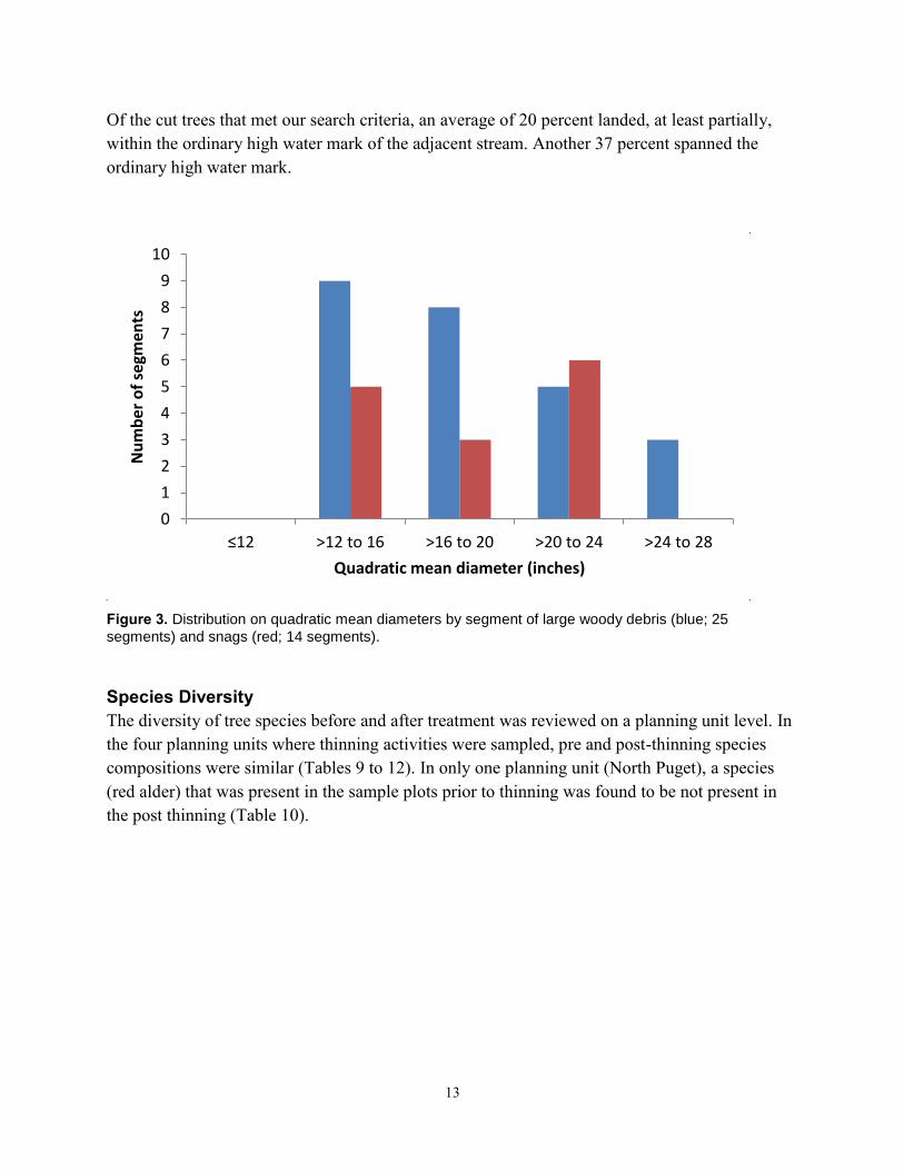
Results for snag and woody debris creation were mostly inconclusive. The methods used to measure the implementation of the large wood debris component of the RFRS did not capture all the woody debris that was created during treatment. Eight segments were found to have at least 100 percent of the required large woody debris (5 trees per thinned RMZ acre). Excluding the smallest segments, those under one acre, six sales have over 100 percent of the requirement. Three segments larger than one acre did not have any woody debris that met our search criteria. Snags were created along 41 percent of segments. Snag density in these segments ranged from 0.2 to 9.5 per acre. The quadratic mean diameter3 (QMD) of large woody debris ranged from 12.6 to 27.3 inches (Fig. 4). The QMD of snags ranged from 12.1 inches to 23.5 inches.
3 Quadratic mean diameter equals the square root of the mean of the squared diameters of trees in a stand. The equation is: QMD= , where Di is the diameter of the ith tree and n is the number of trees.
13
Of the cut trees that met our search criteria, an average of 20 percent landed, at least partially, within the ordinary high water mark of the adjacent stream. Another 37 percent spanned the ordinary high water mark.
Figure 3. Distribution on quadratic mean diameters by segment of large woody debris (blue; 25
segments) and snags (red; 14 segments).
Species Diversity
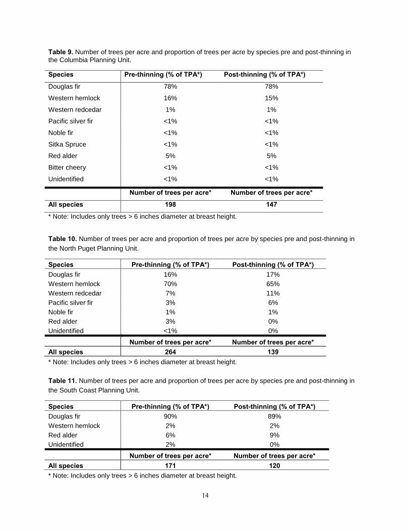
The diversity of tree species before and after treatment was reviewed on a planning unit level. In the four planning units where thinning activities were sampled, pre and post-thinning species compositions were similar (Tables 9 to 12). In only one planning unit (North Puget), a species (red alder) that was present in the sample plots prior to thinning was found to be not present in the post thinning (Table 10).
0
1
2
3
4
5
6
7
8
9
10
≤12 >12 to 16 >16 to 20 >20 to 24 >24 to 28
Nu
mb
er o
f se
gmen
ts
Quadratic mean diameter (inches)
14
Table 9. Number of trees per acre and proportion of trees per acre by species pre and post-thinning in
the Columbia Planning Unit.
Species Pre-thinning (% of TPA*) Post-thinning (% of TPA*)
Douglas fir 78% 78%
Western hemlock 16% 15%
Western redcedar 1% 1%
Pacific silver fir <1% <1%
Noble fir <1% <1%
Sitka Spruce <1% <1%
Red alder 5% 5%
Bitter cheery <1% <1%
Unidentified <1% <1%
Number of trees per acre* Number of trees per acre*
All species 198 147
* Note: Includes only trees > 6 inches diameter at breast height.
Table 10. Number of trees per acre and proportion of trees per acre by species pre and post-thinning in
the North Puget Planning Unit.
Species Pre-thinning (% of TPA*) Post-thinning (% of TPA*) Douglas fir 16% 17%
Western hemlock 70% 65%
Western redcedar 7% 11%
Pacific silver fir 3% 6%
Noble fir 1% 1%
Red alder 3% 0%
Unidentified <1% 0%
Number of trees per acre* Number of trees per acre* All species 264 139 * Note: Includes only trees > 6 inches diameter at breast height.
Table 11. Number of trees per acre and proportion of trees per acre by species pre and post-thinning in
the South Coast Planning Unit.
Species Pre-thinning (% of TPA*) Post-thinning (% of TPA*) Douglas fir 90% 89%
Western hemlock 2% 2%
Red alder 6% 9%
Unidentified 2% 0%
Number of trees per acre* Number of trees per acre* All species 171 120 * Note: Includes only trees > 6 inches diameter at breast height.
15
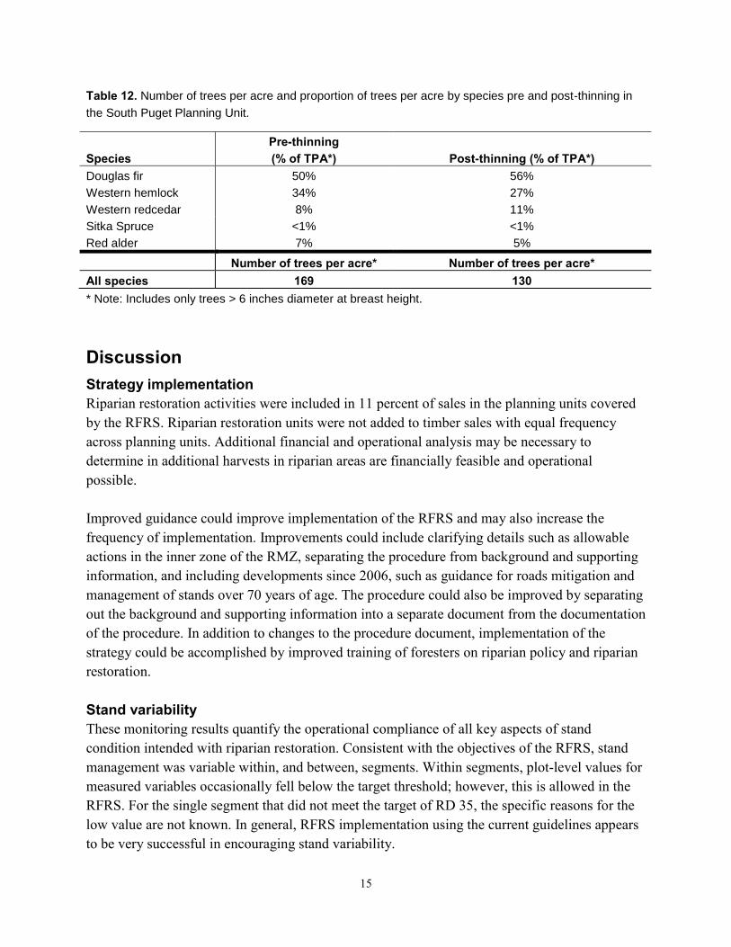
Table 12. Number of trees per acre and proportion of trees per acre by species pre and post-thinning in
the South Puget Planning Unit.
Species
Pre-thinning (% of TPA*) Post-thinning (% of TPA*)
Douglas fir 50% 56%
Western hemlock 34% 27%
Western redcedar 8% 11%
Sitka Spruce <1% <1%
Red alder 7% 5%
Number of trees per acre* Number of trees per acre* All species 169 130 * Note: Includes only trees > 6 inches diameter at breast height.
Discussion Strategy implementation
Riparian restoration activities were included in 11 percent of sales in the planning units covered by the RFRS. Riparian restoration units were not added to timber sales with equal frequency across planning units. Additional financial and operational analysis may be necessary to determine in additional harvests in riparian areas are financially feasible and operational possible. Improved guidance could improve implementation of the RFRS and may also increase the frequency of implementation. Improvements could include clarifying details such as allowable actions in the inner zone of the RMZ, separating the procedure from background and supporting information, and including developments since 2006, such as guidance for roads mitigation and management of stands over 70 years of age. The procedure could also be improved by separating out the background and supporting information into a separate document from the documentation of the procedure. In addition to changes to the procedure document, implementation of the strategy could be accomplished by improved training of foresters on riparian policy and riparian restoration. Stand variability
These monitoring results quantify the operational compliance of all key aspects of stand condition intended with riparian restoration. Consistent with the objectives of the RFRS, stand management was variable within, and between, segments. Within segments, plot-level values for measured variables occasionally fell below the target threshold; however, this is allowed in the RFRS. For the single segment that did not meet the target of RD 35, the specific reasons for the low value are not known. In general, RFRS implementation using the current guidelines appears to be very successful in encouraging stand variability.
16
Limiting operations near streams
The equipment exclusion zone specific to the RFRS (50 feet) is wider than the Forest Practices equipment limitation zone (30 feet). This may cause confusion amongst foresters and operators. Making the RFRS procedures more accessible, and highlighting the particular specifications of the strategy in presales briefings would help ensure proper use of machines in riparian management zones. Management within the inner zone (25 feet of the 100-year floodplain) is limited to LWD creation and site specific low-impact thinnings (see Table 2). We found several instances where LWD trees were cut and remained as LWD. The five trees we measured may have been intended as LWD, but were subsequently removed. No markings remained on site to further interpret the intention of the tree cutting and no information was available in the timber sale packet. The RFRS procedure inconsistently states whether trees can be cut within the inner zone for LWD creation. Table 2 shows that LWD can be created in the inner zone. In another part of the strategy it states that this is not allowed (Washington State Department of Natural Resources 2006a, p. 26). Ensuring that strategy guidance is consistently and clearly stated will be useful in reducing confusion and improving implementation of the RFRS on the ground.
Large wood debris
The method for counting large woody debris and snags under-represented the total number of trees cut for woody debris. Because of this, it was not possible to fully assess the implementation of this portion of the RFRS. In addition, since LWD can be created anywhere in the operable riparian area, it is possible that adequate woody debris was left in riparian areas outside of the sample segments. For, example enough LWD may have been left in other parts of the timber sales that included the three segments of more than one acre in size that showed no evidence of created LWD. In the future, crews monitoring LWD creation in riparian areas should consider using different methods than those used here. Hardwood conversion/ individual conifer release
We sampled one segment that implemented both hardwood conversion and individual conifer release activities. We found that both activities were implemented in appropriate areas based on the number of confers in the RMZ. Continued emphasis on proper site selection for thinning and tracking of treated sites will ensure proper implementation of this component of the RFRS in the future. Stream typing and buffer application
Stream location and typing is a difficult aspect of timber sales. Although we took only a small sample, we found our stream typing to be consistent with timber sale documents on 31 of 37 segments. Where stream typing discrepancies appeared to occur, correct buffers were maintained

17
on the streams due to the implementation of upland thinning activities. Nonetheless, correct stream typing is crucial to the successful implementation of the Riparian Conservation Strategy for the Five Westside Planning Units, of which the RFRS is a part. Correct stream typing is also necessary to fulfill the Multispecies Conservation Strategy for Unlisted Species in the Five Westside Planning Units because implementation of the riparian strategy, along with the northern spotted owl and marbled murrelet strategies, is part of the multispecies conservation strategy. Based on meetings with regional DNR staff about the results of this assessment, we recommend that additional training on the stream typing procedure be provided to foresters. Increased stream typing training has the potential to greatly increase the efficiency and effectiveness of HCP strategy implementation, while also reducing the risks associated with the mistyping of streams. One area where training could provide clarity to foresters is the typing of lower portions of tributary streams that are less than 500 feet long and which have the physical attributes of a Type 3 or 4 stream but the upper reaches of the stream have Type 4 or 5 attributes.
The implementation monitoring pilot project in 2002 reported that stream typing was correct for 92 percent of streams assessed. Our data showed that 84 percent of streams were typed the same by the pre-sales foresters and the monitoring team. Increased training may be necessary to improve stream typing accuracy.
RMZ width
The RMZ width is the horizontal distance between the edge of the 100-year floodplain and the upland harvest area. Several aspects of the identification of the 100-year floodplain are subjective, including location of the ordinary high water mark, and location of stream depth measurements. While subjectivity makes it difficult to identify errors, major misidentification of the ordinary high water mark and other errors are possible. These errors can result in inconsistent implementation, such as inappropriately sized buffers. In 2006, The Implementation Monitoring Program reviewed the width of unmanaged RMZ buffers. They found that 82 percent of buffers were equal to or greater in width than required. The implementation monitoring pilot project in 2002 reported that 75 percent of buffers assessed were adequately sized. The 100 percent rate of compliance in Type 3 RMZ width we found compares favorably to the previous results. Additional data is needed to assess Type 4 RMZ widths. One area where improvement is needed is in documenting very large RMZs: the two segments we sampled with RMZs more than 70 feet wider than the minimum did not have any documentation of the purpose of the extended buffers. We measured RMZ widths using laser rangefinders and, occasionally, when sightlines were obstructed, 75-foot loggers’ tapes. These tools are available to foresters setting up timber sales.
18
Instead of these tools, some foresters use Global Positioning System (GPS) units to measure buffer distances. We do not know what tools foresters used to measure the width of the buffers we reviewed. Species Diversity
Thinning activities maintained existing conifer diversity in all planning units. Red alder was removed from sample plots in one planning unit. However, its removal may have been appropriate to ensure the development of a two-storied stand as defined in the RDFC. Also, the finding that red alder was not present in the post-harvest plots in one planning unit does not necessarily indicated that it was removed from adjacent riparian area or even the harvest unit.

19
Potentially Unstable Hillslope Management Implementation Monitoring
Background information
The role of the unstable hillslope components
Management of potentially unstable hillslopes is included in the HCP in both the Riparian Conservation Strategy for the Five Westside Planning Units and the Riparian Conservation Strategy for the Olympic Experimental State Forest (Fig. 5). For the five westside planning units the HCP sets the goal of accomplishing timber harvest and related activities, such as road building, without increasing the frequency or severity of slope failure and without altering the natural input of large woody debris, sediment, and nutrients to the stream network. For the Olympic Experimental State Forest (OESF) Planning Unit, the HCP states an objective of maintaining and aiding restoration of the integrity of stream channels and the natural disturbance and sediment regimes of streams. While the specific methods used to manage potentially unstable hillslopes may differ by site, the same potentially unstable landforms are identified in the pre-sale review process in five westside and OESF planning units.
20
Figure 4. State Trust Lands HCP planning units where unstable hillslope components are implemented.
Methods Implementation monitoring of the potentially unstable hillslope components included both office and field review. The following is a summary of the methods used in the office review and the complete methods for the field review; see Appendix 2 for a detailed description of the methods used in the office review. Office review consisted of a review of timber sale documents and relevant geographic information system layers by implementation monitoring staff. All timber sales completed (i.e. closed in DNR’s revenue tracking program) in fiscal year 2012 were reviewed. Earth Sciences Program staff conducted the field reviews. Earth sciences staff members made a follow-up visit to 10 projects that they had visited during the pre-work period. These projects were distributed throughout the state trust lands covered by the unstable hillslope components of the HCP. The 10 projects were specifically, not randomly, selected because they were areas with challenging slope stability issues identified during the pre-work process. Specific selection was
21
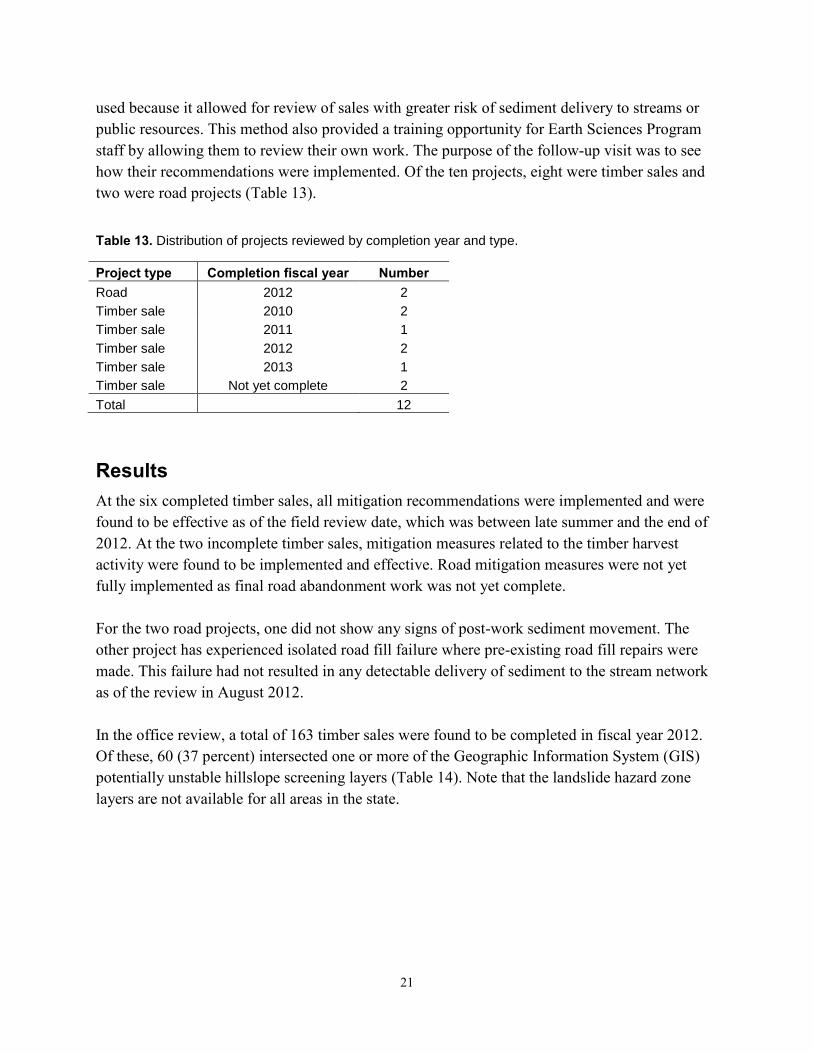
used because it allowed for review of sales with greater risk of sediment delivery to streams or public resources. This method also provided a training opportunity for Earth Sciences Program staff by allowing them to review their own work. The purpose of the follow-up visit was to see how their recommendations were implemented. Of the ten projects, eight were timber sales and two were road projects (Table 13).
Table 13. Distribution of projects reviewed by completion year and type.
Project type Completion fiscal year Number Road 2012 2
Timber sale 2010 2
Timber sale 2011 1
Timber sale 2012 2
Timber sale 2013 1
Timber sale Not yet complete 2
Total 12
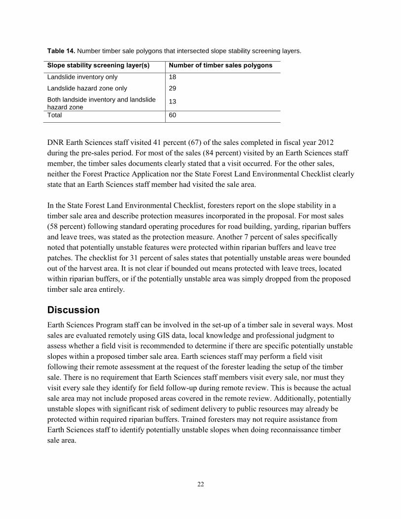
Results At the six completed timber sales, all mitigation recommendations were implemented and were found to be effective as of the field review date, which was between late summer and the end of 2012. At the two incomplete timber sales, mitigation measures related to the timber harvest activity were found to be implemented and effective. Road mitigation measures were not yet fully implemented as final road abandonment work was not yet complete. For the two road projects, one did not show any signs of post-work sediment movement. The other project has experienced isolated road fill failure where pre-existing road fill repairs were made. This failure had not resulted in any detectable delivery of sediment to the stream network as of the review in August 2012. In the office review, a total of 163 timber sales were found to be completed in fiscal year 2012. Of these, 60 (37 percent) intersected one or more of the Geographic Information System (GIS) potentially unstable hillslope screening layers (Table 14). Note that the landslide hazard zone layers are not available for all areas in the state.
22
Table 14. Number timber sale polygons that intersected slope stability screening layers.
Slope stability screening layer(s) Number of timber sales polygons
Landslide inventory only 18
Landslide hazard zone only 29
Both landside inventory and landslide hazard zone
13
Total 60
DNR Earth Sciences staff visited 41 percent (67) of the sales completed in fiscal year 2012 during the pre-sales period. For most of the sales (84 percent) visited by an Earth Sciences staff member, the timber sales documents clearly stated that a visit occurred. For the other sales, neither the Forest Practice Application nor the State Forest Land Environmental Checklist clearly state that an Earth Sciences staff member had visited the sale area. In the State Forest Land Environmental Checklist, foresters report on the slope stability in a timber sale area and describe protection measures incorporated in the proposal. For most sales (58 percent) following standard operating procedures for road building, yarding, riparian buffers and leave trees, was stated as the protection measure. Another 7 percent of sales specifically noted that potentially unstable features were protected within riparian buffers and leave tree patches. The checklist for 31 percent of sales states that potentially unstable areas were bounded out of the harvest area. It is not clear if bounded out means protected with leave trees, located within riparian buffers, or if the potentially unstable area was simply dropped from the proposed timber sale area entirely. Discussion Earth Sciences Program staff can be involved in the set-up of a timber sale in several ways. Most sales are evaluated remotely using GIS data, local knowledge and professional judgment to assess whether a field visit is recommended to determine if there are specific potentially unstable slopes within a proposed timber sale area. Earth sciences staff may perform a field visit following their remote assessment at the request of the forester leading the setup of the timber sale. There is no requirement that Earth Sciences staff members visit every sale, nor must they visit every sale they identify for field follow-up during remote review. This is because the actual sale area may not include proposed areas covered in the remote review. Additionally, potentially unstable slopes with significant risk of sediment delivery to public resources may already be protected within required riparian buffers. Trained foresters may not require assistance from Earth Sciences staff to identify potentially unstable slopes when doing reconnaissance timber sale area.
23
In the remote review process Earth Sciences staff may assess, among other things, information in the landside hazard zone and the landslide inventory layers in a geographic information system. The landslide hazard zone layers are a set of mapped data layers showing instability potential. The layers have not been prepared for all areas in the state. The landslide inventory shows mapped landslides and suspected landslides. Neither of these layers has been rigorously field verified. Because of this, intersection between timber sale polygons and polygons within one of these layers does not automatically result in mitigation activities being warranted. Field verification needs to be completed to determine the need for mitigation. If a field visit is completed by Earth Sciences staff, it is useful to record this in the State Forest Land Environmental Checklist submitted as part of the State Environmental Policy Act review process. Doing this will help record how slope stability concerns have been addressed.
24
Appendix 1: Detailed methods for Riparian restoration monitoring
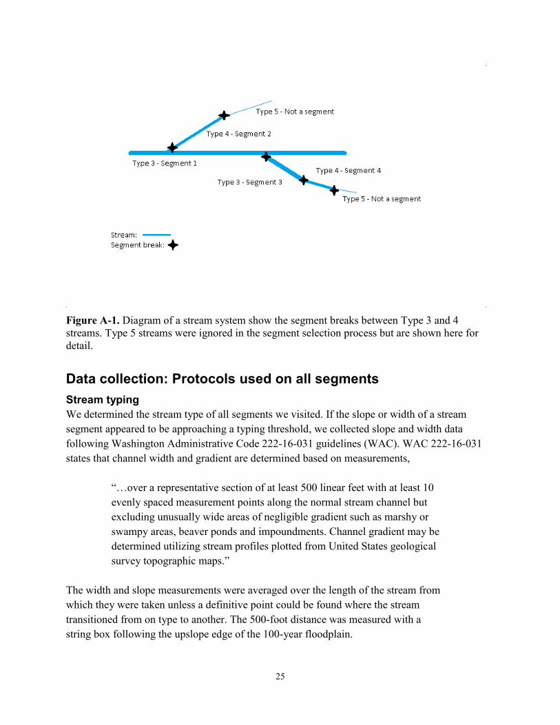
Timber sale identification We identified sales that implemented or planned to implement the Riparian Forest Restoration Strategy between April 2006 and April 2012 by querying DNR’s Forest Management Planning and Tracking database and reviewing staff work files. These dates encompass the entire periods between the introduction of the RFRS and the last complete month before the query was made. We queried Planning and Tracking to find forest management units with “riparian” in the objective category. Then we queried a Geographic Information System layer, which is compiled from data in Planning and Tracking, for forest management units with names that began or ended with “RR,” “RFRS,” or “RMZ.” Once we identified these units, we reviewed the prescriptions to verify that riparian restoration was planned or had been implemented. Finally, we reviewed spreadsheets provided by Forest Resource and Conservation Division, and Northwest Region staffs listing sales where riparian restoration activities had occurred. The resulting list of sales included salvage sales, which were dropped from the list because no general procedure is approved for these sales. Each salvage sale requires a site-specific plan and special approval. In all, 75 timber sales included riparian restoration units that were not salvage operations. Sampling unit The sampling unit in this project was a ‘stream segment.’ A stream segment was a portion of a Type 1, 2, 3, or 4 stream adjacent to a riparian restoration activity identified on a timber sale map in the packets stored in the Timber Sale Document Center or in Forest Resources and Conservation Division electronic files. Segments ended where the stream type changed, or at the edge of the timber sale. When a stream forked into two streams of the same type, we gave a new segment number to the stream that appeared to have the smallest basin based on the information on the timber sale map. We assumed that streams shown to be shorter, have fewer tributaries, and/or branch sharply from the direction of stream below the fork have a smaller basin (Fig. A-1). In all, 376 stream segments were identified. We recorded each segment in a spreadsheet and gave it an ID number. We assessed 37 randomly selected segments.
25
Figure A-1. Diagram of a stream system show the segment breaks between Type 3 and 4 streams. Type 5 streams were ignored in the segment selection process but are shown here for detail.
Data collection: Protocols used on all segments Stream typing
We determined the stream type of all segments we visited. If the slope or width of a stream segment appeared to be approaching a typing threshold, we collected slope and width data following Washington Administrative Code 222-16-031 guidelines (WAC). WAC 222-16-031 states that channel width and gradient are determined based on measurements,
“…over a representative section of at least 500 linear feet with at least 10 evenly spaced measurement points along the normal stream channel but excluding unusually wide areas of negligible gradient such as marshy or swampy areas, beaver ponds and impoundments. Channel gradient may be determined utilizing stream profiles plotted from United States geological survey topographic maps.”
The width and slope measurements were averaged over the length of the stream from which they were taken unless a definitive point could be found where the stream transitioned from on type to another. The 500-foot distance was measured with a string box following the upslope edge of the 100-year floodplain.
26
Distance to tree tags and to operations
At 50-foot intervals, we measured the horizontal distance from the upper edge of the 100-year floodplain to the timber sale boundary tags and to the center of the stump of the first removed tree. We identified the 100-year floodplain visually based on channel morphology and topography, or, if the location of the upper edge of the 100-year floodplain was difficult to determine visually, following Procedure 14-004-150. This procedure entails first identifying the stream channel ordinary high water mark and then dividing the channel into 4 or more equal sections. At the edge of each section a measurement is taken from the elevation of the ordinary high water mark to the bottom of the channel. The elevation of upper edge of the 100-year floodplain is found by adding the mean of the measurements to the elevation of ordinary high water mark. This elevation is then found on the stream bank. We measured the horizontal distance to the timber sale boundary from the 100-year floodplain to the center of trees marked with timber sale boundary tags or pink flagging, depending on the marking protocol used, or a point situated on a straight line between marked trees. We considered the distance from the upper edge of the 100-year floodplain to the center of the first cut tree or the edge of ground disturbance by ground based harvesting equipment to be the operations distance. If the edge of operations is more than 50 feet from the upper edge of the 100-year floodplain, recorded ’50.’ When no timber sale boundary tags were found only the distance to the edge of operations was measured. Machine exclusion zone
The integrity of the 50-foot machine exclusion zone was assessed. We took horizontal distance measurements to machine activity whenever machine activity was found within 50 feet of the upper edge of the 100-year floodplain. Data collection: Additional protocol for riparian thinning units We collected data in variable and fixed radius plots to find Curtis’ relative density, stem density, and the d/D ratio (the ratio the average diameter of trees removed in thinning to the average prior to thinning). We used either basal area factor 20 or 40 prisms for the variable radius plots. The fixed radius plots had radii of either 16.7 feet or 21.5 feet, for areas of 1/50th and 1/30th acre, respectively. We selected the plot sizes to use based on the stand conditions along each segment. We measured the diameter at breast height and recorded the species of all trees within the fixed and variable radius plots greater than six inches at breast height. The fixed radius plot served as a search area for stumps. For each stump shorter than breast height (4.5 feet) within the fixed radius plot, we measured the inside bark diameter. We measured stumps taller than 4.5 feet at breast height outside the bark.
27
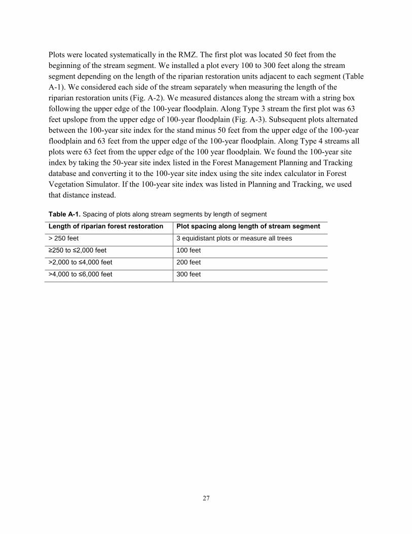
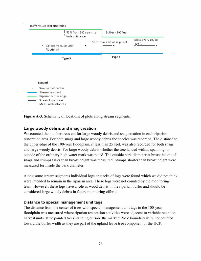
Plots were located systematically in the RMZ. The first plot was located 50 feet from the beginning of the stream segment. We installed a plot every 100 to 300 feet along the stream segment depending on the length of the riparian restoration units adjacent to each segment (Table A-1). We considered each side of the stream separately when measuring the length of the riparian restoration units (Fig. A-2). We measured distances along the stream with a string box following the upper edge of the 100-year floodplain. Along Type 3 stream the first plot was 63 feet upslope from the upper edge of 100-year floodplain (Fig. A-3). Subsequent plots alternated between the 100-year site index for the stand minus 50 feet from the upper edge of the 100-year floodplain and 63 feet from the upper edge of the 100-year floodplain. Along Type 4 streams all plots were 63 feet from the upper edge of the 100 year floodplain. We found the 100-year site index by taking the 50-year site index listed in the Forest Management Planning and Tracking database and converting it to the 100-year site index using the site index calculator in Forest Vegetation Simulator. If the 100-year site index was listed in Planning and Tracking, we used that distance instead. Table A-1. Spacing of plots along stream segments by length of segment
Length of riparian forest restoration Plot spacing along length of stream segment
> 250 feet 3 equidistant plots or measure all trees
≥250 to ≤2,000 feet 100 feet
>2,000 to ≤4,000 feet 200 feet
>4,000 to ≤6,000 feet 300 feet
28
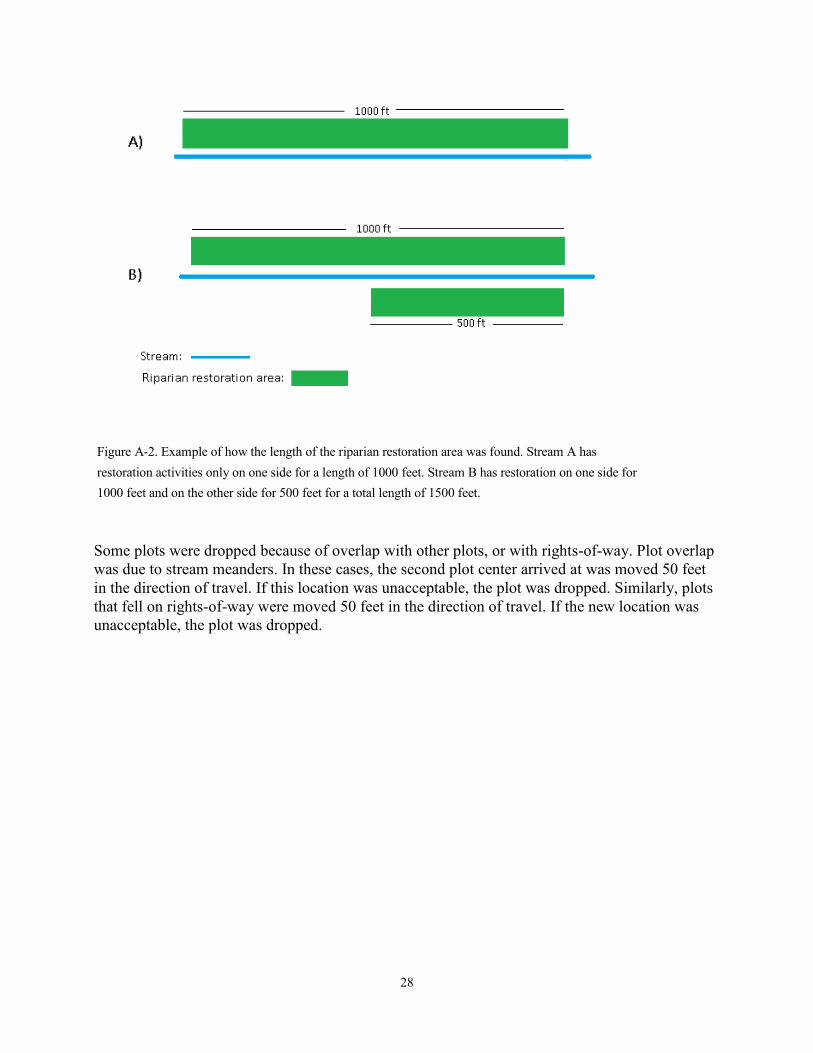
Figure A-2. Example of how the length of the riparian restoration area was found. Stream A has restoration activities only on one side for a length of 1000 feet. Stream B has restoration on one side for 1000 feet and on the other side for 500 feet for a total length of 1500 feet.
Some plots were dropped because of overlap with other plots, or with rights-of-way. Plot overlap was due to stream meanders. In these cases, the second plot center arrived at was moved 50 feet in the direction of travel. If this location was unacceptable, the plot was dropped. Similarly, plots that fell on rights-of-way were moved 50 feet in the direction of travel. If the new location was unacceptable, the plot was dropped.
29
Figure A-3. Schematic of locations of plots along stream segments.
Large woody debris and snag creation
We counted the number trees cut for large woody debris and snag creation in each riparian restoration area. For both snags and large woody debris the species was recorded. The distance to the upper edge of the 100-year floodplain, if less than 25 feet, was also recorded for both snags and large woody debris. For large woody debris whether the tree landed within, spanning, or outside of the ordinary high water mark was noted. The outside bark diameter at breast height of snags and stumps taller than breast height was measured. Stumps shorter than breast height were measured for inside the bark diameter. Along some stream segments individual logs or stacks of logs were found which we did not think were intended to remain in the riparian area. These logs were not counted by the monitoring team. However, these logs have a role as wood debris in the riparian buffer and should be considered large woody debris in future monitoring efforts. Distance to special management unit tags
The distance from the center of trees with special management unit tags to the 100-year floodplain was measured where riparian restoration activities were adjacent to variable retention harvest units. Blue painted trees standing outside the marked RMZ boundary were not counted toward the buffer width as they are part of the upland leave tree component of the HCP.
30
Canopy gaps
We looked for canopy gaps greater than 0.25 acre. Canopy gaps were measured following the drip lines of adjacent trees. Data collection: Additional protocol for hardwood conversion units Hardwood conversion units were assessed to determine whether fewer than 25 viable conifers per acre were present within a unit and that no conifers were removed, unless their removal was necessary for operational reasons. As the patch size of hardwood conversion units was small, we surveyed the entire units. The survey entailed counting the number of viable conifers. If we could not determine the viability of a tree visually, measurements of the height, the height to base of live crown, and the presence or absence of root rot in conifers greater than 6 inches diameter at breast height were recorded. We also tallied big-leaf maple trees in the stand. Additional data we collected included the latitude and longitude of the boundaries of the unit, and the distance up or downstream to the next hardwood conversion unit, where applicable. Data collection: Additional protocol Individual conifer release At individual conifer release units we determined whether more than 25 viable conifers per acre were present and that no conifers were removed, unless necessarily for operational reasons. We surveyed entire individual conifer release units because of their small size. The survey entailed counting the number of viable conifers. If we could not determine the viability of a tree visually, measurements of the height, the height to base of live crown, and the presence or absence of root rot in conifers greater than six inches diameter at breast height were recorded. Additionally, we recorded the latitude and longitude of the boundaries of the units. Equipment Distance measurements were taken with laser range finders or a 75-foot metal logger’s tape to the nearest foot. Two different laser range finders were used. One, the Laser Technology TruPulse 360 R, has typical a distance accuracy rating of ±1 foot. The other, the Laser Technology Impulse 200 R, has a typical distance accuracy rating of ±0.2 foot. A loggers tape was also used to take diameter measurements to the nearest 0.1 inch. Percent slope was measured using a Suunto clinometer to the nearest 1 percent. Data collection period Data were collected between July 16 and October 3, 2012.
31
Analysis We entered data from field datasheets into an Access database. Access, Excel and R (R Development Core Team 2011) were used to calculate descriptive statistics. Statistically significant differences between the mean diameter of stumps and the mean diameter of trees in the stand before harvest (i.e. the d/D ratio) were found using one-sided two-sample t-tests. One-sided one-sample t-tests were used to determine if the relative density in each segment was significantly below 35 and if stem density was significantly below 75 or 100 trees per acre, depending on the density required by the riparian restoration strategy. For tests of the d/D ratio, the null hypothesis was that the stumps had and averaged diameter equal to or less than the average diameter of the pre-harvest stand. The alternate hypothesis was that stumps had a larger mean diameter than the pre-harvest stand. In tests of the RD and stem density the null hypothesis was that the RD was equal to or above 35 and stem density was equal to or above 75 or 100, depending on the requirement for the segment. The alternate hypothesis was that they were below these thresholds. Because multiple t-tests were run, the false discovery rate was controlled. The false discovery rate is the proportion of results for which the null hypothesis is rejected when it should be accepted out of the total number of results for which the null hypothesis is rejected. This rate was controlled for by using the Benjamini-Hochberg procedure (McDonald 2009). In this procedure, each result is ranked by p-value from lowest to highest. Then the p-values are compared to (i/m)*Q, where i is the p-value rank, m is the total number of tests, and Q is the desired false discovery rate. If p is less than (i/m)*Q the result is significant, meaning the null hypothesis is rejected. If p is greater than (i/m)*Q the null hypothesis is accepted. The lower the value of Q, the less likely the null hypothesis will be rejected due to chance. For this project, a range of Q values were used. The values used were 0.05, 0.1 and 0.2. We used a range of values because we were uncertain of the appropriate threshold to use. We also hope that by using a range of values trends can be identified over time. Based on the results of the multiple t-tests described above, the statewide success rate was calculated for the d/D ratio, relative density, trees per acre. The 95 percent confidence interval of this estimate was also calculated. The confidence intervals were adjusted because the sample was greater than 5 percent the size of the population. This adjustment was done following Cochran (1963) using the factor √(N-n/N), where N is the number in the population and n is the number in the sample.
32
Monitoring protocol recommendations LWD counts
Monitors should count all trees cut and left during the sale as large woody debris. After the fact it was difficult to discern why trees were originally cut and what determined the pattern of remaining trees left on the ground. No matter why trees were cut and left on the site they have a role as large wood debris in the riparian buffer. Counting them will provide a better quantification of the woody debris created in the riparian restoration unit. This is necessary to determine whether the guidelines in the riparian restoration strategy are met. Stump to diameter at breast height conversion
After analysis was complete conversion factors were found which would improve the estimation of the diameter at breast height of cut trees. Omule and Kozak (1989) have conversion factors for inside bark stump diameter to outside bark diameter at breast height for several stump heights (Table A-2). Curtis and Arney (1977) provide conversion factors for outside bark stump diameter to outside bark diameter at breast height for several stump heights. Omule and Kozak (1989) show that our assumption was approximately correct for one-foot tall stumps of Douglas fir trees that were less than 120 years old when cut. For other species, other stump heights, or ages a different conversion must be used. Our assumption that the inside bark diameter of at the top of the stump equals the outside bark diameter at breast height did not affect the result of our assessment of the d/D ratio, in part because most stumps measure were Douglas fir, but also because so few stumps were found statistical tests had little power. However, future projects may have more stump diameter data so a better estimate of diameter at breast height should be used. Table A-2. Ratio of stump diameter inside bark to diameter at breast height outside bark for stump heights between 0.5 and 2 feet in Douglas fir, western hemlock and western redcedar. Calculated from results in Omule and Kozak (1989) for trees under 120 years old between 10 and 140 cm in diameter inside bark.
Stump height Species 0.5 ft. 1.0 ft. 1.5 ft. 2.0 ft.
Douglas fir 1.06 1.01 0.97 0.94
Western hemlock 1.16 1.10 1.06 1.03
Western redcedar 1.59 1.41 1.29 1.19
.
33
Appendix 2: Detailed methods for office review of potentially unstable hillslopes monitoring
Source data We reviewed the timber sale documentation for all timber sales completed in fiscal year 2012. Timber sale completion was defined as closure of the contract in the DNR’s financial tracking system. We reviewed the Forest Practice Application, State Forest Land Environmental Checklist, and the HCP Checklist for each sale. We also used a geographic information system to determine if the sale area had been recorded in the State Lands Geologist Remote Review layer, and to determine if the timber sale polygon intersected either the Landslide Inventory layer or one of the landslide hazard zone layers. The Landslide Inventory layer was compiled from multiple sources. It was intended as a consolidated spatial database for landside data and includes both confirmed and unconfirmed to questionable landslide information. The Landslide Hazard Zone layer was created by trained geologist as part of watershed-scale analysis projects. Data collection We collected data on:
The landslide hazard zone(s) intersected by the timber sale polygons The number of mapped landslides intersected by the timber sale polygons The presence of State Lands Geologist Remote Review records for a sale The result of the remote review Notation of a field visit in the State Lands Geologist Remote Review Documentation of field visits in the Forest Practice Application and State Environmental
Policy Act checklist The class of Forest Practice Application submitted Whether the HCP strategy of slope stability was marked as applying to a sale; and How potentially unstable areas were managed in proposed sale areas.
In cases where documentation was unclear, particularly as to whether or not Earth Sciences staff had visited a timber sale, the earth sciences staff was contacted. Analysis Analysis focused on understanding how potentially unstable slopes are documented in the presale documents and in the remote review database. This was done by recording the information written on the documents into a spread sheet then determining if there was consistency across documents. There is no requirement for the text or check boxes on documents to be filled-in in a particular way relative to one another. Population parameters were calculated where applicable. No statistical analysis of the data was done because the data are from the entire population of fiscal year 2012 timber sales.
34
References Cochran, W.G. 1963. Sampling Techniques, 3
rd ed. New York: John Wiley & Sons.
Cutris, R.O., and J.D. Arney. 1977. Estimating D.B.H. from stump diameters in second growth
Douglas-fir. USDA Forest Service Research Note, PNW-297. Portland, OR: USDA, Forest Service, Pacific Northwest Forest and Range Experiment Station. McDonald, J.H. 2009. Handbook of biological statistics, 2
nd ed. Baltimore, MD: Sparky House
Publishing. Omule, S.A.Y, and A. Kozak. 1989. Stump and breast height diameter tables for British
Columbia tree species. Victoria, BC: Ministry of Forest, Research Branch. R Development Core Team. 2011. R: a language and environment for statistical computing. R Foundation for Statistical Computing. Vienna, Austria. http://www.R-project.org; last accessed 10/16/2012. Washington State Department of Natural Resources. 1997. Final habitat conservation plan. Olympia, WA: Author. Washington State Department of Natural Resources. 2006a. Implementation procedures for the
habitat conservation plan riparian forest restoration strategy. Olympia, WA: Author. Washington State Department of Natural Resources. 2006b. Policy for sustainable forests. Olympia, WA: Author. Wilhere G. and R. Bigley. 2001. Riparian ecosystem conservation strategy effectiveness
monitoring introduction. Olympia, WA: Department of Natural Recourses.