Ple

ase

note

that

this

is a

n au

thor

-pro

duce

d P

DF

of a

n ar

ticle

acc

ept

ed fo

r pu

blic

atio

n fo

llow

ing

peer

rev

iew

. The

def

initi

ve p

ub

lish

er-a

uthe

ntic

ated

ve

rsio

n is

ava

ilab

le o

n th

e pu

blis

her

Web

site

1

Fisheries Oceanography September 2011, Volume 20, Issue 5, pages 367–382 http://dx.doi.org/10.1111/j.1365-2419.2011.00590.x © 2011 Blackwell Publishing Ltd The definitive version is available at http://onlinelibrary.wiley.com/

Archimerhttp://archimer.ifremer.fr

Habitat suitability modelling for sardine juveniles (Sardina pilchardus) in the Mediterranean Sea

Marianna Giannoulaki1, *, Maria M. Pyrounaki1, Bernard Liorzou3, Iole Leonori4, Vasilis D. Valavanis1, Konstantinos Tsagarakis1, Jean L. Bigot3, David Roos4, Andrea de Felice4, Fabio Campanella4,

Stylionos Somarakis1, Enrico Arneri4, Athanassios Machias2

1 Hellenic Centre for Marine Research, Institute of Marine Biological Resources, PO Box 2214, GR 71003, Iraklion, Greece 2 Hellenic Centre for Marine Research, Institute of Marine Biological Resources, Agios Kosmas, GR 16610, Athens, Greece 3 IFREMER, Boulevard Jean Monnet, B.P. 171 34203, Sète Cedex, France 4 Istituto di Scienze Marine, CNR, Largo Fiera della Pesca, 60125 Ancona, Italy *: Corresponding author : Marianna Giannoulaki, email address : marianna@her.hcmr.gr

Abstract : Identification of potential juvenile grounds of short-lived species such as European sardine (Sardina pilchardus) in relation to the environment is a crucial issue for effective management. In the current work, habitat suitability modelling was applied to acoustic data derived from both the western and eastern part of the Mediterranean Sea. Early summer acoustic data of sardine juveniles were modelled using generalized additive models along with satellite environmental and bathymetry data. Selected models were used to construct maps that exhibit the probability of presence in the study areas, as well as throughout the entire Mediterranean basin, as a measure of habitat adequacy. Areas with high probability of supporting sardine juvenile presence persistently within the study period were identified throughout the Mediterranean Sea. Furthermore, within the study period, a positive relationship was found between suitable habitat extent and the changes in abundance of sardine juveniles in each study area. Keywords : generalized additive models ; habitat suitability modelling ; Mediterranean Sea ; potential juvenile habitat ; sardine juveniles ; small pelagic fish

INTRODUCTION

During the last decade, the implementation of fisheries management measures

has been related to the reduction of fishing pressure on fish juveniles and their

habitats. It is recognised within the latest European Common Fishery Policy that in

order to maintain the integrity, structure and functioning of ecosystems, safeguarding

of fish nursery areas is necessary. In the Mediterranean, recent stock assessments

show that over 50% of stocks are overexploited (Cardinale et al., 2010). This makes

the collection of information on juveniles and spawning grounds for demersal and

small pelagic species a necessity for effective management measures.

The European sardine (Sardina pilchardus) is a short-lived, fast growing and

highly fecund pelagic fish species. The majority of individuals become mature during

their first year of life. Spawning in the Mediterranean takes place during winter with a

second peak occurring during March, largely depending on temperature (Ganias et al.,

2007). Therefore, spring and summer correspond to periods with high abundance of

sardine juveniles. The majority of existing studies addressing the issue of the spatial

distribution of sardine in relation to the environment refer mostly to major upwelling

areas or the Bay of Biscay in the northeast Atlantic waters (Barange et al., 1999;

Bellier et al., 2007; Planque et al., 2007; Barange et al., 2009; Checkley et al., 2009

and references therein). This sort of information is generally lacking for the

Mediterranean.

In the Mediterranean, information on sardine distribution grounds mainly derives

from standard stock assessment surveys that are regularly held in the European part of

the basin. Such surveys in the Gulf of Lions (western part of the basin) and in the

North Aegean Sea (eastern part of the basin) are carried out on an annual basis, during

3

early summer (Bigot, 2009; Giannoulaki et al., 2009). Existing habitat studies focus

mainly on sardine adults (Bellido et al., 2008; Giannoulaki et al., 2007) whereas the

identification of juvenile grounds is an issue that is rarely addressed (Tsagarakis et al.,

2008). However, juveniles are much more vulnerable to environmental changes

compared to adults and are a better index of stock status when it comes to short-lived,

small pelagic species like the sardine. Therefore, the main objective of the current

work was to model the spatial distribution of sardine juveniles along with

environmental parameters on a regional scale. In a subsequent step, the intention was

to use this modelled relationship to construct probability maps for the study areas as

well as for the entire Mediterranean basin as a measure of habitat adequacy.

For this purpose, habitat suitability modelling that links species location

information to environmental data (e.g. Guisan and Zimmermann, 2000; Francis et

al., 2005; Planque et al., 2007) was applied. The idea was to select simple, robust but

biologically meaningful and effective habitat models (Hilborn and Mangel, 1997) that

are based on bathymetry and satellite environmental data. This would allow the

application of model results over a wider spatial scale. Satellite environmental data

were chosen as they are flexible and dynamic in space and time, allowing estimates on

various temporal and spatial scales, operate as proxies or surrogates to causal factors

and from which we can infer spatial variations of environmental factors.

Selected models were used to construct maps of sardine nursery grounds that

show the probability of sardine juvenile presence in the study areas as well as

throughout the entire Mediterranean basin, as a measure of habitat adequacy. This is

of special ecological interest for the Mediterranean. The basin, although it is generally

considered oligotrophic, presents high heterogeneity in hydrology and large

differences of productivity between the western and eastern part of the basin

4

(Lejeusne et al., 2010). Moreover, in the face of future climate change, mapping

sardine nurseries throughout the basin allows us to identify areas that could be more

susceptible to climate warming than others. On the other hand, the temporal

persistence of areas indicated to be juvenile grounds within the study period might aid

effective management decisions.

Finally, on a local scale within each study area where appropriate data were

available, we examined the relationship between the annual change in the spatial

extent of sardine potential nursery grounds and the abundance of sardine juveniles, in

order to investigate possible density dependent effects that are known to occur in

small pelagic fish populations (Barange et al., 2009).

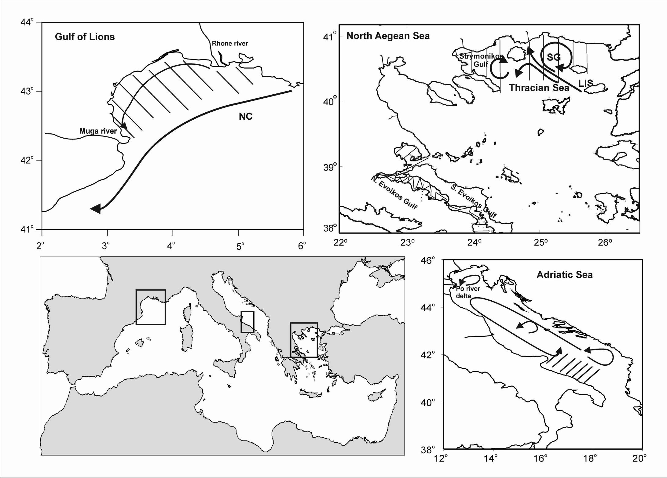
The study areas

The Gulf of Lions (Fig. 1) is one of the most productive zones in the western

Mediterranean Sea owing to a number of hydrographic features like the existence of

wide continental shelf, river run-off and strong vertical mixing during winter.

Occasional coastal upwelling is generated by local wind systems and complex

orographic effects (Millot, 1990; Lloret et al., 2001; Forget and Andre, 2007).

The North Aegean Sea is characterized by high hydrological complexity

mostly related to the Black Sea waters (BSW) that enter the Aegean Sea through the

Dardanelles strait as a surface current, the Limnos-Imvros stream (LIS) (Zervakis and

Georgopoulos, 2002, Fig. 1b). The outflow of BSW enhances local productivity and

its advection in the Aegean Sea induces high hydrological and biological complexity

(Isari et al., 2006; Somarakis and Nikolioudakis, 2007). This is further enhanced by

the presence of a series of large rivers that outflow into semi-closed gulfs (Isari et al.,

2006).

5

The Adriatic Sea is an elongated basin located in the Central Mediterranean.

Its northern section is very shallow, gently sloping, with an average bottom depth of

about 35 m and a large number of rivers discharging into it. The main outflow input

derives from the Po River in the northern part, causing large nutrient concentrations

along the coast. In contrast, the eastern coastal waters present moderate production.

The general circulation is cyclonic with a northwest flow along the eastern coast (East

Adriatic Current) and a return southeast flow (West Adriatic Current) along the

western coast (Artegiani et al., 1997a, Artegiani et al., 1997b).

MATERIALS AND METHODS

Acoustic Sampling

Acoustic data from standard monitoring stock assessment surveys were used to model

the presence of sardine juveniles during the summer in the Gulf of Lions, the North

Aegean Sea and the south western part of the Adriatic Sea. Acoustic sampling was

performed by means of scientific split-beam echosounders (Simrad EK500 and

Biosonic DT-X depending on the survey) operating at 38 kHz and calibrated

following standard techniques (Foote et al., 1987). Data were recorded at a constant

speed of 8-10 nmi h-1. Minimum sampling depth varied between 10 to 20 m

depending on the area. The size of the Elementary Distance Sampling Unit (EDSU)

was one nautical mile (nmi, 1.852 km). Midwater pelagic trawl sampling was used to

identify sardine juvenile echo traces. Sardine specimens smaller than 125 mm were

considered as juveniles as this approximates the length of first maturity for the

European sardine in the Mediterranean (Somarakis et al., 2006; Ganias et al., 2007).

Sardine juvenile echo discrimination was based on the characteristic echogram shape

6

of the schools and the catch composition of pelagic trawling that was held in the study

area (Simmonds and MacLennan, 2005). Acoustic data analysis was done with

Myriax Echoview software in the N. Aegean Sea and the Adriatic, whereas Movies+

software was used in the Gulf of Lions. Further details on acoustic sampling per study

area are described below.

In the Gulf of Lions, data were collected on board the R/V “L’EUROPE”

during July 2003-2008 (Fig. 1a). Acoustic surveys were carried out along

predetermined parallel transects, perpendicular to bathymetry with 12 nmi inter

transect distance. Records of each EDSU were combined following the method

outlined in Petitgas et al. (2003) in order to allocate fractions of the total energy

recorded (NASC: nautical area scattering coefficient) in term of biomass to the

various species captured in the trawl. For each EDSU, this biomass was reallocated in

terms of number of individuals per size and age according to the mean weight

observed in the reference trawl. In the N. Aegean Sea, acoustic data were collected on

board the R/V “PHILIA” during June 2004-2006 and 2008 along predetermined

parallel transects with 10 nmi inter-transect distance in open areas, whereas zigzag

transects were sampled inside gulfs (Fig. 1). Details of the surveys, sampling

methodology and data collected are described elsewhere (Giannoulaki et al., 2008).

Moreover, acoustic data were collected during July 2007 and 2008 in a lesser part of

North Aegean Sea, within the framework of acoustic surveys targeted for sardine

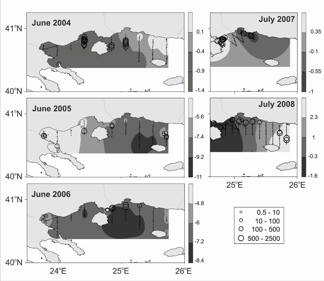
juveniles (Fig. 1b). Sardine juvenile abundance and distribution based on these

acoustic estimates shows a large degree of interannual variability in both the Gulf of

Lions and N. Aegean Sea study areas (Figs. 2, 3). However, the highest abundances

and main concentrations were located in the inner, north western part of the Gulf of

Lions and the north part of the Thracian Sea.

7

Complementary data from one acoustic survey, held in the southwest part of

the Adriatic Sea, were used to evaluate the estimated models. Data were collected on

board the R/V “DALLAPORTA” during July 2008 along predetermined parallel

transects perpendicular to the coastline with 10 nmi inter-transect distance and 8 nmi

where the continental shelf is narrow (Fig. 1d; Leonori et al., 2009; Leonori et al.,

2010).

Environmental data

Satellite environmental data as well as bathymetry data were used for modelling the

habitat of sardine juveniles in respect to environmental conditions. The Mediterranean

Sea is an area well monitored in terms of monthly satellite imagery (summarised in

Table 1). Specifically, the sea surface temperature distribution (SST in oC), the sea

surface chlorophyll concentration (CHLA in mg m-³), the Photosynthetically Active

Radiation (PAR in Einstein m-2 day-1, 1 Einstein (Ein) = 1 mole of photons), the sea

surface salinity distribution (SSS in psu based on the BCC GODAS model, Behringer

and Xue, 2004) and the sea level anomaly (SLA in cm) were downloaded from

respective databases (see Table 1) and used. These environmental variables are

considered important either as a direct influence on the distribution of sardine

juveniles (e.g. SST, CHLA) or as a proxy for causal factors (Bellido et al., 2001). For

example, SLA varies with ocean processes such as gyres, meanders and eddies

(Larnicol et al., 2002; Pujol and Larnicol, 2005) which enhance productivity and often

function as physical barriers differentiating the distribution of species or species life

stages. Similarly, satellite measured SeawiFs PAR is the photosynthetically available

radiant energy (integrated over the spectral range 400–700 nm) reaching the sea

surface over a 24 hour period (Frouin et al. 2003). It is indicative of the solar energy

8

available for photosynthesis, controlling the growth of phytoplankton thus critical also

for fisheries and carbon dynamics. It is often used to determine the euphotic depth in

the ocean taking into account light attenuation and absorption (Kirk 1996).

Bathymetry, as an indirect factor, was derived from a blending of depth soundings

collected from ships with detailed gravity anomaly information obtained from the

Geosat and ERS-1 satellite altimetry missions (Smith and Sandwell, 1997). Such

topographic variables have the potential to summarize important surrogate predictor

variables that are not captured by the available satellite variables. All monthly-

averaged satellite images from daily measurements were processed as regular grids

under a GIS (Geographic Information Systems) environment using ArcInfo GRID

software (ESRI, 1994). Thus, mean environmental monthly values for June and July

of each respective year were assigned to each survey point based on a spatial

resolution of 1.5 km (Valavanis et al., 2008).

Data analysis

Model estimation

Generalized Additive Models (GAMs) were applied in order to define the set of the

environmental factors that describe sardine juvenile distribution grounds in the N.

Aegean Sea during June and in the Gulf of Lions during July. The main advantage of

GAMs over traditional regression methods is their capability to model non-linearities

using non-parametric smoothers (Hastie and Tibshirani, 1990; Wood, 2006). The

selection of the GAMs smoothing predictors followed the method proposed by Wood

and Augustin (2002), using the ‘MGCV’ library in the R statistical software (R

Development Core Team, 2008). Each model fit was analysed in regard to the level of

deviance explained (0–100%; the higher the percentage, the more deviance

9

explained), the Akaike’s Information Criterion (AIC, the lower the better) and the

confidence region for the fit (which should not include zero throughout the range of

the predictor). The degree of smoothing was chosen based on the observed data and

the Generalized Cross Validation (GCV) method suggested by Woods (2006) and

incorporated in the ‘MGCV’ library. The GCV method is known to over-fit, therefore

the amount that the effective degree of freedom of each model counts in the GCV

score was increased by a factor γ = 1.4 (Katsanevakis et al., 2009).

Autocorrelation was evident in the spatial structure of acoustic data in both

areas. Spatial autocorrelation is known to inflate the perceived ability of models to

make realistic predictions favouring autocorrelated variables (Segurado et al., 2006),

although GAMs are not that much influenced by the effect of autocorrelation

compared to other methodologies like GLMs (Segurado et al., 2006). However, in

order to avoid this effect, we adjusted to Type I error rate by setting the accepted

significance level for each term at the more conservative value of 1%, rather than the

usual 5% (Fortin and Dale, 2005). Removing autocorrelation by means of sub-

sampling, taking into account the observed autocorrelation range as a “distance to

independence”, was not considered an option. This would be very wasteful of data

(Fortin and Dale, 2005) and may result in a non-applicable model for mapping

probabilities of habitat adequacy.

Models were constructed based on a) pooled data from both the Gulf of Lions

and N. Aegean Sea including the factorial variable of the monthly effect and based on

b) data from each area and month, separately (i.e. the Gulf of Lions in July and the N.

Aegean Sea in June). For each case, a final model was built by testing all variables

that were considered biologically meaningful, starting from a simple initial model

with one explanatory variable. The best model was selected based on the

10

minimization of the AIC score. This approach reduces the collinearity problem in the

independent variables (Sacau et al., 2005). Specifically, as response variable (y), we

used the presence/absence of sardine juveniles. As independent variables (x

covariates), we used the cube root of the bottom depth (to achieve a uniform

distribution of bottom depth), the natural logarithm of CHLA (to achieve a uniform

distribution of CHLA), SST, SSS, SLA and PAR. Original values of bottom depth

and CHLA were highly variable, thus transformation was necessary in order to

achieve uniform distributions for GAM application (Hastie and Tibshirani, 1990).

The binomial error distribution with the logit link function was used and the

natural cubic spline smoother (Hastie and Tibshirani, 1990) was applied for

independent variables smoothing and GAM fitting. Following the selection of the

main effects of the model, all first order interactions of the main effects were tested

(Wood, 2006). Validation graphs (e.g. residuals versus fitted values, QQ-plots and

residuals versus the original explanatory variables) were plotted in order to detect the

existence of any pattern and possible model misspecification. Residuals were also

checked for autocorrelation. The output of the final selected GAMs is presented as

plots of the best-fitting smooths. Interaction effects are shown as a perspective plot

without error bounds.

Model validation

In a subsequent step, each final model was tested and evaluated for its predictive

performance. For this purpose, we estimated the Receiver Operating Characteristic

curve (ROC) (Hanley and McNeil, 1982; Guisan and Zimmerman, 2000) and the

AUC metric, the area under the ROC. AUC is a threshold-independent metric, widely

used in the species’ distribution modelling literature (Franklin, 2009; Weber and

11

McClatchie, 2010). Moreover, sensitivity (i.e. the proportion of observed positives

that are correctly predicted) and specificity values (i.e. the proportion of observed

negatives that are correctly predicted) were also used for model evaluation (Lobo et

al., 2008). They were measured in relation to two threshold criteria: a) the

maximization of the specificity-sensitivity sum (MDT) and b) the prevalence values

(Jimenez-Valverde and Lobo, 2007; Lobo et al., 2008).

All metrics were also estimated for areas and periods not included in model

selection: a) both the North and South Evoikos Gulf (Aegean Sea) in June 2004 and

June 2008, b) the Gulf of Lions in July 2006 and 2007 and c) the western part of

South Adriatic Sea in July 2008. New datasets of mean monthly satellite values,

estimated for each sampled coordinate, were used for this purpose. A specific

probability of habitat adequacy for sardine juveniles was estimated for each

geographic coordinate. All metrics estimation was performed using the

“Presence/Absence” library of R statistical language.

Mapping

Based on validation results, the selected single month models were applied in a

predictive mode to provide probability estimates and habitat adequacy over a grid of

mean monthly satellite values at a GIS resolution of 4 km, the best resolution

available for satellite environmental data at a large scale, covering the entire

Mediterranean basin. Subsequently, annual habitat suitability maps were constructed

for June and July 2004 to 2008. GIS techniques were used to estimate the mean of

these annual maps, summarising the mean average probability estimates at each grid

point. Similarly, the variability map, representing the inter-annual variability in

12

nursery grounds, was also produced estimating the standard deviation of the annual

maps from 2004 to 2008.

Additionally, maps indicating areas that persistently represented juvenile

grounds within the study period were drawn. For this purpose, for each grid cell (at a

spatial resolution of 4 km) in the entire Mediterranean Sea, we calculated an Index of

Persistence (Ii), measuring the relative persistence of the cell i as an annual sardine

nursery (Fiorentino et al., 2003; Colloca et al., 2009). Let δij = 1 if the grid cell i is

included in a sardine nursery in year j, and δij = 0 if the grid cell is not included. We

computed Ii as follows:

Ii =

n

kijn 1

1 (1)

where n is the number of surveys considered. Ii ranges between 0 (cell i never

included in an annual sardine nursery area) and 1 (cell i always included in an annual

sardine nursery area) for each cell in the study area.

Preferential and occasional nursery grounds were defined following Bellier et

al. (2007) based on average, variability and persistence maps. Based on Bellier et al.

(2007) a habitat allocation map was created indicating: (a) recurrent juvenile sites -

areas with high mean, low standard deviation values and high persistence index, (b)

occasional juvenile sites - areas with high mean and high standard deviation values

(sardine juveniles are present in some years but not in others in these areas) and (c)

rare juvenile sites - areas with low mean and low standard deviation values (sardine

juveniles are rarely present in these areas). The Surfer v8.0 of the Golden Software

Inc. software was used for mapping.

Juvenile abundance versus potential habitat

13

Within the current work we also examined the relationship between the change in the

extent of “hot spot areas” (i.e., potential habitat area with high probability of sardine

juveniles presence >0.75, defined as A075) and the change in abundance of sardine

juveniles, in each study area for the study period. For this purpose in each study area

(i.e., Gulf of Lions, Adriatic Sea and North Aegean Sea, Fig. 1) we calculated the

number of grid cells presenting high probability of sardine juvenile presence (i.e., >

0.75). The abundance of sardine juveniles (i.e. annual estimates of the number of age

0 fish) was derived either from age structure stock assessment models (Cardinale et

al., 2009: N. Aegean and Adriatic Seas) and from acoustic estimates of sardine

juveniles in the case of Gulf of Lions, when no stock assessment model was available.

Abundance estimates and the extent of “hot spot areas” (i.e., extent of A075) were

both standardized and expressed, as % difference from the mean values per region in

order to assure compatibility between areas.

RESULTS

Habitat modelling

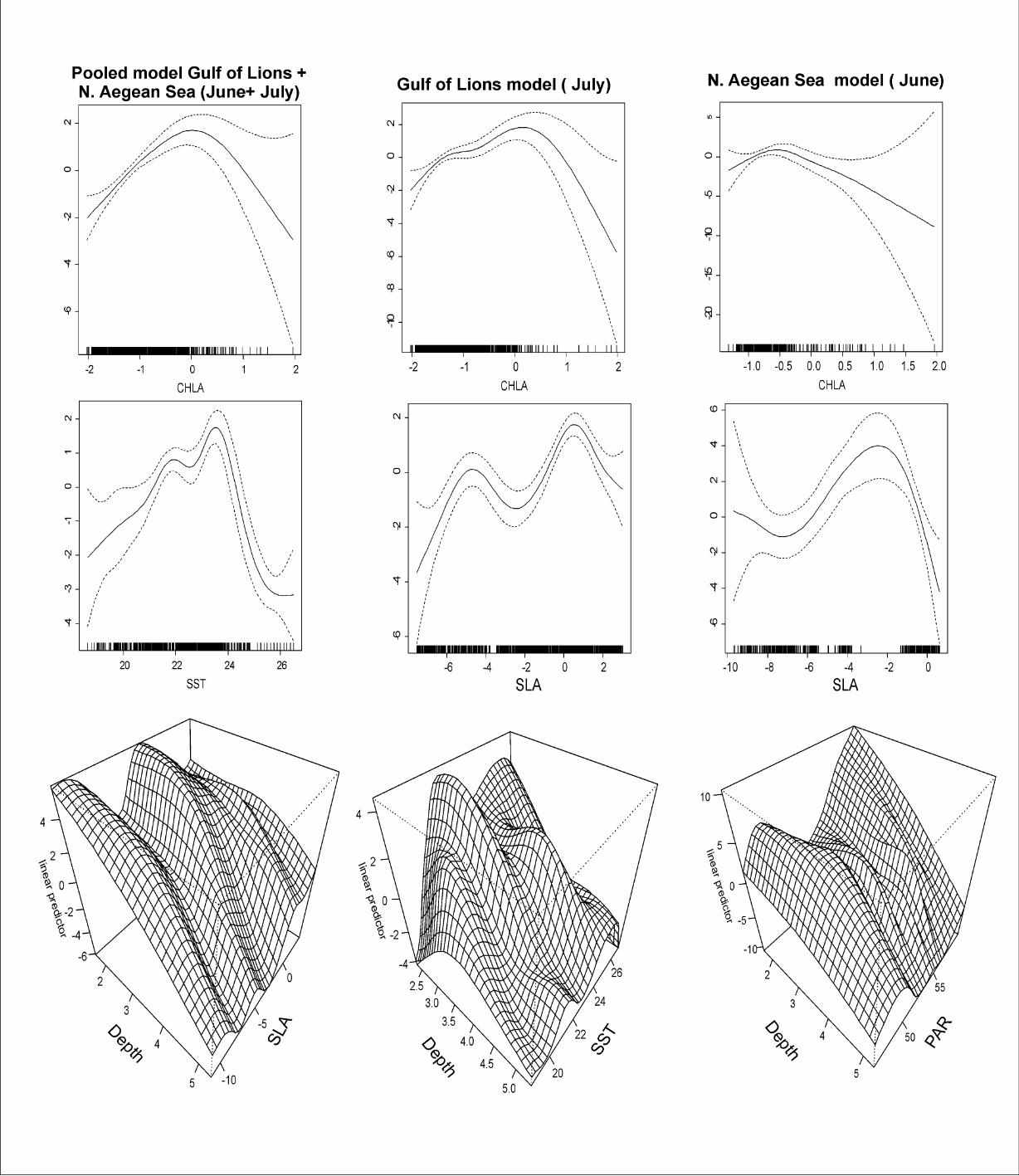
Pooled Model: Gulf of Lions and North Aegean Sea

GAMs based on the pooled data from both areas are presented on Table 2. Plots of the

best fitting smooths showed a higher probability of finding sardine juveniles present

in SST values of 21.5 - 24.5 oC, CHLA values of 0.345 - 2.718 mg m-³ (Fig. 4). The

interaction plot between Depth and SLA also indicated a higher probability of finding

sardine juveniles present in shallow waters (less than 65 m) when co-existing with

SLA values of between 0 and -5 cm (Fig. 4).

14

Gulf of Lions, July

Final selected GAM for July included as main effects: SLA, CHLA (log transformed)

and the interactive effect of Depth (cubic root transformed) and SST (Table 2). Plots

indicate a higher probability of finding sardine juveniles present in the highest

available SLA values of -1 cm to 3 cm and CHLA values of 0.345 - 2.718 mg m-³

(Fig. 4). The interaction plot between SST and Depth indicates a higher probability of

finding sardine juveniles present in the highest available values of SST (20-26 oC)

when co-existing with shallower waters (less than 60 m) (Fig. 4).

North Aegean Sea, June

The final selected GAM included as main effects: SLA, CHLA (log transformed) as

well as the interactive effect of Depth (cubic root transformed) and PAR (Table 2).

Plots indicate a higher probability of finding sardine juveniles present in SLA values

of -6 cm to 0 cm and CHLA values of 0.47-1 mg m-³. The interaction plot between

Depth and PAR indicates a higher probability of finding sardine juveniles present in

shallow waters (less than 65 m) when co-existing with PAR values of 48 to 56 Ein m-2

day-1 (Fig. 4).

In all cases, inspection of the residual plots versus fitted values and against the

original explanatory variables indicated no pattern and no apparent trend. Moreover,

residuals were checked for spatial autocorrelation by means of geostatistics (Petitgas,

2003). Results either indicate no signs of spatial autocorrelation (i.e. pure random

component) or very low levels of spatial autocorrelation (> 86% random component).

Models validation

15

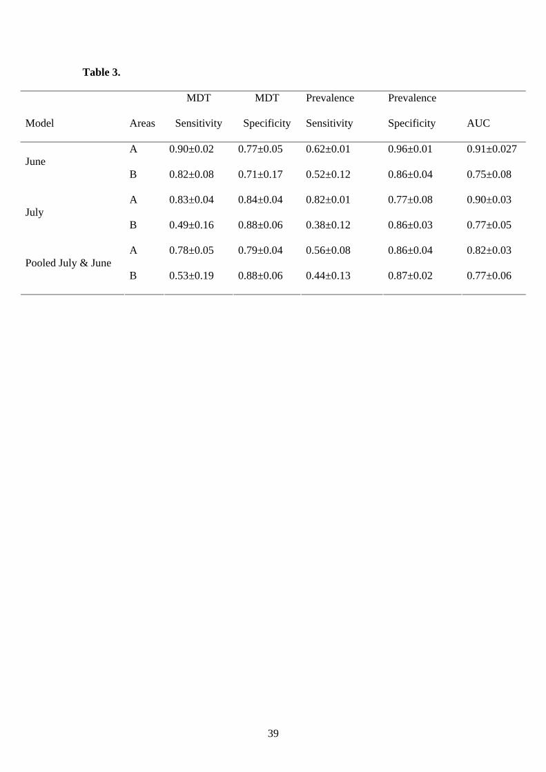
AUC generally showed good discrimination ability for all models since it exceeded on

average 0.73 for the cases that were not included in model selection (Table 3). The

lowest prediction ability was observed for areas which presented a low percentage of

sardine juvenile presence and very patchy spatial distribution of fish. Estimated

specificity and sensitivity values based on MDT and prevalence values also indicated

good discrimination ability for all models. Specificity values were generally higher

than sensitivity ones, ranging from 0.77 to 0.96 thus indicating low omission error for

all models (Table 3). Since higher sensitivity values were estimated for the single

month models, these models were selected for mapping the estimated probabilities of

habitat adequacy.

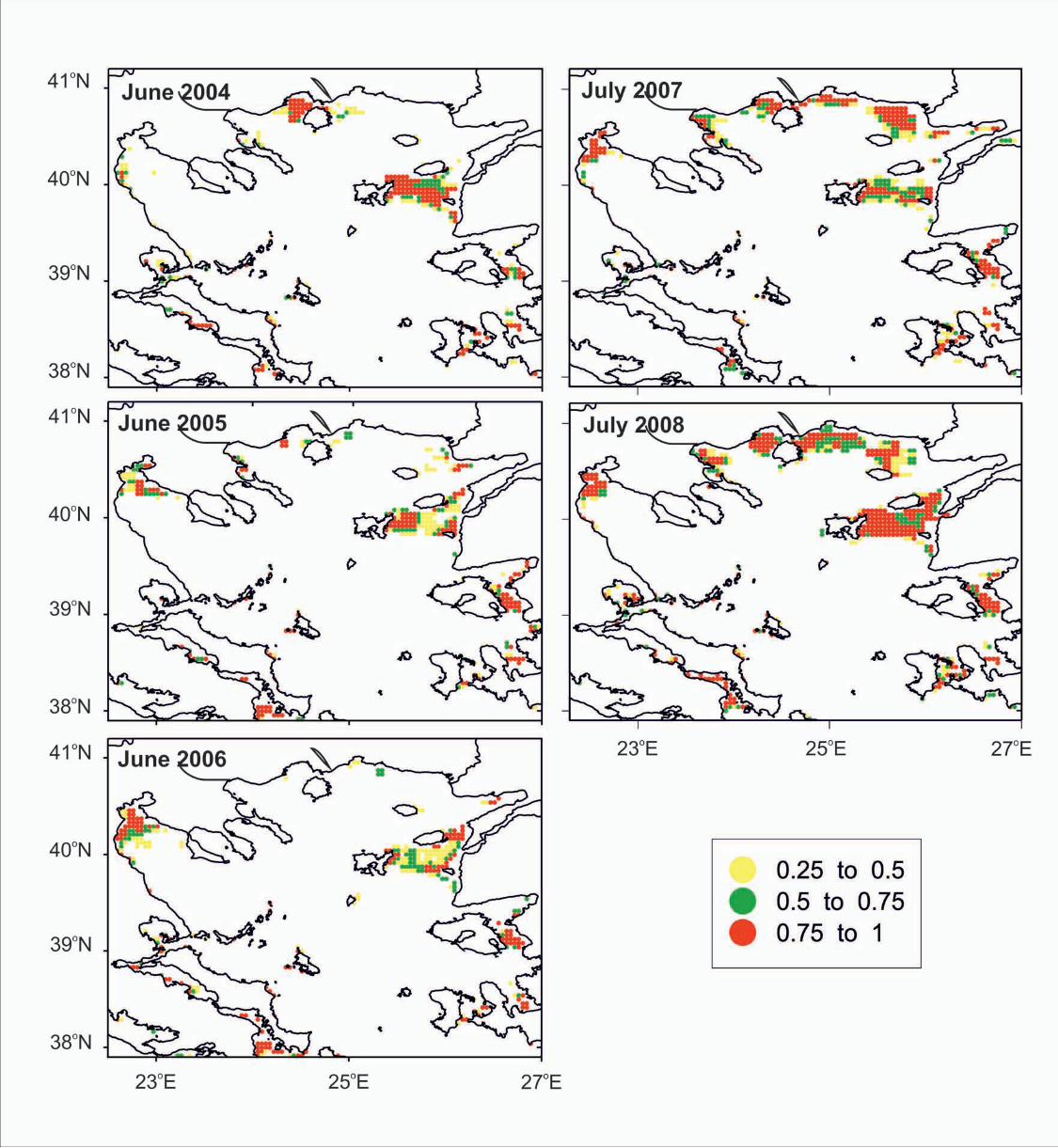
Habitat suitability maps

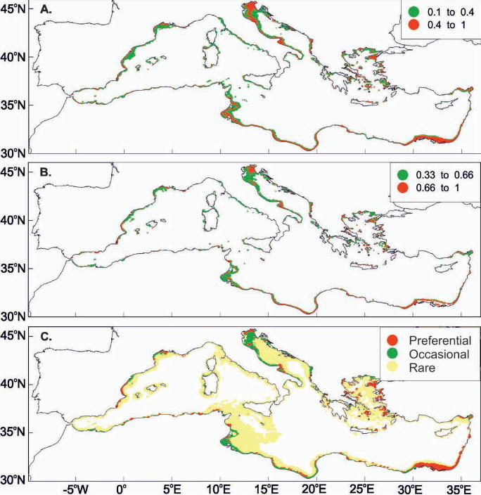
Habitat suitability maps for the study regions generally revealed an agreement

between potential nurseries and the observed distribution of sardine juveniles (Figs 2,

3 and 5, 6). The average, persistence and habitat allocation maps for the

Mediterranean within the study period (Figs 7 to 8) identified certain areas that were

consistently associated with high probability of sardine juvenile presence. In the

Western Mediterranean, these areas were located in the Adriatic Sea, the Sicily

Channel, the Tyrrhenian Sea, the Gulf of Lions, Catalan and Alboran Seas (Figs 1, 7,

8). Specifically, areas were indicated at the inner coastal waters of the Gulf of Lions,

the northern part of the Adriatic Sea, the coastal waters of the western and eastern

Adriatic, the gulfs and coastal waters of the N. Aegean Sea. Along the North Africa

coast, suitable areas were indicated in the coastal waters of Morocco, Algeria, Tunisia

and Libya (Figs 1, 7, 8). In the Eastern Mediterranean, suitable areas were revealed in

16

the Turkish coastal waters of the Aegean Sea and along the Egyptian coastline, mainly

off the Nile River Delta.

Juvenile abundance versus potential habitat

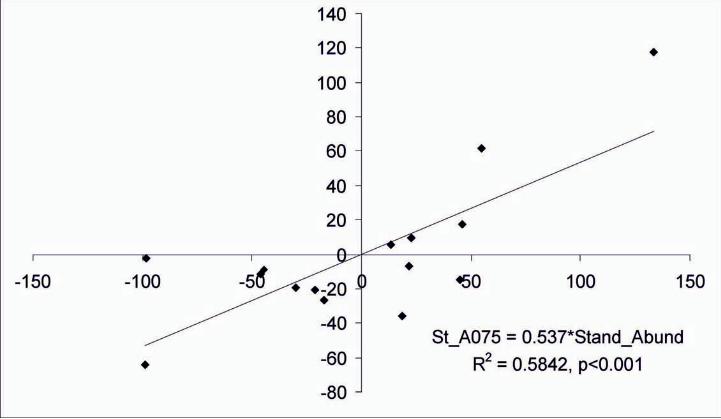
A significant positive relationship between the increase in juveniles abundance (i.e.,

standardized abundance of sardine juveniles) and the increase in habitat extent of “hot

spot areas” (i.e., standardized values of A075) was shown (Fig. 9).

DISCUSSION

Our objective was to identify and map the juvenile grounds of the European sardine in

the Mediterranean Sea during summer based on environmental associations. Data

from the western (Gulf of Lions) and the eastern part (N. Aegean Sea) of the basin

were used for this purpose.

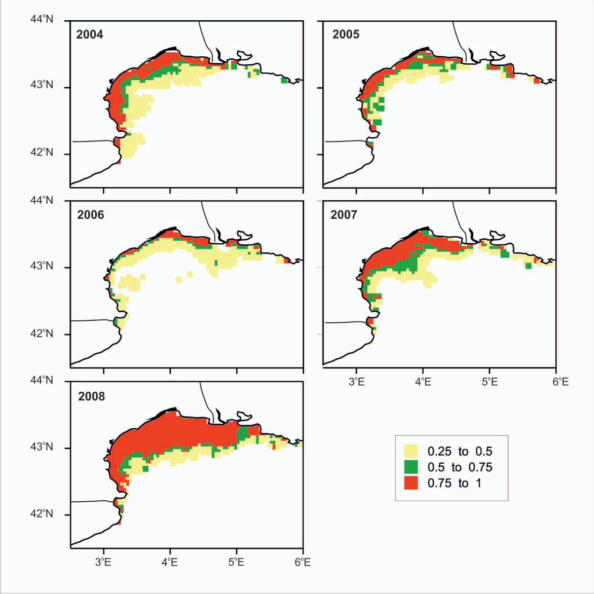
In the study areas, the visual inspection of habitat adequacy maps indicated

temporal and spatial variability in terms of suitable sites. Most persistent suitable

locations were indicated in the inner, north western part of the Gulf of Lions as well

as in the inner parts of the gulfs of the N. Aegean Sea, where shallow, warm and

productive waters exist (Figs 5, 6). In the northwestern part of the Gulf of Lions, the

presence of two large rivers, the Rhone and the Muga Rivers (Fig. 1), together with an

existing upwelling along the coast (Forget and Andre, 2007) results in a local increase

of productivity.

In the N. Aegean Sea, the more consistent nursery locations were identified at the

coastal areas of the gulfs (i.e., Thermaikos Gulf, Strymonikos Gulf and North Evoikos

Gulf) and the inner part of Thracian Sea-these areas are also under strong river

influence. Also consistent was the area between the islands, subjected to the inflow of

17

the Limnos-Imvros Stream (LIS) that carries nutrient rich Black Sea Water into

Thracian Sea (Figs. 1, 6). This further enhances productivity through the generation of

gyres and fronts (Zervakis and Georgopoulos, 2002; Somarakis et al., 2002). The

indicated areas generally agree with the results of a preliminary study on sardine

nurseries in Aegean Sea based on trawl catches (Tsagarakis et al., 2008). These

findings also agree with the general argument that pelagic fish nurseries are located in

areas of favourable food concentrations where oceanographic factors combine

favourably within an optimal environmental window (Cury and Roy, 1989; Guisande

et al., 2004; Fréon et al., 2005).

Towards a larger scale perspective, selected models were used to construct annual

maps indicating the probability of habitat adequacy for sardine juvenile presence

throughout the entire Mediterranean basin. The temporal variability of suitable

nursery areas was addressed through the estimation of the mean and the variability

map for June and July within the study period. Locations presenting high variability

as sardine nurseries were the coastal waters of the North Alboran Sea, the Sicily

Strait, the western part of the Italian Peninsula (i.e. the Ligurian and the Tyrrhenian

Sea and the area around the island of Sardinia), the Cretan Shelf in Greek seas and

areas along the coastline of the Levantine (Figs 1, 7, 8). These areas seem to represent

suitable positions for sardine juveniles occasionally, largely depending on the annual

variability of environmental conditions.

On the other hand, certain locations were quite persistent. In the north part of the

basin, besides the study regions, the most invariable nursery areas were located in the

coastal waters of the north western part of the Adriatic and around the coastal waters

of the mid-Dalmatian islands in the eastern part (Figs. 1, 7, 8). These areas coincide

with known sardine distribution grounds in the Adriatic based on acoustic surveys

18

(Ticina et al., 2005; Leonori et al., 2007a, b) as well as fishery information. The

bianchetto (fry) fishery is an old established fishery, targeting anchovy and sardine

juveniles in the south western part of the Adriatic (Morello & Arneri, 2009 and

references therein). In Spanish waters, persistent nursery areas are located in the

Catalan Sea as well as near the mouth of the Ebro River (Figs. 1, 7, 8). These areas

coincide with known distribution grounds of sardine juveniles (Giraldez et al., 2005;

Alemany et al., 2006). Similarly, in the south part of the basin along the North

African coast where information on small pelagic nursery grounds is generally

lacking, persistent areas are indicated in the coastal waters of Morocco and Algeria,

the gulf of Gabes in Tunisia and the Nile Delta area (Figs. 1, 7, 8). These areas match

the distribution grounds of sardine, as landings information from local fisheries

confirm (El-Haweet, 2001; Ben Abdallah and Gaamour 2005; Ramzi et al., 2006).

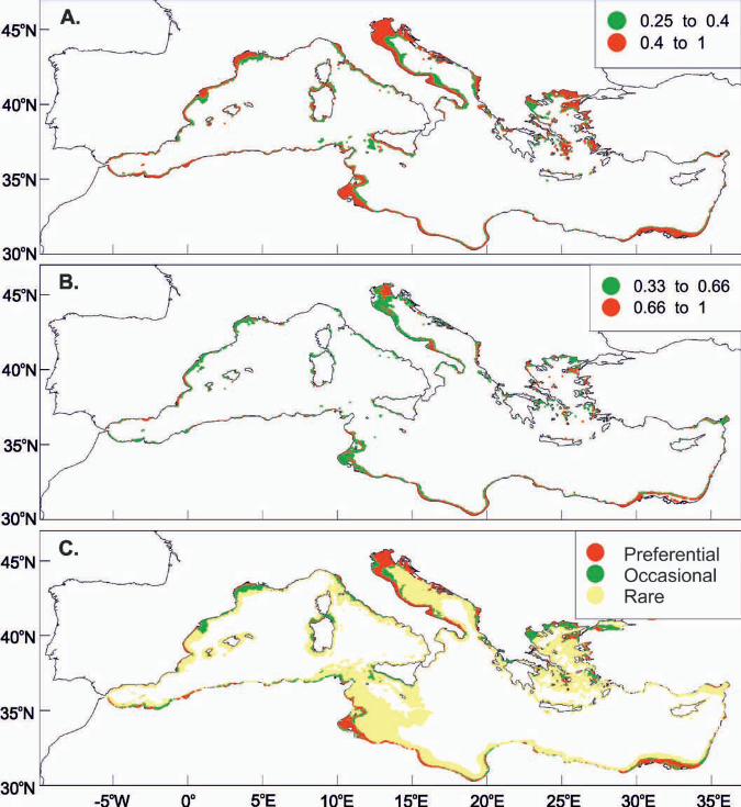
Differences in the persistent/recurrent locations between June and July were mainly

identified in the Western Mediterranean, the Strait of Sicily as well as the Levantine.

In the Western Mediterranean and the Strait of Sicily, suitable areas were more

extended in July compared to June, whereas the opposite was observed in the

Levantine (Figs. 1, 7, 8).

Areas indicated as potential juvenile grounds seem to largely match sardine adult

grounds during summer (Tugores et al., 2010), although juvenile grounds appear less

extended and more persistent in terms of locations. This is more clearly evident when

it comes to the “hot spot” areas, i.e., areas representing more than 75% probability of

suitable conditions. Spatial overlap is observed also between juvenile grounds during

summer compared to sardine spawning grounds during December (Tugores et al.,

2010).

19

Additionally, the visual inspection of sardine and anchovy juvenile grounds

(Giannoulaki et al., 2010) also shows a large degree of overlap. This most likely

reflects the peculiarities of the Mediterranean, where suitable areas favouring the

growth of juveniles, the feeding of adults and spawning processes, tend to be

localised. They are mostly associated with the existence of point sources of nutrients

that enhance productivity locally like river runoffs or local upwelling. The existence

of such limited, suitable areas along with complex oceanographic and topographic

characteristics (i.e. irregularities in the coastline and the bathymetry) are likely to

prevent long migrations for sardine between spawning, feeding and juvenile grounds.

Current work shows that in the Mediterranean, similar to large upwelling

ecosystems and the Northeast Atlantic, the juvenile grounds of sardine are mainly

situated in inshore, coastal waters (Barange et al., 1999; Checkley et al., 2009 and

references therein). However, in the high productivity ecosystems, extended

migrations of juveniles, feeding and spawning adults are observed between offshore

and inshore waters (Checkley et al., 2009 and references therein). This is not the case

in the Mediterranean where habitat maps indicate only small scale movements

between spawning, juvenile and adult grounds, are always limited to up to 100 m

depth (current findings, Tugores et al., 2010).

Our data for the N. Aegean Sea, the Adriatic Sea and the Gulf of Lions supported

the existence of density dependent effects in the populations of sardine juveniles. An

increase in the spatial extent of suitable areas was associated with an increase in the

abundance of sardine juveniles. Additional years and data availability from more

areas are required in order to further examine this relationship. However assessment

reports from different parts of the Mediterranean further support this relationship

between the extent of sardine distribution grounds and the annual variation of species

20

abundance (Bellido et al., 2008; Bigot 2009; Giannoulaki et al., 2009; Leonori et al.,

2009, 2010). In the Gulf of Lions, acoustic abundance estimates were highest in 2005,

followed by a sharp decrease in 2006 up to 2010 (Bigot and Roos, 2010). In the N.

Aegean Sea the highest abundance of sardine was found in 2003, followed by a sharp

decrease in 2004 (Giannoulaki et al., 2009). In both areas the stock fluctuations

coincided with an expansion of the distribution area in years of high abundance (Bigot

and Roos, 2010; Giannoulaki et al., 2008; 2009).

In the western Adriatic Sea, sardine distribution grounds were limited in the north

part of the basin when population levels were low in 2005, expanding towards the

central and the south part of the basin when abundance was higher in 2007 and 2008

(Leonori et al., 2009, 2010). Moreover, in the Spanish waters the high abundance of

sardine adults in 2003 to 2005 was followed by a sharp decrease in 2006 up to 2008, a

period presenting pronounced contraction of the distribution area (Bellido et al., 2008;

Cardinale et al., 2010)

In various upwelling areas, such as South Africa, Japan, California and Peru, the

sardine is known to present density dependent effects with the distribution area

increasing following an increase in population size (Barange et al., 1999; 2009). Year-

to-year variations in the year-class strength of pelagic fishes in upwelling areas are

known to be governed by upwelling intensity, whereas density-dependent processes

are particularly likely to come into play after favourable environmental conditions

have promoted the high year-class strength (Cole and McGlade, 1998). A well

established relationship between habitat extent and fish abundance in the

Mediterranean could be used to propose a spatial ecosystem indicator that could flag

situations where contraction of the potential suitable habitat implies a subsequent

decrease in the population.

21

Our approach could be a simple way to compare habitat suitability for different

species and visualise any possible spatial shifts under the effect of climate warming.

These sort of spatial shifts are reflected in the shrinkage and the expansion of suitable

areas for species. Habitat modelling results like the work presented here can provide

essential information in order to identify priority areas for the management of sardine

stocks in the Mediterranean. Large-scale conservation planning requires the

identification of priority areas or areas of particular concern such as fish nursery

grounds. Most Mediterranean fish stocks are being reported as fully exploited or

overexploited (Cardinale et al., 2010), which indicates the need for large-scale

fisheries management. The selection of priority areas for protecting juveniles and

maintaining good population status can increase the effectiveness of large-scale

fisheries management. At the same time, incorporating such habitat suitability maps

into spatial dynamic models like Ecospace (Pauly et al., 2000) can result into an

effective, highly dynamic management tool.

Acknowledgements

This study was supported and financed by the Commission of the European Union

through the Project ‘‘SARDONE: Improving assessment and management of small

pelagic species in the Mediterranean’’ (FP6 – 44294). We also want to thank the

captain and the crew of the RV ‘‘PHILIA’’, RV “L EUROPE” and RV

“DALLAPORTA” as well as all the scientists on board for their assistance during the

surveys. We also thank Dr. Alberto Santojanni for the provision of the sardine

juveniles abundance based on results of assessment model as well as Beatrice Roel

and Pierre Fréon for their constructive comments during the project.

22

REFERENCES

Alemany, F., Alvarez, I., Garcia, A., Cortes, D., Ramirez, T., Quintanilla, J., lvarez,

F.A., and Rodriguez, J.M. (2006) Postflexion larvae and juvenile daily growth

patterns of the Alboran Sea sardine (Sardina pilchardus Walb.): influence of

wind. Sci. Mar. 70: 93–104.

Artegiani, A., Bregant, D., Paschini, E., Pinardi, N., Raicich, F., and Russo A. (1997a)

The Adriatic Sea general circulation. Part I. Air-sea interactions and water mass

structure. J. Phys. Oceanogr. 27: 1492– 1514.

Artegiani, A., Bregant, D., Paschini, E., Pinardi, N., Raicich, F., and Russo, A.

(1997b) The Adriatic Sea general circulation. Part II: Baroclinic Circulation

Structure. J. Phys. Oceanogr. 27: 1515– 1532.

Barange, M., Hampton, I., and Roel, B.A. (1999) Trends in the abundance and

distribution of anchovy and sardine on the South African continental shelf in the

1990s. S. Afr. J. mar. Sci. 21: 367–391.

Barange, M., Coetzee, J., Takasuka, A., Hill, K., Gutierrez, M., Oozeki, Y., Carl van

der Lingen, C., and Agostini, V. (2009) Habitat expansion and contraction in

anchovy and sardine populations. Prog. Oceanogr. 83: 251–260.

Behringer, D.W., and Xue, Y. (2004) Evaluation of the global ocean data assimilation

system at NCEP: The Pacific Ocean. Eighth Symposium on Integrated Observing

and Assimilation Systems for Atmosphere, Oceans, and Land Surface. American

Meteorological Society 84th Annual Meeting Proceedings, Washington State

Convention and Trade Center, Washington: Seattle, pp. 11-15.

Bellido, J.M., Pierce, G., and Wang, J. (2001) Modelling intra-annual variation in

abundance of squid Loligo forbesi in Scottish waters using generalised additive

models. Fish. Res. 52: 23-39.

23

Bellido, J.M., Brown, A.M., Valavanis, V.D., Giráldez, A., Pierce, G.J., Iglesias, M.,

and Palialexis, A. (2008) Identifying Essential Fish Habitat for small pelagic

species in Spanish Mediterranean waters. Hydrobiologia 612: 171-184.

Bellier, E., Planque, B., and Petitgas, P. (2007) Historical fluctuations of spawning

area of anchovy (Engraulis encrasicolus) and sardine (Sardina pilchardus) in the

Bay of Biscay from 1967 to 2004. Fish. Oceanogr. 16(suppl. 1): 1–15.

Ben Abdallah, L., and Gaamour, A. (2005) Répartition geographique et estimation de

la biomasse des petits pélagiques des cotes tunisiennes. MedSudMed Tec. Doc. 5:

28–38.

Bigot, J.L. (2009) Stock Assessment form of Sardina pilchardus in the Gulf of Lions

(GSA07). Working paper, GFCM, SCSA, Working Group on the Small Pelagic.

General fisheries commission for the Mediterranean scientific advisory

committee, Sub-Committee for Stock Assessment, Working Group on Small

Pelagic Species, Ancona, 25-30 October 2009.

Bigot, J.L. and Roos D. (2010) Stock Assessment form of Sardina pilchardus in the

Gulf of Lions (GSA07). Working paper, GFCM, SCSA, Working Group on the

Small Pelagic. General fisheries commission for the Mediterranean scientific

advisory committee, Sub-Committee for Stock Assessment, Working Group on

Small Pelagic Species, Mazzara del Vallo, (Sicily), 1-6 November 2010.

Cardinale, M., Cheilari, A., and Ratz, H.J. (2009) Report of the SGMED-09-02

Working Group on the Mediterranean Part I. Scientific, Technical and Economic

Committee for Fisheries (STECF), 8-10 June 2009, Villasimius, Sardinia, Italy.

Cardinale, M., Cheilari, A., and Ratz, H.J. (2010) Report of the SGMED-09-02

Working Group on the Mediterranean Part I. Scientific, Technical and Economic

Committee for Fisheries (STECF), 4-8 June 2010, Iraklion, Crete, Greece.

24

Checkley, D.M., Ayon, P., Baumgartner, T.R., Bernal, M., Coetzee, J.C., Emmett, R.,

Guevara-Carrasco, R., Hutchings, L., Ibaibarriaga, L., Nakata, H., Oozeki, Y.,

Planque, B., Schweigert, J., Stratoudakis Y., and van der Lingen C.D. (2009)

Habitats. In: Climate Change and Small Pelagic Fish. A. Checkley, J. Alheit, Y.

Oozeki, and C. Roy (eds) New York: Cambridge University Press, 372 pp.

Cole, J., and McGlade, J. (1998) Clupeid population variability, the environment and

satellite imagery in coastal upwelling systems. Rev. Fish. Biol. Fish. 8: 445–471.

Colloca, F., Bartolino, V., Lasinio, J.J., Maiorano, L., Sartor, P., and Ardizzone, G.

(2009) Identifying fish nurseries using density and persistence measures. Mar.

Ecol. Progr. Ser. 381: 287-296.

Cury, P., and Roy, C. (1989) Optimal environmental window and pelagic fish

recruitment success in upwelling areas. Can. J. Fish. Aquat. Sci. 46: 670–680.

El Haweet, A., (2001) Catch composition and management of daytime purse seine

fishery on the Southern Mediterranean Sea Coast, Abu Qir Bay, Egypt. Medit.

Mar. Sci. 2(suppl. 2): 119-126.

ESRI (1994) ARC Macro Language. Environmental Systems Research Institute Inc,

USA: Redlands, CA, pp. 3-37.

Fiorentino, F., Garofalo, G, De Santi, A., Bono, G., Giusto, G.B., and Norrito, G.

(2003) Spatio-temporal distribution of recruits (0 group) of Merluccius merluccius

and Phycis blennoides (Pisces, Gadiformes) in the Strait of Sicily (Central

Mediterranean). Hydrobiologia 503: 223–236.

Foote, K.G., Knudsen, H.P., Vestenes, G., Maclennan, D.N. and Simmonds, E.J.

(1987) Calibration of acoustic instruments for fish density enstimation. A pratical

guide. ICES Coop. Res. Rep., 144, 57 pp.

25

Forget, P., and André, G. (2007) Can satellite-derived chlorophyll imagery be used to

trace surface dynamics in coastal zone? A case study in the northwestern

Mediterranean Sea. Sensors 7: 884-904.

Fortin, M.J., and Dale, M. (2005) Spatial analysis: A guide for ecologists. Cambridge

University Press.

Francis, M.P., Morrison, M.A., Leathwick, J., Walsh, C., and Middleton, C. (2005)

Predictive models of small fish presence and abundance in northern New Zealand

harbours. Est. Coast. Sh. Sci. 64: 419-435.

Franklin, J. (2009) Mapping Species Distributions. Spatial Inference and Prediction.

New York: Cambridge University Press, 320pp.

Fréon, P., Drapeau, L., David, J.H.M., Fernandez Moreno, A., Leslie, R.W.,

Oosthuizen, W.H., Shannon, L.J., and van der Lingen, C.D. (2005) Spatialized

ecosystem indicators in the southern Benguela. ICES J. Mar. Sci. 62: 459-468.

Frouin, R., Franz, B.A., Werdell, P.J., 2003. The SeaWiFS PAR product. In:

Algorithm Updates for the Fourth SeaWiFS Data Reprocessing. Hooker, S.B.,

Firestone, E.R. (eds), NASA/TM-2003-206892, 22: 46–50.

Ganias, K., Somarakis,·S., Koutsikopoulos, C., and Machias, A. (2007) Factors

affecting the spawning period of sardine in two highly oligotrophic Seas. Mar.

Biol. 151: 1559–1569.

Giannoulaki, M., Machias, A., Valavanis, V., Somarakis, S., Palialexis, A.,

Tsagarakis, K., and Papaconstantinou, C. (2007) Spatial modeling of the European

sardine habitat in the Eastern Mediterranean basin using GAMs and GIS tools.

Proceedings of the 38th CIESM Congress, April 2007, Turkey: Istanbul, pp. 486.

Giannoulaki, M., Valavanis, V.D., Palialexis, A., Tsagarakis, K., Machias, A.,

Somarakis, S., and Papaconstantinou, C. (2008) Modelling the presence of

26

anchovy Engraulis encrasicolus in the Aegean Sea during early summer, based on

satellite environmental data. Hydrobiologia 612: 225-240.

Giannoulaki, M., Somarakis, S., Machias, A., Kalianiotis, A., and Papaconstantinou,

C. (2009) Stock assessment of anchovy and sardine in GSA 22 (2000-2006)

applying Integrated Catch at Age analysis. General fisheries commission for the

Mediterranean scientific advisory committee, Sub-Committee for Stock

Assessment, Working Group on Small Pelagic Species, Ancona, 25-30 October

2009.

Giannoulaki, M., Iglesias, M., Tugores Ferra, P., Bonnano, A., Quinci, E., De Felice,

A., Gramolini, R., Liorzou, B., Tičina, V., Pyrounaki, M.M., Tsagarakis, K.,

Machias, A., Somarakis, S., Schismenou, E., Basilone, W., Leonori, I., Patti, B.,

Miguel, J., Oñate, D., Roos, D., Bigot, J.L., and Valavanis V. (2010) Identifying

the potential habitat of anchovy Engraulis encrasicolus during different life stages

in the Mediterranean Sea. ICES C.M. 2010/R:10

Giráldez, A., Torres, P., Quintanilla, L., and Baro, J. (2005) Anchovy (Engraulis

encrasicolus) and sardine (Sardina pilchardus) Stock Assessment in the GFCM

Geographical Sub-Area 01 (Northern Alboran Sea) and 06 (Northern

Spain).Working Document, GFCM, SCSA, Working Group on Small Pelagic.

Guisan, A., and Zimmermann, N.E. (2000) Predictive habitat distribution models in

ecology. Ecol. Model. 135: 147–186.

Guisande, C., Vergara, A.R., Riveiro, I., and Cabanas, J.M. (2004) Climate change

and abundance of the Atlantic-Iberian sardine (Sardina pilchardus). Fish.

Oceanogr. 13(Suppl. 2): 91-101.

Hanley, J.A., and McNeil, B.J. (1982) The meaning and use of the area under a

Receiver Operating Characteristic (ROC) curve. Radiology 143: 29-36.

27

Hastie, T., and Tibshirani, R. (1990) Generalized Additive Models. London: Chapman

and Hall, 335pp.

Hilborn, R., and Mangel, M. (1997) The Ecological Detective. Confronting Models

with data. Monographs in Populations Biology 28, Princeton: Princeton

University Press, 315pp.

Isari, S., Ramfos, A., Somarakis, S., Koutsikopoulos, C., Kallianiotis, A., and

Fragopoulou, N. (2006) Mesozooplankton distribution in relation to hydrology of

the Northeastern Aegean Sea, Eastern Mediterranean. J. Plankton Res. 28: 241–

255.

Jiménez-Valverde, A., and Lobo, J.M. (2006) The ghost of unbalanced species

distribution data in geographical model predictions. Diversity Distrib. 12: 521–

524.

Jiménez-Valverde, A., Lobo, J.M., and Hortal, J. (2008) Not as good as they seem: the

importance of concepts in species distribution modelling. Diversity Distrib.

14(suppl. 6): 885-890.

Katsanevakis, S., Maravelias, C.D., Damalas, D., Karageorgis, A.P, Tsitsika, E.V.,

Anagnostou C., and Papaconstantinou C. (2009) Spatiotemporal distribution and

habitat use of commercial demersal species in the eastern Mediterranean Sea.

Fish. Oceanogr. 18(Suppl. 6): 439-457.

Kirk, J.T.O., (1996) Light and photosynthesis in aquatic ecosystems. New York:

Cambridge University Press, 509 pp.

Larnicol, G., Ayoub, N., and Le Traon, P.Y. (2002) Major changes in Mediterranean

Sea level variability from 7 years of TOPEX/Poseidon and ERS-1/2 data. J. Mar.

Syst. 33: 63-89.

28

Lejeusne, C., Chevaldonne, P., Pergent-Martini, C., Boudouresque, C.F., and Perez,

T. (2010) Climate change effects on a miniature ocean: the highly diverse, highly

impacted Mediterranean Sea. Tr. Ecol. Evol. 25(Suppl. 4): 250-260.

Leonori, I., Azzali, M., and De Felice, A. (2007a) Assessment of small pelagic fish by

acoustic methods in south western Adriatic Sea. Working Document, GFCM

SCSA, Working Group on the Small Pelagic, Athens 13–14 September 2007.

Leonori, I., Azzali, M., and De Felice, A. (2007b) Assessment of small pelagic fish by

acoustic methods in north western Adriatic Sea. Working Document, GFCM

SCSA, Working Group on the Small Pelagic, Athens 13–14 September 2007.

Leonori, I., Azzali, M., De Felice, A., Parmiggiani, F., Marini, M., Grilli, F., and

Gramolini, R. (2009) Small pelagic fish biomass in relation to environmental

parameters in the Adriatic Sea. Proceedings of the Joint AIOL-SItE Meeting, 17-

20 September 2007, Ancona. Available online at: http://www.ecologia.it/

congressi/XVII/articles/, 213-217

Leonori, I., De Felice, A., Campanella, F. and Biagiotti, I. (2010) Stock Assessment

form of Sardina pilchardus in the Southern Adriatic Sea (GSA18). Working

paper, GFCM, SCSA, Working Group on the Small Pelagic. General fisheries

commission for the Mediterranean scientific advisory committee, Sub-Committee

for Stock Assessment, Working Group on Small Pelagic Species, Mazara del

Vallo, (Italy), 1– 6 November 2010

Lloret, J., Lleonart, J., Solea, I., and Fromentin, J.M. (2001) Fluctuations of landings

and environmental conditions in the north-western Mediterranean Sea. Fish.

Oceanogr. 10(Suppl. 1): 33-50.

29

Lobo, J.M., Jimenez-Valverde, A., and Real, R. (2008) AUC: a misleading measure of

the performance of predictive distribution models. Global Ecol. Biogeogr.

17(Suppl. 2): 145-151.

Millot, C. (1990) The Gulf of Lions' hydrodynamics. Cont. Shelf Res. 10(Suppl. 9-

11): 885-894.

Morello, E.B., and Arneri, E. (2009) Anchovy and sardine in the Adriatic Sea – An

Ecological Review. Oceanogr. Mar. Biol. Annu. Rev. 47:209-256.

Pauly, D., Christensen, V., and Walters, C. (2000) Ecopath, Ecosim, and Ecospace as

tools for evaluating ecosystem impact of fisheries. ICES J. mar. Sci. 57: 697-706.

Petitgas, P., Massé, J., Beillois, P., Lebarbier, E., and Le Cann, A. (2003) Sampling

variance of species identification in fisheries-acoustic surveys based on automated

procedures associating acoustic images and trawl hauls. ICES J. Mar. Sci. 60:

437-445.

Planque, B., Bellier, E., and Lazure, P. (2007) Modelling potential spawning habitat

of sardine (Sardina pilchardus) and anchovy (Engraulis encrasicolus) in the Bay

of Biscay. Fish. Oceanogr. 16: 16-30.

Pujol, M.I., and Larnicol, G. (2005) Mediterranean Sea eddy kinetic energy variability

from 11 years of altimetric data. J. Mar. Syst. 58: 121-142.

R Development Core Team (2008) R: A language and environment for statistical

computing. R Foundation for Statistical Computing, Vienna. Available online at:

www.R-project.org

Ramzi, A., Hbid, My.,L., and Ettahiri, O. (2006) Larval dynamics and recruitment

modelling of the Moroccan Atlantic coast sardine (Sardina pilchardus). Ecol.

Model. 197: 296–302.

30

Sacau, M., Pierce, G.J., Wang, J., Arkhipkin, A.I., Portela, J., Brickle, P., Santos,

M.B., Zuur, A.F., and Cardoso, X. (2005) The spatio-temporal pattern of

Argentine shortfin squid Illex argentinus abundance in the southwest Atlantic. Aq.

Living Res. 18: 361-372.

Segurado, P., Araújo, M.B., and Kunin, W.E. (2006) Consequences of spatial

autocorrelation for niche-based models. J. Appl. Ecol. 43(suppl. 3): 433-444.

Simmonds, J., and MacLennan, D. (2005) Fisheries acoustics, theory and practice.

2nd ed. Oxford: Blackwell Publishing, 437pp.

Smith, W.H.F., and Sandwell, D.T. (1997) Global sea floor topography from satellite

altimetry and ship depth soundings. Science 277: 1956-1962.

Somarakis, S., Drakopoulos, P., and Filippou, V. (2002) Distribution and abundance

of larval fishes in the northern Aegean Sea-eastern Mediterranean- in relation to

early summer oceanographic conditions. J. Plankton Res. 24: 339-357.

Somarakis, S., Tsianis, D.E., Machias, A., and Stergiou, K.I. (2006) An overview of

biological data related to anchovy and sardine stocks in Greek waters. In: Fishes

in Databases and Ecosystems. M.L.D. Palomares, K.I. Stergiou and D. Pauly

(eds) Fisheries Centre, University of British Columbia: Fisheries Centre Research

Reports 14, pp. 56–64.

Somarakis, S., and Nikolioudakis, N. (2007) Oceanographic habitat, growth and

mortality of larval anchovy (Engraulis encrasicolus) in the northern Aegean Sea

(eastern Mediterranean). Mar. Biol. 152: 1143–1158.

Ticina, V., Katavic, I., Dadic, V., Crubisic, L., Franicevic, M., and Ticina, V.E.

(2005) Acoustic estimates of small pelagic fish stocks in the eastern part of the

Adriatic Sea: September 2004. Working Document to GFCM, SCSA, Working

Group on the Small Pelagic, Rome 26–30 September 2005.

31

Tsagarakis, K., Machias, A., Somarakis, S, Giannoulaki, M., Palialexis, A., and

Valavanis, V.D. (2008) Habitat discrimination of juvenile sardines in the Aegean

Sea using remotely sensed environmental data. Hydrobiologia 612: 215-223.

Tugores Ferra, P., Giannoulaki, M., Iglesias, M., Bonnano, A., Tičina, V., Tsagarakis,

K., Machias, A., Patti, B., Leonori, I., De Felice, A., Campanella, F., Díaz, N.,

Giraldez, A., Valavanis, V., and Papaconstantinou, C. (2010) Habitat suitability

modeling for sardine in a highly diverse ecosystem: the Mediterranean Sea. ICES

CM: R9, ICES Annual Conference, Nantes, September 2010, France.

Valavanis, V.D., Pierce, G.J., Zuur, A.F., Palialexis, A., Saveliev, A., Katara, I., and

Wang, J. (2008) Modelling of Essential Fish Habitat based on Remote Sensing,

Spatial Analysis and GIS. Hydrobiologia 612(suppl. 1): 5-20.

Weber, E.D., and McClatchie, S. (2010) Predictive models of northern anchovy

Engraulis mordax and Pacific sardine Sardinops sagax spawning habitat in the

California Current. Mar. Ecol. Prog. Ser. 406: 251-263.

Wood, S.N., and Augustin, N.H. (2002) GAMs with integrated model selection using

penalized regression splines and applications to environmental modelling. Ecol.

Model. 157: 157–177.

Wood, S.N. (2006) Generalized Additive Models. An Introduction with R. London:

Chapman & Hall, 392pp.

Zervakis, V., and Georgopoulos, D. (2002) Hydrology and circulation in the Northern

Aegean Sea throughout 1997 and 1998. Medit. Mar. Sci. 3: 5-19.

32

Tables headings

Table 1. Environmental satellite parameters and their characteristics. Measurements

are extracted from the respective databases on a daily scale and in a next step

averaged on a monthly basis.

Table 2. Final GAM models selected. Analysis of deviance for GAM covariates and

their interactions of the final model fitted. Level of significance was set to 0.05. June

data refer to North Aegean Sea, July data refer to Gulf of Lions. The (:) sign denotes

interaction. Res. d.f= residual degrees of freedom; Res. Deviance=residual deviance;

AIC=Akaike Information Criterion value; P-value (chi-square)= significance values.

SST: Sea Surface Temperature, CHLA: chlorophyll concentration (log transformed),

Depth: Bathymetry (cubic root transformed), SLA: Sea Level Anomaly, PAR:

Photosynthetic Active Radiation.

Table 3. Mean values of sensitivity and specificity accuracy measures ± standard

error (sterr) for two threshold criteria: MDT (maximize the specificity-sensitivity

sum) and prevalence values. The estimated area under the ROC curve (AUC) for each

model is also indicated. A: Areas and years included in model selection, B: areas and

years not included in model selection.

33

Figures legends

Fig. 1. Map of the study areas where transects of acoustic sampling are shown. Map

of water circulation is also shown. Arrows indicate the presence of fronts and gyres

(redrawn from Millot, 1990; Somarakis et al., 2002; Artegiani 1997a). LIS: Limnos–

Imvos Steam, NC; Northern Current, Positions and names of the main rivers in the

area are also shown. Toponyms mentioned in the text are also indicated.

Fig 2. Abundance (in Biomass in tonnes/nm2) of sardine juveniles in the Gulf of Lions

during July 2003, 2004, 2005 and 2008. Sea Level Anomaly distribution (in cm) per

respective study year is also shown.

Fig 3. Echo abundance index Nautical Area Scattering Coefficient (NASC in m2/nm2)

of sardine juveniles in the N. Aegean Sea during June 2004, 2005, 2006, July 2007

and 2008. Sea Level Anomaly distribution (in cm) per respective study year is also

shown.

Fig. 4. Coefficients of the Generalized Additive Models (GAMs) for sardine juveniles

against environmental variables for each selected model. CHLA: log transformed

Surface chlorophyll concentration (in mg m-³) SST: Sea Surface Temperature (oC),

SLA: Sea Level Anomaly (in cm), Depth: Cube root transformed Bottom Depth (in

m), PAR: Photosynthetically Active Radiation (in Einstein m-2 day-1). The interaction

plots are also shown. Black thick lines indicate the value of GAMs coefficient, dotted

lines represent the confidence intervals at p = 0.05. The rug under the single variable

effects plots indicates the density of points for different variable values.

34

Fig 5. Annual habitat suitability maps indicating the probability for sardine juvenile

presence in the Gulf of Lions, based on GAM model from July in the same area. GIS

resolution for mean monthly satellite values used for prediction was 4 km. Scale

indicates probability range.

Fig 6. Annual habitat suitability maps indicating the probability for sardine juvenile

presence in the N. Aegean Sea, based on GAM model from June in the same area.

GIS resolution for mean monthly satellite values used for prediction was 4 km. Scale

indicates probability range.

Fig. 7. (A) Mean probability, (B) persistence index and (C) allocation maps

concerning habitat suitability for the presence of sardine juveniles in the

Mediterranean Sea for June. GIS resolution for mean monthly satellite values used

was 4 km concerning June 2004 to 2008. Numbers indicate toponyms mentioned in

the text. 1. Alboran Sea, 2. Sicily Strait, 3. Gabes Gulf, 4. Nile Delta, 5. Levantine

basin, 6. Cretan Sea, 7. Aegean Sea, 8. Tyrrhenian Sea, 9. Island of Sardinia, 10.

Ligurian Sea, 11. Catalan Sea, 12. Gulf of Lions, 13. Adriatic Sea, 14. Dalmatian

islands.

Fig 8. (A) Mean probability, (B) persistence index and (C) allocation maps

concerning habitat suitability for the presence of sardine juveniles in the

Mediterranean Sea for July. GIS resolution for mean monthly satellite values used

was 4 km concerning July 2004 to 2008. Numbers indicate toponyms mentioned in

the text. 1. Alboran Sea, 2. Sicily Strait, 3. Gabes Gulf, 4. Nile Delta, 5. Levantine

basin, 6. Cretan Sea, 7. Aegean Sea, 8. Tyrrhenian Sea, 9. Island of Sardinia, 10.

35

36

Ligurian Sea, 11. Catalan Sea, 12. Gulf of Lions, 13. Adriatic Sea, 14. Dalmatian

islands.

Fig. 9. Graph presents the relationship between the standardized sardine juveniles

abundance and the standardized extent of “hot spot areas” (i.e., potential habitat area

A075) concerning the Gulf of Lions, Adriatic Sea and N. Aegean Sea. Standardized

Abundance: Abundance estimates of sardine juveniles expressed as % difference from

the mean values per region, Standardized A075: extent of area A075 expressed as %

difference from the mean values per region.

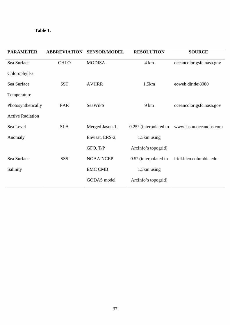
Table 1.

PARAMETER ABBREVIATION SENSOR/MODEL RESOLUTION SOURCE

Sea Surface

Chlorophyll-a

CHLO MODISA 4 km oceancolor.gsfc.nasa.gov

Sea Surface

Temperature

SST AVHRR 1.5km eoweb.dlr.de:8080

Photosynthetically

Active Radiation

PAR SeaWiFS 9 km oceancolor.gsfc.nasa.gov

Sea Level

Anomaly

SLA Merged Jason-1,

Envisat, ERS-2,

GFO, T/P

0.25° (interpolated to

1.5km using

ArcInfo’s topogrid)

www.jason.oceanobs.com

Sea Surface

Salinity

SSS NOAA NCEP

EMC CMB

GODAS model

0.5° (interpolated to

1.5km using

ArcInfo’s topogrid)

iridl.ldeo.columbia.edu

37

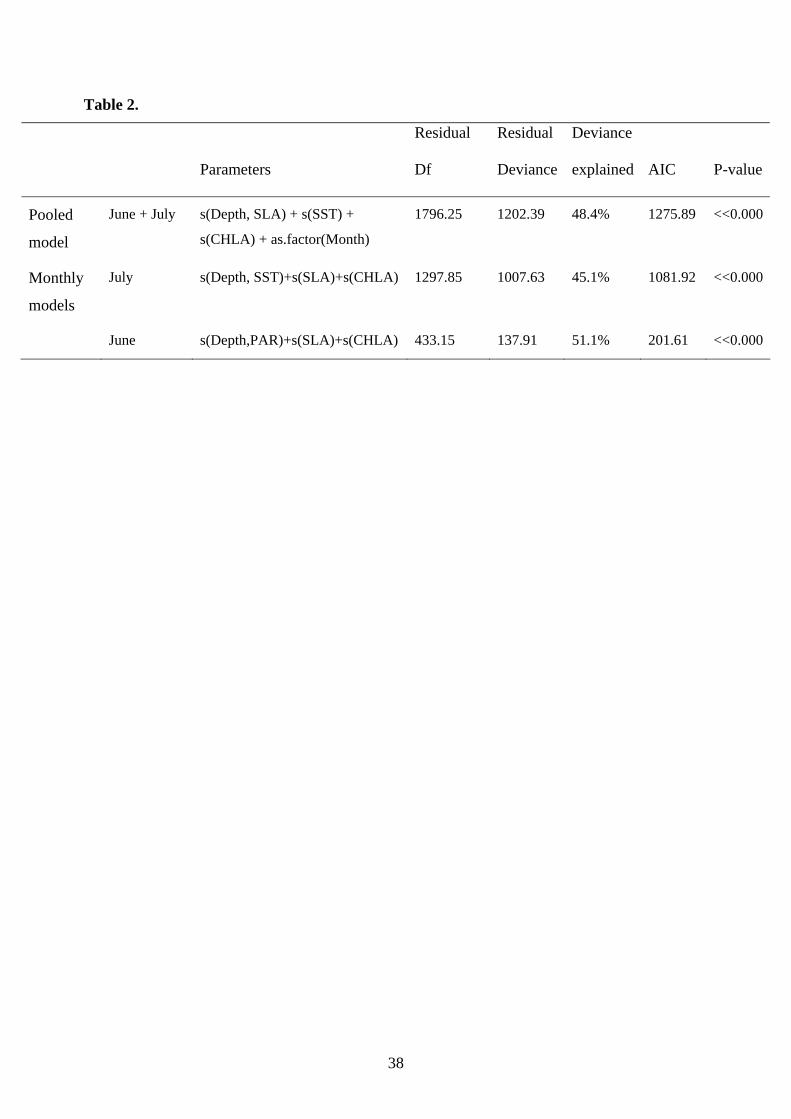
Table 2.

Parameters

Residual

Df

Residual

Deviance

Deviance

explained AIC P-value

Pooled

model

June + July s(Depth, SLA) + s(SST) +

s(CHLA) + as.factor(Month)

1796.25 1202.39 48.4% 1275.89 <<0.000

Monthly

models

July s(Depth, SST)+s(SLA)+s(CHLA) 1297.85 1007.63 45.1% 1081.92 <<0.000

June s(Depth,PAR)+s(SLA)+s(CHLA) 433.15 137.91 51.1% 201.61 <<0.000

38

39

Table 3.

Model Areas

MDT

Sensitivity

MDT

Specificity

Prevalence

Sensitivity

Prevalence

Specificity AUC

A 0.90±0.02 0.77±0.05 0.62±0.01 0.96±0.01 0.91±0.027 June

B 0.82±0.08 0.71±0.17 0.52±0.12 0.86±0.04 0.75±0.08

A 0.83±0.04 0.84±0.04 0.82±0.01 0.77±0.08 0.90±0.03 July

B 0.49±0.16 0.88±0.06 0.38±0.12 0.86±0.03 0.77±0.05

A 0.78±0.05 0.79±0.04 0.56±0.08 0.86±0.04 0.82±0.03 Pooled July & June

B 0.53±0.19 0.88±0.06 0.44±0.13 0.87±0.02 0.77±0.06