half-car model based lqr control of active...
TRANSCRIPT

Fan 1
Half-Car Model Based LQR Control of
Active Suspension
Xingchen Fan
ME 131 Final Project
Professor Hedrick
Spring 2013
1. INTRODUCTION
Suspension is one of the key connections between road and vehicle body. It not only
supports the static weight of the vehicle, but also influences the comfort of passengers, the
road holding abilities of tires and vehicle’s handling characters. Several criteria are usually
adopted to evaluate the performance of suspension, namely ride quality, suspension
deflection (also called rattle space) and tire deflection. For passive suspension, when damping
and stiffness are tuned to improve one performance, the other two are likely to be penalized.
The inevitable tradeoffs in passive suspension design motivate the implementation of active
suspensions, in which a controlled actuator is able to provide force in addition to that from
conventional spring/damper unit. Since the evaluation of suspension performance consists of
several criteria, it is reasonable to weight each criterion and put them in a performance index.
Linear quadratic regulator (LQR) is a good choice for such optimization based control. LQR
control has already been successfully implemented on quarter-car model (Rajamai). This
Fan 2
paper is dedicated to see how LQR control works on a more complicated half-car model with
pitch movement. Therefore, in addition to vertical acceleration, angular acceleration about
center of gravity (CG) is also used to assess ride quality. In fact, the half-car model based
LQR controller for active suspension also works for roll control; however, this paper only
focuses on pitch control.
2. HALF-CAR MODEL
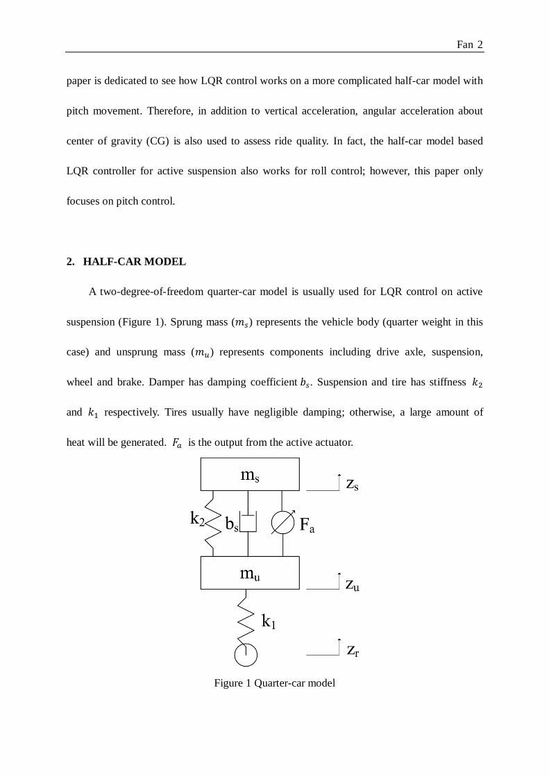
A two-degree-of-freedom quarter-car model is usually used for LQR control on active
suspension (Figure 1). Sprung mass (𝑚𝑠) represents the vehicle body (quarter weight in this
case) and unsprung mass (𝑚𝑢) represents components including drive axle, suspension,
wheel and brake. Damper has damping coefficient 𝑏𝑠. Suspension and tire has stiffness 𝑘2
and 𝑘1 respectively. Tires usually have negligible damping; otherwise, a large amount of
heat will be generated. 𝐹𝑎 is the output from the active actuator.
Figure 1 Quarter-car model

Fan 3
In our analysis, we consider the most common conditions where wheels are always in
contact with ground. Thus, all displacements are measured from the static equilibrium
position, allowing gravity to be neglected.
The half-car model combines two quarter-car models with a shared sprung mass, where
a human model could be attached. The model has four degrees of freedom: sprung mass’s
vertical translation, its rotation about center of gravity, front and rear unsprung masses’
vertical translations. By adopting the same assumptions in quarter-car model, the
gravitational effect is neglected.
Figure 2 Half-car model
The equations of motion for half-car model are shown in Appendix I. Notice the positive
pitch is defined when the vehicle body rotates clockwise, or the front end of the vehicle
moves down.

Fan 4
With four degrees of freedom and their first time-derivatives, an eight-state linear
time-invariant (LTI) system is developed to represent the plant. The state-space representation
of half-car model is shown below:
�̇� = 𝐴𝑥 + 𝐵𝑢 + 𝐿𝑟
𝑦 = 𝐶𝑥 + 𝐷𝑟 (1)
Matrices A, B, L, C and D are included in Appendix I. In this case, x is an 8 × 1 state vector;
u is a 2 × 1 input vector including front and rear actuator forces (𝐹𝑎𝑓 and 𝐹𝑎𝑟); r is a 2 ×
1 disturbance vector containing road inputs to front and rear tires (𝑧𝑟𝑓 and 𝑧𝑟𝑟); y is the
output vector with all criteria, which will be discussed in the next section. For road inputs, the
vehicle is assumed to travel at constant speed, so the rear tire experiences the same road input
as the front tire does, but with a constant time delay.
3. LQR CONTROL WITH VARIOUS CRITERIA
The design of the controller is associated with the criteria in which we are interested. For
suspension, we are interested in:
i. Ride quality
Passengers feel uncomfortable when they experience large vertical accelerations.
Hence the acceleration of center of gravity ( �̈�𝑐𝑔 ) is one of the criteria.
Furthermore, with only �̈�𝑐𝑔, it’s possible that CG is at constant height, while
front and rear ends of the vehicle are oscillating. Therefore, the pitch acceleration
about the center of gravity (�̈�𝑐𝑔) is also taken into account. Penalties on �̈�𝑐𝑔 and

Fan 5
�̈�𝑐𝑔 are able to reduce the acceleration of every point on sprung mass, even
though the acceleration of specific passenger point is not considered in this paper.
Moreover, people feel uncomfortable when acceleration itself is changing fast; so
the first time-derivative of acceleration, jerk (𝑧𝑐𝑔 and 𝜃𝑐𝑔), can also be used as a
criterion. However, to simplify the system, it is not included in the performance
index. Jerk data is extracted from simulation results through numerical
differentiation of �̈�𝑐𝑔 and �̈�𝑐𝑔.
ii. Suspension deflection (rattle space)
Suspension deforms under load so it can absorb some energy from the road.
Suspension deflection (𝑧𝑠𝑓 − 𝑧𝑢𝑓 and 𝑧𝑠𝑟 − 𝑧𝑢𝑟 ) refers to the change in distance
between sprung and unsprung mass. How much suspension is allowed to deflect
depends on the limited space between wheels and vehicle body. If suspension
bottoms out, there will be a rigid connection between wheels and vehicle body.
Passengers will feel really uncomfortable. Small vehicles usually have a low ride
height, so their suspensions must deflect within a smaller range. Therefore,
suspension deflection should be held under control.
iii. Tire deflection
Tires are generally stiffer than suspension but they still deflect under load. Tire
deflection (𝑧𝑢𝑓 − 𝑧𝑟𝑓 and 𝑧𝑢𝑟 − 𝑧𝑟𝑟 ) is defined as the change in distance
between unsprung mass and road. Tires’ road holding ability is sensitive to
change in normal force and the shape of the contact patch. Excessive tire

Fan 6
deflection can cause tires to lose grip and result in slipping. Thus tire deflection
has to be minimized.
iv. Actuator force
Actuators only provide limited forces (𝐹𝑎𝑓 and 𝐹𝑎𝑟). Typical hydraulic actuators
in the market today are able to supply as much as 20,000 N. In addition,
compared to passive and semi-active suspensions, higher power consumption is
one of the drawbacks of active suspension. Therefore, it is necessary to constrain
the actuator output both to save power and to ensure that the desired force is
achievable.
The resultant performance index is defined as below:
𝐽 = ∫ [𝜌0�̈�𝑐𝑔2 + 𝜌1�̈�𝑐𝑔
2+ 𝜌2(𝑧𝑠𝑓 − 𝑧𝑢𝑓)
2+ 𝜌3(𝑧𝑠𝑟 − 𝑧𝑢𝑟)2
∞
0
+ 𝜌4�̇�𝑠𝑓2 + 𝜌5�̇�𝑠𝑟
2
+𝜌6(𝑧𝑢𝑓 − 𝑧𝑟𝑓)2
+ 𝜌7(𝑧𝑢𝑟 − 𝑧𝑟𝑟)2 + 𝜌8 �̇�𝑢𝑓2 + 𝜌8�̇�𝑢𝑟
2 + 𝜌10𝐹𝑎𝑓2 + 𝜌11𝐹𝑎𝑟
2]𝑑𝑡 (2)
It is the cost function for a quadratic programming problem, which should be minimized. For
weights in the performance index, only relative values matter. Therefore, the weight for z̈cg2
is assumed to be 1 whenever this term is penalized. All other weights are referenced to it. The
performance index is rearranged to the standard form as below:
𝐽 = ∫ [∞
0𝑥𝑇𝑄𝑥 + 2𝑥𝑇𝑁𝑢 + 𝑢𝑇𝑅𝑢]𝑑𝑡 (3)
where Q, N and R are shown in Appendix II. These three matrices are large and have
complicated entries. Hence instead of putting them down in state-space representation
explicitly, they are defined elementwise in MATLAB code.
It is shown that the solution to this optimization problem is feedback control: 𝑢 = −𝐺𝑥,

Fan 7
where 𝐺 = 𝑅−1(𝐵𝑇𝑃 + 𝑁), and P is the solution to algebraic Riccati equation (Rajamani):
(𝐴 − 𝐵𝑅−1𝑁)𝑇𝑃 + 𝑃(𝐴 − 𝐵𝑅−1𝑁) + (𝑄 − 𝑁𝑇𝑅−1𝑁) − 𝑃𝐵𝑅−1𝐵𝑇𝑃 = 0 (4)
Accordingly, equation 1 becomes:
�̇� = (𝐴 − 𝐵𝐺)𝑥 + 𝐿𝑟
𝑦 = 𝐶𝑥 + 𝐷𝑟 (5)
In this case, r becomes the input to the system; y is a 6 × 1 vector containing the criteria:
y = [�̈�𝑐𝑔 �̈�𝑐𝑔 𝑧𝑠𝑓 − 𝑧𝑢𝑓𝑧𝑠𝑟 − 𝑧𝑢𝑟 𝑧𝑢𝑓 − 𝑧𝑟𝑓 𝑧𝑢𝑟 − 𝑧𝑟𝑟]𝑇 (6)
With corresponding matrices C and D, we are able to obtain transfer functions from road
inputs to each criterion. Firstly, the state-space representation is written in s-domain:
𝑠𝑋 = (𝐴 − 𝐵𝐺)𝑋 + 𝐿𝑅
𝑌 = 𝐶𝑋 + 𝐷𝑅 (7)
Then the equations are reorganized and X is cancelled out. We obtain the closed-loop transfer
function from R to Y:
𝑌
𝑅= 𝐶(𝑠𝐼 − 𝐴 + 𝐵𝐺)−1𝐿 + 𝐷 (8)
This will be used in frequency analysis of the LQR controller in the next section.
4. SIMULATION RESULTS
The half-car model based LQR controller is simulated in MATLAB. Instead of the
analytical methods introduced in the previous section, some built-in MATLAB functions are
used to significantly simplify simulation and analysis: given A, B, Q, R and N, “lqr” computes
the feedback gain matrix G, which is used in every iteration in transient analysis. One of the

Fan 8
requirements for input argument to “lqr” function is that R matrix:
𝑅 = [
1
𝑚2 + 𝜌101
𝑚2
1
𝑚2
1
𝑚2 + 𝜌11
] (9)
has to be positive definite, where 𝜌10 and 𝜌11 are from equation 2. Therefore, for “lqr” to
work, there must be some penalty on actuator force, i.e. 𝜌10 = 𝜌11 ≠ 0. Small 𝜌10 and 𝜌11
(e.g. 10−10) represent fully operating actuators, and large 𝜌10 and 𝜌11 (e.g. 10−1) make the
system behave like a passive one. In addition, given A, B, C and D, built-in function “ss2tf”
computes the corresponding transfer function, which is used in frequency analysis.
The front and rear halves of the model are assumed to be symmetrical. The vehicle
parameters used in simulation are (SI units): 𝑘𝑠𝑓 = 𝑘𝑠𝑟 = 16000, 𝑏𝑠𝑓 = 𝑏𝑠𝑟 = 1000, 𝑘𝑡𝑓 =
𝑘𝑡𝑟 = 160000, 𝑚𝑢𝑓 = 𝑚𝑢𝑟 = 45, 𝑚 = 650, 𝐼 = 2200, 𝐿 = 2.8, 𝑙𝑓 = 𝑙𝑟 = 1.4 (Rajamani).
The speed of the vehicle is assumed to be 15 m/s (54 km/h).
Simulation consists of two parts: transient analysis and frequency analysis.
I. Transient analysis
In this part of simulation, the results are shown in time domain. The road input is a
typical speed hump with a height of 20 cm and a chord length of 4 m. The front tire hits the
hump at time t = 1 s. The results for passive half-car model (u = 0) are shown below:

Fan 9
Figure 3 CG position and pitch movement for passive suspension
When the front tire hits the hump, the sprung mass lifts and rotates counterclockwise.
That’s why a positive vertical displacement and a negative pitch movement are observed in
Figure 3. As the vehicle passes the hump, the perturbations gradually die out and the vehicle
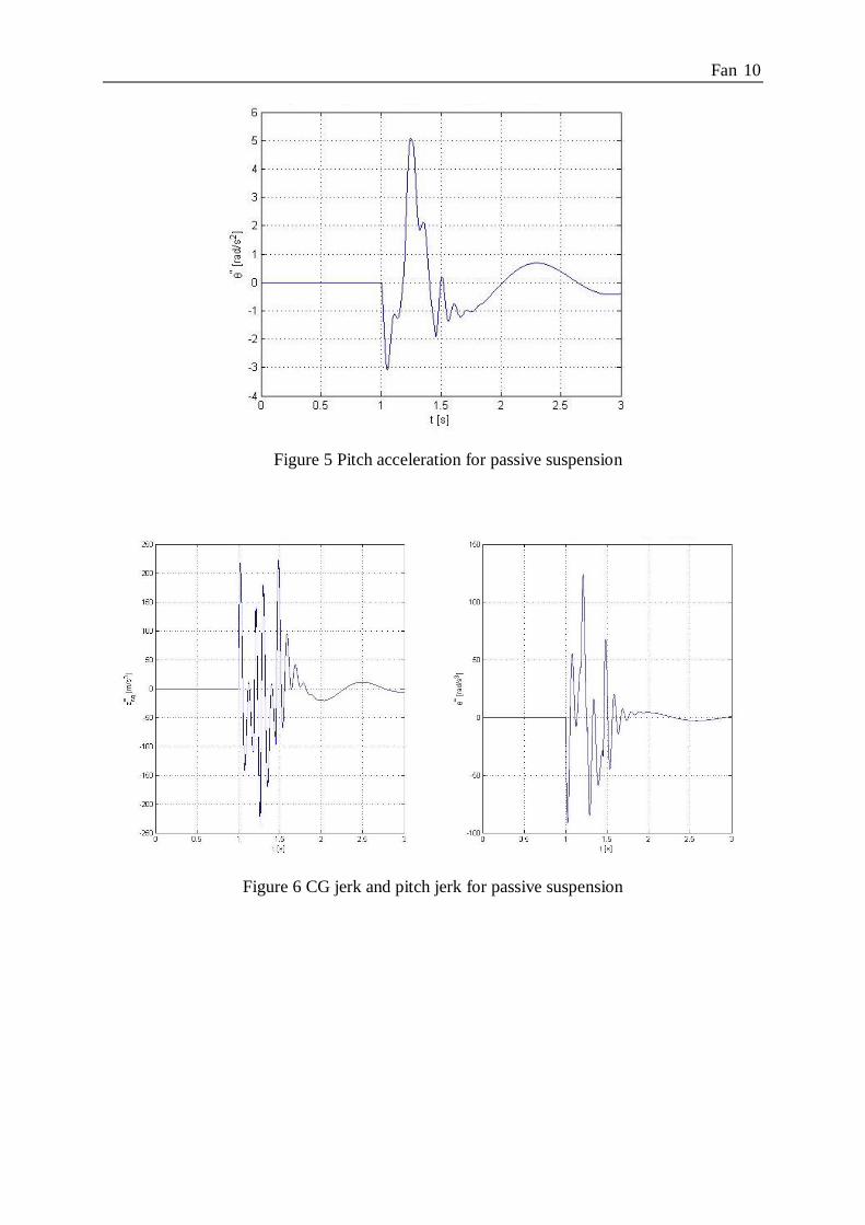
returns to its equilibrium position. This is further confirmed by Figure 4 and 5, and jerk data
in Figure 6.
Figure 4 CG acceleration for passive suspension
Fan 10
Figure 5 Pitch acceleration for passive suspension
Figure 6 CG jerk and pitch jerk for passive suspension

Fan 11
Figure 7 Front suspension deflection and tire deflection for passive suspension
Figure 8 Rear suspension deflection and tire deflection for passive suspension

Fan 12
From Figure 7 and 8, it is shown that the front suspension is first compressed and then
stretched. The rear suspension behaves similarly but with a time delay of about 0.2 s. Also,
we can see that a large portion of the displacement of the speed hump (0.2 m) is transferred to
CG and rattle space.
When a fully operating LQR controller (𝜌10 = 𝜌11 = 10−10) with penalty only on CG
acceleration is implemented, some results are shown below:
Figure 9 CG position and pitch movement for 𝜌0 = 1
It is obvious from Figure 8 that CG of sprung mass barely moves up (less than 1 mm).
There is a significant improvement in CG acceleration and jerk in Figure 10 and 11 compared
to passive ones in Figure 4 and 6. However, comparing Figure 3 and 9 shows that nothing has
improved in terms of pitch movement, suggesting that when the front and rear actuators are
working to reduce �̈�𝑐𝑔, the vehicle is still rotating about CG.

Fan 13
Figure 10 CG acceleration for 𝜌0 = 1
Figure 11 CG jerk for 𝜌0 = 1
Then we implement a fully operating LQR controller with penalty on both CG
acceleration and pitch acceleration. The results are shown below:

Fan 14
Figure 12 CG position and pitch movement for 𝜌0 = 𝜌1 = 1
Compared to the passive system in Figure 3, both vertical translation and pitch
movement have decreased considerably. The vehicle is barely moving up and down or
rotating about the CG. The CG acceleration in Figure 13 and the pitch acceleration in Figure
14 both confirm this improvement. This also suggests that every point on sprung mass has
small acceleration.
Figure 13 CG acceleration for 𝜌0 = 𝜌1 = 1

Fan 15
Figure 14 Pitch acceleration for 𝜌0 = 𝜌1 = 1
Figure 15 shows the front and rear actuators’ force outputs. Again a time delay of 0.2 s
between front and rear is obvious in the plots. The desired force is no more than 7000 N,
which is totally achievable with available actuators.
Figure 15 Front and rear actuator forces for 𝜌0 = 𝜌1 = 1
If power consumption is a concern, the weights on 𝐹𝑎𝑓 and 𝐹𝑎𝑟 can increase. The

Fan 16
performance will deteriorate though since actuators will not work as hard as they can.
Furthermore, it is clear from the plots above that it takes a long time for the system to settle
down to its equilibrium position. In Figure 15, the actuators still have small oscillating
outputs after the speed hump. This problem can be solved by penalizing the actuator outputs
more heavily. An example is shown in Figure 16 and 17:
Figure 16 CG position and pitch movement for 𝜌0 = 𝜌1 = 1 and 𝜌10 = 𝜌11 = 10−6

Fan 17
Figure 17 Front and rear actuator forces for 𝜌0 = 𝜌1 = 1 and 𝜌10 = 𝜌11 = 10−6
Overall, a half-car model based LQR controller is able to significantly improve ride
quality. However, just like passive suspension tuning, active suspension tuning has tradeoffs.
The inverse relationship between actuator force and ride quality improvement is already
discussed above. In addition, there are suspension deflection and tire deflection criteria.
When ride quality improves, those two criteria are usually sacrificed. This will be studied
through frequency analysis in the next section.
II. Frequency analysis
In this part of simulation, the results are shown in frequency domain, and mainly based
on Bode magnitude plots of transfer functions from road input to each criterion. For a typical

Fan 18
commercial vehicle, the natural frequencies for sprung mass and unsprung mass are about 1
Hz and 10 Hz. Also, humans are most sensitive to frequencies in this range. Therefore, the
frequency band at which the analysis is done is from 0.1 Hz and 100 Hz. In the following
plots, for comparison, the dashed lines illustrate the frequency response of the passive system,
while the solid lines represent the system with LQR control. Since the front and rear halves of
the vehicle has identical parameters, only the frequency response of the front suspension is
plotted. Moreover, because the CG acceleration and the pitch acceleration are often weighted
equally, they have very similar frequency responses. Only one of them will be plotted.
When the LQR controller is tuned for ride quality (𝜌0 = 𝜌1 = 1) without any penalty on
other criteria, the frequency responses of CG acceleration and pitch acceleration are shown in
Figure 18 and 19 respectively:
Figure 18 CG acceleration for 𝜌0 = 𝜌1 = 1

Fan 19
It is shown that ride quality has improved over the entire frequency band except the peak
at about 10 Hz. This is consistent with the results shown by Rajamani: acceleration transfer
function has an invariant point at ω = √𝑘𝑡
𝑚𝑢, which is approximately the natural frequency of
unsprung mass.
As ride quality improves, suspension deflection and tire deflection become worse
(Figure 20), especially at unsprung mass resonant frequency. Moreover, the suspension
deflection transfer function has an asymptote at low frequencies, which does not exist in
passive suspension. The results are consistent with those obtained from quarter-car model
(Rajamani).
Figure 19 Front suspension deflection for 𝜌0 = 𝜌1 = 1
Fan 20
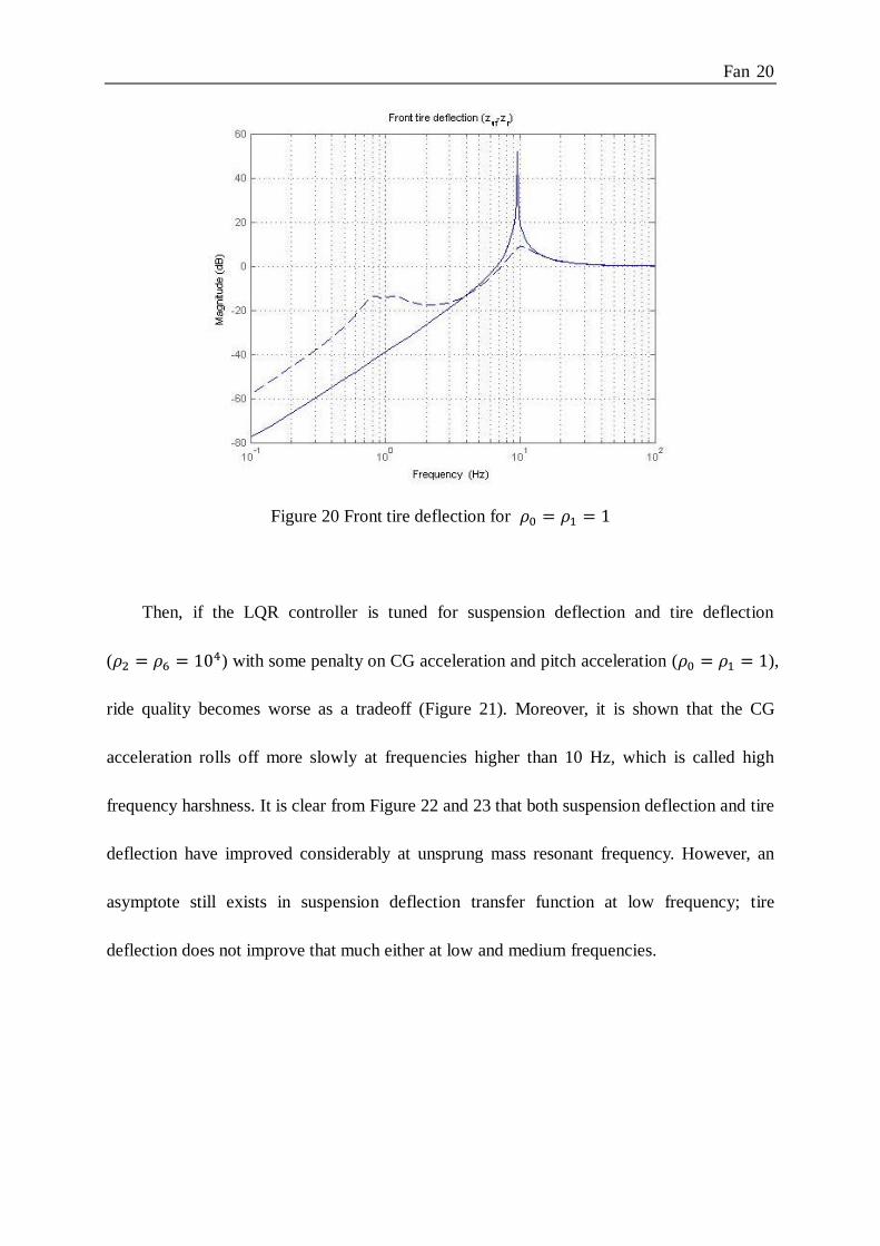
Figure 20 Front tire deflection for 𝜌0 = 𝜌1 = 1
Then, if the LQR controller is tuned for suspension deflection and tire deflection
(𝜌2 = 𝜌6 = 104) with some penalty on CG acceleration and pitch acceleration (𝜌0 = 𝜌1 = 1),
ride quality becomes worse as a tradeoff (Figure 21). Moreover, it is shown that the CG
acceleration rolls off more slowly at frequencies higher than 10 Hz, which is called high
frequency harshness. It is clear from Figure 22 and 23 that both suspension deflection and tire
deflection have improved considerably at unsprung mass resonant frequency. However, an
asymptote still exists in suspension deflection transfer function at low frequency; tire
deflection does not improve that much either at low and medium frequencies.

Fan 21
Figure 21 CG acceleration for 𝜌0 = 𝜌1 = 1, 𝜌2 = 𝜌6 = 104
Figure 22 Front suspension deflection for 𝜌0 = 𝜌1 = 1, 𝜌2 = 𝜌6 = 104

Fan 22
Figure 23 Front tire deflection for 𝜌0 = 𝜌1 = 1, 𝜌2 = 𝜌6 = 104
To sum it up, like passive suspensions, tradeoffs are inevitable in active suspension
design. A considerable amount of improvement in ride quality requires a significant sacrifice
in suspension deflection and tire deflection, and vice versa; improvement at sprung mass
frequency results in deterioration at unsprung mass frequency, and vice versa.
5. CONCLUSION
A half-car model based LQR controller gives vehicle designers more freedom in
suspension tuning. The suspension is allowed to have different setups with fixed geometry
and fixed-rate spring/damper unit. However, a balance between ride quality, suspension
deflection, tire deflection and power consumption is important.
Another thing to notice is that most results from the half-car model based LQR

Fan 23
controller are consistent with those obtained from the quarter-car model based LQR controller.
This suggests that the decoupled quarter-car model may be sufficient for all desired
improvements from active suspension. An intuition behind this is as follows. For the half-car
model, two degrees of freedom define the position of sprung mass. In this paper, the vertical
translation of center of gravity and the rotation about center of gravity are used. However,
another choice will be the vertical translations of front and rear suspension attachment points
(�̈�𝑠𝑓 and �̈�𝑠𝑟). In that case, the model is basically decoupled into two quarter-car models. In
addition, the quarter-car model is much simpler mathematically.
REFERENCES
Rajamani, Rajesh. Vehicle Dynamics and Control. NewYork: Springer, 2012. Chapter 10, 11
and 12.

APPENDIX I
Equations of motion:
Acceleration of center of gravity:
𝑚�̈�𝑐𝑔 = −𝑘𝑠𝑓(𝑧𝑠𝑓 − 𝑧𝑢𝑓) − 𝑏𝑠𝑓(�̇�𝑠𝑓 − �̇�𝑢𝑓) − 𝑘𝑠𝑟(𝑧𝑠𝑟 − 𝑧𝑢𝑟) − 𝑏𝑠𝑟(�̇�𝑠𝑟 − �̇�𝑢𝑟) + 𝐹𝑎𝑓 + 𝐹𝑎𝑟
Pitch acceleration:
𝐼�̈� = −𝑙𝑓[−𝑘𝑠𝑓(𝑧𝑠𝑓 − 𝑧𝑢𝑓) − 𝑏𝑠𝑓(�̇�𝑠𝑓 − �̇�𝑢𝑓) + 𝐹𝑎𝑓] + 𝑙𝑟[−𝑘𝑠𝑟(𝑧𝑠𝑟 − 𝑧𝑢𝑟) − 𝑏𝑠𝑟(�̇�𝑠𝑟 − �̇�𝑢𝑟) + 𝐹𝑎𝑟]
Acceleration of front unsprung mass:
𝑚𝑢𝑓�̈�𝑢𝑓 = 𝑘𝑠𝑓(𝑧𝑠𝑓 − 𝑧𝑢𝑓) + 𝑏𝑠𝑓(�̇�𝑠𝑓 − �̇�𝑢𝑓) − 𝑘𝑡𝑓(𝑧𝑢𝑓 − 𝑧𝑟𝑓) − 𝐹𝑎𝑓
Acceleration of rear unsprung mass:
𝑚𝑢𝑟�̈�𝑢𝑟 = 𝑘𝑠𝑟(𝑧𝑠𝑟 − 𝑧𝑢𝑟) + 𝑏𝑠𝑟(�̇�𝑠𝑟 − �̇�𝑢𝑟) − 𝑘𝑡𝑟(𝑧𝑢𝑟 − 𝑧𝑟𝑟) − 𝐹𝑎𝑟
Displacement of front and rear sprung mass:
𝑧𝑠𝑓 = 𝑧𝑐𝑔 − 𝑙𝑓𝜃
𝑧𝑠𝑟 = 𝑧𝑐𝑔 + 𝑙𝑟𝜃

𝐴 =
[
0 1
−𝑘𝑠𝑓 + 𝑘𝑠𝑟
𝑚−
𝑏𝑠𝑓 + 𝑏𝑠𝑟
𝑚
0 0𝑙𝑓𝑘𝑠𝑓 − 𝑙𝑟𝑘𝑠𝑟
𝑚
𝑙𝑓𝑏𝑠𝑓 − 𝑙𝑟𝑏𝑠𝑟
𝑚0 0
𝑙𝑓𝑘𝑠𝑓 − 𝑙𝑟𝑘𝑠𝑟
𝐼
𝑙𝑓𝑏𝑠𝑓 − 𝑙𝑟𝑏𝑠𝑟
𝐼
0 1
−𝑙𝑓
2𝑘𝑠𝑓 + 𝑙𝑟2𝑘𝑠𝑟
𝐼−
𝑙𝑓2𝑏𝑠𝑓 + 𝑙𝑟
2𝑏𝑠𝑟
𝐼
0 0𝑘𝑠𝑓
𝑚
𝑏𝑠𝑓
𝑚
0 0𝑘𝑠𝑟
𝑚
𝑏𝑠𝑟
𝑚0 0
−𝑙𝑓𝑘𝑠𝑓
𝐼 −
𝑙𝑓𝑏𝑠𝑓
𝐼
0 0
𝑙𝑟𝑘𝑠𝑟
𝐼
𝑙𝑟𝑏𝑠𝑟
𝐼0 0 𝑘𝑠𝑓
𝑚𝑢𝑓
𝑏𝑠𝑓
𝑚𝑢𝑓
0 0
−𝑙𝑓𝑘𝑠𝑓
𝑚𝑢𝑓 −
𝑙𝑓𝑏𝑠𝑓
𝑚𝑢𝑓
0 0 𝑘𝑠𝑟
𝑚𝑢𝑟
𝑏𝑠𝑟
𝑚𝑢𝑟
0 0𝑙𝑟𝑘𝑠𝑟
𝑚𝑢𝑟
𝑙𝑟𝑏𝑠𝑟
𝑚𝑢𝑟
0 1
−𝑘𝑠𝑓 + 𝑘𝑡𝑓
𝑚𝑢𝑓 −
𝑏𝑠𝑓
𝑚𝑢𝑓
0
0
0
0
0
0
0
0
0 1
−𝑘𝑠𝑟 + 𝑘𝑡𝑟
𝑚𝑢𝑟−
𝑏𝑠𝑟
𝑚𝑢𝑟]
𝐵 =
[
01
𝑚0
−𝑙𝑓𝐼
01
𝑚0𝑙𝑟𝐼
0
−1
𝑚𝑢𝑓
0
0
0
0
0
−1
𝑚𝑢𝑟]
, 𝐿 =
[
0000
0000
0𝑘𝑡𝑓
𝑚𝑢𝑓
0
0
0
0
0𝑘𝑡𝑟
𝑚𝑢𝑟]
1
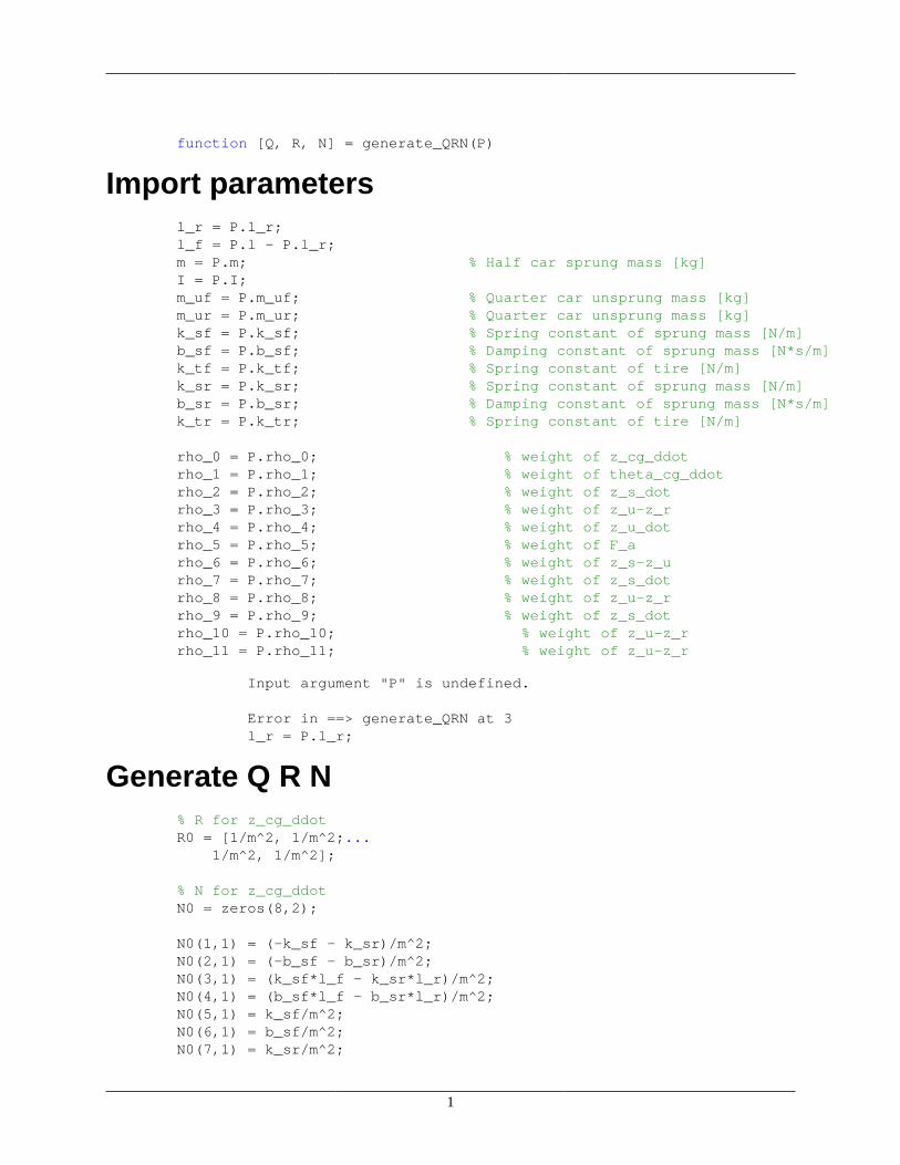
function [Q, R, N] = generate_QRN(P)
Import parametersl_r = P.l_r;l_f = P.l - P.l_r;m = P.m; % Half car sprung mass [kg]I = P.I;m_uf = P.m_uf; % Quarter car unsprung mass [kg]m_ur = P.m_ur; % Quarter car unsprung mass [kg]k_sf = P.k_sf; % Spring constant of sprung mass [N/m]b_sf = P.b_sf; % Damping constant of sprung mass [N*s/m]k_tf = P.k_tf; % Spring constant of tire [N/m]k_sr = P.k_sr; % Spring constant of sprung mass [N/m]b_sr = P.b_sr; % Damping constant of sprung mass [N*s/m]k_tr = P.k_tr; % Spring constant of tire [N/m]
rho_0 = P.rho_0; % weight of z_cg_ddotrho_1 = P.rho_1; % weight of theta_cg_ddotrho_2 = P.rho_2; % weight of z_s_dotrho_3 = P.rho_3; % weight of z_u-z_rrho_4 = P.rho_4; % weight of z_u_dotrho_5 = P.rho_5; % weight of F_arho_6 = P.rho_6; % weight of z_s-z_urho_7 = P.rho_7; % weight of z_s_dotrho_8 = P.rho_8; % weight of z_u-z_rrho_9 = P.rho_9; % weight of z_s_dotrho_10 = P.rho_10; % weight of z_u-z_rrho_11 = P.rho_11; % weight of z_u-z_r
Input argument "P" is undefined.
Error in ==> generate_QRN at 3l_r = P.l_r;
Generate Q R N% R for z_cg_ddotR0 = [1/m^2, 1/m^2;... 1/m^2, 1/m^2];
% N for z_cg_ddotN0 = zeros(8,2);
N0(1,1) = (-k_sf - k_sr)/m^2;N0(2,1) = (-b_sf - b_sr)/m^2;N0(3,1) = (k_sf*l_f - k_sr*l_r)/m^2;N0(4,1) = (b_sf*l_f - b_sr*l_r)/m^2;N0(5,1) = k_sf/m^2;N0(6,1) = b_sf/m^2;N0(7,1) = k_sr/m^2;

2
N0(8,1) = b_sr/m^2;N0(:,2) = N0(:,1);
% Q for z_cg_ddotQ0 = zeros(8,8);
Q0(1,2) = (b_sf*k_sf + b_sf*k_sr + b_sr*k_sf + b_sr*k_sr)/m^2;Q0(1,3) = (-k_sf^2*l_f + k_sr^2*l_r - k_sf*k_sr*l_f + k_sf*k_sr*l_r)/m^2;Q0(1,4) = (-b_sf*k_sf*l_f - b_sf*k_sr*l_f + b_sr*k_sf*l_r +... b_sr*k_sr*l_r)/m^2;Q0(1,5) = (-k_sf^2 - k_sf*k_sr)/m^2;Q0(1,6) = (-b_sf*k_sf - b_sf*k_sr)/m^2;Q0(1,7) = (-k_sr^2 - k_sf*k_sr)/m^2;Q0(1,8) = (-b_sr*k_sf - b_sr*k_sr)/m^2;
Q0(2,3) = (-b_sf*k_sf*l_f - b_sr*k_sf*l_f + b_sf*k_sr*l_r +... b_sr*k_sr*l_r)/m^2;Q0(2,4) = (-b_sf^2*l_f + b_sr^2*l_r - b_sf*b_sr*l_f + b_sf*b_sr*l_r)/m^2;Q0(2,5) = (-b_sf*k_sf - b_sr*k_sf)/m^2;Q0(2,6) = (-b_sf^2 - b_sf*b_sr)/m^2;Q0(2,7) = (-b_sf*k_sr - b_sr*k_sr)/m^2;Q0(2,8) = (-b_sr^2 - b_sf*b_sr)/m^2;
Q0(3,4) = (b_sf*k_sf*l_f^2 + b_sr*k_sr*l_r^2 - b_sf*k_sr*l_f*l_r -... b_sr*k_sf*l_f*l_r)/m^2;Q0(3,5) = (k_sf^2*l_f - k_sf*k_sr*l_r)/m^2;Q0(3,6) = (b_sf*k_sf*l_f - b_sf*k_sr*l_r)/m^2;Q0(3,7) = (-k_sr^2*l_r + k_sf*k_sr*l_f)/m^2;Q0(3,8) = (b_sr*k_sf*l_f - b_sr*k_sr*l_r)/m^2;
Q0(4,5) = (b_sf*k_sf*l_f - b_sr*k_sf*l_r)/m^2;Q0(4,6) = (b_sf^2*l_f - b_sf*b_sr*l_r)/m^2;Q0(4,7) = (b_sf*k_sr*l_f - b_sr*k_sr*l_r)/m^2;Q0(4,8) = (-b_sr^2*l_r + b_sf*b_sr*l_f)/m^2;
Q0(5,6) = b_sf*k_sf/m^2;Q0(5,7) = k_sf*k_sr/m^2;Q0(5,8) = b_sr*k_sf/m^2;
Q0(6,7) = b_sf*k_sr/m^2;Q0(6,8) = b_sf*b_sr/m^2;
Q0(7,8) = b_sr*k_sr/m^2;
Q0(1,1) = (k_sf^2 + k_sr^2 + 2*k_sf*k_sr)/m^2;Q0(2,2) = (b_sf^2 + b_sr^2 + 2*b_sf*b_sr)/m^2;Q0(3,3) = (k_sf^2*l_f^2 + k_sr^2*l_r^2 - 2*k_sf*k_sr*l_f*l_r)/m^2;Q0(4,4) = (b_sf^2*l_f^2 + b_sr^2*l_r^2 - 2*b_sf*b_sr*l_f*l_r)/m^2;Q0(5,5) = k_sf^2/m^2;Q0(6,6) = b_sf^2/m^2;Q0(7,7) = k_sr^2/m^2;Q0(8,8) = b_sr^2/m^2;
% R for theta_cg_ddot

3
R1 = [l_f^2/I^2, -l_f*l_r/I^2;... -l_f*l_r/I^2, l_r^2/I^2];
% N for theta_cg_ddotN1 = zeros(8,2);
N1(1,1) = (-k_sf*l_f^2 + k_sr*l_f*l_r)/I^2;N1(2,1) = (-b_sf*l_f^2 + b_sr*l_f*l_r)/I^2;N1(3,1) = (k_sf*l_f^3 + k_sr*l_f*l_r^2)/I^2;N1(4,1) = (b_sf*l_f^3 + b_sr*l_f*l_r^2)/I^2;N1(5,1) = k_sf*l_f^2/I^2;N1(6,1) = b_sf*l_f^2/I^2;N1(7,1) = -k_sr*l_f*l_r/I^2;N1(8,1) = -b_sr*l_f*l_r/I^2;N1(1,2) = (-k_sr*l_r^2 + k_sf*l_f*l_r)/I^2;N1(2,2) = (-b_sr*l_r^2 + b_sf*l_f*l_r)/I^2;N1(3,2) = (-k_sr*l_r^3 - k_sf*l_f^2*l_r)/I^2;N1(4,2) = (-b_sr*l_r^3 - b_sf*l_f^2*l_r)/I^2;N1(5,2) = -k_sf*l_f*l_r/I^2;N1(6,2) = -b_sf*l_f*l_r/I^2;N1(7,2) = k_sr*l_r^2/I^2;N1(8,2) = b_sr*l_r^2/I^2;
% Q for theta_cg_ddotQ1 = zeros(8,8);
Q1(1,2) = (b_sf*k_sf*l_f^2 + b_sr*k_sr*l_r^2 - b_sr*k_sf*l_f*l_r -... b_sf*k_sr*l_f*l_r)/I^2;Q1(1,3) = (-k_sf^2*l_f^3 + k_sr^2*l_r^3 - k_sf*k_sr*l_f*l_r^2 +... k_sf*k_sr*l_f^2*l_r)/I^2;Q1(1,4) = (-b_sf*k_sf*l_f^3 + b_sf*k_sr*l_f^2*l_r + b_sr*k_sr*l_r^3 -... b_sr*k_sf*l_f*l_r^2)/I^2;Q1(1,5) = (-k_sf^2*l_f^2 + k_sf*k_sr*l_f*l_r)/I^2;Q1(1,6) = (-b_sf*k_sf*l_f^2 + b_sf*k_sr*l_f*l_r)/I^2;Q1(1,7) = (-k_sr^2*l_r^2 + k_sf*k_sr*l_f*l_r)/I^2;Q1(1,8) = (b_sr*k_sf*l_f*l_r - b_sr*k_sr*l_r^2)/I^2;
Q1(2,3) = (-b_sf*k_sf*l_f^3 + b_sr*k_sf*l_f^2*l_r - b_sf*k_sr*l_f*l_r^2 +... b_sr*k_sr*l_r^3)/I^2;Q1(2,4) = (-b_sf^2*l_f^3 + b_sr^2*l_r^3 - b_sf*b_sr*l_f*l_r^2 +... b_sf*b_sr*l_f^2*l_r)/I^2;Q1(2,5) = (-b_sf*k_sf*l_f^2 + b_sr*k_sf*l_f*l_r)/I^2;Q1(2,6) = (-b_sf^2*l_f^2 + b_sf*b_sr*l_f*l_r)/I^2;Q1(2,7) = (b_sf*k_sr*l_f*l_r - b_sr*k_sr*l_r^2)/I^2;Q1(2,8) = (-b_sr^2*l_r^2 + b_sf*b_sr*l_f*l_r)/I^2;
Q1(3,4) = (b_sf*k_sf*l_f^4 + b_sr*k_sr*l_r^4 + b_sf*k_sr*l_f^2*l_r^2 +... b_sr*k_sf*l_f^2*l_r^2)/I^2;Q1(3,5) = (k_sf^2*l_f^3 + k_sf*k_sr*l_f*l_r^2)/I^2;Q1(3,6) = (b_sf*k_sf*l_f^3 + b_sf*k_sr*l_f*l_r^2)/I^2;Q1(3,7) = (-k_sr^2*l_r^3 - k_sf*k_sr*l_f^2*l_r)/I^2;Q1(3,8) = (-b_sr*k_sf*l_f^2*l_r - b_sr*k_sr*l_r^3)/I^2;
Q1(4,5) = (b_sf*k_sf*l_f^3 + b_sr*k_sf*l_f*l_r^2)/I^2;

4
Q1(4,6) = (b_sf^2*l_f^3 + b_sf*b_sr*l_f*l_r^2)/I^2;Q1(4,7) = (-b_sf*k_sr*l_f^2*l_r - b_sr*k_sr*l_r^3)/I^2;Q1(4,8) = (-b_sr^2*l_r^3 - b_sf*b_sr*l_f^2*l_r)/I^2;
Q1(5,6) = b_sf*k_sf*l_f^2/I^2;Q1(5,7) = -k_sf*k_sr*l_f*l_r/I^2;Q1(5,8) = -b_sr*k_sf*l_f*l_r/I^2;
Q1(6,7) = -b_sf*k_sr*l_f*l_r/I^2;Q1(6,8) = -b_sf*b_sr*l_f*l_r/I^2;
Q1(7,8) = b_sr*k_sr*l_r^2/I^2;
Q1(1,1) = (k_sf^2*l_f^2 + k_sr^2*l_r^2 - 2*k_sf*k_sr*l_f*l_r)/I^2;Q1(2,2) = (b_sf^2*l_f^2 + b_sr^2*l_r^2 - 2*b_sf*b_sr*l_f*l_r)/I^2;Q1(3,3) = (k_sf^2*l_f^4 + k_sr^2*l_r^4 + 2*k_sf*k_sr*l_f^2*l_r^2)/I^2;Q1(4,4) = (b_sf^2*l_f^4 + b_sr^2*l_r^4 + 2*b_sf*b_sr*l_f^2*l_r^2)/I^2;Q1(5,5) = k_sf^2*l_f^2/I^2;Q1(6,6) = b_sf^2*l_f^2/I^2;Q1(7,7) = k_sr^2*l_r^2/I^2;Q1(8,8) = b_sr^2*l_r^2/I^2;
% Q R N for front suspension deflectionQ2 = zeros(8,8);Q4 = zeros(8,8);
Q2(1,1) = 1;Q2(1,3) = -l_f;Q2(1,5) = -1;Q2(3,3) = l_f^2;Q2(3,5) = l_f;Q2(5,5) = 1;
Q4(4,4) = l_f^2;Q4(2,4) = -l_f;Q4(2,2) = 1;
% Q R N for rear suspension deflectionQ3 = zeros(8,8);Q5 = zeros(8,8);
Q3(1,1) = 1;Q3(1,3) = l_r;Q3(1,7) = -1;Q3(3,3) = l_r^2;Q3(3,7) = -l_r;Q3(7,7) = 1;
Q5(4,4) = l_r^2;Q5(2,4) = l_r;Q5(2,2) = 1;
% Q R N for all costsR = rho_0*R0 + rho_1*R1;

5
N = rho_0*N0 + rho_1*N1;Q = rho_0*Q0 + rho_1*Q1 +... rho_2*Q2 + rho_3*Q3 + rho_4*Q4 + rho_5*Q5;
for i = 2:8 for j = 1:7 if i > j Q(i,j) = Q(j,i); end endend
% Additonal terms from rhoR(1,1) = R(1,1) + rho_10;R(2,2) = R(2,2) + rho_11;Q(5,5) = Q(5,5) + rho_6;Q(6,6) = Q(6,6) + rho_8;Q(7,7) = Q(7,7) + rho_7;Q(8,8) = Q(8,8) + rho_9;
end
Published with MATLAB® 7.12