hamiltonian description of the ideal fluidweb2.ph.utexas.edu/~morrison/98rmp_morrison.pdf · and...
TRANSCRIPT

Hamiltonian description of the ideal fluid*
P. J. Morrison†
Department of Physics and Institute for Fusion Studies, University of Texas, Austin, Texas78712-1060
The Hamiltonian viewpoint of fluid mechanical systems with few and infinite number of degrees offreedom is described. Rudimentary concepts of finite-degree-of-freedom Hamiltonian dynamics arereviewed, in the context of the passive advection of a scalar or tracer field by a fluid. The notions ofintegrability, invariant-tori, chaos, overlap criteria, and invariant-tori breakup are described in thiscontext. Preparatory to the introduction of field theories, systems with an infinite number of degreesof freedom, elements of functional calculus and action principles of mechanics are reviewed. Theaction principle for the ideal compressible fluid is described in terms of Lagrangian or materialvariables. Hamiltonian systems in terms of noncanonical variables are presented, including severalexamples of Eulerian or inviscid fluid dynamics. Lie group theory sufficient for the treatment ofreduction is reviewed. The reduction from Lagrangian to Eulerian variables is treated along withClebsch variable decompositions. Stability in the canonical and noncanonical Hamiltonian contexts isdescribed. Sufficient conditions for stability, such as Rayleigh-like criteria, are seen to be onlysufficient in the general case because of the existence of negative-energy modes, which are possessedby interesting fluid equilibria. Linearly stable equilibria with negative energy modes are argued to beunstable when nonlinearity or dissipation is added. The energy-Casimir method is discussed and avariant of it that depends upon the notion of dynamical accessibility is described. The energy contentof a perturbation about a general fluid equilibrium is calculated using three methods.[S0034-6861(98)00102-0]
CONTENTS
I. Introduction 468II. Rudiments of Hamiltonian Systems with Few
Degrees of Freedom, Illustrated byPassive Advection in Two-Dimensional Fluids 469A. A model for two-dimensional fluid motion 469B. Passive advection 470C. Integrable systems: One degree of freedom 470D. Chaotic dynamics: Two degrees of freedom 472E. ‘‘Diffusion’’: Three degrees of freedom 474
III. Functional Calculus, Two Action Principles ofMechanics, and the Action Principleand Canonical Hamiltonian Descriptionof the Ideal Fluid 475A. Functional calculus 475B. Two action principles of mechanics 479C. Action principle and canonical Hamiltonian
description of the ideal fluid in Lagrangian ormaterial variables 480
IV. Noncanonical Hamiltonian Dynamicsand Examples 483A. Noncanonical Hamiltonian dynamics 483B. Examples 486
1. Free rigid body 4862. Korteweg-de Vries equation 4873. One-dimensional pressureless fluid 4874. One-dimensional compressible fluid 4885. Two-dimensional Euler scalar vortex
dynamics 4886. Three-dimensional ideal fluid 4897. General comments 490
*This paper is based on a lecture series given by the author inJune of 1993 at the Geophysical Fluid Dynamics SummerSchool at Woods Hole Oceanographic Institution, WoodsHole, Massachusetts (see Morrison, 1994).
†Electronic mail: [email protected]
Reviews of Modern Physics, Vol. 70, No. 2, April 1998 0034-6861/98/70
V. Tutorial on Lie Groups and Algebras, Reduction,and Clebsch Variables 491
A. Tutorial on Lie groups and Lie algebras 4911. Lie groups 4922. Lie algebras 4933. Realization and representation 495
B. Reduction 4961. Reduction of finite-dimensional systems 4962. Standard reduction 4973. Reduction of the free rigid body 4984. Reduction for the ideal fluid: Lagrangian
to Eulerian variables 499C. Clebsch variables 500
1. Clebsch variables for finite systems 5012. Clebsch variables for infinite systems 5013. Fluid examples 502
a. Two-dimensional Euler equation 502b. Three-dimensional fluid 502
4. Semidirect product reductions 5035. Other Clebsch reductions: The ideal fluid 503
VI. Stability and Hamiltonian Systems 504A. Stability and canonical Hamiltonian systems 504
1. Gyroscopic systems 5062. Ideal-fluid perturbation energy 507
B. Stability and noncanonical Hamiltonian systems 5091. General formulation 5092. Examples 510
a. Rigid body 510b. Two-dimensional Euler equation 511
C. Dynamical accessibility 5111. General discussion 5122. Energy and stability: d2Fda[d2Hda 5133. Dynamically accessible fluid energy: d2Hda 515
a. Dynamically accessible variations 515b. Equilibria 515c. Potential energy 516d. Kinetic energy 516e. Total energy 517
VII. Conclusion 517Acknowledgments 519References 519
467(2)/467(55)/$26.00 © 1998 The American Physical Society

468 P. J. Morrison: Hamiltonian description of the ideal fluid
I. INTRODUCTION
Why look at fluid mechanics from a Hamiltonian per-spective? The simple answer is because it is there and itis beautiful. For ideal fluids the Hamiltonian form is notartificial or contrived, but something that is basic to themodel. However, if you are a meteorologist or an ocean-ographer, perhaps what you consider to be beautiful isthe ability to predict the weather next week or to under-stand transport caused by ocean currents. If this is thecase, a more practical answer may be needed. Below, inthe remainder of this Introduction, I shall give some ar-guments to this effect. However, I have observed thatthe Hamiltonian philosophy is like avocado: you eitherlike it or you don’t. In any event, since 1980 I have alsoobserved a strong development in this field, and this isvery likely to continue.
One practical reason for the Hamiltonian point ofview is that it provides a unifying framework. In particu-lar, when solving ‘‘real’’ problems one makes approxi-mations about what the dominant physics is, considersdifferent geometries, defines small parameters, expands,etc. In the course of doing this one performs variouskinds of calculations again and again, for example, cal-culations regarding
(1) waves and instabilities by means of linear ei-genanalyses;
(2) parameter dependency of eigenvalues as obtainedby such eigenanalyses;
(3) stability that are based on arguments involvingenergy or other invariants;
(4) various kinds of perturbation theory;(5) approximations that lead to low-degree-of-
freedom dynamics.After a while one discovers that certain things happen
over and over again in the above calculations, for ex-ample,
(1) spectra whose nature is not arbitrary, but pos-sesses limitations;
(2) certain types of bifurcations that occur upon col-lision of eigenvalues;
(3) Rayleigh-type stability criteria (these occur for awide variety of fluid and plasma problems);
(4) simplifications based on common patterns;(5) common methods for reducing the order of sys-
tems.By understanding the Hamiltonian perspective, one
knows in advance (within bounds) what answers to ex-pect and what kinds of procedures can be performed.
In cases where dissipation is not important and ap-proximations are going to be made, it is, in my opinion,desirable to have the approximate model retain theHamiltonian structure of the primitive model. One maynot want to introduce spurious unphysical dissipation orsources that destroy energy conservation or other con-served physical quantities. Understanding the Hamil-tonian structure allows one to make Hamiltonian ap-proximations. In physical situations where dissipation isimportant, I believe it is useful to see in which way thedynamics differ from what one expects for the ideal (dis-
Rev. Mod. Phys., Vol. 70, No. 2, April 1998
sipationless) model. The Hamiltonian model thus servesas a sort of benchmark. Also, when approximating mod-els with dissipation, we can isolate which part is dissipa-tive and make sure that the Hamiltonian part retains itsHamiltonian structure and so on.
It is well known that Hamiltonian systems are notstructurally stable in a strict mathematical sense (which Ishall not define here). However, this obviously does notmean that Hamiltonian systems are not important; thephysics point of view can differ from the mathematics. Asimple linear oscillator with very small damping can be-have over long periods of time like an undamped oscil-lator, even though the topology of its dynamics is quitedifferent.
To say that a Hamiltonian system is structurally un-stable is not enough. A favorite example of mine thatillustrates this point concerns the first U.S. satellite, Ex-plorer I, which was launched in 1958 (see Fig. 1). Thisspacecraft was designed so that its attitude would bestabilized by spin about its symmetry axis. However, theintended spin-stabilized state did not persist and the sat-ellite began to tumble. This was attributed to energydissipation in the small antennae shown in the figure.Thus, unlike the simple oscillator, in which the additionof dissipation has a small effect, here the addition ofdissipation had a catastrophic effect. Indeed, this was amost expensive experiment on negative-energy modes, auniversal phenomenon in fluids that I will discuss.
After Explorer I, in 1962 Alouette I was launched(see Fig. 2), which had an obvious design difference.This satellite behaved like a damped linear oscillator in
FIG. 1. Depiction of Explorer I satellite, which was destabi-lized by energy dissipation (after Likins, 1971).
FIG. 2. Depiction of the satellite Alouette (after Likins, 1971),which was designed after Explorer I.

469P. J. Morrison: Hamiltonian description of the ideal fluid
the sense that dissipation merely caused it to spin down.I should like to emphasize that the difference betweenthe behavior of Explorer I and that of Alouette I lies ina mathematical property of the Hamiltonian dynamicsof these spacecraft: it could have been predicted.
So, the purpose of my lectures is to describe theHamiltonian point of view in fluid mechanics, and to doso in an accessible language. It is to give you some fairlygeneral tools and tricks. I am not going to solve a single‘‘real’’ problem; however, you will see specific examplesof problems throughout the summer.1 The first lecture(Sec. II) is somewhat different in flavor from the others.Imagine that you have succeeded in obtaining a finiteHamiltonian system out of some fluid model, the Kidavortex being a good example (see, for example, Mea-cham et al., 1997). What should you expect of the dy-namics? This first lecture, being a sketch of low-degree-of-freedom Hamiltonian dynamics, answers this to somedegree. The next lectures (Secs. III–V) are concernedwith the structure of infinite-degree-of-freedom Hamil-tonian systems, although I shall often use finite systemsfor means of exposition. The last lecture (Sec. VI) isconcerned with expressions for the energy of perturba-tions of an equilibrium state and their use in determin-ing stability.
II. RUDIMENTS OF HAMILTONIAN SYSTEMS WITH FEWDEGREES OF FREEDOM, ILLUSTRATED BYPASSIVE ADVECTION IN TWO-DIMENSIONAL FLUIDS
In this introductory lecture we shall review some basicaspects of Hamiltonian systems with a finite number ofdegrees of freedom.2 We illustrate, in particular, proper-ties of systems with one, two, and three degrees of free-dom by considering the passive advection of a tracer intwo-dimensional incompressible fluid flow.3 The tracer issomething that moves with, but does not influence, thefluid flow; examples include neutrally buoyant particlesand colored dye. The reason for mixing Hamiltoniansystem phenomenology with fluid advection is that thelatter provides a nice framework for visualization, since,as we shall see, the phase space of the Hamiltonian sys-tem is in fact the physical space occupied by the fluid.
A point of view advocated in this lecture series is thatan understanding of finite-dimensional Hamiltonian sys-tems is useful for the eventual understanding of infinite-degree-of-freedom systems, such as the equations ofvarious ideal fluid models. Such infinite systems are themain subject of these lectures. It is important to under-stand that the infinite systems are distinct from the pas-
1I have tried to retain language that preserves the flavor ofthe Woods Hole lecture series.
2For an introduction see Berry (1978) and the comprehensivearticle of Arnold (1963); for symplectic maps see Meiss (1992).
3Much has been written about passive advection; see, for ex-ample, Ottino (1990), del-Castillo-Negrete and Morrison(1993), and many references therein.
Rev. Mod. Phys., Vol. 70, No. 2, April 1998
sive advection problem that is treated in this lecture; theformer are governed by partial differential equations,while the latter is governed by ordinary differentialequations.
A. A model for two-dimensional fluid motion
In various situations fluids are described adequatelyby models in which motion occurs in only two spatialdimensions. An important example is that of rotatingfluids in which the dominant physics is governed by geo-strophic balance, where the pressure force is balancedby the Coriolis force. For these types of flows the well-known Taylor-Proudman theorem (see, for example,Pedlosky, 1987) states that the motion is predominantlytwo dimensional. A sort of general model that describesa variety of two-dimensional fluid motion is given by
]q
]t1@c ,q#5S1D, (1)
where q(x ,y ,t) is a vorticity-like variable, c(x ,y ,t) is astream function, and both are functions of the spatialvariable (x ,y)PD , where D is some spatial domain, andt is time. The quantities S and D denote sources andsinks, respectively. Examples of S include the input ofvorticity by means of pumping or stirring, while ex-amples of D include viscous dissipation and Ekmandrag. Above, the Poisson bracket notation is used:
@f ,g# :5]f
]x
]g
]y2
]f
]y
]g
]x, (2)
[which is the Jacobian ](f ,g)/](x ,y)] and we have as-sumed incompressible flow, which implies that the twocomponents of the velocity field are given by
~u ,v !5S 2]c
]y,]c
]x D . (3)
In order to close the system, a ‘‘self-consistency’’ condi-tion that relates q and c is required. We signify this byq5Lc . Examples include
(1) The two-dimensional Euler equation for whichq5¹2c ;
(2) The rotating fluid on the b-plane for whichq5¹2c1by .
In the former case q is the vorticity, while in the lattercase q is the potential vorticity. Potential vorticity is avorticity-like quantity that includes the ‘‘b-effect,’’ aneffect that arises in part from the deviation of the nor-mal to the earth’s surface with the rotation axes (seePedlosky, 1987).
For convenience we shall suppose that the domain Dis an annular region as depicted in Fig. 3. Many experi-ments have been performed in this geometry,4 where thefluid swirls about in the u and r directions and is pre-
4Early experiments, along with theory, are described byGreenspan (1968); more recent work is discussed by Sommeriaet al. (1991).

470 P. J. Morrison: Hamiltonian description of the ideal fluid
dominantly two dimensional. The geometry of the annu-lus suggests the use of polar coordinates, which aregiven here by the formulas x5rsinu and y5rcosu. Interms of r and u the bracket of Eq. (2) becomes
@f ,g#51r S ]f
]u
]g
]r2
]f
]r
]g
]u D . (4)
The spatial variables (x ,y) play the role below of ca-nonical coordinates, with x being the configuration-space variable and y being the canonical momentum.The transformation from (x ,y) to (r ,u) is a noncanoni-cal transformation, and so the form of the Poissonbracket is altered as manifested by the factor of 1/r . (InSec. IV we shall discuss this in detail.) To preserve thecanonical form we replace r by a new coordinateJ :5r2/2 and the bracket becomes
@f ,g#5]f
]u
]g
]J2
]f
]J
]g
]u. (5)
These coordinates are convenient, since they can beaction-angle variables, as we shall see.
A solution to Eq. (1) provides a stream function,c(u ,J ,t). In this lecture we shall assume various formsfor c , without going into detail as to whether or notthese forms are solutions to Eq. (1) with particularchoices of L, S, or D. Here we shall just suppose that thetracers in the fluid, specks of dust if you like, followparticular assumed forms for the velocity field of theflow. The stream function gives a means for visualizingthis. Setting c equal to a constant for some particulartime defines an instantaneous streamline whose tangentis parallel to the velocity field. (See Fig. 4.)
FIG. 3. Sketch of annular region with coordinates for rotatingtank experiments.
FIG. 4. A streamline defined in terms of c with instantaneousvelocity.
Rev. Mod. Phys., Vol. 70, No. 2, April 1998
B. Passive advection
Imagine that a tiny piece of the fluid is labeled, some-how, in such a way that it can be followed. As men-tioned above, a small neutrally buoyant sphere or asmall speck of dust might serve this purpose. Since sucha tracer, the sphere or the speck, moves with the fluid,its dynamics is governed by
y5v5]c
]x5@y ,2c# , x5u52
]c
]y5@x ,2c# , (6)
or, in terms of the (u ,J) variables,
J5]c
]u, u52
]c
]J. (7)
(Note: 5d/dt .) These equations are of the form ofHamilton’s equations, which are usually written as
p i5@pi ,H#52]H
]qi, q i5@qi,H#5
]H
]pi, (8)
where i51,2, . . . N , and the Poisson bracket, @ , # , is de-fined by
@f ,g#5]f
]qi
]g
]pi2
]f
]pi
]g
]qi. (9)
Here and henceforth we use repeated index sum nota-tion. The quantities (qi,pi) constitute a set of canoni-cally conjugate pairs with qi being the canonical coordi-nate and pi being the canonical momentum. Togetherthey are coordinates for the 2N-dimensional phasespace. The function H(q ,p ,t) is the Hamiltonian. Ob-serve that y (or J), which physically is a coordinate, hereplays the role of momentum, and 2c is the Hamil-tonian.
We emphasize, once again, that the coordinates (x ,y)are coordinates of a tracer, and the motion of the traceris determined by a prescribed velocity field. This is to bedistinguished from the Lagrangian variable descriptionof the ideal fluid, which we treat in Sec. III, where thegoal is to describe the velocity field as determined by thesolution of a partial differential equation.
Before closing this subsection we give a bit of termi-nology. A single degree of freedom corresponds to each(q ,p) pair. However, some account should be given ofwhether or not H depends explicitly upon time. It is wellknown that nonautonomous ordinary differential equa-tions can be converted into autonomous ones by addinga dimension. Therefore researchers sometimes count ahalf of a degree of freedom for this. Thus Eq. (7) is a1 1
2-degree-of-freedom system if c depends explicitlyupon time; otherwise it is a one-degree-of-freedom sys-tem. This accounting is not very precise, since one mightwant to distinguish between different types of time de-pendency. We shall return to this point later.
C. Integrable systems: One degree of freedom
All one-degree-of-freedom systems are integrable.However, integrable systems of higher dimension are

471P. J. Morrison: Hamiltonian description of the ideal fluid
rare in spite of the fact that some mechanics texts makethem the centerpiece (if not the only piece). A theoremoften credited to Siegel (see, for example, Moser, 1973)shows how integrable systems are of measure zero.What exactly it means to be integrable is an active areaof research with a certain amount of subjectivity. For us,integrable systems will be those for which the motion isdetermined by the evaluation of N integrals. When thisis the case, the motion is ‘‘simple’’ in the appropriatecoordinates.
More formally, a system with a time-independentHamiltonian H(q ,p) with N degrees of freedom is saidto be integrable if there exist N independent, smoothconstants of motion Ii , i.e.,
I i5@Ii ,H#50, (10)
that are in involution, i.e.,
@Ii ,Ij#50. (11)
The reason that the constants are required to besmooth and independent is that the equations Ii5ci ,where the ci’s are constants, must define N different sur-faces of dimension 2N21 in the 2N-dimensional phasespace. The reason for the constants to be in involution isthat one wants to use the I’s (or combinations of them)as momenta, and momenta must pairwise commute. Incoordinates of this type the motion is quite simple.
Sometimes additional requirements are added in defi-nitions of integrability. For example, one can add therequirements that the surfaces Ii5const fori51,2, . . . ,N be compact and connected.5 If this is thecase the motion takes place on an N-torus and thereexist action-angle variables (Ji ,u i) in terms of whichHamilton’s equations have the form
J i52]H
]u i50, u i5
]H
]Ji5V i~J !, (12)
where i ,j51,2, . . . ,N . The first of Eqs. (12) implies thatH is a function of J alone. When H does not dependupon a coordinate, the coordinate is said to be ignorableand its conjugate momentum is a constant of motion. Inaction-angle variables all coordinates are ignorable andthe second of Eqs. (12) is easy to integrate, yielding
u i5u0i 1V i~J ! t , (13)
where u0i is the integration constant, u is defined modulo
2p , and V i(J):5]H/]Ji are the frequencies of motionaround the N-torus.
A good deal of the machinery of Hamiltonian me-chanics was developed in the attempt to reduce equa-tions to the action-angle form above. If one could find acoordinate transformation, in particular a canonicaltransformation (see Sec. IV), that took the system of
5Intuitively, one can think of the surface as contained within ahypersphere of some (noninfinite) radius, and between anytwo points of the surface a line can be drawn within the surface(see, for example, Arnold, 1963).
Rev. Mod. Phys., Vol. 70, No. 2, April 1998
interest into the form of Eq. (12), then one could simplyintegrate and then map back to get the solution in closedform. The theory of canonical transformations,Hamilton-Jacobi theory, etc. sprang up because of thisidea. However, it is now known that this procedure isnot possible in general because generically Hamiltoniansystems are not integrable. Typically systems are chaotic,i.e., trajectories wander in a seemingly random way inphase space rather than lying on an N-dimensionaltorus. A distinct feature of such trajectories is that theydisplay sensitive dependence on initial conditions. Weshall say a little about this below.
To conclude this subsection we return to our fluid me-chanics example, in which context we show how all one-degree-of-freedom systems are integrable. In the casewhere c is time independent, we clearly have a singledegree of freedom with one constant of motion, viz., c :
c5]c
]xx1
]c
]yy50, (14)
which follows upon substitution of the equations of mo-tion for the tracer, Eq. (6). To integrate the system onesolves
c~x ,y !5c05const. (15)
for x5f(c0 ,y), which is in principle (if not in practice)possible, and then inserts the result as follows:
y5]c
]x~x ,y !U
x5f~c0 ,y !
5 :D~c0,y !. (16)
Equation (16) is separable, which implies
Ey0
y dy8
D~c0,y !5E
t0
tdt8. (17)
Thus we have reduced the system to the evaluation of asingle integral, a so-called quadrature. There are somesticky points, though, since x5f(c0,y) may not be singlevalued or explicitly invertible, and usually one cannot dothe integral explicitly. Moreover, afterwards one mustinvert Eq. (17) to obtain the trajectory. These are onlytechnical problems, ones that are easily surmountedwith modern computers.
Generally equations of the form of Eq. (1) possessequilibrium or steady-state solutions when c and q de-pend upon only a single coordinate. The case of specialinterest here is that in which the domain is the annulusdiscussed above, polar coordinates are used, and c de-pends only upon r (or equivalently the canonical vari-able J). Physically this corresponds to a purely azimuth-ally symmetric, sheared fluid flow, where vu5vu(r). Inthis case streamlines are ‘‘energy surfaces,’’ which aremerely concentric circles as depicted in Fig. 5. The coun-terpart of Eq. (13), the equations of motion for thespeck of dust in the fluid, are
u5u01V~r !t , r5r0 , (18)
where vu5Vr . Note that the speck goes round andround at a rate dependent upon its radius, but does notgo in or out.

472 P. J. Morrison: Hamiltonian description of the ideal fluid
D. Chaotic dynamics: Two degrees of freedom
As noted, one-degree-of-freedom systems are alwaysintegrable, but two-degree-of-freedom systems typicallyare not. Nonintegrable systems exhibit chaos, which webriefly describe below.
Systems with two degrees of freedom have a four-dimensional phase space, which is difficult to visualize,so we do something else. A convenient artifice isthe surface of section or as it is sometimes called thePoincare section. Suppose the surface H(q1 ,q2 ,p1 ,p2)5const5 :E is compact (i.e., contained within a three-sphere). Since the motion is restricted to this surface, p2can be eliminated in favor of E , which we keep fixed.We could then plot the trajectory in the space with thecoordinates (q1 ,q2 ,p1), but simpler pictures are ob-tained if we instead plot a point in the (q1 ,p1) planewhenever q2 returns to its initial value, say q250.
We also require that the trajectory pierce this planewith the momentum p2 having the same sign upon eachpiercing. This separates out the branches of the surfaceH5E . That q2 will return is almost assured, since thePoincare recurrence theorem6 tells us that almost anyorbit will return to within any e-ball (points interior to asphere of radius e). It is unlikely it will traverse the ballwithout piercing q250. [If there are no fixed pointswithin the ball the vector field can be locally rectified,and unless there is no component normal to the (q1 ,p1)plane, which is unlikely, it will pierce.]
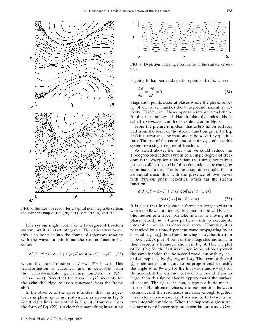
For integrable systems, an orbit either eventually re-turns to itself, in which case we have a periodic orbit, orit maps out a curve, which is an example of an invariantset. The latter case is typical, as illustrated in Fig. 6. Innonintegrable or chaotic systems this is not true, as isillustrated in Figs. 7(a) and 7(b), where it is seen thatorbits make ‘‘erratic’’ patterns.
Now what about the fluid mechanics illustration? Canchaos exist? How can we have a two-degree-of-freedomsystem when we have only the two spatial coordinates,say (u ,J)? The answer is that explicit time dependencein c, the extra half degree of freedom, is enough forchaos. There is, in fact, a trick for puffing up a1 1
2-degree-of-freedom system and making it look like a
6See Wintner (1947), which contains references to severaloriginal papers.
FIG. 5. Depiction of invariant circle streamlines for an azi-muthally symmetric flow.
Rev. Mod. Phys., Vol. 70, No. 2, April 1998
two-degree-of-freedom system, and vice versa.Let s correspond to a fake time variable, set t5f ,
where f is going to be a new canonical coordinate, anddefine a new Hamiltonian by
H~u ,J ,f ,I !52c~u ,J ,f!1I . (19)
The equations of motion for this Hamiltonian are
du
ds5
]H
]J52
]c
]J,
dJ
ds52
]H
]u5
]c
]u, (20)
df
ds5
]H
]I51,
dI
ds52
]H
]f5
]c
]f. (21)
The first of Eqs. (21) tells us that f5s1s05t ; we sets050. Thus we obtain what we already knew, namely,that f5t and that Eqs. (20) give the correct equations ofmotion. What is the role of the second of Eqs. (21)? Thisequation merely tells us that I has to change so as tomake H5const.
The above trick becomes particularly useful when c isa periodic function of time: c(u ,J ,t)5c(u ,J ,t1T). Inthis case it makes sense to identify f1T with f , becausethe velocity field is the same at these points. With thisidentification done, it is clear that a surface of section isobtained by plotting (u ,J) at intervals of T .
One can construct 1 12-degree-of-freedom Hamiltonian
systems from two-degree-of-freedom Hamiltonian sys-tems by using one of the configuration-space coordinatesas a time variable. We leave the details of this calcula-tion as an exercise.
Now suppose the stream function is composed of anazimuthal shear flow plus a propagating wave:
c~J ,u ,t !5c0~J !1c1~J !cos@m1~u2v1t !# , (22)
where m1PN (i.e., m1 is a natural number) and c1 isassumed small in comparison to c0. Here c0(J) repre-sents the azimuthal background shear flow and the sec-ond term represents the wave, with c1, m1, and v1 beingthe radial eigenfunction, mode number, and frequencyof the wave, respectively.
FIG. 6. Surface of section for an integrable system.
473P. J. Morrison: Hamiltonian description of the ideal fluid
This system might look like a 1 12-degree-of-freedom
system, but it is in fact integrable. The easiest way to seethis is to boost it into the frame of reference rotatingwith the wave. In this frame the stream function be-comes
c8~J8,u8,t !5c0~J8!1c1~J8!cos~m1u8!2v1J8, (23)
where the transformation is J85J , u85u2v1t . Thistransformation is canonical and is derivable fromthe mixed-variable generating function F(u ,J8)5J8(u2v1t). Note that the term 2v1J8 accounts forthe azimuthal rigid rotation generated from the frameshift.
In the absence of the wave it is clear that the trajec-tories in phase space are just circles, as shown in Fig. 5(or straight lines, as plotted in Fig. 6). However, fromthe form of Eq. (22) it is clear that something interesting
FIG. 7. Surface of section for a typical nonintegrable system,the standard map of Eq. (26) at (a) k50.80; (b) k'0.97.
Rev. Mod. Phys., Vol. 70, No. 2, April 1998
is going to happen at stagnation points, that is, where
]c
]u85
]c
]J850. (24)
Stagnation points occur at places where the phase veloc-ity of the wave matches the background azimuthal ve-locity. Here a critical layer opens up into an island chain.In the terminology of Hamiltonian dynamics this iscalled a resonance and looks as depicted in Fig. 8.
From the picture it is clear that orbits lie on surfacesand from the form of the stream function given by Eq.(23) it is clear that the motion can be solved by quadra-ture. The use of the coordinate u85u2v1t reduces thissystem to a single degree of freedom.
As noted above, the fact that we could reduce the1 1
2-degree-of-freedom system to a single degree of free-dom is the exception rather than the rule; generically itis not possible to get rid of time dependence by changingcoordinate frames. This is the case, for example, for anazimuthal shear flow with the presence of two waveswith different phase velocities, which has the streamfunction
c~J ,u ,t !5c0~J !1c1~J !cos@m1~u2v1t !#
1c2~J !cos@m2~u2v2t !# . (25)
It is clear that in this case a frame no longer exists inwhich the flow is stationary. In general there will be cha-otic motion of a tracer particle. In a frame moving at aphase velocity v1 a tracer particle wants to execute itsintegrable motion, as described above. However, it isperturbed by a time-dependent wave propagating by ata speed uv12v2u. In a frame moving at v2 the situationis reversed. A plot of both of the integrable motions, intheir respective frames, is shown in Fig. 9. This is a plotof Eq. (23) for the first wave superimposed on a plot ofthe same function for the second wave, but with c1, m1,and v1 replaced by c2, m2, and v2. The form of c1 andc2 is chosen in this figure to be proportional to sech2;the angle u8 is u2v1t for the first wave and u2v2t forthe second. If the distance between the island chains islarge, then this figure closely approximates the surfaceof section. The figure, in fact, suggests a basic mecha-nism of Hamiltonian chaos, the competition betweenresonances. If the resonances are close enough togethera trajectory, in a sense, flips back and forth between thetwo integrable motions. When this happens a given tra-jectory may no longer map out a continuous curve. Gen-
FIG. 8. Depiction of a single resonance in the surface of sec-tion.

474 P. J. Morrison: Hamiltonian description of the ideal fluid
erally separatrices become fuzzy, but some continuouscurves still exist, as shown in Fig. 7.
As stated above, Fig. 9 is not a surface of section,because the resonances were plotted independently, butif they are far apart and the amplitudes of the reso-nances are both small it looks about right. To see thereal surface of section one could integrate the differen-tial equations numerically.7 Instead of doing this you canconsider the following toy, actually a serious toy, calledthe standard map (which is sometimes called theChirikov-Taylor map):
un118 5un81Jn118 ,
Jn118 5Jn82k sin~un8 !, (26)
where Jn8 and un8 are computed modulo 2p . This is anexample of an area-preserving map; it was, in fact, usedto obtain Figs. 6, 7(a), and 7(b). Area-preserving mapsare nice because the surface of section can be obtainedwithout having to iterate differential equations. Impor-tantly, the standard map describes generic behavior ofHamiltonian systems near resonances—it is the proto-type of area-preserving maps.
I recommend that you examine the standard mapstarting from k50, gradually increasing k . The case inwhich k50 was shown in Fig. 6, which clearly indicatesintegrable behavior. For kÞ0 some of the invariant sets(continuous curves) are broken. As k → 0 the measureof invariant sets approaches unity. This is in essence thecelebrated Kolmogorov-Arnold-Moser (KAM) theo-rem. For larger k more and more curves are broken, butsome still exist [see Fig. 7(a) where k50.80 and Figs.7(b) where k51.2]. At a critical value of kc'0.97,curves that span 0,u8<2p no longer exist. The criticalvalue kc was calculated by Greene (1979) [see also Fal-colini and de la Llave (1992)] to many decimal places.
The question of when the last continuous curvebreaks is an important one in Hamiltonian dynamics
7To do this one can use standard Runge-Kutta packages.However, more sophisticated symplectic integration algorithmsexist. See, for example, Sanz-Serna and Calvo (1994), Kueny(1993), and Kueny and Morrison (1995).
FIG. 9. Depiction of two resonances in the surface of section.
Rev. Mod. Phys., Vol. 70, No. 2, April 1998
theory. In particular, it is of importance in the passiveadvection fluid mechanics problem since these curvesare barriers to transport. One is interested in when thesecurves break as the sizes and positions of the resonanceschange. The method developed by Greene gives a pre-cise answer to this question, but requires some effort. Asimple but rough criterion that yields an estimate forwhen the continuous curves between two resonancescease to persist is given by the Chirikov overlap crite-rion. According to this criterion the last curve separatingtwo resonances will be destroyed when the sum of thehalf-widths of the two resonances (calculated indepen-dently) equals the distance between the resonances; thatis,
W1
21
W2
25uJ182J28u, (27)
where W1 and W2 denote the widths of the resonanceswhile J18 and J28 denote their positions. This criterion isstraightforward to apply and usually gives reasonable re-sults. However, it must be borne in mind that it is only arough estimate and as such has limitations. As notedabove, more sophisticated criteria exist.
The study of two-degree-of-freedom Hamiltonian sys-tems is a richly developed yet still open area of research.Unfortunately, in a single lecture it is only possible toscratch the surface and, it is hoped, whet your appetite.Conspicuously absent from this lecture is any discussionof the notions of universality and renormalization (see,for example, MacKay, 1982 or del-Castillo-Negreteet al., 1997). There is much to be learned from the ref-erences we have cited.
E. ‘‘Diffusion’’: Three degrees of freedom
In closing we mention something about three-degree-of-freedom systems. For these systems the invariant setsthat are remnants of the integrable N-tori do not dividethe phase space. For three-degree-of-freedom systemsthe phase space is six dimensional and the correspond-ing three-dimensional invariant tori do not isolate re-gions. Because of this, trajectories are not confined andcan wander around the tori. This phenomenon is gener-ally called Arnold diffusion. A cartoon of this is shownin Fig. 10.
FIG. 10. Cartoon depicting the motion around invariant tori insystems with greater than two degrees of freedom.

475P. J. Morrison: Hamiltonian description of the ideal fluid
There is a great deal of literature dealing with thechaotic advection of a passive tracer in two-dimensionalfluid systems. These studies typically involve modelstream functions that are time periodic and hence arenonintegrable. For these systems the diffusion phenom-enon mentioned above cannot occur. However, it is pos-sible that the solution of Eq. (1) is not periodic, butquasiperiodic, a special case of which is represented bythe following:
c~u ,J ,t !52f~u ,J ,v2t ,v3t !, (28)
where f is a function that satisfies
f~u ,J ,v2t ,v3t !5f~u ,J ,v2t12p ,v3t !
5f~u ,J ,v2t ,v3t12p!. (29)
If v2 /v3 is irrational, then c is not periodic.One can puff up a system with a Hamiltonian of the
form of Eq. (28) into a three-degree-of-freedom systemby a technique similar to that described above. Letu5 :u1 , J5 :J1 , define
H~u1 ,J1 ,u2 ,J2 ,u3 ,J3!5f~u1 ,J1 ,u2 ,u3!1v2J2
1v3J3 , (30)
and introduce the fake time s as before. Note that thelast two terms of Eq. (30) are just the Hamiltonian fortwo linear oscillators in action-angle form, but here theyare coupled to each other and to oscillator ‘‘1’’ throughf . Hamilton’s equations are
du1
ds5
]f
]J1,
du2
ds5v2 ,
du3
ds5v3 , (31)
dJ1
ds52
]f
]u1,
dJ2
ds52
]f
]u2,
dJ3
ds52
]f
]u3. (32)
It is clear how the last two equations of (31) can beintegrated and thus the system can be collapsed backdown. The last two equations of (32) guarantee that J2and J3 will vary so as to make H conserved.
The kind of quasiperiodic system treated in this sub-section is undoubtedly relevant for the study of trans-port in two-dimensional fluids. Solutions of Eq. (1) arelikely to be closer to quasiperiodic than periodic. Astream function that describes an azimuthally symmetricshear flow plus three waves with different speeds is qua-siperiodic. Transport in such systems and their generali-zation to more frequencies is not well understood. (See,for example, Wiggins, 1992.)
III. FUNCTIONAL CALCULUS, TWO ACTION PRINCIPLESOF MECHANICS, AND THE ACTION PRINCIPLEAND CANONICAL HAMILTONIAN DESCRIPTIONOF THE IDEAL FLUID
This lecture is devoted to developing techniques thatare needed to describe infinite-dimensional Hamiltoniansystems, and then to using these techniques to describethe canonical Hamiltonian description of the ideal fluidin terms of so-called Lagrangian or material variables.Specifically, in Sec. III.A techniques of functional calcu-
Rev. Mod. Phys., Vol. 70, No. 2, April 1998
lus are presented, in Sec. III.B two traditional actionprinciples of classical mechanics are reviewed along withtheir connection to Hamilton’s equations, and in Sec.III.C the action principle and Hamiltonian descriptionof the fluid are treated in detail.
A. Functional calculus
A functional is a map that takes functions into realnumbers. Describing them correctly requires defining afunction space, which is the domain of the functional,and the rule that assigns the real number. Like ordinaryfunctions, functionals have notions of continuity, differ-entiability, the chain rule, etc. In this subsection we shallnot be concerned with rigor, but with learning how toperform various formal manipulations.8
As an example of a functional consider the kineticenergy of a constant-density, one-dimensional, boundedfluid:
T@u#5 12 E
x0
x1r0u2dx . (33)
Here T is a functional of u which is indicated by the @ #notation, a notation that we use in general to denotefunctionals. The function u(x) is the fluid velocity,which is defined on xP@x0 ,x1# , and r0 is a constant fluiddensity. Given a function u(x) we could put it into Eq.(33), do the integral, and get a number.
We would like to know in general how the value of afunctional K@u# changes as u(x) changes a little, sayu(x)→u(x)1e du(x), where u1e du must still be inour domain. The first-order change in K induced by duis called the first variation, dK , and is given by
dK@u ;du# :5 lime→0
K@u1edu#2K@u#
e
5d
deK@u1edu#U
e50
5 :Ex0
x1du
dK
du~x !dx5 : K dK
du,du L . (34)
We shall assume that the limit exists and that there areno problems with the equalities above; later, however,we shall give an exercise in which something ‘‘interest-ing’’ happens.
The notation dK@u ;du# is used because there is a dif-ference in the behavior of the two arguments: generallydK is a linear functional in du , but not so in u . Thequantity dK/du(x) of Eq. (34) is the functional deriva-tive of the functional K . This notation for the functionalderivative is chosen since it emphasizes the fact that
8For further details, on a level roughly consistent with thatgiven here, see Courant and Hilbert (1953), Chapter IV, andGelfand and Fomin (1963).

476 P. J. Morrison: Hamiltonian description of the ideal fluid
dK/du is a gradient in function space. The reason whythe arguments of u are sometimes displayed will becomeclear below.
For the example of Eq. (33) the first variation is givenby
dT@u ;du#5Ex0
x1r0u dudx , (35)
and hence the functional derivative is given by
dT
du5r0u . (36)
To see that the functional derivative is a gradient, letus take a sidetrack and consider the first variation of afunction of n variables, f(x1 ,x2 , . . . ,xn)5f(x):
df~x ;dx !5(i51
n]f~x !
]xidxi5 :¹f•dx . (37)
It is interesting to compare the definition of Eq. (37)with the last definition of Eq. (34). The • in Eq. (37) isanalogous to the pairing ^ , &, while dx is analogous todu . In fact, the index i is analogous to x , the argumentof u . Finally, the gradient ¹f is analogous to dK/du .
Consider now a more general functional, one of theform
F@u#5Ex0
x1F~x ,u ,ux ,uxx , . . . !dx , (38)
where F is an ordinary, sufficiently differentiable, func-tion of its arguments. Note ux :5du/dx , etc. The firstvariation of Eq. (38) yields
dF@u ;du#5Ex0
x1S ]F]u
du1]F]ux
dux
1]F
]uxxduxx1••• Ddx , (39)
which upon integration by parts becomes
dF@u ;du#5Ex0
x1duS ]F
]u2
d
dx
]F]ux
1d2
dx2
]F]uxx
2••• Ddx
1S ]F]ux
du1••• D Ux0
x1
. (40)
Usually the variations du are chosen so that the lastterm, the boundary term, vanishes; e.g., du(x0)5du(x1)50, dux(x0)5dux(x1)50, etc. Sometimes theboundary term vanishes without a condition on du be-cause of the form of F. When this happens the boundaryconditions are called natural. Assuming, for one reasonor the other, that the boundary term vanishes, Eq. (40)becomes
dF@u ;du#5 K dF
du,du L , (41)
Rev. Mod. Phys., Vol. 70, No. 2, April 1998
where
dF
du5
]F]u
2d
dx
]F]ux
1d2
dx2
]F]uxx
2••• . (42)
The main objective of the calculus of variations is theextremization of functionals. A common terminology isto call a function u , which is a point in the domain, anextremal point if dF@u#/duuu5u50. It could be a maxi-mum, a minimum, or an inflection point. If the extremalpoint u is a minimum or maximum, then such a point iscalled an extremum.
The standard example of a functional that depends onthe derivative of a function is the arc-length functional,
L@u#5Ex0
x1A11ux2 dx . (43)
We leave it to you to show that the shortest distancebetween two points is a straight line.
Another example is the functional defined by evaluat-ing the function u at the point x8. This can be written as
u~x8!5Ex0
x1d~x2x8!u~x !dx , (44)
where d(x2x8) is the Dirac delta function and wherewe have departed from the @ # notation. Applying thedefinition of Eq. (34) yields
du~x8!
du~x !5d~x2x8!. (45)
This is the infinite-dimensional or continuum analog of]xi /]xj5d ij , where d ij is the Kronecker delta function.Equation (45) shows why it is sometimes useful to dis-play the argument of the function in the functional de-rivative.
The generalizations of the above ideas to functionalsof more than one function and to more than a singlespatial variable are straightforward. An example is givenby the kinetic energy of a three-dimensional compress-ible fluid,
T@r ,v#5 12 E
Drv2 d3x , (46)
where the velocity has three rectangular componentsv5(v1 ,v2 ,v3) that depend upon x5(x1 ,x2 ,x3)PD andv25v•v5v1
21v221v3
2. The functional derivatives are
dT
dv i5rv i ,
dT
dr5
v2
2. (47)
We shall use these later.For a more general functional F@c# , where
c(x)5(c1,c2, . . . ,cn) and x5(x1 ,x2 , . . . ,xn), the ana-log of Eq. (34) is
dF@c ;dc#5ED
dc i
dF
dc i~x !dnx5 : K dF
dc,dc L . (48)
As an exercise consider the pathological functional
P@c#5E21
1P~c1 ,c2! dx , (49)

477P. J. Morrison: Hamiltonian description of the ideal fluid
where
P5H c1c22
c121c2
2 if c1,2Þ0,
0 if c1,250.
(50)
Calculate dP@0,0;dc1 ,dc2# . Part of this problem is tofigure out what the problem is.
Next, we consider the important functional chain rule,which is a simple idea that underlies a great deal of lit-erature relating to the Hamiltonian structure of fluidsand plasmas.
Suppose we have a functional F@u# and we know u isrelated to another function w by means of a linear op-erator
u5Ow . (51)
As an example, u and w could be real-valued functionsof a single variable x , and
O:5 (k50
n
ak~x !dk
dxk , (52)
where, as usual, u , w , and ak have as many derivatives asneeded. We can define a functional of w by inserting Eq.(51) into F@u# :
F@w# :5F@u#5F@Ow# . (53)
Equating variations yields
K dF
dw,dwL 5 K dF
du,du L , (54)
where the equality makes sense if du and dw are con-nected by Eq. (51), i.e.,
du5Odw , (55)
where we assume an arbitrary dw induces a du .Inserting Eq. (55) into Eq. (54) yields
K dF
dw,dwL 5 K dF
du,Odw L 5 : KO†
dF
du,dw L , (56)
where O† is the formal adjoint of O. The DuBois-Reymond lemma of the calculus of variations states thatif dw is arbitrary, then Eq. (56) implies
dF
dw5O†
dF
du. (57)
This lemma is proven by assuming that Eq. (57) does nothold at some point x , selecting dw to be localized aboutthe point x , and establishing a contradiction. A physicistwould just set dw equal to the Dirac delta function toobtain the result.
Notice that nowhere did we assume that O wasinvertible—it need not be for the chain rule to work inone direction. This is because, in the sense displayed
Rev. Mod. Phys., Vol. 70, No. 2, April 1998
above, functionals transform in the other direction.Clearly the transformation of Eq. (51) is a special case,in that the two functions u and w are linearly related.However, if u depends nonlinearly upon w we can stillobtain a relation of the form of Eq. (57). We shall dem-onstrate this in the more general case for a functionalF@c# , where c is related to x5(x1,x2, . . . ,xm) in anarbitrary, possibly nonlinear and noninvertible, way:
c i5c i@x# , i51,2, . . . ,n . (58)
This @ # notation could be confusing, since we have usedit to denote functionals, but since we have already statedthat c and x are functions there should be no confusion.A variation of c induced by x requires linearization ofEq. (58), which we write as
dc i5dc i
dx@x ;dx# , (59)
or simply, since dc/dx is a linear operator on dx , as
dc i5dc i
dx j dx j, (60)
where j51,2, . . . ,m . Inserting Eq. (60) into Eq. (54) im-plies
K dF
dx,dx L 5 K S dc
dx D † dF
dc,dx L , (61)
whence it is seen that
dF
dx j 5S dc i
dx j D † dF
dc i . (62)
Here we have dropped the overbar on F , as is com-monly done. In Eq. (62) it is important to rememberthat d(function)/d(function) is a linear operator actingto its right, as opposed to d(functional)/d(function),which is a gradient.
As an example consider functionals that depend uponthe two components of the velocity field for an incom-pressible fluid in two dimensions, u(x ,y) and v(x ,y).These are linearly related to the stream function c byu52]c/]y and v5]c/]x . For this case Eq. (59) be-comes
du5du
dcdc52
]
]ydc ,
dv5dvdc
dc5]
]xdc , (63)
and
dF
dc5
]
]y
dF
du2
]
]x
dF
dv. (64)
Now consider the second variation, d2F , and secondfunctional derivative, d2F/dcdc . Since the first varia-

478 P. J. Morrison: Hamiltonian description of the ideal fluid
tion, dF@c ;dc# , is a functional of c , a second variationcan be made in this argument:
d2F@c ;dc ,dc#5d
dhdF@c1hdc ;dc#U
h50
5 :ED
dc id2F
dc idc jdc j dnx
5 : K dc ,d2F
dcdcdc L . (65)
Observe that d2F is a bilinear functional in dc and dc .If we set dc5dc we obtain a quadratic functional.Equation (65) defines d2F/dcdc , which is an operatorthat acts linearly on dc but depends nonlinearly on c .This operator possesses a symmetry analogous to theinterchange of the order of second partial differentia-tion. To see this observe
d2F@c ;dc ,dc#5]2
]h]eF@c1hdc1edc#U
e50,h50
.
(66)
Since the order of differentiation in Eq. (66) is immate-rial it follows that
S d2F
dc idc jD †
5d2F
dc jdc i. (67)
This relation is necessary for establishing the Jacobiidentity of noncanonical Poisson brackets.
As an example consider the second variation of thearc-length functional of Eq. (43). Performing the opera-tions of Eq. (66) yields
d2L@u ;du ,du#5Ex0
x1dux
1
~11ux2!3/2
duxdx . (68)
Thus
d2L
du25
d
dx
21
~11ux2!3/2
d
dx. (69)
For an important class of function spaces, one canconvert functionals into functions of a countably infinitenumber of arguments. This is a method for provingtheorems concerning functionals and can also be usefulfor establishing formal identities. One way to do thiswould be to convert the integration of a functional into asum by finite differencing. Another way to do this, forexample for functionals of the form of Eq. (38), is tosuppose @x0 ,x1#5@2p ,p# and expand in a Fourier se-ries,
u~x !5 (k52`
`
uk eikx. (70)
Upon inserting Eq. (70) into Eq. (38) one obtains anexpression for the integrand, which is, in principle, aknown function of x . Integration then yields a functionof the Fourier amplitudes, uk . Thus we obtain
Rev. Mod. Phys., Vol. 70, No. 2, April 1998
F@u#5F~u0 ,u1 ,u21 , . . . !. (71)
In closing this discussion of functional calculus weconsider a functional, one expressed as a function of aninfinite number of arguments, that demonstrates an ‘‘in-teresting’’ property. The functional is given by
F~x1 ,x2 , . . . !5 (k51
`
~ 12 akxk
22 14 bkxk
4 !, (72)
where the domain of F is composed of sequences $xk%,and the coefficients are given by
ak51
k6, bk5
1
k2. (73)
Assuming that Eq. (72) converges uniformly, the firstvariation yields
dF5 (k51
`
~akxk2bkxk3 !dxk , (74)
which has three extremal points,
xk~0 !50, xk
~6 !56~ak /bk!1/2, (75)
for all k . It is the first of these that will concern us. Thesecond variation evaluated at xk
(0) is
d2F5 (k51
`
ak~dxk!2, (76)
where we assume Eq. (74) converges uniformly for xkand dxk . Since ak.0 for all k , Eq. (76) is positive defi-nite; i.e.,
d2F.0 for dxkÞ0, for all k . (77)
However, consider DF defined by
DF5F~x ~0 !1Dx !2F~x ~0 !!
5 (k51
`
@ 12 ak~Dxk!22 1
4 bk~Dxk!4# , (78)
which we evaluate at
Dxk5H 1m
, k5m ,
0, kÞm ,(79)
and obtain
DF,0, (80)
provided m.1. Since m can be made as large as desired,we have shown that inside any neighborhood of x (0), nomatter how small, DF,0. Therefore this extremal pointis not a minimum — even though d2F is positive defi-nite.
A sufficient condition for proving that an extremalpoint is an extremum is afforded by a property known asstrong positivity. If c is an extremal point and the qua-dratic functional d2F@c ;dc# satisfies
d2F@c ;dc#>cidci2,

479P. J. Morrison: Hamiltonian description of the ideal fluid
where c5const.0 and i i is a norm defined on thedomain of F , then d2F@c ;dc# is strongly positive. This issufficient for c to be a minimum. We leave it to you toexplain why the functional F(x1 ,x2 , . . . ) is not stronglypositive. This example points to a mathematical techni-cality that is encountered when proving stability by Li-apunov’s method (see Sec. VI).
B. Two action principles of mechanics
Physicists have had a long-lasting love affair with theidea of generating physical laws by setting the derivativeof some functional to zero. This is called an action prin-ciple. The most famous action principle is Hamilton’sprinciple, which produces Lagrange’s equations of me-chanics upon variation. One reason action principles areappreciated is that they give a readily covariant theory,and means have been developed for building in symme-tries. However, it should be pointed out that the use ofcontinuous symmetry groups in this context is only alimited part of a deep and beautiful theory that was ini-tiated by Sophus Lie and others. Perhaps the most con-vincing deep reason for the use of action principles is thecleanliness and utility of Feynman’s path-integral formu-lation. The utility of action principles should not be un-derstated. Indeed, they provide a good starting place formaking approximations. However, a quote from Trues-dell (1966) cannot be resisted:
‘‘A fully conservative situation can be described by anaction principle, which has the advantage of making thetheory accessible also to physicists.’’
In any event, Hamilton’s principle is an importantprototype upon which modern theories are in part built.Shortly, we shall show how this story goes for the idealfluid, but first we review some mechanics. [See Saletanand Cromer (1971) or Sudarshan and Mukunda (1974)for standard presentations.]
One approach to producing the equations of motionfor a mechanics problem is first to identify the configu-ration space Q with coordinates q5(q1 ,q2 , . . . ,qN).Then, based on physical intuition, write down the kineticand potential energies, T and V , respectively. The equa-tions of motion then follow upon setting the functionalderivative of the following action functional to zero:
S@q#5Et0
t1L~q ,q ,t ! dt , (81)
where L :5T2V is the Lagrangian function. The func-tions q(t) over which we are extremizing must satisfythe fixed end conditions q(t0)5q0 and q(t1)5q1. Thusdq(t0)5dq(t1)50. The functional derivative relations
dS@q#
dqi50 (82)
imply Lagrange’s equations,
]L
]qi5
d
dt
]L
]q i. (83)
Rev. Mod. Phys., Vol. 70, No. 2, April 1998
This is Hamilton’s principle.Since for particles in rectangular coordinates9 usually
T5 12 (
i51
N
mi~ q i!2, V5V~q !, (84)
Eqs. (83) yield
miqi52]V
]qi. (85)
This is just Newton’s second law with a conservativeforce. You will notice that Hamilton’s principle does notyield Hamilton’s equations—one way to get them is viathe Legendre transformation.
The Legendre transformation is a trick for transferringfunctional dependence. Generally it is used in physicswhen one has a sort of ‘‘fundamental’’ function that de-scribes a theory, whether it be a thermodynamic poten-tial or, as is the case here, a Lagrangian. The Legendretransformation has a nice geometric interpretation, butwe shall skip this. Here we shall use it to transform theN second-order differential equations of (85) into the2N first-order equations of Hamilton.
Define a quantity pi :5]L/]q i, which is the canonicalmomentum, and consider
H~q ,p ,q ,t !:5piqi2L~q ,q ,t !. (86)
Now we ask the question: How does H change if weindependently change q , q , p , and t a little? Evidently
dH5]H
]qidqi1
]H
]q idq i1
]H
]pidpi1
]H
]tdt
52]L
]qidqi1S pi2
]L
]q iD dq i1q idpi
2]L
]tdt . (87)
The first thing to notice is that if dq5dp5dt50, i.e., weonly vary dq , then dH50, since pi5]L/]q i. This meansH is independent of q , so we drop the overbar and writeH(q ,p ,t). Equating the remaining coefficients of thevariations yields
]H
]qi52
]L
]qi,
]H
]pi5q i,
]H
]t52
]L
]t. (88)
Lagrange’s equations, (83), together with the defini-tion of pi and the middle equation of (88), give Hamil-ton’s equations:
p i52]H
]qi, q i5
]H
]pi. (89)
9More precisely the kinetic energy contains h ijqiq j, where the
metric h ij :5d ij and its inverse can be used to raise and lowerindices.

480 P. J. Morrison: Hamiltonian description of the ideal fluid
In order to calculate H(p ,q ,t) explicitly one usespi5]L/]q i to solve for q5q(p) and then inserts thisinto Eq. (86). This requires L to be convex in q . Sincethere exist important physical cases in which L is notconvex, Dirac and others developed a theory to handlethis. An interesting application of Dirac’s constrainttheory for filtering out fast motion in geophysical fluiddynamical models has been developed by Salmon(1988a).
Now consider another action principle, which is some-times called the phase-space action. This one, which di-rectly yields Hamilton’s equations, is given by
S@q ,p#5Et0
t1@piq
i2H~q ,p ,t !# dt , (90)
where S is a functional of q and p , independently. Theend conditions are q(t0)5q0 and q(t1)5q1, i.e., q isfixed as before. However, the boundary condition on pis natural in that nothing is required of it at the ends.One has a sort of ‘‘clothesline’’ boundary condition asdepicted in Fig. 11, where the curve is free to slide alongthe lines of constant q in the p direction.
Variation of S with respect to q and p yields, respec-tively,
p i52]H
]qi, q i5
]H
]pi. (91)
Thus the phase-space action directly yields Hamilton’sequations as the extremal condition.
C. Action principle and canonical Hamiltonian descriptionof the ideal fluid in Lagrangian or material variables
Now we are in a position to talk about the action forfluid mechanics,10 but we are going to do so in terms of
10An action principle for the ideal fluid dates back toLagrange (1788), although of course he was unaware of thethermodynamics that we shall include. More modern refer-ences with generalizations include Serrin (1959), Eckart(1960), Newcomb (1962), and Salmon (1982, 1988b).
FIG. 11. Clothesline boundary conditions for the phase-spaceaction principle.
Rev. Mod. Phys., Vol. 70, No. 2, April 1998
variables that might be new to you. Often, fluid mechan-ics is taught entirely in terms of Eulerian variables. Inwhat follows, Lagrangian variables, or as they are some-times called, material variables, will be central.
The idea we are going to pursue is a simple one. If afluid is described as a collection of fluid particles or ele-ments, then both the Hamiltonian and the Lagrangianformalism that we have described above can be adaptedto describe the ideal fluid. The adaptation requires anextension to an infinite number of degrees of freedom inorder to describe a continuum of fluid elements. Thismeans that a fluid element is shrunk to zero size and thatthere is one for each point of the fluid. This is an ideali-zation, since in reality fluid elements do not exist: if theywere of macroscopic size, they would not maintain theirintegrity forever, and if they were of microscopic size,we would be outside the realm of fluid mechanics. How-ever, there exists a precise Eulerian state correspondingto a Lagrangian state. It should be kept in mind that theabove limitations apply to the fluid description in gen-eral, whether it be in Lagrangian or Eulerian variables.
Suppose the position of a fluid element, referred to afixed rectangular coordinate system, is given by
q5q~a ,t !, (92)
where q5(q1 ,q2 ,q3). This is the material or Lagrangianvariable. Here a5(a1 ,a2 ,a3) could be any label11 thatidentifies a fluid particle, but below it will be taken to bethe position of the fluid particle at time t50 in rectan-gular coordinates. The quantities qi(a ,t) are coordinatesfor the configuration space Q, which is in fact a functionspace because in addition to the three indices i there isthe continuum label a . We assume that a varies over afixed domain D , which is completely filled with fluid,and that the functions q map D onto itself. We shallassume that as many derivatives of q with respect to a asneeded exist, but we shall not say more about Q; in fact,not that much is known about the solution space for the3D fluid equations in Lagrangian variables. At this stagewe shall assume that the configuration space has beenspecified and proceed to discuss the potential energy ofthe fluid.
The fluid approximation assumes local thermody-namic equilibrium in spite of the fact that fluid motion isin general not quasistatic. Potential energy is stored interms of pressure and temperature. More precisely, weadapt the energy representation of thermodynamics inwhich the extensive energy is treated as a function of theextensive variables, viz., the entropy and the volume.For a fluid it is convenient to consider the energy perunit mass, which we denote by U to be a function of theentropy per unit mass, s , and the mass density, r . Theinverse of the latter quantity is a measure of the volume.The intensive quantities, pressure and temperature, areobtained as follows:
11Note that the freedom to relabel particles is associated withthe Casimir invariants, which are discussed below. See Calkin(1963), Newcomb (1967), Bretherton (1970), Ripa (1981),Salmon (1982), and Padhye and Morrison (1996a, 1996b).

481P. J. Morrison: Hamiltonian description of the ideal fluid
T5]U
]s~s ,r!, p5r2
]U
]r~s ,r!. (93)
The second of equation (93) is a bit peculiar—it arisesbecause the volume, the usual thermodynamic variable,is proportional to r21. Special choices for U producespecific thermodynamics for fluid flow.12
The quantities r and s are in fact Eulerian variables,which we must, in order to move ahead, describe interms of Lagrangian variables. With this goal in mind,let us diverge for a moment and discuss the Lagrangian-Eulerian map. The difference between the two types ofvariables can be elucidated by describing two ways ofwatching fish. In the Eulerian picture one stays at apoint and watches whatever fish happen by; in the La-grangian picture one picks out a particular fish andkeeps track of where it goes. Note that this analogy getsbetter if the fish are very small, neutrally buoyant, anddead.
Call r the spatial variable, i.e., the Eulerian point ofobservation. The Eulerian density is then related to theLagrangian variable q as
r~r ,t !5ED
d„r2q~a ,t !…r0~a ! d3a . (94)
Here d(r2q) is a three-dimensional Dirac delta func-tion and r0(a) is an initial configuration of mass densityascribed to the particle labeled by a . It is akin to know-ing the mass of the particle labeled by i in conventionalparticle mechanics.
Equation (94) embodies mass conservation. This canbe seen by using a property of the d function,d„f(x)…5d(x2x0)/uf8(x0)u, where x0 is the only placewhere f(x0)50. In three dimensions this yields
r~r ,t !5r0~a !
J~a ,t !Ua5q21~r ,t !
, (95)
where the Jacobian J5det(]qi/]aj). That this is localmass conservation follows from
r d3q5r0 d3a , (96)
where d3a is an initial volume element that maps intod3q at time t , and d3q5J d3a . (When integrating overD we shall replace d3q by d3r .)
In addition to the mass ascribed to a fluid particle, onecould ascribe other quantities, e.g., color, smell, or whathave you. In the ideal fluid, the entropy per unit mass sis such a quantity. We suppose that initially s5s0(a)and that it remains so. A form similar to Eq. (94) corre-sponding to this statement is
s~r ,t !5ED
s0~a !d„r2q~a ,t !…d3a , (97)
12For barotropic or isentropic flow, U depends only on r . Foran ideal monoatomic gas U(r ,s)5crg21exp(as), where c , g ,and a are constants. See, for example, Serrin (1959) for a dis-cussion of equations of state.
Rev. Mod. Phys., Vol. 70, No. 2, April 1998
where s(r ,t)5r(r ,t)s(r ,t) is the entropy per unit vol-ume and s05r0(a)s0(a). Thus the counterpart of Eq.(95) is
s~r ,t !5s0~a !ua5q21~r ,t ! . (98)
This is merely the statement that the quantity s stays puton a fluid particle.
Completing the Lagrange-Euler map requires thespecification of the Eulerian velocity field, somethingthat is not needed now, but that we record here for laterreference. By now you will have noticed that the Euler-Lagrange map naturally takes the Lagrangian variablesinto Eulerian densities. Thus we consider the momen-tum density M :5rv . A form for M similar to Eqs. (94)and (97) is
M~r ,t !5ED
q~a ,t !d„r2q~a ,t !…r0~a !d3a , (99)
where the • notation now means differentiation with re-spect to time at fixed label a . Performing the integrationproduces the counterpart of Eqs. (95) and (96), viz.,
v~r ,t !5q~a ,t !ua5q21~r ,t ! , (100)
which is the usual relation between the Lagrangian vari-able and the Eulerian velocity field.
Now we can return to our quest for the potential en-ergy. Since the energy per unit volume is given by rU ,the total potential-energy function is evidently
V@q#5ED
r0U~s0 ,r0 /J!d3a . (101)
Observe that Eq. (101) is a functional of q that dependsonly upon J and hence only upon ]q/]a .
The next step required for constructing Hamilton’sprinciple is to obtain an expression for the kinetic-energy functional. This is clearly given by
T@q#5 12 E
Dr0q2d3a , (102)
where we use the shorthand q2:5h ijqiq j. Observe that
Eq. (102) is a functional of q that depends only upon q .From Eqs. (101) and (102) the Lagrangian functional
is obtained,
L@q ,q#5ED
@ 12 r0q22r0U~s0 ,r0 /J!#d3a
5 :EDL~q ,q ,]q/]a ,t !d3a , (103)
where L(q ,q ,]q/]a ,t) is the Lagrangian density. Thusthe action functional is given by
S@q#5Et0
t1L@q ,q#dt5E
t0
t1dtE
D@ 1
2 r0q22r0U#d3a .
(104)
Observe that this action functional is like that forfinite-degree-of-freedom systems, as treated above, ex-cept that the sum over particles is replaced by integra-tion over D , i.e.,

482 P. J. Morrison: Hamiltonian description of the ideal fluid
ED
d3a↔(i
. (105)
The mass of each ‘‘particle’’ of the continuum corre-sponds to r0d3a .
The end conditions for Hamilton’s principle for thefluid are the same as before,
dq~a ,t0!5dq~a ,t1!50. (106)
However, in addition, boundary conditions are neededbecause there is now going to be integration by partswith respect to a . It is assumed that these are such thatall surface terms vanish. Shortly we shall see what thisimplies.
In order to apply Hamilton’s principle, we must func-tionally differentiate Eq. (104); thus it is necessary toknow something about differentiating determinants. Re-call
]qk
]aj
Aki
J 5d ji (107)
where Aki is the cofactor of ]qk/]ai5 :q ,i
k . (Rememberrepeated indices are to be summed.) A convenient ex-pression for Ak
i is given by
Aki 5 1
2 ekjleimn
]qj
]am
]ql
]an, (108)
where e ijk(5e ijk) is the skew-symmetric tensor (den-sity), which vanishes if any two of i ,j ,k are equal; it isequal to 1 if i ,j ,k are unequal and a cyclic permutationof 1,2,3, and is otherwise equal to 21. In functionallydifferentiating Eq. (104) we shall require the followingrelation:
]J]q ,j
i5Ai
j , (109)
which follows from Eq. (107).For Lagrangian density functionals of the form
L(q ,q ,]q/]a ,t), the functional derivative dS/dq(a ,t)50 implies
d
dtS ]L]q iD 1
]
]ajS ]L]q ,j
i D 2]L]qi
50, (110)
provided the surface integral vanishes:
Et0
t1E]D
pdqiAijnjd
2a5Et0
t1E]D
pdq•nd2q . (111)
The equality above follows upon changing from integra-tion over a to integration over q . Clearly the surfaceterm vanishes if any of the following are true on ]D :
~ i! dqi50,
~ ii! p5~r02/J 2!~]U/]r!50,
~ iii! dq•n50,
where p is the pressure and n is a unit normal vector to]D . While all of these possibilities result in the vanishing
Rev. Mod. Phys., Vol. 70, No. 2, April 1998
of the surface term, (i) is clearly more than is necessary,in light of (iii), which merely states that fluid particlesare not forced through the boundary. When D is a boxand periodic boundary conditions are imposed, the van-ishing of the surface term is automatic. When D is ‘‘allspace’’ one has the option (ii), which asserts that thepressure vanishes at infinity. Condition (iii) is the com-mon physical condition.
From Eq. (110) the equation of motion is obtained,
r0q i1Aij ]
]ajS r02
J 2
]U
]r D 50. (112)
Here we have used ]Aij/]aj50, which you can work out
using Eq. (108). Alternatively, upon using Eq. (107), wefind that the equation of motion can be written in theform
r0q j
]qj
]ai1J
]
]aiS r02
J 2
]U
]r D 50. (113)
We leave it to you to show that Eq. (112) can be trans-formed into Eulerian form:
rS ]v]t
1v•¹v D52¹p , (114)
where v5v(r ,t). A useful identity in this regard is
]
]qk5
1J Ak
i ]
]ai. (115)
With Eq. (115) it is clear that Eq. (112) is of the formof Newton’s second law. The Legendre transform fol-lows easily: the canonical momentum density is
p i~a ,t !:5dL
dq i~a !5r0q i, (116)
and
H@p ,q#5E d3a@p•q2L#5E d3aF p2
2r01r0UG .
(117)
Hamilton’s equations are then
p i52dH
dqi, q i5
dH
dp i. (118)
These equations can also be written in terms of the Pois-son bracket,
$F ,G%5E FdF
dq•
dG
dp2
dG
dq•
dF
dp Gd3a , (119)
viz.,
p i5$p i ,H%, q i5$qi,H%. (120)
Here dqi(a)/dqj(a8)5d jid(a2a8) has been used, a re-
lation analogous to ]qj/]qi5d ij for finite systems [recall
Eq. (45)].In conclusion we point out that variational principles
similar to that given above exist for essentially all ideal-

483P. J. Morrison: Hamiltonian description of the ideal fluid
fluid models, including incompressible flow, magnetohy-drodynamics, etc. One can even obtain directly two-dimensional scalar vortex dynamics by consideringconstrained variations, but we shall not pursue this here.
IV. NONCANONICAL HAMILTONIAN DYNAMICSAND EXAMPLES
Preparatory to discussing the Hamiltonian structureof the ideal fluid in terms of Eulerian variables, we nowconsider systems that are Hamiltonian, but written interms of variables (or coordinates) that are not canoni-cal. In Sec. IV.A we describe noncanonical Hamiltoniandynamics for systems with both finite and infinite de-grees of freedom, and in Sec. IV.B we give many ex-amples, which have been culled from the literature. InSec. V we shall show how to derive the noncanonicalHamiltonian description for the ideal fluid from the ca-nonical Lagrangian variable Hamiltonian description ofSec. III.C.
A. Noncanonical Hamiltonian dynamics
Let us start out by playing a sort of game. Suppose wehave a system of ordinary differential equations:
z i5Vi~z !, i51, 2, . . . ,M . (121)
How would you know if this system is a Hamiltoniansystem? If you came upon the equations during researchyou might have some idea based upon the physics, butassume that this is not the case here. What would youdo?
One thing you might try is to check Liouville’s theo-rem. Hamilton’s equations have the property
]q i
]qi1
]p i
]pi5
]2H
]qi]pi
2]2H
]pi]qi50, (122)
from which one can show that phase-space volume isconserved; i.e., if
V~ t !5E )i51
N
dpi dqi, (123)
where the integration is over a volume interior to anarbitrary comoving surface, then
dVdt
50. (124)
The surface may distort, and in general it will do so in amajor way, but the volume inside remains constant. Theanalogous statement for the system of Eq. (121) is in-compressibility of the vector field; i.e.,
]Vi
]zi 50, (125)
whence it follows that
V~ t !5E )i51
N
dzi (126)
Rev. Mod. Phys., Vol. 70, No. 2, April 1998
is constant in time.Suppose Eq. (125) is not true, as is the case for the
following example:
z152z2
3
32z2 ,
z25z1
z2211
. (127)
For this system
] z1
]z11
] z2
]z252
2z1z2
~z2211 !2Þ0. (128)
You would be mistaken if, based on Eq. (128), you con-cluded that Eq. (127) was not Hamiltonian. In fact thissystem is a disguised simple harmonic oscillator. It hasbeen disguised by making a noncanonical coordinatechange, something that we shall discuss below.
So, is there a general method for determining whetheror not a system is Hamiltonian? Probably the answer isno, since one must first find a Hamiltonian, and this re-quires a technique for finding constants of motion.There is no completely general way of doing this.13 Nev-ertheless we can say some things, but to do so we mustinvestigate Hamiltonian systems in arbitrary coordi-nates.
You might wonder, why would equations ever arise innoncanonical variables? Surely the physics would makethings come out right. To the contrary, variables that arethe most physically compelling need not be canonicalvariables. The Eulerian variables that describe ideal con-tinuous media are in general noncanonical. Examples ofsystems that are typically written in terms of noncanoni-cal variables are Liouville’s equation for the dynamics ofthe phase-space density of a collection of particles, theBBGKY hierarchy of kinetic theory, the Vlasov equa-tion of plasma physics, ideal fluid dynamics and variousapproximations thereof, magnetized fluids, . . . : essen-tially every fundamental equation that describes classi-cal media is of this type.
So with the above motivation, let us turn to discussingnoncanonical Hamiltonian dynamics for systems with afinite number of degrees of freedom, using ideas thatextend back (at least) to Sophus Lie. The first step is towrite Hamilton’s equations in covariant form. Thus wedefine
zi5H qi for i51,2, . . . ,N ,
pi2N for i5N11, . . . ,2N . (129)
The zi are coordinates on phase space which we denoteby Z. In terms of the z’s Hamilton’s equations take thecompact form
13Techniques for finding constants of motion do exist, butnecessarily possess limitations. See, for example, Ramani et al.(1989) and references therein.

484 P. J. Morrison: Hamiltonian description of the ideal fluid
z i5Jcij ]H
]zj 5@zi,H# , (130)
where the Poisson bracket is given by
@f ,g#5]f
]zi Jcij ]g
]zj , (131)
with
~Jcij!5S 0N IN
2IN 0ND . (132)
Above, the repeated indices are to be summed over1,2, . . . ,2N . In Eq. (132), 0N is an N3N matrix of zerosand IN is the N3N unit matrix. The subscript c of Jcindicates that the system is written in terms of canonicalcoordinates. It is important to realize that we have onlyrewritten Hamilton’s equations in new notation, albeitin a form that is suggestive.
Now consider a general, time-independent change ofcoordinates
z i5 z i~z !. (133)
The Hamiltonian H transforms as a scalar:
H~z !5H~ z !. (134)
Taking time derivatives of Eq. (133) yields
z l5] z l
]ziz i5
] z l
]ziJc
ij ]H
]zj 5F ] z l
]ziJc
ij ] zm
]zj G ]H
] zm. (135)
Upon defining
Jlm:5] z l
]ziJc
ij ] zm
]zj, (136)
we see that Hamilton’s equations are covariant and thatJlm, which is called the cosymplectic form, transforms asa contravariant tensor of second rank. In the new vari-ables, Hamilton’s equations become
z l5Jlm~ z !]H
] zm5@ z l,H# , (137)
where the Poisson bracket is now given by
@f ,g#5]f
] z lJ lm
]g
] zm. (138)
Notice that in Eq. (137) we have displayed the explicit zdependence in Jlm. This was done to emphasize an im-portant distinction—that between covariance and forminvariance. Equation (136) is a statement of covariance,while a statement of form invariance is given by
Jclm5
] z l
]ziJc
ij ] zm
]zj. (139)
This is, in fact, the (most important) definition of a ca-nonical transformation. Form invariance here meansthat the form of the Jij and hence Hamilton’s equations
Rev. Mod. Phys., Vol. 70, No. 2, April 1998
remains the same. Evidently, the first N of z l are coor-dinates, while the second N are momenta, so it is asimple matter to revert to the usual form of Hamilton’sequations in the new canonical variables z l.
Let us now return to Liouville’s theorem. Taking thedivergence of Eq. (137) yields
] z l
] z l5
]Jlm
] z l
]H
] zm1Jlm
]2H
] z l] zm. (140)
The second term vanishes because Jlm is antisymmetricand ]2H/] z l] zm is symmetric. This is all there is for theusual Liouville’s theorem, since in the canonical case Jlm
is constant, so the first term vanishes. However, forHamilton’s equations written in noncanonical coordi-nates the following is typically (but not necessarily) true:
] z l
] z l5
]Jlm
] z l
]H
] zmÞ0. (141)
This was the situation for our little example of Eq. (127).It might have occurred to you that changing the coor-
dinates may hide but cannot destroy volume preserva-tion. This is clear if we simply change coordinates in Eq.(123):
V~ t !5E J )l51
2N
dzl. (142)
If we include the Jacobian J:5det(]zi/] z j) in the inte-grand, then Liouville’s theorem is still satisfied. There isa nice formula relating J and J , which is obtained bytaking the determinant of Eq. (136) and using the deter-minant product rule:
J51
AdetJ. (143)
Observe that there are many J’s with the same J.Before leaving this discussion of Liouville’s theorem
we mention that even though J is a function of z , it is
still possible for ] z l/] z l50. This can happen because His such that the two vectors of Eq. (141) are perpendicu-lar or it may happen that ]Jlm/] z l50, even though J is afunction of z . The latter case occurs for fluid models andunderlies attempts to describe turbulence by using sta-tistical mechanics concepts (see, for example, Montgom-ery and Kraichnan, 1979).
Now it is clear that the essence of what it means to beHamiltonian does not lie in the canonical form. Wheredoes it lie? It lies in some coordinate invariant proper-ties of J . To illustrate this we shall play another sort ofgame. Suppose you have a system of the form of Eq.(121) and you want to know if it is Hamiltonian. More-over, suppose you are clever enough to realize thatLiouville is not the answer, because you know thatHamiltonian systems in noncanonical coordinates looklike Eq. (137) with Poisson brackets that look like Eq.(138). Finally, suppose somehow you have found a con-stant of motion, call it H , and you think this is the en-

485P. J. Morrison: Hamiltonian description of the ideal fluid
ergy and therefore a good bet for the Hamiltonian.Clearly if it is Hamiltonian, then
Vi~z !5Jij]H
]zj , i51,2, . . . ,M . (144)
Now, everything in Eq. (144) is known except Jij, whichis required to be antisymmetric because of definition(136). The antisymmetry automatically makes dH/dt50and leaves M equations for (M22M)/2 unknown quan-tities in Jij. Suppose that with some fiddling around youhave found a candidate J . [Try this for the simple ex-ample of Eq. (128).] Does a transformation exist suchthat you can transform the candidate J back to Jc?
The answer to this question is given by an old theo-rem that is credited to Darboux. If the Jij you havefound makes a good Poisson bracket, that is, when Eq.(138) is assembled, it satisfies
@f ,g#52@g ,f# ; f ,g , (145)
†f ,@g ,h#‡1†g ,@h ,f#‡1†h ,@f ,g#‡50 ; f ,g , (146)
and moreover if detJÞ0, then Darboux says there existsa transformation (at least locally) where J → Jc . Note,a requirement for detJÞ0 is that M52N , since odd-dimensional antisymmetric matrices have zero determi-nant. We shall not prove Darboux’s theorem, but willmention that Eq. (146) is the important ingredient. Thisis an integrability condition known as the Jacobi iden-tity; it is the central identity of a Lie algebra—a nonas-sociative algebra—which has a product with the proper-ties (145) and (146). Above, the elements of the Liealgebra are functions defined on the phase space. Weshall say more about this later in Sec. V.
The bracket properties, (145) and (146), can be trans-lated into properties required of the cosymplectic form.The first is clearly
Jij52Jji. (147)
The second, with a little work, can be shown to beequivalent to
Sijk:5Jil]Jjk
]zl1Jjl
]Jki
]zl1Jkl
]Jij
]zl50. (148)
In going from Eq. (146) to Eq. (148) it is observed thatall the terms involving second derivatives that ariseupon calculating †f ,@g ,h#‡1†g ,@h ,f#‡1†h ,@f ,g#‡ cancel;the only terms to survive are those where the derivativeof the outer bracket acts upon the J of the inner bracket.This fact makes life much easier when verifying the Ja-cobi identity.
Now suppose everything worked out right except thatthe J you found had detJ50, with some rank 2N,M .What then? A generalization of the Darboux theorem,which was proven by Lie long ago (see, for example,Eisenhart, 1961 and Littlejohn, 1982), says that J can betransformed (locally) into the following form:
~Jc!5S 0N IN 0
2IN 0N 0
0 0 0M22N
D . (149)
Rev. Mod. Phys., Vol. 70, No. 2, April 1998
Interesting things happen in places where the rank of Jchanges. Later we shall say something about this, too.
From Eq. (149) it is clear that in the right coordinatesthe system is an N-degree-of-freedom system with someextraneous coordinates, M22N in fact. The geometricalpicture is as depicted in Fig. 12.
Through any point of the M-dimensional phase spaceZ there exists a regular Hamiltonian phase space P ofdimension 2N . These surfaces are called symplecticleaves. A consequence of the degeneracy is that thereexists a special class of invariants that is built into thephase space. They are called Casimir invariants, a namewhich derives from the Lie algebra for angular momen-tum. Since the rank of J is 2N , there exist possiblyM22N independent null eigenvectors. A consequenceof the generalization of Darboux’s theorem is that theindependent null eigenvectors exist and, moreover, thenull space can in fact be spanned by the gradients of theCasimir invariants, which satisfy
Jij]Ca
]zj 50, (150)
where a51,2,3, . . . ,M22N . That the Casimir invariantsare constants of motion follows from
Ca5]Ca
]zi Jij]H
]zj 50. (151)
Note that they are constants of motion for any Hamil-tonian; they are, as noted above, built into the phasespace and are in this sense kinematic constants of mo-tion. The dynamics is determined by the Hamiltonian H .Note that the surfaces P of dimension 2N in the figureare the intersections of the M22N surfaces defined byCa5const. Dynamics generated by any H that begins ona particular P surface remain there.
The picture we have described above is the finite-dimensional analog of the Hamiltonian form possessedby Eulerian continuous-media theories. We shall de-scribe the Poisson brackets for some of them soon, butnow we mention that if these media theories are writtenin terms of the density variables (for example, the r , s ,and M of Sec. III.C), then the cosymplectic operator willbe seen to be linear in the variables. The finite-
FIG. 12. The local structure of phase space in a noncanonicalHamiltonian system.

486 P. J. Morrison: Hamiltonian description of the ideal fluid
dimensional analog of this is that Jij has a special formthat is linear in the zk:
Jij5ckijzk, (152)
where the ckij are constants—in fact, structure constants
for a Lie algebra (see Sec. V). In light of Eqs. (147) and(148) they must satisfy
ckij52ck
ji (153)
and
cmij cl
mk1cmjkcl
mi1cmkicl
mj50. (154)
Brackets with J’s of the form of Eq. (152) are calledLie-Poisson brackets.
It is interesting to reexamine the condition for Liou-ville’s theorem (141) for J’s of the above form,
]Jlm
]zl
]H
]zm 5cllm ]H
]zm 50. (155)
In general, structure constants do not possess antisym-metry or symmetry upon interchange of an up with adown index. However, sometimes they do, as in the caseof so(3) (see Sec. III.B). In general semisimple Lie alge-bras can, by a coordinate change, be brought into a formin which the structure constants are completely antisym-metric (Jacobson, 1962). In these coordinates there isLiouville’s theorem without the need for inserting aJacobian as in Eq. (143). This, as noted above, is typi-cally the case for fluid theories in Eulerian variables.
In infinite dimensions the analog of Eq. (138) is givenby
$F ,G%5ED
dF
dc i JijdG
dc j dm5 : K dF
dc,J
dG
dc L , (156)
where c i(m ,t) are functions, m5(m1 , . . . ,mn) is a ‘‘spa-tial’’ or Eulerian observation variable, and c i,i51, . . . ,n are n components of the field. Now J is anoperator, and we require
$F ,G%52$G ,F%, (157)
ˆF ,$G ,H%‰1ˆG ,$H ,F%‰1ˆH ,$F ,G%‰50 (158)
for all functionals F , G , and H . Analogous to Eq. (147)the antisymmetry condition of Eq. (157) requires J to beskew symmetric, i.e.,
^f ,J g&5^J†f ,g&52^g ,J f&. (159)
The Jacobi identity (158) for infinite-dimensional sys-tems has a condition analogous to Eq. (148); one needonly consider variations of J when calculatingˆF ,$G ,H%‰1ˆG ,$H ,F%‰1ˆH ,$F ,G%‰.14 For Eulerianmedia, as noted above, the cosymplectic operator typi-cally has the Lie-Poisson form
Jij5Ckijck, (160)
14This is the infinite-dimensional analog of Eq. (148), which isdescribed further by Lax (1975) and Morrison (1981a, 1982).
Rev. Mod. Phys., Vol. 70, No. 2, April 1998
where Ckij are structure operators. We shall clarify the
meaning of these structure operators by examples; a bitmore will be said in Sec. V.
B. Examples
Below the noncanonical Poisson brackets for severalsystems are presented. The first, the free rigid body, is afinite-dimensional system, while the others are infinitedimensional. We present the brackets here and refer thereader to the references for treatment of the Jacobiidentity.
1. Free rigid body
The equations that govern the motion of the free rigidbody are Euler’s equations, the following three-dimensional system:
l 15l 2l 3S 1I3
21I2
D ,
l 25l 3l 1S 1I1
21I3
D ,
l 35l 1l 2S 1I2
21I1
D , (161)
which correspond to the statement of torque-free mo-tion in a frame frozen into the body with axes alignedwith the principal axes. (See Sec. V for more details.)The energy is purely rotational kinetic energy; since thecoordinate axes are principal axes it takes the form
H5 12 (
i51
3l i
2
Ii. (162)
The function H is easily seen to be a constant of motionupon differentiating with respect to time and making useof Eq. (161). The Poisson bracket for this system is ofLie-Poisson type,
@f ,g#52e ijkl k
]f
]l i
]g
]l j. (163)
The structure constants are e ijk , which are those ofSO(3), that is, the group of rotations. The Jacobi iden-tity is assured since the e ijk , being structure constants,satisfy condition (154)—something that is not difficult toverify directly.15 It is evident upon substituting Eq. (162)into Eq. (163) that
l i5@ l i ,H# , (164)
which is equivalent to Eq. (161). This system possessesthe Casimir invariant
15The structure constants for any Lie algebra will satisfy con-dition (154). The algebra SO(2,1) is appropriate for describingthe dynamics of the Kida vortex, as shown in Meacham et al.(1997).

487P. J. Morrison: Hamiltonian description of the ideal fluid
C5 12 (
i51
3
l i2 , (165)
which satisfies
@C ,f#50, ; f . (166)
Thus the global picture of the phase space Z, which herecorresponds to Fig. 12, is one where the symplecticleaves are nested two-dimensional spheres in the three-dimensional space with coordinates (l 1 ,l 2 ,l 3).
2. Korteweg-de Vries equation
We write the famous Korteweg-de Vries (KdV) equa-tion (see, for example, Whitham, 1974), which describeslong-wavelength water waves or ion-acoustic waves inplasmas, in the following form:
]u
]t1u
]u
]x1
]3u
]x350. (167)
Here xPD , which can be (and typically is) chosen to be(2` ,`) or @2p ,p# . In the former case the appropriateboundary condition is u(6`)50, while in the lattercase periodic boundary conditions are appropriate. TheKdV equation possesses a countable infinity of constantsof motion, but the one that is of interest now is thefollowing:
H5EDF 1
6 u32 12 S ]u
]x D 2Gdx . (168)
The noncanonical Poisson bracket, due to Gardner(1971), is given by
$F ,G%52ED
dF
du
]
]x
dG
dudx , (169)
from which it is seen that the cosymplectic operator is
J52]
]x. (170)
The skew symmetry of Eq. (169) follows upon integra-tion by parts; the Jacobi identity can be shown to beautomatic since the cosymplectic operator is indepen-dent of u . Inserting the functional derivative of Eq.(168),
dH
du5S 1
2 u21]2u
]x2 D , (171)
into Eq. (169) yields
]u
]t5$u ,H%52
]
]xS 12 u21
]2u
]x2 D 52u]u
]x2
]3u
]x3.
(172)
This bracket possesses one Casimir invariant,
C@u#5ED
udx . (173)
Rev. Mod. Phys., Vol. 70, No. 2, April 1998
It is easily verified that $C ,F%50 for all functionals F .The phase space Z in this case is infinite dimensional—itbeing a function space composed of all admissible func-tions u . The symplectic leaves are of one fewer dimen-sion, but they are also infinite dimensional.
Note that the bracket above is not linear in u and istherefore not of Lie-Poisson form, in spite of the factthat we have claimed that the standard Hamiltonianform for theories of media is of this type. You may knowthat the KdV equation is special—it being integrable bythe inverse scattering method—so it is not too surprisingthat it has a Hamiltonian structure that is inconsistentwith the credo. Although the basic equations that de-scribe media in terms of Eulerian variables have the Lie-Poisson form, when approximations are made this formcan change.
3. One-dimensional pressureless fluid
Now we consider an equation even simpler than theKdV equation, that of a one-dimensional pressurelessfluid,
]u
]t1u
]u
]x50. (174)
This equation has, in jest, been referred to as both thedispersionless KdV equation and the inviscid Burger’sequation. That it models a fluid suggests that the Hamil-tonian ought to be just the kinetic-energy functional,
H@u#5ED
12 u2dx , (175)
there being no internal energy. The following bracket,with the above Hamiltonian, produces Eq. (174):
$F ,G%52 13 E
DuFdF
du
]
]x
dG
du2
dG
du
]
]x
dF
du Gdx ,
(176)
that is,
]u
]t5$u ,H%52 1
3 S u]u
]x1
]~u2!
]x D52u]u
]x. (177)
The cosymplectic operator is clearly given by
J52 13 S u
]
]x1
]
]xu D52 1
3 S 2u]
]x1
]u
]x D . (178)
The following Casimir invariant is easily obtained bysolving $C ,F%50 for all functionals F , i.e., by searchingfor null eigenvectors of Eq. (178) and undoing the func-tional derivative:
C5ED
uuu1/2 dx . (179)
It is evident that the Hamiltonian
H@u#5 16 E
Du3dx , (180)
together with the bracket (169), will also produce Eq.(174). Thus it is possible for a system to have two Hamil-

488 P. J. Morrison: Hamiltonian description of the ideal fluid
tonian structures: two functionally independent Hamil-tonians with two distinct Poisson brackets. This rarityoccurs for the above system, the KdV equation, andother systems. It is a symptom of integrability (see Ma-gri, 1978).
4. One-dimensional compressible fluid
Now we consider a somewhat more complicatedmodel, the one-dimensional compressible fluid with apressure that depends only upon the density. The equa-tions of motion for this system are the following:
]u
]t52u
]u
]x2
1r
]p
]x,
]r
]t52
]~ru !
]x. (181)
The Hamiltonian has a kinetic-energy part plus aninternal-energy part,
H@r ,u#5ED
@ 12 ru21rU~r!#dx , (182)
and the Poisson bracket16 is given by
$F ,G%52EDFdF
dr
]
]x
dG
du2
dG
dr
]
]x
dF
du Gdx . (183)
The cosymplectic operator,
~Jij!5S 0]
]x
]
]x0 D , (184)
is seen to be skew symmetric upon integration by partsand systematic neglect of the surface terms. The Jacobiidentity follows since the cosymplectic operator is inde-pendent of the dynamical variables.
Observe that this bracket, like the two above, is notLie-Poisson. However, upon transforming from the de-pendent variables (u ,r) to (M ,r), where M5ru , it ob-tains the Lie-Poisson form. We shall not do this trans-formation here but consider this below when we treatthe ideal fluid in three spatial dimensions.
Setting $F ,C%50 for all F yields two equations,
]
]x
dC
dr50,
]
]x
dC
du50, (185)
from which we obtain the following Casimir invariants:
16A bracket of this type was given by Morrison and Greene(1980), Morrison (1982), and Dubrovin and Novikov (1984). Inthe last reference such brackets were termed brackets of hy-drodynamic type and an interesting connection between thecosymplectic operator and a metric on function space was ob-tained: the Jacobi identity was shown to corrrespond to flat-ness.
Rev. Mod. Phys., Vol. 70, No. 2, April 1998
C1@u#5ED
udx , C2@r#5ED
rdx . (186)
Using
dH
du5ru ,
dH
dr5 1
2 u21h~r!, (187)
where h(r):5rUr1U is the enthalpy (note thatdH/dr5constant is Bernoulli’s law), in Eq. (183) pro-duces
]u
]t5$u ,H%52
]
]x~ 1
2 u21U1rUr!,
]r
]t5$r ,H%52
]
]x~ru !. (188)
These equations can be seen to be equivalent to Eqs.(181) upon making use of hx5px /r (recall p5r2Ur).
5. Two-dimensional Euler scalar vortex dynamics
The vortex dynamics we consider here, unlike the ex-amples above, have two spatial variables, r :5(x ,y)PD ,in addition to time; that is, this is a 211 theory. Thenoncanonical Poisson bracket possessed by this system(Morrison, 1981a, 1982; Olver, 1982; Marsden and Wein-stein, 1983) is the prototype of 211 theories, it beingshared by the 1D Vlasov-Poisson equation (Morrison,1980, 1981b), quasigeostrophy or the Hasegawa-Mimaequation (Weinstein, 1983a; Zakharov and Piterbarg,1988), and others.
The single dynamical variable for the 2D Euler equa-tion is the scalar vorticity, defined by
v~r ,t !:5 z•¹3v , (189)
where v is the Eulerian velocity field and z is the ig-nored coordinate. The velocity field is assumed to benondivergent, ¹•v50, and hence the stream function cis introduced:
v5S 2]c
]y,]c
]x D , (190)
which is related to the vorticity through
v5¹2c . (191)
The equation of motion for this system is
]v
]t52v•¹v52@c ,v# , (192)
where
@f ,g#5]f
]x
]g
]y2
]f
]y
]g
]x. (193)
There is some subtlety with the boundary conditions.The physical boundary condition for the ideal fluid isthat no flow penetrates the boundary, i.e., the normal

489P. J. Morrison: Hamiltonian description of the ideal fluid
component of v vanishes. This amounts to c being con-stant on ]D . Since v is the dynamical variable, onemight expect, from a mathematics point of view, theboundary condition to be v constant on ]D . Then it isnatural to set variations of v to zero on the boundary toeliminate surface terms obtained upon integration byparts. Although this boundary condition may be correctfor the Vlasov-Poisson equation, it is unphysical for theideal fluid where the vorticity at a point on the boundaryis generally not constant. When boundary terms do notvanish with physical boundary conditions, generally themathematics is signalling something physical. In thiscase it is signalling the fact that surfaces of constant vor-ticity possess dynamics, an idea that is the basis of the‘‘contour dynamics’’ approximation technique. To de-scribe this is beyond the scope of these notes (see Lewiset al., 1986). However, all these complications can beavoided by choosing the domain D to be a finite box andimposing periodic boundary conditions. Alternatively,D can be chosen to be R2 with vanishing vorticity atinfinity; however, as is well known in electrostatics, thisrequires a potential that diverges logarithmically.
The energy in this model is purely kinetic. Thus theHamiltonian is given by
H@v#5 12 E
Dv2d2r5 1
2 ED
u¹cu2d2r
5 12 E
DE
Dv~r !K~rur8!v~r8!d2rd2r8
52 12 E
Dvcd2r , (194)
where K is defined by
c~r !52ED
K~rur8!v~r8!d2r8. (195)
Observe that in the case where D5R2 the last equalityof Eq. (194) requires the elimination of the logarithmicsingularity that comes from integration by parts. Thenoncanonical Poisson bracket for this system is given by
$F ,G%5ED
vF dF
dv,dG
dv Gd2r , (196)
which is of the Lie-Poisson form. The cosymplectic op-erator in this case is
J52@v ,•# . (197)
Skew symmetry follows from
ED
f@g ,h#d2r52ED
g@f ,h#d2r , (198)
which is obtained upon integration by parts and neglectof the boundary terms. The Jacobi identity for J is in-herited from that for @ , # , as is the case for Lie-Poissonbrackets. The Casimir invariant for the bracket of Eq.(196) is given by
C@v#5E C~v!d2r , (199)
Rev. Mod. Phys., Vol. 70, No. 2, April 1998
where C is an arbitrary function. Since C is arbitrary, C infact constitutes an infinity of constants of motion. Thesearise from the incompressibility of phase space.17 Wemention that even though there are an infinity of con-stants this is insufficient for the 2D Euler equations tobe integrable. In order to obtain the equations of motionwe require
dH
dv52c . (200)
Evidently,
]v
]t5$v ,H%52Fv ,
dH
dv G5@v ,c# , (201)
which is equivalent to Eq. (192).
6. Three-dimensional ideal fluid
For this last example we consider the ideal fluid inthree dimensions, our first example of a 311 theorywhere the spatial variables are the rectangular coordi-nates r :5(x ,y ,z)5 :(x1 ,x2 ,x3)PD . The dynamical vari-ables that we use were introduced in Sec. III: the threecomponents of the Eulerian velocity field v , the densityr , and the entropy per unit mass s . We use s rather thanthe pressure p , but it is a simple matter to alter this. Theequations of motion are
]v]t
52v•¹v21r
¹p , (202)
]r
]t52¹•~rv !, (203)
]s
]t52v•¹s . (204)
Recall that the thermodynamics is embodied in aninternal-energy function U(r ,s), from which, in additionto the pressure p5r2Ur , the temperature is given byT5Us .
The Hamiltonian functional is given by
H@v ,r ,s#5ED
@ 12 rv21rU~r ,s !#d3r , (205)
and the noncanonical Poisson bracket (Morrison andGreene, 1980) is
17If one divides D up into small cells and attaches a value ofv to each cell, then these constants state that the number ofcells with a given value of attached v remains constant in time.Thus the dynamics is restricted to be a rearrangement. SeeGardner (1963) and Morrison (1987).

490 P. J. Morrison: Hamiltonian description of the ideal fluid
$F ,G%52EDF S dF
dr¹•
dG
dv2
dG
dr¹•
dF
dv D1S ¹3v
r•
dG
dv3
dF
dv D1
¹s
r•S dF
ds
dG
dv2
dG
ds
dF
dv D Gd3r . (206)
This bracket is familiar in that the first term is the gen-eralization to three dimensions of that for the 111 com-pressible fluid given above. Similarly, recognizing thatvia the chain rule dF/dv5¹3dF/dv , we can see thatthe second term is a 311 generalization of that for the211 scalar vortex dynamics given above.18 The thirdterm is not familiar, but had we included entropy in our111 fluid theory its one-dimensional counterpart wouldhave been present.
Using
dH
dv5rv ,
dH
dr5 1
2 v21~rU !r ,dH
ds5rUs , (207)
we find that Eqs. (202)–(204) are equivalent to
]v]t
5$v ,H%,]r
]t5$r ,H%,
]s
]t5$s ,H%. (208)
In order to obtain the equations of motion from theabove and in order to prove the Jacobi identity, integra-tions by parts must be performed and surface terms in-volving functionals must be neglected. The boundarycondition appropriate for the ideal fluid, as noted above,is n•v50 on ]D , but this is a boundary condition on v ,not on the functionals directly. The function space offunctionals must be such that these terms vanish for allfunctionals. When D is a finite domain, there is a com-plication with the vanishing of these terms, as in the casefor the 2D Euler equations. This problem is not an issuewhen periodic boundary conditions are used or whenD5R3, for in these cases the space of functionals can bedefined readily. When D is a finite domain one might tryto eliminate the surface terms by requiring all function-als to satisfy n•dF/dv50, but it must be verified thatthis space of functionals is closed, i.e., the bracket of twofunctionals with this property produces a functional withthis property. An alternative method that circumventsthis complication is to build the boundary condition intothe Hamiltonian by a suitable potential-energy func-tional.
It is evident that the Poisson bracket of Eq. (206) isnot of Lie-Poisson form. However, if a transformationfrom the variables v , r , and s to the conserved variablesM :5rv , r , and s :5rs , which were introduced in Sec.III (and alluded to above), is made, then the bracket(Morrison and Greene, 1980; a commutator descriptionis given in Dzyaloshinskii and Volovick, 1980) becomes
18See also, for three-dimensional vortex dynamics, Kuznetsovand Mikhailov (1980).
Rev. Mod. Phys., Vol. 70, No. 2, April 1998
$F ,G%52EDFMiS dF
dMj
]
]xj
dG
dMi2
dG
dMj
]
]xj
dF
dMiD
1rS dF
dM•¹
dG
dr2
dG
dM•¹
dF
dr D1sS dF
dM•¹
dG
ds2
dG
dM•¹
dF
ds D Gd3r . (209)
This transformation requires the use of the chain rulefor functional derivatives, which gives formulas such asthe following:
dF
drUv ,s
5dF
drUM ,s
1M
r•
dF
dM1
s
r
dF
ds. (210)
It is straightforward to show that the bracket (209) to-gether with the Hamiltonian
H@M ,r ,s#5EDFM2
2r1rU~r ,s/r!Gd3r (211)
produces the fluid equations of motion in conservationform as
]M
]t5$M ,H%,
]r
]t5$r ,H%,
]s
]t5$s ,H%. (212)
Now consider the condition for the Casimir invariants,$F ,C%50 for all F . From Eq. (206) it can be seen thatthis implies
¹•
dC
dv50,
1r
¹s•
dC
dv50,
¹dC
dr1
~¹3v !
r3
dC
dv2
¹s
r
dC
ds50. (213)
One solution of these equations is
C1@r ,s#5ED
rf~s !d3r , (214)
where f is an arbitrary function. If we eliminate the en-tropy variable s from the theory, then another solutionis the helicity
C2@v#5ED
v•¹3vd3r . (215)
One can also show that there is a potential vorticity Ca-simir invariant (Padhye and Morrison, 1996a; 1996b),but it will be left to you to investigate the general solu-tion of Eqs. (213).
7. General comments
Above we have presented a variety of noncanonicalPoisson brackets, of one, two, and three spatial dimen-sions and of one or more field variables, culminating inthat of the three-dimensional fluid with the field vari-

491P. J. Morrison: Hamiltonian description of the ideal fluid
ables (v ,r ,s) or (M ,r ,s).19 In closing this section wemake some brief comments about the classification ofthe various brackets.
Consider the cases in which there is only a single fieldvariable. We presented two such 111 theories, that forthe KdV equation and that for the pressureless fluid. Itis natural to ask whether or not these brackets are insome sense equivalent. Is it possible by a coordinatechange to map one into the other? A simple scalinganalysis suggests that a quadratic transformation mightdo this. Indeed the transformation
u5 16 u2, (216)
with the inverse20
u5A6 u , (217)
demonstrates this equivalence. Inserting
dF
du5A2 u
3dF
d u(218)
into the KdV bracket yields
$F ,G%52ED
dF
du
]
]x
dG
dudx
52 13 E
Du FdF
d u
]
]x
dG
d u2
dG
d u
]
]x
dF
d u Gdx . (219)
Now it is evident from Eq. (219) and from above, wherewe changed fluid variables from (v ,r ,s) to (M ,r ,s),that sometimes brackets can be mapped into the Lie-Poisson form by an invertible transformation. The studyof when this can be done is an interesting area that weshall not address here. However, since typically for fluidtheories this transformation can be done, this suggests aclassification of such theories by their Lie-Poisson brack-ets, which in turn are classified by the Lie groups (seeSec. V) corresponding to their structure operators. Thustheories can be classified by a Lie group21 and the cor-responding Casimir invariants are determined. In thecase of 111 theories discussed above, the group is thatof coordinate changes and the algebra is in essence theinfinitesimal generator ]/]x . In the case of the 211
19Additional examples relevant to geophysical fluid dynamicscan be found in Shepherd (1990).
20This transformation is invertible if u and u are positive, aproperty that in some cases is preserved by the dynamics. Onecan extend this by using u5sgn(u)u2/6, which is one-to-one.Formal manipulation with this transformation produces thesame bracket as (219).
21This classification idea is an old one. It appears in Sudars-han (1963) and Sudarshan and Mukunda (1974) in the contextof describing dynamics by canonical realizations of Lie groups(cf. Sec. V). Development in the geometrical setting was givenby Arnold (1966a, 1969), who, in contrast to our approach,emphasized the Lagrange bracket. See also Weinstein (1983b)and Arnold et al. (1990) for finite systems.
Rev. Mod. Phys., Vol. 70, No. 2, April 1998
theory of Euler’s fluid equations the group is the groupof canonical transformations of the plane, or equiva-lently area-preserving transformations. When one in-creases the number of spatial dimensions the possibili-ties increase. When more than one field variable isconsidered the groups become more complicated: theyare groups by extension, such as the direct product orthe semidirect product. Treatment of this area is beyondthe scope of these lectures, although we shall commentbriefly on this in the context of Clebsch variables inSec. V.
V. TUTORIAL ON LIE GROUPS AND ALGEBRAS,REDUCTION, AND CLEBSCH VARIABLES
This section begins with Sec. V.A, a tutorial on Liegroups and Lie algebras, which was in fact a lecture thatwas given after the others. It is placed here for continu-ity, and it is intended to require little background and tobe a bare-bones minimum needed for understandingSecs. V.B and V.C. It can be skipped by the cognoscenti,who may proceed directly to Sec. V.B, where reduction,a procedure for obtaining smaller Hamiltonian systemsfrom bigger ones, is described. Reduction is employed inSec. V.B.4 to derive the noncanonical Hamiltonian de-scription of the ideal fluid in terms of Eulerian variablesfrom the canonical Hamiltonian description in terms ofLagrangian variables. Section V is concluded with Sec.V.C, where an inflation procedure is described for ‘‘can-onizing’’ noncanonical Lie-Poisson brackets by trans-forming to Clebsch variables. The less mathematicallyinclined may skip Sec. V altogether and proceed, withlittle loss of continuity, directly to Sec. VI, where stabil-ity is discussed.
A. Tutorial on Lie groups and Lie algebras
The study of Lie groups can be demanding because itmixes both algebra and geometry: a Lie group G is botha group and a differentiable manifold. To simplify mat-ters, our discussion will be a local22 one; i.e., calculationswill be done in terms of coordinates, in a style reminis-cent of Lie’s original work.23 The elements of a Liegroup, which are uncountably infinite in number, corre-spond to points of the manifold, which for our purposecan be thought of as Euclidean space. To be concrete weshall consider a realization in which elements of G cor-respond to functions that define transformations (coor-
22The term local is used in contradistinction to global, bywhich is meant the study of the topological nature of surfacesin the large. Such a study was begun by Riemann and Poin-care; results are predominately a product of the present cen-tury.
23For background and further reading the reader is directedto the following references, which are at roughly the samelevel and in the same language as that given here: Eisenhart(1961), Hammermesh (1962), Gursey (1963), and Loewner(1971).

492 P. J. Morrison: Hamiltonian description of the ideal fluid
dinate changes) on a space Z, which can also be viewedlocally as Euclidean space. We describe this in detail inSec. V.A.1, following with a discussion of Lie algebras inSec. V.A.2, and concluding this tutorial with definitionsof the terms realization and representation in Sec.V.A.3.
1. Lie groups
Suppose the space Z has coordinates zi, i51,2, . . . ,M ,and a family of transformations is given by
z8i5f i~z ,a !, i51,2, . . . ,M , (220)
where z5(z1,z2, . . . ,zM)PZ and a5(a1,a2, . . . ,aN)P G denotes a parametrization of the family. For eachvalue of a the functions f constitute a one-to-one trans-formation of Z onto itself. For convenience we denotethis by Ta . Thus Ta :Z → Z and z85Taz . The set ofTa’s forms a group under composition of functions.
It is important to distinguish between theM-dimensional space Z and the N-dimensional groupmanifold G. The latter is called either the parameterspace, group space, or the group manifold. We are intro-ducing Z now so that you have something concrete tovisualize, but this is really unnecessary—it could be donecompletely in the abstract.
Another distinction to be made is between the passiveand active viewpoints of the transformation Ta . In thepassive viewpoint (adopted above) the point of Z re-mains fixed and Ta represents a change in the coordi-nates used to identify the point. In the active viewpointthere are dynamics of a sort; a point of Z is mapped ontoa new point. Below you are, for the most part, free tothink in terms of either viewpoint.
The group product, as noted above, is composition.Closure requires the existence of a group element Tcsuch that
Tcz5TbTaz (221)
for all Tb and Tc . Hence there must be a functionf(b ,a)5c . It is this function that really defines thegroup. If one assumes that f possesses three derivativesin each of its arguments, it is a wonderful thing that thisguarantees the existence of all derivatives. We shall seehow this goes, but not work it out in detail. In terms ofthe functions of Eqs. (220), closure can be stated as fol-lows:
f~z ,c !5f~f~z ,a !,b !5f~z ,f~b ,a !!. (222)
A simple example of a Lie group is that of SO(2),rotations of the plane. These are linear transformationsgiven by
Fz81
z82G5F cosu sinu
2sinu cosuGFz1
z2G , (223)
which we write as
z85Tuz . (224)
This is a one-parameter group with uP@0,2p). Closure
Rev. Mod. Phys., Vol. 70, No. 2, April 1998
requires that a rotation through an angle u followed by arotation through an angle c be equivalent to a rotationthrough some angle x :
TcTu5F cosc sinc
2sinc coscGF cosu sinu
2sinu cosuG5F cos~c1u! sin~c1u!
2sin~c1u! cos~c1u!G5 :Tx . (225)
Clearly, the analog of c5f(b ,a) is x5f(c ,u)5c1u ,mod 2p .
You may know that, in addition to closure, groupshave three other properties: associativity, the existenceof an identity, and the existence of an inverse. Theseproperties are natural if you think about elements of thegroup corresponding to coordinate changes.
Associativity requires
Ta~TbTc!5~TaTb!Tc . (226)
Since TaTbz5f(f(z ,b),a), the right-hand side is
~TaTb!Tcz5f „f~f~z ,c !,b !,a)5f ~f~z ,c !,f~a ,b !!
5f„z ,f~f~a ,b !,c !…5Tf(f~a ,b !,c)z . (227)
Similarly TbTc5Tf(b ,c) , and the left-hand side is
Ta~TbTc!5Tf(a ,f~b ,c !) . (228)
Upon comparing Eqs. (227) and (228) we see that asso-ciativity implies
f~a ,f~b ,c !!5f~f~a ,b !,c !. (229)
This relation is clearly not satisfied for all functions f ; itin fact places a strict restriction on the functions thatmay define a group product, as we shall see.
The identity element of the group is denoted by T0. Itmust satisfy
T0Ta5TaT05Ta (230)
or
f ~f~z ,a !,0!5f ~f~z ,0!,a !5f~z ,a !. (231)
Therefore
f~0,a !5f~a ,0!5a . (232)
For every element a of a group G there must exist aninverse, which we denote by a21, such that
TaTa215Ta21Ta5T0 . (233)
Evidently,
f~a ,a21!5f~a21,a !50. (234)
In order for these equations to have a unique solutionfor a21, given a ,
detS ]f~a ,b !
]a DÞ0; detS ]f~a ,b !
]b DÞ0. (235)
It is easy to verify the above properties for the ex-ample of SO(2); it is recommended that you do this.
Now let us return to the quest of determining whatthe group properties say about f . Taylor-expanding fabout a5b50 through third order yields

493P. J. Morrison: Hamiltonian description of the ideal fluid
fn~a ,b !5fn~0,0!1]fn~0,0!
]akak1
]fn~0,0!
]bkbk1
12
]2fn~0,0!
]ak]alakal1
]2fn~0,0!
]ak]blakbl1
12
]2fn~0,0!
]bk]blbkbl
113!
]3fn~0,0!
]ak]al]amakalam1
12
]3fn~0,0!
]ak]al]bmakalbm1
12
]3fn~0,0!
]ak]bl]bmakblbm
113!
]3fn~0,0!
]bk]bl]bmbkblbm1O~4 !, (236)
where derivatives with respect to a are taken in the firstslot of fn and those with respect to b in the second.Since
f~a ,0!5f~0,a !5a (237)
for all a , it is clear that f(0,0)50, and upon differenti-ating Eq. (237) we obtain
]fn~0,0!
]ak5dk
n ,
]fn~0,0!
]bk5dk
n . (238)
Differentiating Eq. (237) twice and then thrice in thenonzero argument implies
]2fn~0,0!
]ak]al5
]2fn~0,0!
]bk]bl5
]3fn~0,0!
]ak]al]am5
]3fn~0,0!
]bk]bl]bm
50. (239)
However, Eq. (237) does not contain information aboutmixed derivatives; viz.,
]2fn~0,0!
]ak]bl,
]3fn~0,0!
]ak]al]bm,
]3fn~0,0!
]ak]bl]bm. (240)
So, thus far we have reduced Eq. (236) to
fn~a ,b !5an1bn1]2fn~0,0!
]ak]blakbl
112
]3fn~0,0!
]ak]al]bmakalbm
112
]3fn~0,0!
]ak]bl]bmakblbm1O~4 !. (241)
To go farther the associativity condition (229) is im-posed. If you expand this condition through second or-der, in anticipation of a result, you will be disappointed.Associativity places no constraint to this order. If youattempt to expand through third order you will also bedisappointed because you will generate a tedious mess.Nevertheless, perseverance and a tad of cleverness re-sults in a condition on f . If we define
ckln :5
]2fn~0,0!
]ak]bl2
]2fn~0,0!
]al]bk, (242)
Rev. Mod. Phys., Vol. 70, No. 2, April 1998
which obviously satisfies
ckln 52clk
n , (243)
the condition obtained is
ckln cdg
l 1cgln ckd
l 1cdln cgk
l 50. (244)
The numbers ckln were called structure constants by So-
phus Lie. They are the heart of the matter.You might wonder what happens to next order. It
turns out that Eqs. (243) and (244) are enough to deter-mine f , the group product rule, and thus the essence ofthe group. (Technically, only the part that is connectedto the identity is determined.)
2. Lie algebras
Studying the group manifold in a neighborhood of theidentity leads to a study of Lie algebras. Also, it leads todifferential equations for f , equations with importantconsequences that we shall use in Sec. V.B where wediscuss reduction. To this end, suppose da is small, thatis, near to the identity, and consider
T a :5TaTda (245)
or
a 5f~a ,da !. (246)
Since f was assumed to be continuous, a must benear a , and so we write
a 5a1da5f~a ,da ! (247)
or, in terms of the transformations,
Ta1daz5TaTdaz . (248)
This is depicted in Fig. 13.
FIG. 13. Depiction of the Lie group transformationTa1daz5TaTdaz , a relation used for deriving Lie group gen-erators.

494 P. J. Morrison: Hamiltonian description of the ideal fluid
Taylor-expanding Eq. (246) about a and b5da50yields
aa1daa5fa~a ,0!1]fa~a ,b !
]bb Ub50
dab1••• , (249)
where the greek indices a ,b , etc., which we shall use todenote coordinates of the group manifold, run over1,2, . . . ,N . From Eq. (249),
daa5Lba~a !dab (250)
where
Lba~a !:5
]fa~a ,b !
]bb Ub50
. (251)
Consider now a function defined on the group mani-fold F :G → R. How does F(a) differ from F( a )?
dF~a !:5F~ a !2F~a !5F~a1da !2F~a !
']F
]aadaa5
]F
]aaLb
a~a !dab
5 :dabXbF~a !. (252)
Clearly, if we choose F(a)5a , Eq. (252) implies
dag5dabXbag5Lbgdab. (253)
We shall use this later.The quantities Xb defined by
Xb :5Lba~a !
]
]aa, (254)
are called the infinitesimal generators of the Lie group.They are in fact elements of the Lie algebra, g, associ-ated with G. The elements of the Lie algebra Xb arefirst-order linear differential operators that add like or-dinary vectors. In fact, the Xb are to be thought of asvectors with components Lb
a and basis vectors ]/]aa.These quantities also possess a natural product rule,@Xa ,Xb# , which is the ordinary commutator. Plainly thecommutator of two first-order linear differential opera-tors is another such operator, so the product rule isclosed.
For SO(2) the group product rule is defined byx5f(c ,u)5c1u , whence we obtain for the generators
Xc5]
]c, Xu5
]
]u.
The Lie algebra g in this case is composed of linear com-binations of the above quantities and the product is sim-ply @Xc ,Xu#50. This algebra is particularly simple inthat the product always vanishes.
Now we shall obtain a differential equation for thegroup, and then discuss briefly some important theoremsproven by Lie. Recall Eq. (253), which we derived byexpanding Ta1da5TaTda . Since f(a ,a21)50 must besolvable for a21 for any a , this implies Lb
a(a) must havean inverse for all a . We call this Lg
21b , i.e.,
Rev. Mod. Phys., Vol. 70, No. 2, April 1998
LbaLg
21b5dga (255)
and Eq. (253) can be inverted,
dab5La21bdaa. (256)
Now suppose
Tc1dc5TaTb1db5TaTbTdb , (257)
which is depicted in Fig. 14.Equation (257) implies
c1dc5f~a ,b1db !5f~a ,f~b ,db !!. (258)
If dc5db5db50, then c5f(a ,b); thus Eq. (258) be-comes, by associativity,
c1dc5f~f~a ,b !,db !5f~c ,db !. (259)
Therefore
ca1dca5fa~c ,db !5fa~c ,0!1Lba~c !dbb1••• ,
(260)
and
dca5Lba~c !dbb5Lb
a~c !Lg21b~b !dbg, (261)
where the second equality follows from Eq. (256). Wecan see that
]ca
]bg5Lb
a~c !Lg21b~b !, (262)
but since c5f(a ,b)
]fa~a ,b !
]bg5Lb
a~f~a ,b !!Lg21b~b !. (263)
Equation (263) is a system of partial differential equa-tions of a form known as the Mayer-Lie type. Heref(a ,b) is the unknown and a is a fixed parameter. It isa system that determines the b dependence of f withthe a dependence coming from the initial conditionf(a ,0)5a . A similar equation holds where the roles of aand b are reversed. In order for a system of equations ofthis type to possess a solution, it must satisfy an integra-bility condition, viz.,
]2fa~a ,b !
]bm]bg5
]2fa~a ,b !
]bg]bm, (264)
which implies
FIG. 14. Depiction of the Lie group transformationTc1dc5TaTb1db5TaTbTdb , a relation used for deriving thedifferential equations for a Lie group.

495P. J. Morrison: Hamiltonian description of the ideal fluid
]
]bm@Lb
a~f~a ,b !!Lg21b~b !#
5]
]bg@Lb
a~f~a ,b !!Lm21b~b !# . (265)
Performing the differentiation in Eq. (265),
]Lba~c !
]cn
]fn~a ,b !
]bmLg
21b~b !1Lba~c !
]Lg21b~b !
]bm
5]Lb
a~c !
]cn
]fn~a ,b !
]bgLm
21b~b !1Lba~c !
]Lm21b~b !
]bg,
(266)
and then using Eq. (263) yields
]Lba~c !
]cn@Ld
n~c !Lm21d~b !Lg
21b~b !
2Ldn~c !Lg
21d~b !Lm21b~b !#
5Lba~c !F ]Lm
21b~b !
]bg2
]Lg21b~b !
]bm G . (267)
Now the left-hand side can be made a function of calone and the right-hand side can be made a function ofb alone, by multiplying by ‘‘L(b)L(b)L21(c)’’ with theappropriate indices. We obtain
La21g~c !F ]Lb
a~c !
]cnLd
n~c !2]Ld
a~c !
]cnLb
n ~c !G5Ld
n~b !Lba~b !F ]Ln
21g~b !
]ba2
]La21g~b !
]bn G . (268)
Since the points b and c were arbitrary, the two sides ofEq. (268) must equal the same constants. Upon settingc50 these constants are determined to be the structureconstants, cbd
g , defined by Eq. (242). Using
Ldn~0 !5Ld
21n~0 !5ddn (269)
and
]Lba~0 !
]cn5
]2fa~0,0!
]cn]bb(270)
yields, upon setting the two sides of Eq. (268) equal tothe constants, the following two equations:
]Lba~c !
]cnLg
n~c !2]Lg
a~c !
]cnLb
n ~c !5cgbd Ld
a~c !, (271)
]Ln21d~b !
]bg2
]Lg21d~b !
]bn5cab
d Ln21a~b !Lg
21b~b !,
(272)
which can be shown directly to be equivalent.Equation (272) is an important equation known as the
Maurer-Cartan equation. Since its left-hand side is a
Rev. Mod. Phys., Vol. 70, No. 2, April 1998
‘‘curl,’’ the divergence of its right-hand side must vanish.This is true provided the structure constants satisfy Eq.(244). Therefore Eq. (272) can be solved for L21(b).With this value of L21, Eq. (263) is solved for f .
Above we have described the connection between Liegroups and the Lie algebra of generators. It needs to beemphasized that Lie proved the remarkable theoremthat makes this connection: given the Lie algebra ofgenerators24
@Xa ,Xb#5cabg Xg , (273)
where the structure constants cabg satisfy Eqs. (243) and
(244), or equivalently
@Xa ,Xb#52@Xb ,Xa# , (274)
†Xa ,@Xb ,Xg#‡1†Xb ,@Xg ,Xa#‡1†Xg ,@Xa ,Xb#‡50,(275)
there exists some Lie group for which the c’s are thestructure constants. Moreover, in the vicinity of theidentity this group is unique. The proof of this theoremin the general case is difficult. It requires a deep under-standing of the structure of Lie algebras; namely, thatany Lie algebra can be decomposed into the sum of twokinds of algebras—a semisimple algebra and a solvablealgebra. It is not possible to pursue this within the con-fines of a single lecture like this (see, for example, Ja-cobson, 1962).
3. Realization and representation
At the beginning of this tutorial we used the termrealization to describe the group G that was composedof transformations on the space Z. In closing this tuto-rial we define more carefully, but briefly, what is meantby the term realization, and in addition we define what ismeant by the companion term representation.
Let us begin by supposing that an abstract group hasbeen defined. To be specific we shall assume that a andb are elements of the abstract group and that the prod-uct element of the group is given by f(a ,b). A realiza-tion of the abstract group is a specific group for whichthere is a mapping from the abstract group to the spe-cific group that preserves the group product. For ex-ample, the group of transformations, Ta ,Tb , . . . of Sec.V is a realization of the abstract group with the productrule f(a ,b). Preservation of the product rule amountsto
TaTb5Tf~a ,b ! .
An important realization possessed by all abstractgroups is the group of transformations on itself. This isdefined by Ta• :5f(a ,•), which is easily shown to pre-serve the product rule.
A representation of a group is a realization in terms oftransformations that are linear. A simple example ofsuch a group is the Lie group SO(2) as defined above.
24Note for the example of SO(2) that the structure constantscab
g are all zero. Such algebras are called Abelian.

496 P. J. Morrison: Hamiltonian description of the ideal fluid
The notions of realization and representation do notapply to groups alone, but to any algebraic structure.For example, a Lie algebra could be realized by a set ofmatrices with a product defined by the ordinary matrixcommutator. Another realization of a Lie algebra, thecanonical realization, is composed of functions on phasespace together with a product defined by the Poissonbracket. Canonical realizations arise naturally by theprocedure of reduction, to which we now turn.
B. Reduction
Reduction is a procedure for obtaining from a givenHamiltonian system one of smaller dimension. The ideadates back to Lie, Poincare, and Cartan. Reduction pro-duces examples of generating dynamics via a canonicalrealization of a Lie group, which is a subgroup associ-ated with a Lie algebra composed of the ordinary Pois-son bracket and a selected set of functions defined onphase space.25
There are two parts to reduction: kinematic and dy-namic. The kinematic part is concerned with the use ofspecial variables that have a certain closure property,while the dynamic part refers to a type of symmetry ofthe Hamiltonian, viz., that the Hamiltonian be express-ible in terms of the special variables. The symmetry ofthe Hamiltonian can motivate the choice of the reducedvariables. For example, for the ideal fluid the form ofthe Hamiltonian suggests the use of Eulerian variablesas a reduced set (see Sec. V.B.4).
The symmetry of the Hamiltonian gives rise to one ormore constants of motion (Casimirs) that can, in prin-ciple, be used to reduce the order of the system. How-ever, the term reduction is, in a sense, a misnomer sincein actuality the procedure does not reduce the order of asystem, but splits the system in such a way that it can beintegrated in stages.
In this subsection we discuss reduction in generalterms for finite systems and then consider a reductionthat we term standard reduction, in which the new vari-ables are linear in the momenta. This is followed by twoexamples: the free rigid body and the ideal fluid. In thelast subsection we discuss Clebsch variables, a reductionthat is bilinear in canonical coordinates and momenta.
1. Reduction of finite-dimensional systems
In the first part of reduction, that which pertains tokinematics, the system is transformed into a useful set of(generally) noncanonical coordinates. To see how thisgoes, we begin with the canonical Poisson bracket
@f ,g#5]f
]ziJc
ij ]g
]zj, (276)
where i ,j51,2,...,2N , and recall
25See, for example, Sudarshan (1963), Sudarshan and Muku-nda (1974), Marsden and Weinstein (1974), and Arnold et al.(1990).
Rev. Mod. Phys., Vol. 70, No. 2, April 1998
~Jcij!5F 0N IN
2IN 0NG , (277)
and
z5~q ,p !, (278)
and then suppose we have a set of functions wa(z), witha51,...,M, where in general, these functions are nonin-vertible functions of z and M,2N . Let us also supposethat f and g obtain their z dependence through the func-tions w , i.e.,
f~z !5 f ~w~z !!. (279)
Differentiation of Eq. (279) yields
]f
]zi5
] f
]wa
]wa
]zi, (280)
which upon insertion into Eq. (276) gives
@f ,g#5]f
]wa
]g
]wbS ]wa
]ziJc
ij]wb
]zj D , (281)
where we have dropped the overbar. The quantity
Jab:5]wa
]ziJc
ij]wb
]zj(282)
is in general a function of z . However, it is possible thatJab can be written as a function of w only. When thisclosure condition occurs, we have a reduction. Said an-other way, we have reduction if we obtain a Lie algebrarealization composed of the functions w and the Poissonbracket.
In order for functions of w together with the bracket
@f ,g#5]f
]wa
]g
]wbJab~w ! (283)
to be a Lie algebra, it is necessary for @ , # to satisfy theJacobi identity for all such functions. This is equivalentto
Sabg~w !:5Jad]Jbg
]wd1Jgd
]Jab
]wd1Jbd
]Jga
]wd50. (284)
(Recall Sec. IV.) Substituting Eq. (282) into Eq. (284)gives
Sabg~w !5]wa
]ziJij
]wd
]zj
]
]wdS ]wb
]zkJkl
]wg
]zl D 1•••
(285)
5]wa
]ziJij
]
]zjS ]wb
]zkJkl
]wg
]zl D 1••• (286)
5†wa,@wb,wg#‡1†wb,@wg,wa#‡
1†wg,@wa,wb#‡50, (287)

497P. J. Morrison: Hamiltonian description of the ideal fluid
where the last equality follows from the original Jacobiidentity applied to the functions wa. Thus any reductionproduces a bracket that satisfies the Jacobi identity.
Now consider briefly the second part of reduction,that which concerns the symmetry property of theHamiltonian. In order to have a reduced description ofthe dynamics, i.e., one entirely in terms of the w’s, theoriginal Hamiltonian H(z) must be expressible solely interms of these variables, i.e., there must exist a functionH(w) such that
H~z !5H~w !. (288)
Equation (288) is in fact a statement of symmetry, sincethe function H(z) in reality depends on a fewer numberof variables, the w’s. This is a condition that must beverified case by case, but it is not difficult if one knowsthe generators of the symmetry.
2. Standard reduction
For standard reduction the functions w have the spe-cial form
wk5Lki ~q !pi , (289)
where i ,k51,2, . . . ,N . Note that the greek index a ofthe previous subsection has been changed to k and itnow sums to M5N . The index has also been lowered forreasons that will become clear in a moment. Writing outEq. (282),
Jkl5]wk
]pi
]wl
]qi2
]wl
]pi
]wk
]qi, (290)
and inserting Eq. (289) into Eq. (290) yields
Jkl5Lki
]Llj
]qipj2Ll
i]Lk
j
]qipj5S Lk
i]Ll
j
]qi2Ll
i]Lk
j
]qi D pj .
(291)
Closure occurs if constant numbers cklm can be found
such that
S Lki
]Llj
]qi2Ll
i]Lk
j
]qi D pj5cklm Lm
j pj5cklm wm . (292)
The form of Eq. (292) may ring a bell. Recall the discus-sion in Sec. V.A where we talked about integrability andobtained the Maurer-Cartan equation. From Eq. (271) itis clear that if the L’s are chosen to be the componentsof the infinitesimal generators of some Lie algebra, thenEq. (292) holds, if the constant numbers ckl
m are thestructure constants of the Lie algebra.
Since we lowered the indices above, the structure con-stants have one contravariant index and two covariantindices, which is the opposite of that of Sec. IV. Wechanged them here so that the identification above with
Rev. Mod. Phys., Vol. 70, No. 2, April 1998
the Maurer-Cartan equation would come out right.26 Weemphasize, though, that the important thing about thisconstruction is that there exist L’s that make Eq. (292)an identity. These L’s will then be suitable for defining atransformation of the form of Eq. (289) that yields areduced Poisson bracket. The reduced bracket is of theLie-Poisson form with the indices given as follows:
Jkl5cklm wm . (293)
Sometimes a minus sign is needed in the cosymplecticform in order for the equations to come out right; forexample, this was the case for the rigid-body bracket ofSec. IV.B. It is evident that if the Jacobi identity (154) issatisfied for ckl
m , then it will be satisfied for 2cklm . Also, it
is clear that there exist reductions to brackets with bothsigns, since condition (292) will be satisfied by Lk
i
→2 Lki if ckl
m →2 cklm . Thus Lie-Poisson brackets come
in pairs.Let us now turn to the question of whether or not the
Hamiltonian can be written in terms of the reduced vari-ables H(z)5H(w). First consider the important case inwhich the Hamiltonian has the following quadratic form:
H~q ,p !512
m ij~q !pipj , (294)
where the ‘‘metric’’ satisfies m ij(q)5m ji(q). Since wehave supposed that Lk
i originates from a Lie group, itmust, as described in Sec. V.A.2, have an inverse. There-fore inserting
pi5Li21kwk (295)
into Eq. (294) yields
H~q ,p !512
m ij~q !Li21kLj
21lwkwl . (296)
Thus we obtain the following condition27 for reduction:
m ij~q !Li21kLj
21l5m0kl ,
where m0 is independent of q .Now consider the case of a general Hamiltonian. We
will have reduction if
H~q ,p !5H„q ,L21~q !w…5H~w !, (297)
which upon differentiation with respect to q yields
S ]H
]ql1
]H
]pi
]Li21k
]qlwkD U
p5L21~q !w
[0, (298)
26Technically, Eq. (289) defines a transformation from phasespace with coordinates (q ,p), i.e., T* G, to the algebra g* ,which is the dual of the Lie algebra g. The dual algebra g* isthe space of real linear functionals on g and thus has the indi-ces reversed. Clearly there is more to this story: see Souriau(1970) or Marsden and Weinstein (1974) for a discussion interms of the current terminology of geometry.
27This condition is automatically satisfied if the configurationspace is a Lie group and m ij(q) is a left-invariant metric. Suchmetrics are easily constructed by translating a m0 defined at theidentity. See Appendix 2 of Arnold (1978).

498 P. J. Morrison: Hamiltonian description of the ideal fluid
for l51,2, . . . ,N. Equation (298) is a general, necessaryand sufficient condition for reduction of the Hamil-tonian. Clearly this condition is satisfied by any Hamil-tonian that is obtained from an H according toH(q ,p)5H(L(q)p).
Since reduction involves the symmetry of Eq. (297)and symmetries are related to constants of motion, itshould come as no surprise that a general expression forconstants of motion, which are the Casimir invariants,comes along with the reduction framework. A clean wayof seeing this is afforded by triple-bracket dynamics(Bialynicki-Birula and Morrison, 1991), which is a gen-eralization of a formalism due to Nambu (1973).
This triple-bracket construction begins by consideringa semisimple Lie algebra with structure constants cij
k andmetric tensor28 gij which is given by
gij5cilk cjk
l . (299)
This quantity can be used to raise and lower indices.The fact that the structure constants have three indi-
ces hints at the existence of a geometric bracket opera-tion on three functions, and it would be appealing if allthree functions appeared on equal footing. This can beachieved by using the fully antisymmetric form of thestructure constants,
cijk5gilcjkl , (300)
from which the following triple bracket is constructed:
@f ,g ,h#5cijk
]f
]wi
]g
]wj
]h
]wk. (301)
A simple relationship exists between @f ,g ,h# and theLie-Poisson bracket @f ,g# . This is made manifest by in-serting the Casimir of the Lie algebra, as given by
C :512
gijwiwj , (302)
into one of the slots of the triple bracket:
@f ,g#5@f ,g ,C# , (303)
where @f ,g# has the cosymplectic form of Eq. (293). Dueto this relationship, time evolution can be represented asfollows:
df
dt5@f ,H ,C# , (304)
where f is an arbitrary dynamical variable. In this for-mulation the dynamics are determined by two generat-ing functions, the Hamiltonian H and the Casimir C ;because of the complete antisymmetry, the Casimir isnecessarily conserved.
3. Reduction of the free rigid body
The free rigid body, which is a sort of prototype forreduction, is a good example because it is finite dimen-
28This metric is also called either the trace form or the Killingform. A semisimple Lie algebra is one for which gij has no zeroeigenvalues; hence gij has an inverse, which we denote by gij
(see, for example, Jacobson, 1962).
Rev. Mod. Phys., Vol. 70, No. 2, April 1998
sional and the computations are relatively easy. A freerigid body is a rigid body that is subject to no externalforces, and thus a frame of reference can be assumed inwhich the center of mass is fixed. It takes three numbersto specify the state of the body: if a mark is placed on(or in) the body as a reference point, then two anglesspecify the orientation of the line from the center ofmass to the mark, while another angle is needed tospecify the orientation relative to the line; i.e., the loca-tion of another mark (not along the line) is determinedby a rotation about the line. Thus the dimension of theconfiguration space Q, for the free rigid body, is three. Atraditional set of coordinates is provided by the Eulerangles29 x5(x1 ,x2 ,x3), which are defined by Fig. 15.
Clearly, the rotation matrix O(x) that takes theprimed into the unprimed axes is the product of threerotations through the three Euler angles.
By imagining infinitesimal rotations dx , or by consult-ing a mechanics book, you can obtain the following for-mulas relating the angular velocities, relative to a set ofrectangular coordinates fixed in the body, to the timerate of change of the Euler angles:
v15x1cosx31x2sinx1sinx3 ,
v252x1sinx31x2sinx1cosx3 ,
v35x31x2cosx1 . (305)
This formula can be derived from the rotation matrix:v i5
12 e ijkOlkOlj5
12 e ijkOlkOlj ,mxm5 :Dimxm . The body
axes are convenient since in these axes the moment-of-inertia tensor is constant in time and one can choosethem so that the moment-of-inertia tensor is diagonal,the so-called principal axes. In these coordinates the La-grangian is deceptively simple,
L~x ,x !5 12 ~I1v1
21I2v221I3v3
2!, (306)
it being merely the kinetic energy since there are noexternal forces. Note, however, that upon insertion of
29Since the structure constants for the rotation group arepurely antisymmetric, it is customary to use all lowered indi-ces. We follow this custom in this subsection.
FIG. 15. The Euler angles, x1, x2, and x3 that are used todescribe the rigid body.

499P. J. Morrison: Hamiltonian description of the ideal fluid
Eq. (305) the Lagrangian becomes a complicated func-tion of x and x . I will leave it as an exercise for you tocalculate the equations of motion.
Since the Lagrangian is convex in x we can effect theLegendre transformation. The canonical momenta aregiven by
pi5]L
]x i
5]L
]v j
]v j
]x i
5l j
]v j
]x i
, (307)
i.e.,
pi5Lij21~x!l j , (308)
where
~L21!5S cosx3 2sinx3 0
sinx1sinx3 sinx1cosx3 cosx1
0 0 1D , (309)
and the angular momenta l i :5Iiv i (not summed).Comparing Eq. (305) with Eq. (308) reveals thatDT5L21 with T indicating transpose.
The inverse of Eq. (308) is given by
l j5Lji~x!pi , (310)
where
~L !51
sinx1S sinx1 cosx3 sinx3 2sinx3 cosx1
2sinx1 sinx3 cosx3 2cosx3 cosx1
0 0 sinx1
D .
(311)
Observe that Eq. (310) is of the form of the standardreduction formula (289).
Upon Legendre transformation, the Hamiltonian isobtained:
H~p ,x!5pix i2L5 12 l kvk5 1
2 (k
l k2
Ik
5 12 (
k
1Ik
LkiLkjpipj , (312)
which obviously possesses the necessary symmetry ofEq. (288).
It remains to show explicitly that the variables l i al-low a reduction. To see this consider @ l i ,l j# , whichupon insertion of Eq. (310) becomes
@ l i ,l j#5Lrs21l sS ]Lir
]xkLjk2
]Ljr
]xkLikD , (313)
as expected from the results of the previous subsection.Since the right-hand side of Eq. (313) is difficult toevaluate, we make use of
]Lir
]xkLrs
2152Lir
]Lrs21
]xk, (314)
which follows upon differentiating
LirLrs215d is , (315)
to obtain
Rev. Mod. Phys., Vol. 70, No. 2, April 1998
@ l i ,l j#5S l s
]Lrs21
]xkD ~LjrLik2LirLjk!. (316)
The matrix in the first parentheses is not too difficult tocalculate. The evaluation of the second parenthesesamounts to the determination of three matrices; since@ l i ,l j# is antisymmetric only @ l 1 ,l 2# , @ l 1 ,l 3# , and@ l 2 ,l 3# must be obtained. Multiplying out the matricesof the two parentheses (three times) yields the followingcompact result:
@ l i ,l j#52e ijkl k . (317)
This result is to be expected: since Eq. (310) is of theform of Eq. (289), Eq. (317) should be of the form ofEq. (293).
This example demonstrates that reduction allows us tosolve for the motion of the rigid body in two stages.First, Euler’s equations can be solved to obtain the l ’s,which do not contain information about the configura-tion of the rigid body. Second, the known l ’s can beinserted into the left-hand side of Eq. (305) to yieldthree more equations to be solved for the Euler angles.
4. Reduction for the ideal fluid: Lagrangianto Eulerian variables
Now consider reduction for the ideal fluid, whichamounts to the transformation from Lagrangian to Eu-lerian variables (Littlejohn, 1981; Morrison, 1981a;Marsden et al., 1983). In the Lagrangian variable de-scription of Sec. III we showed that the Hamiltonian
H@p ,q#5EDF p2
2r01r0U~s0 ,r0 /J!Gd3a , (318)
together with the canonical Poisson bracket
@F ,G#5EDFdF
dq•
dG
dp2
dG
dq•
dF
dp Gd3a , (319)
produces the ideal fluid equations of motion. We firstforget about the Hamiltonian and concentrate on whathappens to the Poisson bracket when we change from(q ,p), the Lagrangian canonically conjugate pair ofvariables, to (r ,s ,M), the Eulerian noncanonical vari-ables.
Recall from Sec. III that
r~r ,t !5ED
r0~a !d„r2q~a ,t !…d3a ,
s~r ,t !5ED
s0~a !d„r2q~a ,t !…d3a ,
M~r ,t !5ED
p~a ,t !d„r2q~a ,t !…d3a . (320)
Clearly, from the above three relations we can calculate(r ,s ,M) for a given displacement field q and a givenmomentum field p . The chain rule thus goes the waythat is needed in order to calculate variations of
F@q ,p#5F@r ,s ,M# . (321)

500 P. J. Morrison: Hamiltonian description of the ideal fluid
In Eq. (321) we are supposing that F obtains its q and p
dependence through some functional F of (r ,s ,M). Thefunctionals F and F are defined on different functions,which are themselves defined on different (spacelike)domains, a and r , respectively.
Consider the variation of F ,
dF5EDFdF
dq•dq1
dF
dp•dp Gd3a
5EDFdF
drdr1
dF
dsds1
dF
dM•dMGd3r . (322)
Note that the two domains of integration coincide, al-though the variables of integration have differentnames. Now we represent the functional derivatives withrespect to the Lagrangian fields in terms of functionalderivatives with respect to the Eulerian fields. This willallow us to express the bracket entirely in terms of theEulerian fields. The variations of the Eulerian fields in-duced by a variation of the Lagrangian fields are
dr52ED
r0~a !¹d~r2q !•dq d3a ,
ds52ED
s0~a !¹d~r2q !•dq d3a ,
dM5ED
@dpd~r2q !2p¹d~r2q !•dq# d3a . (323)
Above (and below) the ¹ operator operates on the rdependence. Inserting Eq. (323) into the second equa-tion of (322), interchanging the order of integration, andequating the coefficients of dq and dp implies
dF
dq52E
DFr0
dF
dr1s0
dF
ds1p•
dF
dMG¹d~r2q !d3r
5EDFr0¹
dF
dr1s0¹
dF
ds1p i¹
dF
dMiGd~r2q !d3r
(324)
and
dF
dp5E
D
dF
dMd~r2q !d3r5
dF
dMU
r5q
5 :dF
dM8, (325)
where the second equality of Eq. (324) is obtained uponintegrating by parts and assuming that the boundaryterms vanish. In the second equality of Eq. (325) wehave added the prime to remind us that this quantitydepends only upon the integration variable a . InsertingEqs. (324) and (325), for both F and G , into Eq. (319)yields
Rev. Mod. Phys., Vol. 70, No. 2, April 1998
$F ,G%5EDE
Dd~r2q !H r0¹
dF
dr•
dG
dM8
1s0¹dF
ds•
dG
dM81p i
]
]xj
dF
dMi
dG
dMj8
2r0¹dG
dr•
dF
dM82s0¹
dG
ds•
dF
dM8
2p i
]
]xj
dG
dMi
dF
dMj8J d3rd3a . (326)
After interchanging the order of integration, we cancarry out the integral over d3a :
$F ,G%52EDFMiS dF
dMj
]
]xj
dG
dMi2
dG
dMj
]
]xj
dF
dMiD
1rS dF
dM•¹
dG
dr2
dG
dM•¹
dF
dr D1sS dF
dM•¹
dG
ds2
dG
dM•¹
dF
ds D Gd3r . (327)
Equation (327) is the noncanonical bracket that wasgiven in Sec. IV. It is a bracket expression written en-tirely in terms of Eulerian field variables and in terms ofEulerian functionals, that is, functionals that depend onEulerian fields integrated over the Eulerian spatial do-main. Thus we have effected the bracket or kinematicpart of the reduction.
To complete the reduction we must write the Hamil-tonian in terms of r, s, and M . Reduction is not possibleunless there exists an Eulerian Hamiltonian H that sat-isfies
H@q ,p#5H@r ,s ,M# , (328)
upon substitution of Eqs. (320). In general, functionalsof the Lagrangian variables cannot be written entirely interms of the Eulerian variables as in Eq. (328); however,for the ideal fluid the Hamiltonian functional that doesthe trick is of course
H@r ,s ,M#5EDFM2
2r1rU~r ,s/r!Gd3r . (329)
Clearly Eq. (329) becomes equal to Eq. (318) upon sub-stitution of Eqs. (320). Therefore we have completed thesecond step needed for reduction.
In summary, by reduction we have obtained a Hamil-tonian description of the ideal fluid entirely in terms ofthe noncanonical Eulerian variables (r ,s ,M): the non-canonical Poisson bracket of Eq. (327) together with theHamiltonian of Eq. (329) produces the fluid equations ofmotion in the Eulerian variables.
C. Clebsch variables
In this section we consider Clebsch variables. Theseare canonical variables that reduce to noncanonical vari-

501P. J. Morrison: Hamiltonian description of the ideal fluid
ables where, as mentioned above, the noncanonical vari-ables are bilinear in the momenta and configurationspace coordinates. We shall use the term Clebsch to de-scribe all such bilinear transformations for which there isa reduction. However, particular forms are of specialinterest. Below we consider finite systems, infinite sys-tems, the semidirect product, and several examples ofeach, notably the Clebsch representation for the idealfluid, whence the name Clebsch originates (Clebsch,1857, 1859; see also Lamb, 1945, art. 167).
1. Clebsch variables for finite systems
It is well known that the three components of the an-gular momentum, q3p , form a canonical realization; ifone restricts phase-space functions to be functions ofonly these three variables, then the canonical Poissonbracket of two such functions produces another suchfunction. This is just the closure condition discussed inthe previous section. The resulting noncanonical Poissonbracket in this case, like that for the free rigid body, isthat corresponding to SO(3).
We shall present the Clebsch reduction from an his-torical, if not logical, point of view. Suppose we have anoncanonical Lie-Poisson bracket of the form
@f ,g#5wkcijk ]f
]wi
]g
]wj, (330)
where cijk are the structure constants for an arbitrary Lie
algebra. We know from the previous section that a ca-nonical Poisson bracket, with a transformation of theform of Eq. (289), reduces to this form. Now we turnthings around and ask the question, can we inflate Eq.(330) and obtain other canonical descriptions? Here wehave used the word inflation, since we are not talkingabout the canonical description of Sec. IV on the sym-plectic leaves, which would be a further ‘‘reduction.’’This inflation is in essence what Clebsch did for the idealfluid: he found a set of variables that uniquely deter-mines the usual physical fluid variables, but the inverseof his transformation does not exist. For this reason wesay there are ‘‘gauge’’ conditions analogous to those forthe vector potential in electromagnetism.
The following transformation, which is motivated bythe angular momentum reduction described above, is afinite-dimensional generalization of Clebsch’s transfor-mation:
wi5cijk pkqj, (331)
where all indices are summed on 1,2, . . . ,N . The quanti-ties wi could be thought of as components of a general-ized angular momentum. Given a canonical descriptionin terms of the qi and pi ,
$f ,g%5]f
]qi
]g
]pi2
]f
]pi
]g
]qi, (332)
the bracket in terms of w is obtained by a reduction.This can be seen upon substituting
Rev. Mod. Phys., Vol. 70, No. 2, April 1998
]f
]pi5
]f
]wjcjk
i qk,
]f
]qi5
]f
]wjcji
k pk (333)
into Eq. (332)
]f
]qi
]g
]pi2
]f
]pi
]g
]qi5prq
t~cjtk cik
r 2citk cjk
r !]f
]wi
]g
]wj
5wkcijk ]f
]wi
]g
]wj, (334)
where the last equality follows upon making use of theJacobi identity for the structure constants, Eq. (244).
Given any noncanonical Lie-Poisson system in termsof w , one can obtain an inflated canonical system ofequations in terms of the Clebsch q and p ; if these equa-tions are solved for q(t) and p(t), then the w con-structed according to Eq. (331) solves the noncanonicalsystem.
2. Clebsch variables for infinite systems
Here we shall be a bit formal and define things insomewhat general terms. To begin with, we shall denoteby ^ , & a pairing between a vector space and its dual.We shall, for now, leave the particular form of this un-specified, but we have in the back of our mind an inte-gration like that in Eq. (156). The second slot of ^ , & canbe thought of as an infinite-dimensional analog of thefinite-dimensional ‘‘up’’ indices, while the first slot is theanalog of the ‘‘down’’ indices. We shall refer to elementsof the second slot as belonging to a Lie algebra g andthose of the first slot, its dual, as belonging to g* . Thus^ , & :g* 3g→ R. In general the pairing is not symmetric.
In terms of the pairing, noncanonical Lie-Poissonbrackets have the compact form
$F ,G%5^x ,@Fx ,Gx#&, (335)
where @ , # is a Lie algebra product, which takes g3g
→ g, and we have introduced the shorthand
Fx :5dF
dx, Gx :5
dG
dx; (336)
Fx and Gx are, of course, in g. We refer to $ , % as the‘‘outer’’ bracket and @ , # as the ‘‘inner’’ bracket.
Now we define the binary operator @ , #† as follows:
^x ,@f ,g#&5 :^@x ,g#†,f&, (337)
where evidently xPg* , g ,fPg, and @ , #†:g* 3g→g* .The operator @ , #† is necessary for obtaining the equa-tions of motion from a Lie-Poisson bracket. The bilinearClebsch transformation analogous to Eq. (331) is givenby
x5@P ,Q#†. (338)
In order to effect the reduction, let us consider avariation of Eq. (338),

502 P. J. Morrison: Hamiltonian description of the ideal fluid
dx5@dP ,Q#†1@P ,dQ#†, (339)
which is used to relate functional derivatives as
dF5^dx ,Fx&5^@dP ,Q#†,Fx&1^@P ,dQ#†,Fx&.(340)
Manipulation of the second equality of Eq. (340) yields
dF5^dP ,@Fx ,Q#&1^P ,@Fx ,dQ#&
5^dP ,@Fx ,Q#&2^P ,@dQ ,Fx#&
5^dP ,@Fx ,Q#&2^@P ,Fx#†,dQ&, (341)
where the antisymmetry of @ , # and the definition of@ , #† have been used. Upon comparing
dF5^dP ,FP&1^FQ ,dQ&,
which is just the variation of any functional F@Q ,P# ,with the last equality of Eq. (341), we obtain
FP5@Fx ,Q# , FQ52@P ,Fx#†. (342)
The canonical bracket in terms of Q and P can bewritten as
$F ,G%5^FQ ,GP&2^GQ ,FP&. (343)
Inserting Eq. (342) into Eq. (343) produces
$F ,G%52^@P ,Fx#†,@Gx ,Q#&1^@P ,Gx#†,@Fx ,Q#&
52^P ,†@Gx ,Q# ,Fx‡1†@Q ,Fx# ,Gx‡&
5^P ,†@Fx ,Gx# ,Q‡&5^@P ,Q#†,@Fx ,Gx#&
5^x ,@Fx ,Gx#&, (344)
where use has been made of the Jacobi identity of @ , # .Thus we have a quite general abstract construction for
inflating Lie-Poisson brackets into canonical Poissonbrackets. Let us consider some examples.
3. Fluid examples
Two examples from fluid mechanics are given: the firstis the two-dimensional Euler equation, while the secondis related to the three-dimensional ideal fluid.
a. Two-dimensional Euler equation
As observed above, the structure constants for thefree-rigid-body noncanonical bracket are e ijk , which iscompletely antisymmetric. The structure operator forthe 2D Euler noncanonical bracket, which was given inSec. IV, shares this property; this is clear from the fghidentity of Eq. (198), from which we also observe that
@f ,g#†52@f ,g# . (345)
Here no distinction is made between the vector spaceand its dual. (We are only working at a formal math-ematical level.) For this case the inner bracket is
@f ,g#5]f
]x
]g
]y2
]f
]y
]g
]x, (346)
and the pairing is
Rev. Mod. Phys., Vol. 70, No. 2, April 1998
^,&5ED
d2r . (347)
The Clebsch variables Q(r ,t) and P(r ,t) are related tothe scalar vorticity via
v~r ,t !5@Q ,P# , (348)
which is the analog of the finite-dimensional formula ofEq. (331).
The reduction from the canonical variables defined byEq. (348) to the 2D Euler bracket parallels exactly thecalculation of the previous subsection. There are twoways to obtain the equations of motion for Q(r ,t) andP(r ,t). One way is to insert Eq. (348) into the Hamil-tonian H@v# of Eq. (194) and then calculate
]Q
]t5
dH
dP,
]P
]t52
dH
dQ. (349)
The other way is to insert Eq. (348) directly into the twosides of the equation of motion for v , viz.,
]v
]t52@c ,v# , (350)
[cf. Eq. (192)] and then manipulate as follows:
]v
]t5F]Q
]t,PG1FQ ,
]P
]t G2@c ,v#52†c ,@Q ,P#‡
5†Q ,@P ,c#‡1†P ,@c ,Q#‡, (351)
where the Jacobi identity was used to obtain the lastequality. From Eqs. (351) and (350) we obtain
F]P
]t1@c ,P# ,Q G1FP ,
]Q
]t1@c ,Q#G50, (352)
which is satisfied if
]P
]t52@c ,P#1
]Y
]Q,
]Q
]t52@c ,Q#2
]Y
]P, (353)
for arbitrary functions Y(Q ,P).30 Solutions of Eq. (353)for any Y can be used to construct solutions of Euler’sequation (350). Given an initial vorticity v(r ,0), oneneed only find an initial Q and P such thatv(r ,0)5@Q(r ,0),P(r ,0)# . If Q(r ,t) and P(r ,t) are so-lutions to Eq. (353), with the initial conditions Q(r ,0)and P(r ,0), then v(r ,t)5@Q(r ,t),P(r ,t)# constructedfrom these solutions is a solution of Eq. (350).
b. Three-dimensional fluid
Now consider the following bracket, which is a por-tion of the noncanonical bracket for the ideal fluid [cf.Eq. (209)]:
30The terms involving Y can be eliminated by a time-dependent gauge transformation, where by gauge transforma-tion we mean a transformation Q5Q(Q ,P ,t) andP5P(Q ,P ,t) that does not change v as given by v5@Q ,P# .

503P. J. Morrison: Hamiltonian description of the ideal fluid
$F ,G%5ED
MiS dF
dMj
]
]xj
dG
dMi2
dG
dMj
]
]xj
dF
dMiD d3r
5 :^M ,@FM ,GM#&. (354)
It is obvious that this bracket will satisfy the Jacobi iden-tity if Eq. (209) does. The inner bracket in this case isgiven by
@f ,g# i5f j]gi
]xj2gj
]f i
]xj, (355)
where, evidently, f and g now have three components.Integration by parts and neglect of surface terms yields
@x ,g# i†5x j
]gj
]xi1
]~x igj!
]xj, (356)
whence the Clebsch variables are seen to be related toM by
Mi5P j
]Qj
]xi1
]~P iQj!
]xj. (357)
In reality the decomposition above is not quite that dueto Clebsch, whose transformation did not have the sec-ond term of Eq. (357).31 It is an interesting fact the re-duction occurs for other transformations besides Eq.(357). It works if the last term of Eq. (357) is dropped,Clebsch’s original decomposition, and it works if the lastterm of Eq. (357) has the opposite sign. Also, some ve-locity fields do not need three Q’s and P’s to be repre-sented, i.e., it may only be necessary for the index i totake on one or two values. We shall expand a little onthis below in the last subsection of this lecture.
4. Semidirect product reductions
The semidirect product is an example of an extension,a group-theoretic notion for making bigger groups outof a given group. We shall not discuss this in detail here,so the interested reader is referred to the references (Su-darshan and Mukunda, 1974; Holm and Kupershmidt,1983; Marsden and Morrison, 1984). However, this no-tion makes its way from Lie groups to Lie algebras, andthus to Lie-Poisson brackets. We shall briefly discussLie-Poisson brackets that have inner algebras that areextensions.
Suppose the functional F in Eq. (340) has, in additionto its x dependence, dependence on P , i.e.,F@x ,P#5F@Q ,P# . (We have included the overbar now,as in Sec. III, to avoid confusion.) Invoking the chainrule with this additional dependence yields
FP5@ Fx ,Q#1FP , FQ52@P ,Fx#†, (358)
31We note, however, that a transformation of the form of Eq.(357) is closely related to the Clebsch decomposition intro-duced for magnetohydrodynamics (MHD) (Zakharov andKuznetsov, 1971; Morrison and Greene, 1980(E); Morrison,1982).
Rev. Mod. Phys., Vol. 70, No. 2, April 1998
which upon substitution into Eq. (343) produces insteadof Eq. (344) the following:
$F ,G%5^x ,@ Fx ,Gx#&1^@P ,Gx#†,FP&2^@P ,Fx#†,GP&
5^x ,@ Fx ,Gx#&1^P ,@ FP ,Gx#2@GP ,Fx#&, (359)
where the second equality follows from manipulationssimilar to those performed above.
Many systems possess brackets of the form of Eq.(359). The rigid body in a gravitational field is an ex-ample of finite dimension. An example of infinite dimen-sion, which was given in the context of reduced magne-tohydrodynamics (RMHD) (Morrison and Hazeltine,1984; Zeitlin, 1992), but which also occurs in fluid me-chanics, is the semidirect product extension of the non-canonical bracket for the 2D Euler fluid. For this ex-ample the bracket of Eq. (359) has an inner bracketgiven by Eq. (346) and a pairing, ^,&, given by Eq. (347).
5. Other Clebsch reductions: The ideal fluid
In this subsection we present some other forms ofClebsch reductions. The first is another way to reduce tothe RMHD bracket mentioned above. This emphasizesthe fact that reductions are not unique. Following thiswe show another way to reduce to a portion of the ideal-fluid bracket, also treated above. Finally we reduce tothe complete ideal-fluid noncanonical bracket.
Suppose we have a system with canonical variables@Qi(r ,t),P i(r ,t)# , in which i51,2 and r5(x ,y). The ca-nonical Poisson bracket is then
$F ,G%5ED
~FQ•GP2GQ•FP!d2r . (360)
The following transformation gives a reduction:
x5@Q1 ,P1#1@Q2 ,P2# ,
c5@P1 ,P2# , (361)
where @ , # is given by Eq. (346). We leave it as an ex-ercise to show via the chain rule that with Eq. (361), Eq.(360) reduces to a bracket of the form of Eq. (359).
Now consider the portion of the fluid bracket dis-cussed above in Eq. (354), but instead of Eq. (357) welet
M5P i¹Qi, (362)
where i51,2, . . . ,N and N is arbitrary. We also leave it asan exercise to show via the chain rule that, with Eq.(362), a canonical bracket in terms of @Qi(r ,t),P i(r ,t)# ,where now r5(x ,y ,z), reduces to a bracket of the formof Eq. (354).
Finally, suppose in addition to Eq. (362) that
r52P1 , s52P2 . (363)
We leave it as a last exercise to show via the chain rulethat with Eqs. (362) and (363), a canonical bracket interms of @Qi(r ,t),P i(r ,t)# reduces to the ideal 3D fluidbracket of Eq. (209). One can choose N large enough todescribe the velocity field of interest. Any velocity fieldcan be represented with N53, since Eq. (362) is just a

504 P. J. Morrison: Hamiltonian description of the ideal fluid
curvilinear coordinate decomposition. For nondivergentor irrotational velocity fields, fewer terms are needed.
VI. STABILITY AND HAMILTONIAN SYSTEMS
This section concerns notions of stability in Hamil-tonian systems. In Sec. VI.A canonical systems are con-sidered. Here, basic definitions are reviewed, energy ar-guments for stability are discussed, and the notion of anegative-energy mode (NEM) is introduced. An exampleis given of a gyroscopic system that illustrates propertiesof NEMs, in which context simple Hamiltonian bifurca-tion theory is reviewed. Finally in this subsection, theseideas are applied to the ideal fluid in the Lagrangianvariable description. Section VI.B is concerned with sta-bility in noncanonical Hamiltonian systems. The energy-Casimir method32 is described and two examples aregiven: a modification of the rigid body and the 2D Eulerequation. The examples exhibit a pathology related tothe rank-changing behavior of the cosymplectic form,which is discussed. In Sec. VI.C the notion of dynamicalaccessibility, which can be used to make statementsabout stability, in spite of the rank-changing behavior, isintroduced. Finally, it is shown how Eulerian variations,constrained by the condition of dynamical accessibility,lead to the same expression for the potential energy,d2W , as Lagrangian variations.
A. Stability and canonical Hamiltonian systems
Consider a dynamical system of the form
z i5Vi~z !, i51,2, . . . ,M , (364)
where, as in Sec. IV, we shall not get into what is re-quired of V(z) for existence and uniqueness of solu-tions, but just assume everything is all right. An equilib-rium point ze is a type of solution of Eq. (364) thatsatisfies V(ze)50. Stability concerns the behavior of so-lutions near such equilibrium points. Roughly speaking,ze is stable if solutions starting ‘‘close’’ to ze at t50remain close to ze for all later times. This idea is formal-ized as follows:
The equilibrium point ze is said to be stable if, for anyneighborhood N of ze there exists a subneighborhoodS,N of ze such that if z(t50)PS then z(t)PN for alltime t.0 .
At first one might wonder why such a fancy definitionis needed. Why introduce the subneighborhood? Whynot just say that, if it starts in a set and stays in the set,then it is stable? The answer to this is illustrated in Fig.16, which is the phase portrait for the simple harmonicoscillator.
In this figure the circles are surfaces of constant en-ergy. Here we have chosen as a neighborhood N the
32See, for example, Holm et al. (1985), Morrison and Eliezer(1986), McIntyre and Shepherd (1987), Morrison andKotschenreuther (1990), and Shepherd (1992).
Rev. Mod. Phys., Vol. 70, No. 2, April 1998
rectangular region in which we have marked an initialcondition by the symbol 3 . Since trajectories moveround and round on the circles of constant H , it is clearthat in a short time the trajectory starting at 3 will leaveN , in spite of the fact that the equilibrium point at theorigin is stable. However, if we choose initial conditionsinside the subneighborhood S , which is defined as theregion bounded by an H5 const surface contained in N ,then the trajectory will remain in N for all time. ThusH5 const surfaces serve as a handy means of definingsubneighborhoods.
Observe that the neighborhood N can be chosen to beany neighborhood N of ze . We can make N smaller andsmaller and in this way probe the stability property ofthe point ze . In the example above we can always findtiny circular energy surfaces inside any N , no matterhow small.
When z(t) is determined from the linearized dynam-ics,
d z i5]Vi
]zj~ze!dzj, (365)
where now z(t)'ze1dz , and this dynamics is stable ac-cording to the above definition, we say that Eq. (365) orze is linearly stable.
One might think, since N can be made as small as welike, that stability and linear stability are equivalent; butthis is not the case, as we shall see below. To distinguish,we sometimes call stability under the full nonlinear dy-namics, V(z), nonlinear stability. Equilibria that are un-stable under nonlinear dynamics, yet stable under lineardynamics, are said to be nonlinearly unstable. This isdifferent from finite-amplitude instability, in which theequilibrium point is nonlinearly stable until it is pushedhard enough. In a sense (almost) all physical systems arefinite-amplitude unstable; for example, any laboratoryexperiment is unstable to a perturbation caused by alarge enough earthquake.
One last definition is that of spectral stability. A linearsystem such as Eq. (365) has this type of stability if,upon substituting dz5d zeivt and solving the resultinglinear algebra problem for v :5vR1ig , there exist nosolutions with g,0. Clearly, linear stability implies spec-tral stability, but beware, the converse is not true.
A nice thing about Hamiltonian systems is that they
FIG. 16. Depiction of neighborhoods used in the definition ofstability.

505P. J. Morrison: Hamiltonian description of the ideal fluid
have a built-in method for proving nonlinear stability.When the Hamiltonian has a separable form,H5p2/21V(q), an old theorem due to Lagrange statesthat an equilibrium point with pe50 and qe being a localminimum of V is stable. It is tempting to think that theconverse should be true, but a counterexample from thebook of Wintner (1947) shows this not to be the case.Consider
V~q !5H e21/q2cos~1/q ! qÞ0,
0 q50.(366)
The equilibrium position qe50 is stable, but due to thewild oscillation that occurs as q → 0, the origin is not alocal minimum. However, with some relatively mild re-strictions on V , Lagrange’s theorem is both necessaryand sufficient for stability for Hamiltonians of this re-stricted form. Sufficiency follows since surfaces of con-stant H serve to define subneighborhoods, as in the ex-ample of the simple harmonic oscillator above.Necessity is more difficult to see, but rests upon the ideathat there exists a direction in which the trajectory canfall down to a state of lower potential energy.
For ‘‘well-behaved’’ V(q), stability can be determinedby analyzing the potential-energy matrix,]2V(qe)/]qi]qj. If all the eigenvalues of this matrix aregreater than zero, then H defines good subneighbor-hoods (topological 2N –1 dimensional spheres) and theequilibrium is stable—in fact nonlinearly stable. If thereexists a negative eigenvalue the system is unstable.
One might be fooled into thinking that nonlinear sta-bility implies linear stability; however, with a littlethought one can see that this is not true. The one-degree-of-freedom system with potential
V~q !5q4
4(367)
has an equilibrium point qe50, and it is clear that this isnonlinearly stable since H defines good subneighbor-hoods. However, the linear dynamics is governed by
dp50, dq5dp (368)
and thus
dp5dp0 , dq5dq01dp0t . (369)
Obviously, trajectories leave any neighborhood of theequilibrium point provided dpÞ0. This example also re-veals why spectral stability does not imply linear stabil-ity. Adding another degree of freedom (q8,p8) and de-fining the potential V(q ,q8)5q4/41q82/2 produces alinearly unstable, yet spectrally stable, system.
In the 1950s, project Matterhorn was begun at Prince-ton for the purpose of investigating controlled fusionreactions as a source of energy. The idea was (and stillis) to confine hot plasmas by means of magnetic fields.Since the dominant force balance is governed by MHD,a great many stability analyses using this model wereundertaken in a variety of confinement configurationsinvoking different magnetic-field geometries. What is inessence the infinite-degree-of-freedom version of
Rev. Mod. Phys., Vol. 70, No. 2, April 1998
Lagrange’s theorem was worked out for MHD.33 Thisgoes by the name of the energy principle or ‘‘dW’’(which is in fact the second variation of the potentialenergy). Extremization techniques applied to this quan-tity were used to determine stability and instability, andsuch procedures were automated in PEST, the PrincetonEquilibrium and Stability Code, and elsewhere. EarlyMHD calculations were successful in explaining andeliminating the fastest plasma instabilities.
Often (as we shall see) Hamiltonian systems are notof the separable form H(q ,p)5p2/21V(q), but are in-stead general functions of q and p . When this is the caseanother old theorem, which is sometimes called Di-richlet’s theorem, gives a sufficient condition for stability(Dirichlet, 1846). It should be no surprise to you nowthat if, in the vicinity of an equilibrium point, surfaces ofH5const define a family of good neighborhoods, thenthe equilibrium is nonlinearly stable. For well-behavedHamiltonians one need only analyze the matrix]2H(ze)/]zi]zj, where z :5(q ,p). If this matrix is defi-nite, i.e., it has no zero eigenvalues and all of its eigen-values have the same sign, then we have stability. Ob-serve that H could in fact be an energy maximum. Thiscan occur for rigid-body dynamics and is typically thecase for a localized vortex in fluid mechanics.
There is an important example due to Cherry (1925)that illustrates two things: that Dirichlet’s theorem is notnecessary and sufficient and that linear stability does notimply nonlinear stability. Cherry’s Hamiltonian is
H5 12 v2~p2
21q22!2 1
2 v1~p121q1
2!1 12 a@2q1p1p2
2q2~q122p1
2!# , (370)
where v1,2.0 and a are constants. If a is set to zero,Cherry’s system reduces to a linear system of two stablesimple harmonic oscillators. However, because of theminus sign, ]2H/]zi]zj is not definite. Observe that thisminus sign cannot be removed by a time-independentcanonical transformation and in the typical case cannotbe removed by any canonical transformation. Oscillator1 of this system is a negative-energy mode (NEM).
Negative-energy modes are important because, whendissipation is added, they tend to become linearly un-stable: If energy is removed from an NEM its amplitudeincreases.34 Also, with the inclusion of nonlinearityNEM’s can be driven unstable. The example of Cherrydemonstrates this; assuming aÞ0 and v252v1, we findthat Eq. (370) possesses a solution35 of the form
33There is an enormous literature on this subject. Early im-portant papers are those of Hain et al. (1957), Bernstein et al.(1958), and Laval et al. (1965).
34This is a fairly old idea that is sometimes called the Kelvin-Tait theorem. See Thompson and Tait (1921), part 1, p. 388.An early application appears in Poincare (1885).
35See Whittaker (1937), Sec. 136, p. 101. Be warned, for thereare typographical errors.

506 P. J. Morrison: Hamiltonian description of the ideal fluid
q15A2
e2atsin~v1t1g!,
p152A2
e2atcos~v1t1g!
q2521
e2atsin~2v1t12g!,
p2521
e2atcos~2v1t12g!. (371)
This is a two-parameter (a ,g) subfamily of the generalfour-parameter solution set of Cherry’s system. Thesesolutions are of interest since they can diverge in finitetime. In fact, in any neighborhood of the equilibriumpoint q15q25p15p250 there exist initial conditionsfor solutions that diverge in finite time. Such behavior isreferred to as explosive growth and is characteristic ofsystems that possess both NEMs and resonance. An-other example is the well-known ‘‘three-wave’’problem.36 The three-wave problem and Cherry’s ‘‘two-wave’’ problem are examples of systems with orderthree resonances that are driven unstable by cubic termsin the Hamiltonian. These are in fact normal forms thatare obtained upon averaging a general class ofHamiltonians.37 Thus explosive behavior is to be ex-pected in systems with both positive- and negative-energy modes that are in resonance. When the reso-nance is detuned these systems generally are finiteamplitude unstable and systems with three or more de-grees of freedom may in fact be unstable, although withvery small growth (Kueny, 1993).
1. Gyroscopic systems
One might think that systems with NEMs are artifactsor unphysical, purely mathematical, oddities; this, how-ever, is not the case. They occur in fluid and plasmasystems38 for a reason that will become clear below.Generally, they occur in mechanical systems with gyro-scopic forces, like the Coriolis force, and they occur inthe dynamics of particles in magnetic fields. An examplethat exhibits both of these is described by a Lagrangianof the form
L5 12 m~ x21 y2!1G~ yx2 xy !1 1
2 k~x21y2!, (372)
36See, for example, Weiland and Wilhelmsson (1977), Kueny(1993), and Kueny and Morrison (1995a; 1995b), and manyreferences cited therein. Also, see Pfirsch (1993).
37The classification of normal forms for linear systems wasaccomplished by Williamson (1936). For nonlinear systems seeBirkhoff (1927).
38In the context of fluids see Lamb (1945) Chaps. VIII andXII, Cairns (1979), MacKay and Saffman (1986), Ripa (1993);for MHD see Greene and Coppi (1965); for Vlasov theory seeMorrison and Pfirsch (1989, 1990, 1992); and in general seeMorrison and Kotschenreuther (1990).
Rev. Mod. Phys., Vol. 70, No. 2, April 1998
where G is a constant that is either proportional to theconstant angular speed of a rotating coordinate systemor to a constant magnetic field. Note that for k.0 thepotential-energy term corresponds to a hill and thuswithout the gyroscopic term the system would be un-stable. Upon Legendre transforming and scaling, the fol-lowing Hamiltonian is obtained:
H5 12 ~p1
21p22!1vG~q2p12q1p2!
1 12 ~vG
2 2vk2 !~q1
21q22!, (373)
where the two time scales of the problem are deter-mined by the frequencies
vG :5G
m, vk :5Ak
m. (374)
Assuming q1,2 , p1,2;eivt, it is easy to solve for theeigenvalues,
v56vk~A«216A«!, (375)
where « :5vG2 /vk
2 . This system possesses the three typesof Hamiltonian spectra:
(1) v56vR stable,(2) v56ig unstable,(3) v56vR6ivI unstable.In Hamiltonian systems eigenvalues occur in doublets
or quartets. Case (1) is the only stable case. It occurs inthe example when «5vG
2 /vk2.1, which means the rota-
tion or magnetic field is large enough to make the sys-tem stable in spite of the destabilizing potential energy.In this case we have two stable doublets, a fast one anda slow one. The slow one is an NEM. For «.1 thereexists a canonical transformation (q ,p)→(Q ,P) thattakes H into
H~Q ,P !52 12 vs~Ps
21Qs2!1 1
2 v f~Pf21Qf
2!, (376)
which is the linear part of Cherry’s Hamiltonian. Thecanonical transformation is effected by the followingmixed-variable generating function:
F2~q1 ,q2 ,Pf ,Ps!5c~q1Ps1q2Pf!1PfPs112 c2q1q2 ,
(377)where c :5@4(vG
2 2vk2)#1/4.
Case (2) occurs if G is set to zero. There exist twounstable doublets, corresponding to the two directionsfor falling off the hill.
Case (3) occurs when «,1. This case of the quartetobviously requires two degrees of freedom and is obvi-ously unstable.
A nice feature of the above example is that it displaysthe two kinds of bifurcations that are generic to Hamil-tonian systems. The first occurs when a doublet makes atransition between cases (1) and (2). There is a steady-state bifurcation where the frequencies go through theorigin of the v plane as shown in Fig. 17.
Here the stable pair is indicated by 3 and the un-stable pair by ^ . This bifurcation generally occurs insystems where the Hamiltonian is separable, i.e.,H5p2/21V(q), for which Lagrange’s theorem applies.It occurs in one-degree-of-freedom systems where the

507P. J. Morrison: Hamiltonian description of the ideal fluid
potential goes from concave up to concave down. Thearrows of the figure correspond to this case. For the sys-tem of Eq. (373) it occurs when G50 and vk
2 →2 vk2 .
The other bifurcation, which is something called aKreın crash, is illustrated in Fig. 18. The arrows indicatethe path followed by the eigenvalues of system (373) as« is decreased from some value greater than unity. At«51 the fast and slow modes coalesce at a value uvkuÞ0. Two possibilities exist: either the modes go througheach other and remain on the real axis or they can mi-grate off the real axis as shown in the figure. Kreın’stheorem39 states that a necessary condition for this lattercase is that the signature of the colliding modes be dif-ferent, i.e., one of them must be an NEM. The proof ofKreın’s theorem is not difficult; it relies on the fact thatdefinite Hamiltonians cannot have instabilities.
Kreın’s theorem provides a means for detecting theoccurrence of NEMs. If you have performed an eigenan-alysis in some nondissipative system, one that you be-lieve is Hamiltonian, and you observe the bifurcationdescribed above, there must exist an NEM. This bifur-cation is very common in fluid and plasma models.Why?
2. Ideal-fluid perturbation energy
To answer this question we return to the Hamiltonianformulation of the ideal fluid in terms of the Lagrangianvariables q and p that we discussed in Sec. III. Since wehave defined an equilibrium point of a dynamical systemto be a solution obtained by setting time derivatives tozero, it is evident that the sets of Lagrangian and Eule-rian equilibria are not equivalent. Although static Eule-rian equilibria, i.e., ones for which v50 for all r , cer-tainly correspond to Lagrangian equilibria with p50and q5const, stationary Eulerian equilibria, i.e., onesfor which v5v(r), do not correspond to Lagrangianequilibria, but to a particular kind of time-dependenttrajectory, which we denote by
39Clear expositions are given by Moser (1958, 1968), who re-discovered the theorem. English translations of Kreın’s origi-nal papers are given in Kreın and Jakubovic (1980).
FIG. 17. The eigenvalue plane showing a bifurcation throughthe origin (zero frequency).
Rev. Mod. Phys., Vol. 70, No. 2, April 1998
qe5qe~a ,t !, pe5pe~a ,t !. (378)
The functions above are particular in that they have theproperties
r0~a !
J~a ,t ! Ua5qe
21~r ,t !
5re~r !, (379)
s0~a !ua5qe21~r ,t !5se~r !, (380)
pe~a ,t !r0
Ua5qe
21~r ,t !
5qe~a ,t !ua5qe21~r ,t !5ve~r !, (381)
where we emphasize that, upon doing the substitutionsindicated on the left-hand sides of the above equations,the resulting functions re , se , and ve are independent oftime.
Although (qe ,pe) does not constitute a Lagrangianequilibrium state, it is a reference state about which wecan linearize. We set
q~a ,t !5qe~a ,t !1j~a ,t !,
p~a ,t !5pe~a ,t !1pj~a ,t ! (382)
and expand Eq. (120); however, the resulting equationwill have explicit time dependence due to that in(qe ,pe). Even when the time dependence is periodic,analysis of such linear equations is not trivial (recallMathieu’s equation).
We can get out of this bind of having to deal withexplicit time dependence by a trick (see, for example,Frieman and Rotenberg, 1960, Newcomb, 1962, Van Ka-mpen and Felderhof, 1967, and Pfirsch and Sudan,1993). To see how this goes we turn to the action prin-ciple of Eq. (104), insert
q~a ,t !5qe~a ,t !1j~1 !~a ,t !1j~2 !~a ,t !1••• ,
and expand as follows:
S@q#5S@qe#1dS@qe ;j~1 !#1dS@qe ;j~2 !#
1d2S@qe ;j~1 !#1••• . (383)
The first term of Eq. (383) is merely a number, while thesecond term vanishes if the reference trajectory qe isassumed to be a solution and if in addition j(1) is as-sumed to satisfy the boundary condition j(1)
•n50,
FIG. 18. The eigenvalue plane showing a bifurcation betweeneigenvalues of positive and negative signature.

508 P. J. Morrison: Hamiltonian description of the ideal fluid
where n is a unit vector normal to the boundary. Thethird and fourth terms can be combined to give an ac-tion principle for the linear dynamics relative to the ref-erence state qe .
Newcomb (1962) observed a subtlety associated withthe derivation of this action principle. Usually actionprinciples are designed so that surface terms, obtainedfrom integration by parts, vanish upon variation. How-ever, with the boundary condition j(1)
•n50 there aresurface terms that come from the fourth term of Eq.(383) that do not vanish. To cure this malady it is nec-essary to extract a piece from dS@qe ;j(2)# that is a per-fect divergence, and hence a surface term, and then addthis to the third term. A ‘‘good’’ action principle is ob-tained by letting j(2)5(1/2)(j(1)
•¹j(1))1 j (2) and gath-ering together all the terms that depend quadratically onj(1).
We denote this action principle, which gives the lineardynamics upon variation with respect to j, by s[j], wherefor convenience we drop the superscript (1) on j.Using40
d2S@qe ;j#5Et0
t1dtE
Dd3aH r0
2j22@~] ij
i!~] jjj!
1~] ijj!~] jj
i!#r0
2
2Ur
J Uqe
2~] iji!~] jj
j!r0
3
2Urr
J 2 Uqe
J , (384)
where ] ijj:5]j j/]qe
i , together with the surface term de-scribed above gives
s@j#5Et0
t1dtE
DJ d3aFr2 j22~] ij
i!2re
]pe
]re
2~] iji!~j j] jpe!1~j i] ij
j!~] jpe!G , (385)
Note that Eq. (385) can be obtained from Eq. (384) byintegrating the term involving (] ij
j)(] jji) by parts and
blindly neglecting the surface term.
40The first term of Eq. (384) obviously comes from the kineticenergy; the other terms come from expanding the potentialenergy to second order:
d 2W@j#5EDFr2Ur~J 1
2/J2J2!1r3
2Urr~J 1
2/J!Gd3a ,
where J1 and J2 are the first-and second-order pieces of theJacobian, respectively, obtained upon inserting q5qe1j andexpanding. They are given by
J1512
ekjleimn
]jk
]ai
]qej
]am
]qel
]an5Ak
i ]jk
]ai5J
]j i
]qei
and
J2512
e jkleimn
]qel
]an
]jk
]ai
]j j
]am5J2 S ]j i
]qei
]j j
]qej 2
]j j
]qei
]j i
]qej D .
Rev. Mod. Phys., Vol. 70, No. 2, April 1998
It is important to observe that in Eq. (384), or Eq.(385), the terms involving Ur and Urr , or pe and re ,possess the explicit time dependence arising fromqe(a ,t). The trick mentioned above is to view the per-turbation of a trajectory in a frame of reference movingwith the reference trajectory. This can be done sinceqe5qe(a ,t) is invertible. Thus we define
h~r ,t !:5j~a ,t !ua5qe21~r ,t ! . (386)
The quantity h(r ,t) is a sort of Eulerian field for theLagrangian displacement variable. A time derivative ofEq. (386) yields
j~a ,t !5]h~r ,t !
]t1
]h~r ,t !]r
•qeUa5qe
21~r ,t !
(387)
or in light of Eq. (381)
j~a ,t !5]h~r ,t !
]t1ve~r !•¹h~r ,t !. (388)
Note that we have used • for time derivatives at constanta and ]/]t for time derivatives at constant r . Since in Eq.(388) ve(r), the equilibrium velocity, is time indepen-dent, no explicit time dependence is introduced by thistransformation.
It is interesting and revealing to compare Eq. (388)with the transformation for time derivatives when goinginto a rotating frame of reference,
]
]tUfixed
5]
]tUrot
1V3 . (389)
Just as the second term of Eq. (389) gives rise to nonin-ertial (or fictional) forces, notably the Coriolis force thatgives rise to the gyroscopic term in the Hamiltonian ofEq. (373), the second term of Eq. (388) will give rise toa noninertial type of force in the fluid Hamiltonian.Transforming Eq. (385), using Eqs. (386) and (388),yields
s@h#5 12 E
t0
t1dtE
Dd3r@reuh1ve•¹hu22h•Ve•h# ,
(390)
where Ve is an operator, although one without explicittime dependence because it is now a function of theequilibrium quantities re and se . The second term ofEq. (390), the potential energy, can be written as
d2W8@h# :5 12 E
Dd3r@h•Ve•h#
5 12 E
Dd3rF ~¹•h!2re
]pe
]re
1~¹•h!~h•¹pe!2~h•¹h!•¹pe) G ,
(391)
where pe(re ,se) is the equilibrium pressure expressed asa function of the equilibrium density and entropy.
We can now obtain the (time-independent) Hamil-

509P. J. Morrison: Hamiltonian description of the ideal fluid
tonian by Legendre transformation. The canonical mo-mentum is given by
ph5dL
dh5re~ h1ve•¹h!, (392)
whence the Hamiltonian is seen to be
d2H@ph ,h#512ED
d3rFph2
re22ph•~ve•¹h!
1h•Ve•hG , (393)
which has the ‘‘noninertial’’ term 2phi vej ]h i/]xj that is
reminiscent of the gyroscopic term of Eq. (373).Now, it should come as no surprise that ideal fluid
equilibria typically have negative-energy modes, and gen-erally d2H is not positive definite as required for Di-richlet’s theorem. In spite of the indefiniteness of d2H thesystem can be spectrally stable; Lagrange’s theorem,which is a necessary and sufficient condition for stability,does not in general apply, since the Hamiltonian is not ofthe separable form.
B. Stability and noncanonical Hamiltonian systems
In noncanonical Hamiltonian systems it is still thecase that equilibria occur at extremal points of theHamiltonian,
z i5Jij]H
]zj5@zi,H#50, (394)
but the situation is more complicated. To see that some-thing is amiss, consider the variation of the energy for abarotropic fluid, where
H@r ,v#5ED
@ 12 rv21rU~r!#d3r ; (395)
namely,
dH
dv5rv ,
dH
dr5
v2
21U~r!1rUr~r!. (396)
Setting the right-hand side of Eq. (396) to zero results inthe trivial equilibrium state with v50 and r5const.41 Ifthis were the only equilibrium state, fluid mechanicswould not be a very interesting discipline. Where are theother equilibria? Why are they not extremal points ofthe Hamiltonian? Since Dirichlet’s stability theoremuses the fact that equilibria are extremal points of theHamiltonian, is there a noncanonical analog of this theo-rem?
41The term equilibrium is used here to mean both static andstationary equilibria.
Rev. Mod. Phys., Vol. 70, No. 2, April 1998
1. General formulation
To answer these questions, compare Eq. (394) with itscounterpart for the canonical case:
z i5Jcij ]H
]zj50. (397)
Since detJc51, it is evident that z50 implies]H/]zj50. Thus all equilibria are extremal points of theHamiltonian. However, in the noncanonical case this isnot so when detJ50. In the vicinity of points where therank of J does not change, the null space of J is spannedby ]Ca/]zi, a51,2, . . . ,n , where n is the co-rank of J . Inthis case the general solution to Eq. (397) is given by
]F
]zi Uze
:5]H
]ziUze
1la
]Ca
]zi Uze
50. (398)
Here la are Lagrange multipliers, which are determinedby choosing the values of the constants of motion Ca.Thus Eq. (398) gives those equilibria that lie on the sym-plectic leaf with the chosen values. Later we shall seehow F :5H1laCa is related to the energy.
Not surprisingly, the linear dynamics obtained by set-ting z5ze1dz and expanding to first order exhibit be-havior arising from detJ50, namely, the existence ofzero-frequency modes (Morrison and Eliezer, 1986).The equation for the linear dynamics is easily seen to be
d z i5Aki ~ze!dzk, (399)
where
Aki ~ze!:5Jij~ze!
]2F~ze!
]zj]zk5 :Je
ijF ,jk . (400)
Note, this linear dynamics has a Hamiltonian structurewith the Poisson bracket defined by Je (which is con-stant) and the Hamiltonian given by
d2F :5 12 F ,jkdzjdzk. (401)
Upon assuming dz;eivt, we obtain an eigenvalueproblem with a characteristic equation given by
det~ ivI2A !50, (402)
where, evidently, zero frequency modes satisfy
detA50. (403)
In the canonical case, A is given by
Acki 5Jc
ijH ,jk (404)
and
det~Acki !5det~Jc
ij! det~H ,jk!5det~H ,jk!. (405)
Thus all the zero eigenvalues of Ac arise fromdet(H ,jk)50. These zero eigenvalues correspond to (lo-cal) troughs in the energy surface.
In the noncanonical case zero eigenvalues can arisefrom two places, namely, det(Jij)50 and det(F ,ij)50.An accounting of these zero eigenvalues is given by

510 P. J. Morrison: Hamiltonian description of the ideal fluid
Rank~Aki !<min$ Rank~Jij!, Rank~F ,jk!%. (406)
Thus for every Casimir there exists a null eigenvector,which we denote by dz0
k . To avoid complication sup-pose that det(F ,jk)Þ0, i.e., that there are no troughs inF ; then all the null eigenvectors come from degeneracyin the bracket and they are given by
dz0k5~F21! ,kj
]C~ze!
]zj, (407)
where (F21),kjF ,jl5d lk . Evidently, with dz0 given by
Eq. (407),
Akj dz0
k5JijF ,jk~F21! ,kl]C
]zl5Jij
]C
]zj50. (408)
In spite of the existence of null eigenvalues, a versionof Dirichlet’s theorem goes through in the noncanonicalcase. Since F is a constant of motion, it potentially couldbe used to define the subneighborhoods in the definition
of stability given above. When d2F5 12 F ,jkdzjdzk5
const defines compact surfaces (as depicted in Fig. 19) inthe vicinity of ze , then ze is a stable equilibrium point.This will be the case if F ,jk(ze) is definite.
It is of interest to note that this prescription for sta-bility places no restrictions on dz , even though dynami-cally dz is confined to surfaces of constant Ca (as de-picted in Fig. 19). We shall see in the next subsectionthat sometimes it is useful to take advantage of this in-formation.
Although the picture described above for the equilib-rium and stability of noncanonical Hamiltonian systemsmay seem nice and tidy, there is a complication thatoccurs at places where the rank of J changes. Generally,this happens at isolated points, but it can happen oncurves or surfaces. When the rank changes it is no longertrue that setting z i50 and solving for ze is equivalent tosolving Eq. (398) for all choices of la . If the rank wereto change and become smaller on an open set, but re-main constant there, then there would be no problem inobtaining new Casimirs whose gradients span the nullspace of J on the open set. However, when the rankchanges at (for example) a point, new null eigenvectorsof J appear, eigenvectors that cannot be written as gra-dients in the normal way.
FIG. 19. Depiction of phase space, showing energy and Ca-simir surfaces, in the vicinity of an equilibrium point.
Rev. Mod. Phys., Vol. 70, No. 2, April 1998
2. Examples
Now consider some examples that display how Di-richlet’s theorem works for noncanonical systems, andthe effect of the rank-changing pathology. We considerhere two examples: a modification of the rigid body andthe 2D Euler equation. We note, however, that ex-amples that demonstrate the character of stability innoncanonical systems are not difficult to find: as is clearfrom Sec. IV, essentially all systems that describe fluidsand plasmas in terms of Eulerian variables possess a de-scription in this form, and the features present in theexamples given here are typical.
a. Rigid body
We take up the free rigid body of Sec. IV, but with aHamiltonian that has the following modified form (Kan-drup and Morrison, 1993):
H5(i51
3 S l i2
2Ii1Bil iD , (409)
where we have added the second term that is linear inl i . The quantities Bi are assumed to be constant andnonzero for i51,2,3. This Hamiltonian is a sort of mix-ture between that of a spin system and that of a freerigid body. This form serves our purpose and we shallnot dwell on the physics, although it is not hard to imag-ine a physical system in which Hamiltonians of this formmight arise. The equations of motion are now
l i52e ijkl k
]H
]l j52e ijkl kS l j
I j1BjD , (410)
and it is clear that equilibria must satisfy
l 1~I221l 21B2!2l 2~I1
21l 11B1!50,
l 1~I321l 31B3!2l 3~I1
21l 11B1!50,
l 2~I321l 31B3!2l 3~I2
21l 21B2!50. (411)
From Eqs. (411) it is also clear that a nonrotating con-figuration with l 15l 25l 350 is an equilibrium point,but there are other, uniformly rotating equilibria as well.
Now, consider the equilibria that arise upon extrem-izing F5H1lC , where C is given by Eq. (165). (Notethat the Casimir remains the same as in Sec. IV since wehave not altered the bracket—only the Hamiltonian.)From ]F/]l i50 for i51,2,3, respectively, we obtain
l 1~I1211l!52B1 ,
l 2~I2211l!52B2 ,
l 3~I3211l!52B3 . (412)
It is evident from Eqs. (412) that there exists no choiceof l for which the equilibrium point

511P. J. Morrison: Hamiltonian description of the ideal fluid
l 15l 25l 350 (413)
extremizes F . Observe, also, that the inequivalence ofEqs. (411) and (412) occurs for an equilibrium, namelyEq. (413), that corresponds to a point whereJij52e ijkl k changes from rank 2 to rank 0.
Those equilibria that are extremal points of F can betested by calculating F ,ij to see if Dirichlet’s theoremprovides a sufficient condition for stability; the otherequilibria for this example will be discussed in Sec. VI.C.
b. Two-dimensional Euler equation
The second example, the 2D Euler equation for fluidmotion42 (see Sec. IV), also has the property that thevariation dF50 does not yield all equilibria. Becausethis example is infinite dimensional, there are some ad-ditional issues that arise, which we briefly comment on.
The equation of motion yields the equilibrium rela-tion
]v
]t5@v ,c#50, (414)
which is satisfied if v and c are functionally dependent:if S5S(x ,y) is an arbitrary function, then the equilib-rium relation is satisfied if ve5ve(S) and ce5ce(S).Note that ve need not be a monotonic function of ceand vice versa. Assuming ve5ve(ce) we can write
¹2ce5ve~ce!, (415)
where ve(ce) is an arbitrary, not necessarily monotonic,function of ce .
Let us contrast the equilibrium equation (415) withthe equation obtained upon varying the functionalF5H1C , which for the 2D Euler equation is given by
F@v#5212ED
cvd2r1EDC~v!d2r . (416)
The functional derivative dF/dv50 implies
ce5C8~ve!. (417)
Assuming C8(v) is monotonic we can solve for v asfollows:
ve5¹2ce5C821~ce!. (418)
Thus here, in contrast to Eq. (415), the vorticity must be
42This example is credited to Arnold (1966a, 1966b, 1969),whose name is invoked in the popular terminology ‘‘Arnold’smethod’’ or ‘‘Arnold’s theorem’’ for the application of theseideas to this and other situations. However, the method wasused in earlier papers: Fjortoft (1950), Newcomb, in Appendixof Bernstein (1958), Kruskal and Oberman (1958), Fowler(1963), Gardner quoted in Fowler (1963), and Gardner (1963).A better terminology is the ‘‘energy-Casimir method.’’
Rev. Mod. Phys., Vol. 70, No. 2, April 1998
a monotonic function of the stream function—if it is not,then it does not satisfy Eq. (417) and hence is notextremal.43
In order to apply Dirichlet’s theorem it is necessaryfor the equilibrium to be extremal. When this is the case,as it is for the monotonic equilibria above, one can cal-culate the second variation,
d2F@ve ;dv#5 12 E
D@ u¹dcu21C9~dv!2#d2r
5 12 E
DF u¹dcu2
1~dv!2S ]ve~ce!
]ceD 21Gd2r , (419)
where the second equality follows upon differentiationof Eq. (417) with respect to ce . Formally, if we have anequilibrium for which ]ve(ce)/]ce.0, then d2F is posi-tive definite, and in analogy with finite-degree-of-freedom systems we could claim stability. In infinite di-mensions, care must be taken in defining what is meantby a neighborhood: a natural definition is in terms of the‘‘norm’’ defined by d2F .
It is also possible for d2F to be positive definite when]ve(ce)/]ce,0; this would happen if the second termof Eq. (419) could be shown always to dominate the firstwhen dv lies in some space of functions. This case,which is typical of localized vortices, corresponds to anenergy maximum.
In either case, the situation would be pretty good, butin infinite dimensions things can still be slippery. Recallthat in Sec. III.A we gave an example of a functionalwith positive second variation at a point that was not aminimum. The condition of strong positivity is needed toshow convexity. A rigorous stability analysis requiresmore than formal manipulations like those given above;in particular, it requires the definition of a Banach spacein which the solution must be shown to exist. Convexityis one technical piece that is needed in a complete rig-orous proof of stability.
If the first variation exists and does not vanish on theequilibrium of interest, then it is impossible for F@ve# tobe convex and thus impossible to obtain a norm as dis-cussed above. It can turn out, however, that the func-tional is not differentiable at the equilibrium of interest,but still can be proven to be stable by using F to obtainappropriate bounds (Rein, 1994). Another technique isto restrict the class of variations so that they lie withinsymplectic leaves, which we have mentioned above. Inthe next subsection we shall see how this removes prob-lems related to the rank-changing behavior of J .
C. Dynamic accessibility
Here we discuss dynamically accessible variations,variations for which all the Casimir invariants are
43It is easy to prove this by contradiction. Suppose c0Þc1and v(c0)5v(c1)5v* . Then Eq. (417) impliesc05C8(v* )5c1, which is the contradiction.

512 P. J. Morrison: Hamiltonian description of the ideal fluid
unchanged.44 As depicted in Fig. 20, these variations liein the surfaces defined by Ca5const for all a . In Sec.VI.C.1 we show how to generate these variations andhow to use them to obtain the missing equilibria as ex-tremals. We revisit the two examples of Sec. VI.B.2. InSec. VI.C.2 we describe the analog of Dirichlet’s theo-rem for dynamically accessible variations, and in Sec.VI.C.3 we treat the 3D ideal fluid; in particular, thesecond-order energy, constrained to dynamically acces-sible variations, is calculated and compared to the en-ergy expression of Eq. (391).
1. General discussion
In the prescription described above for obtainingequilibria of noncanonical systems from a variationalprinciple, the energy was extremized subject to a selec-tion of Casimir invariants, and the values of these invari-ants were determined by the Lagrange multipliers (andvice versa). In contrast, dynamically accessible varia-tions are direct variations, i.e., they have a form thatautomatically satisfies the constraints. Particular valuesof the Casimir constraints are not selected a priori, butare selected a posteriori by the choice of the equilibriumpoint, rather than by the choice of Lagrange multipliers.
44The essential idea here has been rediscovered many timesin varied contexts. Gardner (1963) uses it in essence in hisrearrangement argument for stability of Vlasov equilibria; it is(at least) implicit in Arnold’s (1966b,1969) treatment of the 2DEuler equation; it is fully developed in the context of stellardynamics as governed by the Vlasov (Jeans) equation by Bar-tholomew (1971). Filippov and Yan’kov (1986) use it in theirdiscussion of electron vortices. In Morrison (1987), Morrisonand Pfirsch (1989,1990,1992), and Morrison and Kotschen-reuther (1990) it is described in general and used in a variety ofplasma and fluid contexts; Nycander (1992) discusses it in thecontext of modon stability; and Zeitlin and Kambe (1993) useit in the context of 2D MHD. The discussion here follows thegeneral development given in Kandrup and Morrison (1993),which also applies the idea in the context of the Vlasov-Einstein equation. The terminology ‘‘dynamically accessible’’was introduced by Morrison and Pfirsch (1990) because suchvariations can be generated by inserting some Hamiltonianinto the Poisson bracket, and thus these variations are acces-sible by some dynamics, while variations that leave the sym-plectic leaves cannot be generated this way.
FIG. 20. Dynamically accessible and nonaccessible variations.
Rev. Mod. Phys., Vol. 70, No. 2, April 1998
Since the cosymplectic form, Jij, projects (co)vectorsonto the symplectic leaves, it is natural to use this objectto construct dynamically accessible variations: suchvariations to first order are given by
dzdai 5@G,zi#5Jji~z !gj , (420)
where G:5zigi . Here the arbitrariness in the variation isembodied in the arbitrariness of the generating functiongj . However, because of the presence of Jij, the varia-tion dz da is arbitrary only within the symplectic leaf; itscomponents that are not tangent to the leaf are forced tovanish. Observe that Jij can be evaluated at any point z ,but in practice it will be evaluated at a candidate equi-librium point, which will be determined after setting thefirst variation to zero.
It is easy to see that dynamically accessible variationsof the form of Eq. (420) automatically preserve the Ca-simir constraints to first order. Inserting Eq. (420) intothe first variation of C(z) yields
dC~z !5]C
]zidzda
i 5]C
]ziJjigj[0, (421)
where the last equality follows for any Casimir C , by itsdefinition, and this equality is true for arbitrary g .
Let us return to the two examples of Sec. VI.B.2 andshow how dynamically accessible variations yield allequilibria. The example of the rigid body with the modi-fied Hamiltonian of Eq. (409) has dynamically accessiblevariations of the form
dl ida5e ijkl kgj . (422)
Using this we obtain
dF5]F
]l idl i
da5]H
]l idl i
da
5~Ii21l i1Bi!e ijkl kgj
~1 !50, (423)
for the extremal equilibrium condition. Equation (423)yields a result that is identical to Eq. (411), the equilib-rium condition obtained upon setting l i50 in the equa-tion of motion.
In the case of the 2D Euler fluid (Arnold, 1969)
dvda5$G,v%52@g ,v# , (424)
where G:5*Dvgd2r with g arbitrary, and
dFda :5dF@v ;dvda#52ED
cdvdad2r
5ED
c@g ,v#d2r52ED
g@c ,v#d2r50, (425)
which implies @c ,v#50—the condition obtained uponsetting ]v/]t50 in Eq. (414).
Although it is clearly nice how dynamically accessiblevariations produce all equilibria, before proceeding to astability analysis, which we discuss in Sec. VI.C.2, itmakes sense to stop and consider whether or not it isappropriate to restrict to such variations. After all, dy-namically accessible variations correspond physically
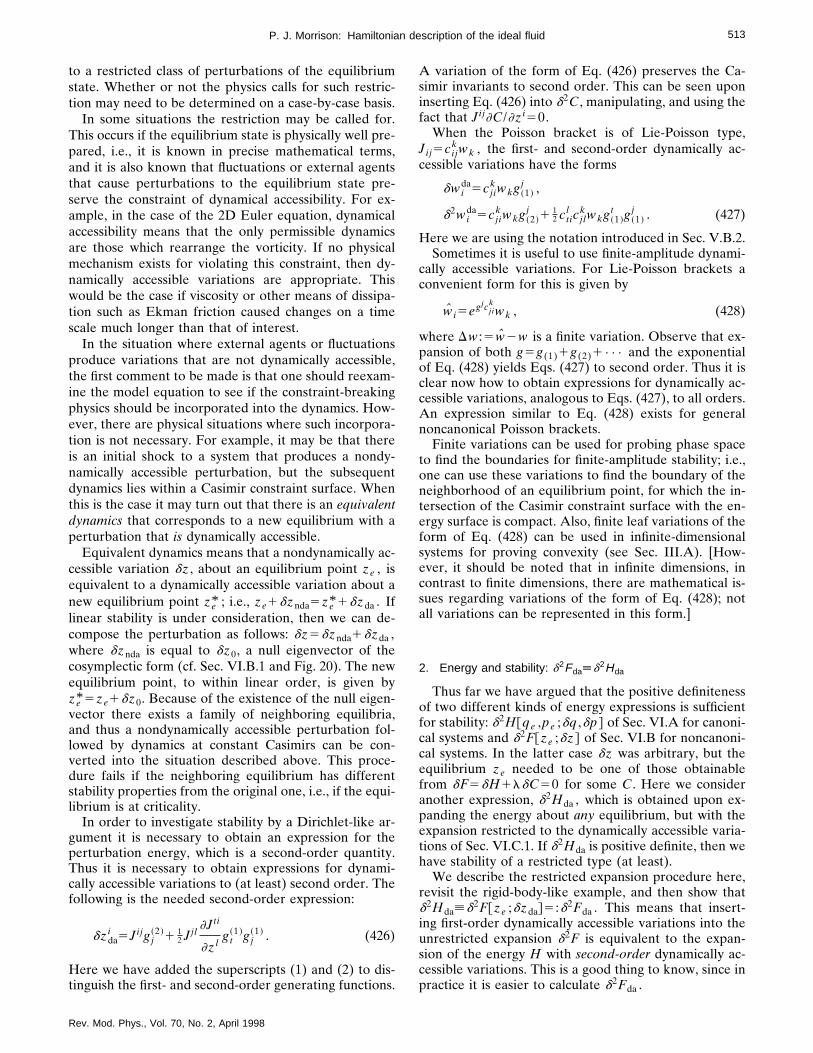
513P. J. Morrison: Hamiltonian description of the ideal fluid
to a restricted class of perturbations of the equilibriumstate. Whether or not the physics calls for such restric-tion may need to be determined on a case-by-case basis.
In some situations the restriction may be called for.This occurs if the equilibrium state is physically well pre-pared, i.e., it is known in precise mathematical terms,and it is also known that fluctuations or external agentsthat cause perturbations to the equilibrium state pre-serve the constraint of dynamical accessibility. For ex-ample, in the case of the 2D Euler equation, dynamicalaccessibility means that the only permissible dynamicsare those which rearrange the vorticity. If no physicalmechanism exists for violating this constraint, then dy-namically accessible variations are appropriate. Thiswould be the case if viscosity or other means of dissipa-tion such as Ekman friction caused changes on a timescale much longer than that of interest.
In the situation where external agents or fluctuationsproduce variations that are not dynamically accessible,the first comment to be made is that one should reexam-ine the model equation to see if the constraint-breakingphysics should be incorporated into the dynamics. How-ever, there are physical situations where such incorpora-tion is not necessary. For example, it may be that thereis an initial shock to a system that produces a nondy-namically accessible perturbation, but the subsequentdynamics lies within a Casimir constraint surface. Whenthis is the case it may turn out that there is an equivalentdynamics that corresponds to a new equilibrium with aperturbation that is dynamically accessible.
Equivalent dynamics means that a nondynamically ac-cessible variation dz , about an equilibrium point ze , isequivalent to a dynamically accessible variation about anew equilibrium point ze* ; i.e., ze1dznda5ze* 1dzda . Iflinear stability is under consideration, then we can de-compose the perturbation as follows: dz5dznda1dzda ,where dznda is equal to dz0, a null eigenvector of thecosymplectic form (cf. Sec. VI.B.1 and Fig. 20). The newequilibrium point, to within linear order, is given byze* 5ze1dz0. Because of the existence of the null eigen-vector there exists a family of neighboring equilibria,and thus a nondynamically accessible perturbation fol-lowed by dynamics at constant Casimirs can be con-verted into the situation described above. This proce-dure fails if the neighboring equilibrium has differentstability properties from the original one, i.e., if the equi-librium is at criticality.
In order to investigate stability by a Dirichlet-like ar-gument it is necessary to obtain an expression for theperturbation energy, which is a second-order quantity.Thus it is necessary to obtain expressions for dynami-cally accessible variations to (at least) second order. Thefollowing is the needed second-order expression:
dzdai 5Jijgj
~2 !1 12 Jjl
]Jti
]zlgt
~1 !gj~1 ! . (426)
Here we have added the superscripts (1) and (2) to dis-tinguish the first- and second-order generating functions.
Rev. Mod. Phys., Vol. 70, No. 2, April 1998
A variation of the form of Eq. (426) preserves the Ca-simir invariants to second order. This can be seen uponinserting Eq. (426) into d2C , manipulating, and using thefact that Jij]C/]zi50.
When the Poisson bracket is of Lie-Poisson type,Jij5cij
k wk , the first- and second-order dynamically ac-cessible variations have the forms
dwida5cji
k wkg ~1 !j ,
d2wida5cji
k wkg ~2 !j 1 1
2 ctil c jl
k wkg ~1 !t g ~1 !
j . (427)
Here we are using the notation introduced in Sec. V.B.2.Sometimes it is useful to use finite-amplitude dynami-
cally accessible variations. For Lie-Poisson brackets aconvenient form for this is given by
wi5egjcjikwk , (428)
where Dw :5w2w is a finite variation. Observe that ex-pansion of both g5g(1)1g(2)1••• and the exponentialof Eq. (428) yields Eqs. (427) to second order. Thus it isclear now how to obtain expressions for dynamically ac-cessible variations, analogous to Eqs. (427), to all orders.An expression similar to Eq. (428) exists for generalnoncanonical Poisson brackets.
Finite variations can be used for probing phase spaceto find the boundaries for finite-amplitude stability; i.e.,one can use these variations to find the boundary of theneighborhood of an equilibrium point, for which the in-tersection of the Casimir constraint surface with the en-ergy surface is compact. Also, finite leaf variations of theform of Eq. (428) can be used in infinite-dimensionalsystems for proving convexity (see Sec. III.A). [How-ever, it should be noted that in infinite dimensions, incontrast to finite dimensions, there are mathematical is-sues regarding variations of the form of Eq. (428); notall variations can be represented in this form.]
2. Energy and stability: d2Fda[d2Hda
Thus far we have argued that the positive definitenessof two different kinds of energy expressions is sufficientfor stability: d2H@qe ,pe ;dq ,dp# of Sec. VI.A for canoni-cal systems and d2F@ze ;dz# of Sec. VI.B for noncanoni-cal systems. In the latter case dz was arbitrary, but theequilibrium ze needed to be one of those obtainablefrom dF5dH1ldC50 for some C . Here we consideranother expression, d2Hda , which is obtained upon ex-panding the energy about any equilibrium, but with theexpansion restricted to the dynamically accessible varia-tions of Sec. VI.C.1. If d2Hda is positive definite, then wehave stability of a restricted type (at least).
We describe the restricted expansion procedure here,revisit the rigid-body-like example, and then show thatd2Hda[d2F@ze ;dzda#5 :d2Fda . This means that insert-ing first-order dynamically accessible variations into theunrestricted expansion d2F is equivalent to the expan-sion of the energy H with second-order dynamically ac-cessible variations. This is a good thing to know, since inpractice it is easier to calculate d2Fda .

514 P. J. Morrison: Hamiltonian description of the ideal fluid
Expanding H through second order and then restrict-ing the variations to be dynamically accessible yields
D2Hda :5]H
]zidzda
i 1]H
]zid2zda
i 112
]2H
]zi]zjdzda
i dzdaj .
(429)
Inserting Eqs. (420) and (426) into Eq. (429), observingthat the first term of Eq. (429) vanishes when evaluatedon the equilibrium, and likewise for those terms involv-ing g(2), results in
d2Hda512
]2H
]zi]zjJe
ligl~1 !Je
kjgk~1 !1
12
]H
]zi
]Jeti
]zel
Jejlgt
~1 !gj~1 ! .
(430)
Equation (430) represents the energy content of a dy-namically accessible perturbation. If this quantity ispositive definite for all g(1), then the system is stableagainst this type of perturbation.
Let us now proceed to the task of showing thatd2Hda[d2Fda . Decomposing a general first-order varia-tion as
dz5dzda1dznda (431)
and inserting into d2F yields
d2F5d2Fda1d2Fnda , (432)
where
d2Fda512S ]2H~ze!
]zi]zj1la
]2Ca~ze!
]zi]zj D3Jli~ze!gl
~1 !Jkj~ze!gk~1 ! . (433)
It is always the case that d2F da depends only on thefirst-order g’s.
We note that d2F can be indefinite because of thepresence of d2Fnda , even if d2Fda , which involves onlyvariations of the form Jij(ze)gi
(1) , is of definite sign. Anexample is given by the free-rigid-body-like system withthe equilibrium
l 1e52
BI1
lI111, l 2
e5l 3e50, (434)
where we set B15B and B25B350. In this case
d2F52B
2l 1e ~dl 1!21
12S 1
I22
1I1
D ~dl 2!2
112S 1
I32
1I1
D ~dl 3!2. (435)
If I1,I2,I3, the last two terms are positive; however,the first term can have either sign. Dynamically acces-sible variations satisfy
dl ida5e ijkl j
egk5e ijkl jegk ; (436)
hence dl 1da50. Therefore d2Fda is definite, even though
d2F need not be.45 Observe, also, that the nondynami-cally accessible variation corresponds to the null eigen-vector described above.
Rev. Mod. Phys., Vol. 70, No. 2, April 1998
To see that in general d2Fda is identical to d2Hda , weexpand some Casimir Ca to second order about theequilibrium:
D2Ca5]Ca
]zidzi1
]Ca
]zid2zi1
12
]2Ca
]zi]zjdzidzj, (437)
which when restricted to the constraint surface reducesto
D2Cdaa 5
]Ca
]ziJe
ligl~1 !1
]Ca
]ziJe
ligl~2 !
112
]Ca
]zi
]Jeti
]z0l
Jejlgt
~1 !gj~1 !
112
]2Ca
]zi]zjJe
ligl~1 !Je
kjgk~1 ! . (438)
The first and second terms in Eq. (438) clearly vanishbecause of
Jij]Ca
]zj50. (439)
By the definition of dynamical accessibility, the last twoterms must cancel; thus, to second order D2Cda
a vanishesidentically. Indeed, one can realize Eq. (439) as a Taylorseries about the equilibrium point ze and observe that,since this equation holds for all z (at least in a neighbor-hood of ze), each power of dz in the expansion
05Jij]Ca
]zj(440)
5Jeij ]Ca
]zej
1dzlS ]Jeij
]zel
]Ca
]zej
1Jeij ]2Ca
]zel ]ze
j D 1•••
must vanish identically. The first term in Eq. (440) isclearly zero, while the vanishing of the second term, theone linear in dzl, yields a desired relation
]Jeij
]zel
]Ca
]zej
52Jeij ]2Ca
]zel ]ze
j, (441)
between the first and second partial derivatives of Ca. Inthis way it follows immediately that D2Cda[0.
It is evident that the first term of Eq. (430) is the sameas the first term of the free energy d2Fda of Eq. (433),but in order to compare the second terms in these equa-tions, one must use Eq. (441) and the equilibrium con-dition (398) involving the Lagrange multipliers. Indeed,by summing Eq. (441) over la and then exploiting Eq.(398), we conclude that
45It is important to keep in mind that the existence of anindefinite conserved quadratic form does not imply instability.Dirichlet-like theorems give only a sufficient condition for sta-bility; negative-energy modes provide the counterexample thatprecludes necessity (cf. Sec. VI.A).

515P. J. Morrison: Hamiltonian description of the ideal fluid
laJeij ]2Ca
]zel ]ze
j52la
]Jeij
]zel
]Ca
]zej
5]Je
ij
]zel
]H
]zej
. (442)
It thus follows, as was asserted, that d2Hda[d2Fda .Note that although the two energy expressions are
equivalent, the derivation of the d2Fda is valid only forthose equilibria that are extremal points of F5H1lCfor some C , while d2Hda has no such restriction.
3. Dynamically accessible fluid energy: d2Hda
By now it should be clear that there exist three differ-ent kinds of energy expressions: d2H , d2F , and d2Hda .The expression d2H@qe ,pe ;dq ,dp# occurs in the canoni-cal description and lives on the largest phase space, theexpression d2F@we ;dw# occurs in the noncanonical de-scription and lives on the reduced phase space, and theexpression d2Hda@we ;g# occurs in the noncanonical de-scription and, because it is constrained to symplecticleaves which are subsurfaces of the reduced phase space,lives on the smallest phase space. Below we computed2Hda for the general 3D compressible fluid. To this endwe construct first- and second-order dynamically acces-sible variations, show how such first-order variationsgive rise to all fluid equilibria as extremals of the energy,calculate the second variations of the potential and ki-netic energies, and thus obtain d2Hda . Lastly, we com-pare d2Hda with d2H , the Lagrangian variable expres-sion for the second-order fluid energy as calculated inSec. VI.A.2, and briefly comment on its utility.
a. Dynamically accessible variations
To obtain dynamically accessible variations for thefluid, the functional
G:5ED
~M•h1hr1ks!d3r (443)
can be inserted into the bracket of Eq. (209). Here thearbitrariness of variation within the symplectic leaf isdescribed by the functions of h , h , and k , which are freefunctions of position. Following are expressions for thefirst-order variations of the momentum density, massdensity, and entropy per unit mass, respectively:
dMda5$G,M%5@M ,h#†1r¹h1s¹k ,
drda5$G,r%5¹•S rdGdM D5¹•~rh!,
dsda5$G,s%5¹•S sdGdM D5¹•~sh!. (444)
Recall that @M ,h# i† :5M•] ih1¹•(Mih), where
] i :5]/]xi, satisfies the identities ^M ,@f ,g#&5^@M ,g#†,f#&52^@M ,f#†,g#&, where @ , # is defined byEq. (355). These identities require that one of M•n , f•n ,and g•n vanish on the boundary, where we recall that nis a vector normal to the boundary. We assumeMe•n[0 and h•n[0, and thus drda and dsda do notchange the total mass and entropy.
Rev. Mod. Phys., Vol. 70, No. 2, April 1998
Observe that the variations drda and dsda of Eq. (444)are identical to dr and ds of Eq. (323) if we make theidentification dq5j(a ,t)5h(r ,t). Therefore, for thesequantities, first-order dynamically accessible variationsare precisely the same as Eulerian variations induced byunderlying Lagrangian variable variations. Also, uponidentifying M5p/J and comparing dM of Eq. (323)with dMda of Eq. (444), we obtain
dp i52p•] ih2r0] ih2s0] ik , (445)
i.e., if dp satisfies Eq. (445), then the dM obtained fromEq. (323) will be dynamically accessible. Because dp isarbitrary on the Lagrangian level, not all Lagrangianvariations will be of the form of Eq. (445), and thus notall induced Eulerian variations will be dynamically ac-cessible.
In order to calculate the energy expression, we needthe following expressions for dynamically accessiblevariations to second order:
d2Mdai512 $G,ˆG,M%‰i
5 12 $†@M ,h#†,h‡i
†1¹•~rh!] ih
1¹•~rh] ih !1r~] jh !~] ih j!
1¹•~sh!] ik1¹•~sh] ik !
1s~] jk !~] ih j!%,
d2rda512 ˆG,$G,r%‰5 1
2 ¹•@h¹•~rh!# ,
d2sda512 ˆG,$G,s%‰5 1
2 ¹•@h¹•~sh!# . (446)
These second-order variations should include depen-dence upon second-order generating functions as in Sec.VI.C.1, but the second-order pieces do not contributebelow, so we neglect them.
b. Equilibria
Now we show how all 3D fluid equilibria are gottenfrom the vanishing of the first-order dynamically acces-sible variation of the fluid energy,
H@r ,s ,M#5EDS M2
2r1rU~r ,s! Dd3r , (447)
where we recall that U(r ,s) is the internal energy perunit mass. Here we have used the tilde to indicate thatthe dependence is upon r and s instead of r and s . Interms of U(r ,s) the equation of state for the pressure isgiven by
p ~r ,s!5r2S ]U
]r1
s
r
]U
]sD . (448)
The first variation of H is
dH5EDFM
r•dM2
M2
2r2dr1drS U1r
]U
]rD
1dsS r]U
]sD Gd3r . (449)

516 P. J. Morrison: Hamiltonian description of the ideal fluid
Inserting Eq. (444), integrating by parts, and usingM5rv yields
dHda@h ,h ,k#5ED
~h j@2M•] jv2] i~rv iv j!
1r] j~v2/2!2r] j~U1rUr!
2s] j~rUs!#2h@¹•M#
2k@¹•~sM/r!#!d3r . (450)
Since h , h , and k are arbitrary, dHda[0 implies that the@ . . . # terms of Eq. (450) vanish individually. These areeasily shown to imply the usual Eulerian equilibriumequations for a compressible fluid:
] j~rv iv j!1] ip50,
] j~rv j!50,
v j] js50. (451)
c. Potential energy
Now consider the expansion of the potential-energyfunctional,
W@r ,s#5ED
rU~r ,s!d3r , (452)
to second order. Upon Taylor expansion, we obtain
d2W5 12 E
D@~dr!2~rUrr12Ur!1~ds!2~rUss!
12~dsdr!~rUrs1Us!12~d2r!~rUr1U !
12~d2s!~rUs!#d3r , (453)
where subscripts denote partial differentiation. InsertingEq. (444) and (446) into Eq. (453) creates a relativelycomplicated formula, one with several terms that looksimilar, but simplification is not obvious. What we haveis a sort of integration-by-parts puzzle. We shall not giveall the details here of a calculation that gets us to thedesired end, but only a few ‘‘moves’’ and ‘‘landmarks.’’The first move is to integrate the second-order varia-tions by parts. Next, the terms are grouped as follows:
d2Wda@h#5 12 E
D@~¹•h!2~r3Urr12r2Ur1s2rUss
12sr2Usr12srUs!
1~¹•h!~h•¹s!~srUss1r2Urs1rUr!
1~¹•h!~h•¹r!~r2Urr12rUr
1srUrs1sUs!#d3r , (454)
which upon making use of Eq. (448) can be put into theform
Rev. Mod. Phys., Vol. 70, No. 2, April 1998
d2Wda@h#5 12 E
D@~¹•h!2~r p r1s p s!
1~¹•h!~h•¹ p !#d3r . (455)
The definition p(r ,s):5 p(r ,s) and the chain rule implyr p r1s p s5rpr , which when used in Eq. (455) yields,finally,
d2Wda@h#5 12 E
D@~¹•h!2~rpr!1~¹•h!~h•¹p !#d3r .
(456)
This expression, when evaluated on r5re and s5se , isprecisely that calculated in the footnote following Eq.(384), which was obtained in the strictly Lagrangianvariable context. This is to be expected, since the dy-namically accessible variations of density and entropyare the same as those induced by Lagrangian variations.
d. Kinetic energy
Now consider the expansion of the kinetic-energyfunctional,
T@r ,M#5ED
M2
2rd3r , (457)
to second order. Upon Taylor expansion, we obtain
d2T5EDFM
r•d2M2
M2
2r2d2r1
M2
2r3~dr!2
2drM
r2•dM1
~dM !2
2r Gd3r . (458)
We shall reduce this expression to a familiar form bysolving another integration-by-parts puzzle. Making useof dM5rdv1vdr , which is a valid identity whether ornot the variations dr and dM are dynamicallyaccessible,46 yields the simplified expression
d2T5EDFv•d2M2
v2
2d2r1
r
2~dv !2Gd3r . (459)
Now restricting ourselves to dynamically accessiblevariations by inserting Eqs. (444) and (446) into Eq.(459) yields
46Using Eq. (444) yields dvdai5v•] ih1h•¹v i1] ih1s] ik ,which is different from the expression for dv in terms of thedisplacement: dv5h1v•¹h2h•¹v .

517P. J. Morrison: Hamiltonian description of the ideal fluid
d2Tda@h ,h ,k#512ED
H v•†@M ,h#†‡
†1¹•~rh!~v•¹h !
1v i¹•~rh] ih !1r~v•¹h i!~] ih !
1¹•~sh!~v•¹k !1v i¹•~sh] ik !
1s~v•¹h i!~] ik !2v2
2¹•@h¹•~rh!#
1r~dvda!2J d3r . (460)
Making use of the identity ^@x ,g#†,f&5^x ,@f ,g#&, effect-ing some cancellation, and rearranging, gives
d2Tda@h ,h ,k#512ED
@rdvda•~@v ,h#1dvda!
1drda@v•¹h1v•~v•¹h!#
1dsda~v•¹k !#d3r . (461)
Introducing
Pi :5rv•] ih1r] ih1s] ik , (462)
which satisfies rdvda5rh•¹v1P , we obtain from Eq.(461)
d2Tda@h ,h ,k#512ED
FP2
r1Pi~v•¹h i1h•¹v i!
1r~h•¹v i!~v•¹h i!
1drda@v•¹h1v•~v•¹h!#
1dsda~v•¹k !Gd3r . (463)
After several integrations by parts and making use ofthe equilibrium relations of Eq. (451), we obtain ourdesired result,
d2Tda@h ,h ,k#512ED
FP2
r12P•~v•¹h!
2~h•¹h!•¹p Gd3r . (464)
e. Total energy
Adding Eqs. (456) and (464) gives the following ex-pression for the total, dynamically accessible energy of aperturbation to an Eulerian equilibrium state:
d2Hda@h ,h ,k#512ED
FP2
re12P•~ve•¹h!
1~¹•h!2~reper!1~¹•h!~h•¹pe!
2~h•¹h!•¹peGd3r . (465)
It is interesting to compare the energy d2Hda of Eq.(465) with its counterpart d2H of Eq. (393), which wasderived within the Lagrangian variable context. If we
Rev. Mod. Phys., Vol. 70, No. 2, April 1998
observe that Pi[2dp i /J, where dp i is given by Eq.(445), and identify P with 2ph , then these energy ex-pressions are identified. However, as noted above thereis a difference in that ph at fixed h is completely arbi-trary in the Lagrangian variable context, while the free-dom of P at fixed h is constrained to be determined byEq. (462), which contains only the two free functions hand k .
The energy expression d2Hda can be rewritten inmany different ways by integration by parts and by mak-ing use of the equilibrium equations (451). We shall notpursue this further here, but it is clear how to obtainDirichlet-like stability criteria: if for some equilibriumd2Hda@h ,h ,k# can be manipulated into a positive defi-nite form, then we have stability against dynamically ac-cessible perturbations. One can proceed with d2Hda in amanner similar to that used in MHD analyses of thestability of plasma devices (see, for example, Newcomb,1960; Hazeltine and Meiss, 1992), where minimizationsare carried out in order to ascertain whether or not theenergy functional is positive definite.47
The sufficient conditions for stability that result fromthe procedure described above are equivalent to Ray-leigh or Fjortoft-type criteria, which are usually stated asnecessary conditions for instability. Criteria such as theRayleigh inflection point criterion for fluid shear floware in essence conditions for the positive definiteness ofthe energy. This explains why similar criteria occur in avariety of fluid and plasma contexts. The expressiond2Hda is a quite general starting point for doing this kindof stability analysis for a wide variety of equilibria anddynamics.
VII. CONCLUSION
One thing that is clear from the above section, indeedfrom this entire article, is that there are many differentways of writing the equations that describe fluid phe-nomena. These different ways amount to the choice ofvariables employed, such as Lagrangian, Eulerian, orClebsch, and the different variables give rise to the dif-ferent kinds of Hamiltonian structure. Although one canargue that underlying it all is Newton’s second law to-gether with constraints, such as mass conservation or theconstancy of entropy, the different ways of describing afluid imply different phrasings of the constraints. Thisdifference in phrasing gives rise to differences in theusual analyses of fluid phenomena, notably stabilityanalyses. Generally speaking, when two things are dif-ferent, each has advantages. In closing we explore thisand related stability issues a bit.
One consequence of phrasing the constraints in differ-ent ways is the occurrence of the different kinds of en-ergy expressions that we have described. The use of d2Ffor obtaining stability criteria, the energy-Casimirmethod, is relatively simple, direct, and extendable to
47Sun and Finn (1987), Pfirsch (1990), and Isichenko (1997)have done calculations of this sort for MHD.

518 P. J. Morrison: Hamiltonian description of the ideal fluid
nonlinear stability analysis, but is limited to a restrictedclass of equilibrium states, viz., those that arise as extre-mals of F5H1lC . However, the use of d2Hda has nosuch restriction and it can be calculated for all equilibria,but this approach has difficulties that need to be over-come in a rigorous mathematical analysis.48
A consequence of the above is that the restricted classof equilibria obtained by extremizing F5H1lC issingled out. Thus it is natural to ask, is there somethingspecial about these equilibria? One thing for certain isthat this class includes the dynamical equilibrium statethat corresponds to thermodynamic equilibrium. For ex-ample, for the 3D compressible fluid, the equilibriumequations (396) yield the state of thermodynamic equi-librium corresponding to zero mean flow and uniformdensity. In fact the condition dF50, in the case wherev50, can be made to be identical to the thermodynamicminimum-energy principle (Callen, 1960), and d2F posi-tive definite corresponds in this case to thermodynamicstability (Le Chatelier’s principle). Similarly for Vlasovtheory, dF50 can be made to yield the Maxwellianphase-space density. Generally speaking it appears thatthese special equilibria are more likely to be stable thanother equilibria, and proofs of nonlinear stability forthem are possible in many cases. Indeed for both the 2DEuler equation and for Vlasov theory the restricted classcorresponds to equilibria where the vorticity and phase-space density are monotonic functions of the streamfunction and energy, respectively. These equilibria donot have negative-energy modes (NEMs).
Any of the various energy expressions can be used todetermine the existence of NEMs, but additional infor-mation is required. In particular, if it is known by somemeans that the system is spectrally stable and that theenergy functional, whichever type, is not positive defi-nite, then the system can have a NEM. By definition, ifthe eigenfunction of a NEM is substituted into the en-ergy functional, then one obtains a negative expression.Similarly, if the eigenfunction of a positive-energy modeis substituted, then one obtains a positive expression. Inboth these cases mode means a stable pure oscillation—the energy associated with an unstable eigenfunctionnecessarily is zero. Thus associated with an eigenfunc-tion is a signature.
Signature is important in that it gives an indication ofpossible behavior, as illustrated by the examples of Secs.VI.A and VI.A.1. From many examples, both finite andinfinite, one can infer a general two-part principle re-garding systems with NEMs (see, for example, Morrisonand Kotschenreuther, 1990): (i) ideal stable systems withboth positive- and negative-energy modes tend to benonlinearly unstable, and (ii) if an ideal system with a
48Namely, to attempt a nonlinear dynamically accessible sta-bility analysis one must define the class of functions that arerepresentable by the exponential of Sec. VI.C.1, and this isdifficult. Also, this class of functions is not closed under theusual operations, and so the taking of limits is difficult to de-fine (see, for example, de la Llave, 1993).
Rev. Mod. Phys., Vol. 70, No. 2, April 1998
NEM is perturbed by adding terms to the dynamicalsystem that extract energy, then a NEM (which by defi-nition is neutrally stable) becomes unstable. This prin-ciple is clearly not a theorem: additional invariants canpreclude the existence of nonlinear instability, and onemust be sure that the dissipation actually extracts energyfrom a NEM in order for it to be destabilized.
Systems with symmetry possess other invariants, con-stants of motion that commute with the particularHamiltonian (unlike Casimir invariants, which commutewith all Hamiltonians). Extremization of the energy withthese constants held fixed, which can be achieved by us-ing Lagrange multipliers, yields relative equilibria, i.e.,equilibria in frames of reference generated by the invari-ants. For example, extremization of H1l•P , where P isthe momentum, gives a state that is uniformly translat-ing at the velocity l. Alternatively, one can interpret theextremal points obtained from extremizing the Hamil-tonian at fixed invariants as being the equilibrium ofinterest observed in a different frame of reference. Ifthere exists any frame of reference in which the energyfunctional is definite, then both linear and, for finite sys-tems, nonlinear instability are precluded. Further, onecan analyze the energy with the variations restricted tolie within the surfaces defined by the invariants, in amanner similar to that used in Sec. VI.C where dynami-cal accessibility was discussed.49 In general, if any com-bination of known invariants implies the existence of afamily of compact invariant sets about an equilibrium,then from the definition of Sec. VI.A that equilibrium isnonlinearly stable.
The existence of different frames of reference also af-fects the second part of our two-part principle becausedissipation is frame dependent. This is easily demon-strated by an example due to Poincare (1885). Considera particle subjected to gravity and confined within aclear, spherical, rotating bowl. Clearly the point at thebottom of the bowl is an equilibrium point in any frameof reference. If there is no friction between the particleand the bowl, then the particle will oscillate about thebottom point, whether or not the bowl is rotating. How-ever, if friction is added (by, for example, applying hair-spray), then a stationary observer who is unable to dis-cern the bowl, will see a strange effect of the‘‘dissipation.’’ Rather than seeing the friction damp theoscillation, the stationary observer will see the particleleave the vicinity of the bottom equilibrium point as itgrabs onto the side of the bowl. Clearly care must takenwhen defining dissipation, since in this example the sta-tionary observer sees energy being put into the particle,while a rotating observer sees the particle attempting tocome to rest with the rotating bowl.
The energy-Casimir (Arnold’s) method or any energymethod for obtaining sufficient conditions for stabilityprovides an incomplete analysis of a problem. It is in-complete because the indefiniteness of the energy func-
49See, for example, Ilgisonis and Pastukhov (1996) and Ilgiso-nis (1996) for a recent use of this idea in the context of MHD.

519P. J. Morrison: Hamiltonian description of the ideal fluid
tional implies either the existence of NEMs or instabil-ity, and, as noted above, there is no way in general ofdistinguishing from any of the energy expressions alonewhich is the case. More importantly, it is incomplete be-cause stability is not the whole issue: a complete analysiswould determine the dynamics given an initial condition.Thus to finish the linear problem one must find a com-plete set of eigenfunctions; i.e., a normal-mode analysismust be done.
This normal-mode analysis is rather difficult becauseusually fluid and plasma systems possess continuouseigenspectra, unlike the complete discrete spectrum thatoccurs in elementary quantum mechanics problems. Inthe Hamiltonian setting, finishing the linear problemamounts to finding a transformation to action angle vari-ables, variables that are related to the eigenfunctions ofthe continuous spectrum. For systems that are nonca-nonical this transformation has two parts: canonizingand diagonalizing. One must find a set of canonical vari-ables on the symplectic leaf and then one must find thecanonical transformation that diagonalizes the Hamil-tonian. This program has been carried out for the Vla-sov system (Morrison and Pfirsch, 1992; Morrison andShadwick, 1994) using Van Kampen singular eigenfunc-tions (see, for example, Van Kampen and Felderhoff,1967). The necessary mathematical tools have been gen-eralized (Balmforth and Morrison, 1995) and applied toinviscid shear flow with a broad class of fluid equilibriumflow profiles. This is a long story, one that will be re-ported elsewhere (Balmforth and Morrison, 1998).
ACKNOWLEDGMENTS
A. N. Kaufman, R. Salmon, and R. D. Hazeltine en-couraged me to complete this article. A. N. Kaufman, R.Salmon, and T. Shepherd made extensive comments andcorrections on an earlier version. Notes from the Geo-physical Fluid Dynamics Summer School, on which thisarticle is based, were prepared with the help of the fel-lows: O. Buhler, D. del-Castillo-Negrete, G. Dairiki, S.McNamara, K. Ngan, C. Nore, D. Petrich, K. Swanson,and R. Worthing. B. Shadwick helped with the figures,aided with TEX, and made comments on the text. Ad-ditional comments and corrections were made by N. J.Balmforth, O. Bokhove, R. de la Llave, R. Ford, N.Padhye, G. Tarkenton, L. C. Morrison, G. Rein, E. Spie-gel, J.-L. Thiffeault, J. Vanneste, T. Warn, T. Yudichak,and others. The content of the article was influenced bymany, including my collaborators J. M. Greene, J. Mars-den, D. Pfirsch, and (the late) W. B. Thompson. To all ofthe above and to those I have neglected to mention, Iam most grateful. The hospitality of the Woods HoleOceanographic Institution, where the original lectureswere given, and of the Isaac Newton Insitute of Cam-bridge University, where a portion of the article was ed-ited, are gladly acknowledged, along with the support ofthe U.S. Department of Energy under contract No. DE-FG05-80ET-53088.
Rev. Mod. Phys., Vol. 70, No. 2, April 1998
REFERENCES
Arnold, V. I., 1963, Usp. Mat. Nauk [Sov. Math. Usp.] 18, 85.Arnold, V. I., 1966a, Izv. Vyssh. Uchebn. Zaved. Mat. [Sov.
Math. J.] 5, 3.Arnold, V. I., 1966b, Ann. Inst. Fourier 16, 319.Arnold, V. I. 1969, Usp. Mat. Nauk. [Sov. Math. Usp.] 24, 225.Arnold, V. I., 1978, Mathematical Methods of Classical Me-
chanics (Springer, Berlin).Arnold, V. I., V. V. Kozlov, and A. I. Neishtadt, 1990, Dynam-
ics III: Mathematical Aspects of Classical and Celestial Me-chanics (Springer, Berlin).
Balmforth, N. J., and P. J. Morrison, 1995 (Institute for FusionStudies, University of Texas, Austin), Report No. 692. SeeNational Technical Information Service Document No.DE95008952INZ. Copies may be obtained from NTIS, 5285Port Royal Rd., Springfield, VA 22161, http://www.ntis.gov.
Balmforth, N. J., and P. J. Morrison, 1998, Mathematics of At-mosphere and Ocean Dynamics, Proceedings of the IsaacNewton Institute Program, edited by I. Roulstone and J. Nor-burg (Cambrige University, Cambridge), in press.
Bartholomew, P., 1971, Mon. Not. R. Astron. Soc. 151, 333.Bernstein, I., 1958, Phys. Rev. 109, 10.Bernstein, I., E. A. Frieman, M. D. Kruskal, and R. M.
Kulsrud, 1958, Proc. R. Soc. London, Ser. A 244, 17.Berry, M. V., 1978, in Topics in Nonlinear Dynamics, AIP
Conference Proceedings No. 46, edited by S. Jorna (AIP,New York), p. 16.
Bialynicki-Birula, I., and P. J. Morrison, 1991, Phys. Lett. A158, 453.
Birkhoff, G. D., 1927, Dynamical Systems (American Math-ematical Society, New York).
Bretherton, F. P., 1970, J. Fluid Mech. 44, 19.Cairns, R. A., 1979, J. Fluid Mech. 92, 1.Calkin, M., 1963, Can. J. Phys. 41, 2241.Callen, H. B., 1960, Thermodynamics (Wiley, New York).Cherry, T. M., 1925, Trans. Cambridge Philos. Soc. 23, 199.Clebsch, A., 1857, J. Reine Angew. Math. 56, 1.Courant, R., and D. Hilbert, 1953, Methods of Mathematical
Physics (Wiley Interscience, New York).Clebsch, A., 1859, J. Reine Angew. Math. 54, 293.de la Llave, R., 1993, in Proceedings II Granada Seminar in
Computational Physics, edited by P. L. Garrido and J. Marro(World Scientific, Singapore), pp. 73–106.
del-Castillo-Negrete, D., J. M. Greene, and P. J. Morrison,1997, Physica D 100, 311.
del-Castillo-Negrete, D., and P. J. Morrison, 1993, Phys. FluidsA 5, 948.
Dirichlet, P. G. L., 1846, Crelle 32, 3.Dubrovin, B. A., and S. P. Novikov, 1984, Sov. Math. Dokl. 30,
651.Dzyaloshinskii, I. E. and G. E. Volovick, 1980, Ann. Phys.
(N.Y.) 125, 67.Eckart, C., 1960, Phys. Fluids 3, 421.Eisenhart, L. P., 1961, Continuous Groups of Transformations
(Dover, New York).Falcolini, C., and R. de la Llave, 1992, J. Stat. Phys. 67, 609.Filippov, D. V., and V. V. Yan’kov, 1986, Sov. J. Plasma Phys.
12, 548.Fjortoft, R., 1950, Geofys. Publ. 17, 1.Fowler, K., 1963, J. Math. Phys. 4, 559.Frieman, E., and M. Rotenberg, 1960, Rev. Mod. Phys. 32, 898.Gardner, C. S., 1963, Phys. Fluids 6, 839.
520 P. J. Morrison: Hamiltonian description of the ideal fluid
Gardner, C. S., 1971, J. Math. Phys. 12, 1548.Gelfand, I. M. and S. V. Fomin, 1963, Calculus of Variations
(Prentice-Hall, Englewood Cliffs, NJ).Greene, J. M., 1979, J. Math. Phys. 20, 1183.Greene, J. M., and B. Coppi, 1965, Phys. Fluids 8, 1745.Greenspan, H. P., 1968, Theory of Rotating Fluids (Cambridge
University, Cambridge, England).Gursey, F., 1963, in Relativity, Groups and Topology, edited by
C. DeWitt and B. DeWitt (Gordon Breach, New York), p. 91.Hain, V. K., R. Lust, and A. Schluter, 1957, Z. Naturforsch.
Teil A 12, 833.Hammermesh, M., 1962, Group Theory and its Applications to
Physical Problems (Addison-Wesley, Reading, MA).Hazeltine, R. D., and J. D. Meiss, 1992, Plasma Confinement
(Addison-Wesley, Redwood City, CA).Holm, D. D., and B. Kupershmidt, 1983, Physica D 6, 347.Holm, D. D., J. E. Marsden, T. Ratiu, and A. Weinstein, 1985,
Phys. Rep. 123, 1.Ilgisonis, V. I., 1996, Phys. Plasmas 3, 4577.Ilgisonis, V. I., and V. P. Pastukhov, 1996, Plasma Phys. Rep.
22, 209.Isichenko, M., 1997, private communication.Jacobson, N., 1962, Lie Algebras (Wiley Interscience, New
York).Kandrup, H. E., and P. J. Morrison, 1993, Ann. Phys. (N.Y.)
225, 114.Kreın, M. G., and V. A. Jakubovic, 1980, Four Papers on Or-
dinary Differential Equations (American Mathematical Soci-ety, Providence, Rhode Island).
Kruskal, M. D., and C. Oberman, 1958, Phys. Fluids 1, 275.Kueny, C., Ph.D. thesis, The University of Texas at Austin,
Austin, Texas, 1993.Kueny, C. S., and P. J. Morrison, P. J., 1995a, Phys. Plasmas 2,
1926.Kueny, C. S., and P. J. Morrison, 1995b, Phys. Plasmas 2, 4149.Kuznetsov, E. A., and A. Mikhailov, 1980, Phys. Lett. A 77, 37.Lagrange, J. L., 1788, Mecanique Analytique (Desaint, Paris).Lamb, H., 1945, Hydrodynamics (Dover, New York).Laval, G., C. Mercier, and R. Pellat, 1965, Nucl. Fusion 5, 156.Lax, P., 1975, Commun. Pure Appl. Math. 28, 141.Lewis, D., J. Marsden, R. Montgomery, and T. Ratiu, 1986,
Physica D 18, 391.Likins, P. W., 1971, AGARD Lecture Series 3b, 1.Littlejohn, R., 1981, private communication.Littlejohn, R., 1982, in Mathematical Methods in Hydrodynam-
ics and Integrability in Related Dynamical Systems, AIP Con-ference Proceedings No. 88, edited by M. Tabor and Y. Treve(AIP, New York), p. 47.
Loewner, C., 1971, Theory of Continuous Groups, notes by H.Flanders and M. Protter (MIT Press, Cambridge, MA).
MacKay, R. S., 1982, Ph.D. thesis (Princeton University).MacKay, R. S., and P. G. Saffman, 1986, Proc. R. Soc. London,
Ser. A 406, 115.Magri, F., 1978, J. Math. Phys. 19, 1156.Marsden, J. E., 1993, Lectures on Mechanics (Cambridge Uni-
versity, Cambridge, England).Marsden, J. E., and P. J. Morrison, 1984, Contemp. Math. 28,
133.Marsden, J. E., and A. Weinstein, 1974, Rep. Math. Phys. 5,
121.Marsden, J. E., and A. Weinstein, 1983, Physica D 7, 305.
Rev. Mod. Phys., Vol. 70, No. 2, April 1998
Marsden, J. E., A. Weinstein, T. Ratiu, R. Schmid, and R.Spencer, 1983, in Proceedings of IUTAM-IS1MM Symposiumon Modern Developments in Analytical Mechanics, Atti dellaAccad. Sci. Torino 117, 289.
McIntyre, M. E., and T. G. Shepherd, 1987, J. Fluid Mech. 181,527.
Meacham, S. P., G. R. Flierl, and P. J. Morrison, 1997, Phys.Fluids 9, 2310.
Meiss, J. D., 1992, Rev. Mod. Phys. 64, 795.Montgomery, D., and R. Kraichnan, 1979, Rep. Prog. Phys. 43,
35.Morrison, P. J., 1980, Phys. Lett. A 80, 383.Morrison, P. J., 1981a, ‘‘Hamiltonian field description of two-
dimensional vortex fluids and guiding center plasmas,’’ Prin-ceton University Plasma Physics Laboratory Report, PPPL-1783. Available as American Institute of Physics DocumentNo. PAPS-PFBPE-04-771-24, AIP Auxiliary Publication Ser-vice, 500 Sunnyside Blvd., Woodbury, NY 11797-2999, http://www.aip.org/epaps/.
Morrison, P. J., 1981b, ‘‘Hamiltonian field description of One-Dimensional Poisson-Vlasov Equation,’’ Princeton Univer-sity Plasma Physics Laboratory Report, PPPL-1788. Avail-able as American Institute of Physics Document No. PAPS-PFBPE-04-771-14, AIP Auxiliary Publication Service, 500Sunnyside Blvd., Woodbury, NY 11797-2999, http://www.aip.org/epaps/.
Morrison, P. J., 1982, in Mathematical Methods in Hydrody-namics and Integrability in Related Dynamical Systems, AIPConference Proceedings No. 88, edited by M. Tabor and Y.Treve (AIP, New York), p. 13.
Morrison, P. J., 1987, Z. Naturforsch. 42a, 1115.Morrison, P. J., 1994, ‘‘Hamiltonian Description of the Ideal
Fluid,’’ in Geophysical Fluid Dynamics, edited by R. Salmonand B. Ewing-Deremer (Woods Hole Oceanographic Insti-tute, Woods Hole, 1994), Technical Report No. WHOI-94-12.See National Technical Information Service Document No.DE94007372INZ. Copies may be obtained from the NTIS,5285 Port Royal Rd., Springfield, VA 22161; http://www.ntis.gov.
Morrison, P. J., and S. Eliezer, 1986, Phys. Rev. A 33, 4205.Morrison, P. J., and J. M. Greene, 1980, Phys. Rev. Lett. 45,
790; 48, 569(E).Morrison, P. J., and R. D. Hazeltine, 1984, Phys. Fluids 27, 886.Morrison, P. J., and M. Kotschenreuther, 1990, in Nonlinear
World: IV International Workshop on Nonlinear and Turbu-lent Processes in Physics, edited by V. G. Bar’yakhtar, V. M.Chernousenko, N. S. Erokhin, A. B. Sitenko, and V. E. Za-kharov (World Scientific, Singapore), p. 910.
Morrison, P. J., and D. Pfirsch, 1989, Phys. Rev. A 40, 3998.Morrison, P. J., and D. Pfirsch, 1990, Phys. Fluids B 2, 1105.Morrison, P. J., and D. Pfirsch, 1992, Phys. Fluids B 4, 3038.Morrison, P. J., and B. A. Shadwick, 1994, Acta Phys. Pol. A
85, 759.Moser, J. K., 1958, Commun. Pure Appl. Math. 11, 81.Moser, J. K., 1968, Mem. Am. Math. Soc. 81, 1.Moser, J. K., 1973, Stable and Random Motions in Dynamical
Systems (Princeton University, Princeton).Nambu, Y., 1973, Phys. Rev. D 7, 2405.Newcomb, W. A., 1960, Ann. Phys. (N.Y.) 10, 232.Newcomb, W. A., 1962, Nucl. Fusion Suppl. 2, 451.Newcomb, W. A., 1967, Proc. Symp. Appl. Math. 18, 152.Nycander, J., 1992, Phys. Fluids A 4, 467.Olver, P. J., 1982, J. Math. Anal. Appl. 89, 233.

521P. J. Morrison: Hamiltonian description of the ideal fluid
Ottino, J. M., 1990, Annu. Rev. Fluid Mech. 22, 207.Padhye, N., and P. J. Morrison, 1996a, Phys. Lett. A 219, 287.Padhye, N., and P. J. Morrison, 1996b, Plasma Phys. Rep. 22,
869.Pedlosky, J., 1987, Geophysical Fluid Dynamics, 2nd edition
(Springer, New York).Pfirsch, D., 1990, private communication.Pfirsch, D., 1993, Phys. Rev. A 48, 1428.Pfirsch, D., and R. N. Sudan, 1993, Phys. Fluids B 5, 2052.Poincare, H., 1885, Acta Math. VII, 259.Ramani, A., B. Grammaticos, and T. Bountis, 1989, Phys. Rep.
180, 161.Rein, G., 1994, Math. Methods Appl. Sci. 17, 1129.Ripa, P., 1981, Nonlinear Properties of Internal Waves, AIP
Conference Proceedings No. 76, edited by B. J. West (AIP,New York), p. 281.
Ripa, P., 1993, Geophys. Astrophys. Fluid Dyn. 70, 85.Saletan, E., and A. Cromer, 1971, Theoretical Mechanics
(Wiley, New York).Salmon, R., 1982, in Mathematical Methods in Hydrodynamics
and Integrability in Related Dynamical Systems, AIP Confer-ence Proceedings No. 88, edited by M. Tabor and Y. Treve(AIP, New York), p. 127.
Salmon, R., 1988a, Annu. Rev. Fluid Mech. 20, 225.Salmon, R., 1988b, J. Fluid Mech. 196, 345.Sanz-Serna, J. M., and M. P. Calvo, 1994, Numerical Hamil-
tonian Problems (Chapman and Hall, London, New York).Serrin, J., 1959, in Handbuch der Physik, edited by S. Flugge
(Springer, Berlin), Vol. VIII pt. 1, p. 125.Shepherd, T. G., 1990, Adv. Geophys. 32, 287.Shepherd, T. G., 1992, in, Topological Aspects of the Dynamics
of Fluids and Plasmas, edited by H. K. Moffatt (Kluwer Aca-demic, Dordrecht), p. 275.
Sommeria, J. S. D. Meyers, and H. L. Swinney, 1991, in Non-linear Topics in Ocean Physics, edited by A. Osborne (North-Holland, Amsterdam).
Rev. Mod. Phys., Vol. 70, No. 2, April 1998
Souriau, J.-M., 1970, Structure des systemes dynamiques(Dunod, Paris).
Sudarshan, E., 1963, ‘‘Principles of Classical Dynamics,’’ Uni-versity of Rochester, Department of Physics and AstronomyReport NYO 10250.
Sudarshan, E., and N. Mukunda, 1974, Classical Dynamics: AModern Perspective (Wiley, New York).
Sun, G.-Z., and J. M. Finn, 1987, Phys. Fluids 30, 770.Thompson, W., and P. G. Tait, 1921, Treatise on Natural Phi-
losophy (Cambridge University, Cambridge, England), pt. 1,p. 388.
Truesdell, C., 1966, Six Lectures on Modern Natural Philoso-phy (Springer, New York).
Van Kampen, N. G., and B. U. Felderhof, 1967, TheoreticalMethods in Plasma Physics (North-Holland, Amsterdam).
Weiland, J., and H. Wilhelmsson, 1977, Coherent NonlinearInteractions of Waves in Plasmas (Pergamon, New York).
Weinstein, A., 1983a, Phys. Fluids 26, 388.Weinstein, A., 1983b, J. Diff. Geom. 18, 523; 22, 255(E).Whitham, G., 1974, Linear and Nonlinear Waves (Wiley-
Interscience, New York).Whittaker, E. T., 1937, Analytical Dynamics (Cambridge Uni-
versity, London, England), Sec. 136, p. 101.Williamson, J., 1936, Am. J. Math. 58, 141.Wiggins, S., 1992, Chaotic Transport in Dynamical Systems
(Springer, New York).Wintner, A., 1947, The Analytical Foundations of Celestial Me-
chanics (Princeton University, Princeton, New Jersey).Zakharov, V. E., and E. A. Kuznetsov, 1971, Sov. Phys. Dokl.
15, 913.Zakharov, V. E., and L. I. Piterbarg, 1988, Phys. Lett. A 126,
497.Zeitlin, V., 1992, J. Phys. A 25, 171.Zeitlin, V., and T. Kambe, 1993, J. Phys. A 26, 5025.