handbook of natural computing || self-organizing maps

19 Self-organizing Maps

G. Rozenbe# Springer

Marc M. Van HulleLaboratorium voor Neurofysiologie, K.U. Leuven, Belgium

[email protected]

1
Introduction . . . . . . . . . . . . . . . . . . . . . . . . . . . . . . . . . . . . . . . . . . . . . . . . . . . . . . . . . . . . . . . . . . . . . . . . . . 586
2
SOM Algorithm . . . . . . . . . . . . . . . . . . . . . . . . . . . . . . . . . . . . . . . . . . . . . . . . . . . . . . . . . . . . . . . . . . . . . . 589
3
Applications of SOM . . . . . . . . . . . . . . . . . . . . . . . . . . . . . . . . . . . . . . . . . . . . . . . . . . . . . . . . . . . . . . . . . 596
4
Extensions of SOM . . . . . . . . . . . . . . . . . . . . . . . . . . . . . . . . . . . . . . . . . . . . . . . . . . . . . . . . . . . . . . . . . . . 599
5
Growing Topographic Maps . . . . . . . . . . . . . . . . . . . . . . . . . . . . . . . . . . . . . . . . . . . . . . . . . . . . . . . . . . 600
6
Recurrent Topographic Maps . . . . . . . . . . . . . . . . . . . . . . . . . . . . . . . . . . . . . . . . . . . . . . . . . . . . . . . . 605
7
Kernel Topographic Maps . . . . . . . . . . . . . . . . . . . . . . . . . . . . . . . . . . . . . . . . . . . . . . . . . . . . . . . . . . . . 609
8
Conclusion . . . . . . . . . . . . . . . . . . . . . . . . . . . . . . . . . . . . . . . . . . . . . . . . . . . . . . . . . . . . . . . . . . . . . . . . . . . . 618
rg et al. (eds.), Handbook of Natural Computing, DOI 10.1007/978-3-540-92910-9_19,

-Verlag Berlin Heidelberg 2012

586 19 Self-organizing Maps

Abstract

A topographic map is a two-dimensional, nonlinear approximation of a potentially high-

dimensional data manifold, which makes it an appealing instrument for visualizing and

exploring high-dimensional data. The self-organizing map (SOM) is the most widely used

algorithm, and it has led to thousands of applications in very diverse areas. In this chapter we

introduce the SOM algorithm, discuss its properties and applications, and also discuss some of

its extensions and new types of topographic map formation, such as those that can be used for

processing categorical data, time series, and tree-structured data.

1 Introduction

One of the most prominent features of the mammalian brain is the topographical organization

of its sensory cortex: neighboring nerve cells (neurons) can be driven by stimuli originating

from neighboring positions in the sensory input space, and neighboring neurons in a given

brain area project to neighboring neurons in the next area. In other words, the connections

establish a so-called neighborhood-preserving or topology-preserving map, or topographic map

for short. In the visual cortex, this is called a retinotopic map; in the somatosensory cortex,

a somatotopic map (a map of the body surface); and in the auditory cortex, a tonotopic map

(of the spectrum of possible sounds).

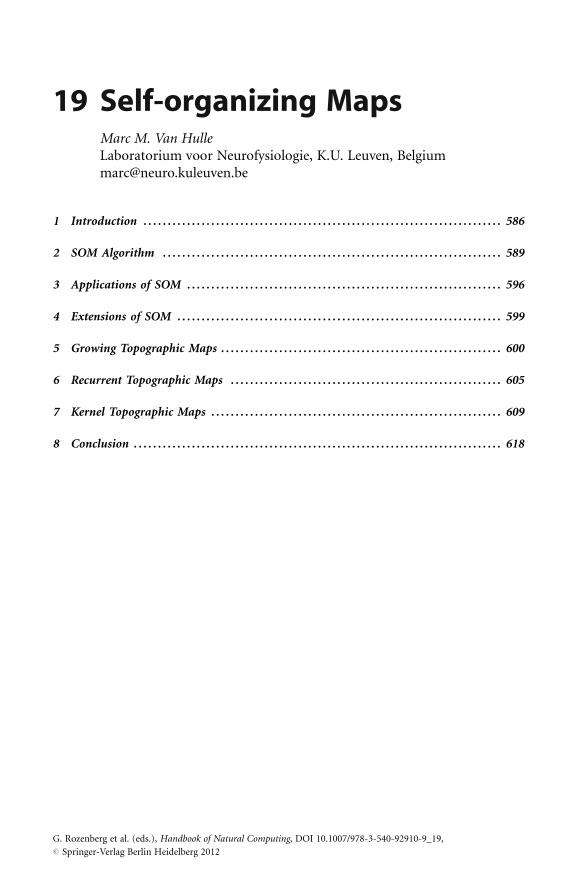
The study of topographic map formation, from a theoretical perspective, started with

basically two types of self-organizing processes, gradient-based learning and competitive

learning, and two types of network architectures (> Fig. 1) (for a review, see Van Hulle

[2000]). In the first architecture, which is commonly referred to as the Willshaw–von der

. Fig. 1

(a) Willshaw–von der Malsburg model. Two isomorphic, rectangular lattices of neurons are

shown: one represents the input layer and the other the output layer. Neurons are represented

by circles: filled circles denote active neurons (‘‘winning’’ neurons); open circles denote inactive

neurons. As a result of the weighted connections from the input to the output layer, the output

neurons receive different inputs from the input layer. Two input neurons are labeled (i, j) as

well as their corresponding output layer neurons (i0, j0). Neurons i and i0 are the only active

neurons in their respective layers. (b) Kohonen model. The common input all neurons receive is

directly represented in the input space, v 2 V � d . The ‘‘winning’’ neuron is labeled as i�: itsweight (vector) is the one that best matches the current input (vector).

Self-organizing Maps 19 587

Malsburgmodel (Willshaw and von derMalsburg 1976), there are two sets of neurons, arranged

in two (one- or) two-dimensional layers or lattices (> Fig. 1a). (A lattice is an undirected

graph in which every non-border vertex has the same, fixed number of incident edges, and

which usually appears in the form of an array with a rectangular or simplex topology.)

Topographic map formation is concerned with learning a mapping for which neighboring

neurons in the input lattice are connected to neighboring neurons in the output lattice.

The second architecture is far more studied, and is also the topic of this chapter. Now we

have continuously valued inputs taken from the input spaced , or the data manifold V � d ,

which need not be rectangular or have the same dimensionality as the lattice to which it

projects (> Fig. 1b). To every neuron i of the lattice A corresponds a reference position in the

input space, called the weight vector wi ¼ ½wij � 2 d. All neurons receive the same input

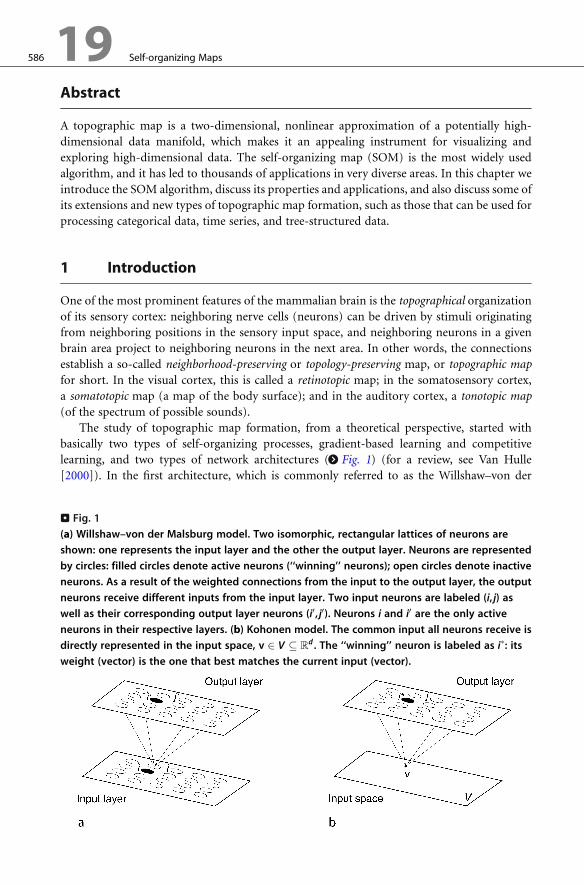
vector v ¼ ½v1; . . . ; vd � 2 V. Topographic map formation is concerned with learning a mapvA

of the data manifold V (gray shaded area in > Fig. 2), in such a way that neighboring lattice

neurons, i, j, with lattice positions ri,rj, code for neighboring positions, wi,wj, in the input

space (cf., the inverse mapping, C). The forward mapping, F, from the input space to the

lattice is not necessarily topology-preserving – neighboring weights do not necessarily corre-

spond to neighboring lattice neurons – even after learning the map, due to the possible

mismatch in dimensionalities of the input space and the lattice (see, e.g., > Fig. 3). In practice,

the map is represented in the input space in terms of neuron weights that are connected by

straight lines, if the corresponding neurons are the nearest neighbors in the lattice (e.g., see the

left panel of > Fig. 2 or > Fig. 3). When the map is topology preserving, it can be used for

visualizing the data distribution by projecting the original data points onto the map. The

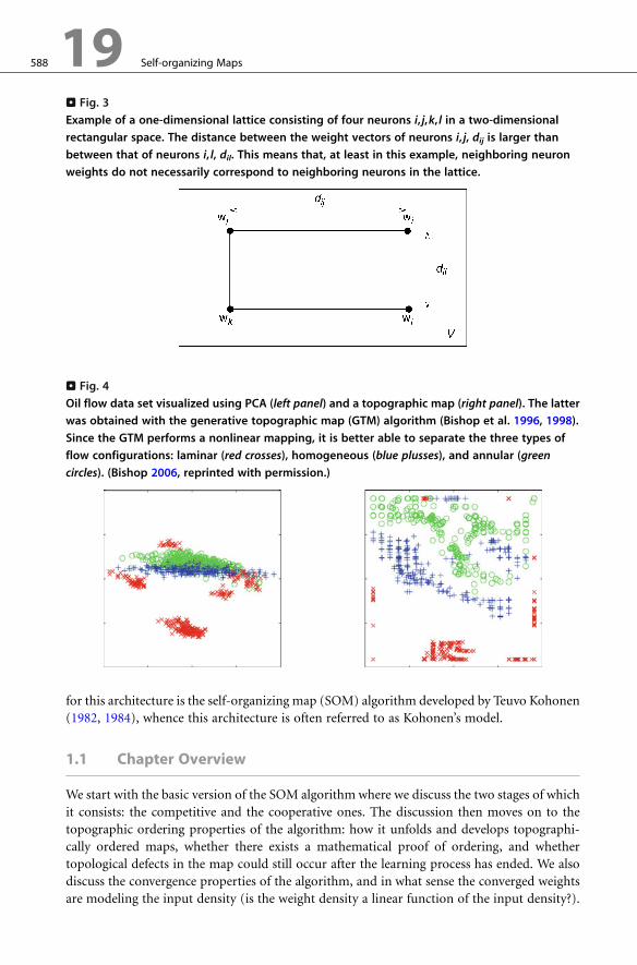
advantage of having a flexible map, compared to, for example, a plane specified by principal

components analysis (PCA), is demonstrated in > Fig. 4. We observe that the three classes are

better separated with a topographic map than with PCA. The most popular learning algorithm

. Fig. 2

Topographic mapping in the Kohonen architecture. In the left panel, the topology-preserving

mapvA of the data manifold V � d (gray-shaded area) is shown. The neuron weights,wi,wj, are

connected by a straight line since the corresponding neurons i, j in the lattice A (right panel), with

lattice coordinates ri,rj, are nearest neighbors. The forward mappingF is from the input space to

the lattice; the backward mapping C is from the lattice to the input space. The learning

algorithm tries to make neighboring lattice neurons, i, j, code for neighboring positions, wi,wj, in

the input space.

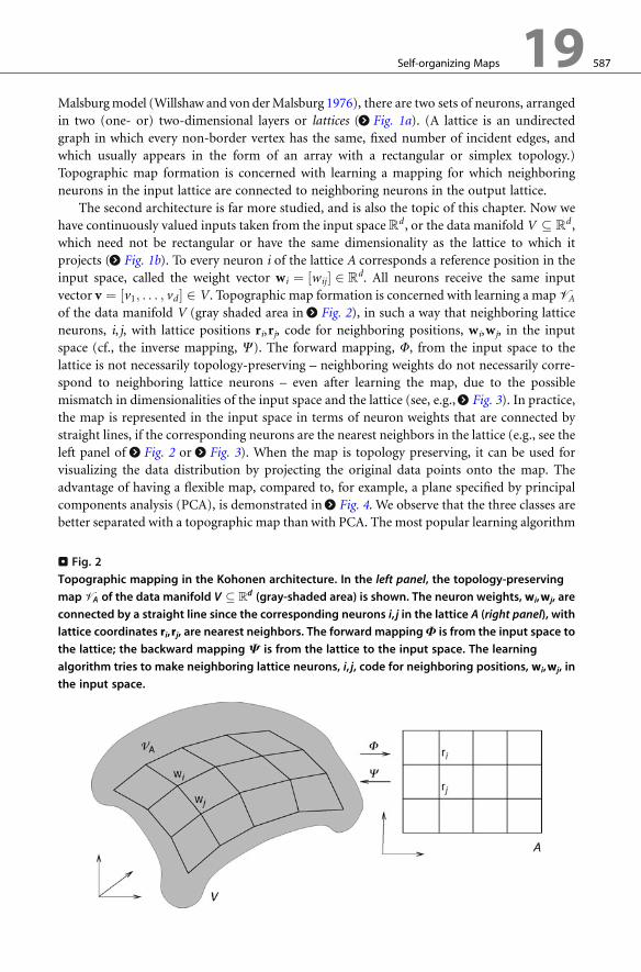
. Fig. 3

Example of a one-dimensional lattice consisting of four neurons i, j,k, l in a two-dimensional

rectangular space. The distance between the weight vectors of neurons i, j, dij is larger than

between that of neurons i, l, dil. This means that, at least in this example, neighboring neuron

weights do not necessarily correspond to neighboring neurons in the lattice.

. Fig. 4

Oil flow data set visualized using PCA (left panel) and a topographic map (right panel). The latter

was obtained with the generative topographic map (GTM) algorithm (Bishop et al. 1996, 1998).

Since the GTM performs a nonlinear mapping, it is better able to separate the three types of

flow configurations: laminar (red crosses), homogeneous (blue plusses), and annular (green

circles). (Bishop 2006, reprinted with permission.)


for this architecture is the self-organizing map (SOM) algorithm developed by Teuvo Kohonen

(1982, 1984), whence this architecture is often referred to as Kohonen’s model.

1.1 Chapter Overview

We start with the basic version of the SOM algorithm where we discuss the two stages of which

it consists: the competitive and the cooperative ones. The discussion then moves on to the

topographic ordering properties of the algorithm: how it unfolds and develops topographi-

cally ordered maps, whether there exists a mathematical proof of ordering, and whether

topological defects in the map could still occur after the learning process has ended. We also

discuss the convergence properties of the algorithm, and in what sense the converged weights

are modeling the input density (is the weight density a linear function of the input density?).


We then discuss applications of the SOM algorithm, thousands of which have been

reported in the open literature. Rather than attempting an extensive overview, the applications

are grouped into three areas: vector quantization, regression, and clustering. The latter is the

most important one since it is a direct consequence of the data visualization and exploration

capabilities of the topographic map. A number of important applications are highlighted,

such as WEBSOM (self-organizing maps for internet exploration) (Kaski et al. 1998) for

organizing large document collections; PicSOM (Laaksonen et al. 2002) for content-based

image retrieval; and the emergent self-organizing maps (ESOM) (Ultsch and Morchen 2005),

for which the MusicMiner (Risi et al. 2007) is considered, for organizing large collections of

music, and an application for classifying police reports of criminal incidents.

Later, an overview of a number of extensions of the SOM algorithm is given. The

motivation behind these is to improve the original algorithm, or to extend its range of

applications, or to develop new ways to perform topographic map formation.

Three important extensions of the SOM algorithm are then given in detail. First, we

discuss the growing topographic map algorithms. These algorithms consider maps with a

dynamically defined topology so as to better capture the fine structure of the input distribu-

tion. Second, since many input sources have a temporal characteristic, which is not captured

by the original SOM algorithm, several algorithms have been developed based on a recurrent

processing of time signals (recurrent topographic maps). It is a heavily researched area since

some of these algorithms are capable of processing tree-structured data. Third, another topic

of current research is the kernel topographic map, which is in line with the ‘‘kernelization’’

trend of mapping data into a feature space. Rather than Voronoi regions, the neurons are

equipped with overlapping activation regions, in the form of kernel functions, such as

Gaussians. Important future developments are expected for these topographic maps, such as

the visualization and clustering of structure-based molecule descriptions, and other biochem-

ical applications.

Finally, a conclusion to the chapter is formulated.

2 SOM Algorithm

The SOM algorithm distinguishes two stages: the competitive stage and the cooperative stage. In

the first stage, the best matching neuron is selected, that is, the ‘‘winner,’’ and in the second

stage, the weights of the winner are adapted as well as those of its immediate lattice neighbors.

Only the minimum Euclidean distance version of the SOM algorithm is considered (also the

dot product version exists, see Kohonen 1995).

2.1 Competitive Stage

For each input v 2V, the neuron with the smallest Euclidean distance (‘‘winner-takes-all,’’

WTA) is selected, which we call the ‘‘winner’’:

i� ¼ argmini

kwi � vk ð1Þ

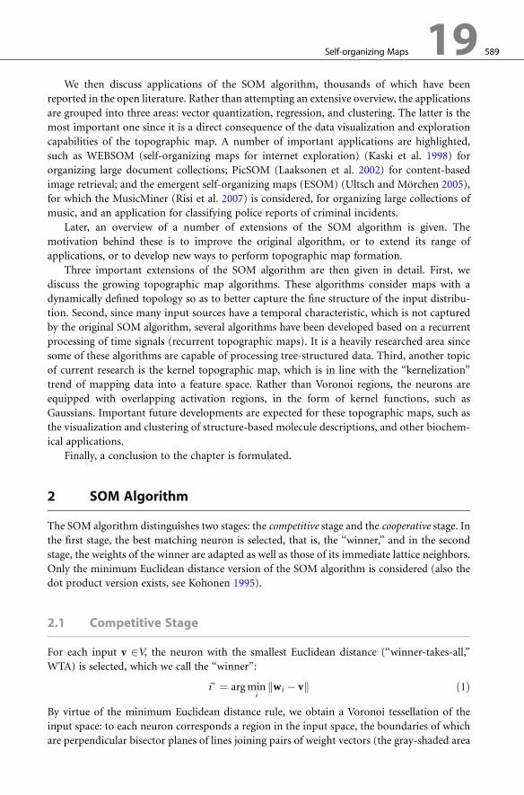
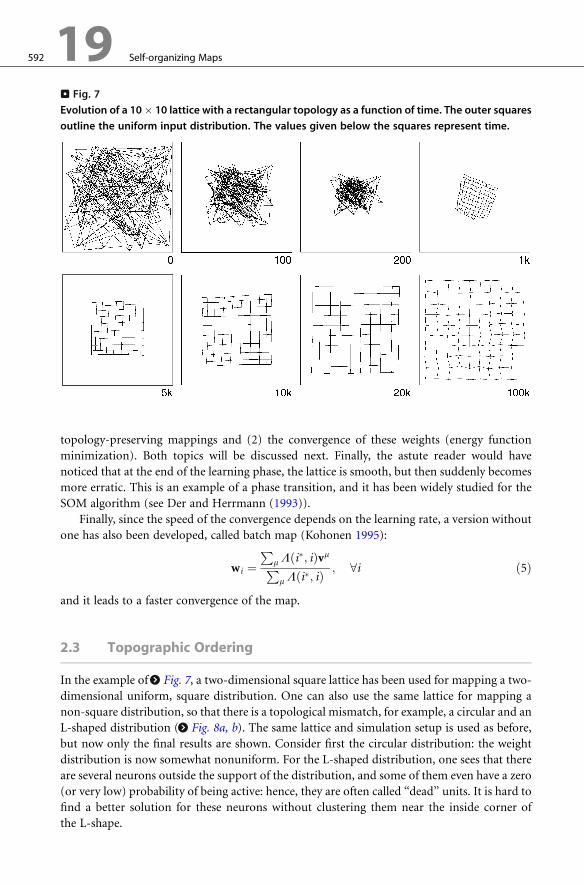
By virtue of the minimum Euclidean distance rule, we obtain a Voronoi tessellation of the

input space: to each neuron corresponds a region in the input space, the boundaries of which

are perpendicular bisector planes of lines joining pairs of weight vectors (the gray-shaded area


in > Fig. 5 is the Voronoi region of neuron j). Remember that the neuron weights are

connected by straight lines (links or edges): they indicate which neurons are nearest neighbors

in the lattice. These links are important for verifying whether the map is topology preserving.

2.2 Cooperative Stage

It is now crucial to the formation of topographically ordered maps that the neuron weights are

not modified independently of each other, but as topologically related subsets on which

similar kinds of weight updates are performed. During learning, not only the weight vector

of the winning neuron is updated, but also those of its lattice neighbors, which end up

responding to similar inputs. This is achieved with the neighborhood function, which is

centered at the winning neuron, and decreases with the lattice distance to the winning neuron.

(Besides the neighborhood function, also the neighborhood set exists, consisting of all

neurons to be updated in a given radius from the winning neuron [see Kohonen, (1995)].

The weight update rule in incremental mode is given by (with incremental mode we mean

that the weights are updated each time an input vector is presented, contrasted with batch

mode where the weights are only updated after the presentation of the full training set

[‘‘batch’’]):

Dwi ¼ � Lði; i�; sLðtÞÞ ðv � wiÞ; 8i 2 A ð2Þwith L the neighborhood function, that is, a scalar-valued function of the lattice coordinates

of neurons i and i�, ri and ri�, mostly a Gaussian:

Lði; i�Þ ¼ exp �kri � ri�k22s2

L

!ð3Þ

with range sL (i.e., the standard deviation). (we further drop the parameter sL(t) from the

neighborhood function to simplify the notation.) The positions ri are usually taken to be

. Fig. 5

Definition of quantization region in the self-organizing map (SOM). Portion of a lattice (thick

lines) plotted in terms of the weight vectors of neurons a; . . . ; k, in the two-dimensional

input space, that is, wa; . . . ;wk .


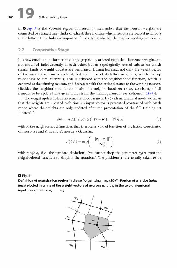
the nodes of a discrete lattice with a regular topology, usually a two-dimensional square or

rectangular lattice. An example of the effect of the neighborhood function in the weight

updates is shown in > Fig. 6 for a 4� 4 lattice. The parameter sL, and usually also the learning

rate �, are gradually decreased over time. When the neighborhood range vanishes, the previous

learning rule reverts to standard unsupervised competitive learning (UCL) (note that the latter

is unable to form topology-preserving maps, pointing to the importance of the neighborhood

function).

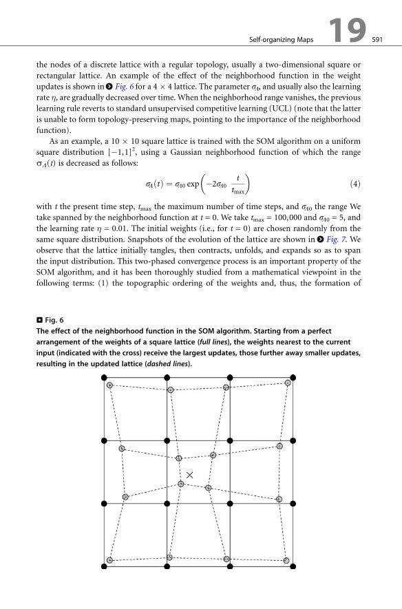
As an example, a 10 � 10 square lattice is trained with the SOM algorithm on a uniform

square distribution [�1,1]2, using a Gaussian neighborhood function of which the range

sL(t) is decreased as follows:

sLðtÞ ¼ sL0 exp �2sL0t

tmax

� �ð4Þ

with t the present time step, tmax the maximum number of time steps, and sL0 the range We

take spanned by the neighborhood function at t = 0. We take tmax = 100,000 and sL0 = 5, and

the learning rate � = 0.01. The initial weights (i.e., for t = 0) are chosen randomly from the

same square distribution. Snapshots of the evolution of the lattice are shown in > Fig. 7. We

observe that the lattice initially tangles, then contracts, unfolds, and expands so as to span

the input distribution. This two-phased convergence process is an important property of the

SOM algorithm, and it has been thoroughly studied from a mathematical viewpoint in the

following terms: (1) the topographic ordering of the weights and, thus, the formation of

. Fig. 6

The effect of the neighborhood function in the SOM algorithm. Starting from a perfect

arrangement of the weights of a square lattice (full lines), the weights nearest to the current

input (indicated with the cross) receive the largest updates, those further away smaller updates,

resulting in the updated lattice (dashed lines).

. Fig. 7

Evolution of a 10� 10 lattice with a rectangular topology as a function of time. The outer squares

outline the uniform input distribution. The values given below the squares represent time.


topology-preserving mappings and (2) the convergence of these weights (energy function

minimization). Both topics will be discussed next. Finally, the astute reader would have

noticed that at the end of the learning phase, the lattice is smooth, but then suddenly becomes

more erratic. This is an example of a phase transition, and it has been widely studied for the

SOM algorithm (see Der and Herrmann (1993)).

Finally, since the speed of the convergence depends on the learning rate, a version without

one has also been developed, called batch map (Kohonen 1995):

wi ¼P

m Lði�; iÞvmPm Lði�; iÞ

; 8i ð5Þ

and it leads to a faster convergence of the map.

2.3 Topographic Ordering

In the example of > Fig. 7, a two-dimensional square lattice has been used for mapping a two-

dimensional uniform, square distribution. One can also use the same lattice for mapping a

non-square distribution, so that there is a topological mismatch, for example, a circular and an

L-shaped distribution (> Fig. 8a, b). The same lattice and simulation setup is used as before,

but now only the final results are shown. Consider first the circular distribution: the weight

distribution is now somewhat nonuniform. For the L-shaped distribution, one sees that there

are several neurons outside the support of the distribution, and some of them even have a zero

(or very low) probability of being active: hence, they are often called ‘‘dead’’ units. It is hard to

find a better solution for these neurons without clustering them near the inside corner of

the L-shape.

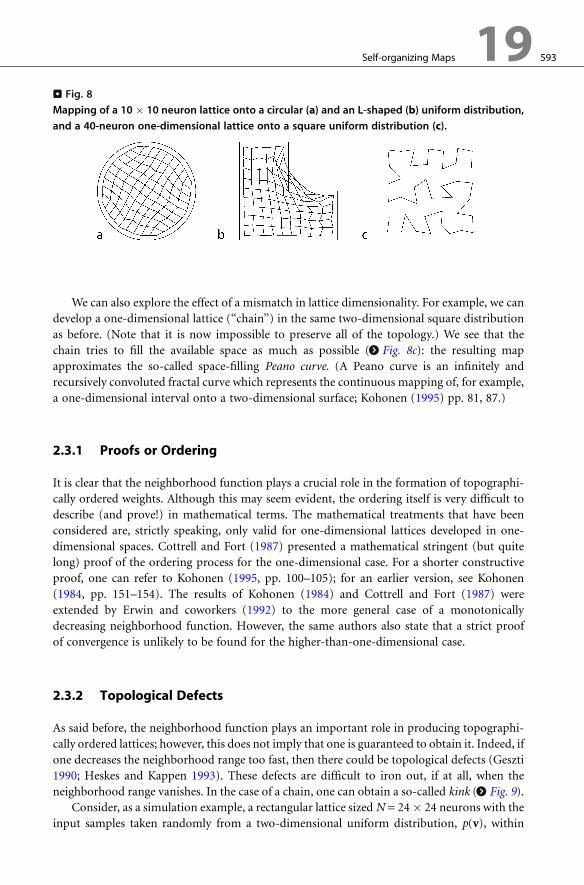
. Fig. 8

Mapping of a 10 � 10 neuron lattice onto a circular (a) and an L-shaped (b) uniform distribution,

and a 40-neuron one-dimensional lattice onto a square uniform distribution (c).


We can also explore the effect of a mismatch in lattice dimensionality. For example, we can

develop a one-dimensional lattice (‘‘chain’’) in the same two-dimensional square distribution

as before. (Note that it is now impossible to preserve all of the topology.) We see that the

chain tries to fill the available space as much as possible (> Fig. 8c): the resulting map

approximates the so-called space-filling Peano curve. (A Peano curve is an infinitely and

recursively convoluted fractal curve which represents the continuous mapping of, for example,

a one-dimensional interval onto a two-dimensional surface; Kohonen (1995) pp. 81, 87.)

2.3.1 Proofs or Ordering

It is clear that the neighborhood function plays a crucial role in the formation of topographi-

cally ordered weights. Although this may seem evident, the ordering itself is very difficult to

describe (and prove!) in mathematical terms. The mathematical treatments that have been

considered are, strictly speaking, only valid for one-dimensional lattices developed in one-

dimensional spaces. Cottrell and Fort (1987) presented a mathematical stringent (but quite

long) proof of the ordering process for the one-dimensional case. For a shorter constructive

proof, one can refer to Kohonen (1995, pp. 100–105); for an earlier version, see Kohonen

(1984, pp. 151–154). The results of Kohonen (1984) and Cottrell and Fort (1987) were

extended by Erwin and coworkers (1992) to the more general case of a monotonically

decreasing neighborhood function. However, the same authors also state that a strict proof

of convergence is unlikely to be found for the higher-than-one-dimensional case.

2.3.2 Topological Defects

As said before, the neighborhood function plays an important role in producing topographi-

cally ordered lattices; however, this does not imply that one is guaranteed to obtain it. Indeed, if

one decreases the neighborhood range too fast, then there could be topological defects (Geszti

1990; Heskes and Kappen 1993). These defects are difficult to iron out, if at all, when the

neighborhood range vanishes. In the case of a chain, one can obtain a so-called kink (> Fig. 9).

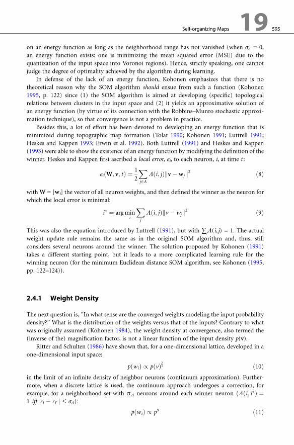
Consider, as a simulation example, a rectangular lattice sizedN = 24� 24 neurons with the

input samples taken randomly from a two-dimensional uniform distribution, p(v), within

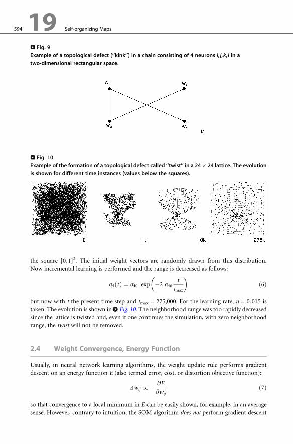
. Fig. 9

Example of a topological defect (‘‘kink’’) in a chain consisting of 4 neurons i, j,k, l in a

two-dimensional rectangular space.

. Fig. 10

Example of the formation of a topological defect called ‘‘twist’’ in a 24� 24 lattice. The evolution

is shown for different time instances (values below the squares).


the square [0,1]2. The initial weight vectors are randomly drawn from this distribution.

Now incremental learning is performed and the range is decreased as follows:

sLðtÞ ¼ sL0 exp �2 sL0t

tmax

� �ð6Þ

but now with t the present time step and tmax = 275,000. For the learning rate, � = 0.015 is

taken. The evolution is shown in > Fig. 10. The neighborhood range was too rapidly decreased

since the lattice is twisted and, even if one continues the simulation, with zero neighborhood

range, the twist will not be removed.

2.4 Weight Convergence, Energy Function

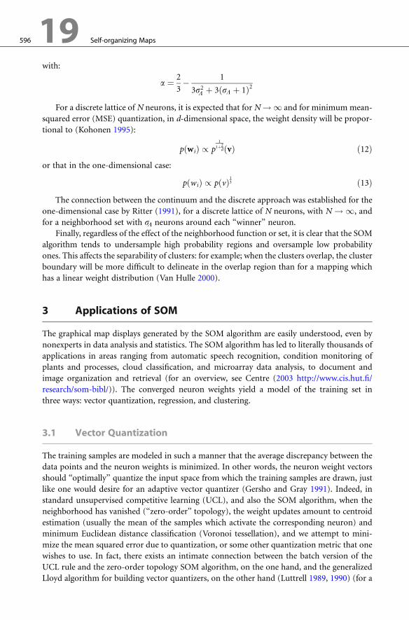
Usually, in neural network learning algorithms, the weight update rule performs gradient

descent on an energy function E (also termed error, cost, or distortion objective function):

Dwij / � @E

@wij

ð7Þ

so that convergence to a local minimum in E can be easily shown, for example, in an average

sense. However, contrary to intuition, the SOM algorithm does not perform gradient descent


on an energy function as long as the neighborhood range has not vanished (when sL = 0,

an energy function exists: one is minimizing the mean squared error (MSE) due to the

quantization of the input space into Voronoi regions). Hence, strictly speaking, one cannot

judge the degree of optimality achieved by the algorithm during learning.

In defense of the lack of an energy function, Kohonen emphasizes that there is no

theoretical reason why the SOM algorithm should ensue from such a function (Kohonen

1995, p. 122) since (1) the SOM algorithm is aimed at developing (specific) topological

relations between clusters in the input space and (2) it yields an approximative solution of

an energy function (by virtue of its connection with the Robbins–Munro stochastic approxi-

mation technique), so that convergence is not a problem in practice.

Besides this, a lot of effort has been devoted to developing an energy function that is

minimized during topographic map formation (Tolat 1990; Kohonen 1991; Luttrell 1991;

Heskes and Kappen 1993; Erwin et al. 1992). Both Luttrell (1991) and Heskes and Kappen

(1993) were able to show the existence of an energy function by modifying the definition of the

winner. Heskes and Kappen first ascribed a local error, ei, to each neuron, i, at time t :

eiðW; v; tÞ ¼ 1

2

Xj2A

Lði; jÞkv � wjk2 ð8Þ

withW = [wi] the vector of all neuron weights, and then defined the winner as the neuron for

which the local error is minimal:

i� ¼ argmini

Xj

Lði; jÞkv � wjk2 ð9Þ

This was also the equation introduced by Luttrell (1991), but with ∑jL(i, j) = 1. The actual

weight update rule remains the same as in the original SOM algorithm and, thus, still

considers several neurons around the winner. The solution proposed by Kohonen (1991)

takes a different starting point, but it leads to a more complicated learning rule for the

winning neuron (for the minimum Euclidean distance SOM algorithm, see Kohonen (1995,

pp. 122–124)).

2.4.1 Weight Density

The next question is, ‘‘In what sense are the converged weights modeling the input probability

density?’’ What is the distribution of the weights versus that of the inputs? Contrary to what

was originally assumed (Kohonen 1984), the weight density at convergence, also termed the

(inverse of the) magnification factor, is not a linear function of the input density p(v).

Ritter and Schulten (1986) have shown that, for a one-dimensional lattice, developed in a

one-dimensional input space:

pðwiÞ / pðvÞ23 ð10Þin the limit of an infinite density of neighbor neurons (continuum approximation). Further-

more, when a discrete lattice is used, the continuum approach undergoes a correction, for

example, for a neighborhood set with sL neurons around each winner neuron ðLði; i�Þ ¼1 iff jri � ri� j � sL):

pðwiÞ / pa ð11Þ


with:

a ¼ 2

3� 1

3s2L þ 3ðsL þ 1Þ2

For a discrete lattice of N neurons, it is expected that for N!1 and for minimum mean-

squared error (MSE) quantization, in d-dimensional space, the weight density will be propor-

tional to (Kohonen 1995):

pðwiÞ / p1

1þ2dðvÞ ð12Þ

or that in the one-dimensional case:

pðwiÞ / pðvÞ13 ð13ÞThe connection between the continuum and the discrete approach was established for the

one-dimensional case by Ritter (1991), for a discrete lattice of N neurons, with N ! 1, and

for a neighborhood set with sL neurons around each ‘‘winner’’ neuron.

Finally, regardless of the effect of the neighborhood function or set, it is clear that the SOM

algorithm tends to undersample high probability regions and oversample low probability

ones. This affects the separability of clusters: for example; when the clusters overlap, the cluster

boundary will be more difficult to delineate in the overlap region than for a mapping which

has a linear weight distribution (Van Hulle 2000).

3 Applications of SOM

The graphical map displays generated by the SOM algorithm are easily understood, even by

nonexperts in data analysis and statistics. The SOM algorithm has led to literally thousands of

applications in areas ranging from automatic speech recognition, condition monitoring of

plants and processes, cloud classification, and microarray data analysis, to document and

image organization and retrieval (for an overview, see Centre (2003 http://www.cis.hut.fi/

research/som-bibl/)). The converged neuron weights yield a model of the training set in

three ways: vector quantization, regression, and clustering.

3.1 Vector Quantization

The training samples are modeled in such a manner that the average discrepancy between the

data points and the neuron weights is minimized. In other words, the neuron weight vectors

should ‘‘optimally’’ quantize the input space from which the training samples are drawn, just

like one would desire for an adaptive vector quantizer (Gersho and Gray 1991). Indeed, in

standard unsupervised competitive learning (UCL), and also the SOM algorithm, when the

neighborhood has vanished (‘‘zero-order’’ topology), the weight updates amount to centroid

estimation (usually the mean of the samples which activate the corresponding neuron) and

minimum Euclidean distance classification (Voronoi tessellation), and we attempt to mini-

mize the mean squared error due to quantization, or some other quantization metric that one

wishes to use. In fact, there exists an intimate connection between the batch version of the

UCL rule and the zero-order topology SOM algorithm, on the one hand, and the generalized

Lloyd algorithm for building vector quantizers, on the other hand (Luttrell 1989, 1990) (for a

http://www.cis.hut.fi/research/som-bibl/



review, see Van Hulle (2000)). Luttrell showed that the neighborhood function can be

considered as a probability density function of which the range is chosen to capture the

noise process responsible for the distortion of the quantizer’s output code (i.e., the index of the

winning neuron), for example, due to noise in the communication channel. Luttrell adopted

for the noise process a zero-mean Gaussian, so that there is theoretical justification for

choosing a Gaussian neighborhood function in the SOM algorithm.

3.2 Regression

One can also interpret the map as a case of non-parametric regression: no prior knowledge is

assumed about the nature or shape of the function to be regressed. Non-parametric regression

is perhaps the first successful statistical application of the SOM algorithm (Ritter et al. 1992;

Mulier and Cherkassky 1995; Kohonen 1995): the converged topographic map is intended to

capture the principal dimensions (principal curves and principal manifolds) of the input

space. The individual neurons represent the ‘‘knots’’ that join piecewise smooth functions,

such as splines, which act as interpolating functions for generating values at intermediate

positions. Furthermore, the lattice coordinate system can be regarded as an (approximate)

global coordinate system of the data manifold (> Fig. 2).

3.3 Clustering

The most widely used application of the topographic map is clustering, that is, the partitioning

of the data set into subsets of ‘‘similar’’ data, without using prior knowledge about these

subsets. One of the first demonstrations of clustering was by Ritter and Kohonen (1989). They

had a list of 16 animals (birds, predators, and preys) and 13 binary attributes for each one of

them (e.g., large size or not, hair or not, two legged or not, can fly or not, etc.). After training a

10� 10 lattice of neurons with these vectors (supplemented with the 1-out-of-16 animal code

vector, thus, in total, a 29-dimensional binary vector), and labeling the winning neuron for

each animal code vector, a natural clustering of birds, predators, and prey appeared in the

map. The authors called this the ‘‘semantic map.’’

In the previous application, the clusters and their boundaries were defined by the user. In

order to visualize clusters more directly, one needs an additional technique. One can compute

the mean Euclidean distance between a neuron’s weight vector and the weight vectors of its

nearest neighbors in the lattice. The maximum and minimum of the distances found for all

neurons in the lattice is then used for scaling these distances between 0 and 1; the lattice then

becomes a gray scale image with white pixels corresponding to, for example, 0 and black pixels

to 1. This is called the U-matrix (Ultsch and Siemon 1990), for which several extensions have

been developed to remedy the oversampling of low probability regions (possibly transition

regions between clusters) (Ultsch and Morchen 2005).

An important example is WEBSOM (Kaski et al. 1998). Here, the SOM is used for

organizing document collections (‘‘document map’’). Each document is represented as a

vector of keyword occurrences. Similar documents then become grouped into the same cluster.

After training, the user can zoom into the map to inspect the clusters. The map is manually or

automatically labeled with keywords (e.g., from a man-made list) in such a way that, at each

zoom level, the same density of keywords is shown (so as not to clutter the map with text).


WEBSOM has also been applied to visualizing clusters in patents based on keyword occur-

rences in patent abstracts (Kohonen et al. 1999).

An example of a content-based image retrieval system is the PicSOM (Laaksonen et al.

2002). Here, low-level features (color, shape, texture, etc.) of each image are considered.

A separate two-dimensional SOM is trained for each low-level feature (in fact, a hierarchical

SOM). In order to be able to retrieve one particular image from the database, one is faced with

a semantic gap: how well do the low-level features correlate with the image contents? To bridge

this gap, relevance feedback is used: the user is shown a number of images and he/she has to

decide which ones are relevant and which ones are not (close or not to the image the user is

interested in). Based on the trained PicSOM, the next series of images shown are then

supposed to be more relevant, and so on.

For high-dimensional data visualization, a special class of topographic maps called

emergent self-organizing maps (ESOM) (Ultsch and Morchen 2005) can be considered.

According to Ultsch, emergence is the ability of a system to produce a phenomenon on a

new, higher level. In order to achieve emergence, the existence and cooperation of a large

number of elementary processes is necessary. An emergent SOM differs from the traditional

SOM in that a very large number of neurons (at least a few thousand) are used (even larger

than the number of data points). The ESOM software is publicly available from http://

databionic-esom.sourceforge.net/.

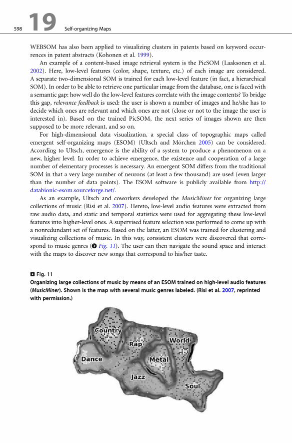
As an example, Ultsch and coworkers developed the MusicMiner for organizing large

collections of music (Risi et al. 2007). Hereto, low-level audio features were extracted from

raw audio data, and static and temporal statistics were used for aggregating these low-level

features into higher-level ones. A supervised feature selection was performed to come up with

a nonredundant set of features. Based on the latter, an ESOM was trained for clustering and

visualizing collections of music. In this way, consistent clusters were discovered that corre-

spond to music genres (> Fig. 11). The user can then navigate the sound space and interact

with the maps to discover new songs that correspond to his/her taste.

. Fig. 11

Organizing large collections of music by means of an ESOM trained on high-level audio features

(MusicMiner). Shown is the map with several music genres labeled. (Risi et al. 2007, reprinted

with permission.)

http://databionic-esom.sourceforge.net/

http://databionic-esom.sourceforge.net/


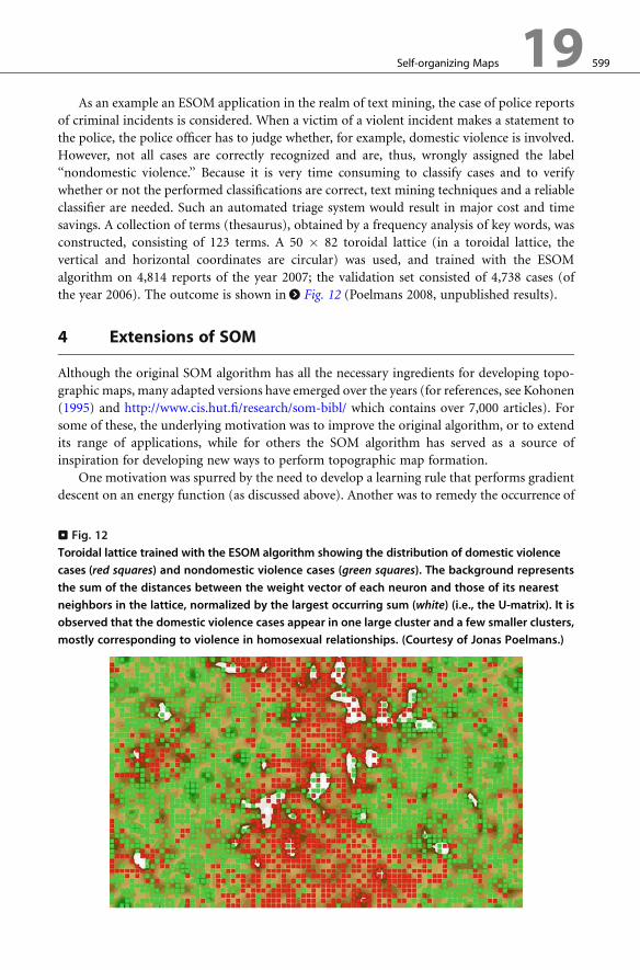
As an example an ESOM application in the realm of text mining, the case of police reports

of criminal incidents is considered. When a victim of a violent incident makes a statement to

the police, the police officer has to judge whether, for example, domestic violence is involved.

However, not all cases are correctly recognized and are, thus, wrongly assigned the label

‘‘nondomestic violence.’’ Because it is very time consuming to classify cases and to verify

whether or not the performed classifications are correct, text mining techniques and a reliable

classifier are needed. Such an automated triage system would result in major cost and time

savings. A collection of terms (thesaurus), obtained by a frequency analysis of key words, was

constructed, consisting of 123 terms. A 50 � 82 toroidal lattice (in a toroidal lattice, the

vertical and horizontal coordinates are circular) was used, and trained with the ESOM

algorithm on 4,814 reports of the year 2007; the validation set consisted of 4,738 cases (of

the year 2006). The outcome is shown in > Fig. 12 (Poelmans 2008, unpublished results).

4 Extensions of SOM

Although the original SOM algorithm has all the necessary ingredients for developing topo-

graphic maps, many adapted versions have emerged over the years (for references, see Kohonen

(1995) and http://www.cis.hut.fi/research/som-bibl/ which contains over 7,000 articles). For

some of these, the underlying motivation was to improve the original algorithm, or to extend

its range of applications, while for others the SOM algorithm has served as a source of

inspiration for developing new ways to perform topographic map formation.

One motivation was spurred by the need to develop a learning rule that performs gradient

descent on an energy function (as discussed above). Another was to remedy the occurrence of

. Fig. 12

Toroidal lattice trained with the ESOM algorithm showing the distribution of domestic violence

cases (red squares) and nondomestic violence cases (green squares). The background represents

the sum of the distances between the weight vector of each neuron and those of its nearest

neighbors in the lattice, normalized by the largest occurring sum (white) (i.e., the U-matrix). It is

observed that the domestic violence cases appear in one large cluster and a few smaller clusters,

mostly corresponding to violence in homosexual relationships. (Courtesy of Jonas Poelmans.)



dead units, since they do not contribute to the representation of the input space (or the data

manifold). Several researchers were inspired by Grossberg’s idea (1976) of adding a ‘‘conscience’’

to frequently winning neurons to feel ‘‘guilty’’ and to reduce their winning rates. The same

heuristic idea has also been adopted in combination with topographic map formation

(DeSieno 1988; Van den Bout and Miller 1989; Ahalt et al. 1990). Others exploit measures

based on the local distortion error to equilibrate the neurons’ ‘‘conscience’’ (Kim and Ra 1995;

Chinrungrueng and Sequin 1995; Ueda and Nakano 1993). A combination of the two

conscience approaches is the learning scheme introduced by Bauer and coworkers (1996).

A different strategy is to apply a competitive learning rule that minimizes themean absolute

error (MAE) between the input samples v and the N weight vectors (also called theMinkowski

metric of power one) (Kohonen 1995, pp. 120, 121) (see also Lin et al. (1997)). Instead of

minimizing a (modified) distortion criterion, a more natural approach is to optimize an

information-theoretic criterion directly. Linsker was among the first to explore this idea in the

context of topographic map formation. He proposed a principle of maximum information

preservation (Linsker 1988) – infomax for short – according to which a processing stage has the

property that the output signals will optimally discriminate, in an information-theoretic

sense, among possible sets of input signals applied to that stage. In his 1989 article, he devised

a learning rule for topographic map formation in a probabilistic WTA network by maximizing

the average mutual information between the output and the signal part of the input, which

was corrupted by noise (Linsker 1989). Another algorithm is the vectorial boundary adapta-

tion rule (VBAR) which considers the region spanned by a quadrilateral (four neurons

forming a square region in the lattice) as the quantization region (Van Hulle 1997a, b), and

which is able to achieve an equiprobabilistic map, that is, a map for which every neuron has

the same chance to be active (and, therefore, maximizes the information-theoretic entropy).

Another evolution is the growing topographic map algorithms. In contrast to the original

SOM algorithm, its growing map variants have a dynamically defined topology, and they are

believed to better capture the fine structure of the input distribution. They will be discussed in

the next section.

Many input sources have a temporal characteristic, which is not captured by the original

SOM algorithm. Several algorithms have been developed based on a recurrent processing of

time signals and a recurrent winning neuron computation. Also tree structured data can be

represented with such topographic maps. Recurrent topographic maps will be discussed in this

chapter.

Another important evolution is the kernel-based topographic maps: rather than Voronoi

regions, the neurons are equipped with overlapping activation regions, usually in the form of

kernel functions, such as Gaussians (> Fig. 19). Also for this case, several algorithms have been

developed, and a number of them will be discussed in this chapter.

5 Growing Topographic Maps

In order to overcome the topology mismatches that occur with the original SOM algorithm, as

well as to achieve an optimal use of the neurons (cf., dead units), the geometry of the lattice has

tomatch that of the datamanifold it is intended to represent. For that purpose, several so-called

growing (incremental or structure-adaptive) self-organizing map algorithms have been devel-

oped. What they share is that the lattices are gradually built up and, hence, do not have a

predefined structure (i.e., number of neurons and possibly also lattice dimensionality)


(> Fig. 14). The lattice is generated by a successive insertion (andpossibly an occasional deletion)

of neurons and connections between them. Some of these algorithms can even guarantee that the

lattice is free of topological defects (e.g., since the lattice is a subgraph of a Delaunay triangular-

ization, see further). The major algorithms for growing self-organizing maps will be briefly

reviewed. The algorithms are structurally not very different; the main difference is with the

constraints imposed on the lattice topology (fixed or variable lattice dimensionality). The

properties common to these algorithms are first listed, using the format suggested by Fritzke

(1996).

� The network is an undirected graph (lattice) consisting of a number of nodes (neurons)

and links or edges connecting them.

� Each neuron, i, has a weight vector wi in the input space V.

� The weight vectors are updated by moving the winning neuron i�, and its topological

neighbors, toward the input v2V:Dwi� ¼ �i� ðv � wi� Þ ð14Þ

Dwi ¼ �iðv � wiÞ; 8i 2 ni� ð15Þ

withni� the set of direct topological neighbors of neuron i� (neighborhood set), and with

�i� and �i the learning rates, �i��i .

� At each time step, the local error at the winning neuron, i�, is accumulated:

DEi� ¼ ðerror measureÞ ð16ÞThe error term is coming from a particular area around wi� , and is likely to be reduced by

inserting new neurons in that area. A central property of these algorithms is the possibility

to choose an arbitrary error measure as the basis for insertion. This extends their applica-

tions from unsupervised learning ones, such as data visualization, combinatorial optimi-

zation, and clustering analysis, to supervised learning ones, such as classification and

regression. For example, for vector quantization, DEi� ¼ kv � wi�k2. For classification,

the obvious choice is the classification error. All models reviewed here can, in principle, be

used for supervised learning applications by associating output values to the neurons, for

example, through kernels such as radial basis functions. This makes most sense for the

algorithms that adapt their dimensionality to the data.

� The accumulated error of each neuron is used to determine (after a fixed number of time

steps) where to insert new neurons in the lattice. After an insertion, the error information

is locally redistributed, which increases the probability that the next insertion will be

somewhere else. The local error acts as a kind of memory where much error has occurred;

the exponential decay of the error stresses more the recently accumulated error.

� All parameters of the algorithm stay constant over time.

5.1 Competitive Hebbian Learning and Neural Gas

Historically, the first algorithm to develop topologies was introduced by Martinetz and

Schulten, and it is a combination of two methods: competitive Hebbian learning (CHL)

(Martinetz 1993) and the neural gas (NG) (Martinetz and Schulten 1991).


The principle behind CHL is simple: for each input, create a link between the winning

neuron and the second winning neuron (i.e., with the second smallest Euclidean distance to

the input), if that link does not already exist. Only weight vectors lying in the data manifold

develop links between them (thus, nonzero input density regions). The resulting graph is a

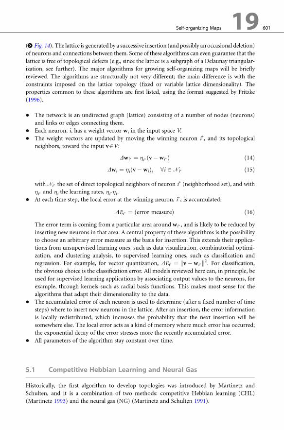
subgraph of the (induced) Delaunay triangularization (> Fig. 13), and it has been shown to

optimally preserve topology in a very general sense.

In order to position the weight vectors in the input space, Martinetz and Schulten (1991)

have proposed a particular kind of vector quantization method, called neural gas (NG). The

main principle of NG is for each input v update the k nearest-neighbor neuron weight vectors,

with k decreasing over time until only the winning neuron’s weight vector is updated. Hence,

one has a neighborhood function but now in input space. The learning rate also follows a

decay schedule. Note that the NG by itself does not delete or insert any neurons. The NG

requires finetuning of the rate at which the neighborhood shrinks to achieve a smooth

convergence and proper modeling of the data manifold.

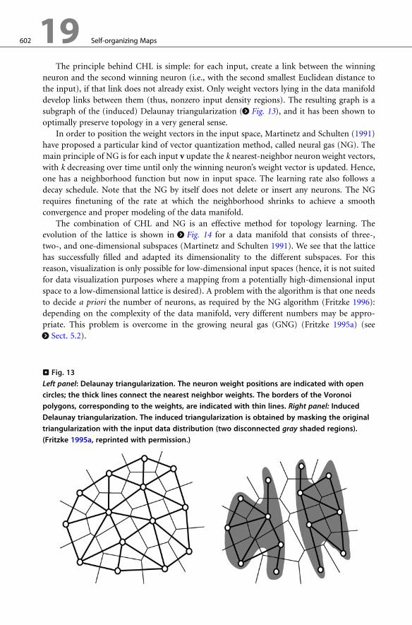
The combination of CHL and NG is an effective method for topology learning. The

evolution of the lattice is shown in > Fig. 14 for a data manifold that consists of three-,

two-, and one-dimensional subspaces (Martinetz and Schulten 1991). We see that the lattice

has successfully filled and adapted its dimensionality to the different subspaces. For this

reason, visualization is only possible for low-dimensional input spaces (hence, it is not suited

for data visualization purposes where a mapping from a potentially high-dimensional input

space to a low-dimensional lattice is desired). A problem with the algorithm is that one needs

to decide a priori the number of neurons, as required by the NG algorithm (Fritzke 1996):

depending on the complexity of the data manifold, very different numbers may be appro-

priate. This problem is overcome in the growing neural gas (GNG) (Fritzke 1995a) (see> Sect. 5.2).

. Fig. 13

Left panel: Delaunay triangularization. The neuron weight positions are indicated with open

circles; the thick lines connect the nearest neighbor weights. The borders of the Voronoi

polygons, corresponding to the weights, are indicated with thin lines. Right panel: Induced

Delaunay triangularization. The induced triangularization is obtained by masking the original

triangularization with the input data distribution (two disconnected gray shaded regions).

(Fritzke 1995a, reprinted with permission.)

. Fig. 14

Neural gas algorithm, combined with competitive Hebbian learning, applied to a data manifold

consisting of a right parallelepiped, a rectangle, and a circle connecting a line. The dots indicate

the positions of the neuron weights. Lines connecting neuron weights indicate lattice edges.

Shown are the initial result (top left), and further the lattice after 5,000, 10,000, 15,000, 25,000,

and 40,000 time steps (top-down the first column, then top-down the second column). (Martinetz

and Schulten 1991, reprinted with permission.)


5.2 Growing Neural Gas

Contrary to CHL/NG, the growing neural gas (GNG) poses no explicit constraints on the

lattice. The lattice is generated, and constantly updated, by the competitive Hebbian learning

technique (CHL, see above; Martinetz 1993). The algorithm starts with two randomly placed

and connected neurons (> Fig. 15, left panel). Unlike the CHL/NG algorithm, after a fixed

number, l, of time steps, the neuron, i, with the largest accumulated error is determined and a

new neuron inserted between i and one of its neighbors. Hence, the GNG algorithm exploits

the topology to position new neurons between existing ones, whereas in the CHL/NG the

topology is not influenced by the NG algorithm. Error variables are locally redistributed

and another l time step is performed. The lattice generated is a subgraph of a Delaunay

triangularization, and can have different dimensionalities in different regions of the data

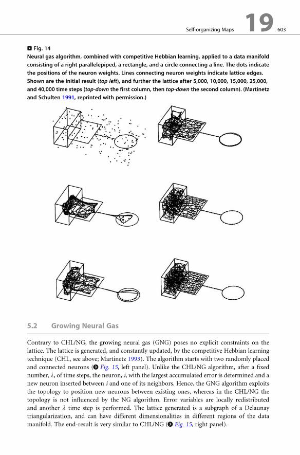
manifold. The end-result is very similar to CHL/NG (> Fig. 15, right panel).

. Fig. 15

Growing neural gas algorithm applied to the same data configuration as in > Fig. 14. Initial

lattice (left panel) and lattice after 20,000 time steps (right panel). Note that the last one is not

necessarily the final result because the algorithm could run indefinitely. (Fritzke 1995a, reprinted

with permission.)


5.3 Growing Cell Structures

In the growing cell structures (GCS) algorithm (Fritzke 1994), the model consists of hyperte-

trahedrons (or simplices) of a dimensionality chosen in advance (hence, the lattice dimension-

ality is fixed). Note that a dA-dimensional hypertetrahedron has dA+1 vertices, with dA the

lattice dimensionality, and dA�d, with d the input space dimensionality. Examples for d = 1, 2,

and 3 are a line, a triangle, and a tetrahedron, respectively.

The model is initialized with exactly one hypertetrahedron. Always after a prespecified

number of time steps, the neuron, i, with the maximum accumulated error is determined

and a new neuron is inserted by splitting the longest of the edges emanating from i.

Additional edges are inserted to rebuild the structure in such a way that it consists only of

dA-dimensional hypertetrahedrons: Let the edge which is split connect neurons i and j, then

the newly inserted neuron should be connected to i and j and with all common topological

neighbors of i and j.

Since the GCS algorithm assumes a fixed dimensionality for the lattice, it can be used for

generating a dimensionality reducing mapping from the input space to the lattice space, which

is useful for data visualization purposes.

5.4 Growing Grid

In the growing grid algorithm (GG) (Fritzke 1995b), the lattice is a rectangular grid of a certain

dimensionality dA. The starting configuration is a dA-dimensional hypercube, for example, a

2 � 2 lattice for dA = 2, a 2 � 2 � 2 lattice for dA = 3, and so on. To keep this structure

consistent, it is necessary to always insert complete (hyper-)rows and (hyper-)columns. Since

the lattice dimensionality is fixed, and possibly much smaller than the input space dimension-

ality, the GG is useful for data visualization.

Apart from these differences, the algorithm is very similar to the ones described above.

After l time steps, the neuron with the largest accumulated error is determined, and the

longest edge emanating from it is identified, and a new complete hyper-row or -column is

inserted such that the edge is split.


5.5 Other Algorithms

There exists a wealth of other algorithms, such as the dynamic cell structures (DCS) (Bruske

and Sommer 1995), which is similar to the GNG; the growing self-organizing map (GSOM,

also called hypercubical SOM) (Bauer and Villmann 1997), which has some similarities to GG

but it adapts the lattice dimensionality; incremental grid growing (IGG), which introduces

new neurons at the lattice border and adds/removes connections based on the similarities of

the connected neurons’ weight vectors (Blackmore and Miikkulainen 1993); and one that is

also called the growing self-organizing map (GSOM) (Alahakoon et al. 2000), which also adds

new neurons at the lattice border, similar to IGG, but does not delete neurons, and which

contains a spread factor to let the user control the spread of the lattice.

In order to study and exploit hierarchical relations in the data, hierarchical versions of some

of these algorithms have been developed. For example, the growing hierarchical self-organizing

map (GHSOM) (Rauber et al. 2002) develops lattices at each level of the hierarchy using the

GG algorithm (insertion of columns or rows). The orientation in space of each lattice is similar

to that of the parent lattice, which facilitates the interpretation of the hierarchy, and which is

achieved through a careful initialization of each lattice. Another example is adaptive hierar-

chical incremental grid growing (AHIGG) (Merkl et al. 2003) of which the hierarchy consists

of lattices trained with the IGG algorithm, and for which new units at a higher level are

introduced when the local (quantization) error of a neuron is too large.

6 Recurrent Topographic Maps

6.1 Time Series

Many data sources such as speech have a temporal characteristic (e.g., a correlation structure)

that cannot be sufficiently captured when ignoring the order in which the data points arrive, as

in the original SOM algorithm. Several self-organizing map algorithms have been developed

for dealing with sequential data, such as those using:

� fixed-length windows, for example, the time-delayed SOM (Kangas 1990), among others

(Martinetz et al. 1993; Simon et al. 2003; Vesanto 1997);

� specific sequence metrics (Kohonen 1997; Somervuo 2004);

� statistical modeling incorporating appropriate generative models for sequences (Bishop

et al. 1997; Tino et al. 2004);

� mapping of temporal dependencies to spatial correlation, for example, as in traveling

wave signals or potentially trained, temporally activated lateral interactions (Euliano and

Principe 1999; Schulz and Reggia 2004; Wiemer 2003);

� recurrent processing of time signals and recurrent winning neuron computation based on

the current input and the previous map activation, such as with the temporal Kohonen

map (TKM) (Chappell and Taylor 1993), the recurrent SOM (RSOM) (Koskela et al.

1998), the recursive SOM (RecSOM) (Voegtlin 2002), the SOM for structured data

(SOMSD) (Hagenbuchner et al. 2003), and the merge SOM (MSOM) (Strickert and

Hammer 2005).

Several of these algorithms proposed recently, which shows the increased interest in

representing time series with topographic maps. For some of these algorithms, also tree


structured data can be represented (see later). We focus on the recurrent processing of time

signals, and we briefly describe the models listed. A more detailed overview can be found

elsewhere (Barreto and Araujo 2001; Hammer et al. 2005). The recurrent algorithms essential-

ly differ in the context, that is, the way by which sequences are internally represented.

6.1.1 Overview of Algorithms

The TKM extends the SOM algorithm with recurrent self-connections of the neurons, such

that they act as leaky integrators (> Fig. 16a). Given a sequence ½v1; . . . ; vt �, vj 2 d ; 8j, theintegrated distance IDi of neuron i with weight vector wi 2 d is:

IDiðtÞ ¼ akvt � wik2 þ ð1� aÞIDiðt � 1Þ ð17Þwith a2(0,1) a constant determining the strength of the context information, and with

IDið0Þ ¼D 0. The winning neuron is selected as i�(t) = argminIIDi(t), after which the network

is updated as in the SOM algorithm. > Equation 17 has the form of a leaky integrator,

integrating previous distances of neuron i, given the sequence.

The RSOM uses, in essence, the same dynamics; however, it integrates over the directions

of the individual weight components:

IDijðtÞ ¼ aðvjt � wiÞ þ ð1� aÞIDijðt � 1Þ ð18Þso that the winner is then the neuron for which k½IDijðtÞ�k2 is the smallest. It is clear that this

algorithm stores more information than the TKM. However, both the TKM and the RSOM

compute only a leaky average of the time series and they do not use any explicit context.

The RecSOM is an algorithm for sequence prediction. A given sequence is recursively

processed based on the already computed context. Hereto, each neuron i is equipped with a

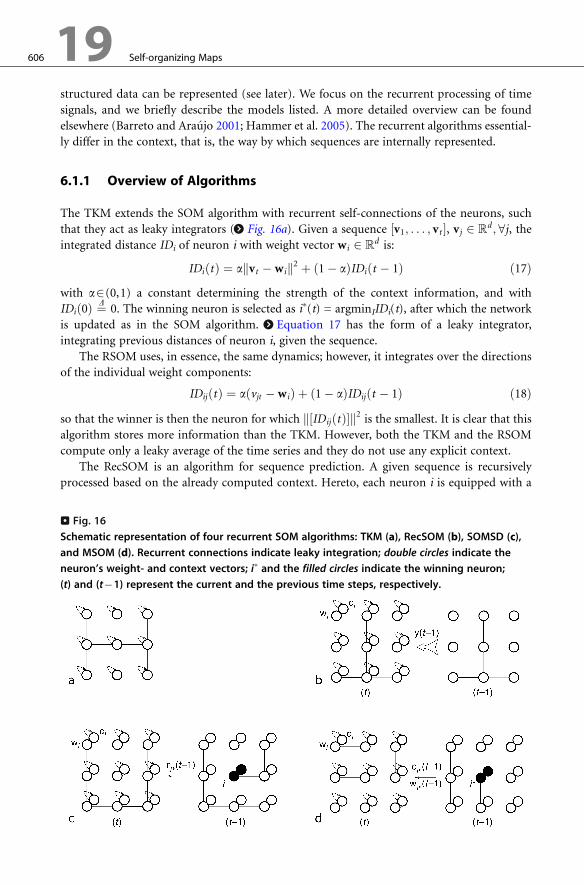
. Fig. 16

Schematic representation of four recurrent SOM algorithms: TKM (a), RecSOM (b), SOMSD (c),

and MSOM (d). Recurrent connections indicate leaky integration; double circles indicate the

neuron’s weight- and context vectors; i� and the filled circles indicate the winning neuron;

(t) and (t�1) represent the current and the previous time steps, respectively.


weight and, additionally, a context vector ci 2 N that stores an activation profile of the whole

map, indicating in which context the weight vector should arise (> Fig. 16b). The integrated

distance is defined as:

IDiðtÞ ¼ akvt � wik2 þ bkyðt � 1Þ � cik2 ð19Þwith yðt � 1Þ ¼ ½expð�ID1ðt � 1ÞÞ; . . . ; expð�IDN ðt � 1ÞÞ�, a, b> 0 constants to control the

respective contributions from pattern and context matching, and with IDið0Þ ¼D 0. The winner

is defined as the neuron for which the integrated distance is minimal. The equation contains

the exponential function in order to avoid numerical explosion: otherwise, the activation, IDi,

could become too large because the distances with respect to the contexts of all N neurons

could accumulate. Learning is performed on the weights as well as the contexts, in the usual

way (thus, involving a neighborhood function centered around the winner): the weights are

adapted toward the current input sequences, the contexts toward the recursively computed

contexts y.

The SOMSD was developed for processing labeled trees with fixed fan-out k. The limiting

case of k = 1 covers sequences. We further restrict ourselves to sequences. Each neuron has,

besides a weight, a context vector ci 2 dA, with dA the dimensionality of the lattice. The

winning neuron i� for a training input at time t is defined as (> Fig. 16c):

i� ¼ argmin akvt � wik2 þ ð1� aÞkri� ðt � 1Þ � cik2 ð20Þwith ri� the lattice coordinate of the winning neuron. The weights wi are moved in the

direction of the current input, as usual (i.e., with a neighborhood), and the contexts ci in

the direction of the lattice coordinates with the winning neuron of the previous time step (also

with a neighborhood).

The MSOM algorithm accounts for the temporal context by an explicit vector attached to

each neuron that stores the preferred context of that neuron (> Fig. 16d). The MSOM

characterizes the context by a ‘‘merging’’ of the weight and the context of the winner in the

previous time step (whence the algorithm’s name: merge SOM). The integrated distance is

defined as:

IDiðtÞ ¼ akwi � vtk2 þ ð1� aÞkci � Ctk2 ð21Þwith ci 2 d , and with Ct the expected (merged) weight/context vector, that is, the context of

the previous winner:

Ct ¼ gci� ðt � 1Þ þ ð1� gÞwi� ðt � 1Þ ð22Þwith C0 ¼D 0. Updating of wi and ci are then done in the usual SOM way, thus, with a

neighborhood function centered around the winner. The parameter, a, is controlled so as to

maximize the entropy of the neural activity.

6.1.2 Comparison of Algorithms

Hammer and coworkers (2004) pointed out that several of the mentioned recurrent self-

organizing map algorithms share their principled dynamics, but differ in their internal

representations of context. In all cases, the context is extracted as the relevant part of the

activation of the map in the previous time step. The notion of ‘‘relevance’’ thus differs between

the algorithms (see also Hammer et al. 2005). The recurrent self-organizing algorithms can be


divided into two categories: the representation of the context in the data space, such as for the

TKM andMSOM, and in a space that is related to the neurons, as for SOMSD and RecSOM. In

the first case, the storage capacity is restricted by the input dimensionality. In the latter case, it

can be enlarged simply by adding more neurons to the lattice. Furthermore, there are essential

differences in the dynamics of the algorithms. The TKM does not converge to the optimal

weights; RSOM does it but the parameter a occurs both in the encoding formula and in the

dynamics. In the MSOM algorithm, they can be controlled separately. Finally, the algorithms

differ in memory and computational complexity (RecSOM is quite demanding, SOMSD is

fast, and MSOM is somewhere in the middle), the possibility to apply different lattice types

(such as hyperbolic lattices; Ritter 1998), and their capacities (MSOM and SOMSD achieve the

capacity of finite state automata, but TKM and RSOM have smaller capacities; RecSOM is

more complex to judge).

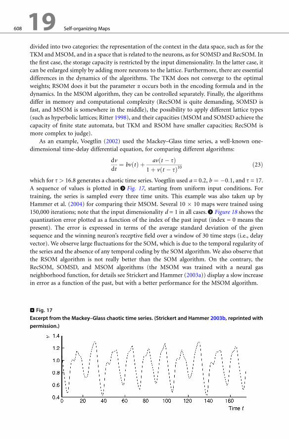
As an example, Voegtlin (2002) used the Mackey–Glass time series, a well-known one-

dimensional time-delay differential equation, for comparing different algorithms:

dv

dt¼ bvðtÞ þ avðt � tÞ

1þ vðt � tÞ10 ð23Þ

which for t> 16.8 generates a chaotic time series. Voegtlin used a = 0.2, b ¼ �0:1, and t = 17.

A sequence of values is plotted in > Fig. 17, starting from uniform input conditions. For

training, the series is sampled every three time units. This example was also taken up by

Hammer et al. (2004) for comparing their MSOM. Several 10 � 10 maps were trained using

150,000 iterations; note that the input dimensionality d = 1 in all cases. > Figure 18 shows the

quantization error plotted as a function of the index of the past input (index = 0 means the

present). The error is expressed in terms of the average standard deviation of the given

sequence and the winning neuron’s receptive field over a window of 30 time steps (i.e., delay

vector). We observe large fluctuations for the SOM, which is due to the temporal regularity of

the series and the absence of any temporal coding by the SOM algorithm. We also observe that

the RSOM algorithm is not really better than the SOM algorithm. On the contrary, the

RecSOM, SOMSD, and MSOM algorithms (the MSOM was trained with a neural gas

neighborhood function, for details see Strickert and Hammer (2003a)) display a slow increase

in error as a function of the past, but with a better performance for the MSOM algorithm.

. Fig. 17

Excerpt from the Mackey–Glass chaotic time series. (Strickert and Hammer 2003b, reprinted with

permission.)

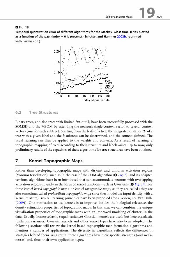
. Fig. 18

Temporal quantization error of different algorithms for the Mackey–Glass time series plotted

as a function of the past (index = 0 is present). (Strickert and Hammer 2003b, reprinted

with permission.)


6.2 Tree Structures

Binary trees, and also trees with limited fan-out k, have been successfully processed with the

SOMSD and the MSOM by extending the neuron’s single context vector to several context

vectors (one for each subtree). Starting from the leafs of a tree, the integrated distance ID of a

tree with a given label and the k subtrees can be determined, and the context defined. The

usual learning can then be applied to the weights and contexts. As a result of learning, a

topographic mapping of trees according to their structure and labels arises. Up to now, only

preliminary results of the capacities of these algorithms for tree structures have been obtained.

7 Kernel Topographic Maps

Rather than developing topographic maps with disjoint and uniform activation regions

(Voronoi tessellation), such as in the case of the SOM algorithm (> Fig. 5), and its adapted

versions, algorithms have been introduced that can accommodate neurons with overlapping

activation regions, usually in the form of kernel functions, such as Gaussians (> Fig. 19). For

these kernel-based topographic maps, or kernel topographic maps, as they are called (they are

also sometimes called probabilistic topographic maps since they model the input density with a

kernel mixture), several learning principles have been proposed (for a review, see Van Hulle

(2009)). One motivation to use kernels is to improve, besides the biological relevance, the

density estimation properties of topographic maps. In this way, we can combine the unique

visualization properties of topographic maps with an improved modeling of clusters in the

data. Usually, homoscedastic (equal variance) Gaussian kernels are used, but heteroscedastic

(differing variances) Gaussian kernels and other kernel types have also been adopted. The

following sections will review the kernel-based topographic map formation algorithms and

mention a number of applications. The diversity in algorithms reflects the differences in

strategies behind them. As a result, these algorithms have their specific strengths (and weak-

nesses) and, thus, their own application types.

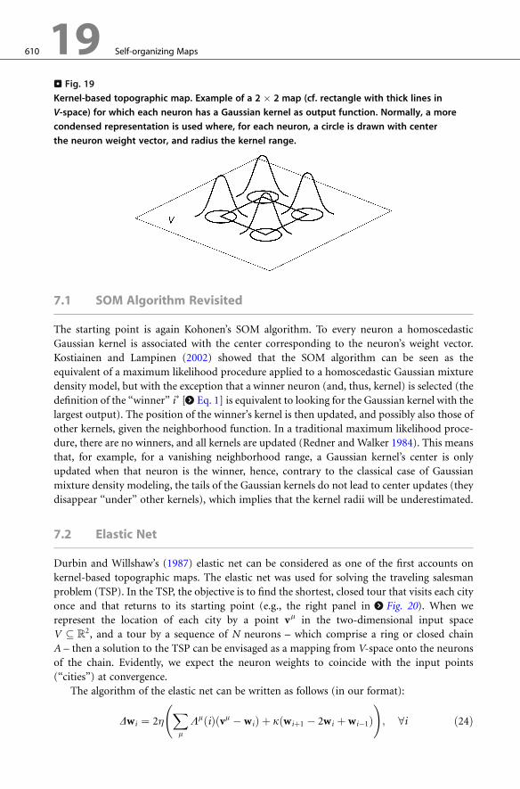
. Fig. 19

Kernel-based topographic map. Example of a 2 � 2 map (cf. rectangle with thick lines in

V-space) for which each neuron has a Gaussian kernel as output function. Normally, a more

condensed representation is used where, for each neuron, a circle is drawn with center

the neuron weight vector, and radius the kernel range.


7.1 SOM Algorithm Revisited

The starting point is again Kohonen’s SOM algorithm. To every neuron a homoscedastic

Gaussian kernel is associated with the center corresponding to the neuron’s weight vector.

Kostiainen and Lampinen (2002) showed that the SOM algorithm can be seen as the

equivalent of a maximum likelihood procedure applied to a homoscedastic Gaussian mixture

density model, but with the exception that a winner neuron (and, thus, kernel) is selected (the

definition of the ‘‘winner’’ i� [> Eq. 1] is equivalent to looking for the Gaussian kernel with the

largest output). The position of the winner’s kernel is then updated, and possibly also those of

other kernels, given the neighborhood function. In a traditional maximum likelihood proce-

dure, there are no winners, and all kernels are updated (Redner and Walker 1984). This means

that, for example, for a vanishing neighborhood range, a Gaussian kernel’s center is only

updated when that neuron is the winner, hence, contrary to the classical case of Gaussian

mixture density modeling, the tails of the Gaussian kernels do not lead to center updates (they

disappear ‘‘under’’ other kernels), which implies that the kernel radii will be underestimated.

7.2 Elastic Net

Durbin and Willshaw’s (1987) elastic net can be considered as one of the first accounts on

kernel-based topographic maps. The elastic net was used for solving the traveling salesman

problem (TSP). In the TSP, the objective is to find the shortest, closed tour that visits each city

once and that returns to its starting point (e.g., the right panel in > Fig. 20). When we

represent the location of each city by a point vm in the two-dimensional input space

V � 2, and a tour by a sequence of N neurons – which comprise a ring or closed chain

A – then a solution to the TSP can be envisaged as a mapping from V-space onto the neurons

of the chain. Evidently, we expect the neuron weights to coincide with the input points

(‘‘cities’’) at convergence.

The algorithm of the elastic net can be written as follows (in our format):

Dwi ¼ 2�Xm

LmðiÞðvm � wiÞ þ kðwiþ1 � 2wi þ wi�1Þ !

; 8i ð24Þ

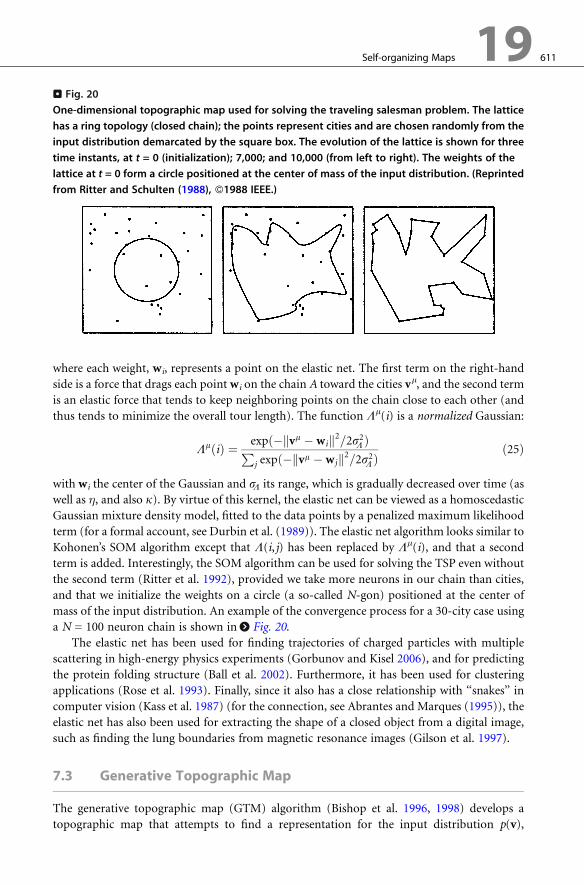
. Fig. 20

One-dimensional topographic map used for solving the traveling salesman problem. The lattice

has a ring topology (closed chain); the points represent cities and are chosen randomly from the

input distribution demarcated by the square box. The evolution of the lattice is shown for three

time instants, at t = 0 (initialization); 7,000; and 10,000 (from left to right). The weights of the

lattice at t = 0 form a circle positioned at the center of mass of the input distribution. (Reprinted

from Ritter and Schulten (1988), �1988 IEEE.)


where each weight, wi, represents a point on the elastic net. The first term on the right-hand

side is a force that drags each point wi on the chain A toward the cities vm, and the second term

is an elastic force that tends to keep neighboring points on the chain close to each other (and

thus tends to minimize the overall tour length). The function Lm(i) is a normalized Gaussian:

LmðiÞ ¼ expð�kvm � wik2=2s2L ÞPj expð�kvm � wjk2=2s2L Þ

ð25Þ

with wi the center of the Gaussian and sL its range, which is gradually decreased over time (as

well as �, and also k). By virtue of this kernel, the elastic net can be viewed as a homoscedastic

Gaussian mixture density model, fitted to the data points by a penalized maximum likelihood

term (for a formal account, see Durbin et al. (1989)). The elastic net algorithm looks similar to

Kohonen’s SOM algorithm except that L(i, j) has been replaced by Lm(i), and that a second

term is added. Interestingly, the SOM algorithm can be used for solving the TSP even without

the second term (Ritter et al. 1992), provided we take more neurons in our chain than cities,

and that we initialize the weights on a circle (a so-called N-gon) positioned at the center of

mass of the input distribution. An example of the convergence process for a 30-city case using

a N = 100 neuron chain is shown in > Fig. 20.

The elastic net has been used for finding trajectories of charged particles with multiple

scattering in high-energy physics experiments (Gorbunov and Kisel 2006), and for predicting

the protein folding structure (Ball et al. 2002). Furthermore, it has been used for clustering

applications (Rose et al. 1993). Finally, since it also has a close relationship with ‘‘snakes’’ in

computer vision (Kass et al. 1987) (for the connection, see Abrantes and Marques (1995)), the

elastic net has also been used for extracting the shape of a closed object from a digital image,

such as finding the lung boundaries from magnetic resonance images (Gilson et al. 1997).

7.3 Generative Topographic Map

The generative topographic map (GTM) algorithm (Bishop et al. 1996, 1998) develops a

topographic map that attempts to find a representation for the input distribution p(v),


v ¼ ½v1; . . . ; vd �, v 2 V , in terms of a number L of latent variables x ¼ ½x1; . . . ; xL�. This isachieved by considering a nonlinear transformation y(x,W), governed by a set of parameters

W, which maps points in the latent variable space to the input space, much the same way as the

lattice nodes in the SOM relate to positions in V-space (inverse mappingC in > Fig. 2). If one

defines a probability distribution, p(x), on the latent variable space, then this will induce a

corresponding distribution, p(y jW), in the input space.

As a specific form of p(x), Bishop and coworkers take a discrete distribution consisting of a

sum of delta functions located at the N nodes of a regular lattice:

pðxÞ ¼ 1

N

XNi¼ 1

dðx � xiÞ ð26Þ

The dimensionality, L, of the latent variable space is typically less than the dimensionality, d, of

the input space so that the transformation, y, specifies an L-dimensional manifold in V -space.

Since L<d, the distribution in V-space is confined to this manifold and, hence, is singular. In

order to avoid this, Bishop and coworkers introduced a noise model in V-space, namely, a set

of radially symmetric Gaussian kernels centered at the positions of the lattice nodes in V-space.

The probability distribution in V-space can then be written as follows:

pðvjW; sÞ ¼ 1

N

XNi¼ 1

pðvjxi;W; sÞ ð27Þ

which is a homoscedastic Gaussian mixture model. In fact, this distribution is a constrained

Gaussian mixture model since the centers of the Gaussians cannot move independently from

each other but are related through the transformation, y. Moreover, when the transformation

is smooth and continuous, the centers of the Gaussians will be topographically ordered by

construction. Hence, the topographic nature of the map is an intrinsic feature of the latent

variable model and is not dependent on the details of the learning process. Finally, the

parameters W and s are determined by maximizing the log-likelihood:

lnlðW; sÞ ¼ lnYMm¼ 1

pðvmjW; sÞ ð28Þ

and which can be achieved through the use of an expectation-maximization (EM) procedure

(Dempster et al. 1977). Because a single two-dimensional visualization plot may not be

sufficient to capture all of the interesting aspects of complex data sets, a hierarchical version

of the GTM has also been developed (Tino and Nabney 2002).

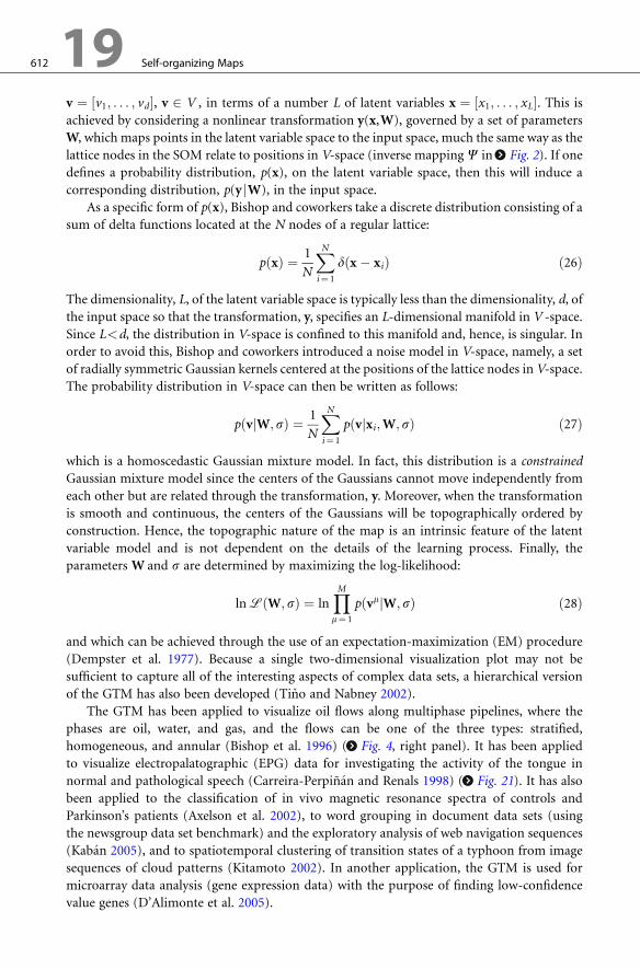
The GTM has been applied to visualize oil flows along multiphase pipelines, where the

phases are oil, water, and gas, and the flows can be one of the three types: stratified,

homogeneous, and annular (Bishop et al. 1996) (> Fig. 4, right panel). It has been applied

to visualize electropalatographic (EPG) data for investigating the activity of the tongue in

normal and pathological speech (Carreira-Perpinan and Renals 1998) (> Fig. 21). It has also

been applied to the classification of in vivo magnetic resonance spectra of controls and

Parkinson’s patients (Axelson et al. 2002), to word grouping in document data sets (using

the newsgroup data set benchmark) and the exploratory analysis of web navigation sequences

(Kaban 2005), and to spatiotemporal clustering of transition states of a typhoon from image

sequences of cloud patterns (Kitamoto 2002). In another application, the GTM is used for

microarray data analysis (gene expression data) with the purpose of finding low-confidence

value genes (D’Alimonte et al. 2005).

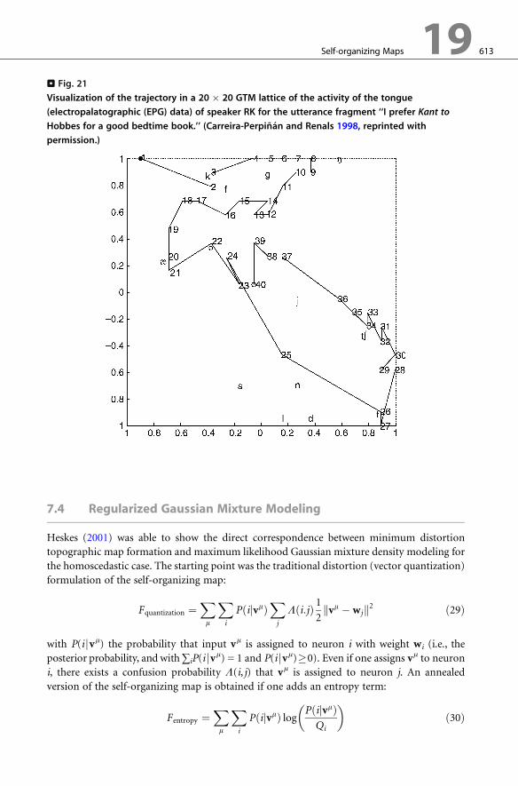
. Fig. 21

Visualization of the trajectory in a 20 � 20 GTM lattice of the activity of the tongue

(electropalatographic (EPG) data) of speaker RK for the utterance fragment ‘‘I prefer Kant to

Hobbes for a good bedtime book.’’ (Carreira-Perpinan and Renals 1998, reprinted with

permission.)


7.4 Regularized Gaussian Mixture Modeling

Heskes (2001) was able to show the direct correspondence between minimum distortion

topographic map formation and maximum likelihood Gaussian mixture density modeling for

the homoscedastic case. The starting point was the traditional distortion (vector quantization)

formulation of the self-organizing map:

Fquantization ¼Xm

Xi

PðijvmÞXj

Lði:jÞ 12kvm � wjk2 ð29Þ

with P(i jvm) the probability that input vm is assigned to neuron i with weight wi (i.e., the

posterior probability, and with∑iP(i jvm) = 1 and P(i jvm)0). Even if one assigns vm to neuron

i, there exists a confusion probability L(i, j) that vm is assigned to neuron j. An annealed

version of the self-organizing map is obtained if one adds an entropy term:

Fentropy ¼Xm

Xi

PðijvmÞ log PðijvmÞQi

� �ð30Þ


withQi the prior probability (the usual choice isQi ¼ 1N, withN the number of neurons in the

lattice. The final (free) energy is now:

F ¼ bFquantization þ Fentropy ð31Þwith b playing the role of an inverse temperature. This formulation is very convenient for an

EM procedure. The expectation step leads to:

PðijvmÞ ¼Qi exp � b

2

Pj Lði; jÞ kvm � wjk

� �P

s Qs exp � b2

Pj Lðs; jÞ kvm � wjk

� � ð32Þ

and the maximization step to:

wi ¼P

m

Pj PðjjvmÞLðj; iÞvmP

m

Pj PðjjvmÞLðj; iÞ

ð33Þ

which is also the result reached by Graepel and coworkers (1998) for the soft topographic

vector quantization (STVQ) algorithm (see the next section). Plugging (> Eq. 32) into

(> Eq. 31) leads to an error function, which allows for the connection with a maximum

likelihood procedure, for a mixture of homoscedastic Gaussians, when the neighborhood

range vanishes (L(i, j) = dij). When the neighborhood is present, Heskes showed that this leads

to a term added to the original likelihood.

As an application, Heskes considers market basket analysis. Given are a list of transactions

corresponding to the joint set of products purchased by a customer at a given time. The goal of

the analysis is tomap the products onto a two-dimensional map (lattice) such that neighboring

products are ‘‘similar.’’ Similar products should have similar conditional probabilities of buying

other products. In another application, he considers the case of transactions in a supermarket.

The products are summarized in product groups, and the co-occurrence frequencies are given.

The result is a two-dimensional density map showing clusters of products that belong together,

for example, a large cluster of household products (> Fig. 22).

7.5 Soft Topographic Vector Quantization

Another approach that considers topographic map formation as an optimization problem is

the one introduced by Klaus Obermayer and coworkers (Graepel et al. 1997,1998). They start

from the following cost function:

EðWÞ ¼ 1

2

Xm

Xi

cm;iXj

Lði; jÞ kvm � wjk2 ð34Þ

with cm,i 2 {0, 1} and for which cm,i = 1 if vm is assigned to neuron i, else cm,i = 0 (∑icm,i = 1); the

neighborhood function obeys ∑jL(i, j) = 1. The wi, 8i, for which this function is minimal, are

the optimal ones. However, the optimization is a difficult task, because it depends both on

binary and continuous variables and has many local minima. To avoid this, a technique known

as deterministic annealing is applied: the optimization is done on a smooth function para-

metrized by a parameter b, the so-called free energy. When b is small, the function is smooth

and only one global minimum remains; when large, more of the structure of the original cost

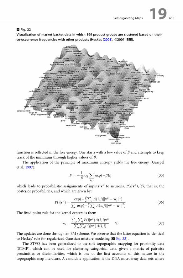
. Fig. 22

Visualization of market basket data in which 199 product groups are clustered based on their

co-occurrence frequencies with other products (Heskes (2001), �2001 IEEE).


function is reflected in the free energy. One starts with a low value of b and attempts to keep

track of the minimum through higher values of b.The application of the principle of maximum entropy yields the free energy (Graepel

et al. 1997):

F ¼ � 1

blogXcm;i

expð�bEÞ ð35Þ

which leads to probabilistic assignments of inputs vm to neurons, P(i jvm), 8i, that is, theposterior probabilities, and which are given by:

PðijvmÞ ¼ expð� b2

Pj Lði; jÞkvm � wjk2ÞP

s expð� b2

Pj Lðs; jÞkvm � wjk2Þ

ð36Þ

The fixed point rule for the kernel centers is then:

wi ¼P

m

Pj PðjjvmÞLðj; iÞvmP

m

PjPðjjvmÞLðj; iÞ

; 8i ð37Þ

The updates are done through an EM scheme. We observe that the latter equation is identical

to Heskes’ rule for regularized Gaussian mixture modeling (> Eq. 33).

The STVQ has been generalized to the soft topographic mapping for proximity data

(STMP), which can be used for clustering categorical data, given a matrix of pairwise

proximities or dissimilarities, which is one of the first accounts of this nature in the

topographic map literature. A candidate application is the DNA microarray data sets where


the data can be described by matrices with the columns representing tissue samples and the

rows genes, and the entries in the matrix correspond to the strength of the gene expression. In

Seo and Obermayer (2004), a modified version of the STMP is used for clustering documents

(‘‘document map’’).

7.6 Heteroscedastic Gaussian Kernel Topographic Map Formation

In the literature, only few approaches exist that consider heteroscedastic kernels, perhaps

because the kernel radius in the homoscedastic case is often used in an annealing schedule, as

shown above in the STVQ and the elastic net algorithms. When using heteroscedastic kernels,

a better density estimate is expected. Several algorithms for heteroscedastic kernels have been

developed (for a review, see Van Hulle (2009)). We briefly mention a few here.

Bearing in mind what was said earlier about the SOM in connection to Gaussian mixture

modeling, one can extend the original batch map, >Eq. 5, to the heteroscedastic case (Van

Hulle 2009):

wi ¼P

m Lði�; iÞvmPm Lði�; iÞ

s2i ¼P

m Lði�; iÞkv � wik2=dPm Lði�; iÞ

; 8ið38Þ

with i� = argmaxiKi (which is no longer equivalent to i� ¼ argminikv � wik, but which is

required since we now have heteroscedastic kernels), that is, an activity-based definition of

‘‘winner-takes-all,’’ rather than a minimum Euclidean distance-based one. Notice again that, by

the definition of the winner, the tails of the kernels are cut off, since the kernels overlap.

Recently we introduced (Van Hulle 2005a) a learning algorithm for kernel-based topo-

graphic map formation of heteroscedastic Gaussian mixtures that allows for a unified account

of distortion error (vector quantization), log-likelihood and Kullback–Leibler divergence, and

that generalizes Heskes’ (2001) algorithm to the heteroscedastic case.

There is also the heuristic approach suggested by Yin and Allinson (2001), which is

minimizing the Kullback–Leibler divergence, based on an idea introduced by Benaim and

Tomasini (1991), for the homoscedastic case. Albeit these authors only suggested an incre-

mental, gradient-based learning procedure (thus, with a learning rate), we can cast their

format into a fixed point learning scheme:

wi ¼P

m Lði�; iÞPðijvmÞvmPm Lði�; iÞPðijvmÞ

s2i ¼P

m Lði�; iÞPðijvmÞkvm � wik2=dPm Lði�; iÞPðijvmÞ

ð39Þ

with the winner neuron defined as i� = argmaxiP(ijvm), thus, the neuron with the largest

posterior probability.

In a still different approach, an input to lattice transformation F is considered that admits

a kernel function, a Gaussian (Van Hulle 2002a) hF(v),F(wi)i = K(v,wi,si):

K ðv;wi; siÞ ¼ exp �kv � wik22s2i

!ð40Þ


When performing topographic map formation, we require that the weight vectors are

updated, so as to minimize the expected value of the squared Euclidean distance kv � wik2and, hence, following our transformation F, we instead wish to minimize kFðvÞ � FðwiÞk2,which we will achieve by performing gradient descent with respect to wi. The leads to the

following fixed point rules to which we have added a neighborhood function:

wi ¼P

m Lði; i�ÞK ðvm;wi; siÞvmPm Lði; i�ÞKðvm;wi; siÞ

s2i ¼1

rd

Pm Lði; i�ÞK ðvm;wi; siÞkvm � wik2P

m Lði; i�ÞK ðvm;wi; siÞ

ð41Þ

with r a scale factor (a constant) designed to relax the local Gaussian (and d large) assumption

in practice, and with i� ¼ argmax8i2A Kðv;wi; siÞ.Rather than having a real-valued neural activation, one could also threshold the kernel into

a binary variable: in the kernel-based maximum entropy rule (kMER), a neuron, i, is activated

by input v when kwi � vk < si , where si is the kernel radius of neuron i, and which defines a

hyperspherical activation region, Si (Van Hulle 1998). The membership function, 1iðvÞ,equals unity when neuron i is activated by v, else it is zero. When there are no neurons active

for a given input, the neuron that is positioned closest to that input is defined active. The

incremental learning rules for the weights and radii of neuron i are as follows:

Dwi ¼ �Xj

Lði; jÞXiðvÞsignðv � wiÞ

Dsi ¼ �rrN

ð1�1iðvÞÞ �1iðvÞ� � ð42Þ

with sign(.), the sign function taken component-wise, Z the learning rate, XiðvÞ ¼ 1iPj1j

a

fuzzy membership function, and rr ¼ rNN�r . It can be shown that the kernel ranges converge to

the case where the average probabilities become equal, h1ii ¼ rN; 8i. By virtue of the latter,

kMER is said to generate an equiprobabilistic topographic map (which avoids dead units). The

algorithm has been considered for a wide range of applications, such as shape clustering (Van

Hulle and Gautama 2004), music signal clustering (Van Hulle 2000), and the linking of patent

and scientific publication databases (Deleus and Van Hulle 2001). More recently, a fixed point

version, called batch map kMER, was introduced (Gautama and Van Hulle 2006), and applied

to handwritten numerals clustering.

7.7 Kernels Other Than Gaussians

In principle, kernels other than Gaussians could be used in topographic map formation. For

example, Heskes pointed out that his regularized mixture modeling approach could, in

principle, accommodate any kernel of the exponential family, such as the gamma, multino-

mial, and the Poisson distributions (Heskes 2001).

In another case, the kernel is considered for which the differential entropy of the kernel

output will be maximal given a Gaussian input, that is, the incomplete gamma distribution

kernel (Van Hulle 2002b).

Another type of kernel is the Edgeworth-expanded Gaussian kernel, which consists of a

Gaussian kernel multiplied by a series of Hermite polynomials of increasing order, and of which

the coefficients are specified by (the second- and higher-order) cumulants (Van Hulle 2005b).


In still another case, a mixture of Bernoulli distributions is taken (Verbeek et al. 2005) for

the specific purpose to better encode binary data (e.g., word occurrence in a document). This also

leads to an EM algorithm for updating the posteriors, as well as the expected joint log-likelihood

with respect to the parameters of the Bernoulli distributions. However, as the posteriors become

quite peaked for higher dimensions, for visualization purposes, a power function of them was

chosen. Several applications have been demonstrated, including word grouping in document

data sets (newsgroup data set) and credit data analysis (from the University of California, Irvine

(UCI) machine learning repository http://archive.ics.uci.edu/ml/).

7.8 Future Developments

An expected development is to go beyond the limitation of the current kernel-based

topographic maps that the inputs need to be vectors (we already saw the extension toward

categorical data). But in the area of structural pattern recognition, more powerful data

structures can be processed, such as strings, trees, and graphs. The SOM algorithm has

already been extended toward strings (Kohonen and Somervuo 1998) and graphs, which

include strings and trees (Gunter and Bunke 2002; Seo and Obermayer 2004; Steil and

Sperduti 2007) (see also the SOMSD and the MSOM algorithms above). However, new

types of kernels for strings, trees, and graphs have been suggested in the support vector

machine literature (thus, outside the topographic map literature) (for reviews, see Shawe-

Taylor and Cristianini (2004) and Jin et al. (2005)). The integration of these new types of

kernels into kernel-based topographic maps is yet to be done, but could turn out to be a

promising evolution for biochemical applications, such as visualizing and clustering sets of

structure-based molecule descriptions.

8 Conclusion

In this chapter we introduced the self-organizing map (SOM) algorithm, discussed its proper-

ties, limitations, and types of application, and reviewed a number of extensions and other

types of topographic map formation algorithms, such as the growing, the recurrent, and the

kernel topographic maps. We also indicated how recent developments in topographic maps

enable us to consider categorical data, time series, and tree-structured data, widening further

the application field toward microarray data analysis, document analysis and retrieval, explor-

atory analysis of web navigation sequences, and the visualization of protein structures and

long DNA sequences.

Acknowledgments

The author is supported by the Excellence Financing program (EF 2005) and the CREA

Financing program (CREA/07/027) of K.U.Leuven, the Belgian Fund for Scientific Research –

Flanders (G.0234.04 and G.0588.09), the Flemish Regional Ministry of Education (Belgium)

(GOA 2000/11), the Belgian Science Policy (IUAP P6/29), and the European Commission

(NEST-2003-012963, STREP-2002-016276, IST-2004-027017, and ICT-2007-217077).


References

Abrantes AJ, Marques JS (1995) Unified approach to

snakes, elastic nets, and Kohonen maps. In: Proceed-

ings of the IEEE International Conference on Acous-

tics, Speech and Signal Processing (ICASSP’95).

IEEE Computer Society, Los Alamitos, CA, vol 5,

pp 3427–3430

Ahalt SC, Krishnamurthy AK, Chen P, Melton DE (1990)

Competitive learning algorithms for vector quanti-

zation. Neural Netw 3:277–290

Alahakoon D, Halgamuge SK, Srinivasan B (2000)

Dynamic self organising maps with controlled

growth for knowledge discovery. IEEE Trans Neural

Netw (Special issue on knowledge discovery and

data mining) 11(3):601–614

Axelson D, Bakken IJ, Gribbestad IS, Ehrnholm B, Nilsen

G, Aasly J (2002) Applications of neural network

analyses to in vivo 1H magnetic resonance spectros-

copy of Parkinson disease patients. J Magn Reson

Imaging 16(1):13–20

Ball KD, Erman B, Dill KA (2002) The elastic

net algorithm and protein structure prediction.

J Comput Chem 23(1):77–83

Barreto G, Araujo A (2001) Time in self-organizing

maps: an overview of models. Int J Comput Res

10(2):139–179

Bauer H-U, Villmann T (1997) Growing a hypercubical

output space in a self-organizing feature map. IEEE

Trans Neural Netw 8(2):218–226

Bauer H-U, Der R, Herrmann M (1996) Controlling the

magnification factor of self-organizing feature maps.

Neural Comput 8:757–771

Benaim M, Tomasini L (1991) Competitive and self-

organizing algorithms based on the minimization

of an information criterion. In: Proceedings of

1991 international conference in artificial neural

networks (ICANN’91). Espoo, Finland. Elsevier Sci-

ence Publishers, North-Holland, pp 391–396

Bishop CM (2006) Pattern recognition and machine

learning. Springer, New York

Bishop CM, Svensen M, Williams CKI (1996) GTM: a

principled alternative to the self-organizing map. In:

Proceedings 1996 International Conference on Arti-

ficial Neural Networks (ICANN’96). Bochum,

Germany, 16–19 July 1996. Lecture notes in com-

puter science, vol 1112. Springer, pp 165–170

Bishop CM, Hinton GE, and Strachan IGD (1997) In:

Proceedings IEE fifth international conference on

artificial neural networks. Cambridge UK, 7–9 July

1997, pp 111–116

Bishop CM, Svensen M, Williams CKI (1998) GTM: the

generative topographic mapping. Neural Comput

10:215–234

Blackmore J, Miikkulainen R (1993) Incremental grid

growing: encoding high-dimensional structure into

a two-dimensional feature map. In: Proceedings of

IEEE international conference on neural networks.

San Francisco, CA. IEEE Press, Piscataway, NJ, vol 1,

pp 450–455

Bruske J, Sommer G (1995) Dynamic cell structure learns

perfectly topology preserving map. Neural Comput

7(4):845–865

Carreira-Perpinan MA, Renals S (1998) Dimensionality

reduction of electropalatographic data using latent

variable models. Speech Commun 26(4):259–282

Centre NNR (2003) Bibliography on the Self-Organizing

Map (SOM) andLearningVectorQuantization (LVQ),

Helsinki University of Technology. http://liinwww.ira.

uka.de/bibliography/Neural/SOM.LVQ.html

Chappell G, Taylor J (1993) The temporal Kohonen map.

Neural Netw 6:441–445

Chinrungrueng C, Sequin CH (1995) Optimal

adaptive k-means algorithm with dynamic adjust-

ment of learning rate. IEEE Trans Neural Netw

6:157–169

Cottrell M, Fort JC (1987) Etude d’un processus d’auto-

organization. Ann Inst Henri Poincare 23:1–20

D’Alimonte D, Lowe D, Nabney IT, Sivaraksa M (2005)

Visualising uncertain data. In: Proceedings Europe-

an conference on emergent aspects in clinical data

analysis (EACDA2005). Pisa, Italy, 28–30 September

2005. http://ciml.di.unipi.it/EACDA2005/papers.

html

Deleus FF, Van Hulle MM (2001) Science and technology

interactions discovered with a new topographic

map-based visualization tool. In: Proceedings of

7th ACM SIGKDD international conference on

knowledge discovery in data mining. San Francisco,

26–29 August 2001. ACM Press, New York, pp 42–50

Dempster AP, Laird NM, Rubin DB (1977) Maximum

likelihood for incomplete data via the EM algo-

rithm. J R Stat Soc B 39:1–38

Der R, Herrmann M (1993) Phase transitions in self-

organizing feature maps. In: Proceedings of 1993

international conference on artificial neuron net-

works (ICANN’93). Amsterdam, The Netherlands,

13–16 September 1993, Springer, New York,

pp 597–600

DeSieno D (1988) Adding a conscience to competitive

learning. In: Proceedings of IEEE international con-

ference on neural networks. San Diego, CA, IEEE

Press, New York, vol I, pp 117–124

Durbin R, Willshaw D (1987) An analogue approach to

the travelling salesman problem using an elastic net

method. Nature 326:689–691


Durbin R, Szeliski R, Yuille AL (1989) An analysis of the

elastic net approach to the traveling salesman prob-

lem. Neural Comput 1:348–358

Erwin E, Obermayer K, Schulten K (1992) Self-

organizing maps: ordering, convergence properties

and energy functions. Biol Cybern 67:47–55

Euliano NR, Principe JC (1999). A spatiotemporal mem-

ory based on SOMs with activity diffusion. In:

Oja E, Kaski S (eds) Kohonen maps. Elsevier,

Amsterdam, The Netherlands, pp 253–266

Fritzke B (1994) Growing cell structures – a self-organizing

network for unsupervised and supervised learning.

Neural Netw 7(9):1441–1460

Fritzke B (1995a) A growing neural gas network learns

topologies. In: Tesauro G, Touretzky DS, Leen TK

(eds) Advances in neural information proceedings

systems 7 (NIPS 1994). MIT Press, Cambridge, MA,

pp 625–632

Fritzke B (1995b) Growing grid – a self-organizing net-

work with constant neighborhood range and adap-

tation strength. Neural Process Lett 2(5):9–13

Fritzke B (1996) Growing self-organizing networks –

why? In: European symposium on artificial

neural networks (ESANN96). Bruges, Belgium,

1996. D Facto Publications, Brussels, Belgium,

pp 61–72

Gautama T, Van Hulle MM (2006) Batch map extensions

of the kernel-based maximum entropy learning rule.

IEEE Trans Neural Netw 16(2):529–532

Gersho A, Gray RM (1991) Vector quantization and

signal compression. Kluwer, Boston, MA/Dordrecht

Geszti T (1990) Physical models of neural networks.

World Scientific Press, Singapore

Gilson SJ, Middleton I, Damper RI (1997) A

localised elastic net technique for lung boundary

extraction from magnetic resonance images. In:

Proceedings of fifth international conference on

artificial neural networks. Cambridge, UK, 7–9

July 1997. Mascarenhas Publishing, Stevenage,

UK, pp 199–204

Gorbunov S, Kisel I (2006) Elastic net for stand-alone

RICH ring finding. Nucl Instrum Methods Phys Res

A 559:139–142

Graepel T, Burger M, Obermayer K (1997) Phase transi-

tions in stochastic self-organizing maps. Phys Rev E

56(4):3876–3890

Graepel T, Burger M, Obermayer K (1998) Self-organizing

maps: generalizations and new optimization techni-

ques. Neurocomputing 21:173–190

Grossberg S (1976) Adaptive pattern classification and

universal recoding: I. Parallel development and

coding of neural feature detectors. Biol Cybern

23:121–134

Gunter S, Bunke H (2002) Self-organizing map for clus-

tering in the graph domain, Pattern Recog Lett

23:415–417

Hagenbuchner M, Sperduti A, Tsoi AC (2003) A self-

organizingmap for adaptive processing of structured

data. IEEE Trans Neural Netw 14(3):491–505

Hammer B, Micheli A, Strickert M, Sperduti A (2004)

A general framework for unsupervised processing

of structured data. Neurocomputing 57:3–35

Hammer B, Micheli A, Neubauer N, Sperduti A, Strickert

M (2005) Self organizing maps for time series.

In: Proceedings of WSOM 2005. Paris, France,

5–8 September 2005, pp 115–122

Heskes T (2001) Self-organizing maps, vector quantiza-

tion, and mixture modeling. IEEE Trans Neural

Netw 12(6):1299–1305

Heskes TM, Kappen B (1993) Error potentials for self-

organization. In: Proceedings of IEEE international

conference on neural networks. San Francisco, CA.

IEEE Press, Piscataway, NJ, pp 1219–1223

Jin B, Zhang Y-Q, Wang B (2005) Evolutionary granular

kernel trees and applications in drug activity compar-

isons, In: Proceedings of the 2005 IEEE Symposium

on Computational Intelligence in Bioinformatics and

Computational Biology (CIBCB’05). San Diego, CA,

14–15 November 2005, IEEE Press, Piscataway, NY,

pp 1–6

Kaban A (2005) A scalable generative topographic

mapping for sparse data sequences. In: Proceedings

of the International Conference on Information

Technology: Coding and Computing (ITCC’05).

Las Vegas, NV, 4–6 April 2005. IEEE Computer

Society, vol 1, pp 51–56

Kass M, Witkin A, Terzopoulos D (1987) Active contour

models. Int J Comput Vis 1(4):321–331

Kangas J (1990) Time-delayed self-organizing maps. In:

Proceedings IEEE/INNS international Joint Confer-

ence on neural networks 1990. San Diego, CA, IEEE,

New York, vol 2, pp 331–336

Kaski S, Honkela T, Lagus K, Kohonen T (1998) WEB-

SOM – self-organizing maps of document collec-

tions. Neurocomputing 21:101–117

Kim YK, Ra JB (1995) Adaptive learning method in self-

organizing map for edge preserving vector quantiza-

tion. IEEE Trans Neural Netw 6:278–280

Kitamoto A (2002) Evolution map: modeling state transi-

tion of typhoon image sequences by spatio-temporal

clustering. Lect Notes Comput Sci 2534/2002:

283–290

Kohonen T (1982) Self-organized formation of topolog-

ically correct feature maps. Biol Cybern 43:59–69

Kohonen T (1984) Self-organization and associative

memory. Springer, Heidelberg

Kohonen T (1991) Self-organizing maps: optimization

approaches. In: Kohonen T, Makisara K, Simula O,

Kangas J (eds) Artificial neural networks. North-

Holland, Amsterdam, pp 981–990

Kohonen T (1995) Self-organizing maps, 2nd edn.

Springer, Heidelberg


Kohonen T (1997) Self-organizing maps. Springer

Kohonen T, Somervuo P (1998) Self-organizing maps on

symbol strings. Neurocomputing 21:19–30

Kohonen T, Kaski S, Salojarvi J, Honkela J, Paatero V,

Saarela A (1999) Self organization of a massive doc-

ument collection. IEEE Trans Neural Netw 11(3):

574–585

Koskela T, Varsta M, Heikkonen J, Kaski K (1998) Recur-

rent SOM with local linear models in time series

prediction. In: Verleysen M (ed) Proceedings of 6th

European symposium on artificial neural networks

(ESANN 1998). Bruges, Belgium, April 22–24, 1998.

D-Facto, Brussels, Belgium, pp 167–172

Kostiainen T, Lampinen J (2002) Generative probability

density model in the self-organizing map. In: Seiffert

U, Jain L (eds) Self-organizing neural networks:

Recent advances and applications. Physica-Verlag,

Heidelberg, pp 75–94

Laaksonen J, Koskela M, Oja E (2002) PicSOM–self-

organizing image retrieval with MPEG-7 content

descriptors. IEEE Trans Neural Netw 13(4):841–853

Lin JK, Grier DG, Cowan JD (1997) Faithful representa-

tion of separable distributions. Neural Comput

9:1305–1320

Linsker R (1988) Self-organization in a perceptual net-

work. Computer 21:105–117

Linsker R (1989) How to generate ordered maps by

maximizing the mutual information between input

and output signals. Neural Comput 1:402–411

Luttrell SP (1989) Self-organization: a derivation from

first principles of a class of learning algorithms. In:

Proceedings IEEE international joint conference

on neural networks (IJCNN89). Washington, DC,

Part I, IEEE Press, Piscataway, NJ, pp 495–498

Luttrell SP (1990) Derivation of a class of training algo-

rithms. IEEE Trans Neural Netw 1:229–232

Luttrell SP (1991) Code vector density in topographic

mappings: scalar case. IEEE Trans Neural Netw

2:427–436

Martinetz TM (1993) Competitive Hebbian learning rule

forms perfectly topology preserving maps. In: Pro-

ceedings of international conference on artificial

neural networks (ICANN93). Amsterdam, The

Netherlands, 13–16 September 1993. Springer, Lon-

don, pp 427–434

Martinetz T, Schulten K (1991) A ‘‘neural-gas’’ network

learns topologies. In: Kohonen T, Makisara K,

Simula O, Kangas J (eds) Proceedings of Inter-

national Conference on Artificial Neural Networks

(ICANN-91). Espoo, Finland, 24–28 June 1991, vol I,

North-Holland, Amsterdam, The Netherlands,

pp 397–402

Martinetz T, Berkovich S, Schulten K (1993) ‘‘Neural-

gas’’ network for vector quantization and its appli-

cation to time-series prediction. IEEE Trans Neural

Netw 4(4):558–569

Merkl D, He S, Dittenbach M, Rauber A (2003)

Adaptive hierarchical incremental grid growing: an

architecture for high-dimensional data visualiza-

tion. In: Proceedings of 4th workshop on self-orga-

nizing maps (WSOM03). Kitakyushu, Japan, 11–14

September 2003

Mulier F, Cherkassky V (1995) Self-organization as an

iterative kernel smoothing process. Neural Comput

7:1165–1177

Rauber A, Merkl D, Dittenbach M (2002) The grow-

ing hierarchical self-organizing map: exploratory

analysis of high-dimensional data. IEEE Trans

Neural Netw 13(6):1331–1341

Redner RA, Walker HF (1984) Mixture densities, maxi-

mum likelihood and the EM algorithm. SIAM Rev

26(2):195–239

Risi S, Morchen F, Ultsch A, Lewark P (2007) Visual

mining in music collections with emergent SOM.

In: Proceedings of workshop on self-organizing

maps (WSOM ’07). Bielefeld, Germany, September

3–6, 2007, ISBN: 978-3-00-022473-7, CD ROM,

available online at http://biecoll.ub.uni-bielefeld.de

Ritter H (1991) Asymptotic level density for a class of

vector quantization processes. IEEE Trans Neural

Netw 2(1):173–175

Ritter H (1998) Self-organizing maps in non-Euclidean

spaces. In: Oja E, Kaski S (eds) Kohonen maps.

Elsevier, Amsterdam, pp 97–108

Ritter H, Kohonen T (1989) Self-organizing semantic

maps. Biol Cybern 61:241–254

Ritter H, Schulten K (1986) On the stationary state of

Kohonen’s self-organizing sensory mapping. Biol

Cybern 54:99–106

Ritter H, Schulten K (1988) Kohonen’s self-organizing

maps: exploring their computational capabilities, In:

Proceedings of IEEE international conference on

neural networks (ICNN). San Diego, CA. IEEE,

New York, vol I, pp 109–116

Ritter H, Martinetz T, Schulten K (1992) Neural compu-

tation and self-organizing maps: an introduction.

Addison-Wesley, Reading, MA

Rose K, Gurewitz E, Fox GC (1993) Constrained cluster-

ing as an optimization method. IEEE Trans Pattern

Anal Mach Intell 15(8):785–794

Schulz R, Reggia JA (2004) Temporally asymmetric

learning supports sequence processing in multi-

winner self-organizing maps. Neural Comput 16(3):

535–561

Seo S, Obermayer K (2004) Self-organizing maps and

clustering methods for matrix data. Neural Netw

17(8–9):1211–1229

Shawe-Taylor J, Cristianini N (2004) Kernel methods

in computational biology. MIT Press, Cambridge,

MA

Simon G, Lendasse A, Cottrell M, Fort J-C, Verleysen M

(2003) Double SOM for long-term time series


prediction. In: Proceedings of the workshop on self-

organizing maps (WSOM 2003). Hibikino, Japan,

September 11–14, 2003, pp 35–40

Somervuo PJ (2004) Online algorithm for the self-

organizing map of symbol strings. Neural Netw

17(8–9):1231–1240

Steil JJ, Sperduti A (2007) Indices to evaluate self-

organizing maps for structures. In: Proceedings of

the workshop on self-organizing maps (WSOM07)

Bielefeld, Germany, 3–6 September 2007. CD ROM,

2007, available online at http://biecoll.ub.

uni-bielefeld.de

Strickert M, Hammer B (2003a) Unsupervised recursive

sequence processing, In: Verleysen M (ed) European

Symposium on Artificial Neural Networks (ESANN

2003). Bruges, Belgium, 23–25 April 2003. D-Side

Publications, Evere, Belgium, pp 27–32

Strickert M, Hammer B (2003b) Neural gas for

sequences. In: Proceedings of the workshop on

self-organizing maps (WSOM’03). Hibikino,

Japan, September 2003, pp 53–57

Strickert M, Hammer B (2005) Merge SOM for temporal

data. Neurocomputing 64:39–72

Tino P, Nabney I (2002) Hierarchical GTM: constructing

localized non-linear projection manifolds in a prin-

cipled way. IEEE Trans Pattern Anal Mach Intell

24(5):639–656

Tino P, Kaban A, Sun Y (2004) A generative probabilistic

approach to visualizing sets of symbolic sequences.

In: Kohavi R, Gehrke J, DuMouchel W, Ghosh J

(eds) Proceedings of the tenth ACM SIGKDD inter-

national conference on knowledge discovery and

data mining (KDD-2004), Seattle, WA, 22–25 August

2004. ACM Press, New York, pp 701–706

Tolat V (1990) An analysis of Kohonen’s self-organizing

maps using a system of energy functions. Biol

Cybern 64:155–164

Ultsch A, Siemon HP (1990) Kohonen’s self organizing

feature maps for exploratory data analysis. In: Pro-

ceedings international neural networks. Kluwer,

Paris, pp 305–308

Ultsch A, Morchen F (2005) ESOM-Maps: Tools for

clustering, visualization, and classification with

emergent SOM. Technical Report No. 46, Depart-

ment of Mathematics and Computer Science, Uni-

versity of Marburg, Germany

Ueda N, Nakano R (1993) A new learning approach

based on equidistortion principle for optimal vector

quantizer design. In: Proceedings of IEEE NNSP93,

Linthicum Heights, MD. IEEE, Piscataway, NJ,

pp 362–371

Van den Bout DE, Miller TK III (1989) TInMANN:

the integer Markovian artificial neural network. In:

Proceedings of international joint conference

on neural networks (IJCNN89). Washington, DC,

18–22 June 1989, Erlbaum, Englewood Chifts, NJ,

pp II205–II211

Van Hulle MM (1997a) Topology-preserving map for-

mation achieved with a purely local unsupervised

competitive learning rule. Neural Netw 10(3):

431–446

Van Hulle MM (1997b) Nonparametric density estima-

tion and regression achieved with topographic maps

maximizing the information-theoretic entropy of

their outputs. Biol Cybern 77:49–61

Van Hulle MM (1998) Kernel-based equiprobabilistic

topographic map formation. Neural Comput

10(7):1847–1871

Van Hulle MM (2000) Faithful representations and to-

pographic maps: from distortion- to information-

based self-organization. Wiley, New York

Van Hulle MM (2002a) Kernel-based topographic map

formation by local density modeling. Neural Com-

put 14(7):1561–1573

Van Hulle MM (2002b) Joint entropy maximization in

kernel-based topographic maps. Neural Comput

14(8):1887–1906

Van Hulle MM (2005a) Maximum likelihood topograph-

ic map formation. Neural Comput 17(3):503–513

Van Hulle MM (2005b) Edgeworth-expanded topo-

graphic map formation. In: Proceedings of work-

shop on self-organizing maps (WSOM05). Paris,

France, 5–8 September 2005, pp 719–724

Van Hulle MM (2009) Kernel-based topographic maps:

theory and applications. In: Wah BW (ed) Encyclo-

pedia of computer science and engineering. Wiley,

Hoboken, vol 3, pp 1633–1650

Van Hulle MM, Gautama T (2004) Optimal smoothing

of kernel-based topographic maps with application

to density-based clustering of shapes. J VLSI

Signal Proces Syst Signal, Image, Video Technol

37:211–222

Verbeek JJ, Vlassis N, Krose BJA (2005) Self-organizing

mixture models. Neurocomputing 63:99–123

Vesanto J (1997) Using the SOM and local models in

time-series prediction. In: Proceedings of workshop

on self-organizing maps (WSOM 1997). Helsinki,

Finland, 4–6 June 1997. Helsinki University of Tech-

nology, Espoo, Finland, pp 209–214

Voegtlin T (2002) Recursive self-organizing maps.

Neural Netw 15(8–9):979–992

Wiemer JC (2003) The time-organized map algorithm:

extending the self-organizing map to spatiotempo-

ral signals. Neural Comput 15(5):1143–1171

Willshaw DJ, von der Malsburg C (1976) How patterned

neural connections can be set up by self-organiza-

tion. Proc Roy Soc Lond B 194:431–445

Yin H, Allinson NM (2001) Self-organizing mixture net-

works for probability density estimation. IEEE Trans

Neural Netw 12:405–411

handbook of natural computing || self-organizing maps

Documents