happiness in datalog
TRANSCRIPT
Happiness in Datalog
Jef Wijsen
March 20, 2019
Outline
Introduction to Datalog with Negation
Reasoning Tasks
Conjunctive Queries
Unions of Conjunctive Queries
Conjunctive Queries with Safe Atomic Negation
Datalog
Datalog with Stratified Negation
Linear Stratified Datalog
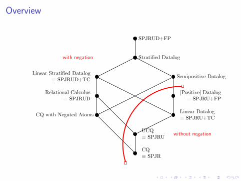
Overview
SPJRUD+FP
[Positive] Datalog≡ SPJRU+FP
Stratified Datalog
Linear Datalog≡ SPJRU+TC
Linear Stratified Datalog≡ SPJRUD+TC
UCQ≡ SPJRU
CQ≡ SPJR
Relational Calculus≡ SPJRUD
CQ with Negated Atoms
Semipositive Datalog
without negation
with negation
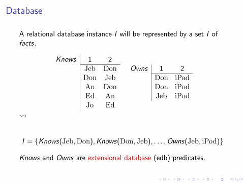
Database
A relational database instance I will be represented by a set I offacts.
Knows 1 2Jeb DonDon JebAn DonEd AnJo Ed
Owns 1 2Don iPadDon iPodJeb iPod
I = {Knows(Jeb,Don),Knows(Don, Jeb), . . . ,Owns(Jeb, iPod)}
Knows and Owns are extensional database (edb) predicates.
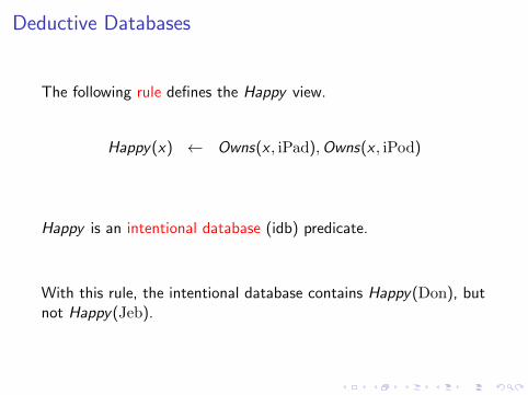
Deductive Databases
The following rule defines the Happy view.
Happy(x) ← Owns(x , iPad),Owns(x , iPod)
Happy is an intentional database (idb) predicate.
With this rule, the intentional database contains Happy(Don), butnot Happy(Jeb).

Multiple Rules
Happy(x) ← Owns(x , iPad),Owns(x , iPod)
Happy(x) ← Owns(x , iPad)
Happy(x) ← Owns(x , iPod)
With these rules, the intentional database contains Happy(Don)and Happy(Jeb).
The first rule is redundant.

Composition
Likes(x , y) ← Knows(x , y),Owns(y , iPad)
Likes(x , y) ← Knows(x , y),Owns(y , iPod)
Happy(y) ← Likes(x , y)
The first two rules state that people like every person they knowwho has an iPad or an iPod. The third rule states that you arehappy if someone likes you.With these rules, the intentional database contains, among others:
I Likes(Jeb,Don) because Jeb knows Don, and Don owns aniPad;
I Happy(Don) because Jeb likes Don.
Likes Happy
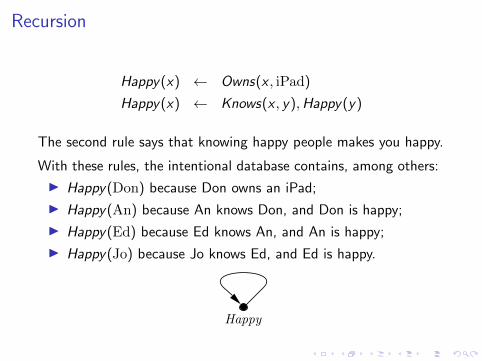
Recursion
Happy(x) ← Owns(x , iPad)
Happy(x) ← Knows(x , y),Happy(y)
The second rule says that knowing happy people makes you happy.
With these rules, the intentional database contains, among others:
I Happy(Don) because Don owns an iPad;
I Happy(An) because An knows Don, and Don is happy;
I Happy(Ed) because Ed knows An, and An is happy;
I Happy(Jo) because Jo knows Ed, and Ed is happy.
Happy

Safe negation of edb predicates
Unhappy(x) ← Knows(x , y),Owns(y , z),¬Owns(x , z)
The safety requirement states that every variable that occurs in arule, must occur positively in the body of the rule (i.e., the part ofthe rule that occurs at the right of ←).
The following two rules are not safe (so they are syntacticallyincorrect), because z occurs in the rule but z does not occurpositively in the body:
R(x , z) ← Knows(x , y)
S(x) ← Knows(x , y),¬Owns(x , z)

Safe negation of idb predicates
Unhappy(x) ← Knows(x , y),Owns(y , z),¬Owns(x , z)
Happy(x) ← Owns(x , y),¬Unhappy(x)
Unhappy Happy
−

Safe negation of idb predicates
The following program is syntactically correct but meaningless:
Unhappy(x) ← Owns(x , y),¬Happy(x)
Happy(x) ← Owns(x , y),¬Unhappy(x)
Unhappy Happy
−
−

Recursion and Negation
Person(x) ← Knows(x , y)
Person(y) ← Knows(x , y)
Person(x) ← Owns(x , y)
Happy(x) ← Owns(x , iPad)
Happy(x) ← Knows(x , y),Happy(y)
Unhappy(x) ← Person(x),¬Happy(x)
−Happy Unhappy
Person

Exercise
Get owners who own everything that can be owned.
Owner(x) ← Owns(x , y)
MissingSomething(x) ← Owner(x),Owns(u, z),¬Owns(x , z)
Answer(x) ← Owner(x),¬MissingSomething(x)
In relational calculus:
{x | ∃y (Owns(x , y) ∧ ∀u∀z (Owns(u, z)→ Owns(x , z)))}
In relational algebra (if the schema is Owns[A,B]):
πA(Owns)− πA((πA(Owns) on πB(Owns))− Owns)

Outline
Introduction to Datalog with Negation
Reasoning Tasks
Conjunctive Queries
Unions of Conjunctive Queries
Conjunctive Queries with Safe Atomic Negation
Datalog
Datalog with Stratified Negation
Linear Stratified Datalog

Questions
I Can we distinguish meaningful programs (i.e., sets of rules)from meaningless programs?
I Can we define precise semantics for all meaningful programs?
I Is there an algorithm for simplifying a given program P (i.e.,for constructing a “shorter” program that is equivalent to P)?

Containment (v) and equivalence (≡) of queries
Let q1, q2 be two queries in some query language L(e.g., L = relational calculus or L = SPJR algebra).
We write q1 ≡ q2 if for every database I ,
q1(I ) = q2(I ).
We write q1 v q2 if for every database I ,
q1(I ) ⊆ q2(I ).
Note:
I q1(I ) denotes the answer of q1 on database I ; and
I q1(~x) denotes that ~x is the sequence of free variables of q1.
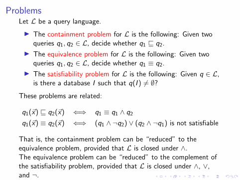
ProblemsLet L be a query language.
I The containment problem for L is the following: Given twoqueries q1, q2 ∈ L, decide whether q1 v q2.
I The equivalence problem for L is the following: Given twoqueries q1, q2 ∈ L, decide whether q1 ≡ q2.
I The satisfiability problem for L is the following: Given q ∈ L,is there a database I such that q(I ) 6= ∅?
These problems are related:
q1(~x) v q2(~x) ⇐⇒ q1 ≡ q1 ∧ q2
q1(~x) ≡ q2(~x) ⇐⇒ (q1 ∧ ¬q2) ∨ (q2 ∧ ¬q1) is not satisfiable
That is, the containment problem can be “reduced” to theequivalence problem, provided that L is closed under ∧.The equivalence problem can be “reduced” to the complement ofthe satisfiability problem, provided that L is closed under ∧, ∨,and ¬.

Undecidability
Theorem
1. The containment problem for relational calculus isundecidable.
2. The equivalence problem for relational calculus is undecidable.
3. The satisfiability problem for relational calculus is undecidable.
This is different from the undecidability of theEntscheidungsproblem [Tur36] because database instances arefinite, whereas in conventional predicate calculus, both finite andinfinite structures are considered.
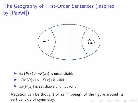
The Geography of First-Order Sentences (inspiredby [Pap94])
I ∃x (P(x) ∧ ¬P(x)) is unsatisfiable
I ¬∃x (P(x) ∧ ¬P(x)) is valid
I ∃x(P(x)) is satisfiable and not valid
Negation can be thought of as “flipping” of the figure around itsvertical axis of symmetry.


Trakhtenbrot, Boris (1950). The Impossibility of an Algorithm forthe Decidability Problem on Finite Classes. Proceedings of theUSSR Academy of Sciences (in Russian). 70 (4): 569–572.
Theorem (Trakhtenbrot’s theorem)
The following problem is undecidable: Given a first-order logicsentence ϕ, is there a finite model (i.e., a database) thatsatisfies ϕ?
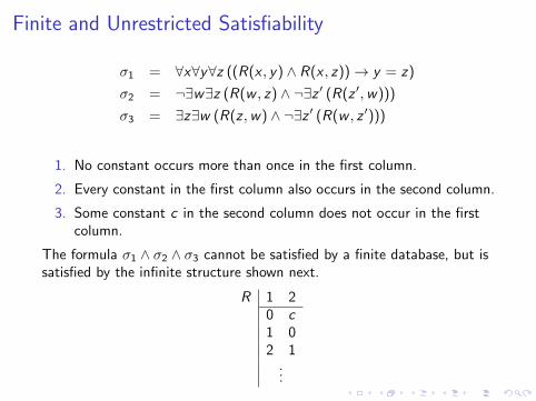
Finite and Unrestricted Satisfiability
σ1 = ∀x∀y∀z ((R(x , y) ∧ R(x , z))→ y = z)
σ2 = ¬∃w∃z (R(w , z) ∧ ¬∃z ′ (R(z ′,w)))
σ3 = ∃z∃w (R(z ,w) ∧ ¬∃z ′ (R(w , z ′)))
1. No constant occurs more than once in the first column.
2. Every constant in the first column also occurs in the second column.
3. Some constant c in the second column does not occur in the firstcolumn.
The formula σ1 ∧ σ2 ∧ σ3 cannot be satisfied by a finite database, but issatisfied by the infinite structure shown next.
R 1 20 c1 02 1
...
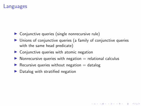
Languages
I Conjunctive queries (single nonrecursive rule)
I Unions of conjunctive queries (a family of conjunctive querieswith the same head predicate)
I Conjunctive queries with atomic negation
I Nonrecursive queries with negation = relational calculus
I Recursive queries without negation = datalog
I Datalog with stratified negation

Outline
Introduction to Datalog with Negation
Reasoning Tasks
Conjunctive Queries
Unions of Conjunctive Queries
Conjunctive Queries with Safe Atomic Negation
Datalog
Datalog with Stratified Negation
Linear Stratified Datalog

Conjunctive Queries
A conjunctive query is an expression of the form
Answer(~x) ← R1(~x1), . . . ,Rn(~xn)
where every variable that occurs in ~x also occurs in some ~xi .
Answer(~x) is called the head, and each Ri (~xi ) is called a subgoal.The set of all subgoals is called the body.
Given a database instance, the answer to this query is defined asfollows:
for every valuation θ,if the facts R1(θ(~x1)), . . . , Rn(θ(~xn)) all belong to thedatabase, then Answer(θ(~x)) belongs to the answer.
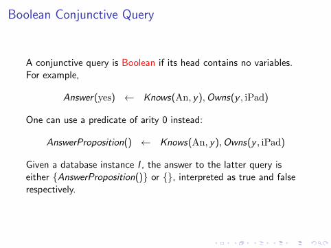
Boolean Conjunctive Query
A conjunctive query is Boolean if its head contains no variables.For example,
Answer(yes) ← Knows(An, y),Owns(y , iPad)
One can use a predicate of arity 0 instead:
AnswerProposition() ← Knows(An, y),Owns(y , iPad)
Given a database instance I , the answer to the latter query iseither {AnswerProposition()} or {}, interpreted as true and falserespectively.

Containment of Conjunctive queries [Ull00]
Let q1 and q2 be conjunctive queries. To test whether q1 v q2:
1. Freeze the body of q1 by turning each of its subgoals intofacts in the database. That is, replace each variable in thebody by a distinct constant, and treat the resulting subgoalsas the only tuples in the database.
2. Apply q2 to this canonical database.
3. If the frozen head of q1 is derived by q2, then q1 v q2.Otherwise, not; in fact, the canonical database is acounterexample to the containment, since surely q1 derives itsown frozen head from this database.
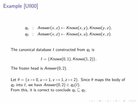
Example [Ull00]
q1 : Answer(x , z)← Knows(x , y),Knows(y , z);
q2 : Answer(x , z)← Knows(x , u),Knows(v , z).
The canonical database I constructed from q1 is
I = {Knows(0, 1),Knows(1, 2)}.
The frozen head is Answer(0, 2).
Let θ = {x 7→ 0, u 7→ 1, v 7→ 1, z 7→ 2}. Since θ maps the body ofq2 into I , we have Answer(0, 2) ∈ q2(I ).From this, it is correct to conclude q1 v q2.

Homomorphism Theorem
Let q1 and q2 be conjunctive queries.A homomorphism from q2 to q1 is a substitution µ such that
I µ maps the head of q2 to the head of q1; and
I µ maps every subgoal of q2 to a subgoal of q1.
For example,
q1 : Answer(x , z)← Knows(x , y),Knows(y , z);
q2 : Answer(x , z)← Knows(x , u),Knows(v , z).
A homomorphism µ from q2 to q1 is µ = {x 7→ x , z 7→ z , u 7→ y ,v 7→ y}.Theorem (Homomorphism Theorem)
q1 v q2 ⇐⇒ there exists a homomorphism from q2 to q1

Valuation and Substitution
I A valuation maps variables to constants.
I A substitution maps variables to variables or constants.
I A renaming is a substitution that is injective (i.e., no twodistinct variables are substituted with the same variable) andmaps no variable to a constant.
I It is understood that any constant is mapped to itself.

Homomorphism Theorem: Example
q1 : Answer(x)← Knows(x , y),Knows(y , x),Knows(y ,Don);
q2 : Answer(v)← Knows(u, v),Knows(v , z).
I A homomorphism µ from q2 to q1 is µ = {v 7→ x , u 7→ y ,z 7→ y}. Hence, q1 v q2.
I There exists no homomorphism from q1 to q2, hence q2 6v q1.

Homomorphism Theorem: Sketch of Proof
Theorem (Homomorphism Theorem)
q1 v q2 ⇐⇒ there exists a homomorphism from q2 to q1
=⇒ Take the canonical database for q1. Since thefrozen head of q1 is in the answer to q1, it must be in theanswer to q2. This implies a homomorphism from q2 to q1
(because the constants in the frozen database mapone-to-one to the variables in q1).
⇐= Let µ be the homomorphism from q2 to q1.Assume that the fact h belongs to the answer toq1 : H ← B on some database I . Then, there exists avaluation θ such that θ(H) = h and θ(B) ⊆ I . Thecomposition θ ◦ µ shows that h ∈ q2(I ).

Rough Visualization of the ⇐= Proof
q2
q1
I
(q2)
(q1)
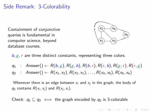
Side Remark: 3-Colorability
Containment of conjunctivequeries is fundamental incomputer science, beyonddatabase courses.
x1nx2n
x3nx4n
x5n���
PPP@@
b, g , r are three distinct constants, representing three colors.
q1 : Answer()← R(b, g),R(g , b),R(b, r),R(r , b),R(g , r),R(r , g)
q2 : Answer()← R(x1, x2),R(x2, x1), . . . ,R(x4, x5),R(x5, x4)
Whenever there is an edge between xi and xj in the graph, the body of
q2 contains R(xi , xj) and R(xj , xi ).
Check: q1 v q2 ⇐⇒ the graph encoded by q2 is 3-colorable

Data Complexity and Query Complexity
For a database I and a query q, what is the time complexity ofcomputing q(I )?
One can distinguish between three complexities:
Data complexity Time complexity in terms of the size of thedatabase, for a fixed query. This is the complexitythat matters in most practical applications.
Query complexity Time complexity in terms of the size of thequery, for a fixed database. E.g., one could fix acanonical database {R(b, g), R(g , b), R(b, r),R(r , b), R(g , r), R(r , g)}.
Combined complexity Time complexity in terms of both the size ofthe database and the size of the query.
The data complexity of datalog is polynomial-time ©, but thequery complexity is already exponential-time for conjunctivequeries (unless P = NP).

Side Remark: Satisfiability
ϕ = (p ∨ q) ∧ (¬q ∨ r) ∧ (¬r ∨ p) ∧ (¬q ∨ ¬r)
q1 : Answer() ← PP(0, 1),PP(1, 0),PP(1, 1),
NP(0, 0),NP(1, 1),NP(0, 1),
NN(0, 1),NN(1, 0),NN(0, 0)
q2 : Answer() ← PP(p, q),NP(q, r),NP(r , p),NN(q, r)
A homomorphism from q2 to q1 is µ = {p 7→ 1, q 7→ 0, r 7→ 0}.µ is also a satisfying truth assignment for ϕ.
Check: q1 v q2 ⇐⇒ the 2-CNF formula encoded by q2 issatisfiable

Query Optimization for Conjunctive Queries
A conjunctive query is minimal if it is not equivalent to anyconjunctive query with a strictly smaller number of subgoals.
TheoremFor every conjunctive query q1 : H ← B1, there exists a subsetB2 ⊆ B1 such that q2 : H ← B2 is minimal and equivalent to q1.
TheoremIf two minimal conjunctive queries are equivalent, then they areidentical up to a renaming of variables.
Outline
Introduction to Datalog with Negation
Reasoning Tasks
Conjunctive Queries
Unions of Conjunctive Queries
Conjunctive Queries with Safe Atomic Negation
Datalog
Datalog with Stratified Negation
Linear Stratified Datalog

Unions of Conjunctive Queries
A union of conjunctive queries is a finite set Q = {q1, . . . , q`} ofconjunctive queries, all with the same head predicate.The semantics is natural: Q(I ) =
⋃`i=1 qi (I ).
TheoremFor Q1 and Q2 unions of conjunctive queries,
Q1 v Q2 ⇐⇒ ∀q ∈ Q1∃p ∈ Q2 : q v p
The proof of ⇐= is straightforward. For the =⇒ direction, seewhat happens if we take the canonical database for any q ∈ Q1.

Query Optimization for Unions of Conjunctive Queries
Check:
Answer(y) ← Knows(y , x),Knows(x , y),Knows(y ,Don)
Answer(y) ← Knows(x , y),Knows(y , x),Knows(y , z)
is equivalent to
Answer(y) ← Knows(x , y),Knows(y , x)

UCQ ≡ SPJRU
σA=c(E ∪ F ) ≡ σA=c(E ) ∪ σA=c(F )
σA=B(E ∪ F ) ≡ σA=B(E ) ∪ σA=B(F )
πX (E ∪ F ) ≡ πX (E ) ∪ πX (F )
ρA 7→B(E ∪ F ) ≡ ρA7→B(E ) ∪ ρA 7→B(F )
E on (F ∪ G ) ≡ (E on F ) ∪ (E on G )
(E ∪ F ) on G ≡ (E on G ) ∪ (F on G )
=⇒ every expression E in SPJRU can be equivalently rewritten inthe form E1 ∪ E2 ∪ · · · ∪ E` where each Ei is union-free (i.e., eachEi is a conjunctive query).
Note: the last two rules result in an exponential blowup in the sizeof the query (but that does not matter if we are only concernedabout data complexity).
Outline
Introduction to Datalog with Negation
Reasoning Tasks
Conjunctive Queries
Unions of Conjunctive Queries
Conjunctive Queries with Safe Atomic Negation
Datalog
Datalog with Stratified Negation
Linear Stratified Datalog
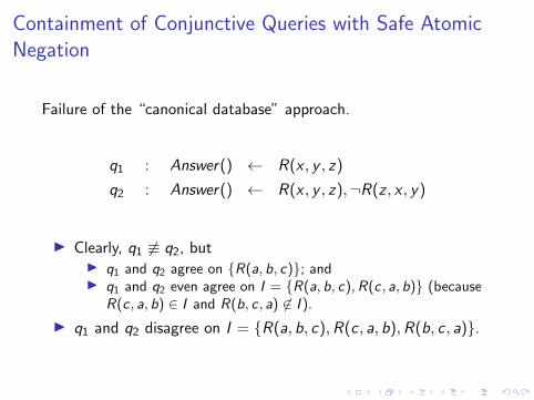
Containment of Conjunctive Queries with Safe AtomicNegation
Failure of the “canonical database” approach.
q1 : Answer() ← R(x , y , z)
q2 : Answer() ← R(x , y , z),¬R(z , x , y)
I Clearly, q1 6≡ q2, butI q1 and q2 agree on {R(a, b, c)}; andI q1 and q2 even agree on I = {R(a, b, c),R(c , a, b)} (because
R(c , a, b) ∈ I and R(b, c , a) 6∈ I ).
I q1 and q2 disagree on I = {R(a, b, c),R(c, a, b),R(b, c , a)}.

Containment of Conjunctive Queries with Safe AtomicNegation
The Levy-Sagiv test [LS93] for testing q1 v q2, where q1, q2 arequeries without constants.
I We use an alphabet A of k constants, where k is the numberof variables in q1.
I We consider all databases I whose active domain is containedin A. If q1(I ) ⊆ q2(I ) for each of these canonical databases,then q1 v q2, and if not, then not.
That is, if q1 6v q2, then there exists a database I whose activedomain contains no more than k constants such thatq1(I ) * q2(I ).
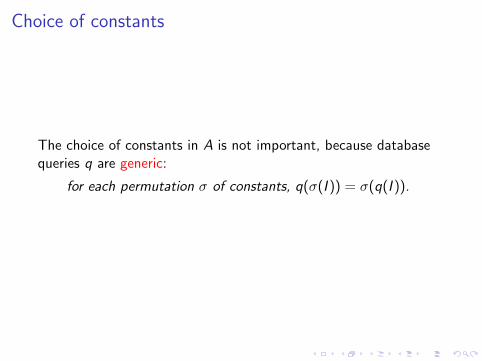
Choice of constants
The choice of constants in A is not important, because databasequeries q are generic:
for each permutation σ of constants, q(σ(I )) = σ(q(I )).

Correctness Proof
1. Assume that for every database I in the Levy-Sagiv test,q1(I ) ⊆ q2(I ).
2. Let E be an arbitrary database, and let t be a fact such thatt ∈ q1(E ). It suffices to show t ∈ q2(E ).
3. Let {c1, . . . , cn} be the (necessarily finite) set of constants thatvariables of q1 are mapped to when showing t ∈ q1(E ).
4. Let D be the database containing all (and only) the facts of E all ofwhose components are in {c1, . . . , cn}. From 1 and genericity, itfollows q1(D) ⊆ q2(D). From t ∈ q1(D) (because t ∈ q1(E )), itfollows t ∈ q2(D).
5. The valuation that shows t ∈ q2(D) maps positive subgoals of q2 tofacts in E , and maps negative subgoals of q2 to facts not in E(Why?). Hence, t ∈ q2(E ). Recall that every variable that occurs inq2, occurs in a nonnegated subgoal of q2 (safety).

Example
q1 : Ans(x , z)← Knows(x , y),Knows(y , z),¬Knows(x , z)
q2 : Ans(x , z)← Knows(x , y),Knows(y , z),Knows(y , u),¬Knows(x , u)
Is q1 v q2?
The query q1 contains three variables. Let A = {0, 1, 2}.I Let I = ∅. Since q1(I ) ⊆ q2(I ) = ∅, this is not a counterexample for
q1 v q2.
I . . .
I Let I = {Knows(0, 1),Knows(1, 0)}, a database whose activedomain is contained in A. We have q1(I ) = {Ans(0, 0), Ans(1, 1)}.Since q1(I ) ⊆ q2(I ), this is not a counterexample for q1 v q2.
I . . .
After a lot (but finite amount) of work, we will have found nocounterexample for q1 v q2. It is correct to conclude q1 v q2.

Example
q1 : Ans(x , z)← Knows(x , y),Knows(y , z),¬Knows(x , z)
q2 : Ans(x , z)← Knows(x , y),Knows(y , z),Knows(y , u),¬Knows(x , u)
Is q2 v q1?
Let I = {Knows(0, 1),Knows(1, 2),Knows(0, 2),Knows(1, 3)}.We have Ans(0, 2) ∈ q2(I ) and Ans(0, 2) 6∈ q1(I ), hence q2 6v q1.
Outline
Introduction to Datalog with Negation
Reasoning Tasks
Conjunctive Queries
Unions of Conjunctive Queries
Conjunctive Queries with Safe Atomic Negation
Datalog
Datalog with Stratified Negation
Linear Stratified Datalog

Datalog Syntax
A set of rules without negation.

Datalog Semantics
Let P be a datalog program.
I We use the term deductive database for a set of facts thatcan use both edb and idb predicates.
I The immediate consequence operator TP maps each deductivedatabase J to the deductive database TP(J) satisfying
1. TP(J) “copies” all edb facts of J;2. TP(J) contains all idb facts that can be derived from J by
executing once every rule of P; and3. no other facts belong to TP(J).
I Given an edb database I , the answer P(I ) is defined as the(unique) smallest (w.r.t. ⊆) deductive database J such thatI ⊆ J and TP(J) = J.
TP is obviously monotone. . .

Immediate Consequence Operator: Example
Let P contain two rules:
A(x , y) ← R(x , y)
A(x , y) ← R(x , z),A(z , y)
LetJ = {R(1, 2),R(2, 3),A(2, 5)}.
Then
TP(J) = {R(1, 2),R(2, 3),A(1, 2),A(2, 3),A(1, 5)};TP(TP(J)) = {R(1, 2),R(2, 3),A(1, 2),A(2, 3),A(1, 3)}.

Multiple Fixpoints
Let P contain one rule:
A(x) ← R(x),A(x)
Let
I = {R(a)};J1 = {R(a)};J2 = {R(a),A(a)}.
Then,
TP(J1) = J1;
TP(J2) = J2.

Undecidability
Theorem
I The containment problem for datalog is undecidable.
I The equivalence problem for datalog is undecidable.
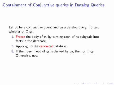
Containment of Conjunctive queries in Datalog Queries
Let q1 be a conjunctive query, and q2 a datalog query. To testwhether q1 v q2:
1. Freeze the body of q1 by turning each of its subgoals intofacts in the database.
2. Apply q2 to the canonical database.
3. If the frozen head of q1 is derived by q2, then q1 v q2.Otherwise, not.
Outline
Introduction to Datalog with Negation
Reasoning Tasks
Conjunctive Queries
Unions of Conjunctive Queries
Conjunctive Queries with Safe Atomic Negation
Datalog
Datalog with Stratified Negation
Linear Stratified Datalog

Syntax of Datalog with Stratified Negation
I a set of safe rules such that
I the program dependence graph (PDG) contains no cycle witha negated edge
Semantics of Datalog with Stratified Negation
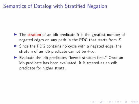
I The stratum of an idb predicate S is the greatest number ofnegated edges on any path in the PDG that starts from S .
I Since the PDG contains no cycle with a negated edge, thestratum of an idb predicate cannot be +∞.
I Evaluate the idb predicates “lowest-stratum-first.” Once anidb predicate has been evaluated, it is treated as an edbpredicate for higher strata.
Recursion and Negation
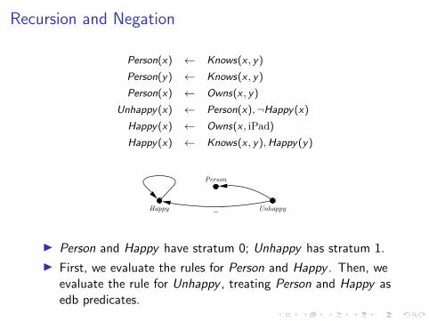
Person(x) ← Knows(x , y)
Person(y) ← Knows(x , y)
Person(x) ← Owns(x , y)
Unhappy(x) ← Person(x),¬Happy(x)Happy(x) ← Owns(x , iPad)
Happy(x) ← Knows(x , y),Happy(y)
−Happy Unhappy
Person
I Person and Happy have stratum 0; Unhappy has stratum 1.
I First, we evaluate the rules for Person and Happy . Then, weevaluate the rule for Unhappy , treating Person and Happy asedb predicates.

The Barber Paradox
There is a male village barber who shaves all and only those menin the village who do not shave themselves.Does the barber shave himself?
Shaves(Barber, x) ← Male(x),¬Shaves(x , x)
The negation in this program is not stratified.
Let I = {Male(Barber)}.
What happens if we try fixpoint semantics?
TP(I ) = {Male(Barber),Shaves(Barber,Barber)}TP(TP(I )) = {Male(Barber)}
There is no fixpoint.
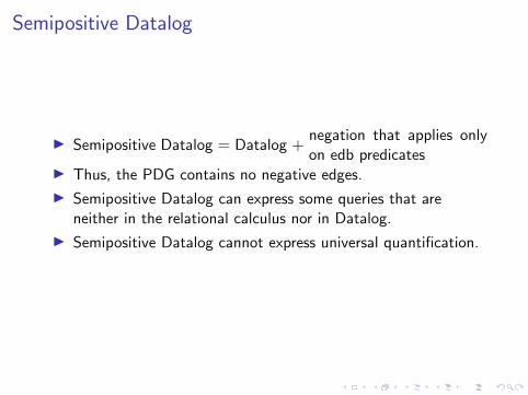
Semipositive Datalog
I Semipositive Datalog = Datalog +negation that applies onlyon edb predicates
I Thus, the PDG contains no negative edges.
I Semipositive Datalog can express some queries that areneither in the relational calculus nor in Datalog.
I Semipositive Datalog cannot express universal quantification.
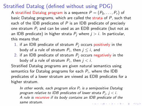
Stratified Datalog (defined without using PDG)A stratified Datalog program is a sequence P = (P0, . . . ,Pr ) ofbasic Datalog programs, which are called the strata of P, such thateach of the IDB predicates of P is an IDB predicate of preciselyone stratum Pi and can be used as an EDB predicate (but not asan IDB predicate) in higher strata Pj where j > i . In particular,this means that
1. if an IDB predicate of stratum Pj occurs positively in thebody of a rule of stratum Pi , then j ≤ i , and
2. if an IDB predicate of stratum Pj occurs negatively in thebody of a rule of stratum Pi , then j < i .
Stratified Datalog programs are given natural semantics usingsemantics for Datalog programs for each Pi , where the IDBpredicates of a lower stratum are viewed as EDB predicates for ahigher stratum.
In other words, each program slice Pi is a semipositive Datalogprogram relative to IDB predicates of lower strata Pj , j < i .A rule is recursive if its body contains an IDB predicate of thesame stratum.

Multiple Stratifications
R(x) ← A(x),¬S(x)S(x) ← B(x)T (x) ← S(x)
The stratification found by the PDG is(P0 :
{S(x) ← B(x)T (x) ← S(x)
,P1 :{
R(x) ← A(x),¬S(x)
).
Another stratification is:(P0 :
{S(x) ← B(x) ,P1 :
{R(x) ← A(x),¬S(x)T (x) ← S(x)
).
It is known that all stratifications are equivalent.
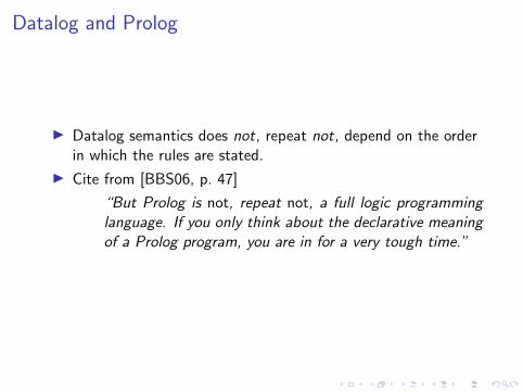
Datalog and Prolog
I Datalog semantics does not, repeat not, depend on the orderin which the rules are stated.
I Cite from [BBS06, p. 47]
“But Prolog is not, repeat not, a full logic programminglanguage. If you only think about the declarative meaningof a Prolog program, you are in for a very tough time.”

Overview
SPJRUD+FP
[Positive] Datalog≡ SPJRU+FP
Stratified Datalog
Linear Datalog≡ SPJRU+TC
Linear Stratified Datalog≡ SPJRUD+TC
UCQ≡ SPJRU
CQ≡ SPJR
Relational Calculus≡ SPJRUD
CQ with Negated Atoms
Semipositive Datalog
without negation
with negation
Outline
Introduction to Datalog with Negation
Reasoning Tasks
Conjunctive Queries
Unions of Conjunctive Queries
Conjunctive Queries with Safe Atomic Negation
Datalog
Datalog with Stratified Negation
Linear Stratified Datalog

Linear Stratified Datalog[Following up on a question by a student in 2017.]A linear program for transitive closure:
Trans(x , y) ← Knows(x , y)
Trans(x , y) ← Knows(x , z),Trans(z , y)
A nonlinear program for transitive closure:
Trans(x , y) ← Knows(x , y)
Trans(x , y) ← Trans(x , z),Trans(z , y)
I Two predicates R and R ′ are mutually recursive if R = R ′ orR and R ′ participate in the same cycle of the dependencegraph.
I A rule with head predicate R is linear if there is at most oneatom in the body of the rule whose predicate is mutuallyrecursive with R.Note: this allows more than one idb predicate in the body.
I A program is linear if each rule in it is linear.

Transitive Closure in SQL
Trans(x , y) ← Knows(x , y)
Trans(x , y) ← Trans(x , z),Knows(z , y)
Ans(y) ← Trans(Jo, y)
Assume that the schema of Knows is [A,B]
WITH RECURSIVE Trans(A’,B’) AS
( (SELECT A as A’, B as B’ FROM Knows)
UNION
(SELECT Trans.A’, Knows.B as B’
FROM Trans, Knows
WHERE Trans.B’ = Knows.A) )
SELECT B’ FROM Trans WHERE A’= "Jo"

Extending Relational Calculus with Transitive Closure
1. Every formula in relational calculus is a formula in TransitiveClosure Logic (TC).
2. If ϕ(x , y , z) is a formula in TC with free variables x , y , z , then
[tclx ,yϕ(x , y , z)](x ′, y ′)
is a formula in TC with free variables x ′, y ′, z .
The semantics is as follows. For any fixed value c for z ,
[tclx ,yϕ(x , y , c)](a, b)
evaluates to true on a database if (a, b) is in the transitive closureof the answer to the query {x , y | ϕ(x , y , c)}.[In general, x , y , z can be sequences of variables.]

In Other Words. . .
[tclx ,yϕ(x , y , z)](x ′, y ′)
is the same as
[fp∆:x ,y ,z (ϕ(x , y , z) ∨ ∃w (ϕ(x ,w , z) ∧∆(w , y , z))](x ′, y ′, z)
See Sections 6 and 7 of “Adding Recursion to SPJRUD”

Example: Graph ConnectivityLet the binary relation E encode the directed edges of a graph, i.e.,E (a, b) holds true if there is a directed edge from a to b.Is the undirected graph associated with E (obtained by ignoringthe directions of the edges) connected?
∀u∀v (ν(u) ∧ ν(v)→ [tclx ,yE (x , y) ∨ E (y , x)](u, v))
where ν(z) is a syntactic shorthand for “z is a vertex”:
ν(z) := ∃w (E (z ,w) ∨ E (w , z))
In linear stratified Datalog:
Adjacent(x , y) ← E(x , y)
Adjacent(x , y) ← E(y , x)
Trans(u, v) ← Adjacent(u, v)
Trans(u, v) ← Adjacent(u,w),Trans(w , v)
V (x) ← Adjacent(x , y)
Disconnected() ← V (u),V (v),¬Trans(u, v)Connected() ← ¬Disconnected()
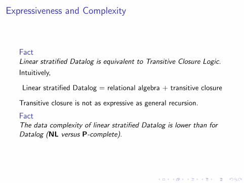
Expressiveness and Complexity
FactLinear stratified Datalog is equivalent to Transitive Closure Logic.
Intuitively,
Linear stratified Datalog = relational algebra + transitive closure
Transitive closure is not as expressive as general recursion.
FactThe data complexity of linear stratified Datalog is lower than forDatalog (NL versus P-complete).

Recursion that is Not Linear
Here is a program that is not linear (and you will not be able tofind an equivalent linear program).
T (x) ← A(x)
T (x) ← R(x , y , z),T (y),T (z)
To give a meaning to this program, think of the variables asplaceholders for Boolean propositions:
I R(p, q, r) says that “p IF (q AND r)”
I A(p) says that “p is TRUE”
So this is an interpreter for [a subset of] propositional logic.

Overview
SPJRUD+FP
[Positive] Datalog≡ SPJRU+FP
Stratified Datalog
Linear Datalog≡ SPJRU+TC
Linear Stratified Datalog≡ SPJRUD+TC
UCQ≡ SPJRU
CQ≡ SPJR
Relational Calculus≡ SPJRUD
CQ with Negated Atoms
Semipositive Datalog
without negation
with negation
Exercise
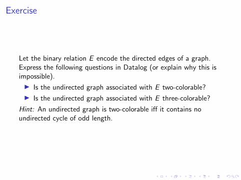
Let the binary relation E encode the directed edges of a graph.Express the following questions in Datalog (or explain why this isimpossible).
I Is the undirected graph associated with E two-colorable?
I Is the undirected graph associated with E three-colorable?
Hint: An undirected graph is two-colorable iff it contains noundirected cycle of odd length.

Exercise
Let the binary relation E encode the directed edges of a graph,without self-loops. Let C be a binary relation such that C (v , c)means that the vertex v has color c . Every vertex has exactly onecolor. Say that a directed path from vertex v1 to vertex v2 iswell-colored if no three successive vertices on the path have thesame color (but two successive vertices can have the same color).Express the following questions in Datalog (or explain why this isimpossible); the disequality predicate 6= can be used.
I Find pairs (v1, v2) of vertices such that there exists nowell-colored directed path from v1 to v2.
I Find pairs (v1, v2) of vertices such that (i) there exists adirected path from v1 to v2 and (ii) all directed paths from v1
to v2 are well-colored.

Executing Datalog Programs in DLV
You can download dlv.exe from http://www.dlvsystem.com/
Three useful commands: dlv -help
dlv input.txt
dlv -filter=Answer input.txt
%%% This is input.txt %%%
%%% The database facts %%%
C(1,blue). C(2,red). C(3,red). C(4,red).
E(1,2). E(2,3). E(3,4). E(4,1).
%%% The Datalog program %%%
V(X) :- E(X,Y).
V(Y) :- E(X,Y).
WCP(X,Y,R) :- E(X,Y), C(X,R).
WCP(X,Y,R) :- WCP(X,Z,S), E(Z,Y), C(Z,R), R != S.
WCP(X,Y,R) :- WCP(X,Z,S), E(Z,Y), C(Z,R), C(Y,T), R != T.
ExistsWCP(X,Y) :- WCP(X,Y,R).
ExistsWCP(X,X) :- V(X).
% Every vertex has a well-colored path to itself...
Answer(X,Y) :- V(X), V(Y), not ExistsWCP(X,Y).
References
Patrick Blackburn, Johan Bos, and Kristina Striegnitz.
Learn Prolog Now!, volume 7 of Texts in Computing.College Publications, 2006.
Alon Y. Levy and Yehoshua Sagiv.
Queries independent of updates.In VLDB, pages 171–181, 1993.
Christos H. Papadimitriou.
Computational complexity.Addison-Wesley, 1994.
Alan M. Turing.
On computable numbers, with an application to the Entscheidungsproblem.Proceedings of the London Mathematical Society, 2(42):230–265, 1936.
Jeffrey D. Ullman.
Information integration using logical views.Theor. Comput. Sci., 239(2):189–210, 2000.