Happy Monday!

Chapter 3.1Exponential Functions

Did we find a non-recursive formula?

You just got a job! You will work 8 hours a day for 4 days. You may choose between three pay rates, BUT you only get a few minutes to make your choice:

Rate Plan A pays $10,000 an hour.

Rate Plan B pays $1,000 your first hour and provides you with a $2,000 an hour raise each subsequent hour. (For instance, you earn $3,000 an hour the second hour, $5,000 the third hour, and so forth.)

Rate Plan C pays one cent the first hour and doubles every subsequent hour. (For instance, you earn two cents an hour the second hour, four cents an hour the third hour, and so forth)

Yay, time to get paid!!!

How much would you make in total for each?

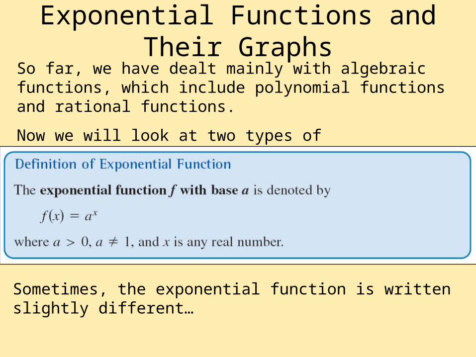
Exponential Functions and Their GraphsSo far, we have dealt mainly with algebraic functions, which include polynomial functions and rational functions.

Now we will look at two types of transcendental functions--------exponential functions and logarithmic functions.

Sometimes, the exponential function is written slightly different…

Investigation Worksheet15-ish minutes.

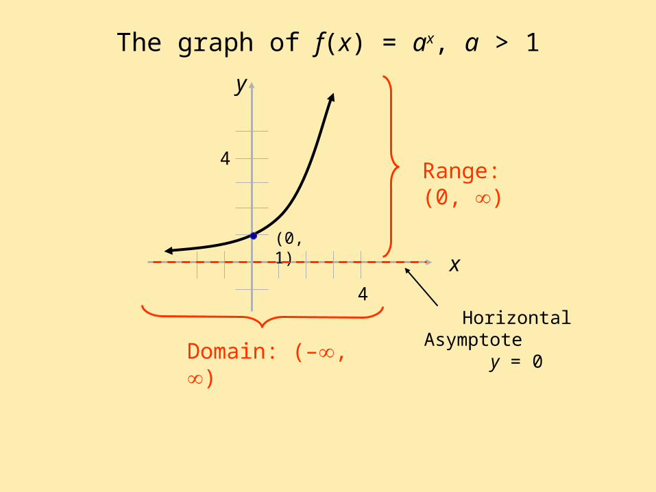
The graph of f(x) = ax, a > 1

y

x(0, 1)

Domain: (–, )

Range: (0, )

Horizontal Asymptote y = 0

4

4

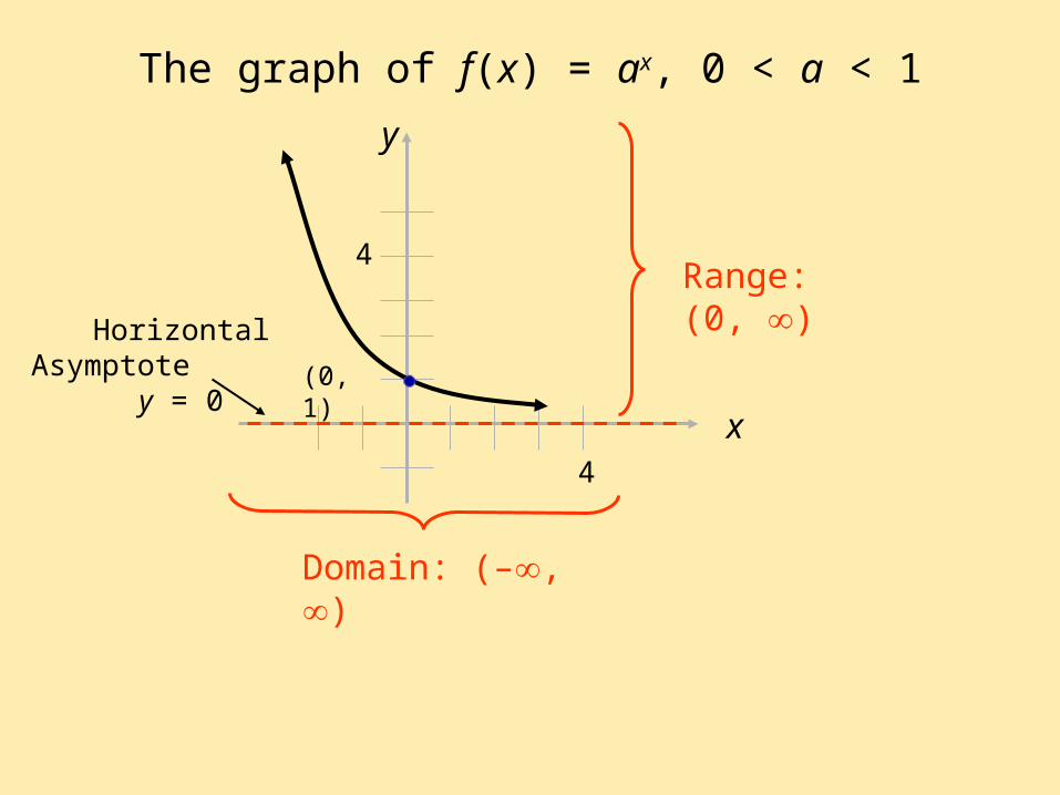
The graph of f(x) = ax, 0 < a < 1

y

x

(0, 1)

Domain: (–, )

Range: (0, )

Horizontal Asymptote y = 0

4

4

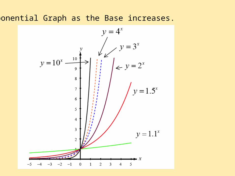
Exponential Graph as the Base increases.

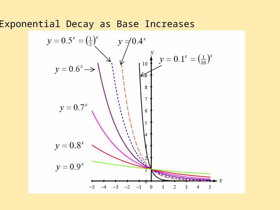
Exponential Decay as Base Increases

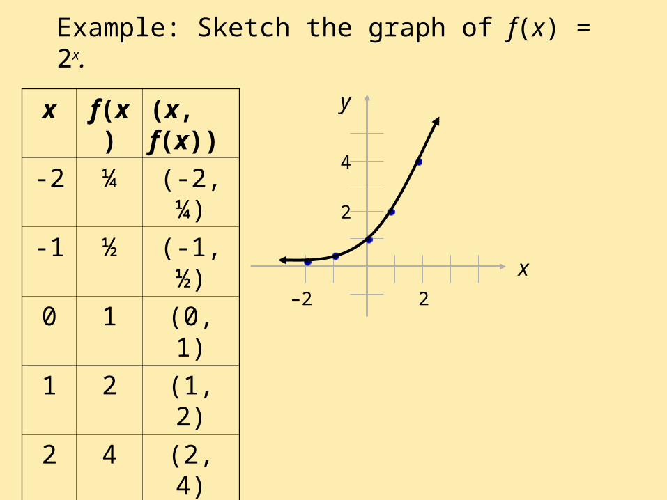
Example: Sketch the graph of f(x) = 2x.

x

x f(x) (x, f(x))

-2 ¼ (-2, ¼)

-1 ½ (-1, ½)

0 1 (0, 1)

1 2 (1, 2)

2 4 (2, 4)

y

2–2

2

4

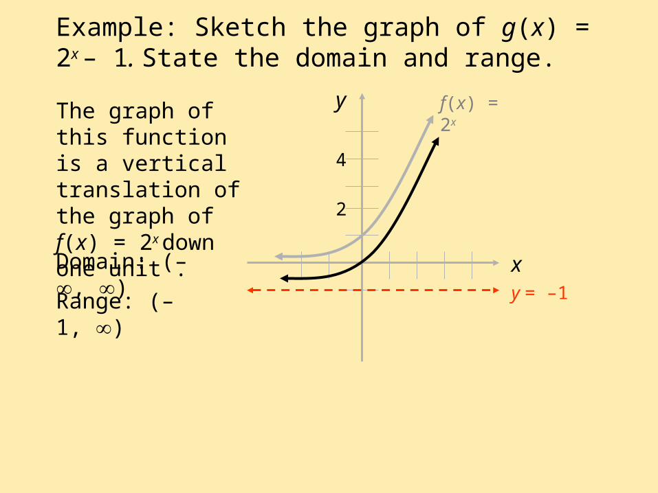
Example: Sketch the graph of g(x) = 2x – 1. State the domain and range.

x

yThe graph of this function is a vertical translation of the graph of f(x) = 2x

down one unit .

f(x) = 2x

y = –1 Domain: (–, )

Range: (–1, )

2

4

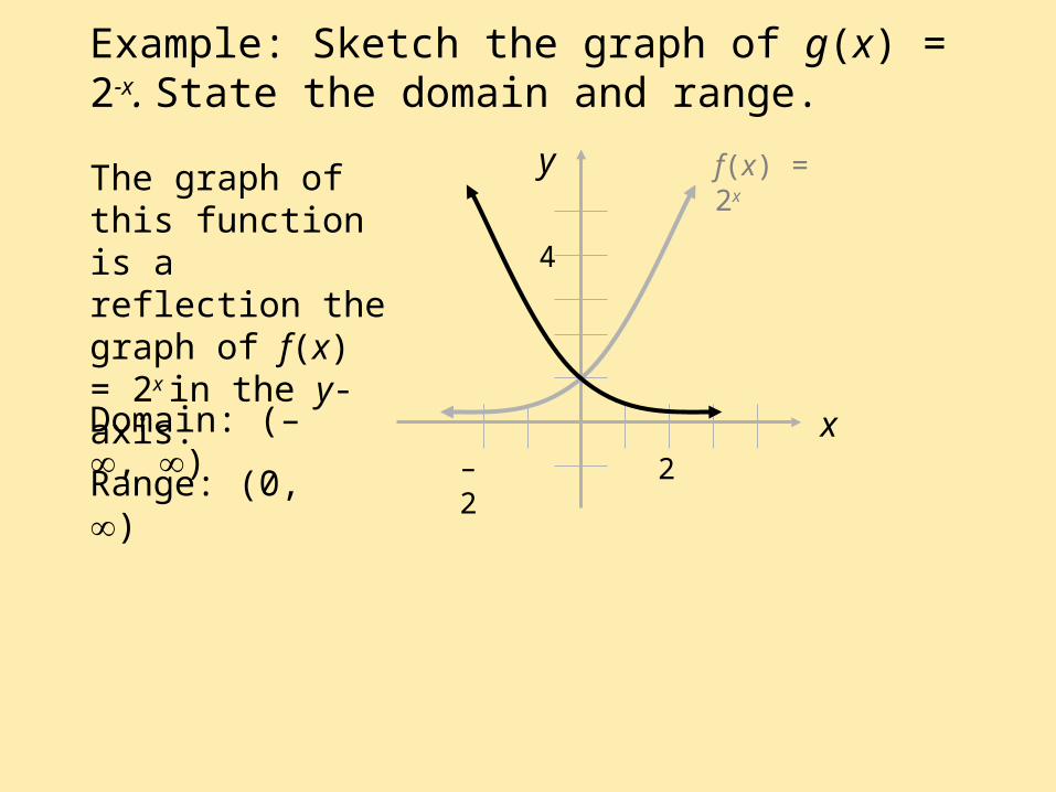
Example: Sketch the graph of g(x) = 2-x. State the domain and range.

x

yThe graph of this function is a reflection the graph of f(x) = 2x in the y-axis.

f(x) = 2x

Domain: (–, )

Range: (0, ) 2–2

4

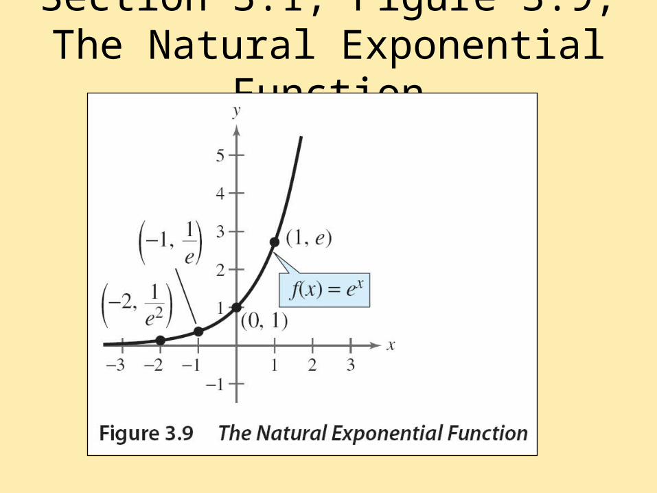
Section 3.1, Figure 3.9,The Natural Exponential Function

Graphing Shifts

You can shift the axis or you can shift the anchor points.

If it’s in the air with the exponent, it affects the graph horizontally.

If it’s down on ground level, it affects the graph vertically.

Remember shifts inside parentheses go in reverse.

Negatives are a reflection.

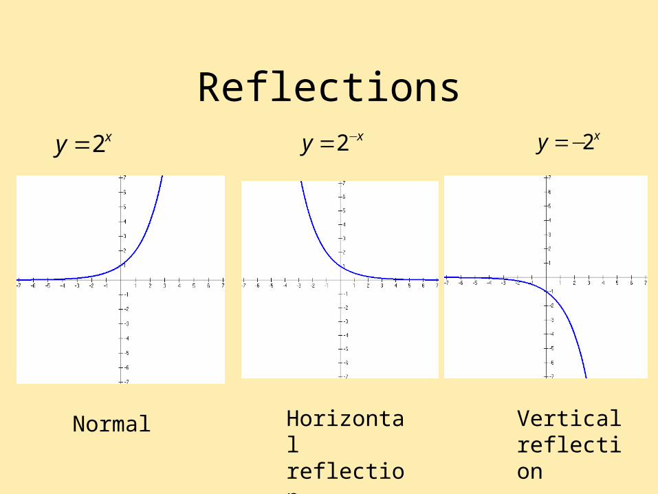
Reflections2xy = 2 xy −= 2xy =−

Normal Horizontal reflection

Vertical reflection

Shiftsmoving points

In the exponent is sideways, backwards.

Ground level is vertical, just like it says.

12

2

4x

xy

y +=

=

−

The key points will move left 1 and down 4

What makes an exponential function different from a

quadratic function (or any power?)

Let’s look at some data!

Functions Are Fun!

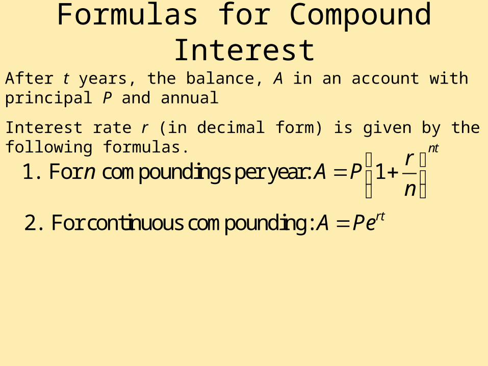
Formulas for Compound Interest

After t years, the balance, A in an account with principal P and annual

Interest rate r (in decimal form) is given by the following formulas.

1. For compoundings per year: 1

2. For continuous compounding:

nt

rt

rn A P

n

A Pe

⎛ ⎞= +⎜ ⎟⎝ ⎠

=

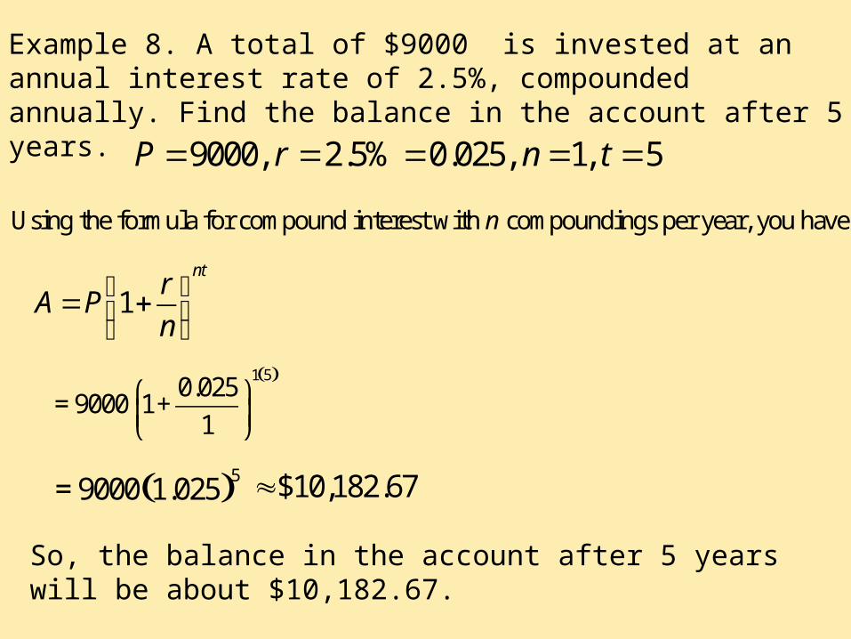
Example 8. A total of $9000 is invested at an annual interest rate of 2.5%, compounded annually. Find the balance in the account after 5 years.

9000, 2.5% 0.025, 1, 5P r n t= = = = =

1nt

rA P

n⎛ ⎞= +⎜ ⎟⎝ ⎠

( )1 50.025

9000 11

⎛ ⎞= +⎜ ⎟⎝ ⎠

( )59000 1.025= $10,182.67≈

So, the balance in the account after 5 years will be about $10,182.67.

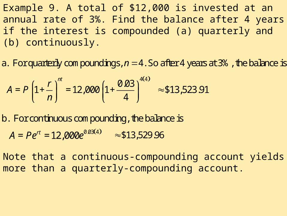
Example 9. A total of $12,000 is invested at an annual rate of 3%. Find the balance after 4 years if the interest is compounded (a) quarterly and (b) continuously.

a. For quarterly compoundings, 4. So after 4 years at 3%, the balance isn =

( )4 40.03

1 12,000 14

ntr

A Pn

⎛ ⎞ ⎛ ⎞= + = +⎜ ⎟ ⎜ ⎟⎝ ⎠ ⎝ ⎠

$13,523.91≈

b. For continuous compounding, the balance is( )0.03 412,000rtA Pe e= = $13,529.96≈

Note that a continuous-compounding account yields more than a quarterly-compounding account.

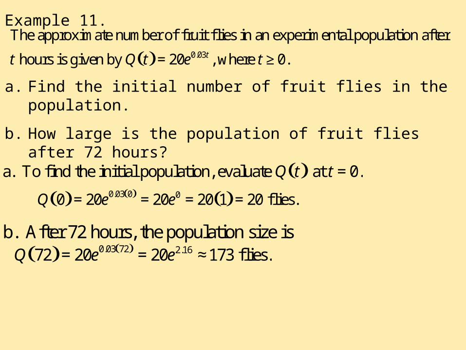
Example 11.

( ) 0.03

The approximate number of fruit flies in an experimental population after

hours is given by 20 , where 0.tt Q t e t= ≥

a. Find the initial number of fruit flies in the population.

b. How large is the population of fruit flies after 72 hours?

( )a. To find the initial population, evaluate at 0.Q t t =

( ) ( ) ( )0.03 0 00 20 20 20 1 20 flies.Q e e= = = =

b. After 72 hours, the population size is( ) ( )0.03 72 2.1672 20 20 173 flies.Q e e= = ≈

Classwork!

Page 185#’s 7-21 odd 51-61 odd