hardware-friendly genetic regulatory networks · mimics the properties of poetic cells, the basic...

Hardware-Friendly Genetic Regulatory Networks

in POEtic tissue

Arne Koopman

Intelligent Systems Group, Institute for Information and Computing Sciences, Utrecht University Correspondence e-mail address: [email protected]

Submitted in partial fulfilment of the requirements for the degree of Master of Science Student

Adrianus Cornelis Matheus Koopman Period

August 2003 - February 2004 Supervisors Intelligent Systems Group, Utrecht University, the Netherlands

Prof. Dr. John-Jules Ch. Meyer Dr. Marco A. Wiering

Autonomous Systems Laboratory, Swiss Federal Institute of Technology in Lausanne, Switzerland

M.Sc. Daniel Roggen

Acknowledgements

This research project is the result of a fruitful collaboration between the Adaptive Intelligence Laboratory at Utrecht University and the Autonomous Systems Laboratory at the Ecole Polytechnique Fédérale de Lausanne. Its success has depended much upon the input of a great many individuals whom I would like to sincerely thank.

First and foremost, I would like to extend much gratitude to Dario Floreano and Daniel Roggen for inspiring me with discussions stemming from our shared view of bio-inspired systems combined with a pleasant three month stay in their laboratory.

Closer to home, the insight of John-Jules Meyer and Marco Wiering was invaluable in helping me to co-found the Adaptive Intelligence Laboratory, which lead to several successful projects including fruity bots and evolutionary robotics.

This experience would not have been the same without the company of two fellow students: Matthijs van Leeuwen and Jilles Vreeken. In addition to the many laughs, making the lab a wonderful place to spend time and the sharing of ideas have inspired the development of many exciting projects that would not have otherwise happened.

Having said this, I still have many more people to thank: family and friends for engaging tirelessly into conversations about this subject, and a small list of people deserve a note here for their inspiration, sharing of ideas, reviewing or otherwise helpful comments: Mototaka Suzuki, Jesper Blynel, Claudio Mattiussi, Kathryn Potter, Josh Bongard and Tom Quick.

Finally I would like to thank the foundations that made my visit to the EPFL and the last months of my studies financially possible; Fundatie van de Vrijvrouwe van Renswoude, Dr Hendrik Muller's Vaderlansch Fonds and the Schuurman Schimmel - van Outeren Stichting.

4

Table of Contents Acknowledgements 3 Table of Contents 4 Chapter 1 - Introduction 6

1.1 Thesis outline 7

Chapter 2 – Biological Development 9 2.1 Biological development 9 2.2 Phylogeny 9 2.3 Ontogeny 11 2.4 Epigeny 13 2.5 Summary 13

Chapter 3 – Evolvable Hardware 14

3.1 Introduction 14 3.2 Evolutionary computation 15 3.2.1 Genetic algorithms 15 3.2.2 Genetic programming 17 3.2.3 Evolution strategies 17 3.3 Evolvable hardware principles 18 3.4 Evolved hardware 19 3.5 Summary 21

Chapter 4 – Artificial Ontogeny 23

4.1 Ontogenetic techniques 23 4.2 L-Systems 24 4.3 Reaction-Diffusion Systems 25 4.4 Bio-Chemical Networks 25 4.5 Random Boolean Networks 26 4.6 Genetic Regulatory Networks 27 4.6.1 GRN research 27 4.7 Summary 29

Chapter 5 – POEtic tissue 31

5.1 POEtic architecture 31 5.1.1 Phylogeny 31 5.1.2 Ontogeny 32 5.1.3 Epigeny 32 5.2 POEtic hardware 33 5.2.1 Organic subsystem 33 5.2.1.1 POEtic molecules 33 5.2.1.2 Routing layer 34 5.3 POEtic design 34 5.4 POEtic research 34

Chapter 6 – POEtic GRN Cells 36 6.1 GRN cell behaviour 36 6.1.1 Regulation 37 6.1.1.1 Minimal level encoding 38 6.1.1.2 MinMax level encoding 38 6.1.2 Decay 39 6.1.3 Diffusion 39 6.2 Simulated GRN cells 39 6.3 Hardware implementation 40 6.3.1 Decay pathway 41 6.3.2 Regulation pathway 41 6.3.3 Diffusion pathway 41

Chapter 7 - Experiments 42

7.1 Auto response 43 7.2 Patch growth 43 7.2.1 Basic growth 44 7.2.2 Scalability 45 7.2.3 Gene length 46 7.2.4 Behavioural analysis 47 7.3 Fault tolerance 48 7.3.1 Flush cells 49 7.3.2 Freeze genome decoding 49 7.3.3 Kill cells 50 7.3.4 Insert void cells 51 7.3.5 Behavioural analysis 51 7.4 Oscillation 53 7.4.1 Single cell oscillation 53 7.4.2 Multiple cell oscillation 54 7.4.3 Behavioural analysis 55 7.5 Robotic control 56 7.6 Conclusion 57

Chapter 8 - Conclusions 58

Appendix A – Hardware Details 60

A.1 Global overview 60 A.2 Functional decomposition 61 A.2.1 Regulation module 61 A.2.2 Decay module 62 A.2.3 Diffusion module 63 A.3 Building blocks 64 A.3.4 Serial 1bit adder 64 A.3.5 Serial 1bit subtractor 64 A.3.6 Serial Multiplier 65 A.3.7 Serial Switch Comparator 66 A.3.8 Serial Divider 67 A.3.9 Selectable Memory Cell 67

Appendix B – Software Details 68

B.1 Design 68 B.2 Implementation 69 B.3 Future work 69

Appendix C - Glossary 70 Bibliography 72

1 Introduction

6

Chapter 1

Introduction

The breakdown of important machinery is unreasonably irritating. Regrettably current electronic devices are brittle with respect to their operation requirements; they produce unwanted results or completely stop due to noise or other unexpected environmental conditions. Until now the creation of fault tolerant electronic devices, machines that can somehow cope with less perfect unpredictable conditions have been an unresolved topic. On the contrary, an enormous tolerance for injuries is seen in biological organisms, to the extent that some organisms even manage to grow new limbs. Therefore, we believe that incorporating bio-inspired techniques into electronics may improve the fault tolerance of electronic circuits, allowing systems to sustain heavier environmental stress or to maintain reasonable performance until it is replaced.

In the last few decades interest in mimicking biological systems has grown to the point that this has inspired an entire new research branch as part of the Artificial Intelligence field. Biology, and more specifically evolution, has inspired a technique called Evolvable Hardware, which leads to interesting results in electronic circuit design. However it is fundamentally hard using this method to produce large and complex circuits. One way to solve this is by growing larger circuits from smaller material. Artificial Ontogeny is a research field that targets the growth of structures and includes a wide variety of approaches. This thesis presents a hardware friendly approach inspired by both fields that produces growing circuits based upon a bio-inspired architecture. More specifically, the inspiration from genetic regulatory networks provides a means to include some degree of fault tolerance in these grown structures.

The Future and Emerging Technologies programme (IST-FET) spans many research projects funded by the European Community. One of these projects, the POEtic project, aims at the development of a hardware bio-inspired architecture; an evolvable, self-repairable, learning and growing hardware chip called POEtic tissue. For this three year project a team of researchers already active within the field joined to form the POEtic team; the Swiss Federal Institute of Technology in Lausanne (EPFL), the University of York, the Technical University of Catalunya (UPC), the University of Glasgow, and the University of Lausanne (UNIL). One aim of the project is to try and tackle challenging problems in the field of evolvable hardware, such as fault tolerance.

1.1 Thesis outline POEtic tissue, has nothing to do with “Roses are red, Violets are blue …”. Its name is derived from three distinguished ways of development in organisms: Phylogeny (evolution), Ontogeny (growth) and Epigeny (learning) [32]. The thesis will start with an outline of the biological source of inspiration for this work. Phylogeny is associated with evolution, which is the adaptation of a species to environmental conditions. Evolution has inspired a part of computer science in the form of evolutionary algorithms. These search algorithms use operators like mutation, crossover, and selection and mimic their biological counterparts. By representing problem parameters in a string of symbols, called an artificial genome, this method can search for adequate solutions. Ontogeny is related to the growth of an individual, either by cellular division or differentiation. This process is modelled in computer science on various levels of abstraction, from plant development to the regulation of genes. Ontogeny plays an important role in ‘building’ an individual from its ‘building plan’. The biological genome is too short to completely determine all characteristics in an organism. Growth based upon the genetic material is biology’s way to efficiently use the genetic material and to produce all symmetrical and modular structures seen in nature. Individuals are constantly interacting with the environment and learn from experience, a phenomenon referred to as epigeny. Artificial neural networks are well-known computer applications related to epigeny. These networks contain nodes that mimic biological neurons and use experience to adapt the network connections. All these biological forms of adaptation thus operate on different time-scales, from the adaptation of a species, via the adaptation to environmental influences during the whole life of an individual, to the quick adaptation to daily experiences.

All of these forms of adaptation have influenced a wide range of areas, like the automatic creation of electronic circuits. Evolvable Hardware is a research field which focuses on using evolution to create electronic circuits. An electronic circuit can be described by several parameters: the type of used components, the properties of the components, and their interconnection. By representing these parameters in an artificial genome the evolutionary algorithm can search for suitable circuits. This search is directed by a performance measure that represents the optimal behaviour of the circuit. The current state of this research field is described in chapter 3.

We will see that in order to increase the complexity of evolved hardware, some features to the original concept may have to be added. One of these is the growth of structures and several of such approaches are present in the research field Artificial Ontogeny. We present the various approaches in the field to determine which would be suitable for aiding evolvable hardware. From these we will focus on genetic regulatory networks, which are an abstraction of the biological process in which genes regulate the expression of other genes. This process is involved in nature to produce cell differentiation and thus may be useful to grow structures.

The link presented in this work between these two computer science approaches, artificial evolution and artificial ontogeny, comes together in POEtic tissue. We will discuss the POEtic architecture which reflects the three different biological developmental models. The POEtic tissue is based upon this architecture, a hardware chip that allows the implementation of adaptive techniques in hardware.

2 Biological Development

8

In absence of the final POEtic tissue, we first created a simulator that mimics the properties of POEtic cells, the basic building blocks of POEtic tissue. Using this simulator we performed various initial experiments to gain insight in the minimal requirements needed to obtain basic gene regulation behaviour. Based on this experience we were able to design a POEtic cell that combines evolution with growth. These simulated cells were placed in a grid to form a POEtic tissue of these ‘GRN cells’, and were used to test their abilities on several tasks. One of these set of experiments is related to the issue of fault tolerance. As a GRN operates on a dynamic concentration of artificial proteins, this could make it well suited for compensating injuries. These proteins are represented by type specific concentrations stored in a table of the cell. Cells are damaged in various ways and are tested for their robustness to the injured faults when growing a patch of cells. Since proteins play an important role in genetic regulation, the temporary removal of proteins is one kind of possible injury. Moreover we tested the performance of the cells when either disabling the regulation mechanism or completely killing a cell.

Although the POEtic chip itself does not exist at the time of this writing, it is possible to create a description of a POEtic cell that can be eventually downloaded onto the chip. One particular software implementation is translated in the basic hardware elements of POEtic tissue. A full description of the developed hardware ‘POEtic GRN cell’ is presented in one of the appendices. These hardware cells can be used in future work to generate experimental data from the POEtic tissue chip.

Chapter 2

Biological Development 2

POEtic tissue is a biologically inspired electronics architecture form based upon established developmental methods that are common for all known life forms [60]. As biological organisms present creative, robust and efficient solutions to adapt to fluctuating environmental factors, mimicking natural development promises benefits for electronics.

Biological developments operate on various timescales, from long-lasting adaptation of a species to memorizing short-term events. While each type is placed on a separate axis, the optimal performance in terms of adaptively relies on their interaction. As most bio-inspired research until now is restricted to one developmental axis, an electronic chip able to combine types of development may provide a suitable substrate for systems that incorporate these synergetic effects as seen in nature.

2.1 Biological development Until the 18th century it was commonly assumed that the growth of organisms only involved the increase in size of preformed structures in the embryo. The cell theory proposed by Schleiden [78] was a breakthrough with regard to body structure formation. Organism development is based on a string of inheritable information, the genome. Despite its seemingly large size the genome is much too small to describe all details of the adult directly. Adult humans for example, consist of 60 trillion cells; the genome however contains ‘only’ 2 billion encoding alleles. Moreover, not all genes in the genome are expressed or used in the organism’s development. A large proportion of the genome contains repetitive blocks and is non-expressive; only 2 percent [38] forms coding material and is transcribed into useful proteins.

Development of an organism and environmental adaptation takes place at various levels, each on different axis. This complete process can be attributed to three distinct processes: phylogeny, ontogeny and epigeny. Evolution of a species is placed on the phylogenetic axis, which constantly rearranges the genetic material from one generation to another to suite the changing demands over a long period of time. Starting at conception, genetic material is used to form and repair structures within the individual. These kinds of developmental processes are grouped together on the ontogenetic axis. During the lifetime of an individual, it constantly learns from the interaction with its environment, such as seen in the adaptive nervous- and immune system, which is referred to as epigeny [55]. The combination of these processes is present in most life forms we see in nature and gives rise to their huge resilience.

2.2 Phylogeny The exact origin of the genetic material still remains a point of debate [11]. However, basic properties of this material were uncovered in the previous century. Inheritable traits reside in the genome of an organism: a haploid or diploid chain of nucleotides [1]. Each nucleotide can attach one out of four


10

bases: adenine, cytosine, guanine or thymine; hence that the length of such a string is measured in base pairs. This way of encoding information is universal to all known species. A gene was originally thought to be simply a sequence of nucleotides expressed as a specific characteristic in an individual. However, recent studies have shown that gene function is much more complex, extending far beyond early definitions [1].

This information encoded in the genome may not be readily accessible, as DNA normally is folded compactly to minimize environmental damage. This packaging is partially induced by specific type of proteins called histones that spontaneously wrap it into a compact organization [1]. Histone DNA complexes, also called nucleosomes, are further packed into loops and are held together by a scaffold. In order to decode a single gene these multiple levels structure must be unravelled, resulting in a ten thousand-fold expansion of the DNA (see fig. 1).

Despite the resistance of compact DNA to environmental damage, mutation is still possible. Mutation results from external influences such as radiation or from errors in DNA replication. Errors of the latter type include deletion, duplication, inversion, insertion, transposition, translocation and point mutation of the genetic material. While the probability of mutation should be the same for any base pair or sequence in a DNA strand, the rate of mutation seems to be dependent upon the environment; stress due to harsh conditions may result in a higher mutation rate [41]. Although the results of such mutations tend to be null or negative, positive mutations that improve the likelihood of survival for an individual are possible.

Not all information in the genome is used to describe characteristics of the individual. Over fifty percent of the genome tends to be non-coding repetitive DNA to which no purpose seems to have been assigned. In the remaining part of the genome, a distinction is made between non-expressed genes, or exons, and genes that cause a phenotypic change, or introns. The genomes of more evolved organisms contain more exons than lower organisms like bacteria [6]. This can be explained by the fact that reproduction speed is beneficial for the survival of the latter range of species, which directly relates to a shorter exon-poor genome with only essential nucleotides to be copied. This highly space efficient genome contrast to the more modular organised DNA found in higher organisms.

Genetic material of both parents is combined into one single genome by a process called crossover or recombination, which transfers characteristics of

Figure 1. The chromosome is unfolded through an intricate process involving histone blocks. After this whole process is completed, which also involves the recruitment of transcription factors (see text), the naked DNA can be transcribed [1].


both parents into the offspring. A creature has to be able to cope with environmentally harsh conditions and natural selection may drive the genetic material to successfully adjust itself over time. Fitter individuals have a higher chance of reproduction and therefore generate more offspring, which in effect may lead to the persistence of its genetic properties within the population. So on a long time scale, the population has a certain probability to contain increasingly better adapted individuals.

2.3 Ontogeny Adult organisms originate from a single cell, the zygote, which is created through the merging of an egg with a sperm cell. The zygote is the origin of all other cells in the body, and is able to create the complete individual from the information contained in the genome. Rapid division of the initial zygotic stem cells and extensive cell differentiation is critical to creating a complex individual from the single progenitor cell. Cellular division, while continuously duplicating the genome for each cell, produces all the cells in an organism’s body. However the contained genetic information is not expressed identically in each cell. The location in the organism’s body determines its function, a process that is called cellular differentiation.

At the start of the embryonic development, phase gradients of chemicals called morphogens appear and break the symmetry in the grown bulk of cells [7]. These gradients form the foundation on which more complex structures may be grown with use of a process called gene regulation. This leads to intricate biochemical networks that produce expressed traits in the organism.

A cell type is mainly determined by the concentrations of key proteins within a cell [78]. Proteins are composed of chains of amino acid strings, and different proteins have different roles, ranging from catalytic enzymes to structural wound healing proteins. The exhibited protein function is based on its one-dimensional sequence and on secondary, tertiary and quaternary structure. Although the sequence remains constant and initially determines the folding of the string, protein structure may change over time as part of its functionality. Intercellular protein-protein interactions produce intricate biochemical networks that further increase the complexity of the information flow. Proteins interact when their three-dimensional structures are complementary.

According to the central dogma of molecular genetics information flows only unidirectionally from genotype to phenotype and as part of that a DNA sequence is translated via RNA into proteins. Recent findings like, RNA viruses

Figure 2. A regulatory gene produces a repressor protein that binds to another location, a promoter or cis region, on the genome and in effect represses the transcription of the subsequent genes and their related expression [78].


12

(RNA to DNA), prions (protein misfolding), reverse transcription (RNA to DNA) and self-replicating RNA are numerous counterexamples that challenge the concept of one directional flow of information [41]. The general pathway starts with transcription of DNA residing in the cell nucleus into messenger RNA (mRNA) via a process that removes all exons. This mRNA travels outside of the nucleus and is transcribed into proteins. These proteins play a role in the intra- and inter-cellular communication, and can travel from the interior of one cell via plasma membrane receptors to a neighbouring cell interior.

Another interesting role for proteins is their part in the regulation of the expression of genetic material. This gene expression happens simultaneously at multiple locations on the genome of a cell. The rate at which transcription occurs varies per location due to factors like: DNA methylation and current conformation, external stimuli and the presence of transcription factors [15]. In order to express a gene a general transcription factor (GTF) selects the suitable part of the genome that has to be unfolded to a “naked” state (see fig. 1). Specific remodelling machines are recruited by the GTF and make the nucleosomes ready for transcription by loosening the histones through acylation [43]. In effect, transcription factors determine whether or not a nearby gene is expressed. So if we consider a gene, it has some associated regions called either promoters or enhancers (see fig. 2); the former are usually nearby in the sequence, the latter may be widespread in the genome and are moved nearby in three-dimensional space by folding the strand of genetic material between them.

A transcription factor is built up from a collection of proteins that have to be recruited for it to be functional. Several specific transcription factors are found in nature and can bind to specific genetic sequences. When recruitment is complete, the GTF begins to read and transcribes the gene into RNA. So each of these binding regions can be considered as ‘locks’, that are only opened when all necessary proteins, or ‘keys’ are recruited. Since DNA transcription produces proteins, the gene product itself can be recruited by another GTF and thus play a role in the regulation of other genes [1]. This leads to genetic regulatory networks in which genes regulate and are regulated by other genes. There are two main regulation-transcription relations (see fig. 3). In expression, normally “silent” genes are activated when a certain combination of proteins are present. In inhibition, a repressor protein can block an otherwise active transcription. Through gene regulation the static information contained in the genome is translated into a dynamic protein representation, the proteome and has

Figure 3. Either the binding of a protein complex starts transcription or blocks it, switching the gene on or off respectively [1].


influence on the cellular differentiation. Each cell contains a similar genome, but has different proteomes expressed from it due to its location in the body and thereof resulting protein concentrations.

2.4 Epigeny Adaptation to the environment during an organism’s lifetime is referred to as epigeny and is seen in the nervous- and immune system [78]. The nervous system forms an intricate network of connections, or synapses, each of them with several connectivity properties. The encoding capacity of the available 4*104 genes is much too short to describe the approximately 1014 synapses in the human brain. Environmental interaction constantly reshapes the connectivity and neural properties of the nervous system using experience feedback. Growth and activity of biological neurons is partly induced by chemical substances surrounding the neural cell; when dendrites and axons grow their growth cones are guided by chemical substances. In the last century much research has been done with regards to the operation of biological neurons in the field of neuroscience, but much is still unclear. A detailed introduction into the field of neural networks is beyond the scope of this work and cropping it down would be a shame to the interested reader, since excellent introduction material is currently available [20].

2.5 Summary Biology’s development can be categorised in three different axes and have found their ways in computer science. Phylogeny has inspired a class of search algorithms, Evolutionary Algorithms, which use an artificial genome to represent search parameters. Growth of structures is approached via a wide variety of methods and can be grouped in a field called Artificial Ontogeny. Although not all Machine Learning methods reflect bio-inspired epigenetic characteristic, they all incorporate learned experience during an individual’s life-time. We will focus on the first two axis; evolvable hardware and evolutionary algorithms followed by Artificial Ontogeny in its various forms as both axis are implemented in our model.


14

Chapter 3

Evolvable Hardware 3

Electronic circuit design has always been a specialized engineering profession, and is sometimes regarded as an art, especially in the case of analogue circuit design [27]. Normally engineers use specific heuristics to guide their design process, which take into account properties like tolerance and ease of design. Although this creation process has proven to work in conventional applications, abandoning it can give robustness and creativity needed outside this application domain. Examples of such domains are highly fault tolerant circuits and circuits for which the operating conditions are not fully specified; e.g. robot controllers. Improvements in this area may arise from the use of artificial evolution for automatic circuit design, which is termed evolvable hardware (EHW) [24].

3.1 Introduction In the electronic circuit design process, an engineer relies on heuristics and the reuse of existing building blocks. Although this relieves the designer of reinventing everything from scratch, it does steer the process that produces the eventual solution in a certain direction. Because electronics have to operate in various unpredictable conditions, hands-on experience shaped these heuristics to reduce external influences like crosstalk, temperature dependence and signal noise. As electronics tend to miniaturize, these influences will become a difficult problem for engineers to tackle. The art of designing relies on the use of precise a-priori models that describe subcomponent properties. In general, automatic design does not have to rely on fully described subcomponents, and may concurrently find exploits unseen by human designers, who draw inspiration only from a building-block bound solution space. For example, the amplification of a bipolar transistor, β, varies widely between each item even within the same specific manufacturing batch due to its production process; conventional design uses a minimal value all produced items obey, in contrast to automated design which could exploit the actual value to produce more efficient circuits.

An effective approach for automatic electronic circuit design must reflect demands such as the ability to handle incomplete descriptions, uncertainty and noise, independent of a-priori schemes, creativity and of course it must be applicable to our particular field of interest: electronic circuit design. Fortunately, biology has presented us with that most creative design principle: evolution. Using evolutionary algorithms as an automated design method, evolvable hardware (EHW), may have several benefits. In addition to the exploitation of physical characteristics, EHW may also lead to unconventional or more efficient designs. Moreover as EHW is able to adjust to environmental conditions, hardware constantly adapts in order to meet its requirements.

3.2 Evolutionary computation Over the last decades, various forms of evolution inspired algorithms have been used for a wide range of applications. None of these have been intended to exactly model the natural evolutionary process. It seems that using some of its known key principles already lead to practical algorithms. All basic algorithms use an artificial genome, which is commonly implemented by a string of bits or characters from a given alphabet. The parameters of a candidate solution are encoded in a string, which may be seen as genetic material. In the case of circuit design, it would represent a certain configuration of the circuit.

3.2.1 Genetic algorithms Maybe the most famous work in this field comes from John Holland [25], who presented a direct abstraction from biological evolution and stores properties in a string. As the parameters within the string are composed of characters of an abstract alphabet, the operating genetic algorithm is task independent and can be reused. While genetic algorithms (GA) have been combined with other search algorithms, hybrid GAs, the basic algorithms merely use mutation and crossover operators to search for optimal solutions occurring in various forms (see mathbox genetic algorithm).

Each possible solution is encoded in a genetic string, the genotype, which code the parameters to be optimized. The functionality of the system related to this set of parameters is called an individual or the phenotype. Genotype elements determine the characteristics of the phenotype and are mapped either

Math Box Genetic Algorithm All genetic algorithms have a similar basic structure, which can be described in pseudo-code (see also fig. 5). Pseudo-code: • Initialise population of genotypes • Repeat until a condition is met (maximum number of generations or attained fitness) Generation x:

1. Evaluate phenotypes / individuals and calculate their fitness 2. Select individuals based on their fitness 3. Recombine selected individuals using crossover and mutation

• The solution is associated with the individual with the highest fitness.

Figure 4. Each genotype in the population is evaluated by a fitness function and results in a single value indicating the performance of the related individual.

3 Evolvable Hardware

16

in a direct or an indirect manner. When elements in the string represent one specific feature in the solution, this is called direct encoding. In contrast the coding is called indirect when phenotype elements arise through a more elaborate algorithm, which may enhance the complexity of the expression. A collection of genotypes is called a population and thus consists of several possible solutions that are evaluated in parallel, each with different characteristics. In some related research genotypes, genomes, and chromosomes sometimes refer to the same abstracted information string. This is one of the main improvements compared to search algorithms that have a singular point that explores the search space. The former has a better sampling of the search space and the latter may get stuck more easily in parts of the search space with a suboptimal solution, called local maxima. Each individual is evaluated for the degree in which the produced behaviour matches the desired behaviour. In the literature, this performance is referred to as the fitness of an individual and the criteria on which it is evaluated is called the fitness function (see fig. 4). When the process is initiated, the population is filled with randomly configured individuals. In order to steer the search for an optimal solution, some selective pressure is applied in the form of a fitness function. Selecting better performing individuals over less performing competitors is an obvious way to do this. Therefore, the degree of selection and the selection method both are parameters of an evolutionary algorithm (see fig. 5). A multitude of variations are available for the selection operator. These include truncation selection, in which the n fittest chromosomes is selected for, and tournament selection, in which fitness determines the chance of being selected.

Selection alone cannot contribute to new solutions; “creativity” comes forth from other key processes. In nature, offspring inherit characteristics from both parents, which is partly attributed to the transfer of genetic material from both parents, which can be regarded as recombination or crossover. Crossover may combine good building blocks of both genomes together in the offspring. In general, every function that uses both parental genomes as an input parameter to generate new genomes is called a crossover operator. Regular crossover selects at least one point on the genetic string at which the strings are swapped. Possible crossover functions which may be performed include single point, in which crossover occurs at a single point in the genome, and uniform crossover, in which every point on the string can be a switch-point with a uniform probability.

In nature nothing is performed without the incidence of error, as goes for the

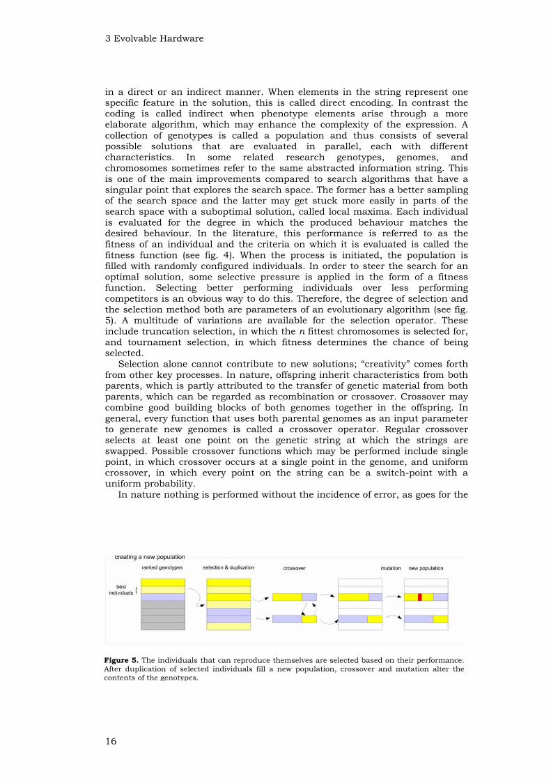
Figure 5. The individuals that can reproduce themselves are selected based on their performance. After duplication of selected individuals fill a new population, crossover and mutation alter the contents of the genotypes.

copying of genetic material and its conservation. This effect can be regarded as mutation of the genome and is a widely used operator in evolutionary algorithms. Its main function is to explore the search space and to avoid premature convergence of the population. In general, every function operating on one genome alone can be regarded as a mutation operator. In the case of bit string genome representations, stochastic bit flips form common mutation operators. Transfer of characteristics between both parents is subjected to probability (pcrossover) as well as the probability of an element being mutated (pmutation). Since most these mechanisms operate stochastically, a new population can perform less well than the previous one. As a precaution an identical copy of the best individual may be placed into the next generation in a process known as elitism.

These operators in combination with the selection pressure are repeatedly applied to drive the complete population to eventually contain increasingly better performing individuals. Each complete cycle is called a generation and is usually characterised by the average, minimum, and maximum fitness values of the individuals in the population. These measures are often plotted against the generations, to get an impression of the increase of the fitness over time. Such plots are called fitness graphs.

3.2.2 Genetic programming Koza [30] has a different perspective on how to formalize genetic information. Instead of generating bit strings that must be translated into functional entities, genetic programming (GP) produces tree structured entities to solve a certain task. Traversing through the tree structure is similar to executing a computer program. Information inside the tree is used to generate an ‘unfolded’ individual, which is then evaluated based on the task. Nodes within the tree represent the operators of the program and gain their input from the branches which represent the program data flow. Starting at the leaves, which are the inputs, the data flows to the root node of the program. By recombining sub-trees of the parental structures to evoke crossover implementation in the GP, mutation can also swap sub-trees or leaves of the tree. The size of individuals, in contrast to most GAs, is dynamic as two sub-trees exchanged between individuals are likely to be of different depth.

3.2.3 Evolution strategies An evolutionary algorithm developed by Rechenberg and Schwefel [50, 58], in contrast to both former streams, operates directly in the phenotype space. It is specifically designed for domains with real valued parameters that need be optimized. The approach has two vectors which are used to find optimal solutions. First, phenotype parameters constitute a vector of values to be optimized, the problem vector. The second vector, the strategy vector, contains the size of the mutations in the form of an n-dimensional normal distribution. Mutation is the main operator in an ES; it operates on both problem and strategy parameters by applying changes on or using the normal distributions. The problem vector is mutated by noise defined by the gausians in the strategy vector. The standard deviation and mean of these gausians functions also are mutated. Selective pressure is often strong and appear in two forms. One is the (p,c)ES, in which the new population is based on the best p out of all the children. Alternatively, the (p+c)ES is a sort of elitist strategy, based upon choosing the best p out of the complete pool of parents and children; the (p+c)ES.


18

3.3 Evolvable hardware principles But how can we link these evolutionary algorithms to search for electronic designs? Electronic components have complex physical properties that could be used in the evolutionary process. There is however an apparent trade-off between the freedom of the search algorithm and its ability to generate useable circuits. Current state-of-the-art electronics does not allow for the direct use of silicon material in the evolutionary process. Besides the enormous search space of possible configurations, the duration and cost to manufacture a silicon wafer for each individual clearly makes this an infeasible procedure. Common to engineers, circuits can be described at a higher level: schemas; the search space then contains genotypes that are transcribed into schematic configurations. Another common design principle is the use of truth tables to describe the function of digital circuitry, see the tables in appendix A for some examples. Genotypes are treated as bit strings for the output columns of those tables. Genes in the genotype are associated with electronic components that are rearranged through the process of evolution, which steers the component placement and routing.

In EHW a distinction is made between constrained and unconstrained and furthermore between extrinsic and intrinsic. Constrained evolution limits the freedom of evolution since not all possible configurations are allowed, for example recurrent connections. Unconstrained evolution poses no restrictions on the evolutionary technique to generate circuits. All EHW approaches that evaluate circuits in simulation are termed extrinsic evolution, when evaluation of individuals is done on physical substrates is termed intrinsic [16, 17]. Extrinsic evolution is often coupled with a constrained form of evolution, because feedback loops and such are difficult to simulate reliably and are computationally expensive. However extrinsic evolution is not committed to constrained evolution, since for example analogue circuits have been used in simulation (e.g. SPICE) without any constraints. In intrinsic evolution possibly unmodelled physical properties may be exploited. Therefore, this is commonly paired with unconstrained evolution where the most elementary building blocks of electronics are allowed to be altered by evolution [66]. Extrinsic combined with constrained evolution is clearly the easiest way to find circuits, but with several disadvantages. Simulation cannot incorporate complex dynamics. The discrepancy between simulation and the real world, can lead to the fact that evolved circuits in simulation perform less well on a physical substrate. Fortunately, the common availability of programmable devices provides a practical electronic substrate for intrinsic evolution. Most commonly known are the Field Programmable Gate Array (FPGA) [5, 80] and the Field Programmable Analogue Array (FPAA). The former is used to create digital circuits and has the advantage of supporting general description languages like VHDL, Very high speed IC Hardware Description Language [80], which allows for the implementation of circuits on FPGAs regardless of the brand. The latter, which is used for the creation of analogue circuits, regrettably lacks a similar general description language.

FPGA-like devices use configuration strings that determine the connectivity and modes of its elements. To use evolution for circuit design on FPGA like devices, genotypes are mapped onto the configuration strings. In most architectures each FPGA element contains a lookup table (LUT) that represents its output as a logic function of its inputs. Care must be taken in configuring, as some strings produce invalid or even damageable configurations, as random routing could produce short circuits in some architectures. The use of JBits as a wrapper around the phenotype may prevent damage to the circuit by potentially harmful evolved individuals. JBits gives an insight in how the mutated string relates to the routings between FPGA elements, and enables the

filtering of harmful individuals. FPGA devices can be reconfigured at runtime and have a large, or even limitless, amount of reprogramming cycles. This makes them very suitable for the intensive evaluation demand of evolutionary algorithms and widely used within the evolvable hardware community.

3.4 Evolved hardware One of the first milestones in evolvable hardware was laid by Tetsuya Higuchi, who, in addition to formulating a practical definition of EHW, presented the first evolved circuit on a GAL16V8 programmable logic device [24]. Since these devices have a limited quantity of reprogramming cycles, extrinsic evolution was used to evolve individuals. The final post-evolution individuals were tested on the actual hardware device. This limitation has recently been resolved by using FPGAs with an unlimited amount of reprogramming cycles. Initial populations were filled with individuals in the form of valid configurations and subjected to a GA to evolve successful individuals.

The first circuit was a 4-bit multiplexer; a non-trivial task since learning the topology of this circuit belongs to the NP-complete class of problems [42]. A population with a total of 64 chromosomes, each 108 bits, was used to successfully evolve such a circuit. Chromosomes with a slightly larger length, 157 bits, were used to evolve a 3-bit counter using a 0.5 percent mutation rate and a crossover probability of 60 percent; the whole evolutionary process took for about 200 generations to come up with a successful solution. A more complex 4-state machine needed 650 generations on average to appear in the population, using a 157-bit genotype, uniform crossover (pcrossover=20%) and mutation (pmutation=5%).

Around the same time, John Koza used GP to create boolean multiplexer functions [30, 31], in the form of an simulated 8-bit multiplexer. The transfer of this method to a hardware device is non-trivial due to the in advance unknown memory resources. This is the main reason why a GP is not often used in EHW as an evolutionary approach. To use a GP for EHW, the resulted tree has to be mapped into a placement and routing of components and is synthesised on a FPGA chip. The GP used 3 address- and 8 output lines as terminal symbols and used AND, OR, NOT and IF as the operators in its toolbox. Using 4000 individuals, a 90 percent crossover rate and no mutation, the GP produced successful individuals after 9 generations and was nearly converged after a total of 15 generations.

It was not until 1996 that intrinsic evolution was successfully used to produce circuits; Thompson [66, 67] used such evolution to produce a tone discriminator; the task was to discriminate a 1 kHz square wave from a 10 kHz version. Frequency discrimination can generally demodulate frequency modulated signals and decode the low frequency information; in this case it would produce a binary information string. The lack of a timing signal in the form of a clock or an attached RC-circuit makes the design difficult, and posed a challenge for evolution to come up with a good solution. As an additional constraint, the circuit was limited to a partial grid of 100 FPGA cells, leading to an 1800 bit sized configuration string. The circuit was directly encoded in the genotype of the 50 individuals in the population. A GA used a crossover probability of 70 percent and an expected amount of 2.7 mutations per genotype. The continuous input signal consisted of 5 occurrences of both the 1 kHz and the 10 kHz square wave signal in repeatedly random order. After 650 generations the circuit started to successfully discriminate 1 of both input signals. After 3500 generations, and 2 to 3 weeks later, the behaviour seems optimal. Analysis of the evolutionary history revealed that clusters, or species, arose prior to a performance increase. One of these ‘species’ in the population contains the solution that is further specialised through mutation.


20

During evolution unconventional behaviour is observed. This gives support for the hypothesis that intrinsic evolution explores outside the conventional search space. In addition it seems that evolution utilises the components differently from their conventional binary logic abstraction [67]. Seemingly unused components, in the sense that no functional connections are routed into them, surprisingly play a role in the behaviour of the circuit, probably due to electro-magnetic effects. While clamping some of these ‘unused’ cells to a constant value has little effect, others completely deteriorate the system performance (see fig. 6). The produced circuit is quite tolerant of frequency errors; the switch point between output states lays well past the first frequency point of 1 kHz. Decreasing the operational temperature shifts this point nearer to the middle, but excessive temperatures make the circuit fail to discriminate properly. Evolved individuals are specialised to this particular location on the grid. Transfer of the 10 by 10 grid to another part of the 64 by 64 grid on the same FPGA had varying negative influence on its performance dependent on its new location, while transfer to another FPGA device deteriorated its performance drastically.

To increase the complexity of circuits produced by EHW, Layzell [36] developed an Evolvable Motherboard (EM) that allows various more sophisticated electrical components to be interconnected via artificial evolution such as operational amplifiers, multiplexers or bipolar transistors (see fig. 7). Routing of all components is done by 1500 analogue switches, which is equivalent to a search space of roughly 10420 possible circuits. To prevent the short-circuiting issue seen in the first approach, each switch contains a small “on”-resistance. To aid the behaviour analysis of evolved individuals, each component is easily accessible by measuring equipment, in contrast to a FPGA device.

A basic inverting amplifier was evolved using the EM, while ignoring the possible phase shift or the overall frequency response. The population numbered 50 individuals and was altered via single-point crossover and a 0.01 per bit mutation probability. A restricted genotype mapping in constrained evolution limited the amount of local connections and lead to a 1056 bits genotype string. The removal of resistors and capacitors from the toolbox, leaving only transistors and analogue switches, made this task non-trivial for evolution. After 2000 generations, a functional but unconventional amplifier had come about; inputs are not connected to common connectors since transistor input was applied at the collector instead of the base.

Ricardo Zebulum et al. were the first to produce analogue circuits with the use of artificial evolution and field programmable amplifier arrays (FPAA) [79].

Figure 6. The intrinsically evolved tone distinguisher, note the grey boxes; while electrically not connected, clamping them deteriorates the overall behaviour [67].

Figure 7. The Evolvable Motherboard; an architecture designed to facilitate the evolution of more complex circuits.[36]

Electrical circuits are evolved using a GA and properties are encoded within a gene: connectivity, type and value per component. Their goal was to evolve an operational amplifier (OpAmp). Designing such a system involves optimisation of gain, bandwidth, slew-rate, power-consumption and noise. However, the focal point of evolution was to produce a typical DC response common for OpAmps. A collection of 15 genes, 40 individuals, one-point crossover and elitism produce a correct individual after approximately 90 generations in extrinsic evolution and performed almost identical in real hardware. Intrinsic evolution was used to produce a 200 kHz oscillator using a 300-bits genotype; coding for a configuration string for 2 cells of the FPAA. Successful evolution depended on the use of 40 individuals, 40 generations, one-point crossover and a 7 percent mutation rate.

In pursuit of evolving analogue circuits, Zebulum was also involved in the development of the Programmable Analogue Multiplexer Array (PAMA) [56]. Low-level components are connected via switches whose states are evolved using a GA, similar to the EM approach of Layzell. The simple architecture can incorporate any type of component. Like the EM it incorporates small short-circuit preventing resistors and its components are easily accessible with measuring equipment. The architecture is used to evolve well-known circuits: an XOR gate and a 2-bit multiplier. By using only a few components, n npn-transistors, m pnp-transistors, q resistors, it is possible to evolve both circuits. Later work showed that evolution can produce many inverter circuits, which are based upon designs uncommon to conventional engineers.

Efforts in the field of evolvable hardware have sprouted a wide variety of architectures. The Jet Propulsion Laboratory at NASA has developed a system suitable for both analogue and digital circuits; the FPTA (Field Programmable Transistor Array). Currently an improved FPTA2 has followed and also includes a visual sensor array and thus forms an evolvable sensor system. Jörg Langeheime et al. used this architecture to evolve logic gates: NOR, NAND, AND, OR, XOR and XNOR and inspected their quasi DC behaviour [35]. Successful evolution varied per logic gate, the NOR and NAND functions were easy to evolve. In the case of the XOR and XNOR functions, no suitable solution was produced. There is a direct relation between the evolvability of the functional gate and the required amount of transistors; XOR needs 10 transistors in order to function, a component count that appears to be too much for this approach.

3.5 Summary We have seen that evolution can be used to create unconventional designs, original design as compared to human designs. Also the automated process is sparse in terms of human intervention, only the definition of the fitness function and a hand full of evolutionary parameters are pre-defined. From this overview some preliminary conclusions may be drawn. The field of EHW has, to date, been littered with a multitude of scattered architectures, each with its own focal point. As a result of this, much of the research efforts performed up to this point cannot be compared and research efforts sprouted from them seem like ad hoc solutions for small problems at hand. A critical note with regard to these circuits must be made. While it is possible to evolve circuits with success, much is unknown about their operation properties outside the environmental envelope used during evolution. In order for these components to be useful, some guarantee about circuit operations must be provided, arguably in the form of mathematical analysis. Even within this operational envelope, the produced circuit is difficult to understand, as components can produce behaviour based upon unknown properties. Insight in the evolved behaviour may aid conventional circuit engineering in producing new techniques or


22

building blocks for use in future designs. Due to the difficulty of designing complex systems based upon these architectures, most research focuses on small building blocks. Although the work of Higuchi on these elementary blocks seems logical: all new research has to start at small understandable blocks, a decade has passed until then and research still seems to focus on these elementary blocks. Although the complexity of these blocks have increased, it seems unlikely at the moment that evolution will produce circuits far beyond these elementary building blocks. These problems have been classified by the evolvable hardware community into two key problems: scalability and evolvability. When a circuit needs more components for its functionality the genetic material scales quadratic and results in a huge search space; effort should be made into making this relation less costly and allow EHW to scale into larger applications, for example with growing circuits based on a genome: developmental encodings. Since evolution searches for a solution with use of a fitness landscape, smoother landscapes as a consequence of different genetic operators could also aid the evolutionary process and makes complex circuits more evolvable.

Chapter 4

Artificial Ontogeny 4

In nature we find growth all around us and ontogeny has inspired researchers to explore some of its fundamental principles. Developmental algorithms that grow upon initial structures are grouped in a research field called Artificial Ontogeny (AO). Additions of development-inspired notions into evolutionary algorithms can make them more powerful, as the evolved genotype is not directly mapped onto the phenotype. More complex problems may be expected to be handled, since the search for a good genotype takes place on much simpler structures [2]. Based upon these structures grows the phenotype, which makes the task evaluation less bound to the genotype. This may lead to interesting results in terms of scalability, since growth fundamentally lends itself for scaling.

4.1 Ontogenetic techniques Artificial Intelligence is either approached using the top-down or the bottom-up approach. The former tries to tackle problems by repeatedly subdividing them into subcomponents until all that is left are available building blocks which may be tied together. The other approach begins with low-level environmentally connected blocks linked to form loosely coupled systems [46]. Both approaches have advantages and disadvantages. The former approach is able to create complex structures and interaction in strict and formal worlds. The latter however, is able to deal with noisy and unknown environments and thus more suitable for embodied real world applications. We see this division reflected in artificial ontogeny, grammar versus cell chemistry based, although recently it has been challenged whether this breakdown should still be adopted.

Stanley and Miikkulainen propose a new taxonomy based on 5 properties, which better reflects the characteristics of artificial ontogenies (AO) [59]. The first property accounts for the way each element in the grown structure obtains its eventual state, the cell fate, and can vary between pre-patterning and self-organised. While some systems obtain grown states through a staged unfolding, others rely upon emerging effects that lead to stable end states. Targeting addresses the way each cell is connected to neighbouring elements; this is either relatively encoded or strictly specified. Relative encoding is particularly interesting for growing connectivity schemes, such as in neural networks. Development in biology usually occurs in a staged fashion, as changes in phenotypes are often clustered in time. Variations in these developmental plans can have a large influence on the final grown structure. The effect of changes in the developmental plan and insensitivity of the system related to these alterations is called heterochrony and forms another axis of the taxonomy. Mutations utilised in GA may be very damaging to the used direct encoding, this is contrast to biological mutations. The use of an AO may result in less harmful mutation operators for the phenotype. Cell fate is not predetermined by the genome, but arises out of a dynamic allocation that can compensate for genomic alterations. This flexibility is referred to as canalisation. The last point addressed by Stanley and Miikkulainen is related to complexity; the increase in

4 Artificial Ontogeny

24

genome length over time could lead to complex evolved individuals. So the inclusion of a variable length GA is an important aspect of an AO.

A complete review of all the work in the field of AO is beyond the scope of this chapter. Some main work will be presented to give a global idea of the state-of-the-art achievements in this terrain. Moreover, it reveals an indication about characteristics of these methods. As Dawkins stated [9], every AO approach is blind outside its own scope. Although AO increases the capacity of an evolutionary algorithm to grow structures, these phenotypes are extracted from an AO-specific pool and give rise to well-known characteristic phenotypes for certain AO-strategies. This does not necessarily imply a limitation, since certain AOs can be well-suited for specific domains.

4.2 L-Systems The development of plants and their highly repetitive structures were inspiration for the systems introduced by Aristid Lindenmayer [39]. At the basis of this approach are rewrite rules; a grammar is used to unfold the original string into a ‘developed’ or unfolded string. At the start the algorithm uses a seed, which can be conceived as the root of a tree. The seed is used as an input for rewriting rules. In principle, a rule can be applied when a non-terminal symbol in the string matches with the precondition of the rule. After the rule is applied either a terminal or a non-terminal symbol, defined in the post-condition of the rule, has taken its place. Repeated application of rules eventually leads to a string containing only terminals, reflecting a mature individual. This process can be regarded as growth, because the original small root string can be unfolded into a larger string.

L-Systems have the advantage of being easy to implement and quickly producing regular structures. The original concept has been expanded to allow for more irregular structures to emerge. Normally when a precondition is met, each rule is always applied. By adding a particular rule-probability, matching becomes stochastic and the introduced uncertainty caused produced structures to differ from each other. To enhance the expressive power of L-Systems, Lindenmayer added parameters to the rules: parametric L-Systems. This indirectly led to the use of context sensitivity; the applicability of a rule can vary throughout the structure. Matching rules depend not only on the present pre-condition symbol, but also on the compliance of its neighbourhood to the given conditions. Applications of all kinds of L-Systems are found in areas where connection schemes play an important role, especially in neural network

Figure 8. L-Systems typically grow tree like structures, usable for network connectivity schemes.

Figure 9. Reaction diffusion systems can produce bio-mimetic patterns through differential equations, like this ‘fingerprint’.


architectures. In addition, they have been used for the growth of virtual creatures, where they defined the placement of body parts.

As these branching structures resemble trees (see fig. 8), Hiroaki Kitano [29] was inspired to use this method for generating neural network architectures, and successfully evolve genomes which could be compared to direct encoding schemes. Several researchers developed upon this idea to grow connection schemes, and show that grammar encodings do not suffer from an increase in network size. This serves to make the evolutionary algorithm more scalable. Unfortunately, this method had been outperformed by later work which involved direct encodings. Renowned work in the field of artificial life by Karl Sims has shown that interesting and bio-realistic structures and behaviour can be evolved using L-Systems [59]. An important observed feature is the reuse of gene building blocks in order to produce the phenotype. Gregory Hornby and Jordan Pollack showed that evolving these kinds of creatures in real environments with this kind of developmental phase outperformed individuals produced by a direct encoding [26].

4.3 Reaction-Diffusion Systems The inspiration that lead Alan Turing to invent reaction diffusion (RD) systems was the intricate patterning on seashells and animal skin [71]. He abstracted these emerged patterns to the chemical interactions of long range diffused chemicals and locally reacting substances, hence the name RD-systems. At the basis of these systems are simple differential equations, which represent chemical behaviour. At each point in the environment, this equation describes the concentration gradient, which is a function of other chemicals and environmental parameters. In this way, chemicals can either enhance or repress the production of other chemicals in the environment. Over time these equations can transform the space in which chemicals initially appear in a homogenous concentration into complex structures. Initial conditions partly determine the resulting structure; other influences are equation parameters and noise introduced into the system. While it is fairly easy to generate patterns (see fig. 9), it is difficult to determine the precise parameters of the system required to generate a desired pattern. Often systems work with non-intuitive parameters and tuning them to a specific pattern is very difficult as grown structures rely for a large part on emerging effects.

Further work remains to be done in exploring the parameter space and its relation to the grown structures, if one is to use RD-systems in real applications. Nishimiya et al. have used a reaction diffusion system to create a chip with specific patterns emerging upon it [44]. Although it is feasible to create a minimalist RD-system to create patterns on a VLSI-chip, direct application for these grown structures are limited. However, it should be noted that RD-systems can grow a wide variety of structures; taming the beast into realistic, useable systems seems to be the motto for the next decades.

4.4 Bio-Chemical Networks Biological networks, as for example genetic regulatory networks (GRN) (the way genes regulate other genes) and metabolic networks, have properties that resemble other well-known network based systems, like artificial neural networks, electrical power grids and the World Wide Web. This resemblance aroused attention from researchers among various fields and brought to light that all share common properties: small world, scale free and small patterns [15]. Highly clustered networks are called small world networks if despite the sparse connectivity, every two nodes in the network are connected by at least one path.


26

Scale free is a somewhat related property; it states that the connectivity of each node is given by the power law p(k)=k-γ. In this case, the probability of a node having k connections is decreasing exponentially with k. Nature’s bias towards this can be explained by the combination of two processes, first networks continuously expand via the addition of new nodes, and secondly these new node prefer to be connected to the, already highly connected, existing nodes. In the case of GRNs, node duplication also occurs; large parts of the genome are transposed or duplicated to another part of the genome, which in effect makes an additional ‘node’ where transcription factors can bind and produce identical proteins. Consider a GRN in which nodes are states representing the necessary environmental condition (proteome) required for it to jump to another node. Mutation can alter some duplicated connections, which lead to specialisation of the duplicated node; transcription is initiated by a slightly different proteome.

Another well known feature in these networks is the occurrence of small recurring patterns in metabolic pathways or frequently appearing building blocks in bio-nets. In biological networks, a small set of basic recurrent patterns are identified as building blocks that give rise to the huge variety of complex interactions between cells structures found in nature.

It seems that when networks are characterised by these properties, they show robust overall behaviour when nodes are randomly removed from the circuit. The application of lesion to targeted nodes in the system can however have a severe influence on the system operation [18].

4.5 Random Boolean Networks To model the interaction properties of biological genetic regulatory networks, Kauffman introduced random boolean networks (RBN) based on binary cellular automata [28]. The notion of RBNs has been widely applied to various areas for modelling complex systems [19]. Like cellular automata, the system works with a collection of states and their transitions. Each state represents a certain protein mixture. The state transition determines the next state of the system for each current protein mixture. Proteins are abstracted in a binary fashion, and are either present of absent.

RBNs can be represented in 2 main fashions. The first is a connection matrix in every value relates to the type of connection between two states i and j: +1 for activation, -1 for inhibition and 0 for no connection. The second type of representation is creating a boolean logic function for each node. By mutating these representations the connectivity and the expression of the genes can be altered.

These systems are characterised by (n,k) landscapes, related to the number of nodes, n, and the quantity of connections arising one node, k. Main interest for these landscapes is the notion of attractors, which are a common notion in dynamic complex system design. When complex systems depend on previous states, complex temporal behaviour can emerge. These state transitions can be pictured by paths in a multidimensional space and their behaviour is categorized dependent upon these phase changes. When states fix to a single state, the behaviour of the system is forced to a single setting and is referred to as stable behaviour. If a system is constantly changing between random states, its operation is called chaotic and the system is challenging to utilize. When the behaviour repeatedly steps through a limited set of states, it is referred to as cyclic behaviour and can produce interesting patterns.

So next to creating spatial structures, it is also possible to create spatial temporal structures, which can be utilized when operating in temporal domains. This is quite common when working with real world problems obviously.


4.6 Genetic Regulatory Networks Regulation of genes is one of the principal means that induce cell differentiation, essential to producing structural diversity in an organism. This phenomenon is widely studied by biologists and computer scientists and is simulated in several levels of biological realism [8]. In the area of cell modelling, these networks are used to simulate cell interactions and “life cycles”. While these complex models lack applicability to real time applications, efforts into making minimal genetic regulatory networks have lead to promising results.

In a GRN, genomes are divided into genes that can be unlocked when cell environmental requirements are met, which is similar to reality (see chapter 2). In general, proteins in a cell may bind to specific regions that are related to genes. Bounded proteins can either lead to production of the protein type encoded by the gene or cease protein production. The former is referred to as an expression or activation and the latter as an inhibition relation. This relation is encoded in the genome, as it encodes which protein type can bind and which protein type is produced. The complete system is situated in a simulated environment in which proteins can exist in various concentrations. Since the proteins in the system act upon the genome, these protein concentrations and a genome are paired within the cell system. Multicellular GRNs contain multiple copies of identical genomes and allow proteins to be diffused between cells, although a lot of current research is restricted to a single cell.

In most cases, protein concentrations have to be beyond a genetically encoded threshold for the gene to be ‘unlocked’. Protein concentrations vary over time due to their decay and diffusion within the system. Protein types in a system may vary in their half-life and this limits the temporal effect of produced proteins. Diffused proteins flow from cell to cell and may also vary per type in their ability to reach nearby cells. In this sense the system may exhibit temporal behaviour due to production and decay. Diffusion in a multicellular system can lead to spatial patterns, as protein mixtures may determine cell functions.

4.6.1 GRN research Genetic regulatory networks have been used for a wide scale of applications. Historically applying this method for developing the connection scheme for neural networks is the most obvious. Eggenberger used GRNs to create cellular small structures (see fig. 11) using cell division and cell differentiation, both of which were initiated by the regulatory genes [13, 14]. As in all GRN related work, he used transcription factors that can bind to specific domains on the genome. In order to form structures, individual cells must be connected. Special proteins, so called cell adhesion molecules, are produced by the GRN. The matching of cell adhesion molecules between two cells determines the availability of a link. The sigmoidal neuron cells are formed into a network topology and are used for a combined obstacle-avoidance and light-source tracking task on a Khepera robot.

More complex embodied behaviour was produced by Bongard [3, 4], who used GRNs to create virtual creatures (see fig. 10). Unlike most related work, his GA works on variable length genomes consisting of floating point numbers. Evolution was used to produce both controller and morphology. The controller consisted of a complex network in which neurons are connected with the sensors and the actuators of the creature. Creatures are formed out of structural blocks, the basic building blocks of the organism. Within each unit, expressed genes determine the full functionality of the block. Gene products are assigned to cellular operations like, cellular division, synapse adjustments and changing the neuron type. After 200 generations and a growth period of 300


28

time-steps per individual, successful block-pushers and other interesting morphologies emerged.

The temporal nature of GRNs is reflected in the work of Quick [49]. In his work, GRNs were coupled with the environment in several different tasks. Various gene lengths were utilised in a single cell environment, BioSys, which communicates via proteins. Heaters must compensate for deviation of an environmental temperature to a set optimum. By regulating temperature and heating level with proteins, an evolved GRN is able to maintain the environmental temperature at the optimal setting. Although this problem could be evolved with only 1 gene, increasing the genome length to 5 increases the success rate of all runs to 100 percent. A similar setup involving two genes allowed the successful evolution of light-tracking behaviour using a khepera robot. In this case, protein types were directly related to either sensor input or motor output speeds. Compared to direct encodings, we see that the fitness graphs do not increase smoothly. Large plateaus of equal fitness are ended with a sharp increase that takes only a few generations. This is associated with indirect geno-phenotype mappings and is related to the phenomenon of punctuated equilibrium in natural organisms [23].

Reil introduced Artificial Genomes (AG), and focused on the temporal aspects of the gene expression [51, 52]. Artificial Genomes use ‘spiders’, small active search units that scour the genetic material for genes. This in contrast to most other related research in which genomes are subdivided into pre-specified areas. A protein can bind to certain matching regions, and upon binding, it scans the following genome sequence until it finds a global specific sequence, 1010 in this case: a TATA-box like equivalent (a small region that marks the start of a gene), the succeeding n-digits are then treated as a gene and are transcribed. As in the RBN work of Kauffman, he distinguishes three kinds of gene expressions; ordered, chaotic and complex. Ordered gene expression occurs when the degree of regulation is low: genes are constantly active or inactive during the whole growth period. Chaotic expression is observed when genes are activated at random. But, as Reil states, the most interesting part is when gene expression shows a continuous temporal pattern, in which genes can be regarded as limit cycle attractors.

Watson used these artificial genomes and applied biologically realistic mutation operators to study their effect [76, 77]. In nature, in addition to single point mutation, two other mutation operations often occur. These mutations are transposition, or the relocation of a genomic subset, and tandem duplication, or the duplication of a genomic subset. The AG encoded the

Figure 10. GRNs used by Bongard [3, 4] to evolve the morphology and controllers of virtual creatures.

Figure 11. Morphogen induced structures; each cell reacts differently on concentration of the diffused chemical [20].


information to aid the growth of a tree like structure with the use of an L-System. While single point mutations of the AG had little effect on the grown tree, tandem duplication quickly became drastic to the phenotypic appearance. From this it appears that in terms of canalization AGs are quite well performing.

Geard and Wiles introduced a network approach to gene regulation, in extension of the RBN approach, which uses boolean relations between regulated genes. They increased the complexity of this connectivity to a sigmoid type, similar to artificial neural networks [18]. In this case, genes were not activated merely by the presence or absence of a specific protein mixture composition, but just like ANNs, the activation of the gene is based on the similarity of the proteome to the encoded ‘weights’ connected onto it. Using this method they were able to evolve a biologically pattern of cellular division and differentiation similar to a real organism.

Bentley and Kumar developed an Evolutionary Developmental System (EDS) in which they evolved growing embryos that incorporated directed growth [34]. Specific genes trigger effects such as cell division (mitosis) and cell death (apoptosis) and the spindle that controls the growth direction. In their model, they used a gausian protein distribution around the source of protein generation to model the diffusion of the produced proteins. They characterise their gene architecture as cis-trans regions; multiple binding-regions need to be activated to produce an encoded protein. They use this method to grow elementary spherical structures, clearly a typical solution from the search space defined by this kind of AO.

Gordon is pioneering in the transfer of GRNs to on-chip EHW. With a minimal model he succeeded in creating a pattern that serves as a template for an adder circuit [21, 22]. Gene encodings are similar to logic functions that determine to generate the output protein when the function is met. First approaches only included absence and presence of proteins as basis to produce their target pattern. Experience brought them to the extension of inequality and a slightly more advanced manner of intercellular communication: each cell detects every protein generated in its neighbourhood. Future work in this field should address the growth of more complex and larger patterns. The current model is designed for static patterns only, whereas temporal patterns may be very practical. As scalability is an important issue in the EHW field, measurements related to this topic should be addressed in future work.

4.7 Summary Artificial Ontogenies can grow structures each having its own characterised properties. L-Systems produce tree-like structures that aid the construction of network topologies, reaction diffusion systems are hard to tackle but create a wide variety of repeating spatio-temporal patterns, and gene regulation networks resemble the growth process of cellular structures, and often produce spherical structures. Complex models incorporating artificial ontogonies can bring an insight in cell biology. However, these complex models are unsuitable for practical applications. Minimalist models are less biologically realistic, but with the advantadge that they are suitable for practical applications. Artficial Ontogenies can have applications in designs of structures like robot morphologies, architectures and network topologies. Besides these spatial structures, some ontogenies can be applied for temporal control, like temperature control and robotic behaviour. Ontogenies however are usually implemented in a computationally costly complexity. Moreover, the application of AOs has been mainly focussed to software simulations, and research in this field outnumbers related work in the hardware field. In order to bring ontogeny to hardware substrates an effort in


30

minimizing the computational complexity of AOs has to be made. Hardware platforms incorporating ontogeny may open new possibilities in the fields of fault tolerance and robotic control.

Chapter 5

POEtic Tissue 5

Given the novelty of the bio-inspired POEtic tissue, it becomes clear that designing systems upon it is a pioneering event. POEtic tissue is designed to be a suitable architecture for evolutionary (P), growing (O), and learning (E) hardware systems or combination of the above. Genetic regulatory networks are an implementation of the PO-model. They combine an artificial genome with growth that arises through proteins that bind and diffuse. It has the additional feature to add the E-layer at later time, such as in the form of learning neurons.

5.1 POEtic architecture Restriction of adaptive hardware to one particular developmental axis made it unable to profit from possible synergetic effects of the combination of multi-dimensional development. POEtic tissue provides a common framework that allows researchers to devise bio-inspired systems that operate on multiple axes [55, 63, 72]. This in overall gives rise to an electronic substrate ready for original circuit design, self-repair and learning by interacting with the environment.

The tissue is implemented on a specially designed real-time reconfigurable FPGA-like device (see implementation details). Like all biological systems, this substrate has a multi-cellular nature; each cell contains an identical copy of the genetic material and can communicate with its neighbours via several communication channels, simulating either chemical or electrical pathways. Each cell can be an implementation of a subset of all three axes in order to study a PO, PE, OE or POE type of interaction for certain applications.

In the POEtic architecture, each individual biological model has its own separate layer (fig. 12), which provides the advantage that researchers are not burdened by implementing all three layers when they are only focusing on a single method. Other layers can be based upon compatible research and the overall behaviour results from the interaction of all layers. The genotype layer of the tissue stores the genetic material subjected to evolution. This forms the phylogenetic part of the development of a species. The genome of an organism is used as basis to grow an organism, using a mechanism that is located in the mapping layer of the architecture. During its lifetime, an organism, expressed in the phenotype layer, is allowed to learn by use of the implemented epigeny model. This could be one from a wide range of different entities, for example spiking neural networks.

5.1.1 Phylogeny POEtic tissue incorporates phylogeny in its genotypic layer, which contains the basic parameters that are subjected to the evolutionary algorithm. These parameters are divided into two main parts. Parameters specific to the application in question are grouped in the cell, used to initialise the implementation. For example when evolving neural structures these operators

6 POEtic GRN Cells

32

might be initial connectivity strengths and other related parameters. Moreover, the behaviour of cells is the result of intercellular interactions and the characteristics of this interaction are also part of the genetic process. One possible implementation uses a differentiation table to determine how signalling information encodes the type information as in the mapping of protein mixtures to cell types [53]. The differentiation tables of all cells can be accessed through dedicated connections by the evolutionary algorithm. Evolutionary mechanisms will adjust the table, rather than the complete set of operators. This separation may provide a more compact structural representation increasing the evolvability of the system.

5.1.2 Ontogeny Cellular differentiation plays an indispensable role in ontogenetic development and thus can also be implemented in the multi-cellular POEtic tissue. Located in mapping layer of the POEtic tissue is the mechanism related to both cellular differentiation and division. In its basic conception, this layer determines the cell type with use of the differentiation table from the genotypic layer and is used to classify elements in the phenotype layer. The addition of this layer has a great influence on the expressive power of the genome. Similar to the proteome, this layer can transform static genetic material from the bottom layer into more complex and dynamic biochemical inspired structures and networks.

5.1.3 Epigeny The environmental interaction is most apparent in the phenotypic layer, and therefore is the most task-dependent layer in the tissue. Entities here interact with each other and the outside world to produce the desired behaviour. Sensory feedback to the tissue serves as a signal for both the mapping- and phenotype layer and can drive either the growth or learning algorithms. Various types of entities are suited for implementation, including, but not limited to, spiking neurons.

Figure 12. The POEtic architecture: each layer has a separate developmental axis associated to it (left). Researchers can focus on specific axis of the model, for example a PO system (right). On the implementation level these layers are mapped together and from a cell including these layers.

5.2 POEtic hardware POEtic tissue is a standalone device, meaning that evolution can run directly on-chip and as such provides a fast way to evolve systems. The complete tissue is divided into two main parts: the environmental and organic subsystem. The environmental subsystem controls the interaction between the outside world and the adaptive circuitry in the organic subsystem, and in addition controls the communication with several other chips that may easily be combined to form a larger tissue. A custom 32bit RISC microprocessor within the environmental sub-system is assigned to the execution of the evolutionary algorithms, the communication with the environment, and the configuration of the organic subsystem molecules. To suit the non-deterministic evolutionary algorithms, the generation of random numbers is implemented directly on-chip. An emulator of this microprocessor is publicly available1.

5.2.1 Organic subsystem Cellular organisms are not surprisingly composed out of cells, which on their turn consist out of molecules; basic elements of the POEtic tissue (see fig. 13). As part of a larger structure molecules and cells are required to communicate with each other, which is promoted by the division of the organic subsystem into two layers. The molecules of the circuit lay in a grid; on top of this situates a layer of routing units facilitating intercellular communication (see fig. 14).

5.2.1.1 POEtic molecules Molecules are connected to four neighbours and a corresponding unit in the routing layer. They may operate in different modes. Each molecule has a one bit memory in the form of a flip-flop (DFF) and a 16-bit look-up table (LUT), utilised in different ways dependent on its mode of operation. In the 3/4 – LUT mode, the 16bit LUT is used directly as a look-up table; its contents map the 3 or 4 inputs to a single output bit and can set the internal DFF to a specific state. Information storage or the generation of timing signals can be produced using the Shift Memory mode; bits are shifted through the LUT in a one-directional manner; the most significant bit shifts out and the input bit replaces the least significant bit of the 16bit word. Two other modes, the Input and Output mode,

1 The microprocessor emulator can be found at http://asl.epfl.ch via the electronic

tissue research page.

Figure 13. Molecules are the basic element in POEtic based structures; they form cells and on their turn the complete organism [63].

Figure 14. Molecules reside in a flat layer and on top is a layer of routing cells, which provides inter-cellular communication.

6 POEtic GRN Cells

34

provide gateways to the routing plane and can communicate with each other via dynamic routing. The remaining modes include a Configure mode to reconfigure neighbouring cells in the tissue.

As self-repair and growth is an important feature in the POEtic tissue, organisms must be able to configure the cell type of spare cells and incorporate them into the system. Molecules can alter the configuration of neighbouring molecules, leading to structural growth and adaptation. Contained within a molecule are five blocks of configurable information, a LUT, the input selection of the LUT, a switchbox, the specification of the operation mode and some miscellaneous configuration bits. These blocks can be set by the microprocessor located in the environmental subsystem, but can also be altered by molecules themselves. The switchboxes take care of the connections from each molecule to the other units in the cell. The limited capacity of the switchbox ceils the amount of connections through it, so care has to be taken during design to prevent congestion.

5.2.1.2 Routing layer The information flow between neighbouring molecules is implemented directly on the bottom layer, and forms a static path between molecules inside an implemented POEtic cell. In most conventional FPGAs it is not possible to adjust routing in a random way due to the risk of short-circuiting. In POEtic tissue a special type of multiplexers is used to prevent short-circuiting, thereby removing the restriction on the routing- and evolutionary algorithms.

Long-range communication routing between the cells of the tissue is implemented on the top routing layer (see fig. 14). With conventional FPGAs the intricate connections can not be changed without the need for a computer to repeat its intricate routing process. In POEtic tissue, each routing unit can create connections at runtime in a distributive fashion [65]. Cells therefore can ask the routing layer to build new connections whenever necessary; one could imagine the addition or removal of cells due to cell duplication or death. This functionality is unique in POEtic tissue and is unseen in any commercial FPGA device. In this fashion, cells can pop into the centre of the tissue somewhat similar to its biological counterpart.

5.3 POEtic design In this work evolution indirectly designs POEtic circuits by searching through the parameter space for suitable initial configurations (like initial synaptic weights), human design skills are still required to produce the circuitry that forms the basic cells (see Appendix A). Consequently, convenient design tools are required. Yann Thoma produced a GUI to aid the configuration and routing of molecules and makes it possible to create POEtic based circuitry. To verify the expected behaviour of the circuit, the program can link to a simulation environment, ModelSim, and can step through the operation of the circuit one clock cycle at a time. Beyond the scope of this work is the possibility of evolving the molecules in a more similar manner as the work presented in the EHW chapter. This way, cells can be evolved and used in the multi-cellular POEtic tissue.

5.4 POEtic research Back to the global picture… We have presented POEtic chip hardware and the cell architecture, which allows for the combination of phylogeny and ontogeny. In this combination, genotypes are mapped onto a phenotype and are allowed to grow (see fig. 15). This combination has been a major point in the predecessor of POEtic tissue, the Embryonics project [40, 45, 48, 57]. Of this

research, the BioWall is probably the best known example. Cells inside this wall could be damaged and cellular repair mechanisms would compensate for the injury. The POEtic project however is more sophisticated, as cells can benefit from two additional forms of adaptation: evolution and learning. Moreover, cells in the POEtic tissue may have various sizes, due to the dynamic routing that can connect cells together at runtime. Roggen [53, 54] used a morphogenetic mechanism to map the genetic material to cell states through chemical diffusers. Morphogenetics is a process involved in the determination of cell types. We have previously discussed that cells differentiate due to available proteins in the local environment. This process can be modelled using diffusers, which spread signalling molecules that are used to define the cell types. This morphogenetic model is divided into two subparts, a signalling phase followed by an expression phase. During the signalling phase, diffuser “molecules” are transmitted, and fill the grid with concentrations of diffused morphogenes. Several types of diffusers are available in the system, each able to diffuse a certain morphogene from a set of four available variants. The expression phase utilises an expression table to determine the cell type according to the mixture of present diffuser molecules. Cells in the tissue acquire a function assignment via this process. In this case cells are in fact spiking neurons; each function is essentially the interconnection scheme for each neuron, thus the resulting structure resembles a network configuration, synaptic connections together with synaptic signs. The genotype used encodes the location of the diffusers in the grid as well as the assignment of functions to concentration mixtures in the expression table. In order to determine whether indirect encodings are outperforming the direct approach, the same experiments were performed using direct encodings. These experiments show that indirect encoding schemes perform better with regard to the maximum fitness and the speed at which this level of performance is achieved.

Figure 15. Each genotype is mapped onto a phenotype and allowed to grow for a certain amount of time. During this growth period, the fitness value is determined and stored, to produce an average fitness value over time that is associated with the genotype.

6 POEtic GRN Cells

36

Chapter 6

POEtic GRN Cells 6

With prototype chips still under construction at the time of writing, design and experimental results are based upon other substrates. For the experimental results, a special simulator has been developed to mimic the final GRN cells. This allowed for a versatile playground to experiment with several implementations of the gene regulation and diffusion mechanism. This experience led to a POEtic-hardware based GRN cell with minimal properties to allow for essential regulatory operation: regulated production, diffusion, and decay [3, 12, 22, 33, 49]. The reason for this strip-down is obvious; although the substrate is flexible, space constraints and sparse integer communication are major points to address.

6.1 GRN cell behaviour In a broader sense, genetic regulatory networks are a subset of cell-based systems. In this broad class of systems, reaction and diffusion specifications play major roles in the produced behaviour. In reaction diffusion systems chemical concentrations are floating-point values and slight adjustments upon them at the beginning of the process can have severe consequences on the produced patterns. In hardware it is obvious to make such values discrete integers, either due to space or time constraints or both. In our simulation, we have therefore chosen to limit to integer values between 0 and 127; 7bit numbers. In order to apply diffusion and decay, a similar range of integers is scaled between 0 and 1 after multiplication to produce pseudo-floating operations.

In simulation all cells are evaluated in serial, in contrast to the parallel operation on the hardware circuit. A snapshot of the current proteome, the protein concentrations, per cell is made onto a second tissue, which stays

Figure 16. The environment infuses proteins in the tissue at pre-defined injection-spots, which can happen at any time during the growth period. At each time step every cell diffuses its protein concentration based on evolved diffusion rates. Proteins also decay based on evolved decay rates.

6 POEtic GRN Cells

constant during the growth period and serves as an input to all processes, leading to a similar behaviour. The tissue is evaluated for a certain life time, and can grow certain patterns as a result of the protein interaction; we refer to this as the growth period (see fig. 16). Before this whole process, the proteins are decayed by evolved decay rates, which remain constant during the whole generation. At each cycle in the growth period the environment is allowed to infuse certain proteins into the tissue, at certain cells: injection spots and are inserted into the protein-concentration table of the corresponding cell. Regulation is thus based on the decayed proteins of the previous cycle and the currently environmentally or intercellularly infused proteins. During the cycle this proteome interacts with the genome to produce new concentrations of proteins, which are stored into a temporary protein table. This regulation process is repeated for all genes in the genome. In this multi-cellular system, proteins can diffuse to their neighbouring cells thereby altering their proteomes. Evolved protein-type specific diffusion properties are stored in a diffusion-rate table and are used to shape the diffusion interaction between cells. Since all described processes place their protein residues in the working memory, the temporary table, the protein table is filled with the new computed values at the end of the cycle.

6.1.1 Regulation A wide scale of regulation encodings and principles could be used in a simulation system like the one described above. We started with various implementations and eventually focused on a few of them. In all implementations hardware feasibility was the most important design criterion. All followed the basic principle of gene regulation, wherein specific sites in the gene encode for the protein that can be bound on it and thereby unlock a certain gene. Included in these regions is the threshold concentration of the protein in question required to activate the gene. To ease the regulation process, a linear relation between available proteins and produced material is used. Protein production is biased by genetic encoded levels: beyond this boundary production of proteins is cancelled. Within them produced protein concentrations are determines linear on the biased concentration of the binding proteins (See regulation mathbox). Another common simplification is the use of direct matching; the encoded type has exactly match the type of the contained protein type. Literature suggests the use of a template based encoding, but

Math Box Regulation The minimal level encoding has 4 main fields that determine the protein production: a cis-region encoding the unlocking protein type: cis, a bit indicating whether the gene-type either is inhibitory or activory: i, the critical protein concentration at which the gene starts producing proteins: min and the protein type that is produced by this gene: prod. In this notation, Px is the concentration of protein type x. (Eq. 5.1)

=−=−

=0)0,max(min1)0min,max(

iPiP

Pcis

cisprod

Eq. 5.1

The minmax level encoding (Eq. 5.2) has 1 additional field: a field that determines the maximal critical protein level at which the functionality of the gene stops.

>=−<=−<=−

=max&0)max,max(min&0)0,max(minmax&1)0min,max(

ciscis

ciscis

ciscis

prod

PiPPiPPiP

P Eq. 5.2

6 POEtic GRN Cells

38

eventual hardware constraints force us to exclude this for the moment [14]. We experimented with some different encoding types based on a biological background that are minimalist and hardware friendly at the same time. We used these encodings in the environment as described above.

6.1.1.1 Minimal level encoding One of the most compact gene encodings consists of 4 main regions. Primarily, a gene must specify the protein to which it is sensitive; we refer to this as the cis-region, although literature has several analogous terms for it. An activated gene produces a certain protein encoded in one of the other gene regions. The relation between these two proteins is determined by the remaining two regions. Not only is the presence of the binding protein informative: a gene is expressed once the protein concentration reaches the threshold encoded in the genome. A single bit toggles how this threshold should be interpreted; the gene is either specifying an activory or inhibitory relation between proteins. Either it produces proteins when stimulated above the threshold or ceases to stimulate respectively. In total each gene of this encoding consists of 12 bits.

6.1.1.2 MinMax level encoding This encoding is a less biological plausible abstraction of the mechanism found in nature; to allow for more precise adjustment to the protein-concentration an extra protein level is added. The added maximum cuts off the activity induced by the promoter protein of a gene when this reaches the encoded certain level. The other common properties are utilized in a similar manner as with minimal level encoding. In total each gene of this encoding consists of 19 bits.

Math Box Diffusion Proteins are decayed dependent on a gradient of the current concentrations, first the gradient is determined for all neighbours i (Eq. 5.3) and then this is added to the current cell j and simultaneously scaled by the diffusion rate for each protein type (Eq 5.4).

jc

ic

ijc PPP −=∇ Eq. 5.3

∑∇+=i

cijc

jc

jc DPPP Eq. 5.4

After this all, the diffused proteins are lost from this cell; therefore the current concentration has to be subtracted by the diffused proteins (Eq.5.5).

∑∇−=i

cijc

jc

jc DPPP Eq. 5.5

Presented here is an example of the hardware friendly diffusion mechanism, for one protein type and one time step. The diffusion rate is set to 0.2 for this particular protein type.

6 POEtic GRN Cells

6.1.2 Decay Proteins do not stay in the system forever, like biological material they degrade over time. In order to improve the evolvability of the system, each protein-concentration is adjusted via genetically determined decay rates. In a first series of experiments protein decay was fixed and posed a serious problem for the evolution of patterns. For each protein type in our system evolution determines whether it is a long-lasting or a brief one. At each time step a decay rate between 0 and 1, dependent on its protein type, scales the protein concentration. In effect this lets protein types operate on different timescales.

6.1.3 Diffusion In this multi-cellular system, each cell is able to influence their direct neighbours. POEtic molecules, and thus composed cells, can signal to their four neighbours, to the north, the south, the west and the east. It should be noted that due to the unbounded nature of the GRN-tissue, each cell in the right column is connected to the left column and vice versa. A similar connectivity is applied at the bottom and top rows of the tissue. This type of connectivity was chosen based upon experience with reaction-diffusion systems, in which patterns rely on this unbounded feature to emerge. In the case of POEtic tissue, communication is based upon “proteins” transmitted from one cell to another cell. As in nature, transmission comes at a certain cost. Not all released messengers/proteins successfully make it into the neighbouring cells. Within the diffusion mechanism, a diffusion rate determines the transfer success of a transmitted protein. High degradation of a certain protein type leads to locally operating proteins and allows for spatially high frequent structures to emerge. On the other hand, low degradation allows generated proteins to travel through a higher number of cells and thus influencing a large part of the tissue at once, especially convenient to trigger background events. Diffusion is steered by gradients, high potentials leads to flow, while zero potential results in no flow at all. In our case, diffusion is also influenced by protein concentration gradients in the tissue (see diffusion mathbox).

6.2 Simulated GRN cells In absence of the final chip, as previously stated, experimental results have to come from simulated tissue to this date. To this end, a simulator mimicking the properties of the GRN cells, diffusion, regulation and decay had to be designed. Tissue in software simulation provides a pliable environment to experiment with effects brought about by diffusion and regulation. Inspiration from similar research in light of the abilities of POEtic tissue led to usable GRN cell models characterised by elementary gene regulation behaviour (see fig. 8). Several of these implementations were chosen to be subjected to evaluation of their performance on various tasks. As a main objective, the software has to fluently produce experimental results for a variety of tasks. A special batch mode is included in the program to run several experiments with different settings without human intervention.

6 POEtic GRN Cells

40

The object-oriented program is written in Java and is spread over several packages, each with its own functionality: evolutionary engine (ea), cellular environment with a separate part for the variety of cell types (env), a graphical user interface (gui), the collection of tasks (task) and some additional utilities (util).

Simulated data is not processed within the application, apart from fitness data all sorts of data could be exported to data files for analysis of protein interaction, decay- and diffusion rates and images of the produced behaviour. Analysis of this data is done in MatLab; scripts are written to produce all kind of statistics based on these output files. More details about the software implementation can be found in the included appendix.

6.3 Hardware implementation Simulated cells are convenient for deriving experimental results, but to show that this PO model is portable to hardware the same mechanism has to be translated in POEtic molecules. This POEtic based cell can be used in intrinsic EHW experiments. Since we also have space limitations due to the small size of the initial prototype, we had to be careful to design a proper POEtic GRN cell. Consider the fact that the first prototype consists of approximately 200 molecules per chip for the organic subsystem. The exact size depends on the amount of genes in the cell, as they are included in a separate memory module of the system. The hardware implementation operates on each gene at a time and makes the amount of genes variable. The current design is targeted for 4 proteins, which is a constraint of the system, extending this requires a complete redesign of the implementation. At present, one chip could contain approximately 1 GRN cells and larger cell grids can be created by combining several chips together, which is possible in a transparent way with POEtic tissue (see fig. 17a). Given the fact that our minimal level encoding seemed to perform quite well in simulation (see experiments in the next chapter), its low space requirement made it a logical candidate for hardware implementation. The current implementation includes

In digital circuitry design the choice between serial or parallel implementation is quite common. Serial versions have the advantage of being friendly in terms of space, however rather costly in time, vice versa for the parallel implementations. Our most prudent constraint is already stated, and therefore we chose for a purely serial implementation.

Due to the novelty of POEtic tissue, even elementary building blocks like addition or multiplication still had to be designed. Fortunately, only a limited set of such blocks were necessary for our GRN cell. Complete descriptions of the building blocks are given in the appendices of this thesis.

Figure 17. (a)An overview of the model we present in this work; POEtic based cells, each of them containing an identical gene regulating mechanism. (b)Proteins can flow to the neighbouring cells to be added to their proteome and play a role in the regulation, decay and diffusion pathway.

6 POEtic GRN Cells

Each cell contains a complete genome, as this is one of the key points in the POEtic project. This is contained in a collection of memory cells which can be cycled through and selected by a common multiplexer. Each of the genes contained in the genome is processed in serial and is allowed to produce proteins and as such influence the neighbouring cells. Each gene is parsed and thereby reveals the protein types related to it.

Each cell had two memories of protein concentrations. One is the main memory, and the other is a working memory used during protein production and diffusion. Data flows between these memories through serial pathways that compute the new concentrations for the next time step, each of them processed in serial (see fig. 17b). For more information about the hardware implementation, see the appendix on hardware details.

6.3.1 Decay pathway Inside the cell is a table containing evolved parameters, the protein decay rates for all available types. Each entry in the protein table is cycled through and scaled by this value; first multiplied by the scalar and divided by a 7 bits shifter, similar to a division by 128.

6.3.2 Regulation pathway The cis-region produces an address for a selectable memory cell; this outputs the current concentration, which is compared by a switch-able comparator that also has the minlevel and an inhibition bit as an input. Its output, the biased value, is added to the temporary protein table, which points to the entry directed by the production region in the gene. Since this pathway expresses only one gene at a time, all genes are cycled through before proceeding to the next pathway.

6.3.3 Diffusion pathway The most intricate and space consuming pathway involves communication between neighbouring cells. Each current protein concentration has to be scaled by diffusion rates stored within a table and transmitted to neighbouring cells. At the same time it has to process received concentrations to the current concentrations.

7 Experiments

42

Chapter 7

Experiments 7

Genetic regulatory networks have been mostly used for creating systems that can grow and develop structures in space. Since the proteome in a single cell, created from the genome, behaves dynamically due to infused proteins from neighbouring cells and external influences, it is also possible to generate spatial-temporal patterns. Furthermore, this temporal nature could also make the tissue somehow fault tolerant. As the functionality is not directly encoded in the genome, but comes forth from the interaction of produced proteins, complete structures could be more temporarily stable when parts of the tissue fail to operate properly and are compensated by internal dynamics. Patterns determine circuit functionality and pattern stability is directly related to the system fault tolerance.

Simulations addressed the basic capabilities of the GRN POEtic tissue; how it is able to grow structures, how it reacts to induced faults, how it is able to perform temporal behaviour, and how it could be used in robotic applications. In addition to viewing its behaviour in isolation, comparing this method to direct encodings shows how it performs in terms of scalability.

The association between previously presented electronic circuits and the work presented here can seem to be quite hard to make. As POEtic tissue aims at creating bio-inspired EHW, the eventual use of the tissue is not necessarily related to amplifiers or similar typical electronic blocks. Applications of these evolved structures could also be seen in higher level applications like neurons or oscillators. However, as the system is still implemented in hardware and eventually evolved, it may still be regarded as evolvable hardware.

Figure 18. (a) The temporal auto-correlation of the whole expressed tissue. Red means high auto-correlation, blue none, and while true random patterns only would have correlation at time index 10, (since the signal from a growthperiod of 10 steps is then compared to itself) we see that patterns are correlated even at more points in time. When shifted versions still match, we have a repeating signal: oscillation. (b) Generating a row in the figure (a): the history of one cell is auto-correlated and produces a row indexed by the delay index k.

7 Experiments

7.1 Auto response In the absence of a detailed description of an electronic circuit it can be difficult to analyse its behaviour. One method to obtain a functional description is by applying noise on the input and look at the produced signal; this leads to the familiar frequency responses of electronic filters. A similar method was also applied here, since the complex interactions of the system could lead to some interesting autonomous responses. All of the cells were infused with a random burst of proteins, leading to a random initialisation of the proteome. In addition the genome was composed of a random string, which was parsed in either the minimal level or the minmax level encoding. After this the characteristics of the systems can be derived. Analysis indicated that in the spatial domain, no clustering formation took place. However it seems that checkerboard patterns on the tissue are frequently generated. In order to inspect the temporal behaviour of the cell-tissue, an auto-correlation is performed on the history of the protein concentrations (see fig. 18). From this analysis it seems that random systems easily produce oscillating behaviour with an oscillation period of 2 cycles, essentially a repeatedly on-off behaviour. Figure 18a shows auto-correlation at various delay indices, which points out that protein concentrations repeat over time and is an indication for oscillations. In general the system easily produces checkerboard patterns in which the cells are repeatedly switching their states on and off.

7.2 Patch growth In order to perform comparisons between direct encoding and genetic regulatory encodings, we have to make a simple task where we can show the results in respect of scalability. The first task is the growth of patches, in which the evolved regulation system has to produce patches of a target size and keep them constant over the entire life time, also referred to as growth period, of the tissue (see fig. 24).

As in most experiments, we used 4 different protein types combined with 5 genes in each genome. This leads to a genome size of 60 bits for the minimal level encoding and 95bits for the minmax level encoding. The default tissue size consists of 100 cells; a 10 by 10 tissue. The population consisted of 50 individuals, which were evolved by a truncation selection which selected 25 percent of the best individuals to reproduce combined with elitism. A crossover rate of 50 percent was used to mix genetic material between parental individuals and their offspring. Finally, a mutation rate of 1 percent was used to uniformly mutate the content of the genome.

Math Box Patch growth During the whole growth period, the fitness of the system is evaluated and summed; cells in the patch radius with the right kind of protein concentration are added, COUNTIN, and the outside cells are counted when they lack the protein, COUNTOUT. The partial fitness is given by the following equation:

sizepatchsizetissueCOUNT

sizepatchCOUNT

f OUTINt −

⋅= Eq. 6.1

All these values are averaged over the complete time window of the growth period and determine the fitness of the developed individual.

∑=

=periodgrowth

tttot ff

0

Eq. 6.2

7 Experiments

44

7.2.1 Basic growth The centre cell of the tissue receives a short maximum impulse of proteins at the first cycle of the growth period (protein 1). We will refer to this spot as injection spot. Around this cell a target patch of cells with given concentrations (30) of pre-specified proteins (protein 0) must grow and stabilize. The target size of the patch is set to 13 cells; the radius of the patch is a quarter of the tissue size. We repeated these experiments with the direct encoding scheme, in which the bits of the genome directly determine the cell state, and had to assign 1 to the inner circle and 0 to the outside.

In the first experiments the minimal level encoding experienced difficulty growing the patch within the growth period of 20 cycles. The minmax level encoding does not suffer from the same problem: it is apparently able to grow more efficiently. Increasing the growth period to 40 cycles makes the minimal level encoding produce similar patches. We also see that for this tissue size direct encoding competes quite fairly (see fig. 19).

Figure 19. Averaged fitness graphs over 5runs, each lasting for 200 generations. The results of the used encodings is related to the growth of a 13cell patch on a 10x10 tissue and a growth period of 40 cycles.


7 Experiments

When we look at the protein interaction, it appears that one protein plays a role on the background as a triggering protein. In the presence of this protein, the target protein is generated and forms the patch. Other proteins are not utilised in the system, so evolution tends to use the minimal amount of proteins required to achieve the task (most cases uses 2 of the 4 proteins). As for the diffusion parameters, proteins that play a role in the system are evolved to be locally operating proteins (low diffusion rates) the remaining protein types do not converge to a certain value: they are not driven by the evolutionary selection pressure. The decay of the protein that is used to define the patch is high; its trigger protein is slightly lower.

7.2.2 Scalability To address the scalability issue, we enlarge the tissue size from 10 by 10 to 20 by 20 and keep the relative target radius of the patch equal to the previous experiment: the radius of the patch is a quarter of the tissue width, though this now leads to a target patch of 81 cells. In effect the genomes associated with the developmental encodings stayed of equal length, however the direct encoding scaled to 400bits. All other experimental conditions were kept equal and the experiment was rerun for all three types of encodings (see fig. 20). We

Figure 22. The evolved gene regulation network, which produces the patch shown in figure 20. Proteins of type 1 are infused into the network at time-step 0; during the whole growth period, protein 0 is used to define the patch.


7 Experiments

46

see that both our developmental encodings perform as well as in the previous case, this in contrast to the direct encoding which begins to degrade, as expected.

Weaknesses of the developmental encodings become clear when we enlarge the patch in a non-relative manner: the target radius of the patch is doubled, resulting in a 323 cell sized patch on the 20 by 20 tissue. Degradation is observed in the fitness graph of the minimal level encoding, this in contrast to the minmax level encoding for which the evolvability is untouched. In the case of the direct encoding we see a similar fitness graph as in the previous 20x20 tissue (see fig. 20, 21).

Since this task requires a patch growth directly around the injection spot, results are biased in favour of GRN encodings. Preliminary findings however also indicate that this method can produce patches centred on different locations other than the injection spot, which will most likely perform quite identical in terms of scalability. The reason for this distal patch growth is most likely the fact that the original diffused protein can be evolved to produce specific levels in the tissue which trigger a patch growth on that position. This can arise from the asymmetrical property in the system: the width and height of the tissue is an even number and diffusion along one direction can reach a certain location faster than the opposite direction.

7.2.3 Gene length The number of genes in the last set of experiments was kept constant for all runs. Since each gene can individually contribute to the patch formation the quantity of genes could be related to the performance of the evolved individuals. To measure the influence of the amount of genes on the patch growth performance, we performed a sweep on the amount of genes that formed the complete genome. By changing the genome length from one gene to 10 genes, the minimal level genomes ranged from 12 bits to 120bits, and 19 to 190 bits for the minmax level encoding. The resulted fitness graphs that arose after evolving the population for 200 generations were averaged over the repeated 5 runs and resulted in two final values: the average and maximum fitness for this genome length. The results of the sweep are presented in a bar diagram that shows a positive relation between genome size and fitness (see fig. 23).

Figure 23. Maximum fitness for patch growth: 10x10 tissue, quarter of the tissue width, 40 cycle growth period and minimal level encoding after 200 generations per amount of genes.

Figure 24. A typical grown patch of 81 cells on a 20x20 tissue using the minimal level encoding. Red colour indicates the protein concentration of a given type.

7 Experiments

7.2.4 Behavioural analysis Patches are grown via repressor genes, the first infusion of proteins tend to decay and this in effect triggers genes to produce the necessary proteins to build up the patch (see fig. 22). The stable equilibrium state is obtained in combination with the decay and diffusion parameters; proteins are precisely triggered to be vanished due to decay at the edge of the patch. Differently sized patches can be the result of different decay and diffusion rates. The better performance of the minmax level encoding in the relative larger patch could be explained by the fact that this encoding can trigger also on a maximal level, so the ‘edge’ of the diffused protein does not have to be as sharp as with the minimal encoding. But with both encodings, the growth stops at the end around the border of the desired patch.

7 Experiments

48

7.3 Fault tolerance We can inspect the fault tolerance of a system in various ways. To the author’s knowledge GRNs have never before been used in fault tolerance tasks. We chose to select aspects directly related to the gene regulation process. First of all, we flushed the protein concentration, and thus its memory, of random cells at random time steps during the growth period. A second type of failure was induced by stopping the gene regulation process of certain cells, but allowing proteins to be infused into the cell and thus indirectly determine the proteome of the cell. We also looked at how the system performs when cells are killed; no input and output of any kind was allowed as well as any regulation within the cell, making it a dead cell in the tissue. Finally, we inserted rows of empty cells in the middle of the tissue to see if evolution can find a solution in which the split patch can diffuse into separate patches. We applied all of these types of fault injuries to both developmental encodings and rerun the experiments 5 times, each lasting 200 generations. Fitness and conditions are similar to the first patch growth task: a growth period of 40 cycles, 5 genes in each genome, 4 protein types available in the system and the tissue was a grid of 10 by 10 cells. For all of the tasks we measure performance with specific fault probabilities; 5, 10 and 20 percent and these faults are induced during the growth period, so evolution is pushed to find solutions capable to handle these type of faults.

Figure 25. Averaged fitness graphs over 5runs, each lasting for 200 generations. The results shown are related to the growth of a 13cell patch with minimal level encoding on a 10x10 tissue (40cycle growth period) in which the flush damage probability varies between 5, 10, or 20 percent.

Figure 26. Averaged fitness graphs over 5runs, each lasting for 200 generations. The results shown are related to the growth of a 13cell patch with minmax level encoding on a 10x10 tissue (40cycle growth period) in which the flush damage probability varies between 5, 10, or 20 percent.

7 Experiments

7.3.1 Flush cells At every time step during the growth period each cell has an equal probability to have its protein table flushed. This table is stored in memory, and this fault would model a fault in memory retrieval. In this series of experiments we see that the minimal level encoding produces reasonable patches at the lowest damage probability of 5% but its performance shows a steep descend when this probability is increased to 10%, and even stops to produce anything useful at 20% (see fig. 25): evolved patterns are characterised by default checkerboard behaviour.

When we switch to the minmax level encoding we see that the tissue becomes more reliable. The tissue performs much better at both 5 and 10 percent. Even at this doubled amount of injury; each time step 10 random cells on the tissue are flushed, it seems to maintain reasonable patches. A decrease in performance becomes apparent when we double this probability again; at a damage rate of 20% the genetic regulatory network is slowly able to compensate for this injury (see fig. 26).

7.3.2 Freeze genome decoding At the first time step of the growth period random cells have a probability to lose their ability to generate proteins in their subsequent life time. Note that

Figure 27. Averaged fitness graphs over 5runs, each lasting for 200 generations. The results shown are related to the growth of a 13cell patch with minimal level encoding on a 10x10 tissue (40cycle growth period) in which the freeze damage probability varies between 5, 10, or 20 percent.

Figure 28. Averaged fitness graphs over 5runs, each lasting for 200 generations. The results shown are related to the growth of a 13cell patch with minmax level encoding on a 10x10 tissue (40cycle growth period) in which the freeze damage probability varies between 5, 10, or 20 percent.

7 Experiments

50

these damage probabilities are incomparable to the former ones. Damage is only induced during the first cycle and kept spatially constant, which poses an easier task, also for the gene regulation, system to handle. When applied to both encodings we see little difference in their performances. Both seem to be quite constant over the amount of injury applied to the tissue. The minimal level encoding seems to perform somewhat worse than the minmax level encoding (see fig. 27, 28).

7.3.3 Kill cells Analysis of the protein interaction shows why killing the cells has an equal impact to patch growth as the freezing of the genome decoding. Since the patch determining protein has a low diffusion rate, it is not able to fill the gap of empty cells when cells are flushed next to it. Thus the overall behaviour is the same as when the neighbouring cell is killed, no proteins are infused into it. The only expected difference in contrast to freezing the GRN mechanism is in regards of diffusion; neighbours of a dead cell diffuse to 3 cells, whereas in the case of freeze-neighbouring cells proteins are diffused into 4 cells. The results are shown in figure 29 and 30.

Figure 29. Averaged fitness graphs over 5runs, each lasting for 200 generations. The results shown are related to the growth of a 13cell patch with minimal level encoding on a 10x10 tissue (40cycle growth period) in which the kill damage probability varies between 5, 10, or 20 percent

Figure 30. Averaged fitness graphs over 5runs, each lasting for 200 generations. The results shown are related to the growth of a 13cell patch with minmax level encoding on a 10x10 tissue (40cycle growth period) in which the kill damage probability varies between 5, 10, or 20 percent.

7 Experiments

7.3.4 Insert void cells POEtic tissue also allows the inclusion of new cells in the tissue, in accordance to this another set of experiments was set up; the insertion of void cells. Half of the growth period is used to generate a first initial patch, similar to the earlier experiments. The remaining part of the life time starts with introducing new cells in the form of 4 empty columns inserted in the middle on the tissue, which divides the patch in two. Evolution had a dual fitness function; one specifying the first goal of growing a patch, and a subsequent part to select individuals who utilised the new introduced cells to grow 2 separate patches. However, experiments show that until now evolution fails to grow separate patches, the grown patch stays cut in half during the remaining growth period. Reason for this is still speculative. Perhaps the growth of a targeted patch in the first half of the period forces evolution to low diffusible proteins. When the patch is cut in half, these rates make it impossible for the available proteins to diffuse to new cells.

7.3.5 Behavioural analysis We see the same relation of genes to produce patches for all methods like in the fault-free case. To compensate for the flushing of proteins, infused proteins at the injection spots have a low decay rate, and the compensation for the flushing of proteins comes forth from the low infused concentrations that trigger a gene to produce the necessary proteins. In this way, nearby cells manage to trigger the production of proteins in the just damaged cell. The decay of the target protein (0) is low (0.0) and quite diffusible (0.2), so this always leads to infused proteins into the central input cell. Similar decay and diffusion rates are evolved for another protein (3 in this particular case), which triggers the gene to produce the target protein. So for the flush task, decay and diffusion rates are somewhat similar to the normal growth task, and seem to play an important role for patch growth. In the other cases of freezing and killing GRN cells, we see that the decay and diffusion rates converge to similar values for the target protein, 0.06 and 0.18 respectively. The gene relation that leads to patch growth is in this case identical to the previous case; the input protein is mapped onto the second protein in a similar way seen in all previous experiments. The decay and diffusion rate are slightly higher than in the flush case, making it a more dynamic protein (higher diffusion and higher decay). The fitness graphs of the freeze and kill experiments showed quite reasonable behaviour, in order to seek differences in effect of both types of fault, damage probability was increased to

Figure 31. When the freeze probability is set to 90 percent, the minmax level encoding manages to obtain a fitness of 0.51.

Figure 32. When the kill probability is set to 90 percent, the minmax level encoding manages to obtain a fitness of 0.2.

7 Experiments

52

90 percent. In this case we see the difference in the grown individuals (see fig. 31&32 for typical evolved individuals). We see that the freeze experiment grows patches with a less sharp edge and can create larger patches with respect to the kill experiments. Note that in the kill cell task, all communication of a cell is disabled, so killed cells are unable to let any proteins through. Freezed cells still can transfer proteins from neighbouring cells, which can trigger the production of proteins in an otherwise empty cell.

7 Experiments

7.4 Oscillation Initial experiments showed that the total genetic regulatory system automatically produced complex temporal behaviours, which resulted in spatial checkerboard patterns as well as oscillating cells. While these auto-oscillations contain high frequencies, it is interesting to see whether evolution can fine-tune oscillation to a specified oscillation frequency. Some of the experimental conditions were altered at the commence of this task, the growth period was set to 32 cycles, unless otherwise mentioned 4 genes were used in combination with 4 proteins and the tissue size was a 10 by 10 grid of cells. The parameters of the genetic algorithm were identical to the patch growth task.

7.4.1 Single cell oscillation First we infuse a maximum quantity of proteins at time step 0 in the centre cell; we look solely at one cell to determine its fitness, although in practice it is shown that neighbouring cells mimic the oscillation behaviour of the centre cell, sometimes leading to growing circles emerging from the injection spot. We fixed the desired oscillation period to 13 cycles for the first batch of experiments (see fig. 33, 34).

From our initial experiments (not shown here) it seems that the minlevel encoding needs at least 4 genes to perform well in this task, while the min max level encoding performs already fine with the use of 2 proteins, the obvious minimum since to produce oscillation one gene has to repress the other

Figure 33. Averaged evolutionary run (5runs of each 200 generations) for the minimal level encoding on the oscillation task, with 4 genes.

Figure 34. Averaged evolutionary run (5runs of each 200 generations) for the minmax level encoding on the oscillation task, with 4 genes.

Math Box Oscillation The fitness of the oscillation signal is determined by minimizing the area difference between the produced temporal protein concentration of protein-type 0 ( 0

tP ) and the target sine of the given period. Max is the maximum protein concentration in the environment: 127.

0)sin(*2

max2

max tPperiodtdiff −+=

Eq. 6.3

The total area difference is normalized and subtracted from 1, therefore optimizing the fitness value to 1, is equal to minimizing the difference to 0. Note however, that a discrepancy between a perfect sine and the behaviour will always be present, since the decay and production occur in a linear and not a sinoidal fashion. The division by MaxConcentration is done to normalize the fitness.

∑=

−=odgrowthperi

tperiod rationMaxConcent

difff0

1 Eq. 6.4

7 Experiments

54

stimulating gene. In another series of initial experiments we shut down the influence of the neighbouring cells, by disabling the diffusion mechanism. In this case we see that this does not increase the fitness of the centre cell, so remaining cells have no degrading effect on this oscillation behaviour at one frequency due to the circular tissue nature.

We want to assess what is the influence of the tissue on oscillatory behaviour of different oscillation frequencies. To this end we swept the target oscillation period between 4 and 20 cycles (see fig. 35, 36). Environmental conditions were slightly changed however, the genome has an additional gene, leading to 5 genes and the growth period is set to 40 cycles. Both encodings seem to behave neutral to the desired oscillation frequency when we look at the averaged fitness of 5 equal runs. This freedom to oscillate at different frequencies can be attributed to the evolvable decay rates which can fine-tune the decay for it to reach a critical level near the beginning of the oscillation period. In the evolved individuals of the 4 proteins only 2 proteins have been exploited by evolution.

7.4.2 Multiple cell oscillation To increase the complexity in the evolution of oscillatory behaviour the most direct way is to make two cells oscillate at different frequencies. Until now evolution was unable to find suitable solutions using the same condition as in the single cell oscillation task. This is probably because of the fact that the diffused proteins of the oscillating cells interfere with internal chemical balances. An increase in the amount of available proteins may solve this.

Figure 35. Averaged evolutionary runs for the the minimal level encoding on the oscillation task, while sweeping the oscillation period

Figure 36. Averaged evolutionary runs for the the minmax level encoding on the oscillation task, while sweeping the oscillation period.

7 Experiments

7.4.3 Behavioural analysis The evolved GRN has 2 main operating genes that produce the oscillatory behaviour (see fig. 38, 39, 40). The remaining two genes in the shown network are evolved as read-out genes (see fig. 37 up); they map one protein type; 1 to the target type 0 and another protein type 2, which is neutral in the evolutionary process. The first set of genes is interlinked; the first gene (seen top-left in the box) produces protein 1 in the presence of protein 3, the other gene (seen bottom-left in the box) is set so that within the activation of the first gene this gene is inactive (see fig. 37 middle). Upon the activation of this second gene, which is triggered by the lack of protein 1, it starts to produce protein 2. In effect, low concentrations of protein 1 lead to the production of protein 3, which at higher concentration gradually slows down the production of protein 1, and this in effect leads again to a break down of the 3rd protein again (see fig 37 bottom right).

Figure 38. Typical protein interaction behaviour when oscillating on a certain frequency, target oscillation period shown is 13 time steps.

Figure 39. Growing rings formed by diffused protein concentrations from the oscillating centre cell.

Figure 37. A typically evolved GRN using the minmax encoding; two genes are included in the oscillating behaviour, their protein responses (sketch shown bottom-middle) together with the environmental protein injection, and leads to repeating protein behaviour (sketch shown bottom-right).

7 Experiments

56

The decay rates are used to time this whole sequence of events, since a slow decay lengthens the oscillation period of the total system. This is apparently the reason why evolution tends to be neutral to different oscillation frequencies (fig. 39).

7.5 Robotic control The growth of patches and evolution of specific oscillatory signals is an important step into determining the basic behaviour of a GRN. The first steps to create spatio-temporal patterns can be used as a simple robotic controller to perform obstacle avoidance. Such a controller is usually implemented by a direct cross connection between sensors and actuators; the activity of the left sensor, generated by a nearby obstacle, is mapped onto the right actuator and vice versa. Sensors and actuators can be assigned to injection spots on the POEtic tissue.

So in our case 4 cells of the 10 by 10 grid were attached to the environment. In order to produce the obstacle avoidance behaviour, triggering of one input cell has to produce a certain protein concentration in its paired output cell (see fig. 41 for the connection scheme to sensors and actuators). The growth period was set to 100 cycles and during the first half the first input cell was stimulated with a certain protein, leaving the other 50 cycles for the stimulation of the second input cell. Both input cells were infused with a specific protein of type 2 and 1 respectively. During these two time intervals, fitness reward was gained if the output cells produced the right protein, 3 and 0 respectively, around a certain concentration level, namely half of the maximum concentration.

Evolution comes up with quite a cunning solution. Instead of only mapping directly the 2 input proteins to the production of the target proteins, we see that during the last part of the first phase some of the 2nd target proteins are already produced. Since diffusion takes time, what is clear when we look at the first half of the period; the output cell stays inactivated because of the delay of the travelling protein. In order to compensate for this delay, production of the 2nd target protein is triggered and timed during the first cycle making it already present at the target cell at the start of the 2nd period (the last 50 cycles), therefore maximizing the fitness (which is thus not maximal at 1 but slightly less). Even the production of the 1st target protein is stopped slightly before the period is ended; delay makes that the last produced protein arrives at its target cell just around the last cycle of the first period. In fig. 43 we see a snapshot where the last proteins of type 0 are almost diminished out of the tissue, fig. 41

Figure 40. Autocorrelation of the individual, for only 1 cell. Instead of a quick oscillating behaviour, 2 additional peaks indicate the correlation between the shifted individuals.

Figure 41. Connecting POEtic tissue to robot sensors and actuators, all are assigned to a specific protein type and POEtic cell.

7 Experiments

is a schematic version of the same situation. Although this is not really intended when we desire obstacle avoidance

behaviour like the description above; we normally cannot predict sensory information. However taking the delay into account, an evolved individual shows the expected behaviour; this exploit merely overcomes the internal delay of protein diffusion and maximizes the overall performance. Recall that when POEtic tissue is used in a robotic control task, diffusion and operation of proteins in general will be on a faster timescale than sensor information updates and will diminish the effect of diffusion delays. While results presented here limited to this stimuli and actuation time window, other windows could also be expected to produce the same behaviour, as long as the time for diffusion is respected.

7.6 Conclusion We have shown that the implemented POEtic genetic regulatory based tissue can be used for spatial, temporal and spatial-temporal signals; and even inherently exhibit some typical temporal and spatial patterns. Most of the shown experiments were easily evolvable, mostly because of the ease of the task at hand and thus leaves the door open for using this method to tackle more complex problems. Only for harder fault tolerance tasks, we see that evolution needs some generations to produce a fit solution. Moreover, we see that performance in terms of fault tolerance is quite promising at this stage; structural integrity is maintained even for quite harsh injuries.

The current set of experiments are characterised by an elementary behaviours. We showed the growth of patches, oscillating signals and simple robotic control. In order to understand the aid of artificial ontology, one should focus on these elementary tasks. These tasks point out the specific contribution of such a mechanism like GRN tissues. Utilising GRN tissues in a complex task, makes it difficult to precisely point out whether the performance is due to the Artificial Ontogeny system or other adaptive effects.

In terms of scalability we see that both encodings in the GRN perform quite well. When the patch radius is kept relatively constant while enlarging the tissue area, this almost has no effect on the resulting fitness graph. When we enlarge the patch, by increasing the patch radius, we see that the minimal level encoding shows some decrease in evolvability. The minmax level however is able to handle this patch growth almost equally well.

Figure 42. Averaged evolutionary run for the minimal level encoding on the braitenberg task.

Figure 43. A typical individual during its growth period.

8 Conclusions

58

Chapter 8

Conclusions 8

Biology has come up with an intricate process that develops and adapts structures out of the genetic material we call DNA. Inspired by this process, researchers began to see evolution as an automated design metaphor: evolvable hardware. Slightly more than a decade has passed after the first evolutionary circuits were first presented, and it seems that every research group has developed their own architecture or ad hoc solution. As a result, either research is incomparable between groups since it is dedicated to a particular architecture or it focuses upon different building blocks. For example, a NOR gate is something completely different than an operational amplifier.

While artificial evolution has been combined for some time now with artificial ontogeny, interest in this combination from the evolvable hardware community has just begun. One of the most apparent reasons is the issue of scalability: evolved circuits become very hard when the circuit size is increased. In the work presented here we propose an implementation of a PO-model, a combination of evolution and growth, inspired by gene regulating networks (GRN). GRNs are common in biological organisms and have produced interesting results within computer science research. Gene regulation maps the static information contained in the genome into a dynamic protein mixture inside the cell. These dynamic properties may open possibilities in terms of fault tolerance, as component functionality is not pre-determined but arises from an allocation based on produced proteins that can compensate for errors.

The work presented in this thesis is based upon a novel architecture called POEtic tissue, on which it is feasible to implement of evolving, growing, and learning systems. The developed GRN is used in simulation to form a tissue of cells, each incorporating a hardware-friendly GRN, and is used in the experimental setup. We have shown that it is possible to use the POEtic building blocks to create such a cell incorporating one particular developmental encoding in POEtic hardware.

We have seen that it is possible to grow a patch of cells using only a brief burst of infused proteins at the central cell of the tissue. In these experiments patches are evolved using either a direct encoding or one of two developmental encodings based on a GRN: the minimal- and minmax level encoding. While the evolvability of the direct genetic encoding suffers during scalability experiments, we see that both indirect encodings perform very well. Although the minimal level encoding is degrading only slightly during the increase of the patch size, the minmax level encoding shows no degradation in terms of the resulting fitness graph. All grown patches on the tissue are centred on the cell in which the proteins are infused. Using this set up it is difficult to generate patches centred at random different spots. Moreover, from our initial experiments we may conclude that evolving the diffusion and decay parameters is necessary to grow structures onto the tissue.

We added different kinds of fault tolerance during the growth of patches on the tissue. Firstly, we flushed out all proteins from a cell at random time steps. In these flush tasks we see that the minmax genetic encoding outperforms the

minimal level encoding. The minmax level genetic encoding has a fault tolerance that is at least twice as high. Next, either the regulation was disabled, (freeze task) or random cells were killed completely (kill task). In our series of experiments we see that both encodings manage to obtain a similar fitness on both tasks. When we increased the damage probability further, the difference becomes apparent. Freezing cells lead to smooth patches and obtain a higher fitness, than the tissue in the kill experiment. In both cases patches emerge from the centre cell and grow in a particular direction.

After this the temporal domain was explored; we infused proteins in a single cell at the first time step. Evolution was able to produce a GRN that generates oscillating protein concentrations. While the initial experiments produced one single frequency, we have seen that evolving tissues oscillating at different frequencies is equally well possible. Analysis showed that this oscillation behaviour is produced by the mutual regulation of two genes. When different cells have to oscillate on a different frequency, evolution is unable to find a correct individual. The final series of experiments targeted an obstacle avoidance task and illustrates the connection of this tissue to a robot. We see that this behaviour is easily evolvable and that the produced individuals even use an exploit to overcome the delay between cells due to the diffusion mechanism.

The work presented here focussed primarily upon the (hardware) design and the novel idea of using GRN for fault tolerance. GRN based systems found in literature are not suited for hardware implementation as they rely on floating-point operations or regulate the genome in a complex fashion. The system presented here is hardware-friendly and is still able to generate patterns similar to other GRN research [12, 49]. As evolution was successful for all tasks, this promises that more complex tasks or applications may be tractable with the use of this approach. The next step would be bridging this method to generate more complex structural and temporal patterns. An interesting application is to use GRN cells implemented on the POEtic chip to generate robotic behaviours. Proteins which remain in the tissue can act as memory of past sensory stimuli, to be used at later time. This may be convenient when creating temporal behaviour when past events have to be remembered.

Future work includes not only the implementation of more complex hardware friendly gene regulation mechanisms. Also a more space-efficient implementation, with the use of new design tools, could further miniaturise the dimensions of a GRN cell, which currently uses around 300 POEtic molecules, leading to larger tissues. The fault tolerance issue is only briefly addressed here in comparison to the large scale of possible types of faults in various conditions. We directly use specific protein-types to define a cell state, more complex mappings between protein concentrations and cell functionality could lead to interesting results. The most obvious future work is to replicate the presented experiments, which are based on software simulation, on the real hardware POEtic chip.

60

Appendix A

Hardware Details 9

This appendix contains details related to the POEtic hardware implementation of the GRN cell that uses the minimal level encoding. This includes the constructed elementary building blocks like serial adders, multipliers, and more complex hardware schemes. The complete GRN cell is created from scratch using the POEmol program, and resulted in various POE data files, which can directly be loaded onto the organic subsystem of the POEtic tissue.

A.1 Global overview The complete GRN cell using the minimal level encoding can be subdivided into 4 main components: gene, regulation, decay and diffusion. The cell cycle starts with the decay of the already present proteins in the protein table of each cell. From the complete genome, each gene is selected subsequently and placed in the gene part (yellow part in fig. A1). This remains constant during the whole regulation process and is replaced upon completion by the next gene. After all genes are processed the diffusion takes places, which changes all temporary protein tables of the cells. After this is completed, the new values are updated by moving the concentrations from the temporary table to the actual protein table. This leads to the new structure on the tissue of the next cycle. This is repeated constantly: after the last gene is processed, the first gene is picked again. The main reason for this serial implementation is its space efficiency compared to a parallel implementation.

Figure A1. The complete architecture that allows for GRN behaviour on a cellular level. Blocks in the figure are output moleculesbuilding blocks described in subsequent sections.

A.2 Functional decomposition The complete GRN cell is strictly divided into three active modules: diffusion, decay and regulation (see fig. A2). The gene module stores the current gene and outputs its values either serial or parallel. So the points of focus here are the other three modules, which transform the gene information into protein concentrations. A main controller applies the enable trigger signals based on the ready signal returned from the modules. The complete genome is stored in a large memory block that feeds one serial gene at a time upon a selected memory address.

A.2.1 Regulation module In the first 16 cycles, the protein table shifts the content addressed by the gene’s cis-region out of the memory cell. Simultaneously the minimal threshold level is shifted into the regulation module. Both feed the comparator, which can determine their inequality, producing either the surplus or the subtraction regarding its switch bit. This output is added to a cell indicated by the prod field of the gene in the temporary table (see fig. A3).

Figure A2. The main objects in the complete hardware implementations. Each block implements a part of the GRN model and interfaces with other blocks through the shown IO lines.

62

A.2.2 Decay module Each entry in the protein table has to be passed through a pathway in order to apply decay in the cell. The timing signals shown here only demonstrate the operation of one cycle for one protein type, the complete cycles constitutes of 4 identical cycles. During the first 16 cycles, the contents of an entry of the protein table indicated by the address generator are requested from the regulation module. This is provided to a multiplication block, together with the addressed content of the decay table. After completion of the multiplication, the result is divided again by 128. (see fig. A4)

Figure A4. A detailed view of the decay block, which receives its input from the protein table. Each protein entry is scaled by the decay rates as determined by evolution.

Figure A3. A detailed view of the regulation block, together with the copy block which handles the clamped copying of the temporary table into the protein table.

A.2.3 Diffusion module Diffusing proteins must be distributed over the four neighbours of the current cell and at the same time must collect infused proteins from those neighbouring cells. This module relies on the concurrent operation of all neighbouring GRN cells. At first this cell, and thus all cells in the circuit, select the first protein type to be diffused. This value is then outputted to the neighbouring cells, and simultaneously the cell receives the current concentrations of the neighbouring cells at four different input nodes. These 4 input signals are processed in serial and are selected by an address block. For one particular diffused concentration and an infused protein, the subtraction is derived and fed into a multiplier block that multiplies this difference by the diffusion rate stored in the diffusion table. After right shifting this value by 7 bits, to incorporate pseudo-floating point operation, the result is outputted to the neighbouring molecules via a different connection. Internally all these values are summed, to determine the amount of proteins that are diffused. Reversely, the infused proteins from neighbouring cells are summed as well. Concluding the cycle associated with each protein type, the sum of outputted values is subtracted from the infused sum of concentrations. This difference is the value that is placed into the protein table. The complete cycle includes handling all neighbouring infused proteins per diffused protein type (see fig. A5).

Figure A5. Diffusion is implemented by sweeping past all proteins, scaling them with a diffusion rate and diffusing this scaled value to its neighbours and subtracting it from its protein concentration. Infused proteins from neighbouring cell are added to the protein concentration table.

64

A.3 Building blocks These building blocks perform elementary mathematical operations on the serial data streams, as the POEtic GRN cell was created using a serial architecture. Serial architectures in general save space at the cost of operation speed. Because our main constraint is related to the space provided by the prototype chips, serial implementation seems a good choice.

A.3.4 Serial 1bit adder A 1 bit serial adder adds 2 signals, x and y, together and produces the modulo 2 result of x+y. The block remembers the carry and adds the current internal state to the bit that follows in the serial bit stream. During the processing of bit-streams, the LSB is expected to appear first and end with the MSB. The serial adder is implemented with a single molecule in 3LUT mode and feeds the DFF recurrently into one of the LUT’s inputs (see fig. A6 and table 1).

A.3.5 Serial 1bit subtractor In order to subtact 2 serial bit streams, one molecule in a similar setting as previously described is used. Like before, bit streams start with the LSB. The only difference is the LUT’s content that changes its functionality. Instead of remembering a carry, the internal state resembles a “loaned” bit. See the serial comparator for the details on the LUT content (see table 2).

1bit adder a+b carry

DFF a b out 2nd LUT

0 0 0 0 0 0 0 1 1 0 0 1 0 1 0 0 1 1 0 1 1 0 0 1 0 1 0 1 0 1 1 1 0 0 1 1 1 1 1 1

Figure A6. A serial 1 bit adder Table A1. the truth-table of the serial 1 bit adder

A.3.6 Serial Multiplier This block produces the multiplication of two 16 bit numbers. Both input signals x and y are loaded into internal buffers, during the ready signal of the circuit. Input signals can be applied during this ready signal, which starts when the circuit is enabled (see fig. A7). After this the circuit is ready to compute the multiplication of the two serial input numbers. Two serial numbers can be multiplied using the booth algorithm; x0 * 20y + x1 * 21y + x2 * 22y + ….+ xn * 2ny (here xi is the ith bit of x and 2i the ith power of 2). This can be computed by slowly shifting y every 32 cycles, and delaying x 1 cycle over the 32 cycle period. This needs 503 clock cycles in total to shift all information out of the molecules (See fig. A8). When the ready flag is raised by the circuit, the correct answer can be retrieved form the circuit, and the input signals are loaded again. Note however, that the correct answer is already present before that time, since we don’t use all 16 bits of the input signals. When the multiplier raises its ready flag, the circuit can be disabled and can be shifted out from a separate memory cell included in the multiplier.

Figure A8. The internal timing signals used in the multiplier; first the serial numbers are loaded into the circuit buffers, then they are repeatedly cycled similar to the booth algorithm to compute the multiplication.

Figure A7. The complete multiplier unit built up from POEtic molecules. Input is given at the corresponding input buffers of the circuit and computes the multiplication after 503 clock cycles.

66

A.3.7 Serial Switch Comparator One of the other building blocks compares two serial bit streams (see fig. A9), x and y, and outputs x –y. Provided that their subtraction is larger than 0, otherwise a zero bit-stream, all zeros, is outputted. First the two 16 bit numbers are subtracted from each other, and in the absence of a carry signal the output is outputted. As a result the signal is provided as output and is shifted outside of the circuit. The presence of a carry signal locks the output cell and the negative output signal is lost (see table 3). In total the complete comparison of the system is 16 cycles.

substractor

DFF a b out 2nd LUT

0 0 0 0 00 0 1 1 00 1 0 1 10 1 1 0 01 0 0 1 11 0 1 0 01 1 0 0 11 1 1 1 1

(a-b)<0

DFF a b out 2nd LUT

0 0 0 1 0 0 0 1 0 1 0 1 0 1 0 0 1 1 1 0 1 0 0 1 0 1 0 1 0 1 1 1 0 0 1 1 1 1 0 1

Table A2. A serial 16 bit subtractor Table A3. a serial negative gate circuit

Figure A9. A serial comparator that subtracts two serial numbers and only shifts them in the result memory molecule when the last 1bit subtraction did not produce a loan bit, e.g. the comparison is met (A>B). Otherwise the output will remain zero.

A.3.8 Serial Divider After multiplication a 128 bit division is used to scale the multiplication back into the set range, recall that our numbers are never higher than 128 (see fig. A10). In order to do so, the first incoming 7 bits are discarded, due to a stored buffer, and the output signal has a time shift of 7 bits. The remaining 9 bits are available at the output of the circuit.

A.3.9 Selectable Memory Cell Our ‘proteins’ are stored inside a GRN cell, so 16 bit numbers should be memorised by and retrievable form a circuit (see fig. A11). A selectable memory cell has several inputs, first of all the normal input at which a 16 bit serial stream can be applied. The 2 bit address bus allows the storage of 4 numbers inside the circuit, either shifted in or outside the cell dependent on an IO bit. During input mode, the cell constantly shifts the input bits to the addressed molecule that is set into Shift-Memory mode. This also produces an output stream, which consists of the old memorised data. During output mode, the LUT content of the addressed molecule is cycled, each current bit at the output is returned into the input. This complete procedure naturally takes 16 cycles, one for each bit to be processed.

Figure A11. The complete table consists of several selectable memory cells that can either receive input or produce the contained number as an output.

Figure A10. A serial divider that applies a strict division by 128 to a serial stream.

68

Appendix B

Software Details To investigate the properties of these hardware cells on a higher level, a simulator which included those kinds of abstracted GRN cells was created. Using this simulator it was possible to test their characteristics on various tasks. In the first phase of the project, it was used to explore the parameter space, to come up with a minimalist method that included the required GRN mechanism. As a main objective, the software has to fluently produce experimental results for a variety of tasks. A special batch mode is included in the program to run several experiments with different settings without human intervention.

B.1 Design The object-oriented program is written in Java and is spread over several packages, each with its own functionality: evolutionary engine (ea), cellular environment with a separate part for the variety of cell types (env), a graphical user interface (gui), the collection of tasks (task) and some additional utilities (util) (see fig. B1).

To speed the design process useful code is incorporated from two other programs. The evolutionary engine has been ported from goevo [82], an evolutionary robotics program. The basic structure on which this program has been built is derived from ANF, a program created by Jilles Vreeken.

The main region of the program contains the most important classes, the controller and the model. These two classes control the overall behaviour and the state of the environment respectively. The controller class executes the most

Figure B1. The class hierarchy of the simulator that generated the experimental data

essential flow, like screen processing by the View class and threaded operation of the Model. The Model class determines whether the system is evolving a new population or growing these individuals them.

The EA package contains the evolutionary engine, which can apply various types of recombination, selection and mutation to the genotypes. It also contains the population class, which on its turn contains the individuals and their genomes.

The environment package not only contains environment with the actual grid of cells and handles their behaviour. It also contains factories that can generate a wide variety of cell types, all included in this package.

The GUI package contains all menus and interface windows needed to provide user input to the set up of the environment, task and cells. It also allows the user to regulate the produced experimental data flow.

Tasks also fulfil an important role in the program, since they determine the protein injection of the tissue and determine the conditions in the form of a fitness function to which the optimal tissue should comply. The task package contains a factory which can easily generate tasks to which the tissue is subjected.

Almost no libraries were used in the program, with the exception of an incorporated class in the util package: a GIFEncoder2 to produce animations of grown structures and the nice screen dumps seen in this thesis.

B.2 Implementation Since originally the software was designed for this project only, we designed a small program using object-oriented principles in the code. Main coding platform was Java, since its ease to produce a program with minimal effort, and future benefit of platform independency. Using the VisualCafeTM at first and later the IDEATM environment, the source code was written to operate with JDK 1.4.2. It uses a Swing GUI interface to enhance the look and feel of the system.

Some of the used design patterns that have been used include the Model-View-Controller and the Factory patterns. The former is used to create a logical division between the overall control of the program, the presentation to the user and the actual model running the simulation. The later is a convenient method to change the experimental set up at run time, like the task and cell currently under investigation.

B.3 Future work The current program is dedicated to this research project but can easily be extended to suite more related research. Although all current research addresses hardware friendly GRNs, this system can easily be used in more complex simulation environments and thus allows for more complex GRN systems to be investigated, similar to the BioSys model by Quick [49].

2 Created by Sverre H. Huseby and can be found at http://www.dcs.ed.ac.uk/home/mxr/gfx/

70

Appendix C

Glossary Cis-region. Binding region of a regulatory gene to which proteins bind and alter the transcription of a gene, either activating or deactivating the gene. Chromosome. A large macromolecule that is formed by strings of DNA and is subsequently divided into genes. Crossover. See recombination. DNA. A nucleic acid that carries the genetic information in the cell and is capable of self-replication and synthesis of RNA. The double-stranded sequence determines individual hereditary characteristics. DNA methylation. Attached methyl groups, label the genetic material and specifies its origin; either the mother or the father, and allows the selection of sex specific traits. Enhancer. See cis-region. Evolutionary algorithm. An algorithm using evolutionary techniques inspired by mechanisms from biological evolution such as natural selection, mutation, and recombination to find an optimal configuration for a specific system within specific constraints. Exon. A part of the DNA material which is not expressed in the phenotype, since it is sliced out of the string during the translation-step from DNA to mRNA. Gene. A part of the genome that, when expressed, is directly related to a certain trait in the phenotype. Genome. The entire collection of genetic material, it consists of one or more chromosomes that contain the individual genes. Genotype. A particular set of genes contained in the genome, the individual’s genetic constitution. Histone. Any of several small, basic proteins most commonly found in association with the DNA in the chromosome of multi-cellular organisms. Intron. A part of the DNA material which is expressed in the phenotype, since it is not sliced out of the string during the translation-step from DNA to mRNA. This part is translated into proteins, which determine a specific function in the phenotype.

Morphogene. Proteins that control the morphogenesis, the embryonic development phase of an organism, and form concentration gradients in the organism that give rise to main body axes. Mutation. The process by which such a change occurs in a chromosome, either through an alteration in the nucleotide sequence of the DNA coding for a gene or through a change in the physical arrangement of a chromosome. Natural selection. See selective-pressure. Nucleosome. Any of the repeating subunits of chromatin consisting of a DNA chain coiled around a core of histones. Phenotype. Actual physical appearance of an organism as a result of development during which the genotype interacts with its environment. Promoter. See cis-region. Protein. Any of a group of complex organic macromolecules that contain carbon, hydrogen, oxygen, nitrogen, and usually sulfur and are composed of one or more chains of amino acids. Proteins are fundamental components of all living cells and include many substances that are necessary for the proper functioning of an organism. Recombination. A characteristic resulting from the exchange of genetic material between homologous chromosomes during meiosis. RNA. A polymeric constituent of all living cells and many viruses, consisting of a long, usually single-stranded chain of alternating phosphate and ribose units with the bases adenine, guanine, cytosine, and uracil bonded to the ribose. The structure and base sequence of RNA are determinants of protein synthesis and the transmission of genetic information. Selective Pressure. The process in nature by which, according to Darwin's theory of evolution, only the organisms best adapted to their environment tend to survive and transmit their genetic characteristics in increasing numbers to succeeding generations while those less adapted tend to be eliminated. Transcription Factor. This complex of proteins is involved with the regulation of the amount of protein that is produced by a gene.

72

Bibliography 1. Alberts, B. et al. Essential Cell Biology. Garland Science Publishing (1998). 2. Bentley, P. & Kumar, S. Three ways to grow designs: A comparison of evolved

embryogenies for a design problem In Genetic and Evolutionary Computation conference, pp. 35-43 (GECCO’99) (1999).

3. Bongard, J.C, Evolving modular genetic regulatory networks. In proceedings of the IEEE Congres on Evolutionary Computation, pp. 1872-1877 (2002).

4. Bongard, J.C. & Pfeifer, R. Evolving complete agents using artificial ontogeny. In Morpho-functional machines: the new species (designing embodied intelligence), pp. 237-258 (2003)

5. Brown, S., Francis, R., Rose, J., Vranesic, Z. Field Programmable Gate Arrays. Kluwer Academic Publishers, 1992.

6. Campbell, N.A. & Reece, J.B. Biology 6th edition, Pearson Higher Education (2001) 7. Coen, E. The art of genes – How organisms make themselves. Oxford University

Press (2000). 8. Davidson, E.H. Genomic Regulatory Systems. Academic Press (2001). 9. Dawkins, R. The evolution of evolvability. In proceedings of Artificial Life VI. (1989). 10. Delleart, F. & Beer, R. Toward an evolvable model of development for autonomous

agent synthesis. In proceedings of Artificial Life IV. (1994) 11. Edwards, M.R. From a soup or seed? Pyrite metabolic complexes in the origin of life.

Trends in ecology and evolution (1998). 12. Eggenberger, P. & Dravid, R. An evolutionary approach to pattern formation

mechanisms on Lepidopteran wings. In proceedings of the congress of evolutionary computation, pp. 470-473 (1999)

13. Eggenberger, P. Creation of neural networks based on developmental and evolutionary principles. In proceedings of the international conference on artificial neural networks, pp. 337-342 (1997)

14. Eggenberger, P. Cell interactions as a control tool of developmental processes for evolutionary robotics. In proceedings of From Animals to Animats 4, pp. 440-448 (1996).

15. Garibay, I.I. & Wu, A.S. Cross-fertilization between proteomics and computational synthesis. In proceedings of the 2003 AAAI spring symposium series – computational synthesis, Stanford (2003).

16. Garis, de H. Genetic programming: GenNets, artificial nervous systems, Artificial embryos, PhD thesis, Brussels University (1992).

17. Garis, de H. Evolvable Hardware: genetic programming of a darwin machine. Artificial neural nets and genetic algorithms – Proceedings of the international conference in Inssbruck, Austria, pp. 441-449. (1993)

18. Geard, N. & Wiles, J. A gene regulatory network for cell differentiation in Caenorhabditis elegans. In 1st Australian conference on artificial life, ACAL’03 (2003).

19. Gershenson, C. Classification of random boolean networks. In proceedings of artificial life VIII, the 8th international conference on the simulation and synthesis of living systems (2002)

20. Gerstner, W & Kistler, W.M. Spiking Neural Models, single neurons, populations and plasticity. Cambridge University Press (2002).

21. Gordon, T. Exploring models of development for evolutionary circuit design. In CEC2003, the Congress on Evolutionary Computation, pp. 2050-2057 (2003).

22. Gordon, T. & Bentley, P. Towards development in evolvable hardware in Proceedings of the 2002 NASA/DoD Conference on Evolvable Hardware, pp. 241-250 (2002).

23. Gould, S.J. Ontogeny and Phylogeny Cambridge, MA: Harward University Press (1977)

24. Higuchi, T. et al. Evolving hardware with genetic learning: A first step towards building a Darwin machine. In From Animals to Animats 2: Proceedings of the Second International Conference on Simulation of Adaptive Behavior, pp. 417-424 (1993).

25. Holland, J.H. Adaptation in natural and artificial systems. The University of Michigan Press, Ann Arbor (1975).

26. Hornby, G & Pollack, J. Evolving L-Systems to generate virtual creatures. In Computers and Graphics 25, pp. 15-22 (2001).

27. Horowitz, P. & Winfield, H. The Art of Electronics, 2nd edition Cambridge University Press (1989).

28. Kauffman, S.A. The Origins of Order – Self-organisation and selection in Evolution. Oxford University Press (1993).

29. Kitano, H. Designing neural networks using genetic algorithms with graph generation system. In Complex Systems, 4:461-476 (1990).

30. Koza, J. R. Genetic Programming. MIT Press (1992). 31. Koza, J. R. A hierarchical approach to learning the boolean multiplexer function in

Foundations of genetic algorithms, pp. 171-192 (1991). 32. Koopman, A.C.M. Developmental models in electronics, an introduction to POEtic

tissue. Institute for Information and Computing Sciences, Utrecht University (2003) 33. Kumar, S. & Bentley, P.J. Computational Embryology: Past, Present and Future in

Theory and Application of Evolutionary Computation: Recent Trends. Springer Verlag (2003).

34. Kumar, S. & Bentley, P.J. Mechanisms of oriented cell division in computational development. In proceedings of the 1st Australian conference on artificial life, ACAL’03 (2003).

35. Langeheine, J., Meier, K. & Schemmel, J. A CMOS FPTA chip for intrinsic hardware evolution of analog electronic circuits. In proceedings of the 3rd NASA/DoD workshop on evolvable hardware, pp. 172-175 (2001).

36. Layzell, P. A new research tool for intrinsic hardware evolution. In Evolvable systems From biology to hardware; Proceedings of the second international conference on evolvable systems, Berlin, pp. 47-56 (1998).

37. Leeuwen, van, M., Vreeken, J. & Koopman, A.C.M. Evolving vision-based navigation on wheeled robots. Institute for Information and Computing Sciences, Utrecht University (2003)

38. Lewin, B. Genes VII. Oxford University Press (2000). 39. Lindenmayer, A. Mathematical models for cellular interaction in development I, II.

Journal of theoretical biology 18. pp. 280-315 (1968). 40. Mange, D., Sipper, M., Stauffer, A. & Tempesti, G. Towards robust integrated

circuits: the embryonics approach. Proceedings of the IEEE, vol. 88, no. 4, pp. 516-541 (2000)

41. Masum, H. & Oppacher F. Regulatory networks and genomic algorithms. In SCI/ISAS (2001).

42. Natarajan, B.K. Machine Learning: a theoretical approach. Morgan Kaufmann (1991).

43. Ng, H.H. & Bird, A. Histone deacetylases: silencers for hire in Trends of BioChem science (2000).

44. Nishimiya, Y. et al. Reaction-Diffusion chip based on cellular-automaton processing, Hokkaido University, Sapporo, Japan (2001)

45. Ortega, C. & Tyrell, A. MUXTREE revisited: Embryonics as a reconfiguration strategy in fault tolerant processor arrays. In proc. 2nd Int. Conf. On Evolvable Systems (ICES98) LNCS vol. 1478, pp. 206 (1998)

46. Pfeifer, R. and Scheier, C. Understanding Intelligence. MIT Press (1999) 47. Prusinkiewicz, P., Hammel, M., Měch, R. & Hanan, J. The artificial life of plants. In

artificial life for graphics, animation and virtual reality. SIGGRAPH’95 (1995) 48. Prodan, L., Tempesti, G., Mange, D. & Stauffer, A. Embryonics: Artificial Cells Driven

by Artificial DNA. In proceedings of the ICES 2001. LNCS 2210, pp. 100-111 (2001). 49. Quick, T. et al. Evolving embodied genetic regulatory network-driven control systems.

In Proceedings of the Seventh European Conference on Artificial Life, ECAL’03 (2003).

50. Rechenberg, I. Evolutionsstrategie: Optimierung technisher Systeme nach Prinzipien der biologischen Evolution. Fromman-Holzboog Verlag, Stuttgart (1973).

74

51. Reil, T. Models of gene regulation – a review. In Artificial Life 7 Workshop Proceedings, pp. 107-113. (2000)

52. Reil, T. Dynamics of gene expression in an artificial genome – Implications for biological and artificial ontogeny. In proceedings of the 5th European Conference on Artificial Life, pp. 457-466. (1999)

53. Roggen, D., Floreano, D. & Mattiussi, C. A Morphogenetic Evolutionary System: Phylogeny of the POEtic Circuit. In Evolvable Systems: From biology to Hardware. Proceedings of ICES 2003, pp. 153-164, Springer-Verlag (2003).

54. Roggen, D., Hofmann, S., Thoma, Y. & Floreano, D.: Hardware spiking neural network with run-time reconfigurable connectivity. In proceedings of DoD Evolvable Hardware, pp. 199-208 (2003).

55. Sanchez, E. et al. Phylogeny, Ontogeny and Epigenesis: Three sources of biological inspiration for softening hardware in LNCS vol. 1259, 35-54, Springer-Verlag (1997).

56. Santini, C.C. et al. PAMA – Programmable analog multiplexer array in Proceedings of the 3rd NASA/DoD workshop on evolvable hardware, pp. 36-43 (2001).

57. Stauffer, A., Mange, D., Tempesti, G. & Teuscher, C. A Self-Repairing and Self-Healing Electronic Watch: The BioWatch. In Proceedings of ICES 2001, pp. 112-127, Springer-Verlag (2001).

58. Schwefel, H.P. Kybernetische Evolution als Strategie der experimentellen Forschung in der Strömungstechnik. Master’s thesis, Technische Universität Berlin, Berlin (1965).

59. Sims, K. Evolving 3D morphology and behaviour by competition. In proceedings of Artificial Life IV, 28-39 (1994).

60. Sipper, M. et al. A Phylogentic, Ontogenetic, and Epigenetic view of bio-inspired hardware systems. In IEEE Transactions on Evolutionary Computation, vol 1, no 1. 83-97. (1997).

61. Stanley, K.O. & Miikkulainen, R. A Taxonomy for Artificial Embryogeny. Artificial Life vol 9. issue 2, pp. 93-130. (2003).

62. Stoica, A., Zebulum, R & Keymeulen, D. Progress and challenges in building evolvable devices in Proceedings of the 3rd NASA/DoD workshop on evolvable hardware, pp. 33-36 (2001).

63. Tempesti, G., Roggen, D., Sanchez, E., Thoma, Y., Canham, R. & Tyrell, A.M. Ontogenetic Development and Fault Tolerance in the POEtic tissue. In Evolvable Systems: From biology to Hardware. Proceedings of ICES 2003, pp. 141-152, Springer-Verlag (2003).

64. Thoma, Y. Functional Description of the O circuit in a hardware description language (VHDL) (internal report) (2003).

65. Thoma, Y. A dynamic routing algorithm for a bio-inspired reconfigurable circuit In Proc. of the 13th international conference on field programmable logic and applications (FPL’03) 681-690 (2003).

66. Thompson, A., Harvey, I. & Husbands. Unconstrained evolution and hard consequences. In towards evolvable hardware, 136-165 (1996).

67. Thompson, A., Layzell, P. & Zebulum, R.S. Explorations in Design Space: Unconventional electronics design through artificial evolution. In IEEE Transactions on Evolutionary Computation, vol. 3 no. 3, pp. 171-177 (1999).

68. Thompson, A. & Layzell, P. Evolution of Robustness in an Electronics Design. Miller, J.F., Thompson, A., Thomson, P. & Fogarty, T.C. Proceedings of ICES 2000, pp. 218-228, Springer-Verlag (2000).

69. Travers, A.A. Chromatin structure and dynamics. BioEssays 16(9). (1994). 70. Tufte, G & Haddow, P.C. Evolving an Adaptive Digital Filter. In The 2nd NASA/DoD

workshop on Evolvable Hardware, pp. 143-150 (2002). 71. Turing, A.M. The Chemical Basis of Morphogenesis. Philosophical Transactions of

the Royal Society of London. Series B, Biological Sciences, vol. 237:37-72, issue 641.

72. Tyrell, A.M., Sanchez, E. Floreano, D. Tempesti, G. Mange, D. Moreno, J-M. Rosenberg, J & Villa, A. EP POEtic Tissue: An integrated architecture for bio-inspired hardware. In Evolvable Systems: From biology to Hardware. Proceedings of ICES 2003, pp. 129-140, Springer-Verlag (2003).

73. Vaario, J., Ohsuga, S. & Hori, K. Connectionist modelling using Lindenmayer Systems. Information modelling and knowledge bases: Foundations, Theory and Applications, pp. 496-510. (1991)

74. Vaario, J., Onitsuka A. & Shimohara, K. Formation of neural structures. In Proceedings of the 4th European conference on artificial life ECAL’97, pp. 214-223 (1997).

75. Vreeken, J. A friendly introduction to reaction-diffusion systems Institute for Information and Computing Sciences, Utrecht University (2002)

76. Watson, J., Geard, N. & Wiles, J. Towards more biological mutation operators in gene regulation studies. In proceedings of the 5th international workshop on information processing in cells and tissues, IPCAT’03 (2003).

77. Watson, J., Wiles, J. & Hanan, J. Towards more relevant evolutionary models: integrating an artificial genome with a developmental phenotype. In 1st Australian conference on artificial life, ACAL’03 (2003).

78. Wolpert, L. et al. Principles of Development. Elsevier Science Ltd. (1999). 79. Zebulum, R. et al. Analog circuits evolution in extrinsic and intrinsic modes In

Proceedings Evolvable Systems: From Biology to Hardware, ICES’98, pp. 154-165 (1998)

80. Zeidman, B. & Zeidman, R. Designing with FPGAs and CPLDs. cmpBooks (2002). 81. POEtic tissue webpage (2004): http://www.poetictissue.org 82. goevo webpage (2004): http://ai-lab.cs.uu.nl/research/projects/goevo

hardware-friendly genetic regulatory networks · mimics the properties of poetic cells, the basic...

Documents