harmonic and broadband separation of noise from a small

Harmonic and Broadband Separation of Noise from a

Small Ducted Fan

Alexander Truong∗ and Dimitri Papamoschou†

University of California, Irvine, Irvine, CA, 92697, USA

In the study of noise from propellers and ducted fans, rigorous signal decompositioninto harmonic and broadband components is essential for the development of high-fidelitypredictive models. Current spectral methods and phase averaging techniques lack thetemporal resolution to compensate for fluctuations in operating condition intrinsic to realworld experiments. In this paper we use a Vold-Kalman filter to extract the tonal andbroadband content of noise from a small ducted fan simulating the conditions of an ultra-high-bypass turbofan engine. The fan operated at pressure ratio of 1.15 and tip Machnumber of 0.61. The investigation includes time traces, narrowband spectra, one-thirdoctave spectra, and overall sound pressure level. The energies of the tonal and broadbandcomponents are similar at low frequency, while the broadband component dominates athigh frequency. In addition, there are distinct differences in the directivities of the twocomponents. The trends are in general agreement with NASA large-scale fan tests attransonic conditions.

NomenclatureA = structural equation matrixBPF = blade passing frequencyCk = complex phasor matrixf(t) = instantaneous frequencyFPR = fan pressure ratioi = imaginary unit =

√−1

I = identity matrixJ(x) = cost functionr = weighting factorSPL = sound pressure levelt = timexk(t) = time-varying (complex) envelope of order ky(t) = total measured acoustic signalε(t) = error in structural equation fitη(t) = broadband or shaft-uncorrelated noiseθ = polar angle relative to downstream axisφ = azimuthal angle∇pxk[n] = structural equation of order p() = round brackets denote continuous signals[] = square brackets denote discrete signals

Subscripts and SuperscriptsH = Hermitiank = harmonic or order of signalT = transpose

∗Graduate Student Researcher, Department of Mechanical Aerospace Engineering, Member AIAA†Professor, Department of Mechanical and Aerospace Engineering, Fellow AIAA

1 of 18

American Institute of Aeronautics and Astronautics

Dow

nloa

ded

by D

imitr

i Pap

amos

chou

on

Aug

ust 2

6, 2

015

| http

://ar

c.ai

aa.o

rg |

DO

I: 1

0.25

14/6

.201

5-32

82

21st AIAA/CEAS Aeroacoustics Conference

22-26 June 2015, Dallas, TX

AIAA 2015-3282

Copyright © 2015 by Alexander Truong, Dimitri Papamoschou. Published by the American Institute of Aeronautics and Astronautics, Inc., with permission.

AIAA Aviation

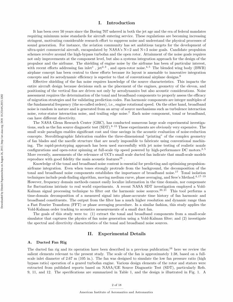
I. Introduction

It has been over 50 years since the Boeing 707 ushered in both the jet age and the era of federal mandatesrequiring minimum noise standards for aircraft entering service. These regulations are becoming increasingstringent, motivating considerable research effort to suppress noise and understand the physical processes ofsound generation. For instance, the aviation community has set ambitious targets for the development ofultra-quiet commercial aircraft, encapsulated by NASA’s N+2 and N+3 noise goals. Candidate propulsionschemes revolve around the high-bypass turbofan and the open rotor. Attainment of the noise goals requiresnot only improvements at the component level, but also a systems integration approach for the design of thepropulsor and the airframe. The shielding of engine noise by the airframe has been of particular interest,with recent efforts addressing fan inlet1 , jet2,3 , and open-rotor noise.4,5 The blended wing body (BWB)airplane concept has been central to these efforts because its layout is amenable to innovative integrationconcepts and its aerodynamic efficiency is superior to that of conventional airplane designs.6

Effective shielding of the fan noise requires knowledge of the source characteristics. This impacts theentire aircraft design because decisions such as the placement of the engines, geometry of the elevon, andpositioning of the vertical fins are driven not only by aerodynamics but also acoustic considerations. Noiseassessment requires the determination of the tonal and broadband components to properly assess the efficacyof migration strategies and for validating prediction codes. Fan harmonic components are integer multiples ofthe fundamental frequency (the so-called orders), i.e., engine rotational speed. On the other hand, broadbandnoise is random in nature and is generated from an array of source mechanisms such as turbulence interactionnoise, rotor-stator interaction noise, and trailing edge noise.7 Each noise component, tonal or broadband,can have different directivity.

The NASA Glenn Research Center (GRC), has conducted numerous large scale experimental investiga-tions, such as the fan source diagnostic test (SDT).8–15 These experiments are obviously very expensive. Thesmall scale paradigm enables significant cost and time savings in the acoustic evaluation of noise-reductionconcepts. Sterolithographic fabrication enables the three-dimensional “printing” of the complex geometryof fan blades and the nacelle structure that are nearly impossible to fabricate using conventional machin-ing. The rapid-prototyping approach has been used successfully with jet noise testing of realistic nozzleconfigurations and open-rotor spinning at full-scale tip speed powered by high-performance DC motors.2,5

More recently, assessments of the relevance of UCI’s small scale ducted fan indicate that small-scale modelsreproduce with good fidelity the main acoustic features16 .

Knowledge of the tonal and broadband noise content is essential for predicting and optimizing propulsion-airframe integration. Even when tones strongly protrude from the background, the decomposition of thetonal and broadband noise components establishes the importance of broadband noise.17 Tonal isolationtechniques include peak-finding algorithm, moving medium curve, phase averaging, and Sree’s Method.4,17–19

However, frequency domain methods cannot easily localize information in the time domain, nor compensatefor fluctuations intrinsic to real world experiments. A recent NASA SDT investigation employed a Vold-Kalman signal processing technique to filter out the harmonic noise sources.20,21 This tool performs atime-domain decomposition of a measured signal into phase-accurate time history of fan harmonic andbroadband constituents. The output from the filter has a much higher resolution and dynamic range thana Fast Fourier Transform (FFT) or phase averaging procedure. In a similar fashion, this study applies theVold-Kalman order tracking to acoustics measurements of a small duct fan.

The goals of this study were to: (1) extract the tonal and broadband components from a small-scalesimulator that captures the physics of fan noise generation using a Vold-Kalman filter; and (2) investigatethe spectral and directivity characteristics of the tonal and broadband noise sources.

II. Experimental Details

A. Ducted Fan Rig

The ducted fan rig and its operation have been described in a previous publication;16 here we review thesalient elements relevant to the present study. The scale of the fan is approximately 1:38, based on a full-scale inlet diameter of 2.67 m (105 in.). The fan was designed to simulate the low fan pressure ratio (highbypass ratio) operation of a geared turbofan engine. Various design elements of the rotor and stators wereextracted from published reports based on NASA/GE Source Diagnostic Test (SDT), particularly Refs.9, 11, and 12. The specifications are summarized in Table 1, and the design is illustrated in Fig. 1. A

2 of 18


Dow

nloa

ded

by D

imitr

i Pap

amos

chou

on

Aug

ust 2

6, 2

015

| http

://ar

c.ai

aa.o

rg |

DO

I: 1

0.25

14/6

.201

5-32

82

bell-mouth entry for the nacelle was chosen to prevent flow separation in the static test environment. Thenacelle (including the stators) and rotor were manufactured from plastic material using stereolithograpy.The nacelle features pressure ports for measuring the inlet static pressure and the outlet total pressure. Theaerodynamic performance was assessed by these pressure measurements.

Table 1. Ducted fan specifications

Parameter Specifications

Nacelle

Fan inlet diameter 70.0 mm

Fan exit diameter 71.0 mm

Nacelle exit to inlet area ratio 0.56

Design fan pressure ratio 1.15

Input power 5.0 kW (6.7 hp)

Rotor

Overall design Based on GE R4 fan

Count 14

Diameter 69.2 mm (0.4 mm tip clearance)

Design RPM 57000

Design Tip Mach 0.61

Hub-to-Tip ratio 0.42

Solidity 1.34 at pitch line

Blade Airfoil NACA 65-series

Blade Camber 56.6 ◦ (hub) to 6.2 ◦ (tip)

Blade Pitch Angle 51.6 ◦ (hub) to 28.3 ◦ (tip)

Blade Thickness/Chord Ratio 0.081 (hub) to 0.028 (tip)

Stator

Overall design Radial vane, based on low-count SDT configuration

Count 24

Solidity 2.21 (hub) to 1.04 (tip)

Blade Airfoil NACA 65-Series

Blade Camber 42.2 ◦ (hub) to 40.6 ◦ (tip)

Blade Thickness/Chord Ratio 0.0707 (hub) to 0.0698 (tip)

70-mm diameter

nacelle with bell

mouth inlet

14-blade rotor

24 stators

Neu Motors Model 1530-

1.5D brushless DC motor

Motor

cowling

Pylon

Scale factor = 38 (based on 104-inch fan diameter)

a) b)

Figure 1. Overview of the ducted fan design. a) Cross-sectional view; b) picture of the 3D printed rotor.

3 of 18


Dow

nloa

ded

by D

imitr

i Pap

amos

chou

on

Aug

ust 2

6, 2

015

| http

://ar

c.ai

aa.o

rg |

DO

I: 1

0.25

14/6

.201

5-32

82

The rotor was powered by a high-performance brushless DC motor (Neu Motors, Model 1530-1.5D) whichcan attain a surge power of 5.0 kW. The motor has an RPM/Volt (Kv) rating of 1350, meaning that it canspin at an RPM of 60,000 at the maximum rated voltage of 44 V. The motor was controlled using CastleCreations Phoenix 160 Amp electronic speed controller (ESC). Power to the speed controller was suppliedby two 6S (22.2 V ) lithium-ion polymer (Lipo) battery connected in series with a discharge rate of 30c anda capacity of 8300 mAh. The speed controller was controlled by a Spektrum AR6200 DSM2 six-channelreceiver connected wirelessly to a Spektrum DX7 2.4 GHz seven-channel radio. The receiver was poweredby a Castle Creations battery eliminator circuit (BEC PRO). The power components and their installationare depicted in Fig. 2.

Electronic Speed Controller (ESC) Castle Creations Phoenix 160-Amp

Arming

switch

Batteries 2 × 6S (22.2 V) Lipo

44.4 V total

Brushless DC motor Neu Model 1530-1.5D

1355 kV

60000 RPM max

2500 W continuous power

5000 W surge power

Six-Channel Receiver Spektrum AR6200 DSM2

2.4 GHz Seven-Channel Radio Spektrum DX7

Battery Eliminator Circuit (BEC) Castle Creations BEC Pro

Figure 2. Principal power components and their installation.

B. Test Facility

Acoustic measurements were conducted inside an anechoic chamber at UC Irvine’s Aeroacoustics Facility,depicted in Figs. 3 and 4. Twenty-three 3.2-mm condenser microphones (Bruel & Kjaer, Model 4138) witha frequency response of 140 kHz were used to survey the far-field acoustics. The microphones were arrangedtwelve on a downward arm (azimuth angle φ = 0◦) and eleven on a sideline arm (φ = 60◦). The polar angleθ is defined from the center of the fan exit plane relative to the downstream rotor axis, as shown in Fig. 3.Its approximate range was 15◦ to 110◦ for the downward arm, and 15◦ to 100◦ for the sideline arm. Theminimum microphone-to-nacelle distance was 0.8 m, or 11.4 fan diameters. This places the microphones inthe acoustic far field for the frequency range relevant to aircraft noise (i.e., higher than 50 Hz at full scale).

The microphones were connected, in groups of four, to six conditioning amplifiers (Bruel & Kjaer, Model2690-A-0S4). The 23 outputs of the amplifiers were sampled simultaneously, at 250 kHz per channel, bythree eight-channel multi-function data acquisition boards (National Instruments PCI-6143). A 24th outputchannel was assigned to the RPM sensor. National Instruments LabView software was used to acquire thesignals. The temperature and humidity inside the anechoic chamber were recorded to enable computationof the atmospheric absorption.

The sampling rate for each microphone was 250000 samples/second, and the number of samples for eachtest run was 262144 per microphone. The signals were re-sampled at constant angular increments of theshaft for computing the order tracking.22 The narrowband sound pressure level spectra were computedwith a 8192-point Fast Fourier Transform, giving a frequency resolution of 30.5 Hz. The SPL narrowband

4 of 18


Dow

nloa

ded

by D

imitr

i Pap

amos

chou

on

Aug

ust 2

6, 2

015

| http

://ar

c.ai

aa.o

rg |

DO

I: 1

0.25

14/6

.201

5-32

82

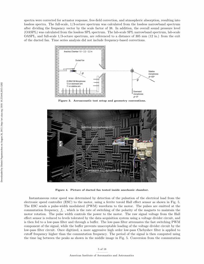
spectra were corrected for actuator response, free-field correction, and atmospheric absorption, resulting intolossless spectra. The full-scale, 1/3-octave spectrum was calculated from the lossless narrowband spectrumafter dividing the frequency vector by the scale factor of 38. In addition, the overall sound pressure level(OASPL) was calculated from the lossless SPL spectrum. The lab-scale SPL narrowband spectrum, lab-scaleOASPL, and full-scale 1/3-octave spectrum, are referenced to a distance of 305 mm (12 in.) from the exitof the ducted fan. Time series analysis did not include frequency-based corrections.

Anechoic Chamber 1.9 × 2.2 × 2.2 m

Ducted Fan

q

23 BK4138 Microphones

12 on downward arm

11 on sideline arm

f

Downward

microphones

f=0o

Sideline

microphones

f=60o

Figure 3. Aeroacoustic test setup and geometry conventions.

Sideline microphones (11)

Downward microphones (12)

Figure 4. Picture of ducted fan tested inside anechonic chamber.

Instantaneous rotor speed was determined by detection of the pulsation of the electrical load from theelectronic speed controller (ESC) to the motor, using a ferrite toroid Hall effect sensor as shown in Fig. 5.The ESC sends a pulse-width modulated (PWM) waveform to the motor. The pulses are emitted at thecommutation frequency, fc , which is the rate of switching of the polarity of the magnets to maintain themotor rotation. The pulse width controls the power to the motor. The raw signal voltage from the Halleffect sensor is reduced to levels tolerated by the data acquisition system using a voltage divider circuit, andis then fed to a low-pass filter and through a buffer. The low-pass filter attenuates the fast switching PWMcomponent of the signal, while the buffer prevents unacceptable loading of the voltage divider circuit by thelow-pass filter circuit. Once digitized, a more aggressive high order low-pass Chebyshev filter is applied tocutoff frequency higher than the commutation frequency. The period of the signal is then computed usingthe time lag between the peaks as shown in the middle image in Fig. 5. Conversion from the commutation

5 of 18


Dow

nloa

ded

by D

imitr

i Pap

amos

chou

on

Aug

ust 2

6, 2

015

| http

://ar

c.ai

aa.o

rg |

DO

I: 1

0.25

14/6

.201

5-32

82

period T to instantaneous frequency (BPF) is given by the formula f(t) = 2Nb/(TNp), where Np is thenumber of magnetic poles in the motor and Nb is the number of blades. The Neu 1530 motor has four poles,and the rotor has 14 blades. This method enabled the determination of a precise phase accurate frequencyfor each acoustic test run (the RPM signal was collected simultaneously with the microphone signals).

A representative time history of the motor frequency is plotted in Fig. 6. The low-pass filtered signal ofthe instantaneous frequency is depicted by the red line. It is observed that the shaft frequency fluctuates ata high frequency over a slowly varying RPM value that slows during the experiment. A key to the successfulimplementation of the Vold-Kalman filter is the precise knowledge of the structure to be tracked. The non-filtered (black) signal serves as a very accurate RPM input to the Vold-Kalman filter, such that the trackingfilter will follow the peaks of the tones (orders) instead of tracking the wrong frequency.

VOLTAGE

DIVIDER BUFFER

LOW-PASS

FILTER

DIGITAL

FILTER

Hall effect current sensor Wire from ESC to motor

CURRENT

MEASURE

PERIOD

𝟏

𝑻 ∗

𝟐 ∗ # 𝒃𝒍𝒂𝒅𝒆𝒔

# 𝒑𝒐𝒍𝒆𝒔

INSTANTANEOUS FREQUENCY

SIGNAL

(Sampled at

250 kS/s)

1000 1200 1400 1600 1800 2000-0.06

-0.04

-0.02

0

0.02

0.04

0.06

Time (ms)

Vo

lta

ge

(V)

1000 1200 1400 1600 1800 2000-0.06

-0.04

-0.02

0

0.02

0.04

0.06

Time (ms)

Vo

lta

ge

(V)

0 0.2 0.4 0.6 0.8 113.2

13.25

13.3

13.35

13.4

13.45

13.5

13.55

Time (s)

Fre

qu

ency

(k

Hz)

Figure 5. Flowchart of RPM measurement and phasor frequency determination process.

0 0.1 0.2 0.3 0.4 0.5 0.6 0.7 0.8 0.9 113.2

13.25

13.3

13.35

13.4

13.45

13.5

13.55

Time (sec)

Fre

qu

ency

(k

Hz)

Orginal signal

Low pass filtered

Figure 6. Frequency time trace during a typical test run (262144 samples). The red line represents the low-pass filtered component of the RPM sensor output. Rotor speed indicates an average RPM near 57,000 (13.33kHz). The rotor slows down slightly during the experiment.

III. Algorithum of the Vold-Kalman Filter

The Vold-Kalman filter, introduced by Vold and Leuridan,23 extracts the non-stationary periodic compo-nents from a signal using a known frequency vector (e.g., rotor RPM). Several additional works describe itsfunctionality and applications.21,24,25 The filter is formulated as a least-squares problem and can be solvedas a linear system. Similar to the Kalman filter, which is based on the process/ measurement equations (i.e.state-space model) and a global estimator (orthogonal projection)26 , the Vold-Kalman filter is based on the

6 of 18


Dow

nloa

ded

by D

imitr

i Pap

amos

chou

on

Aug

ust 2

6, 2

015

| http

://ar

c.ai

aa.o

rg |

DO

I: 1

0.25

14/6

.201

5-32

82

structural/data equations and a global estimator (least squares). Only the second-generation multi-orderVold-Kalman filter will be reviewed and applied in this paper.

A. Data Equation

Engineers are interested in signals that exhibit periodicity, i.e., events that occur repeatedly in time witha prescribed period.27 This may be a result of an oscillating spring/membrane, mechanical systems, orthe sound pressure generated by the periodic volume displacement of air by the blades of a propeller.These are deterministic processes. Broadband noise, in contrast, is typically generated by a more or lessstochastic process. Such noise sources include turbulence, vortex shedding, interaction effects, and representeverything that is uncorrelated with the RPM sensor signal. An arbitrary real-valued signal can be modeledas a summation of a deterministic periodic part consisting of K sine waves with varying phase and amplitude,plus a stochastic part of uncorrelated broadband noise η(t). This sinusoidal plus noise formulation is calledthe Wold decomposition.28 The total measured signal y(t) is of the form:

y(t) =

K∑k=1

xk(t) exp

(2πki

∫ t

0

f(t)dt

)+ η(t) (1)

Here the deterministic periodic signal is written in complex polar coordinates, with k indicating theorder extracted. The exponential term is called the complex phasor and represents a constant-amplitude,frequency-modulated carrier wave. The instantaneous frequency f(t) of the carrier wave is determined bythe tachometer or RPM sensor. The slowly time-varying (complex) amplitude xk(t) modulates the carrierwave (i.e. the complex phasor). The objective of the Vold-Kalman algorithm is to minimize the sum ofsquares of the errors (e.g., broadband signal) for a number of harmonics by properly choosing the complexenvelope xk(t). Storing the complex phasor on the diagonals of the matrix Ck, the above expression takesthe compact form:

y(t)−K∑k=1

Ckxk(t) = η(t) (2)

B. Structural Equation

The structural equation imposes smoothness on the complex envelope xk(t) by means of a backward finite-difference sequence. This is accomplished by minimizing the error ε(t) made in the smoothness of theenvelope, where the smoothness is represented by a low-order polynomial. The polynomial order designatesthe number of the filter poles. The equations for 1-,2-, and 3- pole filter coefficients are found by the Pascaltriangle:

∇xk[n] = xk[n]− xk[n− 1] = εk[n] (3a)

∇2xk[n] = xk[n]− 2xk[n− 1] + xk[n− 2] = εk[n] (3b)

∇3xk[n] = xk[n]− 3xk[n− 1] + 3xk[n− 2]− xk[n− 3] = εk[n] (3c)

Assuming a second-order difference, the system of structural equations with the complex envelope xk fororder k as the unknown takes the form of a matrix equation:

1 −2 1 0 · · ·0 1 −2 1 0 · · ·... 0 1 −2 1 0 · · ·

... 0. . .

. . .. . . 0 · · ·

1 −2 1 0

0 0 0 0 1 −2 1

xk[1]

xk[2]

xk[3]...

xk[n]

=

εk[3]

εk[4]

εk[5]...

εk[n]

(4)

Notice that the errors εk[1] and εk[2] cannot be determined since the stencil contains points outside thedomain of the complex envelope. For an order k, the matrix on the left hand side is a sparse band matrix

7 of 18


Dow

nloa

ded

by D

imitr

i Pap

amos

chou

on

Aug

ust 2

6, 2

015

| http

://ar

c.ai

aa.o

rg |

DO

I: 1

0.25

14/6

.201

5-32

82

(tridiagonal matrix in this example) with dimensions of (N − p)×N , p being the number of the filter poles(p = 2 in this example). In compact notation the matrix reads as:

Axk = εk (5)

C. The Least-Squares Problem

The set of data and structural equations creates an over-determined linear system for the desired waveformamplitude xk(t). No exact solution exists, nor does a two-sided inverse. A pseudo inverse can be obtainedusing ordinary least-squares, QR decomposition, or the singular value decomposition (SVD). Normally, theVold-Kalman filter uses least squares because of speed. Here, the objective is to estimate the non-randomcomplex envelope xk(t) by minimizing the square of the errors from the data and structural equations dueto non-periodic components and envelope roughness, respectively. Introducing a scalar weighing factor r, acost function is formulated to find the optimum solution in the sense of least squares:

J(x) =

K∑k=1

r2kεHk εk + ηHη (6)

The purpose of the weighting factor is to slant the prominence of the structural equation with that of thedata equation. For instance, if r is large the cost function is strongly influenced by the structural equationyielding a very smooth modulator. The value of r also determines the bandwidth of the filter. Large r resultsin very small bandwidth and vice-versa. The minimum is found by evaluating the derivative dJ/dxH = 0,and rearranging to a more familiar “normal” least-squares form:(

r2ATA+ I)xk = CHk y (7)

The equivalent “second-derivative” minimization requirement for a multidimensional problem is that thesymmetric hessian matrix (r2ATA + I) be positive definite. It can be shown that r2ATA + I is positivesemi-definite, and adding the identity matrix turns it positive definite. This property ensures that the matrixon the left hand side is invertible. Moreover, the matrix r2ATA+ I is independent of the tracked frequencyin Ck and the signal y. This allows for the matrix to be reused for tracking of orders with different phasors,reducing the extensive computational memory resource required. With regards to rotor noise separation, nocrossing orders exist. Efficient Vold-Kalman filtering is accomplished using multi-order tracking through asingle order scheme by simply changing the terms in the phasor term on the right hand side of Eq. 7 fordifferent harmonics, and solving the respective linear system independently. For instance, given the highsampling rate necessitated by small scale acoustical experiments, and the multiple orders tracked, the singleorder scheme drastically shrinks the matrix dimension from 1,750,000 to solving 7 decoupled matrices withdimension of 250,000. The expanded version of Eq. 7 for a two-pole Vold-Kalman filter and order k has theform:

r + 1 −2r r 0 · · ·−2r 5r + 1 −4r r 0 · · ·

... r −4r 6r + 1 −4r 0 · · ·

0 0 0. . .

. . .. . .

. . . · · ·

xk[1]

xk[2]

xk[3]...

xk[n]

=

CHk y[1]

CHk y[2]

CHk y[3]...

CHk y[n]

(8)

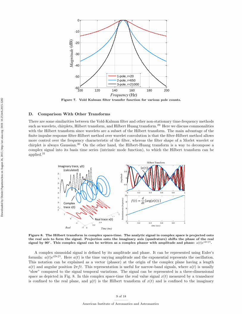
The linear system is very large, sparse, banded, and positive definite. This implies that the solution can beobtained efficiently by using Cholesky factorization. In the process of determining a solution the matrix onthe right hand side undergoes zero-phase low-pass filtering. The frequency response characteristic, definedby a -3 dB drop in magnitude, is controlled by the value of the weighting coefficient r. Fig. 7 depicts thebandwidth of the filter with varying pole counts and a weighting factor. A higher weighting factor resultsin a smaller bandwidth and a smoother varying amplitude as shown in the figure. However, the value of rshould not overshadow the effect of adding unity to the main diagonal. Typical Vold-Kalman order trackingcodes utilize a two-pole filter.

8 of 18


Dow

nloa

ded

by D

imitr

i Pap

amos

chou

on

Aug

ust 2

6, 2

015

| http

://ar

c.ai

aa.o

rg |

DO

I: 1

0.25

14/6

.201

5-32

82

100 120 140 160 180 200-60

-50

-40

-30

-20

-10

0

Frequency (Hz)

Ma

gn

itu

de

(dB

)

1-pole, r=20

2-pole, r=650

3-pole, r=21000

Figure 7. Vold Kalman filter transfer function for various pole counts.

D. Comparison With Other Transforms

There are some similarities between the Vold-Kalman filter and other non-stationary time-frequency methodssuch as wavelets, chirplets, Hilbert transform, and Hilbert Huang transform.29 Here we discuss commonalitieswith the Hilbert transform since wavelets are a subset of the Hilbert transform. The main advantage of thefinite impulse response filter-Hilbert method over wavelet convolution is that the filter-Hilbert method allowsmore control over the frequency characteristic of the filter, whereas the filter shape of a Morlet wavelet orchirplet is always Gaussian.30 On the other hand, the Hilbert-Huang transform is a way to decompose acomplex signal into its basis time series (intrinsic mode function), to which the Hilbert transform can beapplied.31

0

0.2

0.4

0.6

0.8

1

-2

-1

0

1

2

-2

-1.5

-1

-0.5

0

0.5

1

1.5

2

Time (ms)Real

Ima

gin

ary

0 0.2 0.4 0.6 0.8 1-1

-0.5

0

0.5

1

Am

plitu

de

Hilbert Transform

0 0.2 0.4 0.6 0.8 12

4

6

8

10

Inst

anta

neo

us

freq

uen

cy

time (sec)

Real trace x(t)

Imaginary trace, y(t) (calculated)

Complex trace z(t)

𝑧(𝑡)

𝑓 𝑡 =𝑑

𝑑𝑡arg(𝑧 𝑡 )

Figure 8. The Hilbert transform in complex space-time. The analytic signal in complex space is projected ontothe real axis to form the signal. Projection onto the imaginary axis (quadrature) shifts the phase of the realsignal by 90◦. This complex signal can be written as a complex phasor with amplitude and phase: a(t)ei2πft.

A complex sinusoidal signal is defined by its amplitude and phase. It can be represented using Euler’sformula: a(t)ei2πft. Here a(t) is the time varying amplitude and the exponential represents the oscillation.This notation can be explained as a vector (phasor) at the origin of the complex plane having a lengtha(t) and angular position 2πft. This representation is useful for narrow-band signals, where a(t) is usually“slow” compared to the signal temporal variations. The signal can be represented in a three-dimensionalspace as depicted in Fig. 8. In this complex space-time the real value signal x(t) measured by a transduceris confined to the real plane, and y(t) is the Hilbert transform of x(t) and is confined to the imaginary

9 of 18


Dow

nloa

ded

by D

imitr

i Pap

amos

chou

on

Aug

ust 2

6, 2

015

| http

://ar

c.ai

aa.o

rg |

DO

I: 1

0.25

14/6

.201

5-32

82

axis. When x(t) and y(t) are added vectorially, the result is a complex analytic trace z(t) = x(t) + iy(t),in the shape of a helical spiral extending along the time axis.32 Analytic means that the complex signalsatisfies the Cauchy-Riemann conditions, that is, the derivative of z(t) is path-independent and unique.The reason for converting the real signal into a complex trace is because the instantaneous amplitude andfrequency can be calculated by taking the magnitude and argument of z(t), as shown in the right image ofFig. 8. The real-valued signal of the Vold-Kalman filter is analogous to the filtered real-valued signal x(t)in the Hilbert transform.21 However, the phase of the signal is computed from the tachometer signal ratherthan computing the mapping on the imaginary plane. Since a phase-accurate estimate of the instantaneousfrequency is obtained directly from the tachometer, the complex phasor is already known. No unwrappingof the phase (revolute) and application of a Savitzky-Golay filter, or conjugate multiplication of adjacentcomplex samples (arg{z[n]z∗[n+1]}) are required to compute the instantaneous frequency.32 Thus, the Vold-Kalman filter only requires the linear estimation of the complex envelope Ck (analogous to |z(t)|) which isgenerated by the structural equation rather than the signal itself as in the Hilbert transform. Just like inwavelets, the Vold-Kalman filter is a subset of the more general Hilbert transform were information aboutthe signal phase is obtained a priori.

-2

-1

0

1

2

0

50

100

150

200

-2

-1.5

-1

-0.5

0

0.5

1

1.5

DisplacementTime (s)

Vel

oci

ty

0 50 100 150 2000

0.5

1

1.5

2

Time (s)

0 50 100 150 200-2

-1

0

1

2

Time (s)

Dis

pla

cem

ent

Hilbert

Vold Kalman

Figure 9. Oscillator system response in the (y,y,t) space, projecting the trajectory onto the displacement timeaxis gives the measured signal. Mapping the curve to space and velocity gives the phase portrait.

In Fig. 9, a representative solution for a forced linear oscillator described by the second-order nonau-tonomous differential equation y+2ζy+y = f cos(ωt) is graphed. y, t, ζ, f, and ω are the displacement, time,damping ratio, excitation amplitude, and excitation frequency, respectively. Projecting the trajectory ontothe displacement time axis gives the measured signal. Mapping the curve to space and velocity gives thephase portrait. White noise was added to the simulated solution. The stationary system is driven near theresonance frequency producing beats. Two times scales are present, an exponentially decaying envelope, andthe oscillation corresponding to the natural frequency of the system. The exponential decay is represented bythe trajectory inward spiral toward the origin. The linearity of the system implies a constant instantaneousfrequency, as illustrated in the right image of Fig. 9. The oscillations are periodic, deterministic, and aremodeled by a composition of a small number of monocomponent signals:

y(t) =

K∑k=1

xk(t) exp

(2πki

∫ t

0

f(t)dt

)(9)

Non-correlated signals are manifested in the broadband noise term, η(t). Here only one order exists,allowing effortless calculation of the complex envelope for both methods; if not, the results of the Hilberttransform are difficult to interpret when the data contain a range of frequencies and filtering or decompositionof the raw signal is required. To capture similar details to the Hilbert transform the Vold-Kalman bandwidthmust be tuned. There are several techniques for the estimation of the narrowband signal frequency bandwidthof the Hilbert transform. Nevertheless, when we examine the average variance of the frequency excursion of

10 of 18


Dow

nloa

ded

by D

imitr

i Pap

amos

chou

on

Aug

ust 2

6, 2

015

| http

://ar

c.ai

aa.o

rg |

DO

I: 1

0.25

14/6

.201

5-32

82

the signal around the mean value, the average spectrum bandwidth is:

σ2bw =

∫ ∞0

(ω − ω)2S(ω)dω = (ω2 − ω2) + A2 (10)

where ω, S(w), A are the angular frequency, power spectrum, and amplitude of the signal (A = |z(t)|).The overbars represent time averages. The equation was obtained from Parseval’s theorem and indicatesthat the average bandwidth is equal to the mean square value of the rate of the amplitude variation plusthe mean square value of the deviation from the baseband frequency.32,33 Using a frequency vector at thenatural frequency, the Vold-Kalman filter gives the envelope in red. Alternatively, the filter-Hilbert transformcomputed similar results as depicted in blue. As noted earlier for the Hilbert transform, the signal phasewas derived from the data rather than a tachometer.

Even though the real signal (red) is the same, the trajectory of the integral curve (Fig. 9) does notnecessarily match the analytic trace z(t) (Fig. 8), especially for non-linear systems. The addition of a non-linear cubic term y3 to the simple harmonic oscillator, leading to the Duffing oscillator, dramatically changesthe picture. Typically, the phase portrait becomes more distorted, generating sharp peaks and troughs inthe time series. Additionally, a Duffing oscillator exhibits time variations in its natural frequency.32,34 Inother words, the increased stiffness for large deflections is accompanied by a faster oscillation. Nevertheless,the filter also applies to the limit cycle response of non-linear systems. When the excitation frequencieschange, the responses will still be harmonics of the excitation for non-linear structures. Since mechanicalsystems normally have transfer characteristics dependent upon frequency, the amplitude and phase of thesesine waves will typically also change as the periodic loading change their speed.27 Table 2 compares theVold-Kalman filter with other noise separation techniques.

Table 2. Filter comparison

SpectralMethods

PhaseAveraging

HilbertTransform

Vold-Kalman

Sree’sMethod

Nonstationary No No Yes Yes Yes

Domain Frequency Time Time Time Frequency

Encoder No Yes No Yes No

Filter shape No No User set Adaptivebandpass

No

Phase accurate No No Yes Yes No

Processing speed Fastest Medium Medium Slowest Fast

IV. Acoustic Results

For all the conditions covered in this report, the RPM was 57200 ± 1.0 % as exemplified in Fig. 6. Thiscorresponds to a rotor tip Mach number of 0.61 ± 1.0 %. Fan exhaust total pressure was 2.2 psig, whichtranslates to FPR=1.15, rotor induced velocity of 87 m/s, fan exit velocity of 155 m/s, and power outputof 4400 W (5.9 hp). The calculated power output is consistent with the motor input power of 5 kW and aconversion efficiency of 88 %.

A two-pole second-generation, multi-order using single order scheme Vold-Kalman filter was used toisolate each harmonic from a narrow frequency band around the tracked tone while preserving accurate phaseinformation. To work out the phasor information in the data equation, the tracked tone was determinedby the instantaneous frequency of the rotor specified by the RPM sensor. Although the signal consists of arapidly changing frequency, the Vold-Kalman filter is able to track even at extreme slew rates. Filtering ofthe 23 microphone data for 7 orders took a few minutes on an Intel Xenon based desktop computer usingthe Matlab® backslash matrix solver. No down-sampling was applied. Even though extensive exploration ofacoustic assessment and shielding effects were investigated in our previous work,16 signal processing in thispaper involves only the isolated ducted fan. In addition, there was no acoustic distinction in the isolatedcase among the two azimuthal directions. Thus, the results are presented for only the downward azimuthaldirection. The acoustic results will be presented as follows:

11 of 18


Dow

nloa

ded

by D

imitr

i Pap

amos

chou

on

Aug

ust 2

6, 2

015

| http

://ar

c.ai

aa.o

rg |

DO

I: 1

0.25

14/6

.201

5-32

82

(a) Time history, plotted for various polar angles, referenced to 305-mm arc.

(b) Narrowband SPL spectra in laboratory scale, referenced to 305-mm arc.

(c) Overall Sound Pressure level (OASPL) in laboratory scale, referenced to 305-mm arc.

(d) Directivity of selected 1/3-octave band levels (full-scale), referenced to 305-mm arc.

(e) Comparison with NASA large scale test, UCI data referenced to a linear traverse displaced 305 mm fromthe model centerline.

The standard color representation followed throughout this paper is:

• Total measured acoustic signal - Red

• Broadband (difference between raw and BPF Harmonics) - Blue

• BPF Extracted Harmonics (sum of all individual orders) - Black

A. Decomposition of Time Traces

We first examine the Vold-Kalman decomposition of microphone signals at various polar angles. The resultsare plotted in Fig. 10. The amplitudes of the noise components are dependent on the polar emission angle.At a polar angle of θ = 69.4◦ the amplitude of the overall pressure fluctuation is largest. At polar anglesclose to the downstream axis, the amplitude of the broadband noise encompasses the majority of the signal.On the other hand, the magnitude of the tonal noise is greatest at θ=69.4◦. To properly assess the relativeimportance of the broadband noise or harmonics, the energy of each waveform must be integrated over afinite octave band interval as done in Section IV.C.

0 0.2 0.4 0.6 0.8 1-60

-40

-20

0

20

40

60

Pre

ssu

re (

Pa)

= 20.7 = 0.0

0 0.2 0.4 0.6 0.8 1-60

-40

-20

0

20

40

60

Pre

ssu

re (

Pa)

Time (sec)

= 43.4 = 0.0

0 0.2 0.4 0.6 0.8 1-60

-40

-20

0

20

40

60

Pre

ssu

re (

Pa)

= 69.4 = 0.0

0 0.2 0.4 0.6 0.8 1-60

-40

-20

0

20

40

60

Pre

ssu

re (

Pa)

Time (sec)

= 99.2 = 0.0

Figure 10. Time domain signal decomposition of the ducted fan noise at various polar angles. Total signal(red), broadband (blue), harmonic (black).

B. Narrowband Spectra

The second set of assessments consists of conventional spectral analysis of the Vold-Kalman filtered signalsfor two polar angles, θ=20.7◦ and 99.2◦. The SPL narrowband spectra were corrected for actuator response,free-field correction, and atmospheric absorption, resulting into lossless spectra. Narrowband spectra areshown in Fig. 11. Spectral analysis of the microphone signal shows that tones up to 7× BPF were resolved.Hence, seven orders were filtered from the total signal using the Vold-Kalman filter. The Vold-Kalmanweighting factor was determined by minimizing the “divots” (or negative peaks) in the broadband spectrum,

12 of 18


Dow

nloa

ded

by D

imitr

i Pap

amos

chou

on

Aug

ust 2

6, 2

015

| http

://ar

c.ai

aa.o

rg |

DO

I: 1

0.25

14/6

.201

5-32

82

giving a bandwidth of 1 Hz. The weighting factor was below the recommended limit described by Tuma fora two-pole, second-generation filter.24 The black line (middle image) represents the harmonic componentsthat were isolated from the total signal. The bandwidth of each tone relates to the tonal energy removed atthat particular order. The sum of the extracted tonal signal forms the BPF harmonic signal. Subtractionof the total signal from the BPF harmonics (black) yields the broadband component (blue). Comparing thespectra at the two polar angles, the harmonic content is more prevalent near the rotational plane (θ ∼ 90◦).

20 40 60 80 100

40

60

80

SP

L (d

B/H

z)

θ = 20.7ο φ = 0.0ο

Total

20 40 60 80 100

40

60

80

SP

L (d

B/H

z)

θ = 99.2ο φ = 0.0ο

20 40 60 80 100

40

60

80

SP

L (d

B/H

z) Harmonic

20 40 60 80 100

40

60

80

SP

L (d

B/H

z)

20 40 60 80 100

40

60

80

SP

L (d

B/H

z)

Frequency (kHz)

Broadband

20 40 60 80 100

40

60

80

SP

L (d

B/H

z)

Frequency (kHz)Figure 11. Narrowband SPL spectra at two polar angles. Total signal (top), harmonic (middle), broadband(bottom).

(degrees)

Fre

quen

cy (

KH

z)

Measured Signal

20 40 60 80 1000

10

20

30

40

50

60

70

80

90

100

(degrees)

Harmonic

20 40 60 80 1000

10

20

30

40

50

60

70

80

90

100

(degrees)

Broadband

20 40 60 80 1000

10

20

30

40

50

60

70

80

90

100

SP

L (

dB

/Hz)

30

35

40

45

50

55

60

65

70

75

80

Figure 12. Countour plots of narrowband SPL spectra.

Fig. 12 displays contour maps of the SPL versus frequency and polar angle for the total and decomposedsignals. As evident in the contour maps of the harmonic component, rotor harmonics ranging from 1×BPFthrough 7×BPF are extracted. The tonal energy of the filtered (broadband) signal is substantially reducedcompared to the measured signal. The broadband signal still retains small remnants of tonal noise, which

13 of 18


Dow

nloa

ded

by D

imitr

i Pap

amos

chou

on

Aug

ust 2

6, 2

015

| http

://ar

c.ai

aa.o

rg |

DO

I: 1

0.25

14/6

.201

5-32

82

is the effect of some broadband noise being weakly correlated with the shaft orders. The subtraction oftonal noise makes a more pronounced impact at low frequency, indicating the relative strength of the tonalcomponent there. Figure 12 also serves to illustrate the directivity of sound versus frequency, with a peakevident near θ = 60◦.

C. Directivity of 1/3-Octave Spectra

Although the narrowband spectra provide a complete representation of the frequency content of the signal,engineering applications often rely on the 1/3-octave spectra. Furthermore, the 1/3 octave spectra allowfor the proper assessment of the energy distribution in the harmonic and broadband components.35 This isessentially a smoothing technique which integrates noise over frequency ranges whose widths are proportionalto their center frequencies. The 1/3-octave band spectrum was calculated from the scaled-up, lossless narrow-band spectrum by integrating the energy content in each frequency band. We examine the directivity of thefollowing bands, and indicate in parentheses the contained tones: band 9 (1×BPF), band 12 (2×BPF), band14 (3×BPF), and band 16 (4×BPF and 5×BPF). The directivities of those bands are plotted in Fig. 13.There are significant differences in the direction of peak emission for the various bands, band 9 peaking nearθ = 80◦ (i.e., close to the plane of rotation), whereas the higher bands peak near θ = 50◦. The directivitiesof the harmonic and broadband components tend to be similar, except for some oscillations in the harmoniccontent of band 14. It is evident that the energies of the tonal and broadband contents are similar for thelower bands, while the broadband content dominates the higher bands.

20 40 60 80 10085

90

95

100

105

SP

L (

dB

)

20 40 60 80 10050

60

70

80

90

100

110

SP

L (

dB

)

(deg)

20 40 60 80 10050

60

70

80

90

100

110

SP

L (

dB

)

20 40 60 80 10050

60

70

80

90

100

110

SP

L (

dB

)

(deg)

Band 09320 HzContains 1*BPF



Band 161612 Hz

4 & 5*BPF




Band 161612 Hz

4 & 5*BPF




Band 161612 Hz

4 & 5*BPF

Figure 13. One-third octave band directivities for four bands. Full-scale frequencies are shown. Total signal(red), broadband (blue), harmonic (black).

D. Overall Sound Pressure Level

Integrated noise metrics such as the overall sound pressure level (OASPL) describe the total energy containedin the spectrum. The OASPL was calculated by integrating the lossless SPL spectrum over all resolvedfrequencies. Fig. 14 plots the OASPL versus polar angle for the total, harmonic, and broadband signals. Forthe total and broadband component the energy peaks near θ = 60◦. The tonal component has a double peakat θ = 40◦ and 80◦, an its level is at least 5 dB below the broadband level. The tonal component shows asharp drop-off with polar angle away from the range of peak emission.

14 of 18


Dow

nloa

ded

by D

imitr

i Pap

amos

chou

on

Aug

ust 2

6, 2

015

| http

://ar

c.ai

aa.o

rg |

DO

I: 1

0.25

14/6

.201

5-32

82

0 20 40 60 80 100 12090

95

100

105

110

115

OA

SP

L (

dB

)

(deg)

OASPL directivity

Figure 14. OASPL directivity for the noise components. Total signal (red), broadband (blue), harmonic(black).

E. Comparison with NASA Large Scale Tests

In this section we make qualitative comparisons of our results with large-scale fan acoustic data acquiredat NASA Langley’s 9’× 15’ tunnel using a continuously traversing microphone.20,21 There are significantdifferences in the fan design and operating conditions between the UCI and NASA rigs. A quantitativecomparison in thus impossible. However, the NASA experiment being the only known fan test where asignal decomposition was carried out, we are compelled to try a qualitative comparison.

Table 3. Summary of fan specifications and experimental conditions

Quantity UCI NASA

Scale 1:38 1:5

Diameter 2.67 in 22 in

Mtunnel 0 0.1

Mtip 0.61 1.08

Rotor count 14 22

Stator count 24 26

FPR 1.15 1.47

Power 6.7 hp 5000 hp

Fan hub/ tip ratio 0.42 0.30

Scan Method Fixed array Continuous scan

Polar angle 15◦ to 110◦ 46◦ to 152◦

Table 3 summarizes the sizes, operating conditions, and measurement approaches of the two experiments.The most important operational difference was that the NASA rotor was transonic, while the UCI rotor wassubsonic. Consequently, the NASA rotor emitted multiple pure tones (MPTs), in addition to the conventionaltonal and broadband noise. MPTs are caused by the formation of leading-edge shocks on the suction sideof the blades.36 The resulting nonlinear quadrupole term transfers acoustical energy from BPF harmonicsto other modes that radiate upstream.37 For a perfect fan, with meticulous blade spacing and uniformblade geometry, the shock system will only emit energy at integer multiple of the BPF. However, naturalmanufacturing variations produce shocks of non-uniform amplitude and spacing, resulting in numerous tonesin addition to the BPF harmonics. These additional harmonics are called MPTs and are often referred to as“buzz saw” noise. Some MPT harmonics can be louder than the BPF tones. Buzz saw tones are deterministicand are separated as a harmonic component.

15 of 18


Dow

nloa

ded

by D

imitr

i Pap

amos

chou

on

Aug

ust 2

6, 2

015

| http

://ar

c.ai

aa.o

rg |

DO

I: 1

0.25

14/6

.201

5-32

82

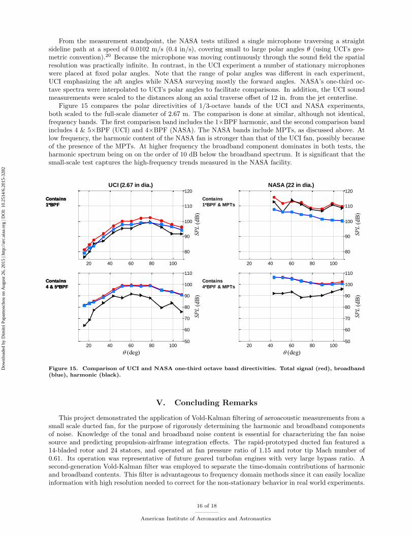
From the measurement standpoint, the NASA tests utilized a single microphone traversing a straightsideline path at a speed of 0.0102 m/s (0.4 in/s), covering small to large polar angles θ (using UCI’s geo-metric convention).20 Because the microphone was moving continuously through the sound field the spatialresolution was practically infinite. In contrast, in the UCI experiment a number of stationary microphoneswere placed at fixed polar angles. Note that the range of polar angles was different in each experiment,UCI emphasizing the aft angles while NASA surveying mostly the forward angles. NASA’s one-third oc-tave spectra were interpolated to UCI’s polar angles to facilitate comparisons. In addition, the UCI soundmeasurements were scaled to the distances along an axial traverse offset of 12 in. from the jet centerline.

Figure 15 compares the polar directivities of 1/3-octave bands of the UCI and NASA experiments,both scaled to the full-scale diameter of 2.67 m. The comparison is done at similar, although not identical,frequency bands. The first comparison band includes the 1×BPF harmonic, and the second comparison bandincludes 4 & 5×BPF (UCI) and 4×BPF (NASA). The NASA bands include MPTs, as discussed above. Atlow frequency, the harmonic content of the NASA fan is stronger than that of the UCI fan, possibly becauseof the presence of the MPTs. At higher frequency the broadband component dominates in both tests, theharmonic spectrum being on on the order of 10 dB below the broadband spectrum. It is significant that thesmall-scale test captures the high-frequency trends measured in the NASA facility.

20 40 60 80 100

80

90

100

110

120

SP

L (

dB

)

UCI (2.67 in dia.)

20 40 60 80 10050

60

70

80

90

100

110

SP

L (

dB

)

(deg)

20 40 60 80 100

80

90

100

110

120

NASA (22 in dia.)

SP

L (

dB

)

20 40 60 80 10050

60

70

80

90

100

110

(deg) S

PL

(d

B)

Contains

1*BPF

Contains

4 & 5*BPF

Contains

1*BPF

Contains

4 & 5*BPF

Contains

1*BPF

Contains

4 & 5*BPF

Contains

1*BPF & MPTs

Contains

4*BPF & MPTs

Figure 15. Comparison of UCI and NASA one-third octave band directivities. Total signal (red), broadband(blue), harmonic (black).

V. Concluding Remarks

This project demonstrated the application of Vold-Kalman filtering of aeroacoustic measurements from asmall scale ducted fan, for the purpose of rigorously determining the harmonic and broadband componentsof noise. Knowledge of the tonal and broadband noise content is essential for characterizing the fan noisesource and predicting propulsion-airframe integration effects. The rapid-prototyped ducted fan featured a14-bladed rotor and 24 stators, and operated at fan pressure ratio of 1.15 and rotor tip Mach number of0.61. Its operation was representative of future geared turbofan engines with very large bypass ratio. Asecond-generation Vold-Kalman filter was employed to separate the time-domain contributions of harmonicand broadband contents. This filter is advantageous to frequency domain methods since it can easily localizeinformation with high resolution needed to correct for the non-stationary behavior in real world experiments.

16 of 18


Dow

nloa

ded

by D

imitr

i Pap

amos

chou

on

Aug

ust 2

6, 2

015

| http

://ar

c.ai

aa.o

rg |

DO

I: 1

0.25

14/6

.201

5-32

82

The results shows that the energies of the tonal and broadband contents are similar for the lower frequencybands, while the broadband component dominates the higher frequency bands. Corresponding trends inenergy distribution between the components were found in large-scale NASA experiments. There are distinctdifferences in the polar directivities of the harmonic and broadband noise. The Vold-Kalman filter has proveneffective and useful for separating the noise components. The ultimate importance of harmonic-versusbroadband noise will be determined by the perceived noise level metric, which includes tone corrections.This was outside the scope of the present paper but will be the topic of future studies.

Complementing our earlier studies of the isolated and installed small-scale ducted fan,16 this work demon-strates that important aspects of fan noise can be studied at low cost in university-scale facilities, leveragingadvances in additive manufacturing and brushless motor technology. Innovative processing methods such asthe Vold-Kalman filter can be applied not only to the signals of the individual microphones but also to time-series-based acoustic imaging. The combination of inexpensive test rigs with advanced measurement andprocessing methods (such as the continuous-scan technique used at NASA) holds promise for fundamentalgains in our knowledge of the fan noise source and for constructing models for fan noise and its interactionswith the airframe.

AcknowledgmentWe thank Dr. Havard Vold of ATA Engineering, Inc., for his advice and guidance on the formulation of

the Vold Kalman filter for our experiment, and for enabling comparisons with his code.

References

1Gerhold, C., Clark, L., and Dunn, M., “Investigation of Acoustic Shielding by Wedge-Shaped Airframe,” Journal of theSound and Vibration, Vol. 294, No. 1-2, 2006, pp. 49–63.

2Mayoral, S. and Papamoschou, D., “Effects of Source Redistribution on Jet Noise Shielding,” AIAA 2010-0652, Jan. 2010.3Thomas, R. and Burley, C., “Hybrid Wing Body Aircraft System Noise Assesment with Propulsion Airframe Aeroacoustic

Experiments,” AIAA 2010-3913, 2010.4Berton, J., “Empennage Noise Shielding Benefits for an Open Rotor Transport,” AIAA 2011-2764, June 2011.5Truong, A. and Papamoschou, D., “Aeroacoustic Testing of Open Rotors at Very Small Scale,” AIAA 2013-0217, Jan.

2013.6Liebeck, R., “Design of the Blended Wing Body Subsonic Transport,” Journal of Aircraft , Vol. 41, No. 1, 2004, pp. 10–25.7Magliozzi, B., Hanson, D., and Amiet, R., “Propeller and Profan Noise,” Tech. Rep. N92-10598 01-71, NASA Langley

Research Center, Hampton, VA, July 1991.8Topol, A., Ingram, C., Larkin, M., Roche, C., and Thulin, R., “Advanced Subsonic Technonolgy (AST) 22-Inch Low

Noise Research Fan Rig Preliminary Design of ADP-Type Fan 3,” Tech. Rep. NASA/CR-2004-212718, NASA Langley ResearchCenter, Hampton, VA, Feb 2004.

9Hughes, C., Jeracki, R., Woodward, R., and Miller, C., “Fan Noise Source Diagnoistic Test-Rotor Alone AerodynamicsPerformance Results,” NASA/TM-2005-211681 (AIAA-2002-2426), April 2005.

10Heidelberg, L., “Fan Noise Source Diagnostic Test - Tone Model Structure Results,” NASA/TM-2002-211594 (AIAA-2002-2428), April 2002.

11Morin, B., “Broadband Fan Noise Prediction System for Turbofan Engines, Volume 1: Setup BFANS User’s Manual andDeveloper’s Guide,” Tech. Rep. CR-2010-216898, NASA, Nov 2010.

12Morin, B., “Broadband Fan Noise Prediction System for Turbofan Engines, Volume 3: Validation and Test Cases,” Tech.Rep. CR-2010-216898, NASA, Nov 2010.

13Hughes, C., Jeracki, R., Woodward, R., and Miller, C., “Aerodynamic Performance of Scale-Model Turbofan OutletGuide Vanes Designed for Low Noise,” NASA/TM-2001-211352 (AIAA-2002-0374), Dec. 2001.

14Woodward, R., “Comparison of Far-Field Noise for Three Significantly Different Model Turbofans,” AIAA Paper 2008-0049 , Jan 2008.

15Woodward, R., Elliott, D., Higher, C., and Berton, J., “Benefits of Swept-and-Leaned Stators for Fan Noise Reduction,”AIAA Journal , Vol. 38, No. 6, 2001.

16Truong, A. and Papamoschou, D., “Experimental Simulation of Ducted Fan Acoustics at Very Small Scale,” AIAA2014-0718, Jan. 2014.

17Parry, A.B., K. M. and Tester, B., “Relative importance of open rotor tone and broadband noise sources,” AIAA 2011-2763, June 2011.

18Stephens, D. and Envia, E., “Acoustic Shielding for a Model Scale Counter-Rotation Open Rotor,” NASA/TM-2012-217227 (AIAA-2011-2940), Jan. 2012.

19Sree, D. and Stephens, D., “Tone and Broadband Noise Separation from Acoustic Data of a Scale-Model Counter-RotatingOpen Rotor,” AIAA 2014-2744, June 2014.

20Shah, P., Vold, H., Hensley, D., E., E., and D., S., “A High-Resolution, Continuous-Scan Acoustic Measurement Methodfor Turbofan Engine Applications,” ASME Paper GT2014-27108, June 2014.

17 of 18


Dow

nloa

ded

by D

imitr

i Pap

amos

chou

on

Aug

ust 2

6, 2

015

| http

://ar

c.ai

aa.o

rg |

DO

I: 1

0.25

14/6

.201

5-32

82

21Stephens, D. and Vold, H., “Order Tracking Signal Processing for Open Rotor Acoustics,” Journal of Sound and Vibra-tion, Vol. 333, No. 16, 2014, pp. 3818–830.

22Fyfe, K. and Munck, D., “Analysis of Computed Order Tracking,” Mechanical Systems and Signal Processing, Vol. 11,No. 2, 1997, pp. 187–205.

23Vold, H. and Leuridan, J., “High Resolution Order Tracking at Extreme Slew Rates Using Kalman Tracking Filters,”SAE Technical Paper 931288, May 1993.

24Tuma, J., “Setting the Passband Width in the Vold-Kalman Tracking Filter,” 12th International Congress on Sound andVibration, 2005.

25Feldbauer, C. and Holdrich, R., “Realization of a Vold-Kalman Tracking Filter- A Least Squares Problem,” Proceedingsof the COST-6 Conference on Digital Audio Effects (DAFX-00), Dec. 2000.

26Kalman, R., “A New Approach to Linear Filtering and Prediction Problems,” Journal of Basic Engineering, Transactionsof ASME , Vol. 82, 1960, pp. 35–45.

27Herlufsen, H., Gade, S., Hansen, K., and Vold, H., “Characteristics of the Vold-Kalman Order Tracking Filter,” Brueland Kjaer Technical Review, April 1999.

28Wold, H., A Study in the Analysis of Stationary Time Series, Ph.D. thesis, Stockhom University, 1938.29Huang, N., Wu, M., Qu, W., Long, S., and Shen, S., “Applications of Hilbert-Huang transform to non-stationary financial

time series analysis,” May 2009, pp. 245–268.30Cohen, M., Analyzing Neural Time Series Data, The MIT Press, Cambridge.31Oweis, R. and Abdulhay, E., “Seizure Classification in EEG Signals Utilizing Hilbert-Huang Trasnform,” Biomedical

Engineering Online, May 2011, pp. 10–38.32Feldman, M., “Hilbert Transform In Vibration Analysis,” Mechanical Systems and Signal Processing, Vol. 25, No. 3,

April 2011, pp. 735–802.33Cohen, L. and Lee, C., “Standard Deviation Of Instantaneous Frequency,” Acoustic, Speech, and Signal Processing,

Vol. 4, 1989, pp. 2238–2241.34Kovacic, I. and Brennan, M., The Duffing Equation: Nonlinear Oscillators and their Behavior , John Wiley and Sons,

New Jersey, 1st ed., 2011.35Vold, H., “Sine Waves Are Stubborn Things,” Sound and Vibrations, June 2013.36Goldstein, A., Glaser, F., and Coats, J., “Acoustic Properties of a Supersonic Fan,” NASA/TN-1973-15025, Jan. 1973.37Han, F., Shieh, C., Sharma, A., and Paliath, U., “Multiple Pure Tone Noise Prediction and Comparison with Static

Engine Test Measurement,” AIAA 2007-3523, May 2007.

18 of 18


Dow

nloa

ded

by D

imitr

i Pap

amos

chou

on

Aug

ust 2

6, 2

015

| http

://ar

c.ai

aa.o

rg |

DO

I: 1

0.25

14/6

.201

5-32

82

harmonic and broadband separation of noise from a small

Documents