harmonic embeddings for linear shape analysis - uclavision.ucla.edu/papers/duciysr06.pdf ·...
TRANSCRIPT
J Math Imaging Vis 25: 341–352, 2006c© 2006 Springer Science + Business Media, LLC. Manufactured in The Netherlands.
DOI: 10.1007/s10851-006-7249-8
Harmonic Embeddings for Linear Shape Analysis
ALESSANDRO DUCIComputer Science Department, University of California at Los Angeles, Los Angeles - CA 90095
ANTHONY YEZZIElectrical and Computer Engineering, Georgia Institute of Technology, Atlanta - 30332
STEFANO SOATTOComputer Science Department, University of California at Los Angeles, Los Angeles - CA 90095
KELVIN ROCHAElectrical and Computer Engineering, Georgia Institute of Technology, Atlanta - 30332
Published online: 9 October 2006
Abstract. We present a novel representation of shape for closed contours in R2 or for compact surfaces in R3
explicitly designed to possess a linear structure. This greatly simplifies linear operations such as averaging, principalcomponent analysis or differentiation in the space of shapes when compared to more common embedding choicessuch as the signed distance representation linked to the nonlinear Eikonal equation. The specific choice of implicitlinear representation explored in this article is the class of harmonic functions over an annulus containing thecontour. The idea is to represent the contour as closely as possible by the zero level set of a harmonic function,thereby linking our representation to the linear Laplace equation. We note that this is a local represenation withinthe space of closed curves as such harmonic functions can generally be defined only over a neighborhood of theembedded curve. We also make no claim that this is the only choice or even the optimal choice within the classof possible linear implicit representations. Instead, our intent is to show how linear analysis of shape is greatlysimplified (and sensible) when such a linear representation is employed in hopes to inspire new ideas and additionalresearch into this type of linear implicit representations for curves. We conclude by showing an application forwhich our particular choice of harmonic representation is ideally suited.
1. Introduction
The analysis and representation of shape is at thebasis of many visual perception tasks, from classifi-cation and recognition to visual servoing. This is a vastand complex problem, which we have no intention of
addressing in its full generality here. Instead, we con-centrate on a specific issue that relates to the represen-tation of closed, planar contours or compact surfacesin 3D space. Even this issue has received considerableattention in the literature. In particular, in their workon statistical shape influence in segmentation [20],
342 Duci et al.
Leventon et al. have proposed representing a closedplanar contour as the zero level set of a function inorder to perform linear operations such as averag-ing or principal component analysis. The contour isrepresented by the embedding function, and all op-erations are then performed on the embedded repre-sentation. They choose as their embedding functionthe signed distance from the contour (whose differen-tial structure is described by the non-linear EikonalEquation) and implement its evolution in the numer-ical framework of level sets pioneered by Osher andSethian [27].
While this general program has proven effectivein various applications, the particular choice of em-bedding function presents several difficulties, becausesigned distance functions are not a closed set underlinear operations: the sum or difference of two signeddistance functions is not a signed distance function(an immediate consequence of their nonlinear differ-ential structures). Consequently, the space cannot beendowed with a probabilistic structure in a straight-forward manner, and repeated linear operations, in-cluding increments and differentiation, eventually leadto computational difficulties that are not easily ad-dressed within this representation. Alternative meth-ods that possess a linear structure rely on parametricrepresentations. For instance various forms of splines[6, 7], cannot guarantee that topology (or even theembeddedness) of the shape is preserved under sig-nificant variations of the control points. Furthermore,such representations are not geometric as they dependupon an arbitrary choice of parameterization for thecontour. Geometricized parametric representations uti-lizing the arclength parameter suffer from the samenonlinearity problem as implicit representations uti-lizing the signed distance to the curve. While it ispossible to generalize the notions of mean shapes andPCA to nonlinear representations, especially when theycan be endowed with a Riemannian structure, (seefor example [17]), it is decidely more complicatedand often involves rather expensive computationalalgorithms.
In this paper, we present a novel implicit represen-tation of shape for closed planar contours and compactsurfaces in R3 that is geometric and explicitly designedto possess a (locally) linear structure. This allows lin-ear operations such as principal component analysis ordifferentiation to be naturally defined and easily car-ried out. The basic idea consists of, again, representingthe contour or surface as the zero level set of a function,
but this time the function belongs to a linear (or quasi-linear1) space. While previous methods relied on the(non-linear) Eikonal equation, ours relies on Laplaceequation, which is linear. Our representation allows ex-ploring the neighborhood of a given shape while guar-anteeing that the topology and the embeddedness of theoriginal shape is preserved, even under large variationsof the parameters in our representation (the boundaryvalues of the harmonic function).
We should point out that the primary goal here isto show through an example how a linear implicit rep-resentation of contours or surfaces can simplify (andjustify) linear operations such as averaging and prin-ciple component analysis. It is not our claim that theuse of Laplace’s equation is the optimal choice. It is,however, a well studied PDE whose known propertiesallow us to conclude various analytical and topologicalproperties of the curves we seek to represent. Furthersome recent attention to shape analysis via Rieman-nain structures based on nonlinear representations ofcurves using harmonic functions is presented in [29](The authors wonder, in fact, if the linear representa-tion presented here may be tied to of local linearizationof this representation in the neighborhood of a givenshape). We also show in Section 5 an application that isideally suited for our particular choice of harmonic em-bedding. Beyond these considerations, however, mostof what we are illustrating in this work could carrythrough for other classes of linear or quasilinear em-bedding functions.
We introduce the simplest form of harmonic embed-ding in Section 2, where we point out some of its diffi-culties. We then extend the representation to a relatedanisotropic operator in Section 3, and discuss its finite-dimensional implementation in Section 4. In Section 5we show an application to measuring tissue thicknesson segmented medical image data. Finally, we illustratesome of the properties of this representation in Section6. While the detailed discussion is restricted to the 2Dcase, the extension to 3D is straight-forward and obvi-ous. We therefore will make not repeat the same detailsin 3D, but we will however show 3D examples in theresults section.
1.1. Relation to Previous Work
The literature on shape modeling and representation istoo vast to review in the limited scope of this paper.It spans at least a hundred years of research in dif-ferent communities from mathematical morphology
Harmonic Embeddings for Linear Shape Analysis 343
to statistics, geology, neuroanatomy, paleontology, as-tronomy etc. Some of the earlier attempts to formalizea notion of shape include D’Arcy Thompson’s treatise“Growth and Form” [32], the work of Matheron on“Stochastic Sets” [24] as well as that of Thom, Gib-lin and others [ 8, 31]. The most common represen-tations of shape rely on a finite collection of points,possibly defined up to equivalence classes of group ac-tions [5, 13, 19, 23]. These tools have proven usefulin contexts where distinct “landmarks” are available,for instance in comparing biological shapes with dis-tinct “parts.” However, comparing objects that have adifferent number of parts, or objects that do not haveany distinct landmark, is elusive under the aegis of sta-tistical shape spaces. Koenderink [18] is credited withproviding some of the key ideas involved in formalizinga notion of shape that matches our intuition. However,Mumford has critiqued current theories of shape on thegrounds that they fail to capture the essential featuresof perception [26].
“Deformable Templates,” pioneered by Grenander[11], do not rely on “features” or “landmarks;” rather,images are directly deformed by a (possibly infinite-dimensional) group action and compared for the bestmatch in an “image-based” approach [38]. Another lineof work uses variational methods and the solution ofpartial differential equations (PDEs) to model shapeand to compute distances and similarity. In this frame-work, not only can the notion of alignment or distancebe made precise [3, 15, 25, 28, 37], but quite sophis-ticated theories that encompass perceptually relevantaspects can be formalized in terms of the properties ofthe evolution of PDEs (e.g. [16]). The work of Kimiaet al. [14] describes a scale-space that corresponds tovarious stages of evolution of a diffusing PDE, and a“reacting” PDE that splits “salient parts” of planar con-tours by generating singularities. [14] also contains anice taxonomy of existing work on shape and defor-mation and a review of the state of the art as of 1994.
The variational framework has also proven very ef-fective in the analysis of medical images [21, 22, 33,36]. Although most of the ideas are developed in adeterministic setting, many can be transposed to aprobabilistic context Scale-space is a very active re-search area, and some of the key contributions asthey relate to the material of this paper can be foundin [1, 2, 12, 30] and references therein. Leventon etal. [20] perform principal component analysis in thealigned frames to regularize the segmentation of re-gions with low contrast in brain images. Similarly, [35]
performs the joint segmentation of a number of imagesby assuming that their registration (stereo calibration)is given.
We present a novel representation of shape that sup-ports linear operations. We only consider closed planarcontours, and even within this set our representationcannot capture any shape; it does not include a notionof hierarchy or compositionality, which are crucial ina complete theory of shape. Despite its limitations thatrestrict the class of shapes and the analysis to theirglobal properties, our representation has desirable fea-tures when it comes to linear analysis. In fact, it allowsus to naturally take linear combinations of shapes; per-forming principal component analysis (PCA) on theembedding function results in a natural notion of defor-mation on the underlying shapes. Endowing the spacewith a probabilistic structure, although not addressedin this paper, is greatly facilitated by the (quasi-)linearnature of the representation.
We note that, although we represent a contour as thezero level set of an embedding function, our approachis not a level set method in the traditional sense [27]: infact, in local shape analysis we are interested in guar-anteeing that changes of topology do not occur. In thissense, our approach is far less general, but in ways thatare desirable for the specific problem we address, thatof representing a neighborhood of a given shape.
As we will see in Section 4, our approach relies on afinite-dimensional set of boundary values at specifiedlocations. In this sense, therefore, our technique couldbe thought of as an implicit version of splines [6, 7],in the sense that changing the location of the controlpoints results in an evolution of the contour.
2. Harmonic Embedding
The basic idea is to represent a closed planar con-tour, γ , as the zero level set of a function u thatinherits the linear structure of its embedding space.This linear space is chosen to be the set of harmonicfunctions, which naturally leads to the contour beingrepresented as the solution of certain Laplace equa-tions. More formally, consider the domain �
.= {x ∈R2 : r < |x | < R}; we will restrict our atten-tion to contours that are contained in such a domain,for some r, R ∈ R. In particular, we will considersmooth contours γ ∈ C�
.= C∞(S1, �) from theunit circle to �. We call the inner and outer bound-aries of �, ∂0�
.= {x ∈ R2 : |x | = r} and ∂1�.=
{x ∈ R2 : |x | = R} respectively. Each contour is
344 Duci et al.
then represented by a function u : � → R, and inparticular by the value of this function in the innerand outer boundaries h�
.= C0(S1) × C0(S1). Amongall possible u, we restrict our attention to harmonicfunctions, i.e. to the set H�
.= {u ∈ C∞(�) ∩ C0(�) :�u = 0}.
Definition 2.1. (Harmonic Embedding). We saythat a contour γ ∈ C� has an harmonic embeddingif there exists a function u ∈ H� such that
{u(x) = 0 for x ∈ γ,
u(x) �= 0 for x ∈ �\γ.(1)
We say that the function u is an harmonic represen-tation associated to γ . The set of contours that admitan harmonic embedding will be indicated by C∗
�. Wesay that u ∈ H� represents an harmonic contour if thezero level set of u is an element of C∗
�. The set of allthe harmonic representations will be indicated by H∗
�.
In plain words, we plan to represent a contour γ
by the values that a harmonic function u, that is zeroon the contour, takes on the inner and outer boundaries∂0�, ∂1�. Naturally, not all contours admit a harmonicembedding.
Proposition 2.1. If γ ∈ C∗� and u ∈ H∗
� is an har-monic function associated to γ , then u has a constantsign on each connected component of the boundary,∂0� and ∂1�, where it takes opposite signs.
Proof: The function u cannot be zero on the bound-ary of �, because γ does not belong to ∂0� ∪ ∂1�
and the function u is continuous. This implies that ithas constant sign on each connected component of theboundary. If u has the same sign on both the connectedcomponents of the boundary, then the zero level setmust be empty as a consequence of the maximum prin-ciple.
The relevance of this proposition is that, if we as-sign negative values to u on the inner boundary andpositive values on the outer boundary, the maximumprinciple guarantees that the resulting zero level setis always simply connected. This is desirable in localshape analysis since we do not want small perturbationsof a contour to result in changes of topology. Note thatthis feature is quite different than traditional level setmethods that address more general deformations wherechanges of topology are desirable. Due to the unique-ness of solution to the Laplace equation, knowing u is
equivalent to knowing its values at the boundaries ofthe set �. Therefore, we can use as a representative ofγ not the entire u, but the values f0 and f1 that u takesat the boundaries.
Definition 2.2. (Boundary representation). Let h∗� ⊂
h� such that
h∗�
.= {( f0, f1) ∈ h� : f0 < 0, f1 > 0} . (2)
The elements of h∗� are the harmonic shapes and we
call the set h∗� the harmonic shape space.
The map π� : H∗� → h� associates to a har-
monic function the rescaled boundary values. The mapψ� : h∗
� → C∗� associates to a rescaled boundary con-
dition the zero level set of the harmonic function withthat boundary conditions. The map h� : H∗
� → C∗�
associates to a harmonic function in H∗� its zero level
set in C∗�.
Remark 2.2. The harmonic representation is invari-ant to scale factors; in fact, if u is the harmonic rep-resentation of a contour γ and λ �= 0 then also λuis an harmonic representation of γ . Therefore, everycontour γ admits an entire equivalence class of em-bedding functions u, and therefore f0, f1. In order tofix this ambiguity, one can rescale the energy of u, forinstance by fixing the value of the integral of | f0|, | f1|.This will be illustrated in the implementation section (Section 4).
The following proposition guarantees that the repre-sentation we have introduced is linear when restrictedto h∗
�. It should also be noted that the set h∗� is convex.
Proposition 2.3. (Linearity). Let u1, u2 ∈ h∗�, then
there exists a positive number λ such that u1 ± λu2 ∈h∗
�.
Proof: If we take ε = min∂� |u1|, μ = max∂� |u2|,then λ = ε
2μsatisfies the requirement.
3. Anisotropic Extension
The definitions above indicate that u can be used as alinear embedded representation of γ . However, as wehave pointed out, not all contours admit a harmonic em-bedding. In the experimental Section 6 we give someexamples of contours that are not easily captured by the
Harmonic Embeddings for Linear Shape Analysis 345
straightforward harmonic representation. In this sec-tion, therefore, we extend the representation to a moregeneral elliptic operator (see [9, 10]) instead of theLaplacian in Eq. (1). In particular we use an operatorof the form
∇ · (A(x, y)∇u) (3)
where A : � → R4 is a differentiable function thatassociates to each point of the domain a 2 × 2 matrix.It is immediate to see that if A(x, y) = I , the operator(3) reduces to the Laplacian in (1). Naturally, thereare infinitely many choices of A(x, y), and this is apower of the representation that is at the disposal ofthe designer. We choose the following operator:
A(x, y).= 1
ρ2
(λ1x2 + λ2 y2 (λ1 − λ2)xy
(λ1 − λ2)xy λ2x2 + λ1 y2
)(4)
where ρ =√
x2 + y2, λ1 and λ2 are two positive con-stants. The matrix A has the following property:
(x, y) �→ λ1(x, y), (y, −x) �→ λ2(y, −x) .
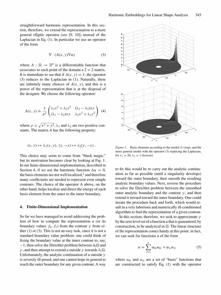
This choice may seem to come from “black magic,”but its motivation becomes clear by looking at Fig. 1.In our finite-dimensional implementation, described inSection 4, if we use the harmonic function �u = 0,the basis elements are not well localized,2 and thereforemany coefficients are needed to represent even simplecontours. The choice of the operator A above, on theother hand, helps localize and direct the energy of eachbasis element from the outer to the inner boundary.
4. Finite-Dimensional Implementation
So far we have managed to avoid addressing the prob-lem of how to compute the representation u (or itsboundary values f0, f1) from the contour γ from ei-ther (1) or (3). This is not an easy task, since it is not astandard boundary value problem: one could think offixing the boundary value at the inner contour to, say,−1, then solve the Dirichlet problem between ∂0� andγ , and then attempt to extend u outside γ towards ∂1�.Unfortunately, the analytic continuation of u outside γ
is severely ill-posed, and one cannot hope in general toreach the outer boundary for any given contour. A way
Figure 1. Basis elements according to the model (1) (top), and themore general model with the operator (3) replacing the Laplacian,for λ1 = 20, λ2 = 1 (bottom).
to fix this would be to carry out the analytic continu-ation as far as possible (until a singularity develops)toward the outer boundary, then smooth the resultinganalytic boundary values. Next, reverse the procedureto solve the Dirichlet problem between the smoothedouter analytic boundary and the contour γ , and thenextend it inward toward the inner boundary. One coulditerate the procedure back and forth, which would re-sult in a very laborious and numerically ill-conditionedalgorithm to find the representation of a given contour.
In this section, therefore, we seek to approximate γ
by the zero level set of a function u that is guaranteed, byconstruction, to be analytical in �. The linear structureof the representation comes handy at this point: in fact,we can seek for functions u of the form
u =n∑
i=1
α0i u0i + α1i u1i (5)
where u0i and u1i are a set of “basis” functions thatare constructed to satisfy Eq. (1) with the operator
346 Duci et al.
(3) replacing the Laplacian, and including the con-straints of Remark 2.2 on the inner and outer boundaryrespectively. More in detail, in order to compute the ba-sis elements, for a chosen positive integer n, we indicatewith {s0 j }1≤ j≤n and {s1 j }1≤ j≤n respectively a partitionof the inner and outer boundary of �, with |si j | thelength of the segment si, j , and seek for {ui j }i=0,1; j=1...n
that solve the following partial differential equation(PDE)⎧⎪⎪⎪⎨⎪⎪⎪⎩
∇ · (A(x, y)∇ui j (x, y)) = 0 for (x, y) ∈ �
ui j (x, y) = 0 for (x, y) ∈ ∂�\si j ,
ui j (x, y) = 1
|si j | for (x, y) ∈ si j .
(6)
We have integrated this PDE numerically using stan-dard finite-element methods [4], and in Fig. 1 weshow sample basis elements for the case of the sim-ple Laplacian A(x, y) = I (top), and the more generalanisotropic operator (4) (bottom).
Note that this PDE needs only to be solved onceand off-line. Once the basis elements are known, eachcontour will be represented by the coefficients {αi j },which can be found following the procedure that wedescribe next.
First, we need to set up a cost functional that mea-sures the discrepancy between the target contour thatwe want to represent, γ , and the model contour that ad-mits a harmonic embedding. A simple cost function issimply the Lebesgue measure of the set symmetric dif-ference3 between the inside of the contour γ , which weindicate with
◦γ , and the set of points that correspond to
a negative value of u, which we indicate by u−. Otherchoices of cost functional are possible, for instancethe Hausdorff distance, and we choose the set sym-metric difference only for simplicity. Now, ideally onewould want to write this functional explicitly in termsof {αi j }, and differentiate it to yield a gradient descentalgorithm. Unfortunately, it is not easy to write the zerolevel set of u as a function of the parameters α. How-ever, one can achieve the same results by first comput-ing the gradient flow of the cost functional with respectto an unconstrained u, then projecting this flow onto thebasis {ui j }. More formally, consider a general infinites-imal contour variation C : [0, 1] × [−ε, ε] → �; thenthe gradient descend evolutions of the symmetric dif-
ference the target set◦γ and the approximating set
◦C is
given by
Ct =(X ◦
γ− 1
2
)N
where N is the outward unit normal at C(·, 0) and X ◦γ
is
the characteristic function of the set◦γ . After project-
ing onto the basis elements ui j via∫
C 〈ut , ui j 〉ds, oneobtains the update formula for the coefficients
α′i j = αi j − μ
∫C(·,0)
ui j
|∇u|(X ◦
γ− 1
2
)d s , (7)
where μ is a positive constant to be chosen as a designparameter. Finally, one has to enforce the conditions onthe sign at the boundary value, described in Proposition2.1; in this case we simply have:
α0 j < 0, α1 j > 0 ∀ j ∈ {1, . . . , n} .
We obtain the normalization, with respect to the scalefactor of the Remark 2.2, dividing by
∑i=1,2; j=1,... ,n
|αi, j |.
Given a target contour γ , this procedure allows us toestimate its representation αi, j . In the next section wepresent some experiments that illustrate the features ofthis representation.
5. Application to Thickness Estimationfor Annular Tissues
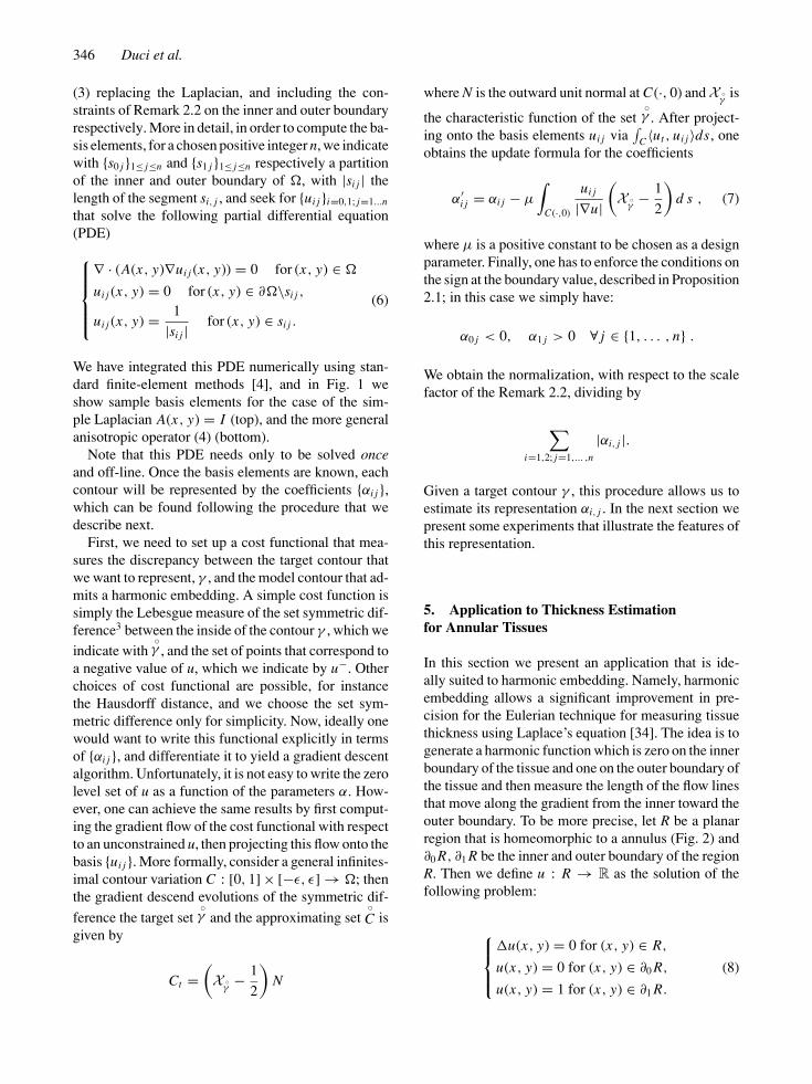
In this section we present an application that is ide-ally suited to harmonic embedding. Namely, harmonicembedding allows a significant improvement in pre-cision for the Eulerian technique for measuring tissuethickness using Laplace’s equation [34]. The idea is togenerate a harmonic function which is zero on the innerboundary of the tissue and one on the outer boundary ofthe tissue and then measure the length of the flow linesthat move along the gradient from the inner toward theouter boundary. To be more precise, let R be a planarregion that is homeomorphic to a annulus (Fig. 2) and∂0 R, ∂1 R be the inner and outer boundary of the regionR. Then we define u : R → R as the solution of thefollowing problem:
⎧⎪⎨⎪⎩�u(x, y) = 0 for (x, y) ∈ R,
u(x, y) = 0 for (x, y) ∈ ∂0 R,
u(x, y) = 1 for (x, y) ∈ ∂1 R.
(8)
Harmonic Embeddings for Linear Shape Analysis 347
Figure 2. Inner and outer boundaries of the tissue region R and acorrespondence trajectory.
To each point x ∈ R, one then associates the uniquetrajectory which passes trough x and which is tangentto the normalized gradient vector field
T = ∇u
|∇u| .
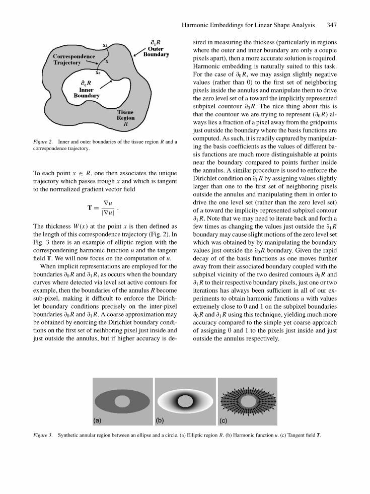
The thickness W (x) at the point x is then defined asthe length of this correspondence trajectory (Fig. 2). InFig. 3 there is an example of elliptic region with thecorrespondening harmonic function u and the tangentfield T. We will now focus on the computation of u.
When implicit representations are employed for theboundaries ∂0 R and ∂1 R, as occurs when the boundarycurves where detected via level set active contours forexample, then the boundaries of the annulus R becomesub-pixel, making it difficult to enforce the Dirich-let boundary conditions precisely on the inter-pixelboundaries ∂0 R and ∂1 R. A coarse approximation maybe obtained by enorcing the Dirichlet boundary condi-tions on the first set of neihboring pixel just inside andjust outside the annulus, but if higher accuracy is de-
Figure 3. Synthetic annular region between an ellipse and a circle. (a) Elliptic region R. (b) Harmonic function u. (c) Tangent field T.
sired in measuring the thickess (particularly in regionswhere the outer and inner boundary are only a couplepixels apart), then a more accurate solution is required.Harmonic embedding is naturally suited to this task.For the case of ∂0 R, we may assign slightly negativevalues (rather than 0) to the first set of neighboringpixels inside the annulus and manipulate them to drivethe zero level set of u toward the implicitly representedsubpixel countour ∂0 R. The nice thing about this isthat the countour we are trying to represent (∂0 R) al-ways lies a fraction of a pixel away from the gridpointsjust outside the boundary where the basis functions arecomputed. As such, it is readily captured by manipulat-ing the basis coefficients as the values of different ba-sis functions are much more distinguishable at pointsnear the boundary compared to points further insidethe annulus. A similar procedure is used to enforce theDirichlet condition on ∂1 R by assigning values slightlylarger than one to the first set of neighboring pixelsoutside the annulus and manipulating them in order todrive the one level set (rather than the zero level set)of u toward the implicity represented subpixel contour∂1 R. Note that we may need to iterate back and forth afew times as changing the values just outside the ∂1 Rboundary may cause slight motions of the zero level setwhich was obtained by by manipulating the boundaryvalues just outside the ∂0 R boundary. Given the rapiddecay of of the basis functions as one moves furtheraway from their associated boundary coupled with thesubpixel vicinity of the two desired contours ∂0 R and∂1 R to their respective boundary pixels, just one or twoiterations has always been sufficient in all of our ex-periments to obtain harmonic functions u with valuesextremely close to 0 and 1 on the subpixel boundaries∂0 R and ∂1 R using this technique, yielding much moreaccuracy compared to the simple yet coarse approachof assigning 0 and 1 to the pixels just inside and justoutside the annulus respectively.
348 Duci et al.
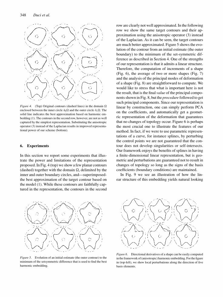
Figure 4. (Top) Original contours (dashed lines) in the domain �
enclosed between the inner circle ∂0� and the outer circle ∂1�. Thesolid line indicates the best approximation based on harmonic em-bedding (1). The contours in the second row, however, are not as wellcaptured by the simplest representation. Substituting the anisotropicoperator (3) instead of the Laplacian results in improved representa-tional power of our scheme (bottom).
6. Experiments
In this section we report some experiments that illus-trate the power and limitations of the representationproposed. In Fig. 4 (top) we show a few planar contours(dashed) together with the domain �, delimited by theinner and outer boundary circles, and—superimposed-the best approximation of the target contour based onthe model (1). While these contours are faithfully cap-tured in the representation, the contours in the second
Figure 5. Evolution of an initial estimate (the outer contour) to theminimum of the setsymmetric difference that is used to find the bestharmonic embedding.
row are clearly not well approximated. In the followingrow we show the same target contours and their ap-proximation using the anisotropic operator (3) insteadof the Laplacian. As it can be seen, the target contoursare much better approximated. Figure 5 shows the evo-lution of the contour from an initial estimate (the outerboundary) to the minimum of the set-symmetric dif-ference as described in Section 4. One of the strengthsof our representation is that it admits a linear structure.Therefore, the computation of increments of a shape(Fig. 6), the average of two or more shapes (Fig. 7)and the analysis of the principal modes of deformationof a shape (Fig. 8) are straightforward to compute. Wewould like to stress that what is important here is notthe result, that is the final value of the principal compo-nents shown in Fig. 8, but the procedure followed to getsuch principal components. Since our representation islinear by construction, one can simply perform PCAon the coefficients, and automatically get a geomet-ric representation of the deformation that guaranteesthat no changes of topology occur. Figure 6 is perhapsthe most crucial one to illustrate the features of ourmethod. In fact, if we were to use parametric represen-tations of a curve, for instance splines, by perturbingthe control points we are not guaranteed that the con-tour does not develop singularities or self-intersects.Our framework enjoys the benefits of splines in havinga finite-dimensional linear representation, but is geo-metric and perturbations are guaranteed not to result inchanges of topology so long as the signs of the basiscoefficients (boundary conditions) are maintained.
In Fig. 9 we see an illustration of how the lin-ear structure of this embedding yields natural looking
Figure 6. Directional derivatives of a shape can be easily computedin the framework of (anisotropic) harmonic embedding. For the figurein (top-left), we show local perturbations along the direction of fivebasis elements.
Harmonic Embeddings for Linear Shape Analysis 349
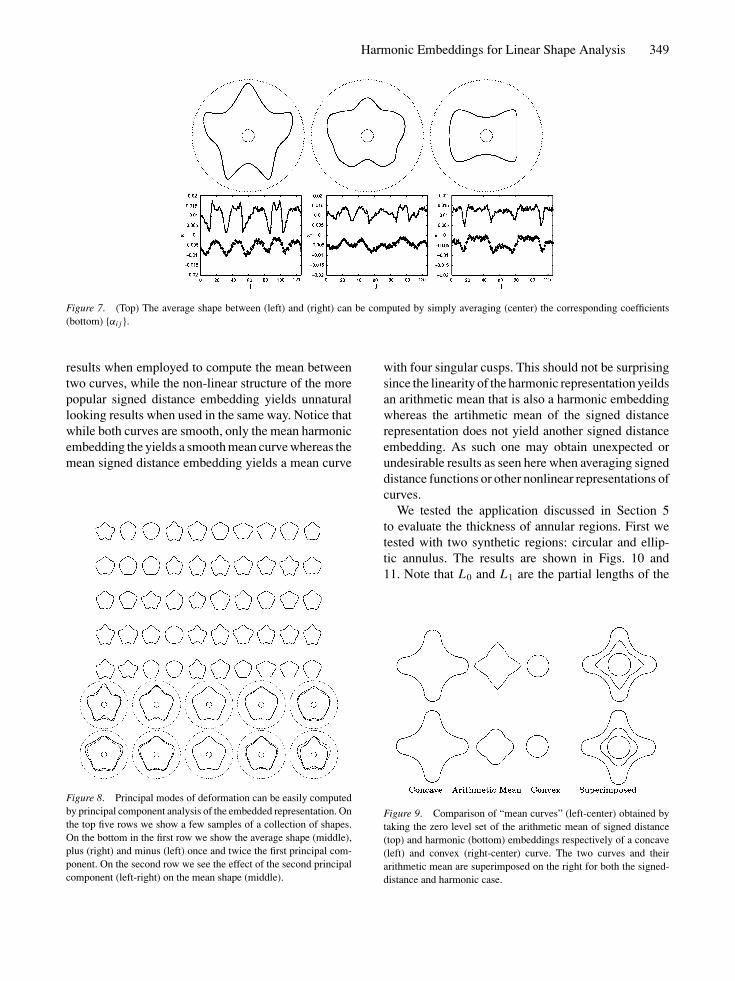
Figure 7. (Top) The average shape between (left) and (right) can be computed by simply averaging (center) the corresponding coefficients(bottom) {αi j }.
results when employed to compute the mean betweentwo curves, while the non-linear structure of the morepopular signed distance embedding yields unnaturallooking results when used in the same way. Notice thatwhile both curves are smooth, only the mean harmonicembedding the yields a smooth mean curve whereas themean signed distance embedding yields a mean curve
Figure 8. Principal modes of deformation can be easily computedby principal component analysis of the embedded representation. Onthe top five rows we show a few samples of a collection of shapes.On the bottom in the first row we show the average shape (middle),plus (right) and minus (left) once and twice the first principal com-ponent. On the second row we see the effect of the second principalcomponent (left-right) on the mean shape (middle).
with four singular cusps. This should not be surprisingsince the linearity of the harmonic representation yeildsan arithmetic mean that is also a harmonic embeddingwhereas the artihmetic mean of the signed distancerepresentation does not yield another signed distanceembedding. As such one may obtain unexpected orundesirable results as seen here when averaging signeddistance functions or other nonlinear representations ofcurves.
We tested the application discussed in Section 5to evaluate the thickness of annular regions. First wetested with two synthetic regions: circular and ellip-tic annulus. The results are shown in Figs. 10 and11. Note that L0 and L1 are the partial lengths of the
Figure 9. Comparison of “mean curves” (left-center) obtained bytaking the zero level set of the arithmetic mean of signed distance(top) and harmonic (bottom) embeddings respectively of a concave(left) and convex (right-center) curve. The two curves and theirarithmetic mean are superimposed on the right for both the signed-distance and harmonic case.

350 Duci et al.
Figure 10. Thickness computations for a synthetic annular regionbetween two concentric circles. (a) Circular annulus. (b) Harmonicfunction u. (c) Tangent Field. T. (d) Length L0. (e) Length L1. (f)Thickness (L0 + L1).
Figure 11. Thickness computations for a synthetic region betweenan ellipse and a circle. (a) Length L0. (b) Length L1. (c) Thickness(L0 + L1).
corresponding flow trajectories between each point xand the boundaries ∂0 R and ∂1 R respectively whilethe thickness is defined by the total trajectory lengthL0 + L1. We tested the method also on a segmenta-tion of the myocardium obtained from a short-axis MRimage of the heart shown in Fig. 12(a).
Finally, we applied the harmonic embedding repre-sentation to a couple of 3-D contours within a sphericalannulus. Figures 13 and 14 show the 3-D evolutions ofthe contours from the initial estimates to the target con-tours that we want to represent. Figure 15 shows the av-erage shape obtained by just averaging the coefficients.In addition, convex combinations of the harmonic em-bedding representations can be easily computed by justdoing a weighted average of the coefficients to contin-uously interpolate between the two shapes (Fig. 16).
Figure 12. Myocardial thickness from a short-axis MR image. (a) Endocardial and epicardial contours. (b) Tangent field. (c) Boundarycorrespondences for some selected points. (d) Thickness.
Figure 13. Evolution of an initial estimate to the minimum of theset-symmetric difference that is used to find the best harmonic em-bedding. (a) Initial contour estimate. (b)–(e) Evolutions. (f) Targetcontour.
Figure 14. Evolution of an initial estimate to the minimum of theset-symmetric difference that is used to find the best harmonic em-bedding. (a) Initial contour estimate. (b)–(e) Evolutions. (f) Targetcontour.
Figure 15. Average shape between (left) and (right) computed bysimply averaging (center) the corresponding coefficients.
Harmonic Embeddings for Linear Shape Analysis 351
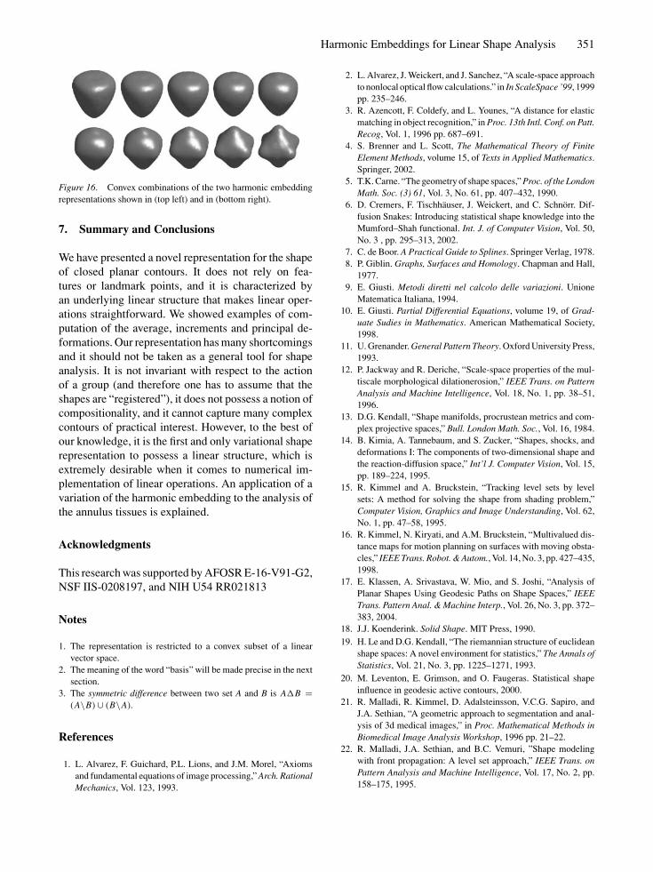
Figure 16. Convex combinations of the two harmonic embeddingrepresentations shown in (top left) and in (bottom right).
7. Summary and Conclusions
We have presented a novel representation for the shapeof closed planar contours. It does not rely on fea-tures or landmark points, and it is characterized byan underlying linear structure that makes linear oper-ations straightforward. We showed examples of com-putation of the average, increments and principal de-formations. Our representation has many shortcomingsand it should not be taken as a general tool for shapeanalysis. It is not invariant with respect to the actionof a group (and therefore one has to assume that theshapes are “registered”), it does not possess a notion ofcompositionality, and it cannot capture many complexcontours of practical interest. However, to the best ofour knowledge, it is the first and only variational shaperepresentation to possess a linear structure, which isextremely desirable when it comes to numerical im-plementation of linear operations. An application of avariation of the harmonic embedding to the analysis ofthe annulus tissues is explained.
Acknowledgments
This research was supported by AFOSR E-16-V91-G2,NSF IIS-0208197, and NIH U54 RR021813
Notes
1. The representation is restricted to a convex subset of a linearvector space.
2. The meaning of the word “basis” will be made precise in the nextsection.
3. The symmetric difference between two set A and B is A�B =(A\B) ∪ (B\A).
References
1. L. Alvarez, F. Guichard, P.L. Lions, and J.M. Morel, “Axiomsand fundamental equations of image processing,” Arch. RationalMechanics, Vol. 123, 1993.
2. L. Alvarez, J. Weickert, and J. Sanchez, “A scale-space approachto nonlocal optical flow calculations.” in In ScaleSpace ’99, 1999pp. 235–246.
3. R. Azencott, F. Coldefy, and L. Younes, “A distance for elasticmatching in object recognition,” in Proc. 13th Intl. Conf. on Patt.Recog, Vol. 1, 1996 pp. 687–691.
4. S. Brenner and L. Scott, The Mathematical Theory of FiniteElement Methods, volume 15, of Texts in Applied Mathematics.Springer, 2002.
5. T.K. Carne. “The geometry of shape spaces,” Proc. of the LondonMath. Soc. (3) 61, Vol. 3, No. 61, pp. 407–432, 1990.
6. D. Cremers, F. Tischhauser, J. Weickert, and C. Schnorr. Dif-fusion Snakes: Introducing statistical shape knowledge into theMumford–Shah functional. Int. J. of Computer Vision, Vol. 50,No. 3 , pp. 295–313, 2002.
7. C. de Boor. A Practical Guide to Splines. Springer Verlag, 1978.8. P. Giblin. Graphs, Surfaces and Homology. Chapman and Hall,
1977.9. E. Giusti. Metodi diretti nel calcolo delle variazioni. Unione
Matematica Italiana, 1994.10. E. Giusti. Partial Differential Equations, volume 19, of Grad-
uate Sudies in Mathematics. American Mathematical Society,1998.
11. U. Grenander. General Pattern Theory. Oxford University Press,1993.
12. P. Jackway and R. Deriche, “Scale-space properties of the mul-tiscale morphological dilationerosion,” IEEE Trans. on PatternAnalysis and Machine Intelligence, Vol. 18, No. 1, pp. 38–51,1996.
13. D.G. Kendall, “Shape manifolds, procrustean metrics and com-plex projective spaces,” Bull. London Math. Soc., Vol. 16, 1984.
14. B. Kimia, A. Tannebaum, and S. Zucker, “Shapes, shocks, anddeformations I: The components of two-dimensional shape andthe reaction-diffusion space,” Int’l J. Computer Vision, Vol. 15,pp. 189–224, 1995.
15. R. Kimmel and A. Bruckstein, “Tracking level sets by levelsets: A method for solving the shape from shading problem,”Computer Vision, Graphics and Image Understanding, Vol. 62,No. 1, pp. 47–58, 1995.
16. R. Kimmel, N. Kiryati, and A.M. Bruckstein, “Multivalued dis-tance maps for motion planning on surfaces with moving obsta-cles,” IEEE Trans. Robot. & Autom., Vol. 14, No. 3, pp. 427–435,1998.
17. E. Klassen, A. Srivastava, W. Mio, and S. Joshi, “Analysis ofPlanar Shapes Using Geodesic Paths on Shape Spaces,” IEEETrans. Pattern Anal. & Machine Interp., Vol. 26, No. 3, pp. 372–383, 2004.
18. J.J. Koenderink. Solid Shape. MIT Press, 1990.19. H. Le and D.G. Kendall, “The riemannian structure of euclidean
shape spaces: A novel environment for statistics,” The Annals ofStatistics, Vol. 21, No. 3, pp. 1225–1271, 1993.
20. M. Leventon, E. Grimson, and O. Faugeras. Statistical shapeinfluence in geodesic active contours, 2000.
21. R. Malladi, R. Kimmel, D. Adalsteinsson, V.C.G. Sapiro, andJ.A. Sethian, “A geometric approach to segmentation and anal-ysis of 3d medical images,” in Proc. Mathematical Methods inBiomedical Image Analysis Workshop, 1996 pp. 21–22.
22. R. Malladi, J.A. Sethian, and B.C. Vemuri, ”Shape modelingwith front propagation: A level set approach,” IEEE Trans. onPattern Analysis and Machine Intelligence, Vol. 17, No. 2, pp.158–175, 1995.
352 Duci et al.
23. K.V. Mardia and I.L. Dryden, “Shape distributions for landmarkdata,” Adv. appl. prob., Vol. 21, No. 4, pp. 742–755, 1989.
24. G. Matheron. Random Sets and Integral Geometry. Wiley, 1975.25. M.I. Miller and L. Younes, “Group action, diffeomorphism and
matching: A general framework. In Proc. of SCTV, 1999.26. D. Mumford, “Mathematical theories of shape: Do they model
perception?” In Geometric methods in computer vision, Vol.1570, pp. 2–10, 1991.
27. S. Osher and J. Sethian, “Fronts propagating with curvature-dependent speed: Algorithms based on hamilton-jacobi equa-tions,” J. of Camp. Physics, Vol. 79, pp. 12–49, 1988.
28. C. Samson, L. Blanc-Feraud, G. Aubert, and J. Zerubia, “A levelset model for image classification,” in International Conferenceon Scale-Space Theories in Computer Vision, 1999 pp. 306–317.
29. E. Sharon and D. Mumford, “2D-Shape Analysis using Confor-mal Mapping,” in Conference on Computer Vision and PatternRecognition, 2004.
30. B. ter Haar Romeny, L. Florack, J. Koenderink, and M.V.(Eds.), “Scale-space theory in computer vision,” in Lecture
Notes in Computer Science, Vol. 1252. Springer Verlag,1997.
31. R. Thom. Structural Stability and Morphogenesis. Benjamin;Reading, 1975.
32. D.W. Thompson. On Growth and Form. Dover, 1917.33. P. Thompson and A.W. Toga, “A surface-based technique for
warping three-dimensional images of the brain,” IEEE Trans.Med. Imaging, Vol. 15, No. 4, pp. 402–417, 1996.
34. A. Yezzi and J. Prince, “An eulerian pde approach for computingtissue thicknes,” IEEE Trans. Medical Imaging, Vol. 22, pp.1332–1339, 2003.
35. A. Yezzi and S. Soatto, “Stereoscopic segmentation,” in Proc.of the Intl. Conf. on Computer Vision, 2001 pp. 59–66.
36. A. Yezzi and S. Soatto, “Deformotion: Deforming motion, shapeaverage and the joint segmentation and registration of images,”Intl. J. of Comp. Vis., accepted, 2003.
37. L. Younes, “Computable elastic distances between shapes,”SIAM J. of Appl. Math., 1998.
38. A. Yuille. “Deformable templates for face recognition.” J. ofCognitive Neurosci., Vol. 3, No. 1, pp. 59–70, 1991.