November 10, 2017 9:10 WSPC/S0218-1274 1730037

International Journal of Bifurcation and Chaos, Vol. 27, No. 11 (2017) 1730037 (19 pages)c© World Scientific Publishing CompanyDOI: 10.1142/S0218127417300373

Harmonic Oscillators with Nonlinear Damping

J. C. SprottDepartment of Physics, University of Wisconsin-Madison,

Madison, Wisconsin 53706, USAsprott@physics.wisc.edu

W. G. HooverRuby Valley Research Institute, Highway Contract 60,

Box 601, Ruby Valley, Nevada 89833, USAhooverwilliam@yahoo.com

Received September 10, 2017

Dynamical systems with special properties are continually being proposed and studied. Manyof these systems are variants of the simple harmonic oscillator with nonlinear damping. Thispaper characterizes these systems as a hierarchy of increasingly complicated equations withcorrespondingly interesting behavior, including coexisting attractors, chaos in the absence ofequilibria, and strange attractor/repellor pairs.

Keywords : Chaos; harmonic oscillator; attractors; dissipation; ergodicity.

1. Introduction

The stable periodic motion of the simple harmonicoscillator provides an ideal test bed for numericalintegrators as well as a launch pad for more compli-cated chaotic dynamical systems in three or moredimensions. The equations of motion produce a cir-cular orbit in phase space that can be used to testand compare numerical integration methods thatare still being developed.

Long ago, Gibbs [1902] predicted that such anoscillator when driven by random thermal fluctu-ations should have a Gaussian probability densityin phase space. That prediction motivated a searchfor nonlinear modifications to the simple harmonicoscillator that would generate such a Gaussian dis-tribution rather than the simple one-dimensionalcircle. Because chaos is a necessary ingredient forpopulating the phase space and replicating thermalrandomness, the research has necessarily been car-ried out in three or more dimensions rather thantwo and has uncovered some unexpected mathe-matical results of interest to the dynamical systemscommunity.

This work provides a summary of the gener-alizations and observations based on autonomousharmonic oscillators of the form

x = y,

y = −x − fy(1)

where the damping coefficient f is a functional of(x, y) and additional variables and their integrals asrequired in higher dimensions and that controls thedissipation which can be positive or negative. Webegin with an analysis of two-dimensional systemswhere the solutions are regular, and then extend theresults to higher dimensions where chaos and newless familiar phenomena occur.

2. Two-Dimensional Systems

2.1. Simple harmonic oscillator

The simplest nontrivial dynamical system is thesimple harmonic oscillator,

x = y,

y = −x,

(2)

1730037-1

Int.

J. B

ifur

catio

n C

haos

201

7.27

. Dow

nloa

ded

from

ww

w.w

orld

scie

ntif

ic.c

omby

CIT

Y U

NIV

ER

SIT

Y O

F H

ON

G K

ON

G o

n 11

/22/

17. F

or p

erso

nal u

se o

nly.

November 10, 2017 9:10 WSPC/S0218-1274 1730037

J. C. Sprott & W. G. Hoover

which might, for example, model the motion of amass on an ideal spring where x would representthe displacement of the mass from its equilibriumposition and y would represent its velocity. For sim-plicity, and without loss of generality, the mass andspring constant have been set to unity.

Note that in the physics literature, the phasespace variables (x, y) are customarily written as(q, p) or sometimes as (x, v). We use the more gen-eral notation to emphasize that oscillations occur inmany contexts that do not involve moving massesand velocities, such as electrical circuits [Buscarinoet al., 2014], musical instruments [Fletcher & Ross-ing, 1998], population dynamics [Murray, 1989],economics [Mishchenko, 2014], chemical clock reac-tions [Epstein & Pojman, 1998], and many others.

The only equilibrium of Eq. (2) is at the origin(x, y) = (0, 0), and it is neutrally stable with eigen-values ±i, which means that nearby (in fact all)solutions oscillate sinusoidally with a frequency of1 radian per unit time forming concentric circles in(x, y) space centered on the origin with radii thatdepend on the initial conditions. Thus the origin iscalled a center, and the surrounding circular orbitshave a radius r given by r2 = x2 + y2.

This system is conservative, both in the sensethat the total energy (potential 1

2x2 plus kinetic12y2) is constant, and in the sense that the area occu-pied by a cluster of initial conditions as they evolvein time is constant (Liouville’s theorem). Thus theflow, represented by the collection of all possibleorbits, is incompressible. This system is also thesimplest example of a Hamiltonian system with aHamiltonian given by H = 1

2x2 + 12y2 from which

the equations of motion can be derived using Hamil-ton’s motion equations x = ∂H

∂y and y = −∂H∂x .

Finally, the system is time-reversible, asexpected for a conservative system, since the trans-formation (x, y, t) → (x,−y,−t) or (x, y, t) → (−x,y,−t) leaves the equations unchanged. Another wayof reversing the direction of time is to change thesign of ∆t in the numerical integrator, which givesthe same circular orbit but traversed in a counter-clockwise rather than a clockwise direction.

2.2. Linearly-damped harmonicoscillator

In the real world, all classical harmonic oscillatorshave some form of damping that converts theirmechanical energy into heat and eventually brings

the system to rest. The simplest way to representsuch an effect is to add a linear term −by to the sim-ple harmonic oscillator corresponding to a frictionalforce that is proportional to the velocity,

x = y,

y = −x − by.(3)

The resulting system is called a damped har-monic oscillator, and b (if positive) is the damp-ing constant. It describes the exponential rate atwhich orbits spiral into the origin at (0, 0) and isrelated to the Q (quality) factor of the oscillatorby b = 1/Q. The Q of an oscillator is the numberof radians of oscillation required for the energy todecay to 1/e of its original value. A system withQ = 1/2 (or b = 2) is critically damped, and smallervalues of Q (or b > 2) do not oscillate, but theyrapidly approach the origin.

It seems that it should be possible to eliminatethe b in Eq. (3) by a linear rescaling of x, y, and t,but that cannot be done as simple algebra shows.This system is special in that it has two distincttime-scales, the damping rate and the frequencyof oscillation, and the parameter b controls theirratio.

The origin is a stable equilibrium with eigenval-ues −b/2 ± √

b2/4 − 1. For underdamped systems(b < 2), the equilibrium is a called a focus, and foroverdamped systems (b > 2), it is called a node.A stable equilibrium is the simplest example of anattractor since orbits starting from nearby initialconditions are drawn to it as time advances. In fact,this system is a global attractor since all initial con-ditions are drawn to it. Its basin of attraction isthe whole of phase space, a so-called class 1a basinaccording to Sprott and Xiong [2015].

The damped harmonic oscillator is a dissipativesystem. Furthermore, it is not time-reversible forb > 0 since reversing the sign of t in the equationsconverts the attractor into a repellor and causes theorbits to spiral outward to infinity (we say the time-reversed system is unbounded).

Normally systems with dissipation such as thisare not considered to be Hamiltonian, but the time-dependent Hamiltonian H = 1

2(x2e+t +y2e−t) givesthe equations of motion x = ye−t and y = −xe+t,so that a chain rule evaluation of x gives x =ddt(ye−t) = ye−t − ye−t = −x− x, the motion equa-tion of an underdamped harmonic oscillator withb = 1. The orbit is a spiral in (x, y) space ending atthe origin.

1730037-2

Int.

J. B

ifur

catio

n C

haos

201

7.27

. Dow

nloa

ded

from

ww

w.w

orld

scie

ntif

ic.c

omby

CIT

Y U

NIV

ER

SIT

Y O

F H

ON

G K

ON

G o

n 11

/22/

17. F

or p

erso

nal u

se o

nly.

November 10, 2017 9:10 WSPC/S0218-1274 1730037

Harmonic Oscillators with Nonlinear Damping

2.3. Nonlinearly-damped harmonicoscillator

More complicated damping functions are also possi-ble. For example, the damping could be cubic ratherthan linear,

x = y,

y = −x − by3.(4)

The origin (0, 0) is still an attractor for b > 0, butthis is not evident since the eigenvalues are ±i justas for the simple harmonic oscillator in Eq. (2).Nearby orbits are attracted to it, but they approachit more slowly than a decaying exponential. We saythe equilibrium is nonlinearly stable, and a morecomplicated analysis is required to determine itsstability.

Such an analysis usually involves a transforma-tion of variables to polar coordinates (r, θ), wherer2 = x2 + y2 and θ = arctan(y/x). Differentiatingr2 with respect to time gives rr = xx + yy = −by4.Then the stability is determined by the sign of− b

ry4, which is always negative for b > 0 since y4

is always positive. Thus the distance of the orbitfrom the origin decreases monotonically in time.In fact, given that the orbit is nearly circular andsinusoidal near the origin for b small, it followsfrom the integration of y4 = (r sin θ)4 over onecycle that 〈y4〉 = 3r4/8, from which the differen-tial equation becomes r = −3br3/8, whose solutionis r = ( 1

r20

+ 3bt4 )−1/2 or r ≈ 2/

√3bt for t → ∞.

For more complicated cases, or in higher dimen-sions where the real parts of the eigenvalues arezero, it may be easier to check the stability numeri-cally by taking an initial condition in the vicinity ofthe equilibrium and see if the orbits get closer to itor farther from it as time advances. However, thiscan be difficult if the orbit is noncircular becausethe distance will itself oscillate, and it is necessaryto follow the orbit for exactly one cycle or for a verylong time.

This is a good time to mention the importanceof using an accurate numerical integrator. In par-ticular, the popular fourth-order Runge–Kutta inte-grator is known to introduce a spurious numericaldamping proportional to the fifth power of the stepsize ∆t, such that a solution of the simple har-monic oscillator in Eq. (2) behaves like the lin-early damped harmonic oscillator of Eq. (3) withb = (∆t)5/5! for ∆t 1. The fifth-order Runge–Kutta integrator produces a similar antidamping

given by b = −(∆t)6/6! for ∆t 1. This is typ-ically not an issue for dissipative systems that havean attractor, but for conservative systems, an inte-grator with an adaptive step size and stringent errorcontrol is recommended [Press et al., 1992].

2.4. van der Pol oscillator

Another famous and very old system with nonlineardamping is the van der Pol oscillator [van der Pol,1920, 1926],

x = y,

y = −x − b(x2 − 1)y,(5)

which was originally proposed as a model of oscilla-tions in electronic circuits but has been applied toa wide variety of other phenomena including heart-beats [van der Pol & van der Mark, 1928], sunspotcycles [Passos & Lopes, 2008], and pulsating starscalled Cepheids [Krogdahl, 1955]. Unlike the pre-vious systems, the van der Pol oscillator requiresan external source of energy to maintain the oscil-lations, and this energy is coming from whateverproduces the antidamping represented by the +bypositive feedback term.

For b > 0, the origin is an unstable equilib-rium (a repellor) with eigenvalues b/2±√

b2/4 − 1.Nearby orbits are antidamped, causing the ampli-tude of the oscillations to grow until the time aver-age of 〈x + b(x2 − 1)y〉 = 0, which occurs for〈x2〉 = 〈y2〉 ≈ 2.0594 when b = 1. The resulting tra-jectory in state space is a kind of periodic attractorcalled a limit cycle. The existence and uniquenessof such a limit cycle follows from Lienard ’s theorem[Perko, 1991], which simply states that if the damp-ing is negative for all small values of x and positivefor all large values, the orbit for such an oscillatorhas nowhere else to go but to a limit cycle.

This limit cycle is a global attractor since allinitial conditions are drawn to it except for the sin-gle equilibrium point at the origin (a class 1a basin).The orbit in (x, y) space oscillates back and forthacross a circle of radius 2 twice per cycle. The limitcycle attractor for the system with b = 1 is shown inFig. 1 with the unstable equilibrium shown as a bluedot at the origin. This limit cycle is a self-excitedattractor according to Leonov and Kuznetsov [2013]since initial conditions in the neighborhood of theunstable equilibrium are drawn to it.

The stability of a limit cycle is determined bythe Lyapunov exponents [Wolf et al., 1985; Geist

1730037-3

Int.

J. B

ifur

catio

n C

haos

201

7.27

. Dow

nloa

ded

from

ww

w.w

orld

scie

ntif

ic.c

omby

CIT

Y U

NIV

ER

SIT

Y O

F H

ON

G K

ON

G o

n 11

/22/

17. F

or p

erso

nal u

se o

nly.

November 10, 2017 9:10 WSPC/S0218-1274 1730037

J. C. Sprott & W. G. Hoover

Fig. 1. Limit cycle for the van der Pol oscillator in Eq. (5)with b = 1. The blue dot at the origin is the unstable equi-librium, and the colors along the orbit are the local valuesof the largest Lyapunov exponent with red positive and bluenegative.

et al., 1990], which play the same role for a peri-odic orbit as do the eigenvalues for an equilibriumpoint. For a two-dimensional system such as Eq. (5),there are two Lyapunov exponents, one of which,corresponding to the direction parallel to the orbit,must be zero for an oscillating continuous-time flow.The sum of the Lyapunov exponents is equal to thetime average of the trace of the Jacobian matrix,which for Eq. (5) is b(1 − 〈x2〉) ≈ −1.0594 whenb = 1. Thus the Lyapunov exponents for the vander Pol system with b = 1 are (0,−1.0594). Apositive Lyapunov exponent would indicate thatthe system is chaotic, but that is not possible fora two-dimensional continuous-time system becausethe orbit must not intersect itself as formalizedin the Poincare–Bendixson theorem [Hirsch et al.,2004].

The Lyapunov exponents are determined by atime average of the rate of separation of nearby tra-jectories over one cycle of the limit cycle. Althoughthe largest exponent for a limit cycle must averageto zero, its local value varies greatly over the orbit,ranging from approximately −3.0345 to 2.8138 forEq. (5) with b = 1. This variation is indicated inFig. 1 and the following figures by a color scale inwhich the negative values are in a shade of blue andthe positive values are in a shade of red.

The van der Pol oscillator is not time-reversible.When time is reversed, the repellor at the originbecomes an attractor, and the attracting limit cyclebecomes a repellor. Such attractor/repellor pairs are

common in dynamical systems and will play animportant and perhaps unexpected role in the morecomplicated systems to follow.

2.5. Periodically-damped oscillator

Slightly more interesting behavior occurs if the 1−x2 factor in Eq. (5) is replaced with cos x [Kahn &Zarmi, 1998; Sprott et al., 2017] giving

x = y,

y = −x + by cos x.(6)

For small values of x, the behavior resembles thevan der Pol oscillator, which is not surprising sincethe Taylor series expansion (more properly called aMaclaurin series since it is centered at x = 0) ofthe cosine function is cos x = 1 − 1

2x2 + 124x4 − · · · .

The origin is an unstable equilibrium (a repellor)with the same eigenvalues as for the van der Poloscillator.

However, for larger values of x, the system hasannular regions of alternating damping and anti-damping, giving rise to an infinite series of nestedlimit cycles, the first four of which for b = 1 areshown as black curves in Fig. 2. The second Lya-punov exponent (the damping) for the four cases are(−0.4090,−0.2522,−0.1978,−0.1680), respectively,and the first Lyapunov exponent is zero as requiredfor a limit cycle. Each limit cycle resides withina finite-sized basin of attraction (a class 4 basin)as shown with different colors in the figure. The

Fig. 2. The first four of infinitely many limit cycles (inblack) for the periodically-damped oscillator in Eq. (6) withb = 1 along with their basins of attraction (in colors). Theblue dot at the origin is the unstable equilibrium.

1730037-4

Int.

J. B

ifur

catio

n C

haos

201

7.27

. Dow

nloa

ded

from

ww

w.w

orld

scie

ntif

ic.c

omby

CIT

Y U

NIV

ER

SIT

Y O

F H

ON

G K

ON

G o

n 11

/22/

17. F

or p

erso

nal u

se o

nly.

November 10, 2017 9:10 WSPC/S0218-1274 1730037

Harmonic Oscillators with Nonlinear Damping

boundary between each basin is a repellor, and ini-tial conditions in its vicinity take a long time toreach one of the limit cycles.

This is an example of a multistable system withcoexisting attractors. The innermost limit cycle isself-excited since it can be found by starting withan initial condition in the neighborhood of the equi-librium at the origin, but the others are hidden[Leonov & Kuznetsov, 2013] and require a carefulselection of initial conditions such as (nπ, 0), wheren = 1, 3, 5, 7, . . . .

When time is reversed, the repellor at theorigin becomes an attractor, and all the limitcycles become repellors, forming the basin bound-aries of the new adjacent attractors. Furthermore,the repelling boundaries between the limit cyclesbecome limit-cycle attractors, giving a plot similarto the one in Fig. 2. This is a system with infinitelymany attractor/repellor pairs of ever increasingenergy, reminiscent of the orbitals in an atom.

2.6. Rayleigh oscillator

A similar system to the van der Pol oscillator is theRayleigh oscillator [Birkhoff & Rota, 1978] in whichthe x2 damping factor in Eq. (5) for the van der Poloscillator is replaced by y2,

x = y,

y = −x − b(y2 − 1)y.(7)

In fact, Eq. (5) can be derived from Eq. (7) by dif-ferentiating each term with respect to time and thenreplacing x with x and y with y.

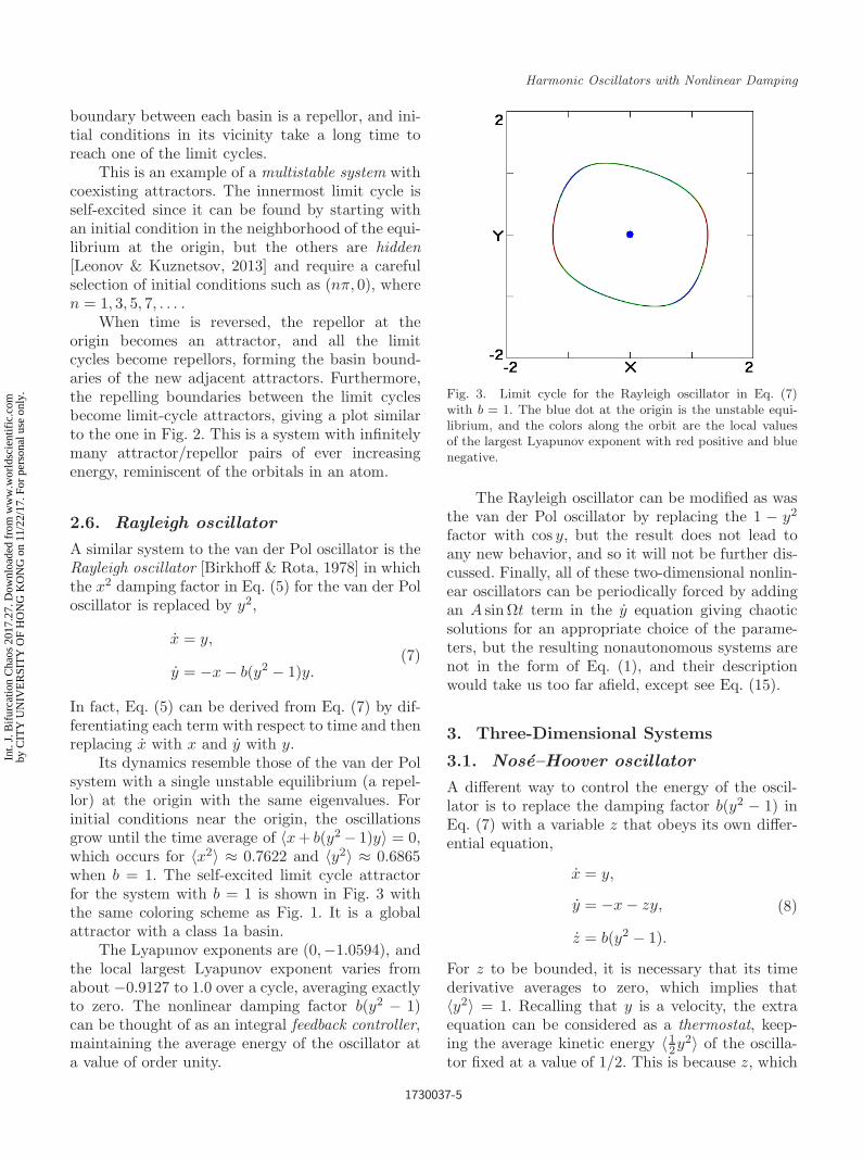
Its dynamics resemble those of the van der Polsystem with a single unstable equilibrium (a repel-lor) at the origin with the same eigenvalues. Forinitial conditions near the origin, the oscillationsgrow until the time average of 〈x + b(y2 − 1)y〉 = 0,which occurs for 〈x2〉 ≈ 0.7622 and 〈y2〉 ≈ 0.6865when b = 1. The self-excited limit cycle attractorfor the system with b = 1 is shown in Fig. 3 withthe same coloring scheme as Fig. 1. It is a globalattractor with a class 1a basin.

The Lyapunov exponents are (0,−1.0594), andthe local largest Lyapunov exponent varies fromabout −0.9127 to 1.0 over a cycle, averaging exactlyto zero. The nonlinear damping factor b(y2 − 1)can be thought of as an integral feedback controller,maintaining the average energy of the oscillator ata value of order unity.

Fig. 3. Limit cycle for the Rayleigh oscillator in Eq. (7)with b = 1. The blue dot at the origin is the unstable equi-librium, and the colors along the orbit are the local valuesof the largest Lyapunov exponent with red positive and bluenegative.

The Rayleigh oscillator can be modified as wasthe van der Pol oscillator by replacing the 1 − y2

factor with cos y, but the result does not lead toany new behavior, and so it will not be further dis-cussed. Finally, all of these two-dimensional nonlin-ear oscillators can be periodically forced by addingan A sin Ωt term in the y equation giving chaoticsolutions for an appropriate choice of the parame-ters, but the resulting nonautonomous systems arenot in the form of Eq. (1), and their descriptionwould take us too far afield, except see Eq. (15).

3. Three-Dimensional Systems

3.1. Nose–Hoover oscillator

A different way to control the energy of the oscil-lator is to replace the damping factor b(y2 − 1) inEq. (7) with a variable z that obeys its own differ-ential equation,

x = y,

y = −x − zy,

z = b(y2 − 1).

(8)

For z to be bounded, it is necessary that its timederivative averages to zero, which implies that〈y2〉 = 1. Recalling that y is a velocity, the extraequation can be considered as a thermostat, keep-ing the average kinetic energy 〈1

2y2〉 of the oscilla-tor fixed at a value of 1/2. This is because z, which

1730037-5

Int.

J. B

ifur

catio

n C

haos

201

7.27

. Dow

nloa

ded

from

ww

w.w

orld

scie

ntif

ic.c

omby

CIT

Y U

NIV

ER

SIT

Y O

F H

ON

G K

ON

G o

n 11

/22/

17. F

or p

erso

nal u

se o

nly.

November 10, 2017 9:10 WSPC/S0218-1274 1730037

J. C. Sprott & W. G. Hoover

would be a constant for a linearly damped oscilla-tor, can be either positive or negative, allowing y2 toeither increase or decrease as required to maintaina constant average value.

As a physical model, you can imagine the masson a spring being shrunk to the point where colli-sions with individual molecules in the air cause itto dance around, visiting all points in phase spacewith a Gaussian probability distribution. It thenbecomes a kind of thermometer in thermal contactwith a heat bath at a fixed temperature. The masswill continually oscillate in response to the energyexchange with the heat bath. Such behavior is com-mon in electronic RLC circuits where thermal fluc-tuations in the resistor voltage (Johnson [1928] orNyquist [1928] noise) cause aperiodic oscillations(electrical noise) in the circuit.

Equation (8) is the Nose–Hoover oscillator.Nose [1984] was attempting to find a Hamilto-nian dynamical system that generated the Gaus-sian distribution predicted by Gibbs [1902], called acanonical distribution, which in this case just meanssimple or prototypical. He added to the conven-tional Hamiltonian a time-scaling variable s alongwith its conjugate momentum ps giving a highlyunusual Hamiltonian with (y/s)2 rather than they2 for the simple oscillator and found chaotic solu-tions. Shortly thereafter, Hoover [1985] noted itsstrange dynamics for the oscillator and modifiedNose’s approach, eliminating the time-scaling vari-able s from the four-dimensional system and obtain-ing Eq. (8) by applying a continuity equation in thethree-dimensional phase space (x, y, z), with a dif-ferent constant b than Nose’s [Posch et al., 1986].This discovery set off efforts to understand and con-trol the unexpected complexity. It was evident thatthe solutions of Eq. (8) did not cover the whole of(x, y, z) space. Kusnezov et al. [1990] formalized andevaluated extensions of Eq. (8) including additionalvariables as described below. By the time of Nose’searly death in 2005, many dozens of extensions tohis work had been developed. Hoover [2007] sum-marized this work and its amazing impact on clas-sical and quantum mechanics, and Nose was furthercommemorated in Japan at the 2014 InternationalSymposium on Extended Molecular Dynamics andEnhanced Sampling : Nose Dynamics 30 Years.

The additional z equation introduces a num-ber of important and unusual features, the first ofwhich is that the system no longer has any equilib-rium points, and thus many of the usual methods

for studying dynamical systems do not apply. Sec-ondly, the additional variable allows the possibilityof chaotic solutions since the system is now three-dimensional. Indeed, this system with b = 1 wasindependently discovered in an exhaustive com-puter search for three-dimensional chaotic systemswith five terms and two quadratic nonlinearities[Sprott, 1994] and is thus sometimes called theSprott A system. It is the simplest such system thatexhibits chaos [Heidel & Zhang, 1999].

Thirdly, it happens that 〈z〉 = 0, which meansthat the average dissipation is zero, and thus thesystem is conservative as expected because it wasderived from a Hamiltonian. The orbit repeatedlytraverses regions of positive and negative dampingthat exactly cancel when time-averaged along theorbit. Thus it is conservative only on average, some-times called nonuniformly conservative [Heidel &Zhang, 1999]. Since it is conservative, it does nothave attractors, which would be a set of measurezero in the three-dimensional space. It is also time-reversible under the transformation (x, y, z, t) →(x,−y,−z,−t) as well as (x, y, z, t) → (−x,−y, z, t)as expected for a conservative system.

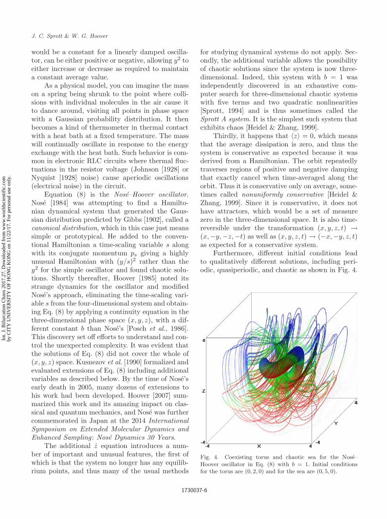
Furthermore, different initial conditions leadto qualitatively different solutions, including peri-odic, quasiperiodic, and chaotic as shown in Fig. 4.

Fig. 4. Coexisting torus and chaotic sea for the Nose–Hoover oscillator in Eq. (8) with b = 1. Initial conditionsfor the torus are (0, 2, 0) and for the sea are (0, 5, 0).

1730037-6

Int.

J. B

ifur

catio

n C

haos

201

7.27

. Dow

nloa

ded

from

ww

w.w

orld

scie

ntif

ic.c

omby

CIT

Y U

NIV

ER

SIT

Y O

F H

ON

G K

ON

G o

n 11

/22/

17. F

or p

erso

nal u

se o

nly.

November 10, 2017 9:10 WSPC/S0218-1274 1730037

Harmonic Oscillators with Nonlinear Damping

The quasiperiodic solution with initial conditions(0, 2, 0) resides on the surface of one of infinitelymany nested tori on the axis of which is a singleperiodic orbit (not shown), and the tori are linkedby a chaotic orbit that forms a chaotic sea, whichis the term used for a chaotic region that is not anattractor.

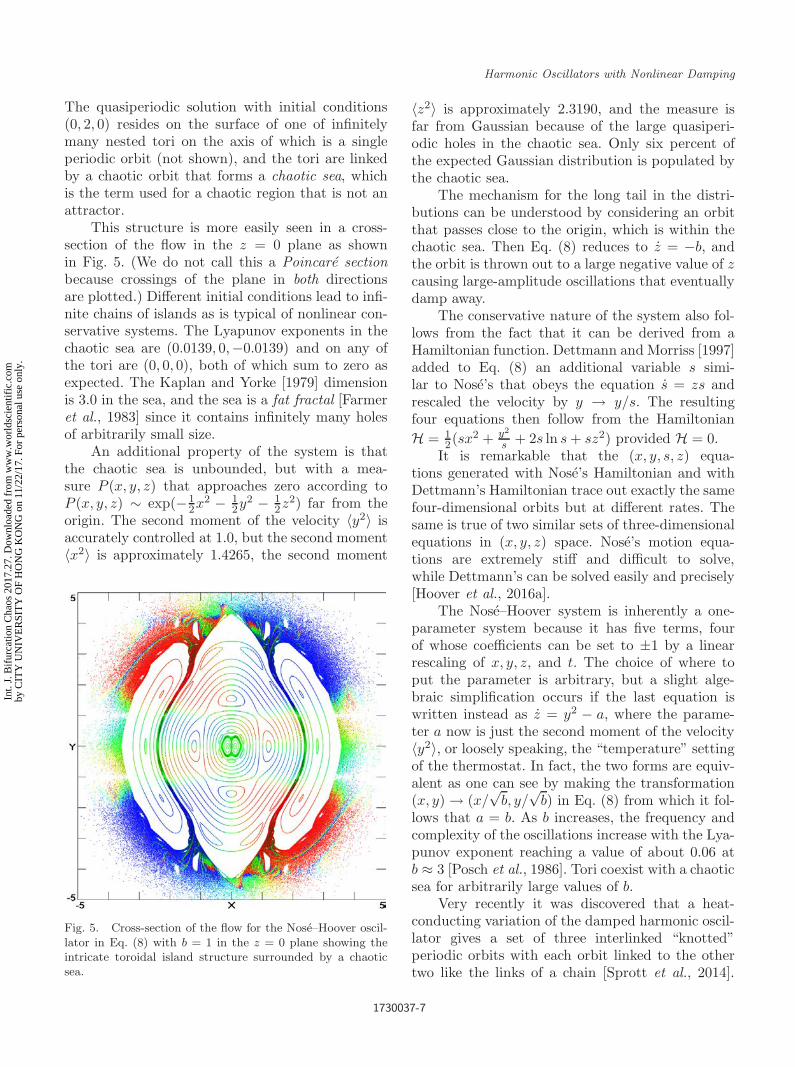
This structure is more easily seen in a cross-section of the flow in the z = 0 plane as shownin Fig. 5. (We do not call this a Poincare sectionbecause crossings of the plane in both directionsare plotted.) Different initial conditions lead to infi-nite chains of islands as is typical of nonlinear con-servative systems. The Lyapunov exponents in thechaotic sea are (0.0139, 0,−0.0139) and on any ofthe tori are (0, 0, 0), both of which sum to zero asexpected. The Kaplan and Yorke [1979] dimensionis 3.0 in the sea, and the sea is a fat fractal [Farmeret al., 1983] since it contains infinitely many holesof arbitrarily small size.

An additional property of the system is thatthe chaotic sea is unbounded, but with a mea-sure P (x, y, z) that approaches zero according toP (x, y, z) ∼ exp(−1

2x2 − 12y2 − 1

2z2) far from theorigin. The second moment of the velocity 〈y2〉 isaccurately controlled at 1.0, but the second moment〈x2〉 is approximately 1.4265, the second moment

Fig. 5. Cross-section of the flow for the Nose–Hoover oscil-lator in Eq. (8) with b = 1 in the z = 0 plane showing theintricate toroidal island structure surrounded by a chaoticsea.

〈z2〉 is approximately 2.3190, and the measure isfar from Gaussian because of the large quasiperi-odic holes in the chaotic sea. Only six percent ofthe expected Gaussian distribution is populated bythe chaotic sea.

The mechanism for the long tail in the distri-butions can be understood by considering an orbitthat passes close to the origin, which is within thechaotic sea. Then Eq. (8) reduces to z = −b, andthe orbit is thrown out to a large negative value of zcausing large-amplitude oscillations that eventuallydamp away.

The conservative nature of the system also fol-lows from the fact that it can be derived from aHamiltonian function. Dettmann and Morriss [1997]added to Eq. (8) an additional variable s simi-lar to Nose’s that obeys the equation s = zs andrescaled the velocity by y → y/s. The resultingfour equations then follow from the HamiltonianH = 1

2(sx2 + y2

s + 2s ln s + sz2) provided H = 0.It is remarkable that the (x, y, s, z) equa-

tions generated with Nose’s Hamiltonian and withDettmann’s Hamiltonian trace out exactly the samefour-dimensional orbits but at different rates. Thesame is true of two similar sets of three-dimensionalequations in (x, y, z) space. Nose’s motion equa-tions are extremely stiff and difficult to solve,while Dettmann’s can be solved easily and precisely[Hoover et al., 2016a].

The Nose–Hoover system is inherently a one-parameter system because it has five terms, fourof whose coefficients can be set to ±1 by a linearrescaling of x, y, z, and t. The choice of where toput the parameter is arbitrary, but a slight alge-braic simplification occurs if the last equation iswritten instead as z = y2 − a, where the parame-ter a now is just the second moment of the velocity〈y2〉, or loosely speaking, the “temperature” settingof the thermostat. In fact, the two forms are equiv-alent as one can see by making the transformation(x, y) → (x/

√b, y/

√b) in Eq. (8) from which it fol-

lows that a = b. As b increases, the frequency andcomplexity of the oscillations increase with the Lya-punov exponent reaching a value of about 0.06 atb ≈ 3 [Posch et al., 1986]. Tori coexist with a chaoticsea for arbitrarily large values of b.

Very recently it was discovered that a heat-conducting variation of the damped harmonic oscil-lator gives a set of three interlinked “knotted”periodic orbits with each orbit linked to the othertwo like the links of a chain [Sprott et al., 2014].

1730037-7

Int.

J. B

ifur

catio

n C

haos

201

7.27

. Dow

nloa

ded

from

ww

w.w

orld

scie

ntif

ic.c

omby

CIT

Y U

NIV

ER

SIT

Y O

F H

ON

G K

ON

G o

n 11

/22/

17. F

or p

erso

nal u

se o

nly.

November 10, 2017 9:10 WSPC/S0218-1274 1730037

J. C. Sprott & W. G. Hoover

Soon after Wang and Yang [2015] explored theNose–Hoover oscillator’s phase space for b = 10.They considered six periodic orbits in (x, y, z) spaceand found that each of them was similarly knottedwith the other five. They also discovered a trefoilknot (an overhand knot in a closed loop). Theseunexpected and unexplained findings invite addi-tional topological studies of the Nose–Hoover oscil-lator’s knot-tying abilities.

3.2. Munmuangsaen oscillator

As a model of a harmonic oscillator driven by ran-dom thermal fluctuations, the Nose–Hoover systemhas a serious flaw in its preponderance of quasiperi-odic solutions. A real physical oscillator would visitall values of (x, y) with a Gaussian probability dis-tribution. The chaotic sea would fill all of spacewithout any holes, and such a system is said tobe ergodic. Starting from any initial condition, theorbit would eventually come arbitrarily close toevery point in the space. A simple system [Mun-muangsaen et al., 2015] that satisfies this conditionfor a = 5 is

x = y,

y = −x − zy,

z = |y| − a.

(9)

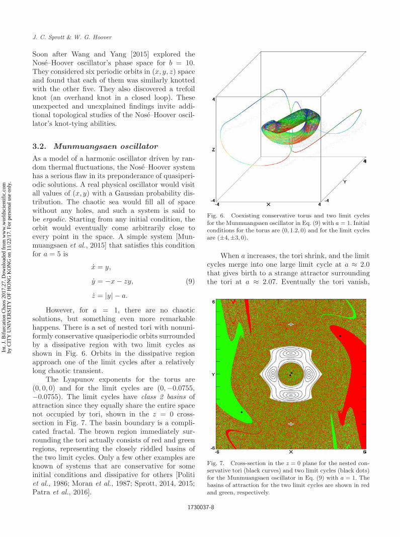
However, for a = 1, there are no chaoticsolutions, but something even more remarkablehappens. There is a set of nested tori with nonuni-formly conservative quasiperiodic orbits surroundedby a dissipative region with two limit cycles asshown in Fig. 6. Orbits in the dissipative regionapproach one of the limit cycles after a relativelylong chaotic transient.

The Lyapunov exponents for the torus are(0, 0, 0) and for the limit cycles are (0,−0.0755,−0.0755). The limit cycles have class 2 basins ofattraction since they equally share the entire spacenot occupied by tori, shown in the z = 0 cross-section in Fig. 7. The basin boundary is a compli-cated fractal. The brown region immediately sur-rounding the tori actually consists of red and greenregions, representing the closely riddled basins ofthe two limit cycles. Only a few other examples areknown of systems that are conservative for someinitial conditions and dissipative for others [Politiet al., 1986; Moran et al., 1987; Sprott, 2014, 2015;Patra et al., 2016].

Fig. 6. Coexisting conservative torus and two limit cyclesfor the Munmuangsaen oscillator in Eq. (9) with a = 1. Initialconditions for the torus are (0, 1.2, 0) and for the limit cyclesare (±4,±3, 0).

When a increases, the tori shrink, and the limitcycles merge into one large limit cycle at a ≈ 2.0that gives birth to a strange attractor surroundingthe tori at a ≈ 2.07. Eventually the tori vanish,

Fig. 7. Cross-section in the z = 0 plane for the nested con-servative tori (black curves) and two limit cycles (black dots)for the Munmuangsaen oscillator in Eq. (9) with a = 1. Thebasins of attraction for the two limit cycles are shown in redand green, respectively.

1730037-8

Int.

J. B

ifur

catio

n C

haos

201

7.27

. Dow

nloa

ded

from

ww

w.w

orld

scie

ntif

ic.c

omby

CIT

Y U

NIV

ER

SIT

Y O

F H

ON

G K

ON

G o

n 11

/22/

17. F

or p

erso

nal u

se o

nly.

November 10, 2017 9:10 WSPC/S0218-1274 1730037

Harmonic Oscillators with Nonlinear Damping

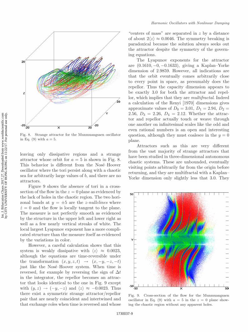
Fig. 8. Strange attractor for the Munmuangsaen oscillatorin Eq. (9) with a = 5.

leaving only dissipative regions and a strangeattractor whose orbit for a = 5 is shown in Fig. 8.This behavior is different from the Nose–Hooveroscillator where the tori persist along with a chaoticsea for arbitrarily large values of b, and there are noattractors.

Figure 9 shows the absence of tori in a cross-section of the flow in the z = 0 plane as evidenced bythe lack of holes in the chaotic region. The two hori-zonal bands at y = ±5 are the z-nullclines wherez = 0 and the flow is locally tangent to the plane.The measure is not perfectly smooth as evidencedby the structure in the upper left and lower right aswell as a few nearly vertical streaks of white. Thelocal largest Lyapunov exponent has a more compli-cated structure than the measure itself as evidencedby the variations in color.

However, a careful calculation shows that thissystem is weakly dissipative with 〈z〉 ≈ 0.0023,although the equations are time-reversible underthe transformation (x, y, z, t) → (x,−y,−z,−t)just like the Nose–Hoover system. When time isreversed, for example by reversing the sign of ∆tin the integrator, the repellor becomes an attrac-tor that looks identical to the one in Fig. 9 exceptwith (y, z) → (−y,−z) and 〈z〉 ≈ −0.0023. Thusthere exist a symmetric strange attractor/repellorpair that are nearly coincident and intertwined andthat exchange roles when time is reversed and whose

“centers of mass” are separated in z by a distanceof about 2〈z〉 ≈ 0.0046. The symmetry breaking isparadoxical because the solution always seeks outthe attractor despite the symmetry of the govern-ing equations.

The Lyapunov exponents for the attractorare (0.1610,−0,−0.1633), giving a Kaplan–Yorkedimension of 2.9859. However, all indications arethat the orbit eventually comes arbitrarily closeto every point in space, as presumably does therepellor. Thus the capacity dimension appears tobe exactly 3.0 for both the attractor and repel-lor, which implies that they are multifractal. Indeeda calculation of the Renyi [1970] dimensions givesapproximate values of D0 = 3.01, D1 = 2.94, D2 =2.56, D3 = 2.26, D4 = 2.12. Whether the attrac-tor and repellor actually touch or weave throughone another on infinitesimal scales like the odd andeven rational numbers is an open and interestingquestion, although they must coalesce in the y = 0plane.

Attractors such as this are very differentfrom the vast majority of strange attractors thathave been studied in three-dimensional autonomouschaotic systems. These are unbounded, eventuallyvisiting points arbitrarily far from the origin beforereturning, and they are multifractal with a Kaplan–Yorke dimension only slightly less that 3.0. They

Fig. 9. Cross-section of the flow for the Munmuangsaenoscillator in Eq. (9) with a = 5 in the z = 0 plane show-ing the chaotic region without any apparent holes.

1730037-9

Int.

J. B

ifur

catio

n C

haos

201

7.27

. Dow

nloa

ded

from

ww

w.w

orld

scie

ntif

ic.c

omby

CIT

Y U

NIV

ER

SIT

Y O

F H

ON

G K

ON

G o

n 11

/22/

17. F

or p

erso

nal u

se o

nly.

November 10, 2017 9:10 WSPC/S0218-1274 1730037

J. C. Sprott & W. G. Hoover

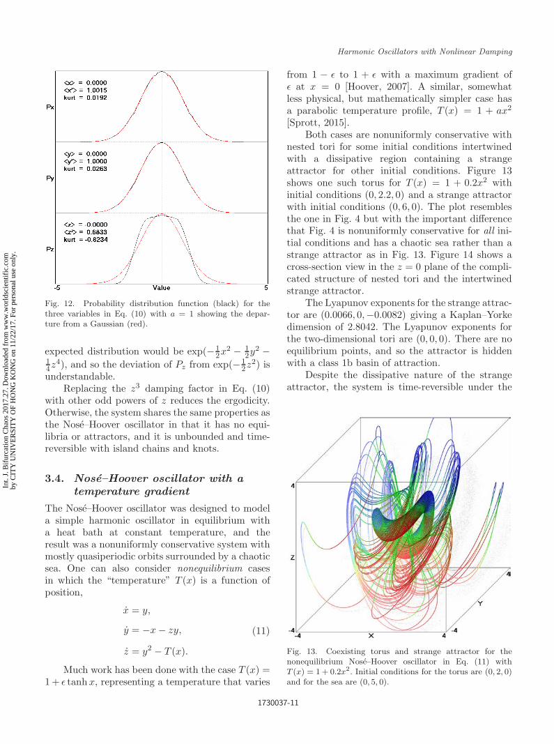
Fig. 10. Probability distribution function for the three vari-ables in Eq. (9) with a = 5 showing the positive kurtosis anddeparture from a Gaussian.

are time-reversible, which is unusual for a dissipa-tive system, and their repellor overlaps and is nearlycoincident with the attractor, both of which fill thewhole of space.

Since there are no equilibria in the system, theattractor is hidden, which is an odd terminologyin this case since the attractor is unbounded andglobally attracting with a class 1a basin (all initialconditions except for a set of measure zero will findthe attractor), and every initial condition is so closeto the attractor that the separation is unobservable.

However, this system is still not a satisfactorymodel of a thermally-excited harmonic oscillatorbecause the measure is not Gaussian. Figure 10shows the probability distribution function for thethree variables. The departure from a Gaussian ismost evident for Py, but all three plots have anonzero kurtosis, which is a measure of the depar-ture of the fourth moment from the expected nor-mal distribution [Press et al., 1992]. The positivekurtosis means the attractor is leptokurtic withenhanced tails relative to a Gaussian.

By adding a −bz term to the z equation inEq. (9), the dimension of the strange attractor canbe continuously and monotonically tuned from 3.0to 2.0 by increasing the value of b for a = 5, andthe predicted behavior has been demonstrated in anelectronic circuit [Munmuangsaen et al., 2015].

3.3. KBB oscillator

In two classic and highly recommended papers,Kusnezov et al. [1990], Kusnezov and Bulgac [1992]describe a general class of thermally-excited oscilla-tors, one especially simple example of which is

x = y,

y = −x − az3y,

z = y2 − a,

(10)

which differs from the Nose–Hoover system only inthe use of z3 rather than z in the damping factor.

A cross-section of the chaotic region in thez = 0 plane for a = 1 is shown in Fig. 11.It is nearly ergodic, but at least twenty smallquasiperiodic holes are evident. Presumably thereare infinitely many ever smaller such holes in a fatfractal distribution. Since the Lyapunov exponentsare (0.0903, 0,−0.0903), the system is nonuniformlyconservative with a Kaplan–Yorke dimension of 3.0and a chaotic sea, but no attractors.

Furthermore, the probability distribution forx and y shown as black curves in Fig. 12 closelyapproximate the Gaussian shown in red, althoughsmall departures are evident, and the distributionis slightly leptokurtic. However, the average 〈y2〉 isaccurately 1.0. Had the system been ergodic, the

Fig. 11. Cross-section of the flow for the KBB oscillator inEq. (10) with a = 1 in the z = 0 plane showing the chaoticsea with at least twenty small quasiperiodic holes.

1730037-10

Int.

J. B

ifur

catio

n C

haos

201

7.27

. Dow

nloa

ded

from

ww

w.w

orld

scie

ntif

ic.c

omby

CIT

Y U

NIV

ER

SIT

Y O

F H

ON

G K

ON

G o

n 11

/22/

17. F

or p

erso

nal u

se o

nly.

November 10, 2017 9:10 WSPC/S0218-1274 1730037

Harmonic Oscillators with Nonlinear Damping

Fig. 12. Probability distribution function (black) for thethree variables in Eq. (10) with a = 1 showing the depar-ture from a Gaussian (red).

expected distribution would be exp(−12x2 − 1

2y2 −14z4), and so the deviation of Pz from exp(−1

2z2) isunderstandable.

Replacing the z3 damping factor in Eq. (10)with other odd powers of z reduces the ergodicity.Otherwise, the system shares the same properties asthe Nose–Hoover oscillator in that it has no equi-libria or attractors, and it is unbounded and time-reversible with island chains and knots.

3.4. Nose–Hoover oscillator with atemperature gradient

The Nose–Hoover oscillator was designed to modela simple harmonic oscillator in equilibrium witha heat bath at constant temperature, and theresult was a nonuniformly conservative system withmostly quasiperiodic orbits surrounded by a chaoticsea. One can also consider nonequilibrium casesin which the “temperature” T (x) is a function ofposition,

x = y,

y = −x − zy,

z = y2 − T (x).

(11)

Much work has been done with the case T (x) =1 + ε tanh x, representing a temperature that varies

from 1 − ε to 1 + ε with a maximum gradient ofε at x = 0 [Hoover, 2007]. A similar, somewhatless physical, but mathematically simpler case hasa parabolic temperature profile, T (x) = 1 + ax2

[Sprott, 2015].Both cases are nonuniformly conservative with

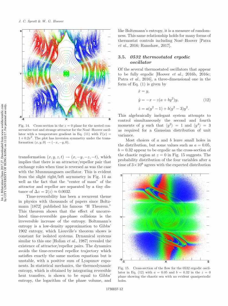
nested tori for some initial conditions intertwinedwith a dissipative region containing a strangeattractor for other initial conditions. Figure 13shows one such torus for T (x) = 1 + 0.2x2 withinitial conditions (0, 2.2, 0) and a strange attractorwith initial conditions (0, 6, 0). The plot resemblesthe one in Fig. 4 but with the important differencethat Fig. 4 is nonuniformly conservative for all ini-tial conditions and has a chaotic sea rather than astrange attractor as in Fig. 13. Figure 14 shows across-section view in the z = 0 plane of the compli-cated structure of nested tori and the intertwinedstrange attractor.

The Lyapunov exponents for the strange attrac-tor are (0.0066, 0,−0.0082) giving a Kaplan–Yorkedimension of 2.8042. The Lyapunov exponents forthe two-dimensional tori are (0, 0, 0). There are noequilibrium points, and so the attractor is hiddenwith a class 1b basin of attraction.

Despite the dissipative nature of the strangeattractor, the system is time-reversible under the

Fig. 13. Coexisting torus and strange attractor for thenonequilibrium Nose–Hoover oscillator in Eq. (11) withT (x) = 1 + 0.2x2. Initial conditions for the torus are (0, 2, 0)and for the sea are (0, 5, 0).

1730037-11

Int.

J. B

ifur

catio

n C

haos

201

7.27

. Dow

nloa

ded

from

ww

w.w

orld

scie

ntif

ic.c

omby

CIT

Y U

NIV

ER

SIT

Y O

F H

ON

G K

ON

G o

n 11

/22/

17. F

or p

erso

nal u

se o

nly.

November 10, 2017 9:10 WSPC/S0218-1274 1730037

J. C. Sprott & W. G. Hoover

Fig. 14. Cross-section in the z = 0 plane for the nested con-servative tori and strange attractor for the Nose–Hoover oscil-lator with a temperature gradient in Eq. (11) with T (x) =1 + 0.2x2. The plot has inversion symmetry under the trans-formation (x, y, 0) → (−x,−y, 0).

transformation (x, y, z, t) → (x,−y,−z,−t), whichimplies that there is an attractor/repellor pair thatexchange roles when time is reversed as was the casewith the Munmuangsaen oscillator. This is evidentfrom the slight right/left asymmetry in Fig. 14 aswell as the fact that the “center of mass” of theattractor and repellor are separated by a tiny dis-tance of ∆z = 2〈z〉 ≈ 0.0032.

Time-reversibility has been a recurrent themein physics with thousands of papers since Boltz-mann [1872] published his famous “H Theorem.”This theorem shows that the effect of uncorre-lated time-reversible gas-phase collisions is theirreversible increase of the entropy. Boltzmann’sentropy is a low-density approximation to Gibbs’1902 entropy, which Liouville’s theorem shows isconstant for isolated systems. Dynamical systemssimilar to this one [Holian et al., 1987] revealed theexistence of attractor/repellor pairs. The dynamicsavoids the time-reversed repellor trajectory whichsatisfies exactly the same motion equations but isunstable, with a positive sum of Lyapunov expo-nents. In statistical mechanics, the thermodynamicentropy, which is obtained by integrating reversibleheat transfers, is shown to be equal to Gibbs’entropy, the logarithm of the phase volume, and

like Boltzmann’s entropy, it is a measure of random-ness. This same relationship holds for many forms ofthermostat controls including Nose–Hoover [Patraet al., 2016; Ramshaw, 2017].

3.5. 0532 thermostated ergodicoscillator

Of the several thermostated oscillators that appearto be fully ergodic [Hoover et al., 2016b, 2016c;Patra et al., 2016], a three-dimensional one in theform of Eq. (1) is given by

x = y,

y = −x − z(a + by2)y,

z = a(y2 − 1) + b(y2 − 3)y2.

(12)

This algebraically inelegant system attempts tocontrol simultaneously the second and fourthmoments of y such that 〈y2〉 = 1 and 〈y4〉 = 3as required for a Gaussian distribution of unitvariance.

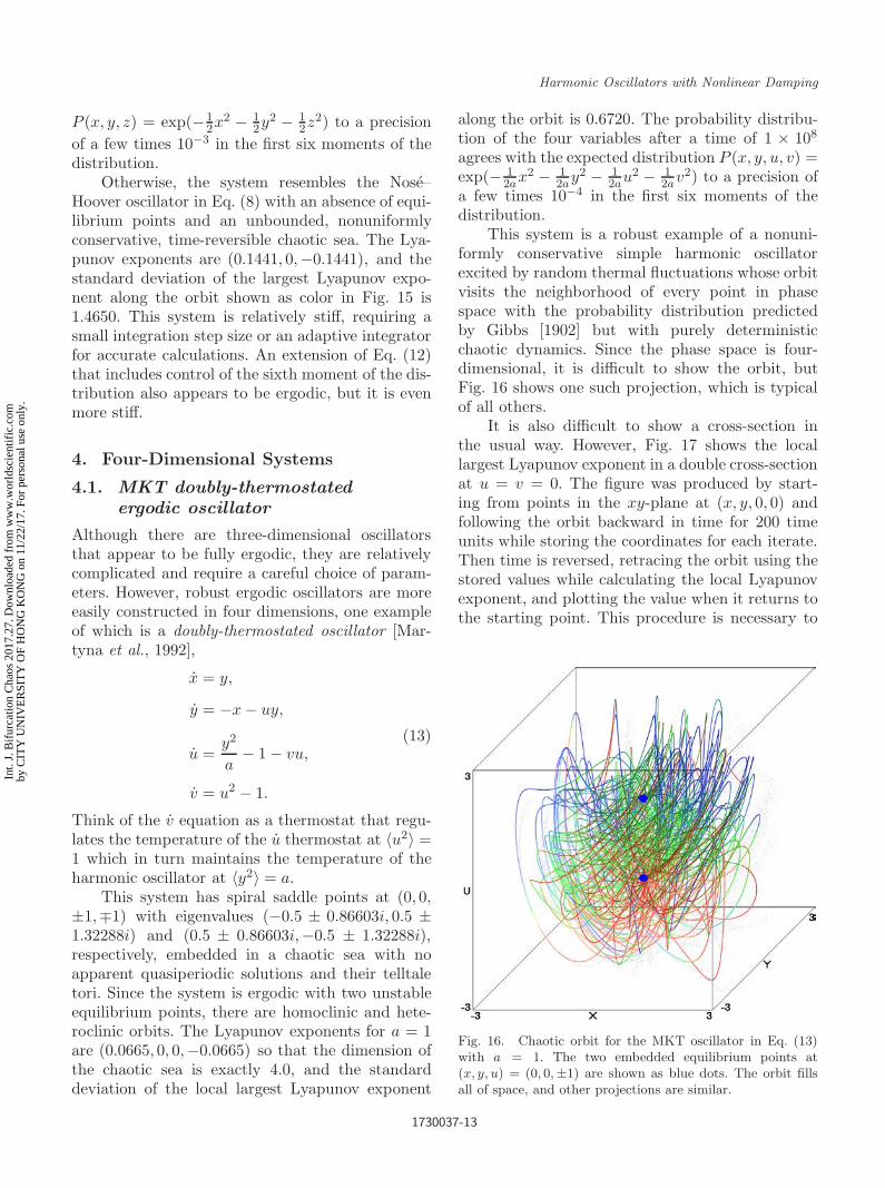
Most choices of a and b leave small holes inthe distribution, but some values such as a = 0.05,b = 0.32 appear to be ergodic as the cross-section ofthe chaotic region at z = 0 in Fig. 15 suggests. Theprobability distribution of the four variables after atime of 3×108 agrees with the expected distribution

Fig. 15. Cross-section of the flow for the 0532 ergodic oscil-lator in Eq. (12) with a = 0.05 and b = 0.32 in the z = 0plane showing the chaotic sea with no evident quasiperiodicholes.

1730037-12

Int.

J. B

ifur

catio

n C

haos

201

7.27

. Dow

nloa

ded

from

ww

w.w

orld

scie

ntif

ic.c

omby

CIT

Y U

NIV

ER

SIT

Y O

F H

ON

G K

ON

G o

n 11

/22/

17. F

or p

erso

nal u

se o

nly.

November 10, 2017 9:10 WSPC/S0218-1274 1730037

Harmonic Oscillators with Nonlinear Damping

P (x, y, z) = exp(−12x2 − 1

2y2 − 12z2) to a precision

of a few times 10−3 in the first six moments of thedistribution.

Otherwise, the system resembles the Nose–Hoover oscillator in Eq. (8) with an absence of equi-librium points and an unbounded, nonuniformlyconservative, time-reversible chaotic sea. The Lya-punov exponents are (0.1441, 0,−0.1441), and thestandard deviation of the largest Lyapunov expo-nent along the orbit shown as color in Fig. 15 is1.4650. This system is relatively stiff, requiring asmall integration step size or an adaptive integratorfor accurate calculations. An extension of Eq. (12)that includes control of the sixth moment of the dis-tribution also appears to be ergodic, but it is evenmore stiff.

4. Four-Dimensional Systems

4.1. MKT doubly-thermostatedergodic oscillator

Although there are three-dimensional oscillatorsthat appear to be fully ergodic, they are relativelycomplicated and require a careful choice of param-eters. However, robust ergodic oscillators are moreeasily constructed in four dimensions, one exampleof which is a doubly-thermostated oscillator [Mar-tyna et al., 1992],

x = y,

y = −x − uy,

u =y2

a− 1 − vu,

v = u2 − 1.

(13)

Think of the v equation as a thermostat that regu-lates the temperature of the u thermostat at 〈u2〉 =1 which in turn maintains the temperature of theharmonic oscillator at 〈y2〉 = a.

This system has spiral saddle points at (0, 0,±1,∓1) with eigenvalues (−0.5 ± 0.86603i, 0.5 ±1.32288i) and (0.5 ± 0.86603i,−0.5 ± 1.32288i),respectively, embedded in a chaotic sea with noapparent quasiperiodic solutions and their telltaletori. Since the system is ergodic with two unstableequilibrium points, there are homoclinic and hete-roclinic orbits. The Lyapunov exponents for a = 1are (0.0665, 0, 0,−0.0665) so that the dimension ofthe chaotic sea is exactly 4.0, and the standarddeviation of the local largest Lyapunov exponent

along the orbit is 0.6720. The probability distribu-tion of the four variables after a time of 1 × 108

agrees with the expected distribution P (x, y, u, v) =exp(− 1

2ax2 − 12ay2 − 1

2au2 − 12av2) to a precision of

a few times 10−4 in the first six moments of thedistribution.

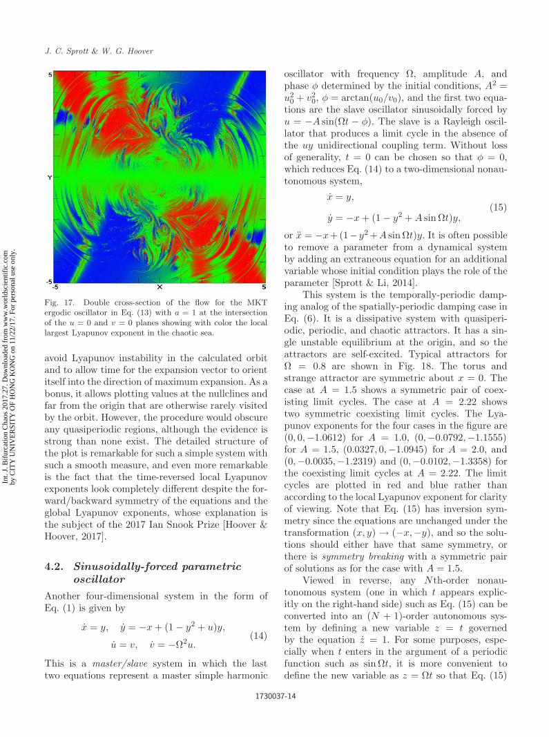
This system is a robust example of a nonuni-formly conservative simple harmonic oscillatorexcited by random thermal fluctuations whose orbitvisits the neighborhood of every point in phasespace with the probability distribution predictedby Gibbs [1902] but with purely deterministicchaotic dynamics. Since the phase space is four-dimensional, it is difficult to show the orbit, butFig. 16 shows one such projection, which is typicalof all others.

It is also difficult to show a cross-section inthe usual way. However, Fig. 17 shows the locallargest Lyapunov exponent in a double cross-sectionat u = v = 0. The figure was produced by start-ing from points in the xy-plane at (x, y, 0, 0) andfollowing the orbit backward in time for 200 timeunits while storing the coordinates for each iterate.Then time is reversed, retracing the orbit using thestored values while calculating the local Lyapunovexponent, and plotting the value when it returns tothe starting point. This procedure is necessary to

Fig. 16. Chaotic orbit for the MKT oscillator in Eq. (13)with a = 1. The two embedded equilibrium points at(x, y, u) = (0, 0,±1) are shown as blue dots. The orbit fillsall of space, and other projections are similar.

1730037-13

Int.

J. B

ifur

catio

n C

haos

201

7.27

. Dow

nloa

ded

from

ww

w.w

orld

scie

ntif

ic.c

omby

CIT

Y U

NIV

ER

SIT

Y O

F H

ON

G K

ON

G o

n 11

/22/

17. F

or p

erso

nal u

se o

nly.

November 10, 2017 9:10 WSPC/S0218-1274 1730037

J. C. Sprott & W. G. Hoover

Fig. 17. Double cross-section of the flow for the MKTergodic oscillator in Eq. (13) with a = 1 at the intersectionof the u = 0 and v = 0 planes showing with color the locallargest Lyapunov exponent in the chaotic sea.

avoid Lyapunov instability in the calculated orbitand to allow time for the expansion vector to orientitself into the direction of maximum expansion. As abonus, it allows plotting values at the nullclines andfar from the origin that are otherwise rarely visitedby the orbit. However, the procedure would obscureany quasiperiodic regions, although the evidence isstrong than none exist. The detailed structure ofthe plot is remarkable for such a simple system withsuch a smooth measure, and even more remarkableis the fact that the time-reversed local Lyapunovexponents look completely different despite the for-ward/backward symmetry of the equations and theglobal Lyapunov exponents, whose explanation isthe subject of the 2017 Ian Snook Prize [Hoover &Hoover, 2017].

4.2. Sinusoidally-forced parametricoscillator

Another four-dimensional system in the form ofEq. (1) is given by

x = y, y = −x + (1 − y2 + u)y,

u = v, v = −Ω2u.(14)

This is a master/slave system in which the lasttwo equations represent a master simple harmonic

oscillator with frequency Ω, amplitude A, andphase φ determined by the initial conditions, A2 =u2

0 + v20, φ = arctan(u0/v0), and the first two equa-

tions are the slave oscillator sinusoidally forced byu = −A sin(Ωt − φ). The slave is a Rayleigh oscil-lator that produces a limit cycle in the absence ofthe uy unidirectional coupling term. Without lossof generality, t = 0 can be chosen so that φ = 0,which reduces Eq. (14) to a two-dimensional nonau-tonomous system,

x = y,

y = −x + (1 − y2 + A sin Ωt)y,(15)

or x = −x+(1−y2 +A sin Ωt)y. It is often possibleto remove a parameter from a dynamical systemby adding an extraneous equation for an additionalvariable whose initial condition plays the role of theparameter [Sprott & Li, 2014].

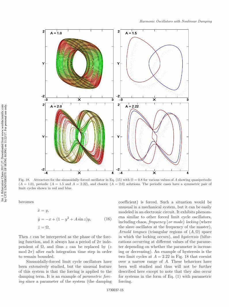
This system is the temporally-periodic damp-ing analog of the spatially-periodic damping case inEq. (6). It is a dissipative system with quasiperi-odic, periodic, and chaotic attractors. It has a sin-gle unstable equilibrium at the origin, and so theattractors are self-excited. Typical attractors forΩ = 0.8 are shown in Fig. 18. The torus andstrange attractor are symmetric about x = 0. Thecase at A = 1.5 shows a symmetric pair of coex-isting limit cycles. The case at A = 2.22 showstwo symmetric coexisting limit cycles. The Lya-punov exponents for the four cases in the figure are(0, 0,−1.0612) for A = 1.0, (0,−0.0792,−1.1555)for A = 1.5, (0.0327, 0,−1.0945) for A = 2.0, and(0,−0.0035,−1.2319) and (0,−0.0102,−1.3358) forthe coexisting limit cycles at A = 2.22. The limitcycles are plotted in red and blue rather thanaccording to the local Lyapunov exponent for clarityof viewing. Note that Eq. (15) has inversion sym-metry since the equations are unchanged under thetransformation (x, y) → (−x,−y), and so the solu-tions should either have that same symmetry, orthere is symmetry breaking with a symmetric pairof solutions as for the case with A = 1.5.

Viewed in reverse, any Nth-order nonau-tonomous system (one in which t appears explic-itly on the right-hand side) such as Eq. (15) can beconverted into an (N + 1)-order autonomous sys-tem by defining a new variable z = t governedby the equation z = 1. For some purposes, espe-cially when t enters in the argument of a periodicfunction such as sin Ωt, it is more convenient todefine the new variable as z = Ωt so that Eq. (15)

1730037-14

Int.

J. B

ifur

catio

n C

haos

201

7.27

. Dow

nloa

ded

from

ww

w.w

orld

scie

ntif

ic.c

omby

CIT

Y U

NIV

ER

SIT

Y O

F H

ON

G K

ON

G o

n 11

/22/

17. F

or p

erso

nal u

se o

nly.

November 10, 2017 9:10 WSPC/S0218-1274 1730037

Harmonic Oscillators with Nonlinear Damping

Fig. 18. Attractors for the sinusoidally-forced oscillator in Eq. (15) with Ω = 0.8 for various values of A showing quasiperiodic(A = 1.0), periodic (A = 1.5 and A = 2.22), and chaotic (A = 2.0) solutions. The periodic cases have a symmetric pair oflimit cycles shown in red and blue.

becomes

x = y,

y = −x + (1 − y2 + A sin z)y,

z = Ω.

(16)

Then z can be interpreted as the phase of the forc-ing function, and it always has a period of 2π inde-pendent of Ω, and thus z can be replaced by (zmod 2π) after each integration time step in orderto remain bounded.

Sinusoidally-forced limit cycle oscillators havebeen extensively studied, but the unusual featureof this system is that the forcing is applied to thedamping term. It is an example of parametric forc-ing since a parameter of the system (the damping

coefficient) is forced. Such a situation would beunusual in a mechanical system, but it can be easilymodeled in an electronic circuit. It exhibits phenom-ena similar to other forced limit cycle oscillators,including chaos, frequency (or mode) locking (wherethe slave oscillates at the frequency of the master),Arnold tongues (triangular regions of (A,Ω) spacein which the locking occurs), and hysteresis (bifur-cations occurring at different values of the parame-ter depending on whether the parameter is increas-ing or decreasing). An example of hysteresis is thetwo limit cycles at A = 2.22 in Fig. 18 that coexistover a narrow range of A. These behaviors havebeen well studied and thus will not be furtherdescribed here except to note that they also occurfor systems in the form of Eq. (1) with parametricforcing.

1730037-15

Int.

J. B

ifur

catio

n C

haos

201

7.27

. Dow

nloa

ded

from

ww

w.w

orld

scie

ntif

ic.c

omby

CIT

Y U

NIV

ER

SIT

Y O

F H

ON

G K

ON

G o

n 11

/22/

17. F

or p

erso

nal u

se o

nly.

November 10, 2017 9:10 WSPC/S0218-1274 1730037

J. C. Sprott & W. G. Hoover

4.3. Symmetricparametrically-coupledoscillators

There is a large literature and considerable currentinterest in systems that involve coupled oscillatorsand their synchronization [Strogatz, 2003]. Manynatural systems such as fireflies, flocking birds, andcircadian rhythms display synchrony, and it wasnoted by Christian Huygens in 1665 that the pen-dulums of two clocks mounted on a wall begin tooscillate together. Perhaps the simplest mathemat-ical example in the form of Eq. (1) that involvestwo identical simple harmonic oscillators coupledthrough their damping terms is

x = y, y = −x − uy,

u = v, v = −u − xv.(17)

One could add a parameter to control the cou-pling strength, but since the individual oscillators

are conservative, it is just as easy to control thecoupling by changing the initial conditions whichchange the amplitude of the oscillation and hencethe strength of the nonlinear coupling.

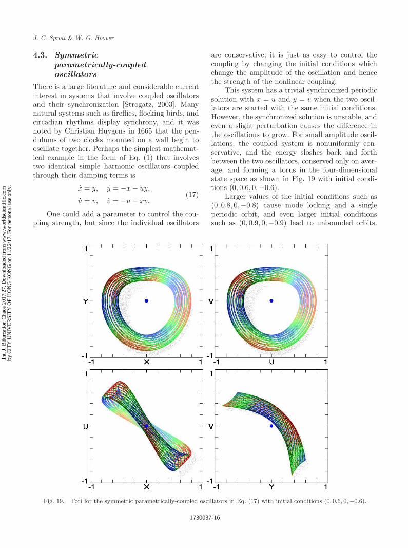
This system has a trivial synchronized periodicsolution with x = u and y = v when the two oscil-lators are started with the same initial conditions.However, the synchronized solution is unstable, andeven a slight perturbation causes the difference inthe oscillations to grow. For small amplitude oscil-lations, the coupled system is nonuniformly con-servative, and the energy sloshes back and forthbetween the two oscillators, conserved only on aver-age, and forming a torus in the four-dimensionalstate space as shown in Fig. 19 with initial condi-tions (0, 0.6, 0,−0.6).

Larger values of the initial conditions such as(0, 0.8, 0,−0.8) cause mode locking and a singleperiodic orbit, and even larger initial conditionssuch as (0, 0.9, 0,−0.9) lead to unbounded orbits.

Fig. 19. Tori for the symmetric parametrically-coupled oscillators in Eq. (17) with initial conditions (0, 0.6, 0,−0.6).

1730037-16

Int.

J. B

ifur

catio

n C

haos

201

7.27

. Dow

nloa

ded

from

ww

w.w

orld

scie

ntif

ic.c

omby

CIT

Y U

NIV

ER

SIT

Y O

F H

ON

G K

ON

G o

n 11

/22/

17. F

or p

erso

nal u

se o

nly.

November 10, 2017 9:10 WSPC/S0218-1274 1730037

Harmonic Oscillators with Nonlinear Damping

This is an example of a system that is (nonuni-formly) conservative for some initial conditions butunbounded for others. Apparently no chaotic solu-tions exist. The equilibrium at the origin has eigen-values (0,±i, 0,±i) and thus is a center for the twooscillators. If either oscillator is started at the ori-gin, it will forever remain there, and the other willoscillate sinusoidally without damping independentof its initial conditions. Altering the frequency ofone of the oscillators can produce long-durationchaotic transients, but apparently not a chaotic sea.

4.4. Asymmetricparametrically-coupledoscillators

To obtain robust chaotic oscillations from two oscil-lators coupled through their damping, it is appar-ently necessary that they have dissipation and dif-ferent natural frequencies. One such example is two

coupled Rayleigh oscillators,

x = y,

y = −x + (1 − y2 + au)y,

u = v,

v = −Ω2u + (1 − v2 + ax)v.

(18)

For a = 0.8 and Ω = 0.8 the strange attrac-tor shown in Fig. 20 results. Initial conditions arenot critical because the attractor has a class 1abasin of attraction, but the regions of parame-ter space that admit chaos are relatively smallwith most solutions periodic or quasiperiodic andbehavior similar to the periodically-forced case inEq. (15). The attractor is self-excited with Lya-punov exponents (0.0146, 0,−0.6236,−2.1699), anda Kaplan–Yorke dimension of 2.0235. The equilib-rium at the origin is an unstable focus with eigen-values (0.5,±0.86603i, 0.5,±0.62450i). The system

Fig. 20. Strange attractor for the asymmetric parametrically-coupled oscillators in Eq. (18) with a = 0.8 and Ω = 0.8.

1730037-17

Int.

J. B

ifur

catio

n C

haos

201

7.27

. Dow

nloa

ded

from

ww

w.w

orld

scie

ntif

ic.c

omby

CIT

Y U

NIV

ER

SIT

Y O

F H

ON

G K

ON

G o

n 11

/22/

17. F

or p

erso

nal u

se o

nly.

November 10, 2017 9:10 WSPC/S0218-1274 1730037

J. C. Sprott & W. G. Hoover

resembles countless others that have been describedin the literature over the past 50 years and thus isunremarkable.

5. Discussion and Conclusions

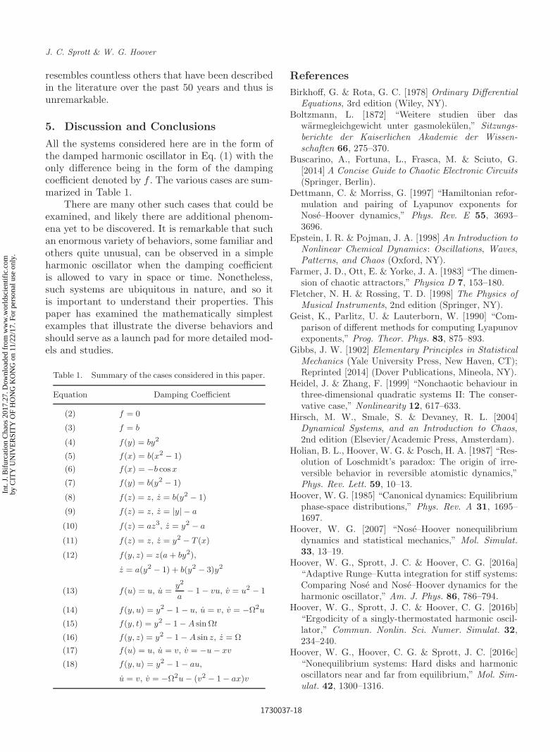
All the systems considered here are in the form ofthe damped harmonic oscillator in Eq. (1) with theonly difference being in the form of the dampingcoefficient denoted by f . The various cases are sum-marized in Table 1.

There are many other such cases that could beexamined, and likely there are additional phenom-ena yet to be discovered. It is remarkable that suchan enormous variety of behaviors, some familiar andothers quite unusual, can be observed in a simpleharmonic oscillator when the damping coefficientis allowed to vary in space or time. Nonetheless,such systems are ubiquitous in nature, and so itis important to understand their properties. Thispaper has examined the mathematically simplestexamples that illustrate the diverse behaviors andshould serve as a launch pad for more detailed mod-els and studies.

Table 1. Summary of the cases considered in this paper.

Equation Damping Coefficient

(2) f = 0

(3) f = b

(4) f(y) = by2

(5) f(x) = b(x2 − 1)

(6) f(x) = −b cos x

(7) f(y) = b(y2 − 1)

(8) f(z) = z, z = b(y2 − 1)

(9) f(z) = z, z = |y| − a

(10) f(z) = az3, z = y2 − a

(11) f(z) = z, z = y2 − T (x)

(12) f(y, z) = z(a + by2),

z = a(y2 − 1) + b(y2 − 3)y2

(13) f(u) = u, u =y2

a− 1 − vu, v = u2 − 1

(14) f(y, u) = y2 − 1 − u, u = v, v = −Ω2u

(15) f(y, t) = y2 − 1 − A sin Ωt

(16) f(y, z) = y2 − 1 − A sin z, z = Ω

(17) f(u) = u, u = v, v = −u − xv

(18) f(y, u) = y2 − 1 − au,

u = v, v = −Ω2u − (v2 − 1 − ax)v

References

Birkhoff, G. & Rota, G. C. [1978] Ordinary DifferentialEquations, 3rd edition (Wiley, NY).

Boltzmann, L. [1872] “Weitere studien uber daswarmegleichgewicht unter gasmolekulen,” Sitzungs-berichte der Kaiserlichen Akademie der Wissen-schaften 66, 275–370.

Buscarino, A., Fortuna, L., Frasca, M. & Sciuto, G.[2014] A Concise Guide to Chaotic Electronic Circuits(Springer, Berlin).

Dettmann, C. & Morriss, G. [1997] “Hamiltonian refor-mulation and pairing of Lyapunov exponents forNose–Hoover dynamics,” Phys. Rev. E 55, 3693–3696.

Epstein, I. R. & Pojman, J. A. [1998] An Introduction toNonlinear Chemical Dynamics : Oscillations, Waves,Patterns, and Chaos (Oxford, NY).

Farmer, J. D., Ott, E. & Yorke, J. A. [1983] “The dimen-sion of chaotic attractors,” Physica D 7, 153–180.

Fletcher, N. H. & Rossing, T. D. [1998] The Physics ofMusical Instruments, 2nd edition (Springer, NY).

Geist, K., Parlitz, U. & Lauterborn, W. [1990] “Com-parison of different methods for computing Lyapunovexponents,” Prog. Theor. Phys. 83, 875–893.

Gibbs, J. W. [1902] Elementary Principles in StatisticalMechanics (Yale University Press, New Haven, CT);Reprinted [2014] (Dover Publications, Mineola, NY).

Heidel, J. & Zhang, F. [1999] “Nonchaotic behaviour inthree-dimensional quadratic systems II: The conser-vative case,” Nonlinearity 12, 617–633.

Hirsch, M. W., Smale, S. & Devaney, R. L. [2004]Dynamical Systems, and an Introduction to Chaos,2nd edition (Elsevier/Academic Press, Amsterdam).

Holian, B. L., Hoover, W. G. & Posch, H. A. [1987] “Res-olution of Loschmidt’s paradox: The origin of irre-versible behavior in reversible atomistic dynamics,”Phys. Rev. Lett. 59, 10–13.

Hoover, W. G. [1985] “Canonical dynamics: Equilibriumphase-space distributions,” Phys. Rev. A 31, 1695–1697.

Hoover, W. G. [2007] “Nose–Hoover nonequilibriumdynamics and statistical mechanics,” Mol. Simulat.33, 13–19.

Hoover, W. G., Sprott, J. C. & Hoover, C. G. [2016a]“Adaptive Runge–Kutta integration for stiff systems:Comparing Nose and Nose–Hoover dynamics for theharmonic oscillator,” Am. J. Phys. 86, 786–794.

Hoover, W. G., Sprott, J. C. & Hoover, C. G. [2016b]“Ergodicity of a singly-thermostated harmonic oscil-lator,” Commun. Nonlin. Sci. Numer. Simulat. 32,234–240.

Hoover, W. G., Hoover, C. G. & Sprott, J. C. [2016c]“Nonequilibrium systems: Hard disks and harmonicoscillators near and far from equilibrium,” Mol. Sim-ulat. 42, 1300–1316.

1730037-18

Int.

J. B

ifur

catio

n C

haos

201

7.27

. Dow

nloa

ded

from

ww

w.w

orld

scie

ntif

ic.c

omby

CIT

Y U

NIV

ER

SIT

Y O

F H

ON

G K

ON

G o

n 11

/22/

17. F

or p

erso

nal u

se o

nly.

November 10, 2017 9:10 WSPC/S0218-1274 1730037

Harmonic Oscillators with Nonlinear Damping

Hoover, W. G. & Hoover, C. G. [2017] “Instantaneouspairing of Lyapunov exponents in chaotic Hamiltoniandynamic and the 2017 Ian Snook prizes,” Comput.Meth. Sci. Technol. 23, 73–79.

Johnson, J. [1928] “Thermal agitation of electricity inconductors,” Phys. Rev. 32, 97–109.

Kahn, P. B. & Zarmi, Y. [1998] Nonlinear Dynamics :Exploration through Normal Forms (Wiley, NY).

Kaplan, J. & Yorke, J. [1979] “Chaotic behavior ofmultidimensional difference equations,” in FunctionalDifferential Equations and Approximation of FixedPoints, Lecture Notes in Mathematics, Vol. 730, eds.Peitgen, H.-O. & Walther, H.-O. (Springer, Berlin,Heidelberg), pp. 477–482.

Krogdahl, W. S. [1955] “Stellar pulsation as a limit-cyclephenomenon,” Astrophys. J. 122, 43–51.

Kusnezov, D., Bulgac, A. & Bauer, W. [1990] “Canonicalensembles from chaos,” Ann. Phys. 204, 155–185.

Kusnezov, D. & Bulgac, A. [1992] “Canonical ensemblesfrom chaos: Constrained dynamical systems,” Ann.Phys. 214, 180–218.

Leonov, G. A. & Kuznetsov, N. V. [2013] “Hidden attrac-tors in dynamical systems. From hidden oscillationin Hilbert–Kolmogorov, Aizerman, and Kalman prob-lems to hidden chaotic attractor in Chua circuits,”Int. J. Bifurcation and Chaos 23, 1330002-1–69.

Martyna, G. J., Klein, M. L. & Tuckerman, M. [1992]“Nose–Hoover chains: The canonical ensemble viacontinuous dynamics,” J. Chem. Phys. 97, 2635–2643.

Mischenko, Y. [2014] “Oscillations in rationaleconomies,” PLoS ONE 9, e87820.

Moran, B., Hoover, W. G. & Bestiale, S. [1987]“Diffusion in a periodic Lorenz gas,” J. Stat. Phys.48, 709–726.

Munmuangsaen, D., Sprott, J. C., Thio, W. J., Bus-carino, A. & Fortuna, L. [2015] “A simple chaotic flowwith a continuously adjustable attractor dimension,”Int. J. Bifurcation and Chaos 25, 1530036-1–12.

Murray, J. D. [1989] Mathematical Biology, 2nd edition(Springer, Berlin).

Nose, S. [1984] “A unified formulation of the constanttemperature molecular dynamics methods,” J. Chem.Phys. 81, 511–519.

Nyquist, H. [1928] “Thermal agitation of electric chargein conductors,” Phys. Rev. 32, 110–113.

Passos, D. & Lopes, I. [2008] “Phase space analysis: Theequilibrium of the solar magnetic cycle,” Solar Phys.250, 403–410.

Patra, P. K., Hoover, W. G., Hoover, C. G. & Sprott,J. C. [2016] “The equivalence of dissipation fromGibbs’ entropy production with phase-volume loss inergodic heat-conducting oscillators,” Int. J. Bifurca-tion and Chaos 26, 1650089-1–11.

Perko, L. [1991] Differential Equations and DynamicalSystems, 3rd edition (Springer, NY), pp. 254–257.

Politi, A., Oppo, G. L. & Badii, R. [1986] “Coexistenceof conservative and dissipative behavior in reversibledynamical systems,” Phys. Rev. A 33, 4055–4060.

Posch, H. A., Hoover, W. G. & Vesely, F. J. [1986]“Canonical dynamics of the Nose oscillator: Stability,order, and chaos,” Phys. Rev. A 33, 4253–4265.

Press, W. H., Flannery, B. P., Teukolsky, S. A. & Vet-terling, W. T. [1992] Numerical Recipes : The Art ofScientific Computing, 2nd edition (Cambridge Uni-versity Press, Cambridge).

Ramshaw, J. D. [2017] “Entropy production and volumecontraction in thermostated Hamiltonian dynamics,”Phys. Rev. E, submitted for publication.

Renyi, A. [1970] Probability Theory (North Holland,Amsterdam).

Sprott, J. C. [1994] “Some simple chaotic flows,” Phys.Rev. E 50, R647–650.

Sprott, J. C. [2014] “A dynamical system with a strangeattractor and invariant tori,” Phys. Lett. A 378,1361–1363.

Sprott, J. C. & Li, C. [2014] “Comment on ‘How toobtain extreme multistability in coupled dynamicalsystems’,” Phys. Rev. E 89, 066901.

Sprott, J. C., Hoover, W. G. & Hoover, C. G. [2014]“Heat conduction, and the lack thereof, in time-reversible dynamical systems: Generalized Nose–Hoover oscillators with a temperature gradient,”Phys. Rev. E 89, 042914.

Sprott, J. C. [2015] “Strange attractors with variousequilibrium types,” Eur. Phys. J. Special Topics 224,1409–1419.

Sprott, J. C. & Xiong, A. [2015] “Classifying and quan-tifying basins of attraction,” Chaos 25, 083101.

Sprott, J. C., Jafari, S., Khalaf, A. J. M. & Kapita-niak, T. [2017] “Megastability: Coexistence of a count-able infinity of nested attractors in a periodically-forced oscillator with spatially-periodic damping,”Eur. Phys. J. Special Topics 226, 1979–1985.

Strogatz, S. H. [2003] Sync (Hyperion, NY).van der Pol, B. [1920] “A theory of the amplitude of free

and forced triode vibrations,” Radio Rev. 1, 701–710,754–762.

van der Pol, B. [1926] “On relaxation oscillations,” Phil.Mag. Ser. 7 2, 978–992.

van der Pol, B. & van der Mark, J. [1928] “The heart-beat considered as a relaxation oscillation, and theelectrical model of the heart,” Phil. Mag. Ser. 7 6,763–775.

Wang, L. & Yang, X. [2015] “The invariant tori of knottype and the interlinked invariant tori in the Nose–Hoover oscillator,” Eur. Phys. J. B 88, 78.

Wolf, A., Swift, J. B., Swinney, H. L. & Vastano, J. A.[1985] “Determining Lyapunov exponents from a timeseries,” Phys. Nonlin. Phenom. 16, 285–317.

1730037-19

Int.

J. B

ifur

catio

n C

haos

201

7.27

. Dow

nloa

ded

from

ww

w.w

orld

scie

ntif

ic.c

omby

CIT

Y U

NIV

ER

SIT

Y O

F H

ON

G K

ON

G o

n 11

/22/

17. F

or p

erso

nal u

se o

nly.