Harmonization of a multi-sensor navigation system

Eric Dorveaux and Nicolas PetitMINES-ParisTech / Département Mathématiques et Systèmes / Centre Automatique et Systèmes (CAS), Paris, France.

Email: {eric.dorveaux | nicolas.petit}@mines-paristech.fr

Abstract—We address the problem of harmonization of twosubsystems used separately to measure a velocity in a bodyreference frame and an attitude with respect to an inertialframe. This general problem is of particular importance whenthe two subsystems are jointly used to obtain an estimate of theinertial velocity, and, then, the position through an integrationprocedure. Typical possible applications encompass pedestriannavigation, and, more generally, indoor navigation. The paperdemonstrates how harmonization can be achieved thanks toan analysis of propagation of projection errors. In particular,trajectories known to be closed can be used to determineone dominant harmonization factor which is the pitch relativeorientation angle between the two subsystems. Computationsyielding the harmonization procedure are exposed in this article,and experimental data serve to illustrate the application of theproposed method.

Keywords—Indoor Positioning, Harmonization, Calibration,Path Reconstruction, Inertial Sensor.

INTRODUCTION

Recently, numerous multi-sensors systems for indoor nav-

igation have been proposed. Among the currently studied

technologies, several rely on radio signals from preinstalled

infrastructures like iGPS, WLan, Wifi and Ultra Wide Band

(UWB), and some others rely on various kinds of beacon,

like ultra sounds systems or fingerprinting techniques. Alter-

natively, infrastructure-free techniques are also studied, like

vision-based systems or systems using inertial navigation such

as foot-mounted inertial measurement unit (IMU). Several

of these technologies are often combined. The benefits of

simultaneously using multiple sensors are essentially two-

folds: i) various type of information can be obtained, ii) the

overall robustness of the information obtained through data

reconciliation is largely improved. While being practically

very effective, these techniques also have flaws. A key aspect

of these complex embedded systems is that information from

the various sources must be harmonized, i.e. some procedure

is necessary to make the informations consistent. While of

importance, this aspect is often underestimated, even by

practitioners. We address it in this paper.

Among the sources of inconsistencies between the sensors

are individual sensor ill-calibration, and relative misalign-

ments of their frames of references. Individually, each sensor

has its own defects. Fortunately, numerous methods can be

used to calibrate them. These methods are usually sufficient to

determine scale factors and biases ([1], [2], [6], [8]). For this

reason, in this paper, we assume that the sensors themselves

are already calibrated and we consider the problem of sensors

harmonization.

The setup we consider in this study is a positioning system

consisting of an inertial velocity estimator whose output signal

is integrated over time. Two sources of information are used

to obtain this estimate: a body velocity estimate and an

978-1-4577-1804-5/11/$26.00 c©2011 IEEE

attitude sensor. This set-up covers a large class of navigation

systems. A first example is a velocimeter and a compass

used to estimate the position of a wheeled robot (e.g. Pioneer

IV Mobile Robots). A second example is a visual (camera-

based) odometer used in conjunction with an IMU for attitude

estimate ([5], [7]). A third application is a body mounted laser

or Doppler radar used with an IMU attitude sensor ([4]). From

a theoretical viewpoint, such systems use an estimate of the

body velocity, expressed in the reference frame of the sensors

providing this information, and an attitude estimate, expressed

in the reference frame of the IMU. Assuming that all the

sensors are attached to a common rigid body, there exists

a constant rotation matrix (referred to as the harmonizationmatrix in this article) between the two considered frames of

reference. In general, this matrix is not the identity matrix, and

when it is ignored when determining a velocity with respect to

the inertial frame of reference, the process results in projection

errors. As the errors are integrated over time, the reconstructed

trajectories drift.

The paper proposes a method to compensate for such

drift. Notations and the problem statement are presented in

Section I. In Section II, an analytic study exposes the sources

of the problem, and shows that the harmonization matrix

can be identified by a simple experimental procedure. The

discussed pedestrian application is considered for sake of

illustration. The main result shows that the dominant terms in

the harmonization matrix (the pitch angle) can be determined

by analysis of the vertical drift observed along a closed

curve. Experimentally, this result can be very conveniently

exploited in an on-the-field calibration procedure, where the

user carrying the considered positioning system is simply

asked to walk along a closed curve of his choice. At his return

point, the harmonization matrix is automatically calculated,

which permits to calibrate the multi-sensor system. These

practical topics are presented in Section III. Finally some

experimental results are presented in Section IV.

I. PROBLEM STATEMENT & NOTATIONS

The problem we wish to address is to estimate the harmo-

nization matrix (totally or at least its most impacting terms)

between the frame where the velocity is measured or estimated

and the one in which the attitude is known.

Consider the following systems, each being attached to a

coordinate frame:

• a building considered as the inertial frame of reference

�I (with its horizontal plane denoted x-y and z pointing

upward);

• a pedestrian moving in the building with an attached

frame �ped whose x and y-axis are horizontal and x is

pointing forward;

• a subsystem providing an inertial speed expressed in its

own coordinate frame �vel;

• an IMU providing the attitude of its own coordinate

frame �IMU with respect to the inertial frame of refer-

ence �I . The attitude is initialized such that the gravity

is on the vertical axis 1.

Indices ped, vel, IMU and I refer to which frame the

corresponding quantity is expressed in. For instance, Vvelis the speed expressed in �vel, whereas VIMU is the same

speed expressed in �IMU . Figure 1 pictures the introduced

coordinate frames and indicates the rotation matrices between

them. The ones of interest are:

• Rplane = Rped→I , rotation matrix from the pedestrian

frame to the inertial frame (unknown)

• RTbody = Rped→vel, rotation matrix from the pedestrian

frame to the velocity sensor frame (unknown)

• Rharmo = Rvel→IMU , rotation matrix from the velocity

sensor frame to the IMU frame (unknown, to be identi-

fied)

• Ratt = RIMU→I , rotation matrix from the IMU frame

to the inertial frame (measured by the IMU).

PedestrianRped

Rbody(unknown)

Vvel( d)

Velocity sensorRvel

Rped(unknown)(measured)

Rvel

Rharmo

Inertial measurement Unit

(unknown)

Inertial measurement UnitRIMU

Rplane(unknown)

••Ratt(measured)

Building (inertial)RI

Fig. 1. Diagram representing the various coordinate frames and rotationmatrices of interest. The speed Vvel is measured in the velocity frame �vel.The rotation matrix RIMU→I = Ratt is measured. The rotation matrixRharmo is to be identified.

The following useful relations hold

VI = RattRharmo Vvel︸︷︷︸speed which is measured

(1)

Vvel = RTbodyVped

and I3 = RattRharmoRTbodyR

Tplan

which yields VI = RplanRbodyVvel (2)

The most interesting frame to express the speed in is the

inertial frame �I . Indeed, in this frame, it is possible to

integrate it to obtain the trajectory of the pedestrian in the

building. However, the speed is measured in the velocity frame

�vel. The matrix Rbody is unknown and is relatively uncertain

because, each time the pedestrian uses the navigation system,

it could be put into a slightly different orientation. Finally,

Rplane is unknown as well. Therefore, the easiest way to

express the speed in the inertial frame is to determine the

1 The yaw angle is left free to allow a later absolute alignment (e.g. usinga map if one is available).

harmonization matrix Rharmo between the velocity frame

and the IMU-frame, and thus exploit Equation (1) and not

Equation (2). This matrix depends only on the relative ori-

entations of the two sensor subsystems. The positions and

orientations of the subsystems being constant, Rharmo needs

to be identified only once and for all.

The relative position at any current time T , P (T )− P (0),with respect to an inertial position P (0) is given through

P (T ) = P (0) +

∫ T

0

RattRharmoVveldt (3)

Ideally, the harmonization matrix Rharmo should be close to

identity, but errors of a few degrees cannot be avoided in the

actual set-up of the subsystems when off-the-shelf packaged

sensors are used. In the following, we model the impact on

trajectory reconstruction when this matrix is omitted. Then,

we show how to compensate for this error.

II. IDENTIFICATION AND CORRECTION OF TRAJECTORY

ERRORS DUE TO AN HARMONIZATION ERROR

A. Trajectory errors: the shape of the trajectory is altered

For sake of illustration, we consider a particular case where

the pedestrian is walking with a speed of constant norm, and,

for simplicity, in the forward direction (i.e. along the x-axis of

�ped). First, we assume that the pedestrian frame, the velocity

frame and the IMU frame are identical, i.e. that Rharmo =Rbody = I3. So, we have

Vped = Vvel = VIMU =

⎛⎝V00

0

⎞⎠

Further, we assume that the pedestrian is walking in an

horizontal plane over the time interval [0, T ]. The IMU

attitude is thus expressed using a single angle α(t)

Ratt(t) =

⎛⎝cos(α) − sin(α) 0sin(α) cos(α) 0

0 0 1

⎞⎠ = R (α(t)) (4)

Through Equation (3), one gets

P (T ) =P (0) +

∫ T

0

R(α(t)) · VIMU · dt

=P (0) + V0

∫ T

0

⎛⎝cos(α)sin(α)

0

⎞⎠ · dt

Now, assume that the pedestrian has walked along a closed-

curve. Then, P (T ) = P (0). From the previous equality, we

deduce that 2.∫ T

0

cos(α(t))dt =

∫ T

0

sin(α(t))dt = 0 (5)

Now, we introduce an harmonization error, i.e. there is

now a rotation Rharmo �= I3 between the coordinate frame

where the speed is measured in (�vel) and the one where

the attitude is measured in (�IMU ). We split up Rharmo into

2One shall note that this last property is true even if the velocity VIMU isnot aligned with the x-axis but belongs to the x− y plane (see Section III).

three successive canonical constant rotations (roll φ, pitch θ,

and yaw ψ in this order from �IMU to �vel) and note RTharmo⎛

⎝c(ψ) −s(ψ) 0s(ψ) c(ψ) 00 0 1

⎞⎠

⎛⎝ c(θ) 0 s(θ)

0 1 0−s(θ) 0 c(θ)

⎞⎠

⎛⎝1 0 00 c(φ) −s(φ)0 sφ) c(φ)

⎞⎠

Assume that the velocity frame �vel has been slightly

rotated. The speed VIMU =(V0 0 0

)Tin the IMU-frame

is unchanged, but the speed measured in the velocity frame

�vel now writes

Vvel =RTharmo

⎛⎝V00

0

⎞⎠

=V0

⎛⎝c(θ) · c(ψ)c(θ) · s(ψ)

−s(θ)

⎞⎠

�=VIMU

If the harmonization error is not taken into account in the

trajectory reconstruction, one obtains

Pr(T )− P (0) =∫ T

0

Ratt(t)Vvel · dt (6)

= V0 ·∫ T

0

⎛⎝c(α(t)) −s(α(t)) 0s(α(t)) c(α(t)) 0

0 0 1

⎞⎠

⎛⎝c(θ) · c(ψ)c(θ) · s(ψ)

−s(θ)

⎞⎠ · dt

=

⎛⎝ 0

0−T · V0 · sin(θ)

⎞⎠T

�= 0 = P (T )− P (0) (7)

where the vector(c(θ) · c(ψ) c(θ) · s(ψ) −s(θ))T has

been put outside the integral since it is constant.

According to Equation (7), the reconstructed position will

then slightly, but constantly, drift downward (or upward

depending on the signs of θ and V0) as illustrated in the

simulation presented in Figure 2. In Figure 3, the same

drift can be observed on experimental data obtained with the

system briefly presented in Section IV. As a consequence,

even if closed paths are followed, the estimated trajectory will

not go back to the starting point as it should. Interestingly,

one can note that the two other angles have no impact on

Equation (7). Only the pitch angle θ alters the shape of the

reconstructed trajectory. The trajectory will simply be rotated

if the yaw angle is not zero (as illustrated in Figure 2 when

only the pitch angle is corrected). The roll angle does not have

any effect since the movement is performed along its rotation

axis. Note that the error in Equation (7) is proportional to the

traveled distance V0 ·T . An angle as small as 3 degrees leads

to an error of more than 5% of the traveled distance.

B. First proposed calibration procedure

In Section II-A, we have explained how even a small

pitch angle error could alter the shape of the trajectory at

a macroscopic scale. A first calibration procedure is proposed

in this section. It takes advantage of this property. From

the measurements, both the traveled distance V0 · T and the

reconstructed trajectory neglecting the harmonization matrix

(Equation (6)) are easily computable. They lead to the fol-

lowing simple calibration procedure:

1) Walk along any closed-loop trajectory in the horizontal

plane with the following constraints: the speed direction

0

0.5

1

1.5

0

0.5

1

1.5

-1.5

-1

-0.5

0

X (m)Y (m)

5 small laps (start in (0,0,0))

Z (

m)

Actual trajectoryNaively reconstructed trajectoryPitch-corrected reconstructed trajectory

Theoretical harmonization roll: 0.07 rdpitch: 0.05 rdyaw: 0.07 rd

Fig. 2. Simulation results - The harmonization angles are given on the rightof the figure. Neglecting the harmonization, even for low pitch angles, cangenerate important drifts. Performing the harmonization with only a pitch-angle eliminates the closure error.

Fig. 3. Experimental results - Many laps (each being about 90 m long) areperformed in the same loop-shaped corridor during about 45 minutes, for atotal length of 3 km. The drift, due to the altitude deviation being projected,is clearly visible.

must be kept along the x-axis of the IMU, the velocity

should be constant, and the IMU must be kept horizontal

(i.e. its z-axis should be kept vertical).

2) Compute the naively reconstructed trajectory according

to Equation (6) recalled below. Note Pr(T ) the final

point.

Pr(T )− P (0) =∫ T

0

Ratt(t)Vvel · dt (6)

3) Identify the pitch angle θ thanks to Equation (7).

sin(θ) = ‖Pr(T )− P (0)‖ · −1V0 · T (8)

This calibration procedure identifies the incriminated angle

rather straightforward. Some of the constraints may seem hard

to fulfill. However, most of them will be relaxed in Section III.

III. PRACTICAL CALIBRATION RESULTS AND LIMITATIONS

A. Further theoretical investigations

The example of Section II shows a particular case where a

single angle is responsible for the non-closing of the recon-

structed trajectory. We now present another viewpoint which

will allow us to take some further errors in the trajectory

reconstruction into account, and remove some constraints

from the proposed calibration procedure. We assume that

the pedestrian is performing a closed-loop trajectory with

the time-varying speed in a constant direction in its own

frame �ped (forward for instance, as in Section II). The speed

direction is then constant in the three frames �ped, �vel,

and �IMU (but the speed directions do not have the same

expressions in the three frames).

Again, from Equation (3), we have

P (T )− P (0) =∫ T

0

Ratt(t)RharmoVvel(t)dt

The speed direction being constant in the velocity frame,

it can be put outside the integral sign, allowing to put the

constant matrix Rharmo outside the integral sign too. DenoteVvel

‖Vvel‖ the constant speed direction in the velocity frame, and

vvel(t) = ‖Vvel(t)‖ its magnitude. Then, one gets

P (T )− P (0) =∫ T

t0

vvel(t)Ratt(t)dt︸ ︷︷ ︸M

RharmoVvel‖Vvel‖ (9)

If the path followed by the pedestrian is a closed-loop trajec-

tory, P (T ) = P (0), which means that M has not full rank

and Rharmo must send Vvel

‖Vvel‖ in the kernel of M . Further,

M has the following property.

Proposition 1: Consider a plane closed trajectory followed

with a constant speed direction in the �ped frame of reference

(without spinning around that direction), starting at time t=0

and ending at time t=T. Denote the speed magnitude

vvel(t) = vIMU (t) = ‖Vvel(t)‖Then, the 3x3 matrix

M =

∫ T

0

vIMU (t)Ratt(t)dt

has rank 1, and its only non-zero singular value is the traveled

distance.

The proof is given in Appendix A. According to Equa-

tion (9), to close the reconstructed trajectory, and thus correct

the pitch angle discussed in Section II, one simply has to

find an harmonization matrix that sends Vvel

‖Vvel‖ in the vector

space of the null singular value of M . For instance, a rotation

matrix that sends Vvel

‖Vvel‖ on the direction of its projection on

the plane of null singular value is a solution 3.

B. Dealing with experimental data

In practice, the actual attitude and the actual velocity

are almost never known, but estimated. Information about

those quantities is provided through sensors, either directly

or, more often, through data filtering. Denote by index f

3Note that this plane corresponds to the degree of freedom left by the yawangle ψ in Section II.

the corresponding filtered quantities that are available. By

integration, one gets the reconstructed position Pr(t)

Pr(T )− P (0) =∫ T

0

vfvel(t)Rfatt(t)dt︸ ︷︷ ︸

Mf

RharmoV fvel∥∥∥V fvel

∥∥∥As stated in Proposition 1, M has a plane of null singular

values and its only non-zero singular value is the traveled

distance. Due to the limited bandwidth of the sensors and the

filters, Mf does not have a plane of perfectly null singular

value. As a consequence, the reconstructed trajectory cannot

be made perfectly closed thanks to an harmonization matrix.

However, Mf is not very different from M . Experiments

show that the singular values of Mf are close to those of M :

two are close to zero (almost identical), and a third one is close

to the traveled distance. The closure error can be minimized

by choosing an Rharmo sendingV fvel

‖V fvel‖ in the vector space

of the two smallest singular values. If the speed direction has

been kept perfectly constant in the pedestrian frame �ped, the

smallest singular value is indeed the lowest closure error that

can be achieved by choosing Rharmo. Experimental results

are provided in Section IV.

C. Second proposed calibration procedure

A first calibration procedure has been proposed in Sec-

tion II-B. Some constraints, potentially hard to fulfill without

dedicated equipment were required to perform that procedure.

The approach presented in Section III allows to remove or

weaken most of them in a new calibration procedure. We now

present this procedure.

1) Walk along any closed-loop trajectory in the horizontal

plane with the following constraint: the speed direction

must be kept along the x-axis of the IMU.

2) Compute the matrix

Mf =

∫ T

0

vfvel(t)Rfatt(t)dt (10)

3) Identify the plane of smaller singular values of Mf

(supposed to be identical).

4) Find a rotation matrix Rharmo which sends the speed

direction Vd =V fvel

‖V fvel‖ to its projection P (Vd) =

P

(V fvel

‖V fvel‖

)/

∥∥∥∥ V fvel

‖V fvel‖

∥∥∥∥ in that plane of singular values,

for instance thanks to Olinde Rodrigues’ formula.

N =P (Vd)× Vd‖P (Vd)× Vd‖ =

⎛⎝N1

N2

N3

⎞⎠ (11)

α =acos(V Td P (Vd)

)(12)

Rharmo =cos(α)I3 + (1− cos(α))NNT (13)

+ sin(α)

⎛⎝ 0 −N3 N2

N3 0 −N1

−N2 N1 0

⎞⎠ (14)

Two of the requirements of the first calibration procedure

have been removed: keeping the speed constant and the z-

axis vertical. The required trajectory is now simply the one

naturally performed by any pedestrian walking, for instance,

in a loop-shaped corridor. This allows the system to be

calibrated very easily in the field by any operator.

-20

-10

0

-20

-10

0-0.50.5

X (m)

Pitch-corrected Reconstruction

Y (m)

Z (

m)

-20

-10

0

-20

-10

0-4

0

X (m)

Raw data integration

Y (m)

Z (

m)

Traveled distance: 165mFinal corrected "closure error": 1.79mFinal raw "closure error": 3mAltitude variation (corrected): <1mAltitude variation (raw): 3.5mPitch angle determined: 0.8°

3D Indoor Trajectory2 laps in an office building

Fig. 4. Experimental data - The pitch-angle has been corrected. The trajectory does not drift downward anymore.

IV. EXPERIMENTAL VALIDATION

In order to evaluate the proposed calibration method, a

system following the modular design in two separate modules

for speed and attitude estimations has been implemented. The

attitude is classically estimated by use of inertial sensors

(see [3], and the references therein) while the velocity estimate

is provided through a set of spatially distributed magnetome-

ters as proposed in [9]. Briefly, the magnetic field dynamics

in the velocity frame writes

˙Mvel = −Ω×Mvel + Jvel(M)Vvel (15)

where Mvel denotes the magnetic field in the velocity frame.

It is measured by the magnetometers. Ω, the rate of turn

between the velocity frame and the inertial frame of reference

�I , is given by a gyrometer. Jvel(M) denotes the Jacobian

of the magnetic field expressed in the velocity frame, i.e. it

represents the local spatial variations of the magnetic field. It

is obtained from the measurements of the spatially distributed

magnetometers set through a simple finite difference scheme.

Finally, Vvel is the sought after velocity. Thus, the measure-

ment system consists of a set of distributed magnetometers

and an IMU. Both of them are attached to a single rigid

board. This board is carried by the pedestrian whose trajectory

is reconstructed. The system is detailed on Figure 5, and

illustrated in Figure 6, where it is carried by a pedestrian.

Fig. 5. The experimental system consists of an inertial measurement unitto estimate the attitude, and of a set of spatially distributed magnetometersto separately estimate the velocity.

Fig. 6. The experimental system in action.

Figure 4 shows some detailed experimental results. The

trajectory is reconstructed after walking two laps along a loop-

shaped corridor in an office building with the described pedes-

trian navigation system in the back. The red curve represents

the (raw) trajectory obtained without taking the harmonization

matrix into account, whereas the blue one is obtained from

the same data but with insertion of the harmonization matrix

(the pitch rotation angle is about 0.8 degrees). The altitude

drift is canceled.

Finally, we show, in Figure 7, an example of reconstructed

trajectory that can be achieved by the system once the harmo-

nization matrix has been found. The trajectory is projected on

a 2-D map of the building. After a 220 m walk in two levels of

an office building, the final error is approximatively 5 m. (The

typical error of this system is about 4 − 5% of the traveled

distance.)

V. CONCLUSION AND FUTURE WORK

In this paper, the harmonization errors between a velocime-

ter and an attitude sensor mounted on the same rigid body has

been analyzed. It has been shown that a single pitch angle

harmonization error is responsible for altering the shape of

the reconstructed trajectory, e.g. by making a closed trajectory

opened. A simple procedure to estimate this angle has been

Position (in m)

X

Y

-50 -40 -30 -20 -10 0 10

-25

-20

-15

-10

-5

0

5

Fig. 7. Example of reconstructed trajectory. The pedestrian starts at the entrance of the building after passing the doors, walks through the huge hall, walkthe stairs one level up. Then, he takes a bridge over the hall, go along the offices, takes another bridge over the hall, goes down the steps, and goes back toits starting point. The final error is about 5 meters after walking 220 m in 4 minutes and 19 seconds.

proposed, which can easily be performed on the field. Then,

a more general formulation being able to account for some

further imperfections due to the filtering of measurements

has been proposed. Further developments will include the

identification of less detrimental effects on the orientation of

the trajectory.

ACKNOWLEDGMENTS

This work was partially funded by the SYSTEM@TIC

PARIS-REGION Cluster in the frame of project LOCIN-

DOOR.

REFERENCES

[1] S. Esquivel, F. Woelk, and R. Koch. Calibration of a multi-camerarig from non-overlapping views. Lecture Notes in Computer Science(including subseries Lecture Notes in Artificial Intelligence and LectureNotes in Bioinformatics), 4713 LNCS:82–91, 2007.

[2] D. Gebre-Egziabher, G. Elkaim, J. Powell, and B. Parkinson. A non-linear, two-step estimation algorithm for calibrating solid-state strapdownmagnetometers. In 8th International St. Petersburg Conference onNavigation Systems (IEEE/AIAA), May 2001.

[3] T. Hamel and R. Mahony. Image based visual servo-control for a classof aerial robotic systems. Automatica, 43(11):1975–1983, 2007.

[4] J. Hesch, F. Mirzaei, G. Mariottini, and S. Roumeliotis. A laser-aidedinertial navigation system (l-ins) for human localization in unknownindoor environments. In Proc. of the 2010 IEEE International Conferenceon Robotics and Automation (ICRA), pages 5376–5382, 2010.

[5] F. Mirzaei and S. Roumeliotis. A kalman filter-based algorithm for imu-camera calibration: Observability analysis and performance evaluation.IEEE Transactions on Robotics, 24(5):1143–1156, 2008.

[6] M. A. Penna. Camera calibration: A quick and easy way to determinethe scale factor. IEEE Transactions on Pattern Analysis and MachineIntelligence, 13(12):1240–1245, 1991.

[7] C. Taylor. Long-term accuracy of camera and imu fusion-based navi-gation systems. In Proc. of the Conference of Institute of Navigation- International Technical Meeting, ITM 2009, volume 1, pages 93–101,2009.

[8] R. Tillett. A calibration system for vision-guided agricultural robots.Journal of Agricultural Engineering Research, 42(4):267–273, 1989.

[9] D. Vissière, A.-P. Martin, and N. Petit. Using spatially distributedmagnetometers to increase IMU-based velocity estimation in perturbedareas. In Proc. of the 46th IEEE Conf. on Decision and Control, 2007.

APPENDIX A

Proof: First assume that the IMU has its x and y axis in

the horizontal plane. The attitude is then a simple rotation

around the vertical z axis defined by a single angle α(t)as already defined in Equation (4). For any constant speed

direction

VIMU

‖VIMU‖ =

⎛⎝vxvy

0

⎞⎠

chosen in the horizontal plane of the IMU-frame, as long as

the starting point and the end point are identical, we get

0 =

⎛⎝∫ T

0

vIMU (t)

⎛⎝c(α) −s(α) 0s(α) c(α) 00 0 1

⎞⎠ dt

⎞⎠

⎛⎝vxvy

0

⎞⎠ (16)

where vIMU (t) = ‖VIMU (t)‖. Equation (16) gives a linear

equation in(vx vy

)T(∫ T

0vIMU (t)c(α) − ∫ T

0vIMU (t)s(α)∫ T

0vIMU (t)s(α)

∫ T

0vIMU (t)c(α)

)︸ ︷︷ ︸

A

(vxvy

)=

(00

)

As (vx, vy) �= (0, 0), we deduce that A has not full rank. Yet,

det(A)︸ ︷︷ ︸=0

=

(∫ T

0

vIMU (t)c(α)dt

)2

+

(∫ T

0

vIMU (t)s(α)dt

)2

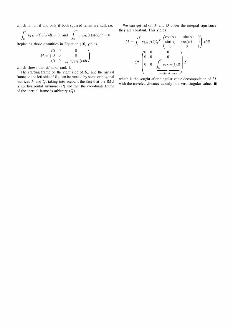
which is null if and only if both squared terms are null, i.e.∫ T

0

vIMU (t)c(α)dt = 0 and

∫ T

0

vIMU (t)s(α)dt = 0

Replacing those quantities in Equation (16) yields

M =

⎛⎝0 0 00 0 0

0 0∫ T

0vIMU (t)dt

⎞⎠

which shows that M is of rank 1.

The starting frame on the right side of Rα and the arrival

frame on the left side of Rα can be rotated by some orthogonal

matrices P and Q, taking into account the fact that the IMU

is not horizontal anymore (P ) and that the coordinate frame

of the inertial frame is arbitrary (Q).

We can get rid off P and Q under the integral sign since

they are constant. This yields

M =

∫ T

0

vIMU (t)QT

⎛⎝cos(α) − sin(α) 0sin(α) cos(α) 0

0 0 1

⎞⎠Pdt

= QT

⎛⎜⎜⎜⎜⎝0 0 00 0 0

0 0

∫ T

0

vIMU (t)dt︸ ︷︷ ︸traveled distance

⎞⎟⎟⎟⎟⎠P

which is the sought after singular value decomposition of Mwith the traveled distance as only non-zero singular value.