harvard economics math camp 2018: econometrics, probability … · harvard economics math camp...

Harvard Economics Math Camp 2018: Economet-rics, Probability ReviewAshesh Rambachan1

1 These notes are pull heavily frommaterials in many econometrics andstatistics textbooks (see referencesbelow) and draw heavily upon notesfrom other econometrics and statisticscourses (Max Kasy’s notes from Ec2110 at Harvard, Gary Chamberlain’snotes from Ec 2120, Mark Watson’snotes from ECON 517 at Princeton,Ramon van Handel’s notes from ORFE309 at Princeton and the University ofMinnesota’s math camp notes from Fall2015). I do not provide references in thetext. And so, I take ZERO credit and allerrors are my own.

August 2018

DISCLAIMERS:

1. There is absolutely no expectation for you to read these notes prior tomath camp. Maximize utility as you see fit.

2. This is intended to provide a brief refresher on some conceptsand preview some material that will be covered in the first yeareconometrics sequence. If some of the material is unfamiliar, do notworry.

3. These notes contain more content than we will have time to coverduring math camp. This is intentional. Hopefully these notes can bea useful reference material for you throughout the year.

Contents

Principles of Probability 3

Conditional Probability 4

Random Variables 7

Borel σ-algebra 7

Measurable functions 7

Random variables 7

Discrete random variables 8

Continuous random variables 9

Joint distributions 10

Transformations of Random Variables 11

Expectations 12

Conditional expectations 14

Moments and moment generating functions (MGFs) 15

Moments for random vectors 16

Useful Probability Distributions 17

Bernoulli distribution 17

Binomial distribution 17

Poisson distribution 17

Uniform distribution 18

harvard economics math camp 2018: econometrics, probability review 2

Univariate normal distribution 18

Chi-squared distribution 19

F-distribution 19

Student t-distribution 19

Exponential distribution 20

Multivariate Normal Distribution 20

Quadratic forms of normal random vectors 23

Jensen, Markov and Chebyshev, Oh My! 24


Principles of Probability

A random experiment is an experiment whose outcome cannotbe predicted beforehand. How do we model a random experiment?There are three key elements: The sample space, the events and theprobability measure. Each of these are described in turn.2 2 There are going to be a lot of defi-

nitions that seem overly complex todescribe something that seems fairlysimple... Bear with me and welcome toa Ph.D. in economics.

Definition 0.1. The sample space Ω is the set of all possible outcomes of arandom experiment. We denote an outcome as ω ∈ Ω.

Definition 0.2. An event A is a subset of the sample space, A ⊆ Ω. Let Adenote the family of all events.

Example 0.1. Suppose we survey 10 randomly selected people on theiremployment status and count how many are unemployed.

Ω = 0, 1, 2, . . . , 10

A is the event that more than 30% of those surveyed are unemployed.

A = 4, 5, 6, . . . , 10

Example 0.2. Suppose we ask a random person what is their income.

Ω = R+

A is the event that the person earns between $30, 000 and $40, 000.

A = [30, 000, 40, 000]

We place additional restrictions on A. These impose sufficientstructure that will allow us to consistently define the probabilities ofevents.

Definition 0.3. Let Ω be a set and A ⊆ 2Ω be a family of its subsets. F isa σ-algebra if and only if it satisfies the following

1. S ∈ F .

2. F is closed under complements: A ∈ F implies that AC = S− A ∈ F .

3. F is closed under countable union: If An ∈ F for n = 1, 2, . . ., then∪n An ∈ F .

Remark 0.1. Properties 1 and 2 of a σ-algebra implies that ∅ ∈ F . Proper-ties 2 and 3 imply that F is closed under countable intersection by DeMor-gan’s Law. That is, if An ∈ F for n = 1, 2, . . ., then ∩n An ∈ F .

We assume that A, the family of all events on Ω, is a σ-algebra. Wesay that (Ω,A) is measurable space and that A ∈ A is measurable withrespect to the σ-algebra A.


Definition 0.4. Let (Ω,A) be a measurable space. A measure is a func-tion, µ : A → R such that

1. µ(∅) = 0.

2. µ(A) ≥ 0 for all A ∈ A.

3. If An ∈ A for n = 1, 2, . . . with Ai ∩ Aj = ∅ for i 6= j, then

P(Un An) = ∑n

P(An)

If µ(Ω) < ∞, we call µ a finite measure, If µ(Ω) = 1, we call µ aprobability measure. We denote a probability measure as P : A → [0, 1].

Definition 0.5. A triple (Ω,A, µ) where Ω is a set, A is a σ-algebra andµ is a measure on A is a measure space. If µ is a probability measure, it isprobability space.

We’ve now defined all components needed to model a randomexperiments. A random experiment is characterized by its probabilityspace, (Ω,A, P). With the definition of a probability space that welaid out above, we can prove all of the usual probability facts.

Proposition 0.1. Consider a probability space (Ω,A, P). The followinghold:

1. For all A ∈ A, P(AC) = 1− P(A).

2. P(Ω) = 1.

3. If A1, A2 ∈ A with A1 ⊆ A2, then P(A1) ≤ P(A2).

4. For all A ∈ A, 0 ≤ P(A) ≤ P(1).

5. If A1, A2 ∈ A, then

P(A1 ∪ A2) = P(A1) + P(A2)− P(A1 ∩ A2)

Exercise 0.1. Prove these properties from the definition of a probabilityspace.

Conditional Probability

Conditional probability gives us a way to model the outcome of arandom experiment conditional on some partial information. Forinstance, given a random experiment and the information that eventB has occurred, what is the probability that the outcome also belongsto event A? To do so, we define a new probability measure on Ω.


Definition 0.6. Let A, B ∈ A with P(B) > 0. The conditional probabil-ity of A given B is

P(A|B) = P(A ∩ B)P(B)

P(A|B) is a probability measure.

Remark 0.2. We can think about P(A|B) as part of a new probability spacewith Ω = B and P(S) = P(S|B) for S ⊆ B.

Remark 0.3. Because the conditional probability is a probability measure,all of the usual properties of probability measures in Proposition 0.1 apply.

The definition of conditional probability implies the followinguseful formula. We have that

P(A ∩ B) = P(A|B)P(B) (1)

We next list several important results about conditional probabilities.

Theorem 0.1. The multiplication rule

P(∩ni=1 Ai) = P(A1)P(A2|A1)P(A3|A2 ∩ A1) . . . P(An| ∩n−1

i=1 Ai)

Proof. This follows via repeated application of the definition of con-ditional probability.

Theorem 0.2. Law of total probabilityConsider K disjoint events Ck that partition Ω. That is, Ci ∩ Cj = ∅ for

all i 6= j and ∪Ki=1Ci = Ω. Let C be some event.

P(C) =K

∑i=1

P(C|Ci)P(Ci)

Proof. We have that

C = C ∩Ω

= C ∩ (∪Ki=1Ci)

= (C ∩ C1) ∪ . . . ∪ (C ∩ CK)

It follows

P(C) =k

∑i=1

P(C ∩ Ci)

and the result follows from the definition of conditional probability.

Theorem 0.3. Bayes’ Rule

P(B|A) =P(A|B)P(B)

P(A|B)P(B) + P(A|BC)P(BC)


Exercise 0.2. Prove Bayes’ Rule from the results presented.

Example 0.3. Suppose you survey 2 randomly selected individuals. What isthe probability that both are female given that at least one is female? Assumethat all outcomes are equally likely.

Solution. The sample space is Ω = MM, MF, FM, FF. The condi-tioning event is B = MF, FM, FF and A = FF. Therefore,

P(A|B) = P(FF)P(MF, FM, FF) = 1/3

As mentioned, we use conditioning to describe the partial informa-tion that an event B gives about another event A. What if B providesno information about A?

Definition 0.7. Two events A, B are independent if

P(A|B) = P(A)

Equivalently, they are independent if

P(B|A) = P(B)

orP(A ∩ B) = P(A)P(B)

Remark 0.4. If events A, B are independent, then so are AC, B, A, BC andAC, BC.

We can extend the definition of independence to collections ofevents.

Definition 0.8. Let E1, . . . , En be events. E1, . . . , En are jointly indepen-dent if for any i1, . . . , ik

P(Ei1 |Ei2 ∩ . . . ∩ Eik ) = Ei1

Moreover, since conditional probabilities are probability measures,we can define independence with respect to a conditional probability.

Definition 0.9. Given an event C, events A, B are conditionally inde-pendent if

P(A ∩ B|C) = P(A|C)P(B|C)

Equivalently, A, B are independent conditional on C if

P(A|B ∩ C) = P(A|C)


Random Variables

Borel σ-algebra

Earlier in these notes, we defined a σ-algebra. This was a collectionof sets that satisfied some additional restrictions that helped us con-sistently define the probability of each set. A particularly importantσ-algebra is called the Borel σ-algebra. This is a σ-algebra over thereal line.

Definition 0.10. Let Ω = R. Let A be the collection of all open intervals.The smallest σ-algebra containing all open sets is the Borel σ-algebra. It istypically denoted as B.

Note that the Borel σ-algebra contains all closed intervals as welland could have been equivalently defined as the smallest σ-algebrathat contains all closed sets. Moreover, we can extend the Borel σ-algebra to higher dimensions - it is the smallest σ-algebra that con-tains the open balls. The Borel σ-algebra will be useful later on in thissection.

Measurable functions

A measurable function is a function that maps from one measurespace to another. Measurable functions are useful because for a givenset of values in the function’s range, we can measure the subset of thefunction’s domain upon which these values occur.

Definition 0.11. Let (Ω,A, µ) and (Ω′,A′, µ′) be two measure spaces. Letf : Ω → Ω′ be a function. f is measurable if and only if f−1(A′) ∈ A forall A′ ∈ A′.

That is, µ′( f−1(A′)) is well-defined for a measurable function f . Aparticularly useful case occurs when

(Ω′,A′, µ′) = (R,B, λ)

where λ is the lebesgue measure. That is, f is a real-valued function.We say that f is µ-measurable if and only if

f−1((−∞, c)) = ω ∈ Ω : f (ω) < c ∈ A ∀c ∈ R

We could also state this definition in terms of >,≤ or ≥. With thesedefinitions, we are now ready to define a random variable

Random variables

Consider a probability space (Ω,A, P). A random variable is simplya measurable function from the sample space Ω to the real-line.


Definition 0.12. Let (Ω,A, P) be a probability space and X : Ω → R is afunction. X is a random variable if and only if X is P-measurable. That is,X−1(B) ∈ A for all B ∈ B where B is the Borel σ-algebra.

Definition 0.13. Let X be a random variable. The cumulative distribu-tion function (cdf) F : R→ [0, 1] of X is defined as

FX(x) = P(X−1(x)) = P(ω ∈ Ω : X(ω) ≤ x)

For simplicity, we often write

FX(x) = P(X ≤ x)

Note that (R, B, FX) form a probability space. The cumulative distributionfunction FX has the following properties:

1. For x1 ≤ x2,

FX(x2)− FX(x1) = P(x1 < X < x2).

2. limx→−∞ FX(x) = 0, limx→∞ FX(x) = 1.

3. FX(x) is non-decreasing.

4. FX(x) is right-continuous: limx→x+0FX(x) = FX(x0).

Remark 0.5. Quantiles The quantiles of a random variable X are given bythe inverse of its cumulative distribution function. Generally, the quantilefunction is

Q(u) = infx : FX(x) ≥ u.

If FX is invertible, thenQ(u) = F−1

X (u).

Remark 0.6. For any function F that satisfies the properties of a cdf listedabove, we can construct a random variable whose cdf is F. Let U be uni-formly distributed on [0, 1]. That is, FU(u) = u for all u ∈ [0, 1]. DefineY = Q(U), where Q is the quantile function associated with F. In the case,where F is invertible, we have

FY(y) = P(F−1(U) ≤ y) = P(U ≤ F(y)) = F(y)

Discrete random variables

If FX is constant except at a countable number of points (i.e. FX is astep function), then we say that X is a discrete random variable. Thesize of the jump at xi

pi = FX(xi)− limx→x−i

FX(x)


is the probability that X takes on the value xi. That is,

P(X = xi) = pi

The probability mass function (pmf) of X is defined as

fX(x) =

pi if x = xi, i = 1, 2, . . .

0 otherwise

It follows that we can write

P(x1 < X ≤ x2) = ∑x1<x≤x2

fX(x).

Continuous random variables

If FX can be written as

FX(x) =∫ x

−∞fX(t)dt

where fX(x) satisfies

fX(x) ≥ 0 ∀x ∈ R∫ ∞

−∞fX(t)dt = 1,

we say that X is a continuous random variable. By the fundamentaltheorem of calculus, at the points where fX is continuous,

fX(x) =dFX(x)

dx.

We call fX(x) the probability density function (pdf) of X. We call

SX = x : fX(x) > 0

the support of X.Note that for x2 ≥ x1,

P(x1 < X ≤ x2) = FX(x2)− FX(x1)

=∫ x2

x1

fX(t)dt

and thatP(X = x) = 0

for a continuous random variable.

Remark 0.7. Do not interpret the pdf of a continuous random variable asexpressing a probability ( fX(x) 6= P(X = x)). The proper interpretationis that fX(x) expresses the probability that X falls in some small interval(x, x + ∆x). That is,

P(X ∈ (x, x + ∆x)) ≈ f (x)∆x


Joint distributions

Let X, Y be two scalar random variables. A random vector (X, Y) is amapping from Ω to R2.3 The joint cumulative distribution function 3 We can extend the formal definitions

for random variables to random vectors.(X, Y) is a random vector if and onlyif (X, Y) is P-measurable. That is,(X, Y)−1(B) ∈ A for all B ∈ B, where B

is now the Borel σ-algebra on R2.

of X, Y is

FX,Y(x, y) = P(X ≤ x, Y ≤ y)

= P(ω : X(ω) ≤ x ∩ ω : Y(ω) ≤ y)

We say that (X, Y) is a discrete random vector if

FX,Y(x, y) = ∑u≤x

∑v≤y

fX,Y(u, v),

where fX,Y(x, y) = P(X = x, Y = y) is the joint probability massfunction of (X, Y). We say that (X, Y) is a continuous random vectorif

FX,Y(x, y) =∫ x

−∞

∫ y

−∞fX,Y(u, v)dvdu,

where fX,Y(x, y) is the joint probability density function of (X, Y).As in the univariate case,

fX,Y(x, y) =∂2FX,Y(x, y)

∂x∂y

at the points of continuity of FX,Y. From the joint cdf of (X, Y), wecan recover the marginal cdfs. We have that

FX(x) = P(X ≤ x)

= P(X ≤ x, Y ≤ ∞)

= limy→∞

FX,Y(x, y).

We can also recover the marginal pdfs from the joint pdf using

fX(x) = ∑y

fX,Y(x, y) if discrete

, andfX(x) =

∫Sy

fX,Y(x, y)dy if continuous.

Consider the discrete case. Let x be such that fX(x) > 0. Then, theconditional pmf of Y given X = x is

fY|X(y|x) =fX,Y(x, y)

fX(x).

This satisfies the following two properties:

fY|X(y|x) ≥ 0

∑y

fY|X(y|x) = 1.


That is, fY|X(y|x) is a well-defined pmf for a discrete random vari-able. The conditional cdf of Y given X = x is then

FY|X(y|x) = P(Y ≤ y|X = x) = ∑v≤y

fY|X(v|x)

.Next, consider the continuous case. It is analogous. For any x such

that fX(x) > 0, the conditional pdf of Y given X = x is

fY|X(y|x) =fX,Y(x, y)

fX(x).

Provided that fX(x) > 0, this is a well-defined pdf for a continuousrandom variable. The conditional cdf is

FY|X(y|x) =∫ y

−∞fY|X(v|x)dv.

Remark 0.8. The conditional pmf for two discrete random variables can beinterpreted as a probability. That is, for the discrete random vector (X, Y),

fY|X(y|x) = P(Y = y|X = x).

However, this is not true for continuous random variables because if X iscontinuous, P(X = x) = 0. Instead, think about it as

fY|X(x, y) = P(X ∈ dx|Y = y)

= lim∆y→0

P(X ∈ dx|y ≤ Y ≤ y + dy)

Finally, we extend the definition of independence to random vari-ables. The random variables X, Y are independent if FY|X(y|x) =

FY(y) or equivalently, if FX,Y(x, y) = FX(x)FY(y). We can also definethis in terms of the densities. X, Y are independent if fY|X(y|x) =

fY(y) or equivalently, if fX,Y(x, y) = fX(x) fY(y).All of these definitions and results extend to n-dimensional ran-

dom variables in a straightforward manner.

Transformations of Random Variables

Let X be a random variable with cdf FX . Define the random variableY = h(X), where h is a one-to-one function whose inverse h−1 exists.What is the distribution of Y?

First, suppose that X is discrete and takes on values x1, . . . , xn. Y isalso discrete and takes on the values

yi = h(xi), for i = 1, . . . , n.

We have that the pmf of Y is given by

P(Y = yi) = P(X = h−1(xi))


fY(y) = fX(h−1(yi))

Next, suppose that X is continuous. Consider the case where h isincreasing. We have that

FY(y) = P(Y ≤ y)

= P(X ≤ h−1(y)) = FX(h−1(y)).

It follows directly that

fY(y) =dFY(y)

dy

= fX(h−1(y)dh−1(y)

dy

In the case were h is decreasing, we can analogously show that

fY(y) = − fX(h−1(y)dh−1(y)

dy

Combining these two cases, we have that, in general,

fY(y) = fx(h−1(y))|dh−1(y)dy

|

Example 0.4. Suppose X ∼ U[0, 1] and Y = X2. Over the support of X,this is a one-to-one transformation. We have that

X =√

Y, dX/dY =12

y−1/2.

Applying the formula above, we have that SY = [0, 1] and

fY(y) =12

y−1/2.

This can extended to the multivariate case. Let X be a randomvector and as before, define Y = h(X). You can show that

fY(y) = fX(h−1(x))|J|

where |J| is the absolute value of the determinant of the Jacobianmatrix of the inverse transformation. That is, |J| is the absolute valueof the determinant of the matrix whose i, j-th entry is ∂xi/∂yj.

Expectations

Suppose X is a discrete random variable. Its expectation or expectedvalue is defined as

E[X] = ∑x

x fX(x).


if ∑x |x| fX(x) < ∞. Otherwise, its expectation is said to not exist.Suppose X is a continuous random variable. Its expectation is de-fined as

E[X] =∫

SX

x fX(x)dx

if∫

SX|x| fX(x)dx < ∞. Otherwise, its expectation is said to not exist.4 4 Formally, the expectation is defined

using the Lebesgue-Stieltjes integral.We can also define the expectation of functions of random variables.Let g : R→ R. Then, if X is discrete,

E[g(X)] = ∑x

g(x) fX(x)

and if X is continuous, then

E[g(X)] =∫

SX

g(x) fX(x)dx.

The following are useful properties of the expectation operator.Suppose a, b ∈ R and g1(·), g2(·) are real-valued functions.

1. E[a] = a.

2. E[ag1(X)] = aE[g1(X)].

3. E[g1(X) + g2(X)] = E[g1(X)] + E[g2(X)].

These properties together imply that the expectation is a linear opera-tor.

We can use the expectation operator to express probabilities. Anindicator function 1(A) is a function that is equal to one if conditionA is true and zero otherwise. For example, if X is a random variable,then

1(X ≤ x) =

1 if X ≤ x

0 otherwise

Note that (for the continuous case)

E[1(X ≤ x)] =∫ ∞

−∞1(X ≤ x) fX(x)dx

=∫ x

−∞fX(x)dx

= FX(x) = P(X ≤ x).

More generally, if AX ⊆ R, we have that

E[1(X ∈ AX)] = P(X ∈ AX)

This is a very useful result.Suppose X, Y are random variables with joint density fX,Y(x, y).

Let g(x, y) : R2 → R. We have that

E[g(X, Y)] =∫ ∞

−∞g(x, y) fX,Y(x, y)dydx.


Note that by linearity of the expectation, for a, b ∈ R,

E[aX + bY] = aE[X] + bE[Y].

Finally, if X, Y are independent, then for any functions h1(·), h2(·),

E[h1(X)h2(Y)] = E[h1(X)]E[h2(Y)].

All of these results generalize directly to higher dimensions.

Conditional expectations

Given a pair of random variables (X, Y) with a joint density fX,Y(x, y),we can define the conditional expectation of Y given X = x as

E[Y|X = x] =∫

SY

y fY|X(y|x)dy.

Note that this is a function of x. It is sometimes denote µY(x) andcalled the regression function. In particular, this means we can viewthis a random function E[Y|X]. The following theorem is extremelyuseful. 5 5 This might be the most important

thing we cover in math camp!Theorem 0.4. The law of iterated expectations 6 6 This is also called the Tower Property.

EY[Y] = EXEY|X [Y],

where EX denotes the expectation taken with respect to the marginal densityof X and EY|X denotes the expectation taken with respect to the conditionaldensity of Y given X.

Proof. We have that

EXEY|X [Y] =∫ ( ∫

y fY|X(y)dy)

fX(x)dx

=∫ ∫

y fY|X(y) fX(x)dydx

=∫

y( ∫

fX,Y(x, y)dx)

dy

=∫

y fY(y)dy = E[Y]

What are some ways to interpret the conditional expectation? Weprovided a formal definition but we also want to provide some intu-ition. First, the conditional expectation is the solution to an optimalforecasting problem. Suppose you wish to forecast the value of a ran-dom variable Y. That is, we wish to pick h ∈ R that minimizes theexpected mean-square error

E[(Y− h)2] =∫(y− h)2 fY(y)dy.


The first-order condition is∫y fY(y)dy =

∫h fY(y)dy =⇒ h∗ = E[Y].

That is, the optimal prediction of Y is E[Y]. 7 Now, suppose that we 7 Optimal with respect to expectedmean-square error. If we changed theobjective function to expected mean-absolute error, E[|Y− h|], the solution isthe median of Y, h∗ = median(Y).

observe another random variable X and see that X = x. We wish toforecast Y as a function of x. That is, we wish to minimize

E[(Y− h(X))2].

Note that we can always write any function of X as

h(x) = µY(x) + g(x)

by defining g(x) = h(x)− µY(x). So choosing h to minimize expectedmean-square error is equivalent to choosing g. We can then write

(Y− h(X))2 = (Y− µY(X))2 − 2g(X)(Y− µY(x)) + g(X)2.

I claim that 8 8 Can you show these steps?

EY|X [g(X)(Y− µY(x))] = 0

and so,E[(Y− h(X))2] = E[(Y− µY(X))2 + g(X)2]

. It then follows immediately that expected mean-squared error isminimized with g(x) = 0 and so,

h∗(x) = µY(x).

That is, the conditional expectation of Y given X is the optimal pre-dictor of Y given X.9 9 And with that, you have learned a

good chunk of machine learning. I amnot joking.

Second, we can interpret the conditional expectation of Y givenX as the orthogonal projection of Y onto the space of functions ofthe random variable X i.e. L2 space. Since this interpretation of theconditional expectation is the focus of the first several lectures ofEcon 2120, I will not cover it here.

Moments and moment generating functions (MGFs)

Consider a random variable X. The k-th moment of X is defined asE[Xk]. The first moment of X is its mean, E[X]. The k-th centeredmoment of X is E[(X − E[X])k]. The second centered moment of X isits variance, V(X) = E[(X − E[X])2]. The standard deviation of X is√

V(X).

Remark 0.9. Suppose X has mean µX and variance σ2X . Let a, b ∈ R and

define Y = a + bX. Then,

µY = a + bµX , σ2Y = b2σ2

X .


Definition 0.14. The moment generating function (MGF) of a randomvariable X is defined as

µX(t) = E[etX ] =∫

etx fX(x)dx.

The MGF of X is useful because it allows us to easily compute allof the moments of a random variable. Note that

µ′X(t) =∫

xetx fX(x)dx, µ′X(0) =∫

x fX(x)dx = E[X],

µ′′X(t) =∫

x2etx fX(x)dx, µ′′X(0) =∫

x2 fX(x)dx = E[X2].

In general, we can show that

µ(j)X (0) = E[X j] for j = 1, 2, . . .

Moreover, the MGF of a random variable completely characterizesthe distribution of a random variable. If X, Y are two random vari-ables with the same MGF, then they have the same distribution.

Remark 0.10. The MGF may not always exist for a random variable.For example, etX may blow up for large realizations of X. However, thecharacteristic function of X is guaranteed to exist. It is defined as

E[eitx], i =√−1.

The characteristic function is guaranteed to exist and it completely charac-terizes the distributed of X.

Moments for random vectors

Suppose X, Y are two random variables with joint density fX,Y(x, y).The covariance between X, Y is defined as

Cov(X, Y) = E[(X− E[X])(Y− E[Y])]

= E[XY]− E[X]E[Y]

The covariance is a linear operator. That is,

Cov(X, aY + bW) = aCov(X, Y) + bCov(X, W).

Moreover, suppose Z = aX + bY for a, b ∈ R. Then,

V(Z) = a2V(X) + b2V(Y) + 2abCov(X, Y).

Now suppose that X is an n-dimensional random vector withX = (X1, . . . , Xn). Its mean vector is

E[X] =

E[X1]

...E[Xn]


and its covariance matrix is

V(X) = Σ

where Σ is an n × n matrix whose ij-th entry is Σij = Cov(Xi, Xj).Σ is a positive semi-definite matrix. Why? Let α ∈ Rn and defineY = αTX. Then,

V(Y) = αTΣα ≥ 0.

This must hold for all α ∈ Rn.

Useful Probability Distributions

Bernoulli distribution

X is a discrete random variable that can only take on two values: 0, 1.We write fX(1) = p, fX(0) = 1− p and so,

fX(x) = px(1− p)1−x.

Note that

E[Xk] = p, k ≥ 1

V(X) = p(1− p),

µX(t) = (1− p) + pet.

We say that X has a Bernoulli distribution.

Binomial distribution

Suppose that Xi for i = 1, . . . , n are i.i.d Bernoulli random variableswith P(Xi = 1) = p. Define X = ∑n

i=1 Xi. We say that X follows abinomial distribution with parameters n and p. X takes on values1, 2, . . . , n. Its pmf is

fX(x) =(

nx

)px(1− p)n−x

andE[X] = np, V(X) = np(1− p).

Poisson distribution

Suppose that X is a discrete random variables and takes on values1, 2, 3, . . .. Its pmf is

fX(x) =λxe−λ

x!, λ > 0


We say that X is a Poisson random variable with parameter λ > 0.Note that

E[X] = λ, V(X) = λ.

Poisson random variables are typically used to model the number ofdiscrete "successes" that occur over a time period.

Remark 0.11. Note that if Xn is binomially distributed with parameters

n, p = λ/n, then Xnd−→ X, where X is a Poisson random variable.10 10 The notation Xn

d−→ X means thatthe sequence of random variables Xn"converges in distribution" to the ran-dom variable X. We have not formallydefined this yet but intuitively, it meansthat as n gets large, Xn behaves as if itwere distributed like X.

Uniform distribution

Suppose that X is a continuous random variable with fX(x) = 1b−a

for x ∈ [a, b] and 0 otherwise. We say that X is uniformly distributedon [a, b] and write X ∼ U[a, b].

Univariate normal distribution

Suppose Z is continuously distributed with support over R. We saythat X follows a standard normal distribution if

fZ(z) =1√2π

e−12 z2

We write Z ∼ N(0, 1) where E[Z] = 0, V(Z) = 1. We say that X ∼N(µ, σ2) if fX(x) = 1√

2πσ2 e−1

2σ2 (x−µ)2Note that E[X] = µ, V(X) = σ2

and X = µ + σZ, where Z ∼ N(0, 1).The MGF of a standard normal random variable is incredibly

useful. 11 It is worth memorizing. If Z ∼ N(0, 1), then 11 For example, you’ll run into it all thetime in macro/finance.

MZ(t) = e12 t2

.

Why? Here’s the calculation: 12 12 It’s straightforward provided youremember how to complete the square.

MZ(t) = E[etZ]

=∫ ∞

−∞etz 1√

2πe−

12 z2

dz

=∫ ∞

−∞

1√2π

etz− 12 z2

dz

=∫ ∞

−∞

1√2π− 1

2e−

12 (z

2−2tz)dz

= e12 t2∫ ∞

−∞

1√2π

e−12 (z

2−2tz+t2)dz

= e12 t2∫ ∞

−∞

1√2π

e−12 (z−t)2

dz

= e12 t2∫ ∞

−∞

1√2π

e−12 (w)2

dz, w = z− t

= e12 t2


We can use this to derive the MGF for X ∼ N(µ, σ2). We have that

MX(t) = E[etX ]

= E[et(µ+σZ)]

= etµE[etσZ]

= etµ MZ(tσ)

= eµt+ 12 σ2t2

Therefore, we have that

MX(t) = eµt+ 12 σ2t2

.

Chi-squared distribution

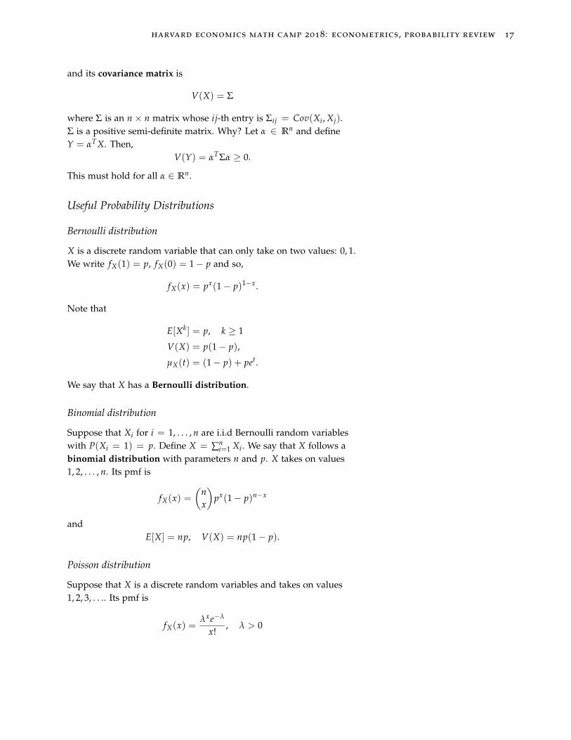
Let Zi ∼ N(0, 1) i.i.d. for i = 1, . . . , n. Let

X =n

∑i=1

Z2i .

We say that X is a chi-squared random variable with n degrees offreedom and write X ∼ χ2

n. It follows immediately that

E[X] = n, V(X) = 2n

.

Figure 1: Density of χ2 as degree offreedom varies. (Source: Wikipedia)

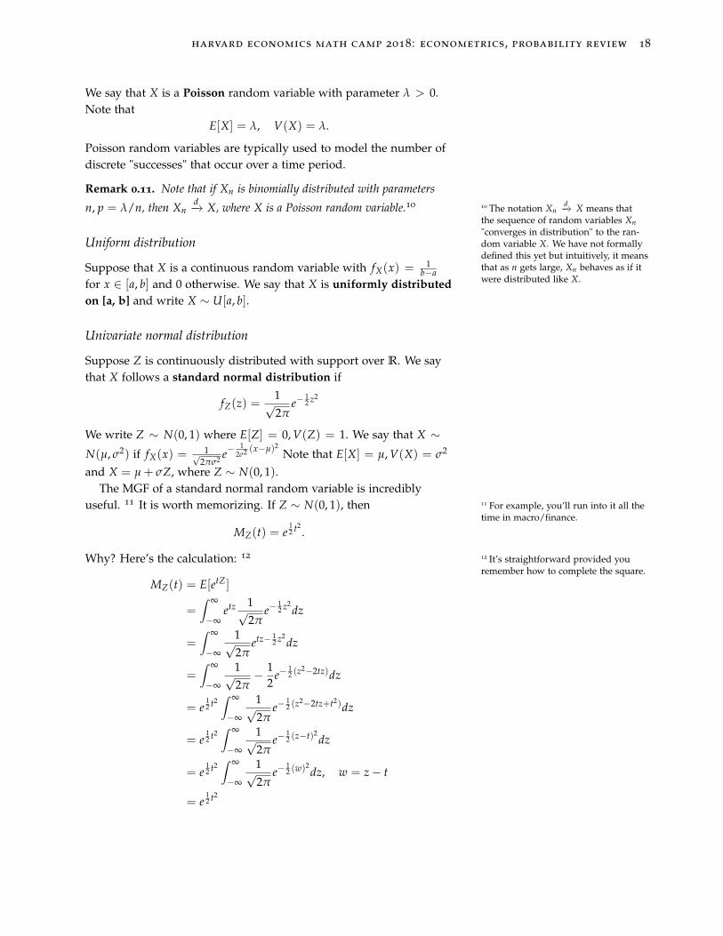
F-distribution

Let Y1 ∼ χ2k , Y2 ∼ χ2

l with Y1 ⊥ Y2. Define

Q =Y1/kY2/l

.

We say that Q follows an F-distribution with k, l degrees of freedom.We write Q ∼ Fk,l .

Figure 2: Density of Fk,l as degrees offreedom vary. (Source: Wikipedia)

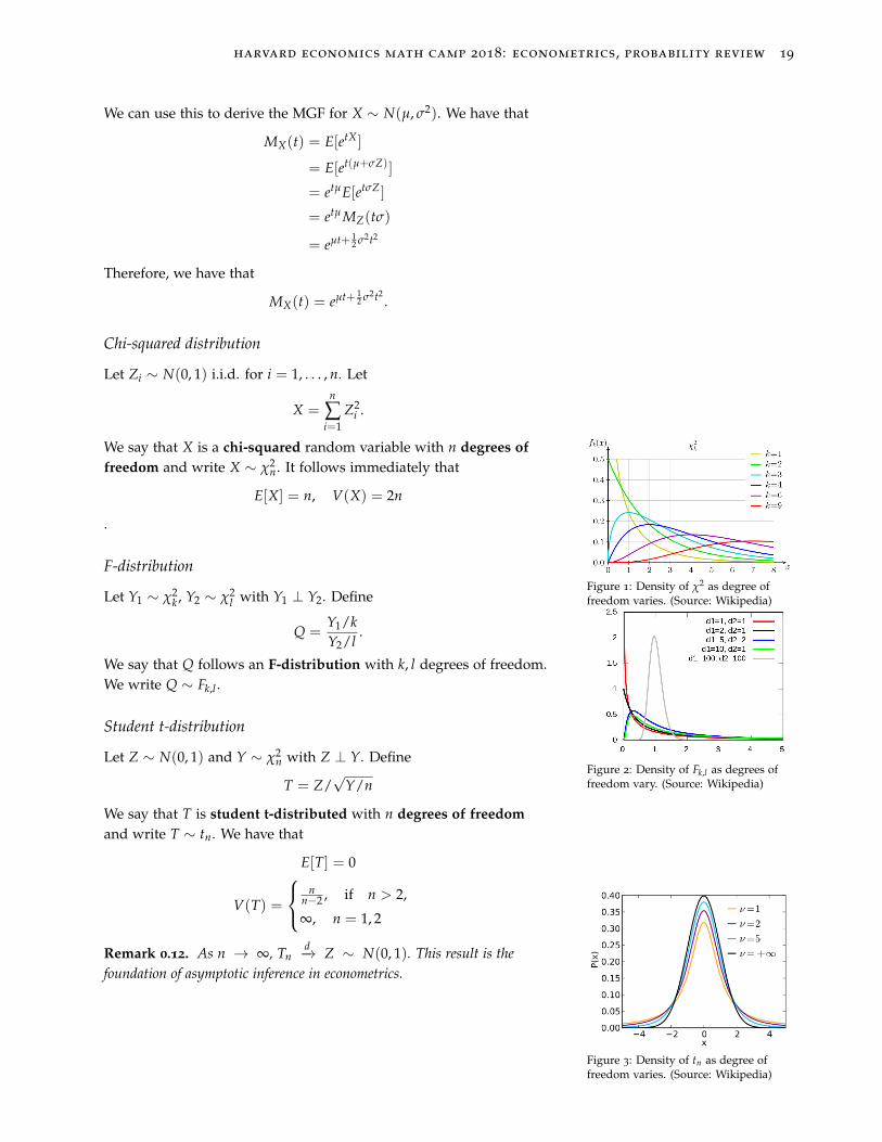
Student t-distribution

Let Z ∼ N(0, 1) and Y ∼ χ2n with Z ⊥ Y. Define

T = Z/√

Y/n

We say that T is student t-distributed with n degrees of freedomand write T ∼ tn. We have that

E[T] = 0

V(T) =

nn−2 , if n > 2,

∞, n = 1, 2

Remark 0.12. As n → ∞, Tnd−→ Z ∼ N(0, 1). This result is the

foundation of asymptotic inference in econometrics.

Figure 3: Density of tn as degree offreedom varies. (Source: Wikipedia)


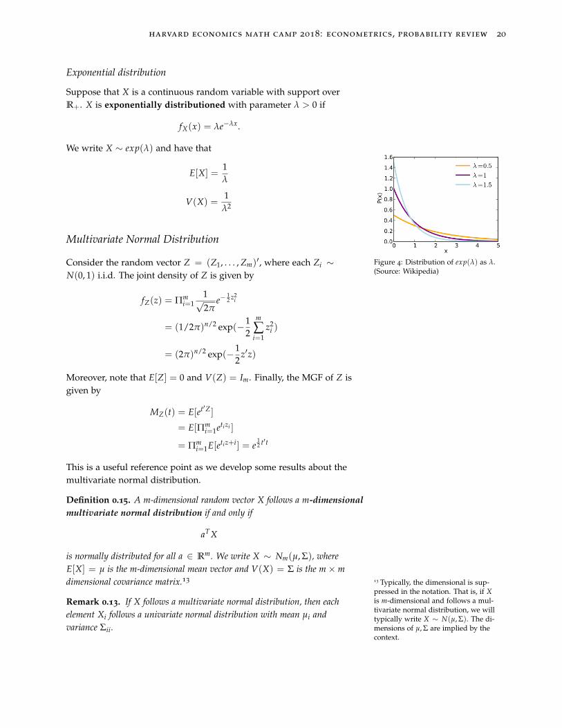
Exponential distribution

Suppose that X is a continuous random variable with support overR+. X is exponentially distributioned with parameter λ > 0 if

fX(x) = λe−λx.

We write X ∼ exp(λ) and have that

E[X] =1λ

V(X) =1

λ2

Figure 4: Distribution of exp(λ) as λ.(Source: Wikipedia)

Multivariate Normal Distribution

Consider the random vector Z = (Z1, . . . , Zm)′, where each Zi ∼N(0, 1) i.i.d. The joint density of Z is given by

fZ(z) = Πmi=1

1√2π

e−12 z2

i

= (1/2π)n/2 exp(−12

m

∑i=1

z2i )

= (2π)n/2 exp(−12

z′z)

Moreover, note that E[Z] = 0 and V(Z) = Im. Finally, the MGF of Z isgiven by

MZ(t) = E[et′Z]

= E[Πmi=1etizi ]

= Πmi=1E[etiz+i] = e

12 t′t

This is a useful reference point as we develop some results about themultivariate normal distribution.

Definition 0.15. A m-dimensional random vector X follows a m-dimensionalmultivariate normal distribution if and only if

aTX

is normally distributed for all a ∈ Rm. We write X ∼ Nm(µ, Σ), whereE[X] = µ is the m-dimensional mean vector and V(X) = Σ is the m× mdimensional covariance matrix.13 13 Typically, the dimensional is sup-

pressed in the notation. That is, if Xis m-dimensional and follows a mul-tivariate normal distribution, we willtypically write X ∼ N(µ, Σ). The di-mensions of µ, Σ are implied by thecontext.

Remark 0.13. If X follows a multivariate normal distribution, then eachelement Xi follows a univariate normal distribution with mean µi andvariance Σii.


Remark 0.14. It is important to have a good handle on the properties of theunivariate and multivariate normal distributions. When we use asymptoticsto approximate the finite-sample distribution of estimators and test-statisticsin econometrics, everything "becomes" normally distributed by the centraltheorem. 14 14 Not literally everything but you get

the point.The next two results will allow us to derive the distribution of a

multivariate normal. We first derive its MGF.

Proposition 0.2. Suppose X ∼ N(µ, Σ). Then,

MX(t) = et′µ+ 12 t′Σt.

Proof. Note that t′X ∼ N(t′µ, t′Σt). Therefore,

MX(t) = E[et′X ]

= E[eY], Y ∼ N(t′µ, t′Σt)

= MY(1)

and the result follows.

Recall that for a univariate normal distribution, if X ∼ N(µ, σ2), thenY = aX + b ∼ N(aµ + b, a2σ2). The same property holds for themultivariate normal distribution.

Proposition 0.3. Suppose X ∼ Nm(µ, Σ). Define

Y = AX + b,

where A ∈ Rn×m, b ∈ Rn. Then,

Y ∼ Nn(Aµ + b, AΣA′).

Proof. For t ∈ Rn,

MY(t) = E[et′Y]

= E[et′(AX+b)]

= et′bE[e(A′t)′X

= et′be(A′t)′µ+ 12 (A′t)′Σ(A′t)′

= et′(Aµ+b)+ 12 t′(AΣA′)t

We’ll now use the two previous results to derive the density of amultivariate normal distribution.

Proposition 0.4. Suppose X ∼ N(µ, Σ) and Σ has full column rank. Then,the density of X is given by

fX(x) = (2π)−m/2|Σ|−1/2 exp(−12(x− µ)′Σ−1(x− µ)).


Proof. Let Z be a m-dimensional random vector of i.i.d. standard nor-mal random variables. At the beginning of this section, we derivedthat MZ(t) = e

12 t′t. Therefore, Z ∼ Nm(0, Im). We also derived that

the density of Z isfZ(z) = (2π)−m/2e−

12 z′z.

Let X = µ + Σ1/2Z. We can show that X ∼ Nm(µ, Σ). From themultivariate transformation of random variables formula from anearlier section,

fX(x) = |Σ|−1/2 fZ(Σ−1/2(x− µ))

and the result follows.

The rest of this section lists additional useful properties of themultivariate normal distribution that will appear from time to time.It’s useful to be familiar with them.

Proposition 0.5. If X1 ∼ Nm(µ1, Σ1), X2 ∼ Nn(µ2, Σ2) and X1 ⊥ X2,then

X = (X′1, X′2)′ ∼ Nm+n(µ, Σ)

where

µ =

(µ1

µ2

), Σ =

(Σ1 00 Σ2

)

Proposition 0.6. Let X ∼ Nm(µ, Σ). Let X1 be a p-dimensional sub-vectorof X with p < m. Write

X =

(X1

X2

)and

µ =

(µ1

µ2

), Σ =

(Σ11 Σ12

Σ21 Σ22

).

Then, X1 ∼ Np(µ1, Σ11).

Proposition 0.7. Let X ∼ Nm(µ, Σ). Partition X into two sub-vectors.That is, write

X =

(X1

X2

)and

µ =

(µ1

µ2

), Σ =

(Σ11 Σ12

Σ21 Σ22

).

Then, X1 ⊥ X2 if and only if Σ12 = Σ21 = 0.


Proposition 0.8. Let X ∼ Nm(µ, Σ). If

Y = AX + b, V = CX + d,

where A, C ∈ Rn×m and b, d ∈ Rn, then

Cov(Y, V) = AΣC′.

Moreover, Y ⊥ V if and only if

AΣC′ = 0.

Exercise 0.3. Prove these properties of the multivariate normal distribution.

Proposition 0.9. Let X ∼ Nm(µ, Σ) with X = (X′1, X′2)′, µ = (µ′1, µ′2)

′

and

Σ =

(Σ11 Σ12

Σ21 Σ22

).

Provided that Σ22 has full rank, the conditional distribution of X1 givenX2 = x2 is

X1|X2 = x2 ∼ N(µ1 + Σ12Σ−122 (x2 − µ2), Σ11 − Σ12Σ−1

22 Σ21).

Remark 0.15. What’s the intuition of this? We have that

E[X1|X2 = x2] = µ1 + Σ12Σ−122 (x2 − µ2).

This formula will look more familiar if everything is one-dimensional. Itbecomes

E[X1|X2 = x2] = E[X1] +Cov(X1, X2)

V(X2)(x2 − E[X2])

Is this starting to look more familiar? Not yet? Ok, let’s relabel Y =

X1, X = X2 and re-arrange. Then,

E[Y|X = x] = (E[Y]− Cov(Y, X)

V(X)E[X]) +

Cov(Y, X)

V(X)x.

This is simply the linear regression formula!15 For a multivariate normal 15 Set β0 = E[Y] − Cov(Y,X)V(X)

E[X] and

β1 = Cov(Y,X)V(X)

. Then, E[Y|X = x] =β0 + β1x.

random distribution, conditional expectations are exactly linear. As a result,linear regression exactly returns the conditional expectation function.

This final result provides the conditional distribution of a multivari-ate normal distribution. This appears at random points throughoutthe first year and so, it is useful to keep in your back pocket.

Quadratic forms of normal random vectors

Recall that a quadratic form is a quantity of the form y′Ay, whereA is a symmetric matrix. Suppose that Zi ∼ N(0, 1) i.i.d. for i =

1, . . . , n. We already know that ∑ni=1 Z2

i = Z′Z ∼ χ2n.

Proposition 0.10. If X ∼ Nm(µ, Σ) and Σ has full rank, then

(X− µ)′Σ−1(X− µ) ∼ χ2m.

Proof. Let Z = Σ−1/2(X− µ) ∼ Nm(0, Im). Then, Z′Z ∼ χ2m.


Jensen, Markov and Chebyshev, Oh My!

The following are some useful inequalities that pop up in a varietyof contexts in econometrics and other areas of economics. These areespecially useful in asymptotics.

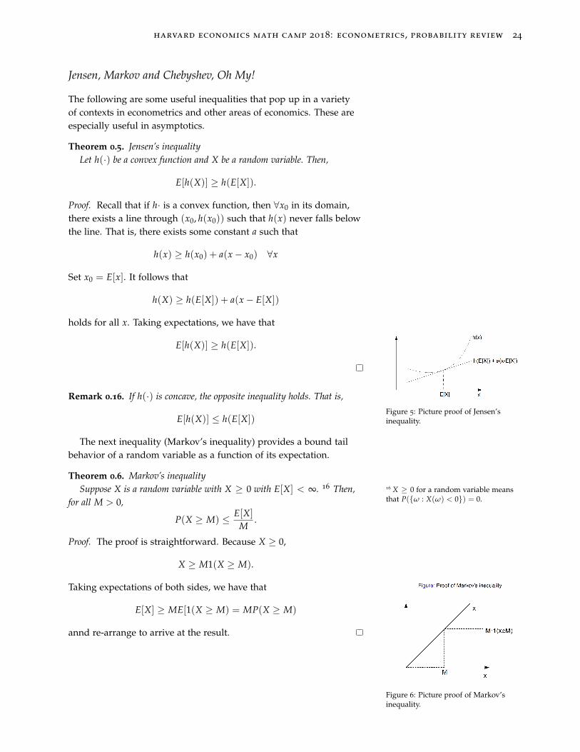
Theorem 0.5. Jensen’s inequalityLet h(·) be a convex function and X be a random variable. Then,

E[h(X)] ≥ h(E[X]).

Proof. Recall that if h· is a convex function, then ∀x0 in its domain,there exists a line through (x0, h(x0)) such that h(x) never falls belowthe line. That is, there exists some constant a such that

h(x) ≥ h(x0) + a(x− x0) ∀x

Set x0 = E[x]. It follows that

h(X) ≥ h(E[X]) + a(x− E[X])

holds for all x. Taking expectations, we have that

E[h(X)] ≥ h(E[X]).

Figure 5: Picture proof of Jensen’sinequality.

Remark 0.16. If h(·) is concave, the opposite inequality holds. That is,

E[h(X)] ≤ h(E[X])

The next inequality (Markov’s inequality) provides a bound tailbehavior of a random variable as a function of its expectation.

Theorem 0.6. Markov’s inequalitySuppose X is a random variable with X ≥ 0 with E[X] < ∞. 16 Then, 16 X ≥ 0 for a random variable means

that P(ω : X(ω) < 0) = 0.for all M > 0,

P(X ≥ M) ≤ E[X]

M.

Proof. The proof is straightforward. Because X ≥ 0,

X ≥ M1(X ≥ M).

Taking expectations of both sides, we have that

E[X] ≥ ME[1(X ≥ M) = MP(X ≥ M)

annd re-arrange to arrive at the result.

Figure 6: Picture proof of Markov’sinequality.


Example 0.5. Suppose that household income is non-negative. By Markov’sinequality, no more than 1/5 of households can have an income that isgreater than five times the average household income.

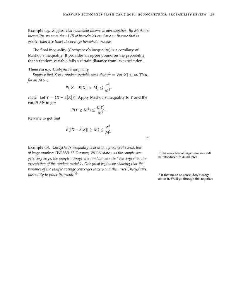
The final inequality (Chebyshev’s inequality) is a corollary ofMarkov’s inequality. It provides an upper bound on the probabilitythat a random variable falls a certain distance from its expectation.

Theorem 0.7. Chebyshev’s inequalitySuppose that X is a random variable such that σ2 = Var[X] < ∞. Then,

for all M > 0,

P(|X− E[X]| > M) ≤ σ2

M2 .

Proof. Let Y = (X − E[X])2. Apply Markov’s inequality to Y and thecutoff M2 to get

P(Y ≥ M2) ≤ E[Y]M2 .

Rewrite to get that

P(|X− E[X]| ≥ M) ≤ σ2

M2

Example 0.6. Chebyshev’s inequality is used in a proof of the weak lawof large numbers (WLLN). 17 For now, WLLN states: as the sample size 17 The weak law of large numbers will

be introduced in detail later.gets very large, the sample average of a random variable "converges" to theexpectation of the random variable. One proof begins by showing that thevariance of the sample average converges to zero and then uses Chebyshev’sinequality to prove the result.18 18 If that made no sense, don’t worry

about it. We’ll go through this together.


References

Billingsley, P. (2012). Probability and Measure.Blitzstein, J. and J. Hwang. (2014). Introduction to Probability.Casella, G. and R. Berger. (2001). Statistical Inference.Hogg, R., McKean, J. and A. Craig. (2012). Introduction to Mathemati-cal Statistics.Kolmogorov, A. and Fomin, S. (2012). Introductory Real Analysis.Stokey, N., Lucas, R. and E. Prescott. (1989). Recursive Methods inEconomic Dynamics.

harvard economics math camp 2018: econometrics, probability … · harvard economics math camp...

Documents