hashing cse 373 data structures lecture 10. 4/18/03hashing - lecture 102 readings reading ›chapter...

Hashing

CSE 373

Data Structures

Lecture 10

4/18/03 Hashing - Lecture 10 2

Readings

• Reading › Chapter 5


The Need for Speed

• Data structures we have looked at so far› Use comparison operations to find items› Need O(log N) time for Find and Insert

• In real world applications, N is typically between 100 and 100,000 (or more)› log N is between 6.6 and 16.6

• Hash tables are an abstract data type designed for O(1) Find and Inserts


Fewer Functions Faster

• compare lists and stacks› by reducing the flexibility of what we are allowed to do,

we can increase the performance of the remaining operations

› insert(L,X) into a list versus push(S,X) onto a stack

• compare trees and hash tables› trees provide for known ordering of all elements› hash tables just let you (quickly) find an element


Limited Set of Hash Operations

• For many applications, a limited set of operations is all that is needed› Insert, Find, and Delete› Note that no ordering of elements is implied

• For example, a compiler needs to maintain information about the symbols in a program› user defined› language keywords


Direct Address Tables

• Direct addressing using an array is very fast• Assume

› keys are integers in the set U={0,1,…m-1}› m is small› no two elements have the same key

• Then just store each element at the array location array[key]› search, insert, and delete are trivial


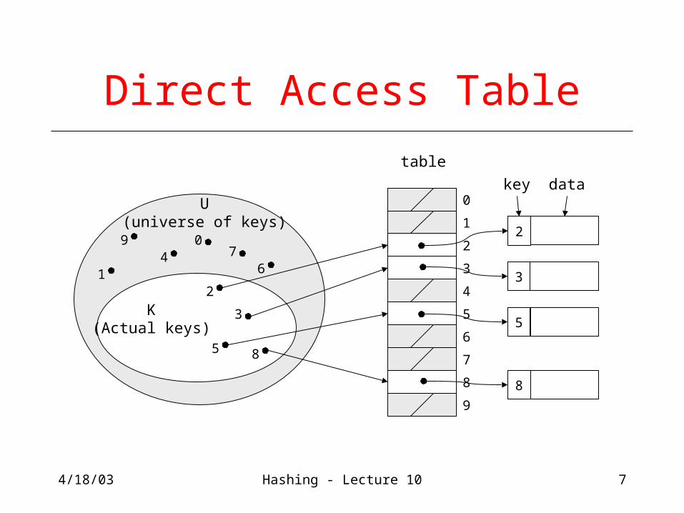
Direct Access Table

U(universe of keys)

K(Actual keys)

2

5 8

3

1

94

07

6

0

1

2

3

4

5

6

7

8

9

2

5

8

3

datakey

table


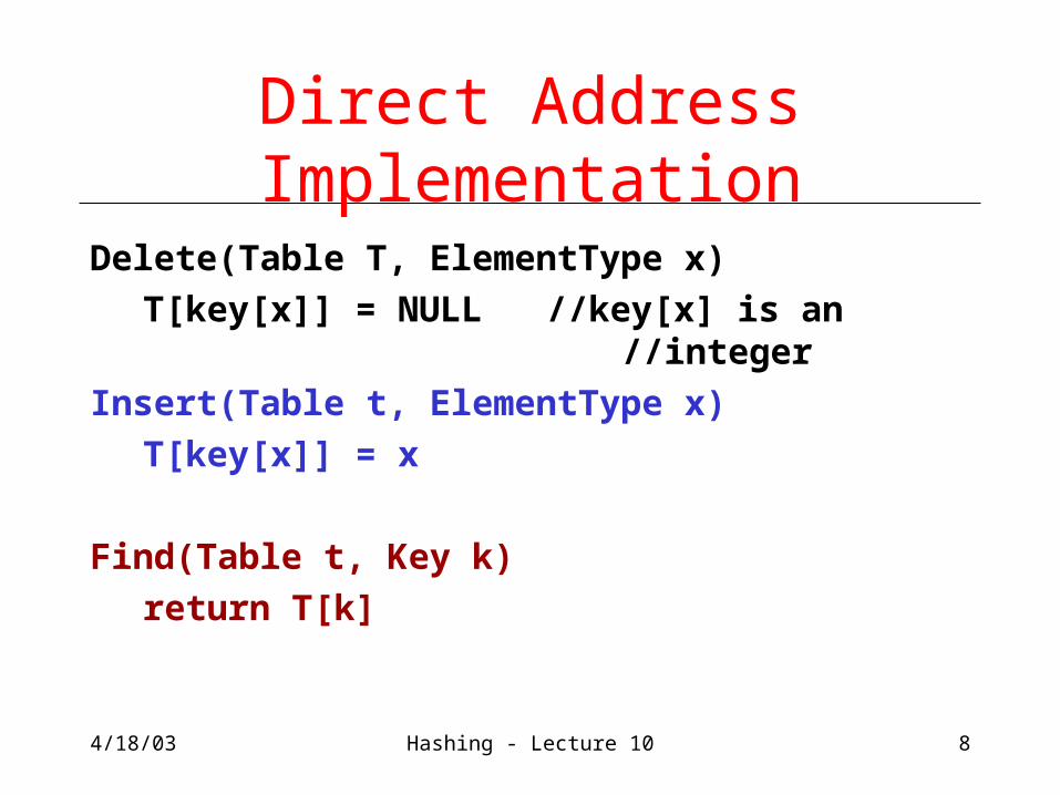
Direct Address Implementation

Delete(Table T, ElementType x)

T[key[x]] = NULL //key[x] is an //integer

Insert(Table t, ElementType x)

T[key[x]] = x

Find(Table t, Key k)

return T[k]


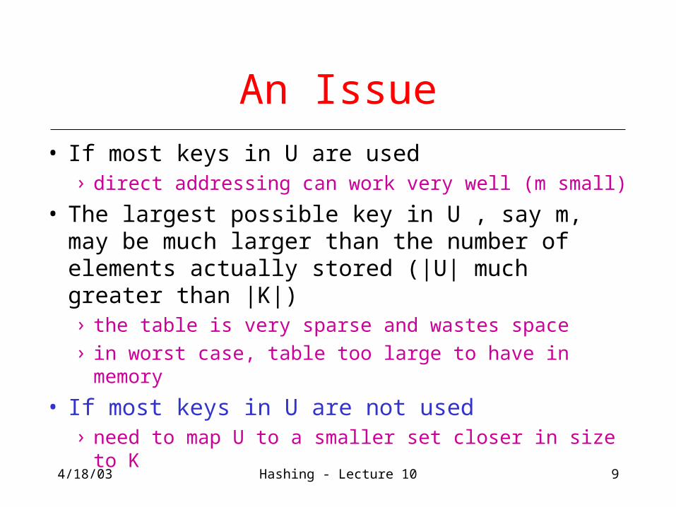
An Issue

• If most keys in U are used› direct addressing can work very well (m small)

• The largest possible key in U , say m, may be much larger than the number of elements actually stored (|U| much greater than |K|)› the table is very sparse and wastes space› in worst case, table too large to have in memory

• If most keys in U are not used› need to map U to a smaller set closer in size to K


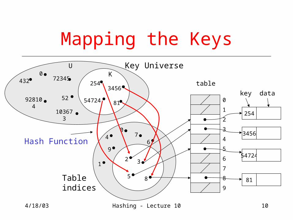
Mapping the KeysU

2

5 8

31

9

40

76

0

1

2

3

4

5

6

7

8

9

254

datakey

table254

54724 81

3456

103673

928104

4320

72345

52

K

Hash Function3456

54724

81

Key Universe

Tableindices


Hashing Schemes

• We want to store N items in a table of size M, at a location computed from the key K (which may not be numeric!)

• Hash function› Method for computing table index from key

• Need of a collision resolution strategy› How to handle two keys that hash to the

same index


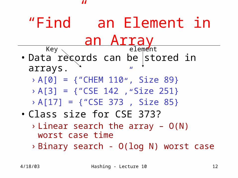
“Find” an Element in an Array

• Data records can be stored in arrays.› A[0] = {“CHEM 110”, Size 89}› A[3] = {“CSE 142”, Size 251} › A[17] = {“CSE 373”, Size 85}

• Class size for CSE 373?› Linear search the array – O(N) worst case

time› Binary search - O(log N) worst case

Key element


Go Directly to the Element

• What if we could directly index into the array using the key?› A[“CSE 373”] = {Size 85}

• Main idea behind hash tables› Use a key based on some aspect of the

data to index directly into an array› O(1) time to access records


Indexing into Hash Table

• Need a fast hash function to convert the element key (string or number) to an integer (the hash value) (i.e, map from U to index)› Then use this value to index into an array› Hash(“CSE 373”) = 157, Hash(“CSE 143”) = 101

• Output of the hash function› must always be less than size of array› should be as evenly distributed as possible


Choosing the Hash Function

• What properties do we want from a hash function?› Want universe of hash values to be

distributed randomly to minimize collisions› Don’t want systematic nonrandom pattern

in selection of keys to lead to systematic collisions

› Want hash value to depend on all values in entire key and their positions


The Key Values are Important

• Notice that one issue with all the hash functions is that the actual content of the key set matters

• The elements in K (the keys that are used) are quite possibly a restricted subset of U, not just a random collection› variable names, words in the English

language, reserved keywords, telephone numbers, etc, etc


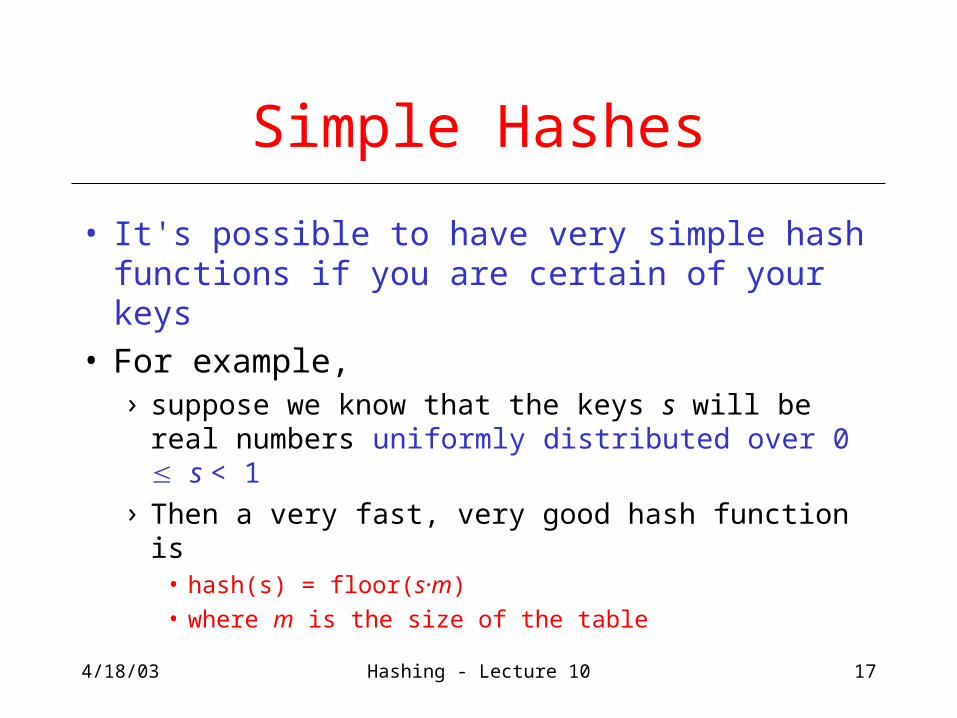
Simple Hashes

• It's possible to have very simple hash functions if you are certain of your keys

• For example, › suppose we know that the keys s will be real

numbers uniformly distributed over 0 s < 1› Then a very fast, very good hash function is

• hash(s) = floor(s·m)• where m is the size of the table


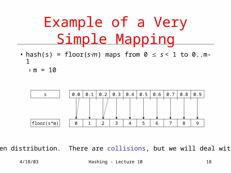
Example of a Very Simple Mapping

• hash(s) = floor(s·m) maps from 0 s < 1 to 0..m-1› m = 10

0.0 0.1 0.2 0.3 0.4 0.5 0.6 0.7 0.8 0.9

0 1 2 3 4 5 6 7 8 9

s

floor(s*m)

Note the even distribution. There are collisions, but we will deal with them later.


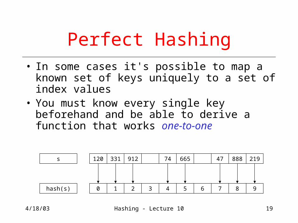
Perfect Hashing• In some cases it's possible to map a known set

of keys uniquely to a set of index values• You must know every single key beforehand

and be able to derive a function that works one-to-one

120 331 912 74 665 47 888 219

0 1 2 3 4 5 6 7 8 9

s

hash(s)


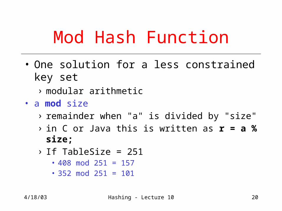
Mod Hash Function

• One solution for a less constrained key set› modular arithmetic

• a mod size› remainder when "a" is divided by "size"› in C or Java this is written as r = a % size;› If TableSize = 251

• 408 mod 251 = 157• 352 mod 251 = 101


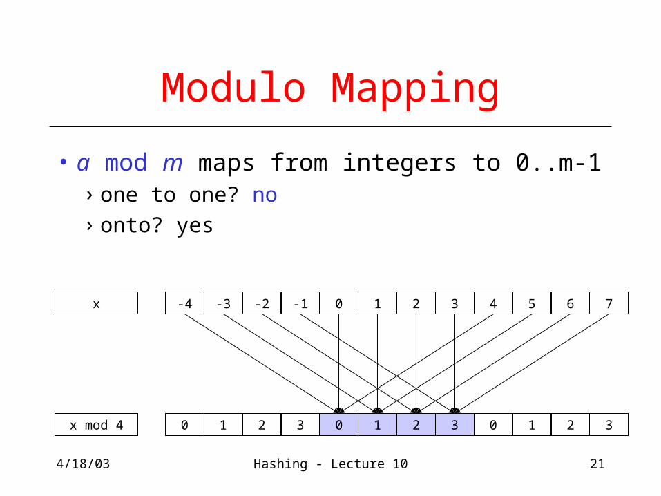
Modulo Mapping

• a mod m maps from integers to 0..m-1› one to one? no› onto? yes

-4 -3 -2 -1 0 1 2 3 4 5 6 7

0 1 2 3 0 1 2 3 0 1 2 3

x

x mod 4


Hashing Integers

• If keys are integers, we can use the hash function:› Hash(key) = key mod TableSize

• Problem 1: What if TableSize is 11 and all keys are 2 repeated digits? (eg, 22, 33, …)› all keys map to the same index› Need to pick TableSize carefully: often, a prime

number


Nonnumerical Keys

• Many hash functions assume that the universe of keys is the natural numbers N={0,1,…}

• Need to find a function to convert the actual key to a natural number quickly and effectively before or during the hash calculation

• Generally work with the ASCII character codes when converting strings to numbers


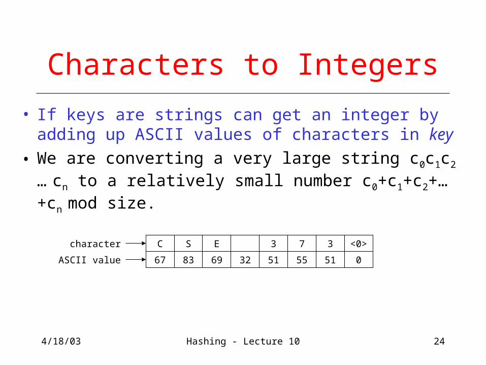
• If keys are strings can get an integer by adding up ASCII values of characters in key

• We are converting a very large string c0c1c2 … cn to a relatively small number c0+c1+c2+…+cn mod size.

Characters to Integers

67 83 69 32 51 55

C S E 3 7

ASCII value

character

51 0

3 <0>


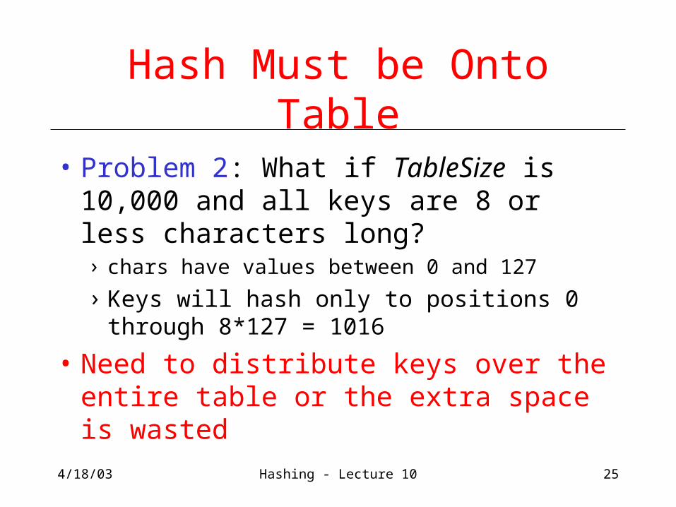
Hash Must be Onto Table

• Problem 2: What if TableSize is 10,000 and all keys are 8 or less characters long?› chars have values between 0 and 127

› Keys will hash only to positions 0 through 8*127 = 1016

• Need to distribute keys over the entire table or the extra space is wasted


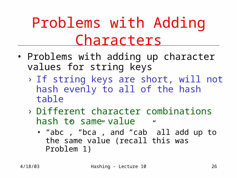
Problems with Adding Characters

• Problems with adding up character values for string keys› If string keys are short, will not hash

evenly to all of the hash table› Different character combinations hash to

same value• “abc”, “bca”, and “cab” all add up to the same

value (recall this was Problem 1)


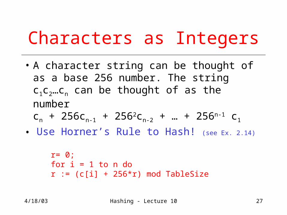
Characters as Integers

• A character string can be thought of as a base 256 number. The string c1c2…cn can be thought of as the number cn + 256cn-1 + 2562cn-2 + … + 256n-1 c1

• Use Horner’s Rule to Hash! (see Ex. 2.14)

r= 0;for i = 1 to n dor := (c[i] + 256*r) mod TableSize


Collisions

• A collision occurs when two different keys hash to the same value› E.g. For TableSize = 17, the keys 18 and

35 hash to the same value for the mod17 hash function

› 18 mod 17 = 1 and 35 mod 17 = 1

• Cannot store both data records in the same slot in array!


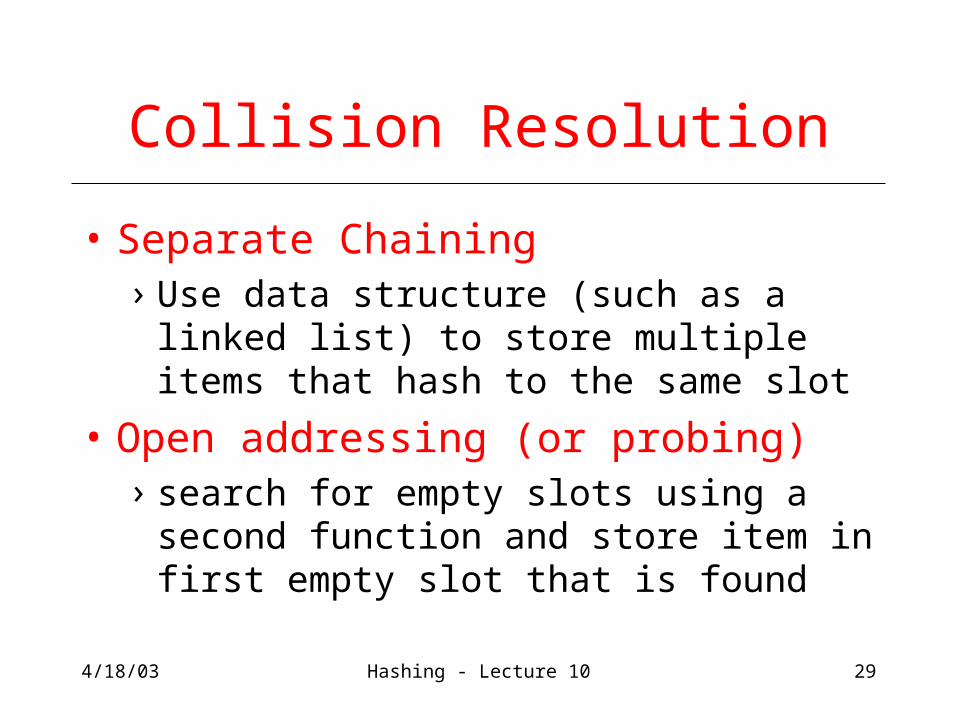
Collision Resolution

• Separate Chaining› Use data structure (such as a linked list) to

store multiple items that hash to the same slot

• Open addressing (or probing)› search for empty slots using a second

function and store item in first empty slot that is found


Resolution by Chaining

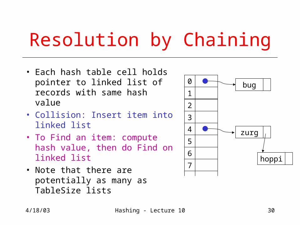
• Each hash table cell holds pointer to linked list of records with same hash value

• Collision: Insert item into linked list

• To Find an item: compute hash value, then do Find on linked list

• Note that there are potentially as many as TableSize lists

0

1

2

3

4

5

6

7

bug

zurg

hoppi


Why Lists?

• Can use List ADT for Find/Insert/Delete in linked list› O(N) runtime where N is the number of elements

in the particular chain

• Can also use Binary Search Trees› O(log N) time instead of O(N)› But the number of elements to search through

should be small (otherwise the hashing function is bad or the table is too small)

› generally not worth the overhead of BSTs


Load Factor of a Hash Table

• Let N = number of items to be stored• Load factor = N/TableSize

› TableSize = 101 and N =505, then = 5› TableSize = 101 and N = 10, then = 0.1

• Average length of chained list = and so average time for accessing an item =

O(1) + O()› Want to be smaller than 1 but close to 1 if good

hashing function (i.e. TableSize N)› With chaining hashing continues to work for > 1


Resolution by Open Addressing

• No links, all keys are in the table› reduced overhead saves space

• When searching for X, check locations h1(X), h2(X), h3(X), … until either› X is found; or› we find an empty location (X not present)

• Various flavors of open addressing differ in which probe sequence they use


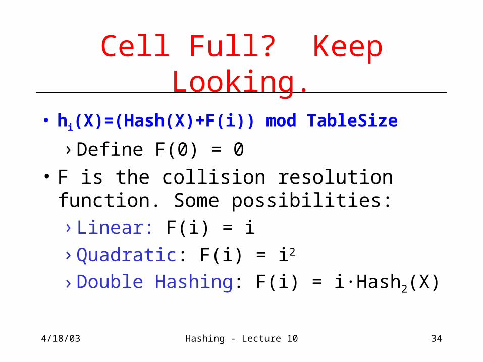
Cell Full? Keep Looking.

• hi(X)=(Hash(X)+F(i)) mod TableSize

› Define F(0) = 0

• F is the collision resolution function. Some possibilities:› Linear: F(i) = i › Quadratic: F(i) = i2

› Double Hashing: F(i) = i·Hash2(X)


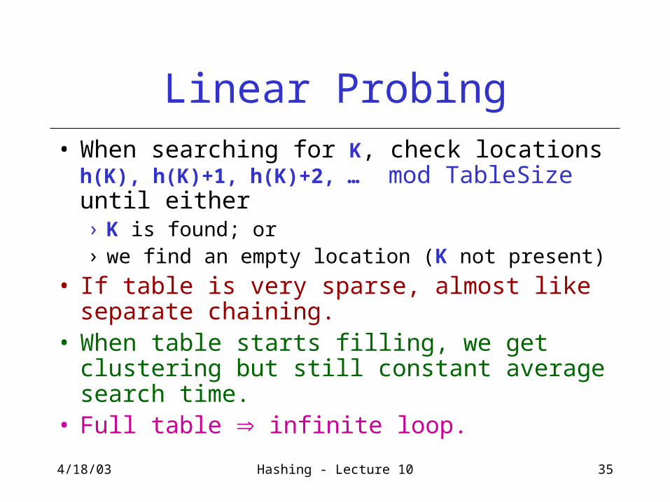
Linear Probing• When searching for K, check locations h(K), h(K)+1, h(K)+2, … mod TableSize until either› K is found; or› we find an empty location (K not present)

• If table is very sparse, almost like separate chaining.

• When table starts filling, we get clustering but still constant average search time.

• Full table infinite loop.


Primary Clustering Problem

• Once a block of a few contiguous occupied positions emerges in table, it becomes a “target” for subsequent collisions

• As clusters grow, they also merge to form larger clusters.

• Primary clustering: elements that hash to different cells probe same alternative cells


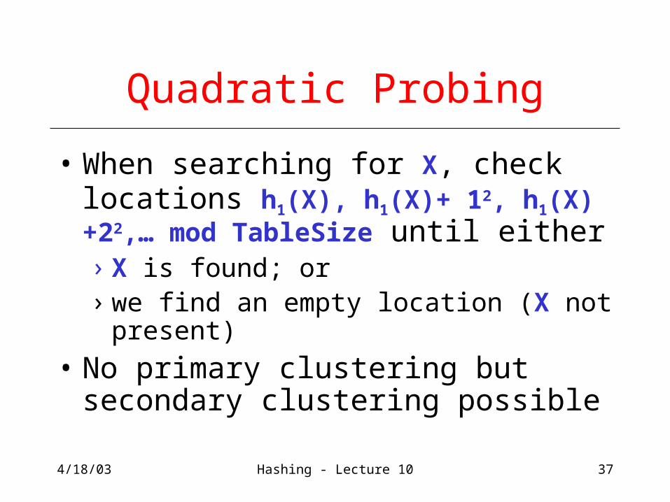
Quadratic Probing

• When searching for X, check locations h1(X), h1(X)+ 12, h1(X)+22,… mod TableSize until either› X is found; or› we find an empty location (X not present)

• No primary clustering but secondary clustering possible


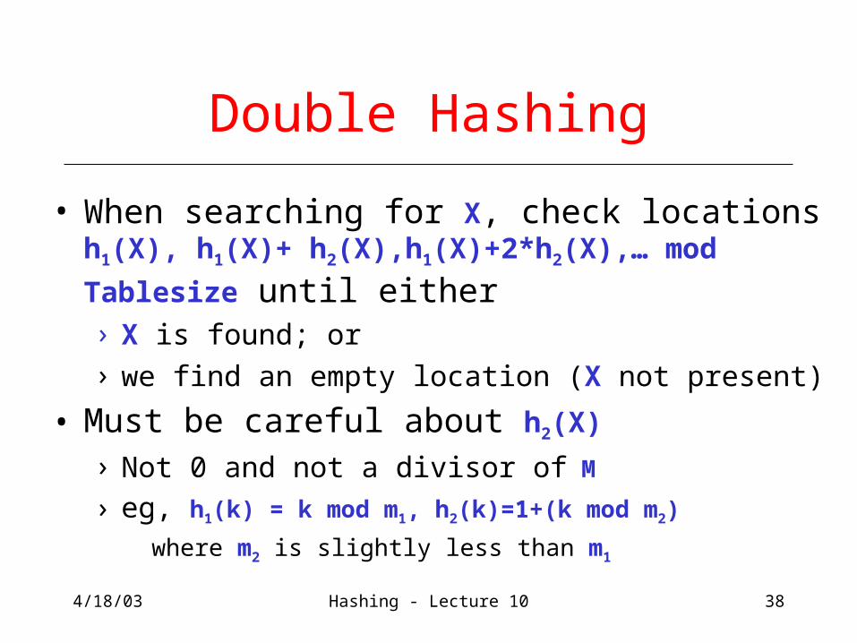
Double Hashing

• When searching for X, check locations h1(X),

h1(X)+ h2(X),h1(X)+2*h2(X),… mod Tablesize until either› X is found; or› we find an empty location (X not present)

• Must be careful about h2(X)

› Not 0 and not a divisor of M

› eg, h1(k) = k mod m1, h2(k)=1+(k mod m2)

where m2 is slightly less than m1


Rules of Thumb

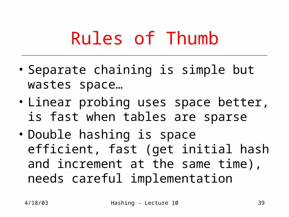
• Separate chaining is simple but wastes space…

• Linear probing uses space better, is fast when tables are sparse

• Double hashing is space efficient, fast (get initial hash and increment at the same time), needs careful implementation


Rehashing – Rebuild the Table

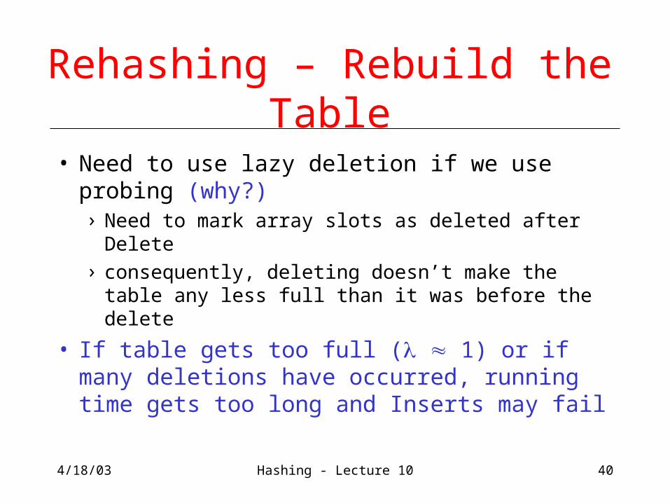
• Need to use lazy deletion if we use probing (why?)› Need to mark array slots as deleted after Delete› consequently, deleting doesn’t make the table any

less full than it was before the delete

• If table gets too full ( 1) or if many deletions have occurred, running time gets too long and Inserts may fail


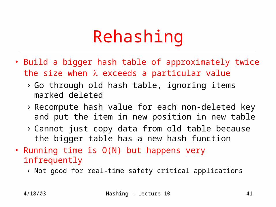
Rehashing• Build a bigger hash table of approximately twice the size

when exceeds a particular value

› Go through old hash table, ignoring items marked deleted

› Recompute hash value for each non-deleted key and put the item in new position in new table

› Cannot just copy data from old table because the bigger table has a new hash function

• Running time is O(N) but happens very infrequently› Not good for real-time safety critical applications


Rehashing Example

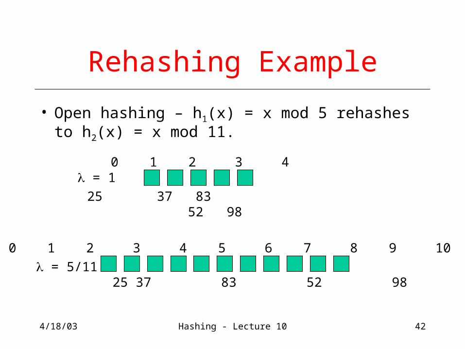
• Open hashing – h1(x) = x mod 5 rehashes to h2(x) = x mod 11.

0 1 2 3 4

25 37 83 52 98

= 1

0 1 2 3 4 5 6 7 8 9 10

25 37 83 52 98 = 5/11


Caveats

• Hash functions are very often the cause of performance bugs.

• Hash functions often make the code not portable.

• If a particular hash function behaves badly on your data, then pick another.

• Always check where the time goes

hashing cse 373 data structures lecture 10. 4/18/03hashing - lecture 102 readings reading ›chapter...

Documents

hashing lecture

hashing cse

index slide

hashing schemes

table of size

keys u

trivial slide

data structures lecture