l.IB?l\~Y STATE Or Hi·,WI-\11

DEPART~··iENT :'f PLAW-.!ING AND ECONO~ liC IJc>!ELOPMENT

r 0. Box 2359 Honolulu, Hawaii~

HA WAll DEEP WATER CABLE. PROGRAM

PHASE II-C •

TASK 4

SECOND BOTTOM ROUGHNESS SURVEY

TK3351 H35 PI IC T4 Department of Planning and Economic Development c . 1

TK:::.3S"I \I ~· ::

HAWAII DEEP WATER CABLE PROGRAM~ 1 r_;. n: ( N /. T~

"-~··' --·.- ,. ;.. ' I

PHASE II- C :) _,_, . .---

\TASK 4-

· SECOND BOTTOM ROUGHNESS SURVEY,

r.-~~~:s~t.•\RTi\.~ENT ar: PL/\t">-i:~--~ ~~- .Ji)

.cc.:ONOMIC DEVELO,'i·"·"·'··:' Prepared by P. 0. Box ~35'/,

Honolulu, Hawai; S&~04

MAKAI OCEAN ENGINEERING, INC.

and

SCRIPPS INSTITUTION OF OCEANOGRAPHY

for

Hawaiian Dredging and Construction Company

Parsons Hawaii

Hawaiian Electric Company, Inc.

and the

State of Hawaii

Department of Planning and Economic Development

MARCH 1987

CONTENTS 1.0 INTRODUCTION

1.1 The Hawaii Deep Water Cable Program 1.2 Importance of Bottom Roughness 1.3 First Bottom Roughness Cruise 1.4 Second Survey Objectives 1.5 Responsibilities

2.0 EOUIPI1ENT & METHODOLOGY 2.1 Equipment 2.2 Data Analysis

2.2.1 Purpose of Data Analysis 2.2.2 Primary Data Available 2.2.3 Data Handling 2.2.4 Data Storage

3.0 OPERATIONS

4.0 RESULTS 4.1 Data Quality 4.2 Maui Slope

4.2.1 General Description 4.2.2 Cable Path Selection 4.2.3 Photographs 4.2.4 Sea MARC Data 4.2.5 First Cruise Data, Maui Side 4.2.6 Final Maui Cable Path

4.3 Kohala Slope 4.3.1 General Description 4.3.2 Cable Path Selection 4.3.3 Photographs 4.3.4 Sea MARC Data 4.3.5 First Cruise Data, Kohala Side 4.3.6 Final Kohala Cable Path

4.4 Bottom of Channel 4.4.1 General Description & Selected 4.4.3 Sea MARC Data

4.5 Geology

5.0 CONCLUSIONS AND RECOMMENDATIONS 5.1 Route Location and Cable Laying 5.2 Survey Operations (Scripps) 5.3 Data Processing 5.4 Maui Slope 5.5 Kohala Slope 5.6 Channel Bottom 5.7 Recommendations

REFERENCES

APPENDICES A. Summary of the First Survey Cruise

1 1 2 3 4

5 6 6 6 7 9

10

14

15 16 18 18 19 19

20 21 23 24 24 25

Path 25 25 25

27 28 30 30 31 32 32

B. Plan for the Second Bottom Roughness Survey Cruise in the Alenuihaha Channel, June, 1986

C. Scientific Party and Ship's Crew D. Shore Navigation Station Locations

1.0 INTRODUCTION

1.1 HAWAII DEEP WATER CABLE PROGRAM

"The Hawaii Deep Water Cable Program is responsible for determining the feasibility of laying multiple power cables between the islands of Hawaii and Oahu in the Hawaiian Islands. One major difficulty in constructing this power cable system would be laying the cable in the very deep Alenuihaha Channel between the islands of Maui and Hawaii. This channel is 1930 m deep, has slopes approaching 30 degrees, has bottom current speeds exceeding 1 knot and the bottom in many places is extremely rough, consisting of geologically recent lava flows, benches and scarps. Because of the severity of this obstacle, a technically feasible cable path had to be found across the Alenuihaha Channel to determine the overall feasibility of connecting the islands with a power cable.

This survey, conducted from July 8 to 17, 1986, on the Scripps Institution of Oceanography's Research Vessel R/V MELVILLE, funded by the State of Hawaii. The overall Hawaii Deep Water Cable Program is supported by the Federal Department of Energy.

The preferred route for a commercial cable system from the Puna region of the island of Hawaii to Oahu is illustrated in Figure 1. The primary survey area is also indicated between the islands of Hawaii and Maui. Figure 2 is a more detailed map of the survey area in the Alenuihaha Channel. The bathymetry is based on NOAA data with the contour lines generated by the Hawaii Institute of Geophysics at the University of Hawaii. Two primary survey areas, A and B, are marked on this chart and represent the primary search areas based on the results from the first survey cruise. These are the areas where a wide, acceptable cable path was determined to be most difficult to find and where some precise commercial cable laying would probably be necessary. During a previous survey (October, 1985) the areas within the lighter A & B boxes in Figure 2 were searched.

1.2 IMPORTANCE OF BOTTOM ROUGHNESS

The cable selected in the HDWC Program is a large complex structure with a wet weight of 27.1 kg/m and a diameter of 11.8 em. This cable is to be laid on the bottom at a nominal tension (500 to 5000 kg) in order to prevent kinking during the laying process; if laid on a rough bottom the cable will be bent over obstacles and suspended between obstacles in free spans. The severity of these bends and the length of the spans is a function of the bottom roughness. The cable could be damaged during the laying process if the bend radius is less than 1.5 m, a value established by Pirelli Cable Corporation for this cable (Reference 3). Another failure mode is lead sheath fatigue caused by vortex-induced oscillations over time in the free span subjected to cross currents. Analysis by Pirelli shows that the acceptable free

0 25 50 75 KILOMETERS

100

ALENUIHAHA CHANNEL SURVEY AREA

HAWAII

GEOTHERMAJ POWER SITE

FIGURE l. PREFERRED HAWAII DEEP v/ATER CABLE ROUTE AND AREA OF DEEP WATER ROUGHNESS STUDY (REF. 7)

KILOMETERS 0 5 10

Figure 2.

ALENUIHAHA CHANNEL BOTTOM ROUGHNESS

SURVEY

HAWAII DEEP WATER CABLE PROGRAM

SURVEY AREAS

DEPTHS IN METERS

span length is a function of the cable bottom tension as follows:

Bottom Tension 5000 kg 3000 kg 1500 kg

500 kg

Maximum Span 51.0 m 40.0 m 26.3 m 17.0 m

It is necessary to lay the cable on the bottom without unacceptable spans and without unacceptable bend radii. The size of a cable span and the severity of a cable bend are functions of the bottom roughness. In order to determine the difficulty and the cost of laying the cable, the bottom roughness must be determined.

In addition to bottom roughness, other path characteristics affect the ability to lay cable. Because of the great depth and considerable currents in the Alenuihaha Channel, it is difficult to precisely lay a cable on any given path, and the degree of difficulty is obviously a function of the width and straightness of the available path. As the path becomes narrower and the radius of curvature smaller, different techniques may be required in the cable laying process and, depending upon the depth, may challenge the technical feasibility of laying the cable. Cable laying techniques are not the subject of this report. The most recent summary on the cable laying control process can be found in Reference 7.

1.3 FIRST BOTTOM ROUGHNESS CRUISE

An eight-day Bottom Roughness Cruise was performed in October/November, 1985, in the Alenuihaha Channel using the University of Hawaii's R/V MOANA WAVE and a bottom roughness survey package, "BRS", specif!.cally developed for this cruise. This survey was the first detailed look at the bottom roughness in the Alenuihaha Channel. Its purpose was to characterize the bottom roughness in terms meaningful to a commercial cable laying process. It attempted to find an acceptable cable path across the Alenuihaha Channel, identify the degree of placement accuracy required for the successful deployment of the cable, identify an optimal bottom cable tension and identify the needs for subsequent surveys. In addition to accurately measuring the bottom roughness, the first survey included operating the Sea MARC II, a wide-swath sidescan sonar system, over the area.

The primary accomplishment of the first cruise was the identification of the general level and distribution of roughness on both sides and bottom of the Alenuihaha Channel in the area of the cable route. Many major roughness concerns such as the existence of continuous and impassable escarpments or a bottom that is extremely rough everywhere were eliminated by results of the first cruise.

2

The first cruise greatly increased confidence that an acceptable cable path could be found. It was concluded that precision cable laying would probably be required during the commercial program but it would be isolated to specific locations and be a small percentage of the overall cable laying.

The first cruise also isolated the areas of concern which required more survey work, hence the second survey. Most notable of these areas of concern were the top of the Kohala slope along the 1000 m contour and between 1000 m and 1600 m along the Maui slope. Large areas of the bottom were found to be relatively easily crossed by the cable such as the very bottom of the channel and the lower portion of the slope on the Kohala side.

The first cruise did not identify a continuous path across the Alenuihaha Channel nor did it identify the width of the path in any of the areas where roughness was acceptable. Furthermore, the position of the tracks run during the survey and the position of the obstacles identified along the tracks were only known to an accuracy of approximately 150 m, unsuitable for the identification of an actual route. Appendix A is a more detailed summary of the first bottom roughness cruise.

1.4 SECOND SURVEY OBJECTIVES

The following were the goals for the second Alenuihaha Channel Bottom Roughness Survey:

1. Find the "best" path possible, for one cable, through the areas of the Alenuihaha Channel.crossing that were determined by the first cruise to be the most difficult. These areas were designated as A and B and are illustrated in Figure 2. The "best" cable path is the path with no unacceptable cable spans or cable bend radii and requiring the least difficulty for cable laying that can be found within the survey time and equipment constraints.

2. Collect sufficient data on the worst portion of the best cable route such that the cable laying requirements can be defined. Detailed bathymetric, roughness and path width information is necessary to adequately determine the required cable laying control for a commercial deployment. It was therefore a requirement of the second survey to select a cable_path such that a more concentrated data collection effort could be made along that selected path.

3. Find parallel paths for an additional two cables.

3

1.5 RESPONSIBILITIES

The following were the general responsibilities of the participants in this survey:

1. Hawaiian Dredging & Construction - HD&C had overall responsibility for the performance of the cruise including ensuring the availability of required labor, materials and equipment and the technical accuracy of all work.

2. Scripps Institution of Oceanography, La Jolla California - Scripps ISIOI had total responsibility for providing and operating the key survey equipment, most notably the Deep Tow underwater survey system and the R/V MELVILLE such that the program goals could be accomplished. SIO collected, logged and corrected all the data for this cruise and provided assistance in data interpretation.

3. Makai Ocean Engineering, Inc. - Makai performed data analysis during the cruise in order to evaluate the bottom information in terms meaningful to cable laying and helped direct the search for an acceptable cable path. Makai performed the analysis and interpretation of the data after the cruise to determine the final selected path characteristics.

4. Edward K. Noda and Associates - Noda provided Mini Ranger surface navigation and operation during the cruise and assisted Makai in the data interpretation during the cruise.

This final report is a combined effort by Makai Ocean Engineering and Scripps Institution of Oceanography. Chapter 3 on operations and section 4.5 on geology have been written by Scripps (Reference 61. The conclusions and recommendations include comments from all participants.

4

2.0 METHODOLOGY

2.1 EQUIPMENT

The key equipment used for this survey was the Scripps Institution of Oceanography Deep Tow system (Spiess and Lonsdale, 1982), a multi-sensor package towed 10 to 200 meters off the sea floor using a wire with a coaxial cable core in order that signals can be easily transmitted to the vehicle and returning data provided to the computers and displays in the laboratory in real time. This equipment has been developed by SIO and is generally used at much greater depths than the 2000 m maximum in the Alenuihaha Channel.

The Deep Tow sensors of primary importance for this operation were the narrow beam-width, 12 kHz down-looking sounder, precision quartz crystal pressure gauge, side-looking sonar (SLSl, three 35 rnrn cameras and a snapshot television. Two other subsystems on the Deep Tow played supporting roles: an up-looking echo sounder for pressure gauge calibration in terms of acoustic travel time and a 4 kHz sounder for determination of sediment thickness.

Surface navigation for the ship was provided by a Motorola Mini Ranger system with an overall accuracy of 3 m. The Mini Ranger is a microwave, line-of-sight, range-range positioning system which utilizes shore stations for positioning. Two shore stations were located on Maui at the following locations:

Location

Kahikinui

~luolea

X

190789.6 m

219737.0 m

y

31274.0 m

39543.7 m

z

439 m

98 m

These x and y locations are relative to the primary navigation grid used for both this survey and the previous survey. The grid is the u.s. Coast and Geodetic Survey Transverse Mercator for Hawaii State, Zone II, Maui. All units of measurement are in meters. The above shore stations were used for both surveys and are easily and accurately reproducible for further work. Their exact locations have not been surveyed precisely, the ab§olute position of the shore stations is within 10 meters. (see appendix D)

For underwater navigation, Scripps installed a long-based seafloor acoustic transponder grid with four bottom transponders each on the Maui side and the Kohala side of the Alenuihaha Channel. Because ship positions could be determined in both the underwater acoustic net and the surface microwave net, these dual positions could be used to fix the transponders relative to the Mini Ranger shore stations, which were taken as the primary

5

geographical reference. Periodically throughout the cruise, as more data were collected on the transponder positions, Scripps would perform an internal·"looping" process to determine the transponder positions. After the final post-expedition calculations, the RMS errors for the transponder positions were less than 5 m relative to the Mini Ranger shore stations.

2.2 DATA ANALYSIS

2.2.1 Purpose of Data Analysis

The data analysis process was developed to determine the location, if any, of a feasible path on the seafloor for a commercial cable. A feasible path is one that would not generate unacceptable spans for the cable and is sufficiently wide that one or more cables could be laid along the path. Also considered was the cable turning radius which, at the start of the cruise, it was desired to keep at 1 km or greater.

Data analysis was performed onboard during the cruise to identify as quickly as possible potential cable paths in order to help direct the search effort. It was therefore necessary to develop techniques that would quickly recognize an unacceptable cable path.

2.2.2 Primary Data Available

The key data that were available for determining cable path suitability were detailed bottom profiles, sidescan images, and bottom photographs all with accurate bottom positioning through the two navigation grids. All the data, with the exception of bhe photographs, were available in real time.

The bottom profiles were obtained by adding the pressure signal from the quartz crystal pressure gauge on the Deep Tow package with the down-looking sounder. The intent was to achieve a very high resolution profile of the bottom roughness (15 em or better (See Section 4.1). These data were the only means of quantitatively evaluating bottom roughness and determining whether the bottom was suitable for a cable. These data did not, however, yield any information relative to path width except by comparing cross and parallel Deep Tow tracks.

The sidescan data from the Deep Tow provided qualitative information on the bottom roughness approximately 300 to 450 meters to either side of the vehicle. It was only possible to "calibrate" the roughness observed by comparing parallel and cross tracks of the Deep Tow and looking at the detailed bathymetry and sidescan at identical locations. This normally could be quite easily accomplished because of the excellent navigation on the Deep Tow package.

The navigation data consisted of a real time plot of the Deep Tow position with a new position determined every 5 minutes. The

6

sidescan, bathymetry and photographs were all marked with an identical time base such that it was fairly easy to cross reference the available data.

Photographs were taken of the bottom on designated "camera runs". For a camera run, the Deep Tow would be flown 10 meters off the sea floor and the winch operator would key the camera shots. The photographs would view an area approximately 5 meters by 7 meters on the bottom and were valuable in obtaining a knowledge of the texture and makeup of the seafloor. This information was not easily discernible from the sidescan or detailed bottom bathymetry data. The photographs alone, however, did not provide sufficient information relative to overall roughness and potential cable spans; the scale was too small. Unfortunately, the higher frequency pinging rate for flying the Deep Tow close to the bottom to make the camera runs interfered with the detailed bottom bathymetry data.

2.2.3 Data Handling

The sidescan, the detailed bottom bathymetry and the Deep Tow position were plotted in real time (Deep Tow position would be uncorrected and later repositioned as bottom transponder locations were corrected). After a few hours delay, Scripps personnel would combine electronically the bottom data with the navigational positioning and transfer these combined files to the data analysis computers. The data analysis computer work would consist primarily of looking for bottom roughness that would cause an unacceptable cable span if the HDWC cable were laid along that particular Deep Tow track.

Based on this preliminary cable span analysis, hand-drawn mosaics of th~ sidescan records and manual interpretation of the high resolution bathymetry tracks, it was possible to piece together an entire picture of the bottom that was sufficiently accurate and detailed to direct the cruise search.

7

After the cruise, the bottom navigation data were re-analyzed by Scripps and corrections made, as necessary. This was particularly important for the Kohala slope area where the acoustic navigation was intermittent due to the large irregular topography on the bottom. After the cruise, these new navigation data were again combined with the precise bottom bathymetry and re-analyzed for bottom spans. Because at this point the search for a cable path had already concentrated on particular areas on the Kohala and Maui slopes, the analysis that was performed after the cruise concentrated in these areas.

The final measure of impact of bottom roughness on a commercial cable deployment was determined by analytically laying a cable over the measured profiles and computing the lengths of the resultant free spans and the associated bend radii. Because of the very large quantity of data gathered for determining the bottom roughness and because only the more elevated data points affect the cable shape and spans, the cable program makes successive approximations of spans before utilizing a detailed analytic cable solution.

The first approximation can be visualized as rolling a ball along the bottom roughness data. The first approximation of cable contact points is made when the ball contacts two data points. The ball is 'rolled' one more step to get an approximation fer the next span, which is used in determining an approximate end condition for the current one. A more exact solution for the span is then calculated, knowing the span length and the approximate cable angle at each of the contact points. This more exact solution is compared to the bottom bathymetry between the contact points to ensure that it is indeed a valid cable span. If not, new intermediate contact points are determined and the process is re~eated. Once a clear span is determined, the bend radius at either end of the span is also computed. If the span is of excessive length, as determined by Pirelli's criteria for critical span length as a function of the laying tension, it is tabulated as an unacceptable or critical span. If the bend radius is less than 1.5 m, it is also tabulated as an unacceptable span for reasons of bend radii.

This analysis gives an estimation of cable touchdown points and subsequently, spans and bend radii, based primarily on Love's equation (Reference 4l. This method, although complex, is only an approximate solution to the differential equations modeling a laid cable. A comparison of selected analytic results with scale model predictions are given in the First Bottom Roughness Survey Report (Reference 5) .

Figure 3 illustrates spans for a cable laid along a typical section of bottom roughness profile at 3000 kg bottom tension. The raised line is a representation of the cable (straight lines) elevated slightly above the bottom for clarity. The higher tensions give slightly longer spans, often contacting different end points than the lower tensions. Figure 4 is an illustration of a

8

200M

Figure 3. Representation of cable spans over a rough bottom,

cable laid at 3000 kg.

,- - -

------- ·-· --

' I

I AO.T3 I

v4.-T2

~ 5.-Tl 51.-T3

I

Figure 4.

.

~

-I ~

I

Multiple unacceptable cable spans computed along Maui Track at different laying tensions.

l

1200

I I I '

1300 I

1400

I I

I I

--L--_j

track on the Maui side between 1300 m and 1400 m depth with multiple spans at different tensions. The span locations, lengths and tensions are graphically shown; only the spans which are unacceptable based on Pirelli's criteria are shown.

2.2.4 Data Storage

All the recorded data, with the exception of the photographs, have been electronically stored. The sidescan data have been digitized and are stored at Scripps. The navigational data for all the tracks and the detailed bathymetric data are available both on 9-track tape and double-sided, double-density 360K diskettes. For all the tracks where there was good bottom navigation, the bathymetry and position data have been combined. These data are available both at Scripps and Makai Ocean Engineering.

Three cameras on the Deep Tow took simultaneous photographs, 733 photographs for each camera. The negatives for two of the cameras are stored at Scripps, the third at Makai Ocean Engineering. Several representative photographs are included in this report.

9

3.0 OPERATION (Scripps Institution of Oceanography)

The R/V MELVILLE arrived in Hilo at noon (GMT +10) on 8 JulY, 1986, with all Deep Tow equipment on board and checked oJt. The. Hini Ranger antenna was installed, computers to be used by Noda and Van Ryzin were set up in the upper laboratory, and cables were run to connect them with the Deep Tow computers in the main lab two decks below. During this period a Coast Guard officer was interviewing members of the crew and scientific party in connection with an accident which had occurred three days before. Upon completion of the Coast Guard inquiries and initial checkout of the data processing and Mini Ranger systems we sailed from Hilo at 2000. The scientific party consisted of 15 from SIO and 4 associated with HD&C, with F. N. Spiess as Chief Scientist and 22 crew under C. Johnson, master. A full list of participants is given in Appendix C.

At 0330, 9 July, we were in the survey area and established a real time plot of the ship's track based on Mini Ranger data. We then started maneuvering to launch transponders. Our plan was to use two sets of four units each, in approximately square arrays 4 km on a side, one on the Maui slope and the other on the Kohala (Hawaii) slope, with about 5 km between their edges. The arrays were located to give the best possible coverage of the zones pictured as optimal in Figure 41 of the First Cruise Report, Reference 5. Sound propagation calculations based on temperature profiles provided by Noda, and the bottom topographic profiles obtained from Bottom Roughness Sampler data contained in Reference 5, showed that the usefulness of the shallower transponder pair on the Kohala slope would be related to placement relative to the sharp slope change at about 950 m depth. As the actual location of that break was not well established in Mini Ranger coordinates, we decided to place the other six units and then put in the southernmost pair when we had a better understanding of the area.

The first transponder was launched on the Maui side at 0443, July 9 and the sixth at 0834. Three of these units had current meters attached in order to provide environmental information for correction of transponder navigation, if necessary.

At 0905 Deep tow fish number 5 was launched and the first of three lowerings commenced. Our plan was to make initial passes parallel to the contours near the slope break on the Kohala slope in hopes of finding indications of an optimal track and of relating the larger scale SeaMARC 2 images to the Mini Ranger coordinate system. After two such passes it became clear that time would be required to assimilate the SLS data and that a full scale operation on the Kohala side should await installation of the upslope transponder pair. We thus decided at about 1700 to make a run downhill approximately along one of the lines suggested in Reference 5 as a potential route and up on the Maui side. During this run it was found that the transducer

10

orientation arrangement for our precision sounder was not performing adequately and depth data were being unacceptably degraded. We thus used the uphill Maui-side run as a reconnaissance pass and at the uphill end brought the vehicle on deck, terminating lowering one at 2337 on 9 July.

After altering the transducer mounting arrangement to fix the unit to the vehicle, and repairing a bad spot in the main signal and power lead at the fish slip range, the vehicle was back in the water at 0210, 10 July, starting lowering two, concentrating on the Maui side.

Given the patchy appearance of the Sea~ARC imagery on the Maui side, the irregular distribution of unsatisfactory spans in the BRS data and the rather uniform nature of the slope, we decided to make a series of uphill/downhill runs to see the nature of the topographic profiles as well as to develop SLS images which might assist both in finding useful routes and in matching up with the SeaMARC images.

After making 5 such runs, spaced about 1 km apart, it began to appear that there was a very rough zone between about 1050 and 1250 m depth, as well as scattered blockages somewhat deeper. In order to assess the continuity of the 1050-1250 barrier we then made two runs (between 2030/10 and 0200/11 July) parallel to the contours just at the lower and upper edges of that zone. This confirmed its continuity, although there was some suggestion of its being subdued in the vicinity of the northeast transponder.

By this time the post-processing data analysis team (Van Ryzin, Noda, Linzer and Walsh) had begun to develop a comprehensive picture and we made a run starting at the downhill edge, along the potential cable route but swinging to the north through the subdued zone and up to the 800 m contour. Although this path had several unsatisfactory sections, it did look promising in the 1050-1200 band.

We then made a downslope run to the east of the previous tracks, an upslope one close to the original poor data pass of lowering one and a downslope run west of the previous coverage, all confirming the bad terrain in the 1050-1250 depth range.

At about mid-day on 11 July we were informed that Frank McHale, the HD&C representative on board, would have to go ashore in the next day or so. We thus laid a plan to work farther to the east on the Maui slope and then to pull up the vehicle and head for the north end of Hawaii to transfer him to a boat arranged by Ed Noda.

We then went back through the central area in a northeasterly direction. This run began to provide indications of possible satisfactory links to good portions of other tracks. We.then made a

11

downslope run 3 km east of our previous coverage. This showed that the bad mid-depth band did not extend that far, although there was other rough topography at the deep (1600-1700 ml end of that track. We followed with a set of upslope, downslope tracks to f"ill the space between the new one and the solid coverage to the west, determining the end point of the 1050~1250 rough zone and finally making a.photo run down the slope to terminate lowering two at 0730 local time on 12 July after 53 hours of continuous towing.

Since we now had substantial coverage on the Maui side our plan was to steam south to effect the personnel transfer and then return to the Kohala slope, install the originally planned final two transponders, and work on that area for several days. This we did, launching the seventh and eighth transponders at 1200 and 1238 (local time) respectively and starting lowering number three at 1330 on that day (12 July).

The initial passes "parallel to the contour lines" had shown that the slope below the shelf break was gullied - i.e. the contour lines were not as simple as shown on the base charts displayed in the May 1 report. This substantially reduced the effectiveness of across slope runs. Given the insights gained from successive up and down slope runs on the Maui side we decided to use this method on the Kohala slope as well, emphasizing the interval from 900-1500 m in depth. Below 1500 m both our scattered runs and the earlier BRS data showed benign topography.

After 10 passes (mostly done as downhill runs, pulling up and returning high off the bottom to avoid having to go up in close contact with the very steep portions of the slope) , a consistent picture emerged in which there were several marginal paths over the slope break, but backed on the shallow side by forbidding rough lava flow zones. One acceptable path straight downhill was found, by working from adjacent SLS images, and, following the texture implied by the SLS data, a second good path slanting downhill from SW to NE was also mapped out. Both of these were backed on the shallow side by a smooth zone with rippled sediment cover, probably sand. At this point our tactics changed and we made two camera runs and additional profiles close to the two good paths to verify that the gaps were at least 100 m wide.

With satisfactory results on the Kohala slope (by 0200 local time on 15 July) we returned across the channel axis to the Maui side, starting at the eastern end of the previously surveyed zone. There we found unsatisfactory roughness near the bottom of the slope (1600 ml which marred our optimism about that region.

The data processing group had by then gone over the data from the July 10-12 period and found several track segments which seemed to link together to make a satisfactory path, although the SLS data indicated only a rather narrow pass through the rough 1050-1250 meter zone. We thus laid a set of tracks to verify that this path existed and to put limits on how sharply curved the various

12

sections would have to be. At this stage of our data reduction it appeared that the narrow gap available at about the 1100 m level was about 80 m wide and that the turn to the west at the shallow end could be made with about a 1 km radius. The shallow end was pursued satisfactorily to the west to the limit of Mini Ranger coverage at about the 500 m contour. This phase was terminated with a camera run down through the narrow gap, ending on the afternoon of 16 July.

With some time left before the transponder recovery operations planned for early daylight on 17 July we decided to make a swing to the vest to put some limits on the mid-depth rough topography band. This took us 3 km farther than any of the previous tracks and we still encountered a zone with -unacceptable topography.

The fish was brought on board at 0443 local time the morning of the 17th and transponder recovery operations began at first light. All eight units were recovered by 0940 and the ship headed for Hilo, arriving at 1700 to disembark the scientific party and off load the Mini Ranger and the post-processing computers.

13

4.0 RESULTS

4.1 DATA QUALITY

The sidescan data proved to be extremely valuable, qualitatively showing targets out to 450 m to either side of the vehicle. The extent of this coverage depended upon the bottom roughness and the height of the vehicle off the bottom. Because of the frequent time marks on the sidescan record and the accurate Deep Tow bottom navigation, sidescan images could be matched quite accurately.

The only sidescan data that were difficult to interpret were the images for the steep Kohala slope. For this slope the record had a very high contrast and individual targets and roughness was difficult to identify. Large features, however, on the Kohala slope could be easily seen.

In order to properly evaluate the effect of sea floor roughness on the submarine cable, an attempt was made to measure the bottom bathymetry to a resolution of 15 em. This was not achieved on this cruise, particularly in rough regions. Figure 5 illustrates a typical record from the pressure plus downward­looking sounder (pressure plus down) data. The horizontal lines are spaced at 100 m and the illustration shows both a portion of the smooth and rough bottom. The smooth area is shown to be relatively flat with a few "holes" in the data. The rough areas are seen to be quite jagged and not a very realistic representation of a rough bottom •. The rapid amplitude variations from point to point are incompatible with the cone angle and sample area of the down-looking sounder. Similar rocky areas surveyed with the bottom roughness sampler during the first cruise yielded results which looked quite different and less jagged.

The bathymetry data were therefore carefully checked manually both before and after the computer span analysis. It was necessary to eliminate data spikes that would either cause or prevent a cable span from occurring. Once these .manual checks were performed, the detailed bottom bathymetry proved to be quite useful. Most spans were caused not by individual rocks or roughness but by larger scale variations in the bathymetry. In addition; the path selection process always favored selecting a path which had a smooth bottom, as seen to the right of Figure 5. Rough areas, clearly identified by the bathymetry record, were thus avoided.

It is difficult to determine the final resolution of the bathymetry. In the smooth areas, resolution is probably within the 15 em originally desired. In rough areas, the resolution is probably not within 1 meter. Although this is less accurate than the original bathymetric system design called for, in hindsight it was adequate. Since the vast majority of the selected path was over a smooth bottom, the lack of precision on a rough bottom did not compromise the final results. On the small portion of the

14

Figure 5.

·---------------,

57.- T 4

Typical bottom data from deep tow with computer generated cable spans shown.

selected path that crossed a rough bottom, there are identical survey tracks from both the previous survey (with 15 em resolution) and the present survey. The data from both surveys yielded identical unacceptable span results. The overall bathymetric accuracy agrees extremely well for cross and parallel tracks and also agrees extremely well with data from the previous bottom roughness cruise. All cross referencing of bathymetric data had agreement to within 5 m.

While building up the data summary charts on both the Maui and Kohala sides of the channel, it was possible to check the accuracy of the Deep Tow positioning. Specific targets could be identified and positioned from parallel and cross sidescan records. On the Maui side, cross referencing speciric targets proved to be quite accurate. On the Kohala side, however, there were errors of up to 30 m for some specific targets. Throughout the cruise, the Kohala side was difficult from the navigation point of view because of the rough terrain and the Deep Tow would frequently loose contact with the bottom transponders.

4. 2. MAUI SLOPE

4.2.1 Description

Figure 6 shows the planned survey area and all the tracks of the Deep Tow on the Maui side of the channel. Because of the complexity of this side of the channel, the survey concentrated in this area. Approximately 100 square km was covered in detail varying in depth from 1930 m to 430 m. Over 100 hours of Deep Tow bottom data were gathered.

As determined on the first survey cruise, the Maui slope proved to be quite complex with many rocky escarpments resulting either from old shorelines, debris flows, faults or lava flows. Figure 7 illustrates the overall Maui slope with the rocky areas highlighted as determined from both the sidescan and the bathymetric records. The illustration is oriented with North to the top and horizontal and vertical axes are marked at 1 km increments; the axes values refer to the Hawaii State Grid, Zone II. Superimposed on this illustration are many of the Deep Tow and the previous cruise BRS tracks with the locations of computed unacceptable spans. Figure 8 is an enlargement centered on the more probable path area.

The data shown in Figures 7 and 8 were independently gathered from the sidescan and bottom roughness span analysis. The rocky areas are primarily the interpretation of many sidescan tracks and the span positions are determined by computer runs of the bottom roughness data. In most cases, there is excellent agreement between the detected spans and rough areas with the exception of some of the data that were collected during the first cruise which had no bottom positioning capability.

15

w 0 0 0 0

N '-" 0 0 0

N 0 0 0 0

210000 215000

Figure 6. All Deep Tow Survey Tracks on the Maui Slope Together With the Planned Survey Area.

220000

w 0 0 0 0

N V' o­o 0

N 0 0-0 0

UNACCEPTABLE SPANS

0 500 KG TENSION

L'J 1500 KG TENSION

0 3000 KG TENSION

0 5000 KG TENSION

205000 Figure 7.

210000 ' 215000 22oboo .I

Maui Slope Showing Both Deep Tow Tracks & First Cruise Tracks With Resulting Computed Unacceptable Cable Spans & Rocky Areas Shown.

0

210000 I

212000

Figure 8. Enlargement of Figure 7, Centered About Primary Search Area.

1500 KG TENSION

3000 KG TENSION

5000 KG TENSION

I 218000

The bathymetry in Figures 7 and 8 is derived from the Deep Tow tracks by simply connecting common depths along the track profiles. The bathymetry is therefore better known in the area of concentrated Deep Tow study.

!-Tell illustrated in Figures 7 and 8 are several difficult areas for the potential cable system. In a wide band from 1100 m to 1250 m is a series of very rocky and rough terraces that were very difficult to work through. Several Deep Tow passes far to the east and far to the west searched for a path through this region. These terraces disappear far to the east but the region just below this is quite rough. Other difficult regions to cross were at 1350 m and again at 1530 m where nearly every track showed a small escarpment of 5 to 20 m.

Figure 9 is a photo mosaic prepared by Scripps of the central portion of the Maui slope that is illustrated in Figure 8. The best side scan image is.obtained by looking at multiple passes of the same object. The central white line is along the Deep Tow track. Dark areas are high acoustic reflections and light areas are shadows. The rough region between 27000 N and 28000 N can be seen.

Figure 10 illustrates the typical terraced area on the Maui slope between 1100 and 1300 m. The vertical grid spacing is 100 m. In nearly all cases, crossing this region results in unacceptable cable spans for multiple cable laying tensions, in this case 1500 to 5000 kg.

4.2.2 Cable Path Selection

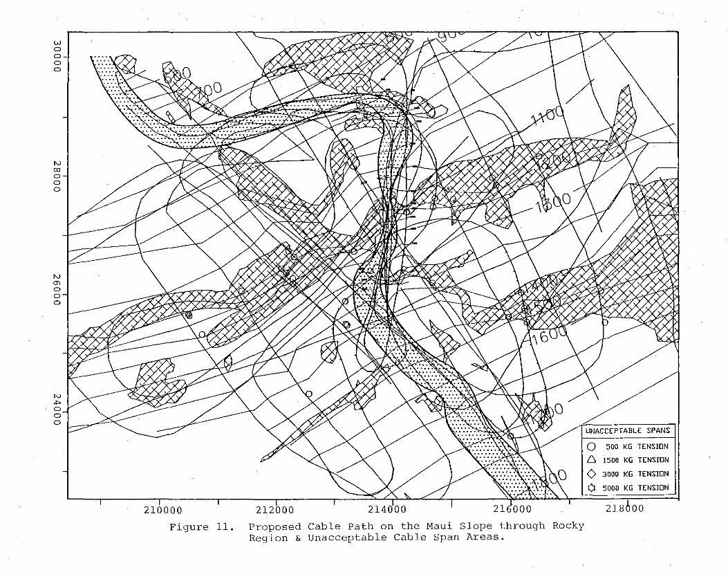
Figure 11 illustrates the position of the selected cable path on the Maui side. This path goes through the only passage that was found in the 1100 to 1250 m depth region. This is the most formidable obstacle to laying the cable across the Alenuihaha channel; an enlargement of this area is shown in Figure 12. The width of this pass is 80 m with rock outcroppings on either side approximately 4 m high. The bottom is smooth and sandy with a few small rocks 30 to 40 em in size at the base of the ledge on the eastern side (as seen in photographs). Note that one track passed successfully over the rock ledge on the eastern side without generating any cable spans; this success was due primarily to the narrow angle between the Deep Tow track and the face of the ledge. Any tracks to the right or left of this path resulted in multiple spans and the sidescan images show considerable roughness in these regions.

Figure 13 is a sidescan image of the narrow pass illustrated in Figure 12. This sidescan is a blown-up portion of the sidescan mosaic seen in Figure 9 but is also a negative of that image. The negative is more "natural" for viewing because shadows are portrayed as black regions and the light regions are those with high acoustic reflections. The white line in the illustration is

16

Figure 9. Side Scan (Scripps) Mosaic of Maui Slope Concentrating in Cable Path Area.

llOO

~~6.:iP -r~ -11

1200

~1.-T3

1300 I

Figure 10. BRS Profile of Typical Region 1100 m and 1300 m on the Maui Slope.

w~--~--~~~~~~~~~~J<--1 0 0 0 0

"' co 0 0 0

210000 212 00

Figure ll. Proposed Cable Path on the Maui Slope through Rocky Region & Unacceptable Cable Span Areas.

0 !::, 1500 KG TENSION

() 3000 KG TENSION

Q 5000 KG TENSION

218 00

213000 214000

UNACCEPTABLE SPANS

0 500

6 1500

<> 3000

0 5000

/

21'sooo

KG

KG

KG

KG

TENSJDN

TENSJDN

--·-I

216000

Figure 12. Details of Proposed Maui Path in the Narrowest Region at 1100 m to 1250 m Depth.

0 0 0 r-

"'

Figure 13. Inverse Enlargement of Side Scan at Narrowest Portion of Path. (80 m width) Cable Path is Shown; Downhill to Right.

the proposed cable path, passing between the two obstacles at the center of the photograph. The black line to the left of the cable path is the Deep Tow track for this particular track. The bottom roughness analysis generated multiple spans along this Deep Tow track near the middle of the photograph. This span analysis together with parallel Deep Tow sidescan records show that the obstacles in the middle of the photograph are not isolated but tied into more formidable obstacles both to the right and the left of the selected cable path.

The area below 1200 m opens to a wide sandy region and the cable path can widen considerably. At 1350 m directly below the pass is another shelf which must be avoided by moving to the west. This region is illustrated in Figure 14. Once past this obstacle at 1350 m, the recommended path moves toward the southeast along multiple successful BRS and Deep Tow bottom tracks. A more gentle curve was not possible at the 1400 m depth because of a ledge tha~ was observed at 1530 m crossed by multiple Deep Tow tracks just to the west of the proposed path.

Several spans are indicated in the middle of the selected cable route at 1325 m and at 1400 m depth (Figures 12 and 14). These were observed from Deep Tow tracks going across the planned route and are the result of a well rounded and smooth "hill" running almost parallel with the proposed route. It is not expected to cause problems with a cable layed along the path.

At 1525 m a rubble area stretches across the path (Figure 14) but generates no spans in six individual survey track crossings. It is small and does not cause any concern.

The region just to the north of the 1200 m deep path is illustrated in Figure 15. In this region the path must turn abruptly to avoid an extremely rough region in the 800 to 1000 m depth range. To make this bend, the cables need to be laid along the recommended path at approximately a 0. 5 to 0. 7 km radius. !A7hen the path is nearly parallel to the 900 m contour, an additional path restriction occurs which is 170 m wide. Moving uphill from that point, the path width greatly increases and stops at 500 m depth which was the extent of this survey. Only one survey track was made in this shallower region, beyond the test plan. There may well be alternate paths toward the Maui cable landing.

A possible alternate path near Maui was discovered during the post analysis and can be seen in Figure 15. An acceptable path may well be possible below the rocks just south of the cable path bend. This would enable the cable to be laid at a much more gentle radius on the bottom but the data from this cruise are insufficient to prove that this is a viable path.

Some BRS and Deep Tow tracks did cross rough regions without generating spans if the cable laying tension was as low as 500 or 1500 kg (Figure 16). While it may be possible to lay the cable at

17

UNACCEPTABLE SPANS

0 500 KG TENSJON

1275 C::, 1500 KG TENSrDN

0 3000 KG TENS JON

¢ 5000 KG

2l4ooo Figure 14. Details of Proposed Maui Path Below 1250 M.

0 0

-o r-N

0 0 0

"' N

UNACCEPTABLE SPANS

0 500 KG TENSlDN

C:, 1500 KG TENS !ON

0 3000 KG TENSlDN

0 . 5000 KG TENSlDN

N

~ CD 0 0 0

'

212000 213000 214000

Figure 15. Details of Proposed Maui Path Above 1100 M.

0 500

C:, 1500

0 3000

0 5000

KG

KG TENSION

KG TENSJDN

KG TENS JON

212000

Figure 16.

214000 216000

Computed Unacceptable Cable Spans at 1500-500 kg Laying Tension only, on the Maui Slope.

low tensions across this region, there are really no assurances and it was impossible to determine from the sidescan image how wide the path is for laying at 500 kg bottom tension. When laying cable over a very rough bottom, the generation of an unacceptable span is almost a random occurrence. Therefore, crossing ·a very rough region at a low tension would always be associated with some probability of generating an unacceptable span. As a result, only a path with a smooth bottom was deemed acceptable for this program.

For the narrow pass illustrated in Figure 12, a cable could be laid at any tension from 500 to 5000 kg without risk of causing an unacceptable span. It is recommended, however, that the cable tensions be kept as low as possible in the event of"missing a span and laying over the rocks to the left or right of the pass. At low tension, there is a much lower probability of creating an unacceptable span than at higher tensions. The maximum tension should stay at 3000 kg or less to be conservative.

4.2.3 Photographs, Maui Side

One photographic run was made of the 11aui side directly down the proposed cable path. Figure 17 shows the track of the Deep Tow while it was photographing the bottom. Along this track, spanning the depths from 1100 m to 1400 m, Deep Tow took 270 photographs from a distance of 10 m off the bottom. Several representative photos are shown in Figure 18 and their location relative to the cable path is illustrated in Figure 17. Photograph A is typical of the sediment covered bottom and is typical of most of the cable path. The Deep Tow vehicle was moving toward the right and is approximately 10 m off the bottom. The bright object to the left in each of the photographs is the flash which hangs on a cable approximately 8 m below the Deep Tow system. By this means, Scripps is able to show more texture in the bottom photographs. The area of the bottom illustrated is approximately 5 m by 7 m.

Photo B in Figure 18 was taken immediately on the edge of the narrow portion of the cable path at approximately 1160 m depth. Deep Tow was moving down the slope, to the right in the photograph. The number at the bottom of the photograph is the time of day: 22 hours, 42.23 minutes.

Photo C in Figure 18 is typical of the central portion of the narrow pass at 1190 m; one rock approximately 30 to 40 em in diameter is shown.

Photo D in Figure 17 is not on the cable path but represents the face of the escarpment in 1350 m that the cable path avoids. From the photograph, the well-rounded and worn rocks appear unstable but yet at the base of the ledge there is no talus slope and very few rocks are on the sediment base. Figure 19 illustrates the profile of this slope with the very abrupt termination of rocks at the base. This slope would generate unacceptable spans at 3000 and 5000 kg but none at 500 or 1500 kg. It was decided to preferably lay the cable to the west of this obstacle.

18

/

/

,/ /

/ //

'

c

••• 0 ••••••••••••• ·.•

••••••••••••••• 0 •••••

~---1250

______ 1275

214000 215000

Figure 17. Photographed Areas on the Maui Slope. Complete Photo Coverage for Track Shown; Specific Photos Shown in Fig. 18.

0 0 0 \!)

N

A. 1135 m, Along Path. 213981 E, 27875 N

C. 1190 m, Along Path, Center Narrowest Portion. 213940 E, 27519 N

B. 1170 m. Edge Cable Path in Narrowest Portion. 213959 E, 27663 N

D. 1350 m, Off Path, Middle Rough Slope. 213896 E, 26245 N

Figure 18. Bottom Photographs, Maui Slope

I

' ?" /' I

... ·----------~ -----~-~---··

I I I I ' ")" /'

I ,)

~ ~

I !_ /' /'

f-

~

... - ---·

Figure 19. Profile of escarpment seen in photograph 17-D. From Deep Tow data.

4.2.4 Sea MARC Data

Several cruises have been conducted in the Alenuihaha Channel by the Hawaii Institute of Geophysics, University of Hawaii, utilizing the Sea ~ARC II sidescan system. This low-frequency, shallow-towed sidescan system maps a swath many kilometers wide on the seafloor. Figure 20 illustrates the Sea .~ARC data for the entire channel crossing with the approximate location of the proposed path superimposed. The Sea MARC data were not corrected for depth variations nor were positions accurately determined during the survey. Once the Sea MARC data were oriented relative to the obstacles observed by the Deep Tow system, they proved to be quite valuable for determining an overall picture of the features both on the Maui and Kohala sides of the Alenuihaha Channel.

This Sea MARC image was available prior to the first survey cruise but only some pf the lava flows on the Kohala side could be identified and related to the BRS bathymetry data. The Maui side was difficult to orient relative to the BRS data. With the Deep Tow data, the Sea MARC information became much more meaningful and it was possible to position the cable path as shown.

One misleading feature of the Sea ~ARC data occurs on the Maui side just below the portion of the cable path running parallel to the contours. The very dark return of an image just below this portion of the path seems to have obscured and lightened the images immediately below in the 1100 to 1250 m depth range. During the first cruise, many attempts were made to cross this apparently "clear" area without success. The Deep Tow sidescan subsequently showed that this was a rough series of terraces with the exception of the one narrow pass discussed above.

4.2.5 First Cruise Data, Maui Side

With the first bottom roughness cruise, without the benefit of sidescan, it was determined correctly that there·were a wide number and wide scattering of unacceptable rough areas on the Maui side, that the most difficult area would be in the 1100 to 1600 m depth range, but no overall understanding of the nature of the slope was possible. For the second cruise, the BRS tracks and computed spans proved to be valuable in guiding the Deep Tow tracks and in finding one acceptable path into the shallow 500 m depth waters.

4.2.6 Final Maui Cable Path

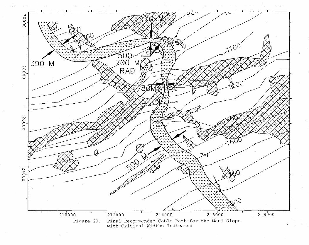
Figure 21 illustrates the final path selected along the Maui side. The narrowest portion is at 1200 m depth and is 80 m wide with a smooth bottom. The second narrowest portion is at 900 m depth and is 170 m wide. All other portions of the path are considerably wider, up to 500 m wide. The one severe bend in the cable path at 1000 m depth has approximately a 500 m to 700 m bend radius. Figure 22 is a composite profile of the path selected based on multiple Deep Tow tracks. It is not distorted, the slopes

19

Figure 20. Sea MARC II Data--Hawaii Institute of Geophysics. Alenuihaha Channel with Channel Crossing Superimposed.

N 00 0 0 0

N

"' 0 0 0

N , 0 0 0

210000 212000 214000 216000 Figure 21. Final Recommended Cable Path for the Maui Slope

with Critical Widths Indicated

218 00

0

00 HD\o. c Cf BLE RDU, E PF DFIL [---'~

~00 MAU SID 1-) t-

tJoo

14oo

t;oo -........___

00

1--700

~00

l9oo

000

1100

1200

300

400

500

600

700 .

1800

900

12ooo .

Figure 22. Profile Along the Recommended Maui Cable Path.

are accurate; the profile is folded to show 12 km of the seafloor along the selected path. The bottom is smooth and the cable could be laid at any tension up to 5000 kg without generating any unacceptable spans, although lower tensions are recommended (3000 kg or less) •

4.3 KOHALA SLOPE

4.3.1 General Description

Figure 23 illustrates the planned survey area for the Kohala slope and all the Deep Tow tracks. Sixteen square kilometers were surveyed on the Kohala side, -ranging in depth from 880 m to 1930 m, the bottom of the Alenuihaha Channel. The search area concentrated about the top of the Kohala Slope, at approximately 1000 m, which had been identified in the first survey as being the most difficult area to cross.

The Kohala side of the channel is distinctly different from the Maui side. The major feature is one very steep slope, approaching 30 degrees, dropping from 930 m to 1930 m. In the areas searched, there are no terraces and benches which were the predominant feature on the Kohala side.

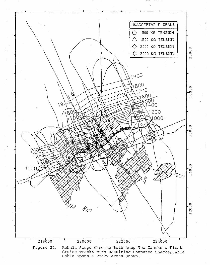
The primary features observed on the Kohala slope are illustrated in Figure 24. At the top of the slope (bottom of the page), the seafloor is quite flat with a slope of less than 1 degree in most areas. The heavy line illustrated in Figure 24 is the top of the slope and varies in depth from 920 m to 960 m. The rocky areas shown in this figure are the combined product of the Deep Tow sidescan, the detailed Deep Tow bathymetry and the Sea MARC II sidescan. Near the center of the illustration a hatched area with + signs indicates rubble areas which are difficult to define from the sidescan image.

Figure 24 shows all the survey tracks that have been made on the north Kohala slope during both the first and second cruises. Also shown are the computed unacceptable span locations for the tracks that were visually observed to have some potential as a viable cable path. Most of the tracks could be dismissed as potential cable paths by simply observing the bathymetric data.

Two major areas of difficulty were observed along the Kohala slope. The top edge of the slope from 950 to 1200 m was observed both in the first survey and confirmed in the second survey to always be rough no matter what track was analyzed. Secondly, there are several distinct lava flows at the top of the slope which greatly restrict the cable in this area. These lava flows are shown in Figure 24 and also easily seen in the Sea MARC data in Figure 20.

A Deep Tow sidescan mosaic prepared by SIO is illustrated in Figure 25. This mosaic concentrates on the central portion of the

20

217000

oo

220000 225000

Figure 23. All Deep Tow Survey Tracks on the Kohala Slope Together with the Planned Survey Area.

0 0 0

"' N

0 0 0 0

"'

0 0 0 L1l r-l

0 0 0 r-l ,...;

UNACCEPTABLE SPANS

0 500 KG TENSION

[':, 1500 KG TENSION

0 3000 KG TENSION

0 5000 KG TENSION

218 00 220000 22 000

Figure 24. Kohala Slope Showing Both Deep Tow Tracks & First Cruise Tracks With Resulting Computed Unacceptable Cable Spans & Rocky Areas Shown.

0 0 0 0 N

0 0

co ,_,

0 0 0 \.0 ,_,

0 0 0 ~ ,_,

0 0 0 N ,_,

19000 20000

Figure 25. Side Scan Mosaic of Kohala Slope. (Scripps) . North to the Top.

Kohala slope between the two lava flows in the 900 m depth range. The sidescan from Deep Tow was able to clearly identify and locate the upper lava flows and several large obstacles occurring on the side of the steep slope. The sidescan was also able to locate and verify the extent of the large sandy region between the lava flows at the top of the slope. Along the actual slope and at the slope edge, however, the sidescan shows some roughness but it is difficult to assess the magnitude of the roughness, the size of the obstacles or whether a viable cable path exists.

In assessing the distribution of cable spans, every track resulted in cable spans at some tension. Some paths were found with the BRS to the west of the central sandy region that produced no low or moderate tension spans along the Kohala slope but a cable laid along this path would be forced to cross the rough lava flow at the top of the slope. Several survey tracks near the center of Figure 24 show only high tension spans but no low tension spans.

4.3.2 Cable Path Selection

Figure 26 illustrates the recommended cable path (dotted central region) along the Kohala slope. Potential paths to the east or west of the path were eliminated either because of very rough areas along the sloped region or because of the lava flows in the upper region. For the path selected, the bottom is smooth at the bottom of the slope, near the bottom of the slope and above 930 m •.

Figure 27 is a profile at the top of the Kohala slope along the recommended cable route as taken by the BRS during the first survey. Most other regions both to east and west of this selection showed considerably rougher regions at the top of the slope. For all other portions of the recommended cable path, a smooth bottom that will not cause unacceptable spans at any tension was located; but this was not possible at the top edge of the Kohala slope along any survey track.

Figure 28 is a negative of the SIO sidescan mosaic from Figure 25. This mosaic also shows the upper edge of the Kohala slope and the recommended cable path. The sidescan is illustrated as a negative because, at least for the inexperienced eye, the significant features are more readily seen because the shadows are shown as dark areas and the light areas are the acoustic reflections. The sidescan image shows there are some major obstacles to the west of the selected path in the upper region of the slope.

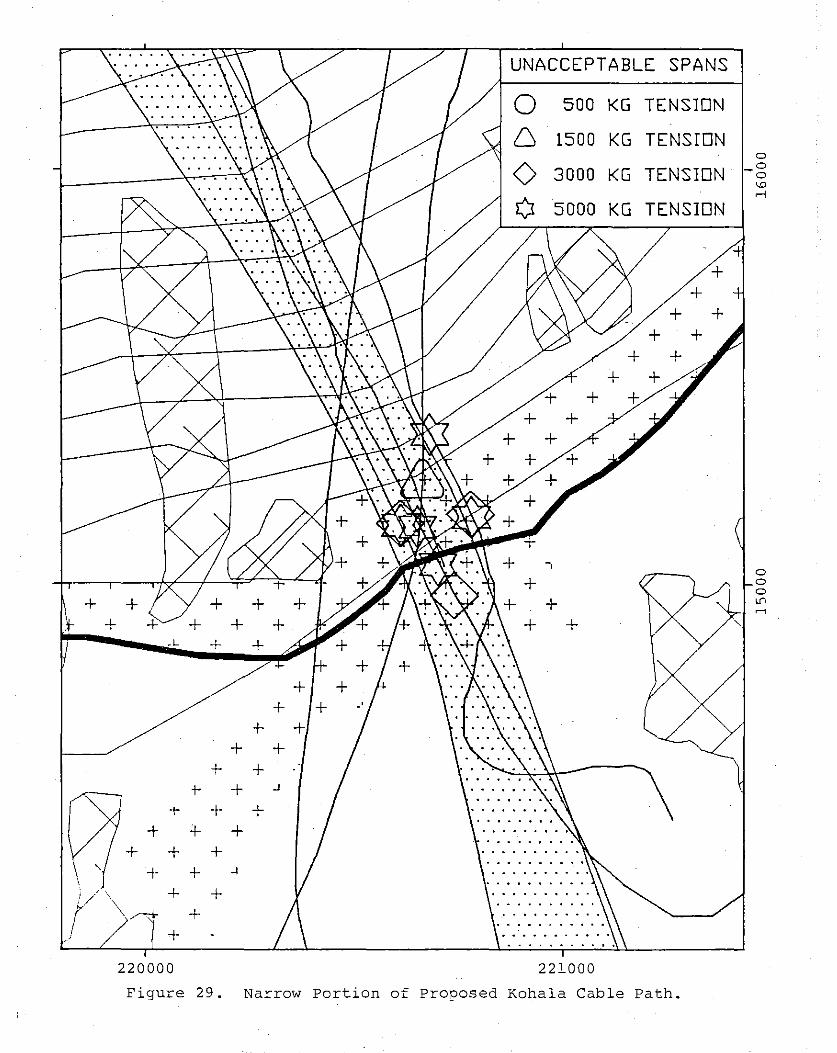
The most critical portion of the selected path on the Kohala side is at the top of the slope. This is illustrated in Figure 29 showing the survey tracks of both the BRS and the Deep Tow that were made in the immediate reg1on. The spans shown are the computed spans along those survey tracks that are in or close to

21

UNACCEPTABLE SPANS

0 500 KG TENSION

6 1500 KG TENSION

0 3000 KG TENSION

0 5000 KG TENSION

21 00 220000 222 00 22

Figure 26. Proposed Cable Path on the Kohala Slope Through Rocky Region & Unacceptable Cable Span Areas.

0 0

0 N

~8.-T2 .,....65.r-T3 /

~ ~

Figure 27. Profile at top of the Kohala Slope, one of the smoother profiles observed during the First Cruise, BRS Track 40. The spans are for 5000 kg (T3) and 3000 kg (T2).

800

900

1000

Figure 28. Negative of Side Scan Mosaic (Fig.2l) Showing Cable Path & Top Edge Kohala Slope.

UNACCEPTABLE SPANS

500 KG TENSlDN

1500 KG TENSION 0

3000 KG TENS JON - 0 0 \.0

'""" KG TENSlDN

-, 0

+ 0 0

+ + + u;

'""" + + + + " .L +

+ + +

+ + + +

+ + t- + -'

-t- + + + + +

+ + + \ ' + + -'

!/ ' \ + + \ +

+ '

220000 221000

Figure 29. Narrow Portion of Proposed Kohala Cable Path.

the selected cable path. Because the bottom in this region is clearly rough, it is difficult to determine the width of an acceptable cable path and the tension at which the cable should be laid in order to assure that there are no unacceptable spans. The following table provides a summary of the unacceptable spans computed from both the first and second channel surveys and shown within the recommended path.

Table 1. Number of Unacceptable Spans Versus Cable Tension

Survey Track 5000 kg 3000 kg 1500 kg 500 kg

BRS Track 40 1 1 0 0 SIO Track 3 0 0 0 0 SIO Track 40 1 1 0 0 SIO Track 51 0 0 0 0 SIO Track 54 1 0 1 0

The number of unacceptable spans in this region clearly is larger for the higher tensions. Track 54, a diagonal track, is the only track showing a span below 3000 kg and this may not be realistic for the cable because of the angle. Note that there is a span at 1500 kg but not at 3000 kg; this is not unusual. In general, higher tensions produce more unacceptable spans but specific locations may have a unique geometry that affects only the shorter spans.

Figure 29 illustrates a recommended path which is 200 m wide but has only been crossed specifically by five survey tracks .which only quantitatively evaluate the path directly below the survey track. The actual roughness between the survey tracks is therefore unknown and therefore there is a finite probability that a cable laid along these unsurveyed areas will not behave as modeled in the above table. There is, however, the basic trend that lower tensions cause fewer spans and this can be seen by looking at all of the analyzed Scripps runs which show a span distribution as follows:

Table 2.

Bottom Tensions

500 kg

1500 kg

3000 kg

5000 kg

Total No. Critical Spans

40

72

82

108

This table suggests that by dropping the tension below 1500 kg, the probability of having an unacceptable span is greatly reduced.

22

Based on this observation and the actual number of spans computed for this region it is recommended that the cable be laid across this region at 1000 kg or less.

The minimum width of the recommended path illustrated in Figure 29 is 200 m and this has been set primarily such that it encompasses the "successful" survey tracks down the slope. The acceptable cable path may well be wider but at this time there are no data to support such a conclusion. If widened, the path could only be enlarged to the east; increasing the western boundary would clearly interfere with some large obstacles further down the Kohala slope. The sidescan gives little support in determining the width of the path as the sidescan shows some roughness which cannot be quantitatively evaluated.

The lower half of the Kohala slope is quite uniform with only a few minor obstructions observed from the sidescan which are avoided as seen in Figure 26. Also, the area above the slope edge is a large, sandy plain that stretches several km inshore. This area is very flat and smooth, with considerable evidence of sand dunes seen in the sidescan.

4.3.3 Photographs, Kohala Slope

Figure 30 illustrates the location of the photographic runs taken along the Kohala slope. Several representative photographs are shown in Figures 31 and 32 with the specific locations of each of the photographs marked in Figure 30. Each photograph was taken at a height of approximately 10 meters above the seafloor and results in a photograph that is approximately 5 m by 7 m. Neither of the photographic runs were along the final recommended path, both being to the west. The Deep Tow system took a total of 457 photographs along these two tracks.

Photograph E in Figure 31 is taken at a depth of 930 m just above the edge of the slope. Most of the photographs taken of this region show a sandy bottom but this particular photograph shows a large, dead coral head.

Photograph F is taken at 980 meters and illustrates the roughest portion photographed along this slope. The rock just below the flash is approximately 2m across. Precision bathymetry from other survey tracks shows this slope rougher than the tracks within the selected path. This is therefore not representative of the selected path. Down slope is to the right in each of these photographs. At the top center of the photograph is a sponge and at the bottom center a sea quill, both attached to the bottom.

Photograph G shows a steep rubble slope at approximately 1170 m depth and is typical of the region from 1050 to 1200 m. These rocks are small, nominally 0.3 m in diameter, and do not represent a major obstacle to the cable.

23

219000

Figure 30.

+ .• + +

+ + + +

220000 221000

Photographed Tracks on the Kohala Slope. Specific Photographs E Through J are in Figures 31 and 32.

0 0 0 co

0 0 0 r--

0 0 0

'"'

0 0 0 L{)

E. Above Kohala Slope, 930 m.

G. On Kohala Slope, 1170 m.

Figure 31.

~ ~~:··

F. Roughest Area, 980 m.

H. Mid Kohala Slope, 1325 m.

Bottom Photographs, Kohala Slope

Photograph H is taken at 1325 m and is typical of the region from 1200 m to 1550 m. This photograph illustrates the basic trend of the size and roughness of the rubble decreasing with depth. The spiral "tree" at the center of the photograph is a gorgonian and the long white line further down the slope is a whip-like coral.

Photograph I, in Figure 32, is a smooth bottom and is seen in both photographic runs between 1425 m and 1640 m. This particular photograph was taken at 1470 m depth.

Photograph J, is the very bottom of the Kohala slope on the western-most track. This photograph shows approximately 1 ft wave ripples on the bottom and is taken at 1930 m.

The photographs presented are typical of both photographic tracks down the Kohala slope with the exception that the western-most track showed fewer large rocks at the top.

4.3.4 Sea MARC Data on the Kohala Side

Once the navigation was corrected for the Kohala side, it was possible to quite accurately match the Sea MARC II data with the Deep Tow sidescan. This was primarily possible because of the very well-defined lava flow structures at the top of the Kohala slope. Figure 20 shows these features quite clearly on the Sea MARC II sidescan image.

The Sea MARC sidescan images show dark regions in some areas that might be interpreted as roughness features but are actually areas with different reflectivity. An example can be seen in Figure 20 with the dark band running just inside the southeast edge of a sandy circular basin at the top of the Kohala Slope. This was crossed several times on b0th the first and the second surveys without noting any features except some extremely small rubble in the Deep Tow sidescan. It appears significant in the Sea MARC data but actually is not for the cable.

4.3.5 First Cruise Data, Kohala Side

The survey data from the two cruises agreed surprisingly well. The primary path recommended during the first cruise was verified on the second; the recommended path remains nearly the same. The Scripps cruise investigated areas further to the east to make a run around that end of the lava flows but in the post-cruise analysis no viable path could be identified.

During the first cruise, the BRS made a single pass 17 km toward Kohala ending at a depth of 270 m. This area was mostly smooth with some high tension spans at 720 m and some more at approximately 500 m. These spans did not result from major features and, being in shallower water and having a wide choice of alternate paths, an acceptable path can most probably be found. No further surveys were made in this region.

24

I. Mid Kohala Slope, 1470 m. J. Bottom Channel, Base Kohala Slope, 1930 m.

Figure 32. Bottom Photographs, Kohala Slope & Below

4.3.6 Final Kohala Cable Path

The final recommended cable path for the Kohala slope is illustrated, without the survey tracks and spans, in Figure 33. The minimum width of this path is 200 m and it will require some maneuvering since the path is not perfectly straight. At the top of the slope, there is significant roughness and it is necessary to lay the cable at 1000 kg tension or less to avoid unacceptable spans. This region is hatched in Figure 33. Like the Maui slope, the recommended tension for the remainder of the path is 3000 kg or less.

Figure 34 is a profile along the recommended cable path on the Kohala side. This profile is generated from actual Scripps Deep Tow bathymetric data.

4. 4 BOTTOM OF THE ALENUIHAHA CHANNEL

4.4.1 General Description and Selected Path

The bottom of the channel with a maximum depth (at the top of the saddle) of 1930 m is generally quite smooth. The region closest to the Kohala slope is predominantly sediment covered with small sediment ripples seen in the bottom photographs and larger sediment waves seen in the sidescan data. Moving toward the Maui side, the channel bottom has a different texture with some scattering of small rocks. Because this portion of the channel crossing did not represent a formidable obstacle for cable laying, relatively few tracks were made completely across the channel. Figure 35 illustrates the tracks and resulting spans from both surveys and the recommended cable path which results from these surveys. Only a single span was observed from a first survey BRS track and the feature causing this span could be identified and the location confirmed with the Scripps sidescan~ The selected path is more than 500 m wide and narrows only along the Kohala and Maui slopes. Bottom tensions do not appear to be a problem. In general it is recommended to be conservative and to lay the cable at as low a tension as is practically achievable by the cable laying control system.

4.4.2 Sea MARC Data

The Sea MARC data validate the conclusions made by both the first and second surveys that the bottom of the channel is relatively smooth. The Sea MARC data are shown in Figure 20. The Sea MARC image also illustrates that there is a difference in bottom reflectivity between the two sides of the channel bottom; there is rubble and small rocks on the Maui side, sand on the Kohala side.

4.5 GEOLOGY (Scripps)

The Deep Tow bathymetric and side-scan sonar data provide much

25

217000

Figure 33.

220000 225000 Final Recommended Cable Path for the Kohala Slope V'ii th Critical •Hdths & Cable Tensions Indicated. Hatched Path Area Requires Low Cable Tension at 1000 Kg.

0 0 0 N N

0 0 0 0 N

0 0 0 L!)

.-<

0 0 0 .-< .-<

HD 'WC CAB E f OUT E: p ROFI LE <KD HAL 1 SI DD

""" ""

iuuL

5ruL

''" """ oon

""' -.... lnrnL . ............

JQfi_

~ l?nn ......___ hnn

--......... '"" --- r---... I'"' ;:;;;;--..,

bon ...... r---

leon .....___

1900 . r--

""""

Figure 34. Profile Along the Recommended Kohala Cable Path.

UNACCEPTABLE SPANS

0 500

u 1500

0 3000

0 5000

KG TENSION

KG TENSION

KG TENSION

KG TENSION

216000 218000 Figure 35. Bottom of Alenuihaha Channel Showing Both

Deep Tow & BRS Survey Tracks, Spans & Rocky Areas Observed with Side Scan.

0 0 0

"' "'

0 0 0 0

"'

·.·.·.·.·.·.·.·.·.:.;-. 0 • 0 0 0 0 0 • 0 \0

0 0 0 0 • • • 0 •

0 • 0 0 0 ,o • 0 0 •••

0 0 0 0 0 •• 0 0 0

216000 218000

Figure 36. Recommended Cable Path across the Channel Bottom

0 0 0 N N

0 0 0 0 N

more topographic detail than the previous Sea MARC survey, but little additional geologic insight.

On the Maui slope the lobate benches are strewn with lava rubble, and are probably the surfaces of major debris flows that originated by subaerial erosion of the island. However, we cannot exclude the possibility that they represent old lava flow surfaces; even if they are, the data suggest that they are the submarine extensions of flows from subaerial vents, rather than the product of local submarine eruptions. The steep fronts of the benches, though covered by either lava or debris flows, may have originated as tangential fault scarps, i.e., the head-walls of major slumps caused by gravitational stresses.

On the steep slope of the Kohala side the close-spaced downslope "gullies" seen on the Sea MARC images were found to have very slight relief. Bottom photographs show that they are low ridges of rubble with intervening strips of sandy sediment. Most probably the sand strips fill inactive debris chutes once used for downslope transport of material (including coral litter) from the Kohala Terrace. At the very steep crest of this slope we photographed large unjointed boulders, light gray in color, that could well be weathered coral. No typical pillow lava, diagnostic of submarine lava flows (especially flows from submarine vents) were photographed on the slope, but patches of sheet-flow lava presumed to have originated by post-erosional eruptions along Kohala's principal rift zone were observed on the terrace surface.

At all depths on both sides of the channel abundant current ripples were photographed on the patches of sandy sediment. Ripples include both symmetric types indicative of oscillatory flow (probably related to internal waves), and high-energy asymmetric ripples indicative of relatively fast (i.e., more than 0.5 knot) bottom currents, dominantly in a southwest direction. The surface of the sedimentary fill in the floor of the channel has larger scale sand waves, about 10 m in average wavelength. These are especially well developed near the foot of the Kohala slope.

26

5.0 CONCLUSIONS AND RECOMME~IDATIONS

5.1 ROUTE LOCATION AND CABLE LAYING

1. A continuous path, but not an easy one, has been found that may be adequate for a commercial cable across the Alenuihaha channel.

2. The path width, required bottom cable laying tensions and the bottom roughness have been defined for this selected cable route.

3. Precision cable laying will be required on both the Maui and the Kohala sides of the channel, but more so on the Maui side for accuracy, more so on the Kohala side for tension.

4. The bathymetry along a survey track has an accuracy of 10 m and the multiple surveys agree within 5 m.

5. . Key obstacles are located to a 10 m accuracy, possibly better.

6. The positioning and bathymetry is adequate for laying the test cable except for possibly tying in the key obstacles into the cable laying navigation grid just prior to the cable lay.

7. No further surveys of this type are required for the HDWC Program.

B. The bottom of the recommended cable path is primarily smooth, spans are not a problem and low cable laying tension is not required except at the top of the Kohala slope where a low tension of 1000 kg is recommended. All other locations along the path have a recommended cable tension of 3000 kg or less.

9. As concluded in the first cruise, it is better to lay the cable at a low tension rather than a high one to avoid unacceptable spans.

10. Figure 37 summarizes the location and width of the final recommended cable route.

27

21 000 2 000 220000 Figure 37. Cable Path across Alenuihaha Channel

0 0 0 0 M

0 0 0 l1)

"'

0 0 0 0

"'

0 0 0 l1)

.....

5.2 SURVEY OPERATIONS (Scripps Institution of Oceanography)

1. Ability to track the towed vehicle and control its path relative to previous passes was an essential element in successful exploration of the complex terrain. An effective, real time, near bottom acoustic navigation capability was a major element; however, the existence of continuous tracking of the towing ship using the Mini-Ranger provided the effective means for controlling our maneuvers, as well as supporting reconnaissance passes outside the area covered by the acoustic system.

2. The most important lesson was that one should not try to cut costs by using a ship that is marginal for the job. In this we were fortunate, (although it did not seem so initially) that R/V NEW HORIZON's bow thruster was damaged and that R/V MELVILLE was available. We were doubly fortunate that Scripps Institution of Oceanography was both willing and able to cover the substantial increased costs, to carry out the operation.

3. R/V MELVILLE provided two elements which were superior to R/V NEiv HORIZON by so much that it meant the difference between a highly satisfying operation and one which would have been continuously on the edge of success. First was R/V MELVILLE's very effective maneuverability, due to the availability of powerful side thrust at both ends of the ship. In spite of consistent 20 to 30 knot winds, we were able to put our tracks where we wanted them. R/V NEW HORIZON would have been much more difficult to control.

4. The other element was the availability of enough living and working space to be able to mount a significant data processing effort in parallel with the primary data collection effort. This meant that, particularly in the latter part of the operation, we could choose our tracks in optimum fashion in relation to data already acquired. If anything, we could have used one or two more people in the data processing department.

5. Having Van Ryzin and Noda on board, complete with their own computers and knowledge of the cable laying requirements, to interact with our group on a real time basis was an important plus. Once we had learned each others' capabilities and operating methods this worked well. Particularly on the Maui side the close cooperation which developed between the ship operators, the MPL data processors and the HD&C contractors led to a solution which would not have emerged otherwise.

28

6. It seems clear that sea floor survey and positioning technology, as exemplified in our Deep Tow system, is capable of meeting requirements appropriate .to the cable route selection and evaluation problem in the context presented. Our profile accuracy, in spite of our best efforts, did not consistently achieve 15 em depth resolution - there was often a surface wave induced component not completely canceled by the vehicle's pressure (depth) sensor. On steep slopes there were also occasional instances in which the uphill specular reflection would override weak return from below the vehicle in spite of our sidelobe levels being 18 db down. On the other hand, the topography itself was such that the few good segments were not obscured by this effect, and the bad segments were very obvious. In addition, because of good ship control and navigation, we were able to re-run critical segments to verify their profiles.

7. The Deep Tow system and its computer complex operated reliably and effectively. Of the total of 213 hours we were away from the pier, 7% were spent in transit, 5% on transponder launch and recovery, 84% actually towing and the remaining 4% was for equipment checkout, repair and personnel transfer. We covered a 17 km wide band on the Maui side and 7 km on the Kohala slope, locating satisfactory paths on both sides, although there were only narrow gaps at some points.

B. The existence of prior data (basic topography, SeaMARC II and Ocean Bottom Roughness Recorder) was useful in indicating regions in which we should concentrate our efforts. Some correlations between the SeaMARC II long range SLS data and Deep Tow near-bottom SLS records were made. However, the continuity of the band of rough terrain in the 1200 to 1500 m depth zone on the Maui side was not obvious from those records. It would have been particularly useful to have had a swath sounding topographic map of the area having the depth precision and spatial resolution of a Sea Beam survey, done in the Mini-Ranger coordinate system. Not only would this have facilitated operation of the Deep Tow vehicle and choices of tracks, it would have let us choose better locations for transponder launches, particularly in relation to the sharp topographic break on the south side.

9. With regard to future operations of this type our recommendations would be for more of the same: select survey equipment and operators having extensive, successful deep ocean experience, use a ship that can clearly do the job, and assemble a seagoing team that can provide insights into all aspects of the problem.

29

10. With regard to this site we feel that the area covered (including the Mini-Ranger navigated portions outside the acoustic transponder net) has been adequately explored. There might be additional options outside that zone. If significant extra costs are indicated from analyses of the cable laying requirements for the paths identified during this survey, then it could be useful to expand the area. Short of that, the next step would seem to be an actual, on-site, laying of a dummy cable through the most d iff icul t portions of the path. This might be preceded by a run with a submersible or high quality ROV along the entire track to verify that no small but disturbing factors exist at some localized place.

5.3 DATA PROCESSING

1. The at-sea operations and data processing worked well together and the necessary near real time decisions required for directing the survey and homing in on an adequate path were possible.

2. There is excellent agreement in all forms of data between parallel tracks, cross tracks, first and second cruise, and Sea MARC data.

3. The span analysis on the detailed bathymetric data was hindered somewhat due to noise in the data but this could be overcome by careful manual interpretation and parallel data.

4. The bottom cable span analysis continues to be a valuable tool in path evaluation since it is the only quantitative method available.

5. 4 MAUI SLOPE

1. The Maui slope region above the saddle area in the Alenuihaha Channel is a complex series of terraced escarpments through which it was difficult to wind a continuous path.

2. As a result of the excellent agreement between sidescan, precision bathymetry and Sea MARC, the surveyed portion of the Maui slope is now known well and an overall map of this region has been prepared.

3. Major obstacles on the Maui slope occurred at the 1000 m level, 1200 m level and 1500 m level.

4. The bottom of the recommended path is smooth in all regions and cables can be laid at a tension up to 5000 kg without unacceptable spans. 3000 kg or lower tensions are recommended, if possible.

30

5. The path width is 400 m and wider in most locations with the exception of a narrow portion at 90V m depth which is 170 wide and the narrowest portion at 1200 m depth which is 80 m wide.

6. The recommended Maui path is not straight with the sharpest bend occurring at 1000 m depth at a 500 m to 700 m turning radius.

7. The shallowest portion of the recommended path is 550 m; the survey did not extend inshore of this point.

B. Much of the survey time was spent searching for alternate cable paths and extending the search far to the east and the west of the originally planned area. Orienting the Sea MARC data relative to the Deep Tow tracks during the post-cruise analysis indicated that there are potential routes both further to the east and the west of the actual search area and one possible route short-cutting the sharp bend radius at 1000 m in the proposed cable path. Neither of these potential routes can be confirmed on the basis of the present data.

9. For the search area covered, it is unlikely that there is an alternate acceptable path in the 1200 m to 1500 m region.

5.5 KOHALA SLOPE

1. The Kohala side of the channel is more easily defined with one single steep slope from 930 m to 1930 m and with several lava flows at the top of the slope.

2. The lava flows at the top of the slope and the considerable roughness at the top edge of the slope are the major restrictions to a cable path.

3. The lower portions of the Kohala slope were predominantly smooth.

4. A path cannot be found across the top of slope that is free of unacceptable spans for a cable laid at 3000 kg or greater.

5. The only means found of crossing the upper portion of the Kohala slope without an unacceptable cable span is to lay the cable at a low tension of 1000 kg or less.

6. The acceptable width of the Kohala path at the top of the slope is difficult to determine by sidescan since it is only a qualitative tool and the area has some roughness. The final selected width of 200 m encompasses the region traversed by 5 separate survey tracks.

31

7. Alternate paths along the Kohala slope were considered but not found to be acceptable. An attempt was made at a path far to the east but that proved unacceptable. This survey did not prove, however, that an acceptable path does not exist in this region.

5.6 CHANNEL BOTTOM

1. The bottom of the channel is predominantly smooth, sediment covered on the Kohala side and with some small scale rubble on the Maui side.

2. A wide, fairly straight path has been found across the channel bottom.

5.7 RECOMME1IDATIONS

1. Although the majority of the cable path has a smooth bottom and no unacceptable spans are expected for cable tensions up to 5000 kg, lower tensions of 3000 kg or less are recommended, if operationally feasible, in order to further minimize the probability of unacceptable spans.

2. An additional survey with a submersible or ROV in the narrow regions on both sides of the channel would help in further understanding the cable path for the HDWC program. This would particularly be valuable at the top of the Kohala slope and at the 1200 m narrow region on the Maui slope.

3. For precise cable laying, it will be necessary to tie in the position of the major constraining obstacles into the cable laying navigation grid prior to laying the cable.

4. Because of the extreme topographic variations, particularly on the Kohala slope, great care will be necessary in the placement of the bottom transponders in any future acoustic navigation grid.

5. Before laying the commercial cable, further surveys of the route should be made concentrating along the selected path & insuring that all areas are 100% covered by sidescan and all questionable targets investigated with a BRS/Deep Tow fine resolution bathymetry system.

32

REFERENCES

1. Campbell, J. Frisbee, "Hawaii Deep Water Cable Program Phase II At-Sea Route Surveys", University of Hawaii at Manoa--Hawaii Institute of Geophysics, December, 1983.

2. "Characterization of Potential Routes and Route Option Selection", Ralph M. Parsons Co. DBA Parsons Hawaii, May, 1985.

3. "Hawaii Deep water Cable (HDWC) Program Revised Cable Catenary Study", Pirelli Cable Corporation, October, 1985.

4. Love, A.E., A Treatise on the Mathematical Theory of Elasticity, Fourth Edition, Dover Publications, New York, 19844.

5. Hawaii Deep Water Cable Program Bottom Roughness Survey of the Alenuihaha Channel", Makai Ocean Engineering, Inc., Ed Noda & Associates and Hawaii Institute of Geophysics, May, 1986.

6. Spiess, F.N., "Alenuihaha Channel Deep Tow Survey", Scripps Institution of Oceanography University of California, San Diego, November, 1986.

7. "Hawaii Deep Water Cable Program (HDWCPJ Conceptual Design of Reduced Scale At-Sea Test Draft Report" Hawaiian Dredging & Construction and Makai Ocean Engineering, December, 1986.

8. Spiess, F.N., Lonsdale, P.F., "Deep Tow Rise Crest Exploration Techniques", Marine Technology Society Journal, Vol 16, No. 3, 1982.

33

APPENDIX A

Reference: HAWAII DEEP WATER CABLE PROGRAM BOTTOM ROUGHNESS SURVEY OF THE

ALENUIHAHA CHANNEL

Prepared by: Makai Ocean Engineering, Inc.

Ed Noda & Associates Hawaii Institute of Geophysics

May 1, 1986

SUMMARY" OF THE FIRST BOTTOM ROUGHNESS CRUISE

An eight-day Bottom Roughness Cruise was performed in October/November, 1985, of the Alenuihaha Channel using the 110ANA WAVE and a bottom roughness survey package specifically developed for this cruise. This survey was the first detailed look at the bottom roughness in the Alenuihaha Channel. Its purpose was to characterize the bottom roughness in terms meaningful to the HDWC cable laying process. It attempted to find an acceptable cable path across the Alenuihaha Channel, identify the degree of placement accuracy required for the successful deployment of the cable, to identify an optimal bottom cable tension and to identify the needs for subsequent surveys. In addition to accurately measuring the bottom roughness, the first survey included operating the Sea MARC II, a wide-swath sidescan sonar system, over the area.

The overall survey system is illustrated in Figure 2. The Bottom Roughness Sampler (BRS) was towed at 20 to 30 m off the bottom along a desired survey track. The sampler measured and recorded the BRS depth, Z, and the height above the bottom, H. The sum of these two measurements provided an accurate recording of the depth of a 1.5 m diameter sample area directly below the BRS. The BRS contained a pressure transducer which measured Z to a 15 em resolution and a 500 kHz echo sounder which measured H to a 2 em resolution. A data logger on the BRS recorded the z, and H at 1 second intervals. Also on the BRS was a 12 kHz pinger which provided a direct and bottom reflected signal to the surface ship for controlling the BRS altitude above the bottom.

Figure 3 illustrates the primary areas surveyed during the first cruise. Area A is a steep North Kohala slope and was believed to be representative of the roughest terrain to be encountered by the HDWC cable. The steep slopes on the Maui side were also surveyed, Area B. Areas Cl, C2, and C3 were also surveyed but with less emphasis. Prior Sea MARC cruises and bottom sampling cruises had shown the bottom of the Alenuihaha Channel is primarily sediment.

Figure 4 illustrates Sea 11ARC data that was collected prior to the October cruise. This side scan record clearly shows the steep Kohala slope, possible lava flows above the Kohala slope and a variety of irregularities along the Maui slope. The bottom of the Alenuihaha Channel is relatively clear.

Typical bottom data collected by the Bottom Roughness Sampler are illustrated in Figures 5 through 7. The BRS proved to be a

valuable tool in that it did provide bottom roughness resolution within 15 ern; data from which cable spans and bend radii could be predicted.

One disappointment for the first cruise was that the bottom long-based acoustic positioning system did not function and therefore the absolute position of the observed bottom obstacles are not accurately known. The BRS position has been estimated by knowing accurately the ship's position, ship's speed, BRS depth and the cable length out. The positions of the bottom features are probably known within 150 rn.

Figure 8 illustrates the location of all the successful data tracks during the bottom roughness survey. Extensive coverage was done in both areas A, B and in C. This survey was extended to get at least one track all the way from Hawaii to Maui, at least within the range of the electronic positioning system.

Observations: Kohala Slope, Area A

Figure 9 illustrates the location of significant features observed from the track profiles. Most of the roughness on the Kohala Slope occurs between 950 rn and 1100 m. The area between 1100 m to 1920 m is smooth for almost every track and with a relative roughness which is uniform and less than 0.5 rn. In contrast, every track in the 1000 rn range showed significant bottom roughness with outcroppings from 3 to 10 rn. Because of the difficulty at the top of the Kohala Slope, 3 tracks were made along the upper edge, parallel to the contours (Tracks 17 and 22) • These cross tracks clearly illustrate several lava flows on the eastern side of the upper Area A. These lava flows can also be seen in the Sea MARC data illustrated previously. Tracks 15 and 39 also traverse these lava flows illustrating features up to 15 rn high.

Track 23 was run parallel to the contours at about the 1400 rn contour. This track graphically illustrates (Figure 10) that the Kohala Slope has a series of ridges and valleys that run perpendicular to the contours and that it is not a perfectly uniform slope.

The final run made in Area A was Track 40, illustrated in Figure 11, which is on the western side. This was an attempt to cross the apparently clear areas shown by the Sea MARC data and to avoid the lava flows which were observed to the east. A 20 rn escarpment was discovered above the 900 m mark; this is probably the edge of the basin-like structure observed in the Sea MARC data directly above and slightly to the east of Area A. Track 40 also shows significant bottom features at the top of the Kohala Slope and some unusual roughness between 1600 and 1700 m. The very bottom of Track 40 shows some roughness of 2-3 m elevation.

ALENUIHAHA BOTTOM ROUGHNESS SURVEY HAWAII DEEP WATER PROGRAM

::0 0

"' Ol -

RIY MOANA WAVE

400 M TYP.

.75 M/S

BOTTOM ROUGHNESS SAMPLER (BRS)

7'

POSITIONING TRANSPONDER

FIGURE 2

SHIP POSITIONING & GUIDANCE BRS POSITION DATA LOGGING BRS ALTITUDE (WINCH) CON1ROL

II II II II II II II I I I I I I

I I I I I I I I I I I

POSITIONING 1RANSPONDER

DATA LOGGER: 1/SEC

12 KHZ PINGER

3000 lb LEAD

500 KHZ ECHO SOUNDER, 4' TOTAL BEAM, 2cm RESOLUTION. MEASURE H

PRESSURE 1RANSDUCER, 15 em RESOLUTION MEASURE Z

l-,_ 1.5 M DIA --.J..--M~AX SAMPLE AREA

The cruise has also further isolated areas of concern which will required more survey work during the second survey. Most notably these areas are at the top of the Kohala slope at the 1000 m contour and between 1000 m and 1600 m along the Maui slope. In addition to finding areas of concern, large areas have been identified that are relatively smooth and do not represent a major challenge to cable laying, from the standpoint of bottom roughness. These areas include the lower portion of the Kohala slope, the bottom of the channel, and the shallow water near Kohala.

The first cruise has not identified a continuous path across the Alenuihaha Channel nor has it identified the width of the path in any of the areas where the roughness was acceptable. Furthermore, the position of the tracks and the obstacles identified along the tracks are only known to an accuracy of approximately 150 m, unsuitable for the identification of an actual cable route. ·

and another level of significant roughness at 1500 m. All these regions are separated by smooth areas. Several cross runs were made, Tracks 28, 29 and 30 in the region of most significant roughness between 1000 m and 1400 m depth. These tracks showed that the eastern portion of Area B is quite smooth. Prompted by this data, Track 45 was run on the western slope only to find very large escarpments at 1200 m and at 1500 m. The Sea MARC data showed a potential path in the regions of Tracks 41, 42 and 43. These tracks, however, show significant roughness (10 to 15 ml and escarpments in the region between 1000 and 1300 m.

Figures 14 through 18 illustrate Track 21 with resultant cable spans a various tensions. Only the critical spans are shown, which are a function of cable tension, for example, the critical span length, at 3000 Kg tension, is 37.7 meters or greater. At all tensions, there are unacceptable spans and quite probably unacceptable bend radii.

As for the Kohala Slope, no obvious path was found on the Maui side. The most difficult region for finding an acceptable path will probably be in the region between 1000 m and 1600 m in depth. Above and below this range, there is considerably more clear space and a higher probability that an acceptable path can be found.

Observations: Shallow Kohala Slope, Area C3

An extended series of tows were made, (Tracks 35 through 38) in the shallow region of the Alenuihaha Channel on the Hawaii side (Figure 19) • In other shallow regions on the island of Hawaii old coral reef structures create significant underwater obstacles. For this particular series of tracks, the vast majority of the bottom was fairly smooth. Some regions of rock outcrops occur between 700 and BOO m depth and between 300 and 400 m. Most of these obstacles are felt to be isolated ones and can probably be avoided by taking parallel tracks.

Conclusions

The primary accomplishment of the preliminary cruise has been that the general level and distribution of roughness along the cable route in the Alenuihaha Channel has been identified. Many major roughness concerns prior to the cruise have been eliminated such as the existence of continuous and impassable escarpments or a bottom that is extremely rough everywhere.

The first cruise has greatly increased confidence that an acceptable cable route can be found. Precision cable laying will probably be required during the commercial program but, if required, it will be isolated to specific locations and be a small percentage of the overall cable laying.

Track 40 was evaluated by analytically laying a cable along the profile at 3000 Kg bottom tension, and subsequently yielded no critical spans. There are however, several spans which are nearly critical in length. These spans are close enough to the critical value to be considered as undesirable in that they may easily become critical due to the realistic complexities of a true laid cable shape. At 5000 kg tension, there are clearly critical spans but at 500 kg tension, no critical spans. The critical spans for the 5000 kg.tension (two) are shown in Figure 12, an enlarged portion of Track 40. There were no critical spans in any other area of Track 40.

A clear, wide and obviously smooth path has not been found through the Kohala Slope region. The primary areas of difficulty will be between 850 m and 1100 m depth. For the deeper regions, there appear to be many acceptable cable paths. In the region between 950 and 1000 m there is a great deal of difference in roughness between parallel paths, there is no general trend that shows one track as better than another. In the shallower regions above the steep slope, however, there is a large lava flow to the east and this will probably narrow the search for a final cable path to the general region of Track 40.

Observations: Channel Bottom

The channel bottom, region C2, is fairly smooth and does not have any major features but it is not only smooth sediment as previously anticipated. The ends of Tracks 21 and 40 both show · rocky areas with 2-3 m elevation, sufficiently uniform and without enough elevation to cause unacceptable spans and bend radii. All the tracks on the Maui side at the 1800 m depth range show relatively uniform ripples, perhaps sand waves, of approximately 4 m elevation from trough to peak; these are not significant to the cable.

Observations: Maui Slope

The Maui slope was the most complex area to try to piece together during the cruise. There are large features distributed over the entire slope and it was difficult to determine any particular pattern. Figure 13 illustrates the bottom features seen in the Maui tracks. Very large escarpments ranging from 20 m to 150 m were observed at a variety of locations but they did not align themselves along any particular contour.

The first Maui tracks that were run, number 21 and number 31 illustrate that the slope is relatively smooth above 1000 m and that there are large, smooth areas interdispersed with areas of significant roughness and escarpments. At 1000 m depth, both Tracks 31 and 21 illustrate a large escarpment, perhaps the front of a lava flow, that is 60 to 100 m high. These two tracks also show a smaller escarpment between 15 and 40 m high at 1300 m depth

A

20 25'

FIGURE 3: Specific survey sites in the Alenuihaha

Channel: Cruise #1

Figure 4 Sea Marc data from Alenuihaha Channel. A and 13.

previous Boxed areas

surveys in the are survey sites

~

11r ·11 Ttf 4V~ II ~ ~~ 711'1 rr 1 rn wnmrrrl 11 lT' ·1 11 nn

1 -ECHO ' GUNDER

bnn

TR, CK 3 Rnn KO ALA SL PE

ktnn

F;nn

I I c_nn

I ~ , \ bnn

v 1-BRS LOWER NG

Rnn

h / f-P RESS U E

i=lnn

lf [11 nflllllln '"'\ [ v BOTTOM

II Ill 111 1111)

nnn

11 nn ' \.1~

II-I~ ~ l?nn I I I I I I I I I I _, 10 MIN I- ~ l':lnn

FIGURE 5: Typical BRS data showing the pressure, altitude, and bottom data.

·1w 1

I

[\

TRACK 4 1850 M

PRESSURE

1900 M

BOTTOM

10 MINUTES

1950 M FIGURE 6: Track 4 at the base of the Kohala Slope illustrating the BRS movement

due to vessel heave and the relatively smooth bottom, Spikes in the

bottom are caused by unreturned echos in the profiler.

TRACK 11 OUTCROP AT 1050M KOHALA SLOPE

PRESSURE (BRS)

1 METER INCREMENTS

FIGURE 7: Outcrop on Kohala Slope at 1100 m. Note individual data points.

The horizontal scale equals the vertical scale.

KILOMETERS 0 5 10

FIGURE 8.

ALENUIHAHA CHANNEL BOTTOM ROUGHNESS

SURVEY PLJI.NNED

HAWAII DEEP WATER CABLE PROGRAM

SURVEY TRACKS

DEPTHS IN METERS

SPAN SYMBOLS 0 - T1 (500 Kg)

0 - T2 {3000 Kg)

¢ - T3 (5000 Kg)

FIGURE 9

~.

<D c ..., CD

23

T E3

-;::;

- t - E::.'

.:::

~.

C':l c: -s ro ,_. ,~

Inn RACKI40 Pnn

hon ! i

~00 I Is on '

' l ~ .. 1

I

17oo i :

~00 ! I

i I ' ' hnnn I

i I ' ' 1100 '

~?00 i i I

""" '

'"" I i

L500 •

~ ' i '

17M ' ·~

I ' 1 LBOO I i iooo i I : """" I

I ' l '--' I i i

I ' ' ! i

I ' I • ' i i

' i ! ' I I

' I I ' i . I ! j !

; i i i I ; I

1 I _j '

! ' I I

: I I i i

i ' i i ' ' ' •

I I i i I I I l -;----... ' ! I

-· i I

l l ! I I

i I i i ' I

I I ' I I i

I I i : I : I

' : I i I i I i ! ! ' ' TRAC 40 - VIEIJ A I i ! i I i ! ! -

i . i : -... t-., : i I

I i SPANS vs TENSION Kh I

_-..._ I i I

~~ t ~~~g--f2 ' l ! : ..... t-,

i ! l~QQ ,; I i ..... I ' --...,. I '

' I I ......___ I I

' ' I ---+--- ' ' I ! i !

I : ' ' I i I : . I

! I I L

_l _l

-n ~.

"' c. ... C1)

...... N

TRAC < 40 -

/38.-T2 /"65.

/

VIEW A .

t-T3

~ ~ ~

.............

------

'oo

<oo ......_ ___ .Joo

1oo sao

SPAN SYMBOLS 0 - T1 (500 Kg)

<) - T2 (3000 Kg)

0 T3 (5000 Kg)

Figure 13

• [,., TRAC ~I

~- 1 ...

1 ... r~

r~

r--lm RACK l- v EU A

[,., -.. r- T AC -[,_ " fs VS ENSlDN <ET 1 ACK 2 VI \1 C

lu" -30 ,, [,., -11300 r, ... r u...

T ACK 2 - Vl v E

r.- L" [,_ r ....

21 1 ....

. .., ~.

<0 c .., f1)

..... ""'

. 21A

- rRACK /

(

c::; c::; - r: ~42.-T2

~

)1 v ~EW A

r---_________ ------1----.. -

. --

I

TRACK 21 IEW -

3 --

- - . 5t .-T3

-------- /'

" . /49.-p 41.-T ------ .

' --r---

I

2lB

~-

<C c .., CD

21C

---- - .. ---- ------

I T r

i h I ! I

' i i I I

! i i !

'

' i

' ' I i .____ _________ ,_ ---

----------------- -----

) A c K 2 "-

--------- --------·--------

-------------------- -

v I 1- w c I -- 1- :

- 1-:

' I I I

I I ! i I

I

! 65. T3 ' I 49. T2 .

I ! ;

I • I

I I

i

---- -------------- .. ------- ----·· .- ---------- ------ -------· -----·---- ---- _j

~---·-· ----------- ----+-·--·-·-------------- ··-·-------!---· .. ·--·--·---------··---- ·----··-:-~ TRACK 21 -1_ __ \LI E 'vJ D •

.., ~-

lO c: --'--­..., co ' 44.-T2

25.-Tl 51.-T3

~------+----==:====~~~~--_1--T

21D

I i I

L_ ---·-·- --·-·

i ' i I

.. -·------· --···--·---·- --+ ___ j

··'

7oo

600

----400---1-

-Jo . 0

Figure 19

APPENDIX B

PLAN FOR THE SECOND

BOTTOM ROUGHNESS SURVEY CRUISE

OF THE ALENUIHAHA CHANNEL

JUNE, 1986

HAWAII DEEP WATER CABLE PROGRAM

FINAL - REVISION 3

May 15, 1986

INTRODUCTION

This document is a general plan for the second Bottom Roughness Cruise of the Alenuihaha Channel for the Hawaii Deep Water Cable Program. The survey will be conducted by the Scripps Institute of Oceanography utilizing the vessel NEW HORIZON and the research vehicle DEEP TOW in June of 1986. This plan outlines the goals, requirements, schedule and surveying techniques: it is to be used as a guideline in preparation for this cruise.

The Hawaii Deep Water Cable Program is responsible for determining the technical feasibility of laying multiple underwater power cables between the islands of Hawaii and Oahu in the Hawaiian Islands. Figure 1 shows the proposed cable route between the islands. One major obstacle identified early in this program was the Alenuihaha Channel, 1920 m deep between Maui and Hawaii and shown as the survey area in figure 1. The Alenuihaha Channel had been selected for a more detailed feasibility study because of its extreme depth, very steep slopes and relatively recent geology.

The Hawaii Deep Water Cable is a large structure with a wet weight of 27.1 kg/m and a diameter of 11.8 em. This cable is laid on the bottom at a nominal tension (5000 to 500 kg) in order to prevent kinking during the laying process: if laid on a rough bottom the cable will be bent over obstacles or suspended between obstacles in free spans. The severity of these bends and the length of the spans is a function of the botto~ roughness. The cable could be damaged during the laying process if the bend radius is less than 1.5 m, a value established by Pirelli Cable Corporation for this cable. Another failure mode is fatigue caused by either vortex or tidal induced oscillations over time in a free span subjected to cross currents. An analysis by Pirelli has determined an acceptable free span length: this acceptable span length is a function of the bottom cable tension. As an example, a free span greater than 38 m in length at 3000 kg tension is unacceptable.

It is necessary to lay the cable on the bottom in the Alenuihaha Channel without unacceptable spans and without unacceptable bend radii. The size of the cable spans and the severity of a cable bend is a function of the bottom roughness. In order to determine the difficulty and the cost of laying the cable, the bottom roughness must be determined.

An eight-day Bottom Roughness Cruise was performed in October/November, 1985, of the Alenuihaha Channel using the MOANA WAVE and a bottom roughness survey package specifically developed for this cruise. This survey was the first detailed look at the bottom roughness in the Alenuihaha Channel. Its purpose was to characterize the bottom roughness in terms meaningful to the HDWC cable laying process. It attempted to find an acceptable cable path across the Alenuihaha Channel, identify the degree of placement accuracy required for the successful deployment of the

Page 2

cable, to identify an optimal bottom cable tension and to identify the needs for subsequent surveys. In addition to accurately measuring the bottom roughness, the first survey included operating the Sea MARC II, a wide-swath sidescan sonar system, over the area. A cruise report is available with all the profiles and side scan data illustrated.

Figure 2 illustrates the primary areas surveyed during the first cruise. Area A is the steep North Kohala slope and was believed to be representative of the roughest terrain to be encountered by the HDWC cable. The steep slopes on the Maui side were also surveyed, Area B. Areas between the primary targets were also surveyed but with less emphasis.

The primary accomplishment of the preliminary cruise has been that the general level and distribution of roughness along the cable route in the Alenuihaha Channel has been identified. Many major roughness concerns prior to the cruise have been eliminated such as the existence of continuous and impassable escarpments or a bottom that is extremely rough everywhere.

The first cruise has greatly increased confidence that an acceptable cable route can be found. Precision cable laying will probably be required during the commercfal program but, if required, it will be isolated to specific locations and be a small percentage of the overall cable laying.

The first survey cruise has also further isolated areas of concern which will require more survey work during the second survey. Most notably these areas are at the top of the Kohala slope at the 1000 m contour and between 1000 m and 1600 m along the Maui slope. In addition to finding areas of concern, large areas have been identified that are relatively smooth and do not represent a major challenge to cable laying, from the standpoint of bottom roughness. These areas include the lower portion of the Kohala slope, the bottom of the channel, and the shallow water near Kohala.

The first cruise has not identified a continuous path across the Alenuihaha Channel nor has it identified the width of the path in any of the areas where the roughness was acceptable. Furthermore, the position of the tracks and the obstacles identified along the tracks are only known to an accuracy of approximately 150 m, unsuitable for the identification of an actual cable route.

Page 3

SURVEY AREA

Figure 3 is a section of NOAA Chart #19320 showing the Alenuihaha Channel and the shoreline at Maui and North Kohala. In previous cruises shore stations have been established on Maui for electronic navigation. Figure 4 is a general profile of the Alenuihaha Channel along the approximate cable route. The first bottom roughness cruise showed that the upper edge of the steep Kohala slope (1000 m depth on the Hawaii side) is quite rough but the lower portion of the slope and the bottom of the channel is smooth in most areas. The slope irregularities seen on the Maui side are the result of a rather bumpy slope. Parallel tracks down the Maui slope can sometimes appear quite different.

Figure 5 is a detailed bathymetric chart of the Alenuihaha Channel. Bathymetry is based on NOAA data with the contour lines generated by the Hawaii Institute of Geophysics at the University of Hawaii. Two primary survey areas, A and B, are marked on this chart and represent the area where a wide acceptable cable path will be most difficult to find and where some precise commercial cable laying will probably be necessary. Based on the results of the first cruise, Figure 6 illustrates the most likely paths for the cable.

Page 4

SURVEY GOALS & REQUIREMENTS

The following are the goals for the second Alenuihaha Bottom Roughness Survey:

1. Find the "best" path possible, for one cable, through the areas of the Alenuihaha Channel crossing that have been determined by the first cruise to be the most difficult.

These areas are illustrated in Figure 6, The "best" cable path is the path with no unacceptable spans or bend radii and requiring the least difficulty for cable laying that can be found within the survey time and equipment constraints, Evaluating the "best" path discussed in a following section.

2. Collect sufficient data on the worst portion of the best cable route such that the cable laying control requirements can be defined.

This information will form the basis of the cable laying control criteria and set the requirements for the At-Sea Test. This most difficult portion of the cable route is anticipated to be a relatively small portion of the entire route and probably less than 1 km in length. It is a requirement of this survey to evaluate and select this site during the survey in order that more thorough information can be collected at that location before the end of the cruise.

3. Find parallel routes for an additional two cables.

Measurements Required

Roughness

It will be necessary to measure the bottom roughness directly under the towed vehicle. The roughness measure desired is similar to that obtained by the Bottom Roughness Sampler during the first cruise, A vertical accuracy of 0,1% and a vertical resolution of 15 em is necessary for a sample area 1.5 m in diameter, The sampling rate should be such that the horizontal spacing of data points should be 1 m or less. Horizontal resolution (along the path) should be 1 m.

In order to evaluate at sea the suitability of a particular path, the profile must be immediately plotted with the horizontal and vertical scales equal and at approximately 1:2000 scale. The ability to replot the data at 1:500 scale of isolated areas of roughness is important.

Page 5

Vehicle Positioning

The vehicle positioning must be tied into the Hawaii State Grid, Zone 2, (Maui)--a transverse Mercator projection. The first cruise used this projection with units in meters. The bottom accuracy with a long-based acoustic positioning system should be 6 m or better with a resolution of 1 m. The first cruise used shore-based electronic positioning systems on Maui, and these will be used during the cable laying tests and the actual cable deployment; to achieve the accuracy required and to maintain continuity between various at-sea efforts, a similar system must be used.

Side Looking Sonar

In order to eva·luate the path width, a sidescan system detecting obstacles out to 100 m on either side of the vehicle is necessary at the normal operating elevation of the vehicle off the bottom during bottom roughness sampling. The side scan record should be available in real time, or nearly real time, and readable for immediate interpretation such that a potential path can be quickly evaluated. The configuration should be such that the ability to detect significant cable obstacles is maximized.

A wider span side scan capability for initial searches is necessary with a search pattern at 200 m or greater t0 either side of the vehicle. This system would be invaluable as an intermediate step between the Sea MARC data which will be available prior to the cruise and the fine resolution, close-bottom surveys which are done along potential cable routes. This can be accomplished by flying the vehicle at a higher elevation.

Photography

Photography along the selected route is necessary. In particular, photographic coverage of the major obstacles at the worst portion of the best route are needed and enough photography to geologically characterize the bottom is desirable.

Video

It is anticipated that intermittent video coverage of the bottom in real time may augment the search process and assist in giving the operators a visual picture of the bottom roughness measured. This is desirable, but not mandatory.

Page 6

RESPONSIBILITIES

The following are the general responsibilities of the participants during the second survey cruise

HAWAIIAN DREDGING AND CONSTRUCTION:

Hawaiian Dredging has overall responsibility for the performance of the cruise including ensuring the availability of required labor, materials and equipment and the technical accuracy of all work.

SCRIPPS:

Scripps has total responsibility for providing and operating all the required surveying equipment, particularly the Deep Tow system and the New Horizon such that the program goals can be accomplished, The sole equipment exception is the Mini Ranger positioning system as noted under Edward K. Noda's responsibilities, Dr Fred Spiess will be Chief Scientist during the cruise.

MAKAI OCEAN ENGINEERING, INC:

Makai will provide Dr Joe Van Ryzin, Sr Ocean Engineer, to represent the HDWC program and to evaluate the bottom data obtained in order to select a particular cable path. He will work with the Scripps data, computers, and plotters in order to evaluate the bottom data in terms meaningful to cable laying and to plan areas suitable for further surveying.

EDWARD K. NODA AND ASSOCIATES

Noda and Associates will provide a Mini Ranger surface navigation system for the cruise. They will set up, maintain, and take down the shore stations during the cruise. In Hilo, with the assistance of the Scripps crew, the shipboard receiver will be installed and connected to the Scripps' computer, Dr Ed Noda will be on board during the cruise to assist Makai in the data interpretation and be responsible for the continued operation of the navigation system.

Page 7

DATA DELIVERED

Hawaiian Dredging through its subcontractors will provide the following data prior to the cruise:

1. A complete data package and report on the first cruise. 2. The Sea MARC II data from the previous and preceding

cr.uises. 3. Charts showing the specific sites to be surveyed and the

most likely routes.

Scripps' data collection and deliverables are the following:

Scripps, During Cruise:

1. Side Looking Sonar (SLS) real time plots plus Polaroid copies of areas of interest for comparison and interpretation during the cruise.

2. Sounder profiles - real time analog plots of the high precision bathymetry vs time.

3. Sounder profiles - real time (nearly) of digitized profiles vs time, digital sum of pressure and down signal.

4. Accurate navigation plots of the ship and Deep Tow, occasionally corrected for looping and navigator errors.

5. Accurate time correlation between all records 6. Plots of accurate profiles of selected tracks as depth vs

distance (not time) on a large scale. 7. Fortran span analysis on selected tracks (operated by Makai

and Noda on the Scripps' computer). B. Photographs of selected areas, Black and white negatives

developed from one camera during cruise. 9. Sub-bottom profiler plots.

Scripps, Immediately after cruise:

1. Clean navigation plots of the whole cruise 2. Navigation plots with observation notes, Polaroids, etc. 3. Photographs of SLS plots of best paths 4. Representative photographs (negatives, one roll from each

lowering) 5. .Plotted profiles done during the cruise 6. Depth vs distance data files including navigation

positioning that have been processed during the cruise (presumably transferred on board to a PC computer for storage on diskettes).

7. Loan to HD&C the SLS records and other important "raw" data while the Deep Tow group is conducting the.following cruise (and cannot be working on the report)

Scripps, 2 to 4 wks after cruise:

1. Corrected navigation data after checking the looping and, in particular, along the selected cable route locations. Provide on 9-track tape.

Page B

Scripps, Final Report (Sept 30}:

1. Corrected Navigation chart in the Hawaii State Grid system. 2. SLS mosaic in cable path areas. 3. Detailed profiles of each track, in depth vs distance. 4. Digital data on 9-track of combined (navigation and

bathymetry} and corrected x,y,z, and time data. 5. Ge<Jlogical interpretation of the areas surveyed. 6. Microfilm of SLS analog records. 7. Photographs- 35 rom slides. B. Plots of bathymetry contours of search area, 5 m spacing,

with and without paths, concentrating along cable path areas and within capability of survey data

9. Sub bottom profile data summary. 10. Cruise narrative 11, Summary, recommendations, and conclusions.

Makai Ocean Engineering will take the bathymetry and navigation data from scripps and interpret the bottom roughness and selected paths relative to the HDWC cable laying process. Makai will provide a preliminary and final report from this data:

Makai, immediately after the cruise:

1. Presentation of the cruise preliminary results including selected paths surveyed, photographs, and representative data.

2. Identification and characterization of the worst portion of the best path surveyed for purposes of the cable control study.

Makai, final report:

1. Profile plots along selected paths showing cable spans and unacceptable cable bend radii.

2. Description and location of the final cable path(s) selected - including roughness, slope, width, and curvature.

3, Recommendations.

Page 9

SCHEDULE

Cruise: June 2 June 16 June 17-25 June 26-27+

Data Processing July B July, mid

July, mid Sept 30

Cruise Schedule:

New Horizon leaves Scripps Pick up JVR, EN at Hila, depart for channel Survey Arrive Snug harbor B am, off load.

and Reports: Initial reduced data, navigation and photographs Preliminary Cruise report and presentation to DOE/Parsons Define control problems Final Reports, Scripps and Makai

The following provides a general guideline for the cruise and an allocation of time relative to the importance of each task and the difficulty anticipated. Total time is nearly 9 days, 210 hours. Priority is established (A) through (C) - (A) being the highest priority.

1. Transit - (A)

Travel from Hila to Alenuihaha and Alenuihaha to Honolulu: 14 hr s total.

2. Transponder deployment and recovery - (A)

Deploy and, after the survey, recover the transponders for the bottom navigation system. Deploy the transponders such that both the Kohala slope and the Maui slopes are all covered and that the survey can jump back and forth across the channel, allowing time for data processing and interpretation in a given area before selecting more surveying paths. Ten hours of survey time is anticipated.

3. Initial Sidescan Survey- (A)

The initial sidescan survey will further refine and orient the Sea MARC II data, correcting positions of major obstacles and providing finer resolution. The most likely cable paths identified as a result of the previous survey and the Sea MARC data can be accurately located relative to the long base navigation system. A single tow along the top of the Kohala slope can identify and locate unique bottom features. At least two tows up and down the Maui slope will be required since that

Page 10

slope is more complex. It is expected that this will take approximately 10 hrs of the total surveying time.

4. Path Location - (A)

Run a series of surveying tracks collecting bottom roughness data and fine resolution sidescan along a variety of possible cable routes. Evaluate each route and select a "best" path. The path width during this survey will be defined by the sidescan and will be somewhat qualitative as to whether the roughness observed is too severe for the cable lay; where necessary, multiple parallel tracks may be necessary, collecting more bottom roughness data to better def~ne the path width. It is anticipated that Area A (Kohala) will require 36 hrs of the surveying time and Area B (Maui) will require 60 hrs. '

5. Detailed Survey of the Worst Area - (A)

On the basis of the previous step, the path with the lowest value rating will be identified. This area would be the most challenging relative to cable laying requirements and needs to be detailed further. Multiple parallel passes collecting bottom roughness data will be required in this area. If this more detailed survey shows that the area is far more objectionable than previously anticipated, an alternate path may have to be found. Forty hours of the total surveying time is tentatively allocated for this task.

6. Connecting Tracks - (B)

Areas A and B have been identified in the first survey as the most formidable challenge to cross with the cable. If time allows, detailed paths should be surveyed between the best paths found in Areas A and B and continuing the path south toward Kohala. Much of the connecting paths can be obtained while traversing between the two areas. Sixteen hours of the survey time is allocated for this task.

7. Additional Cable Paths - (C)

The above steps concentrate on a single cable path. Depending upon the width of that path, it may be suitable for all three or only one cable. Parallel cable paths should be located for the other two HDWC cables. In particular, parallel paths should be found adjacent to the worst area as detailed in Step 3. Twenty-six hours of the survey time can be allowed for this task.

Page 11

ACCEPTABLE PATH DEFINITION

The primary goal of the second survey cruise is to find a best acceptable route for the cable across the Alenuihaha Channel. It will therefore be necessary to evaluate the route in terms that are meaningful to the cable laying process and to make decisions at sea toward selecting the "best" route. This was not a requirement of the first survey cruise which only had to define the bottom roughness. It is the purpose of this section to define what constitutes an acceptable path and which paths are more acceptable than others.

Roughness Considerations

As discussed in the introduction, bottom roughness can cause an unacceptably short bend radius of the cable or excessively long free span lengths which cause cable fatigue. These two modes of failure are not necessarily independent; a small bend radius is usually associated with a long span but could exist alone. It will be necessary during the cruise to evaluate the bottom roughness both in terms of potential bend radius and potential span lengths.

The minimum bend radius has been defined by Pirelli to be 1.5 m for the commercial cable. Computing a bend radius of a cable with a particular stiffness and weight laying on an irregular bottom is quite difficult and time consuming. For this cruise a series of simplified criteria will be established by which the bottom roughness can quickly be evaluated for excessive bend radius. For example, a 4 m high isolated rock on a flat bottom will yield a 1.5 m bend radius; a lower rock is fine, a higher rock is not. A criteria somewhat more complicated than this will be established relating adjacent rocks and general slope of the bottom.

Excessive free span length is the other failure mode for the cable on the bottom. Pirelli has established the following maximum free span cable lengths as a function of bottom cable tension:

Bottom Tension

5000 kg 3000 kg

500 kg

48.2 m 37.7 m 19.6 m

Maximum Span

The higher bottom tensions are easier to lay and result in much longer allowable spans but, as has been seen in the evaluation of the first cruise data, there are fewer unacceptable spans if the cable is laid at a low tension as opposed to a high tension. Therefore, as the bottom becomes more irregular there will be the need to lay the cable at a lower tension in order to not produce unacceptable spans. A computer method will be used to quickly evaluate a given area of bottom roughness for potential unacceptable spans and to evaluate the tension at which the cable would have to be laid in order to not have any unacceptable spans.

Page 12

It is anticipated that during the cruise the bottom roughness profile will be plotted and areas of roughness can be checked to determine if an unacceptable bend radius would occur and at what tension, if any, the cable would have to be laid in order to avoid any unacceptable span lengths. If either the bend radius or the span lengths are unacceptable, the path is unacceptable.

Path Width Considerations

Because of the great depth and cotisiderable currents in the Alenuihaha Channel, it is difficult to precisely lay the cable on any given path and the degree of difficulty is obviously a function of the width of the available path. As the path becomes narrower, different techniques may be required in cable laying. While a definition of these techniques is still underway, the following is provided to the approaches anticipated in accurately positioning the cable on the bottom.

1. Path Width Equals 25% of Depth

If the path width is greater than or equal to 25% of the depth, there will be no difficulty in positioning the cable within this path. Only rough observations of the currents would have to be made and few, if any, corrections made in the surface track of the ship,

2. Path Width Equals 10% of Depth

As the path decreases to 10% of the bottom depth, more precise laying will be required involving a computer evaluation of the cable shape, ship position and instrumentation of cable tensions, vessel positions and speed and current profiles.

3. Path Width Equal 5% of Depth

As the path width decreases further, transponders will be required to be placed on the cable and interrogated by a bottom transponder grid as a means of periodically checking the cable laying accuracy. The computer-aided control can then correct for actual measured deflections of the cable behind the laying vessel.

4. Twelve Meter Bottom Laying Accuracy

As cable precision is decreased to a 12 m path width, immediate and almost continuous feedback will be required from the touchdown point on the bottom. An extensive transponder grid on the bottom is anticipated with a relatively high density of transponders attached to the cable during the laying process.

5, Two Meter Bottom Laying Accuracy

For an extremely narrow cable path, a pre-laid guide rope would be deployed (possibly on a trial and error basis),

Page 13

surveyed and checked prior to laying the actual cable. The electrical cable would be laid on top of the guide rope utilizing video feedback from an ROV following at the touchdown point. This procedure has been used by Pirelli Cable Corporation in the past for laying a cable through rough terrain across the Straits of Messina but not at depths approaching those in the Alenuihaha Channel.

It·is obvious that the wider paths will be more desirable than the narrowest path. On the basis of the first survey data, it is felt highly unlikely that a cable path equaling 25% of the depth will be found over the whole distance and that certainly the capability will be required on the cable laying barge to lay the cable along a path as narrow as 10% of the depth. On the other hand, it is certainly hoped that the 2 m and possibly even the 12 m path widths can be avoided. There is no indication in the data from the first cruise that these may be necessary.

The spacing between the cables is primarily determined by a repair criteria. In less than 500 m of water, the repair method would most likely be by grappling the cable, splicing in a new section and laying the bight on the bottom. There must be room on one side or the other for this bight to be placed on the bottom, the bight would require approximately 500 m clearance. If two cables are laid on the bottom, they could be laid side-by-side and, in the case of repair, the bight would be laid on the outside of the pair. If three cables are laid on the bottom, two could be laid side-by-side but the third would need to be laid at least 500 m to one ~ide of the pair.

When considering laying cables below 500 m depth, the cables would not be grappled nor any bights laid on the bottom. The repair method would be by picking up the cable at the shallow end until the damaged section is reached, splicing in a new cable and then relaying the cable until a depth is reached at which the bight could be laid. In this case, the cables could be laid in close proximity to each other but should not cross, each one should be clear for lifting.

When considering laying two or more cables along a given path in either shallow or deep water, the difficulty of laying has to be taken into account. For example, if a 600 m wide path is found on the bottom and evaluated for its potential for laying all three cables, the effective cable route is only 200 m for each cable and that amount of cable laying precision will be required.

Path Straightness

It is very unlikely that any given path across the Alenuihaha Channel will be a perfectly straight line and the cable will need to be maneuvered from one desirable heading to another. Sharp turns in the cable path, however, are not acceptable because the cable is laid under tension on the bottom. As the bend is made the bottom cable will have a tendency to slide and possibly bend over a bottom obstacle. As a general guideline, the path plan

Page 14

radius should not be less than 1000 m and any angular deviation should be kept less than 15 degrees.

Under very precise bottom laying conditions, as with laying with the guidance of acoustics or with an ROV on the bottom, a very low bottom tension would most likely be used and the path maneuverability could be quite high. It is difficult at this time to place a lower limit on the maneuverability radius; it should be kept as lar~e as possible.

Path Value Factor

When all the above considerations apply to a cable path, there results a rather complex definition of what is acceptable and what is not. Laying the cable with a high tension along a very wide path which lS perfectly straight is obviously the most desirable situation but it is also highly unlikely to be found. The surveyor will invariably be in the situation of comparing two potential paths, neither of which is perfect.

On the following page is an illustration of applying a value factor to potential cable paths with different characteristics. This table is not complete but is included here for the purpose of being an indicator of the evaluation approach that is intended for this cruise. Prior to the second survey cruise, this table will be further evaluated to the point that it is a usable tool during the cruise. The intent is to place a value on any given survey path and the goal of the surveyor will be to select the path with the highest value factor.

It is obviously more difficult to lay the cable along narrow path and to lay the cable at a very low but positive bottom tension. It is also difficulty to maneuver the cable around obstacles on the bottom. The table on the following page is intended to tell the surveyor, for instance, that it may be more desirable to select a narrower path with a high cable tension than for a very wide path which requires a very low cable tension.

0 500

1000 1500 2000 2500

HAWAII

............. 1'--... -..... I'-

..... f-""

FIGURE 4: Profile of Survey Area, Alenuihaha Channel Scale is 1 to 1. Units in Meters

MAUl

KILOMETERS 0 5 10

Figure 5

ALENUIHAHA CHANNEL BOTTOM ROUGHNESS

SURVEY

HAWAII DEEP WATER CABLE PROGRAM

POTENTIAL ROUTES

DEPTHS IN METERS

Page 15

TABLE 1 PATH VALUE FACTORS This table gives the relative value of potential cable paths, all

without unacceptable cable spans or bend radii. The path is characterized by its width, required cable tension, and path straightness and is valued by considering the technical difficulty and risks of deploying the cable along that path.

(Path width modifications and path value factors will be added later.)

MIN WIDTH.m TENS.kg

Conventional laying accuracy 25% depth 5000 25% depth 5000 25% depth 3000 25% depth 3000 25% depth 1000 25% depth 1000

Precision laying, 10% depth 10% depth 10% depth 10% depth 10% depth 10% depth

computer aided, 5000 5000 3000 3000 1000 1000

STRAIGHT

straight r=l000/150 straight r=l000/150 straight r=l000/150

current monitoring straight r=l000/150 straight r=l000/150 straight r=l000/150

VALUE

100

occasional use of 5% depth

transponders 5000

to calibrate laying straight r=l000/150 straight ~;=1000/150 straight r=l000/150

accuracy

5% depth 5000 5% depth 3000 5% depth 3000 5% depth 1000 5% depth 1000

Acoustic precision avoidance limited obstacles 12 meter 5000 straight 12 meter 5000 r=l000/150 12 meter 3000 straight 12 meter 3000 r=lOOO/lSo 12 meter 1000 straight 12 meter 1000 r=l000/150 12 meter <500 straight 12 meter <SOO r=l000/150

Following pre-laid guide rope, video feedback from ROV 2 meter 5000 straight 2 meter 5000 r=l000/50 2 meter 5000 r<lOOO,>SO 0 2 meter 3000 straight 2 meter 3000 r=l000/50 2 meter 3000 r<lOOO,>SO 0 2 meter 1000 straight 2 meter 1000 r=lOOO/SO 2 meter 1000 r<lOOO, >5° 0 2 meter <500 straight 4 2 meter <500 r>lOO 3

--

ROUTE OPTION 2

e I II t• ..... c w 4 •••••

N

0

SURVEY AREA

·--·-FIGURE 1: Proposed HDWC Cable route and area of

deep water roughness study

KILOMETERS 0 5 10

ALENUIHAHA CHANNEL BOTTOM ROUGHNESS

SURVEY

HAWAII DEEP WATER CABLE PROGRAM

SURVEY TRACKS

DEPTHS IN METERS

Figure 2: Tracks Surveyed, Cruise #1

,.

"

;, '

c

...

... ... +

I

I 48$ _,'463

8, ... -· ::::r o\77..1:/

509

g; ~{

4s;..

Figure 3

\,, \ 498

I \'23 \

\J3 \: .. \ \ . \~52 474

436

••

,.. '" .. ,

...

•,

gy

409

' 3:

0

\

gyS

. '' ... ~ ............. ' .... / I<AUIHI /EAl> f65 24- i~i 189 ••• 43 "0 351 'I ' 22 ,,

/ 544 ' !fSO) 331 /!147

I /

,. 66~

.,, ... '' ... 529 57>

'" 660 vus I

"' "' .·hi ••• ,.,

,,s / ••• ' '

790

708 / ... • •• tOO

I eap ' ...

/ ,.,... .... ···

/ ' .,. _, _ .. .. i03~

' .. // / 965' / ....

... - / IIJO

/ 1075

1060 ' .'

I ' 1420

1079 / 1370

""' i2~J)1

145~

'7~

1056 '' 1107 ""·-""/"- ....... __

1300

830 ..... I ~.

i~O$ !t50 E L ....... 1247 --:' - . - .A. N 1{ ... --, .. ... c H:- "' . · ........

I 493

471 /11-!""'1 ...

449

439 406

..o 381

322

IF I; 391 ~- " ..... JIEI.::•

' 307 i

I 295

310

J79

.. , •• I

357

""' "'" 247')'

.'

"'

...

383 ... ':.(-8;\/ ....,,,,"1 ,f\'.·1.'.

?fl'(h.:t.f"i.' II'.

280

of' ~....,; 230

... 186 171

15.1 C. S SJt

113 121

"' .. -

I I.ah.iki~,.

:

KILOMETERS 0 5

Figure 5

ALENUIHAHA CHANNEL BOTTOM ROUGHNESS

SURVEY

HAWAII DEEP WATER CABLE PROGRAM

POTENTIAL ROUTES

DEPTHS IN METERS

---~

APPENDIX C SCIENTIFIC PARTY AND SHIP'S CREW

SCIENTIFIC PARTY

Marine Physical Laboratory

F. N. Spiess, Chief Scientist

D. Boegeman, Principal Engineer

C. Lowenstein, Computer Engineer

R. Lawhead, Programmer

R. Elder, Engineer

T. Clary, Electronic Technician

G. Austin, Marine Mechanician

M. Linzer, Data Processing

A. Foster, Data Processing

C. Paull, Asst. Scientist

M. Mcintyre, Res. Asst.

B. Lougee, Res. Asst.

Others

F. McHale, HDC

J. Van Ryzin, Makai Ocean. Engr.

E. Noda, Ed Noda Assoc.

P. Walsh, HECO Consultant

G. Pillard, SIO Res. Tech.

D. Stuber, SIO Comp. Tech.

C. Clark, Volunteer Asst.

SHIPS FORCE

c. Johnson, Master

D. McGuire, 1st Off.

D. Murline, 2nd Off.

M. Stein, 3rd Off.

L. Hulsrna, Seaman

G. Achenbach, Seaman

R. Jackson, Seaman

s. Lewis, Seaman

A. Santos, Bos'n.

c. Jones, Cook

A. Velasques, Cook

R. Fish, Chief Engr.

p. Bueren, 1st Asst. Engr.

M. Breen, 2nd Asst. Engr.

D. Herman, 3rd Asst. Engr.

M. Hotchkiss, Oiler

s. Martin, Oiler

w. Bradley, Oiler

J. Being, Electrician

P. Polk, Radioman

s. Jackson, E. T.

M. Aspeytia, Wiper

APPENDIX D SHORE NAVIGATION STATION LOCATIONS

Two navigation shore stations were located on Maui at the following locations:

Location

Kahikinui

Muolea

X

190789.6 m

219737.0 m

y

31274.0 m

39543.7 m

z

439 m

98 m

These x and y locations are relative to the primary navigation grid used for both this survey and the previous survey. The grid is the u.s. Coast and Geodetic Survey Transverse Mercator for Hawaii State, Zone II, Maui. All units of measurement are in meters.

The above shore stations were used for both surveys and are easil1 and accurately reproducible for further work. Their exact locations have not been surveyed precisely, the absolute position of the shore stations is within 10 meters.

The Kahikinui benchmark is located on a rectangular co~cl~l~ water tank shown in Figure 1. Figure 2 provides a sketch of the water tank area which is located about 240 ft from the Piilani Highway. The benchmark is a 3/4" galvanized pipe which has been bolted to the outer makai face of the concrete tank, and is about 2 ft above the tank top. The water tank is owned by Annette and Kimo Niles, P.O. Box 234, Kula, Maui, 96790, Ph: (ll 878-6816.

The other benchmark station is located at the home of Mrs. Ernest C. Gray. Figure 3 shows the location of Mrs. Gray's home in Muolea, Maui. Figure 4 shows the specific description of the property owned by Mrs. Gray where the house is parcel l with an area of 2.23 acres. Figure 5. is a partial sketch of the lot, where the benchmark is a pipe imbedded in a rock wall makai of the second story lanai. Mrs. Gray is now living in Kaneohe and the property is being managed by her son, Charles Gray, Gray Associates, 820 Mililani Street, Suite 610, Honolulu, Hawaii 96813, Ph: 524-4220.

2o·~;·6L.,cc,.c-------,--------..;ro;;oo.rn------;--------;-..,;f,;,----,.,---------;--------,.-------'-,-;-----,,'<,.---,-•

Figure 1: Kahikinui Water Tank Location. Topographic Data from USGS 7-l/2 Minute ~lap, Lualailua Hills, Hawaii, County of Maui

I

11

1,..----- ~R""E'\.- Rci>,D

I I

~~~L.t::

?1/o/ 4/<1.)) PI"" ~W\eD \D Q O~ee'fei \JJA"'f«L -------..._______ "It< >I"'- ov..-reoz. 1.01<1.-'- +-~+--="

~It( lA~ Z.:

i-<:it>i:l \<(1 r-.lu..1 B"'~CJ!.•-<1.~ Ulc.A1'-ow

412<J""O f'"L<>oe. --t­~1Z<><M'

2 '-' """"'~ LAI.>Ao'I.

1='itl.the..e 0: Me£. e".c.. c,e.A·(;. :-\ot.!<? 3e""L."''-'"'e..~

\..0 U.\tDo..j

,;;~o>e.u.e

v.e..;.. s;.c.. G.•'-><-<s ~

' r"· '"-v u~y ,..~~• .. <kulo• PI

".}<l Pl

HAWAII-MAUl CO. ISLAND OF MAUI-HANA DISTRICT

7,5 MINUTE SERIES (TOPOGRAPHIC) 1~E(5)

MAS. E.C. GRAY'S HOME AND BENCHMARK LOCATION

1)0000

FEET

+ •o·

Figure 3: Mrs. Ernest C. Gray's Home Location. Topographic Data from USGS 7-1/2 Minute Map, Kipahulu, Hawaii, County of Maui

/

DEPARTMENT OF THE TAX COMMISSIONER

TAXATION MAPS BUREAU HRRITORY Of HAWAII

TAX MAP SECOND DIVISION

ZONE I SEC. I PLAT

I 5 07 CONTAINING PARCELS

SCALE: 1 IN. : 200 FT

. . ··~ ...

3 , __ --..L

Figure 4: Mrs. Ernest C. Gray's Property, Plot No. 3 =

. -· ~.

i..D

7

c.

9

8

c

Millon

/. 5'.