hawawini & vialletchapter 121 valuing and acquiring a business

Hawawini & Viallet Chapter 12 1

Chapter 12

VALUING AND ACQUIRING A

BUSINESS


Background Objective of chapter

How to value a business• Either that of its assets or of its equity

The focus is on the methods most commonly used in valuing firms: Valuation by comparables Valuation by discounting the cash flows from the firm’s

assets Valuation using the adjusted present value approach

OS Distributors is used to illustrate the methods Firm was also analyzed in Chapters 3-5


Background After reading this chapter, students should

understand: The alternative methods used to value businesses

and how to apply them in practice to estimate the value of a company

Why some companies acquire other firms How to value a potential acquisition Why a high proportion of acquisitions usually fail to

deliver value to the shareholders of the acquiring firm Leveraged buyout (LBO) deals and how they

are put together


Alternative Valuation Methods Most common approaches to valuing a

business: Valuation by comparables

• Comparing a business to similar firms in its sector, Discounted cash flow or DCF valuation

• Based on discounting a business’ future cash-flow stream at a required rate of return

Other measures of a business’ value: Liquidation value Replacement value


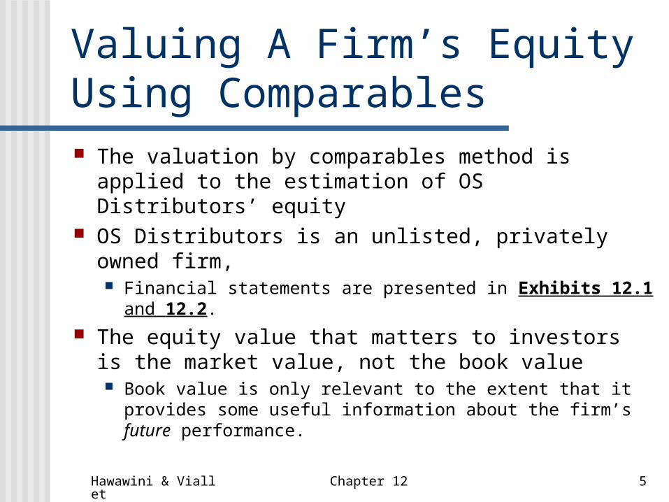
Valuing A Firm’s Equity Using Comparables The valuation by comparables method is applied to the

estimation of OS Distributors’ equity OS Distributors is an unlisted, privately owned firm,

Financial statements are presented in Exhibits 12.1 and 12.2.

The equity value that matters to investors is the market value, not the book value Book value is only relevant to the extent that it provides some

useful information about the firm’s future performance.


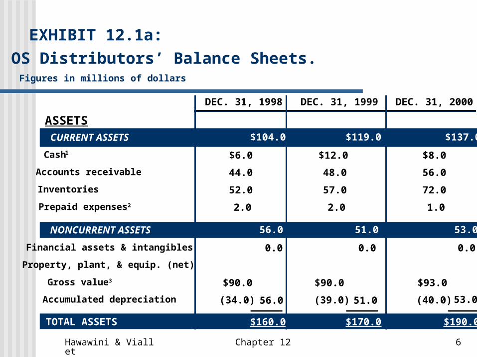
EXHIBIT 12.1a:

OS Distributors’ Balance Sheets.Figures in millions of dollars

DEC. 31, 1998 DEC. 31, 1999 DEC. 31, 2000

ASSETSCURRENT ASSETS $104.0 $119.0 $137.0

Cash1 $6.0 $12.0 $8.0

Accounts receivable 44.0 48.0 56.0

Inventories 52.0 57.0 72.0

Prepaid expenses2 2.0 2.0 1.0

NONCURRENT ASSETS 56.0 51.0 53.0

Financial assets & intangibles 0.0 0.0 0.0

Property, plant, & equip. (net)

56.0 51.0 53.0

Gross value3 $90.0 $90.0 $93.0

Accumulated depreciation (34.0) (39.0) (40.0)

TOTAL ASSETS $160.0 $170.0 $190.0


EXHIBIT 12.1b: OS Distributors’ Balance Sheets.Figures in millions of dollars

LIABILITIES AND OWNER’S EQUITYCURRENT LIABILITIES $54.0 $66.0 $75.0

Short-term debt $15.0 $22.0 $23.0

Owed to banks $7.0 $14.0 $15.0

Current portion of long-term debt

8.0 8.0 8.0

Accounts payable 37.0 40.0 48.0

Accrued expenses4 2.0 4.0 4.0

NONCURRENT LIABILITIES 42.0 34.0 38.0

Long-term debt5- 42.0 34.0 38.0

Owners’ equity6 64.0 70.0 77.0

TOTAL LIABILITIES ANDOWNERS’ EQUITY $160.0 $170.0 $190.0

DEC. 31, 1998 DEC. 31, 1999 DEC. 31, 2000


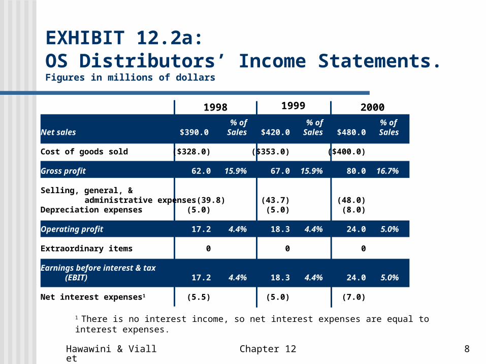
EXHIBIT 12.2a: OS Distributors’ Income Statements.Figures in millions of dollars

1998 1999 2000

1 There is no interest income, so net interest expenses are equal to interest expenses.

% of % of % of Net sales $390.0 Sales $420.0 Sales $480.0 Sales

Cost of goods sold ($328.0) ($353.0) ($400.0)

Gross profit 62.0 15.9% 67.0 15.9% 80.0 16.7%

Selling, general, & administrative expenses (39.8) (43.7) (48.0)

Depreciation expenses (5.0) (5.0) (8.0)

Operating profit 17.2 4.4% 18.3 4.4% 24.0 5.0%

Extraordinary items 0 0 0

Earnings before interest & tax(EBIT) 17.2 4.4% 18.3 4.4% 24.0 5.0%

Net interest expenses1 (5.5) (5.0) (7.0)


EXHIBIT 12.2b: OS Distributors’ Income Statements.Figures in millions of dollars

1998 1999 2000

Earnings before tax (EBT) 11.7 3.0% 13.3 3.2% 17.0 3.5%

Income tax expense (4.7) (5.3) (6.8)

Earnings after tax (EAT) $7.0 1.8% $8.0 1.9% $10.2 2.1%

Dividends $2.0 $2.0 $3.2

Retained Earnings $5.0 $6.0 $7.0


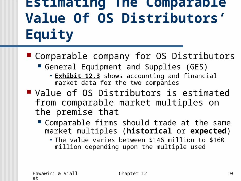
Estimating The Comparable Value Of OS Distributors’ Equity

Comparable company for OS Distributors General Equipment and Supplies (GES)

• Exhibit 12.3 shows accounting and financial market data for the two companies

Value of OS Distributors is estimated from comparable market multiples on the premise that Comparable firms should trade at the same market

multiples (historical or expected)• The value varies between $146 million to $160 million

depending upon the multiple used


EXHIBIT 12.3a: Accounting and Financial Market Data for OS Distributors and GES, a Comparable Firm.

GES OS DISTRIBUTORS

Accounting data (2000)

1. Earnings after tax (EAT) $63.5 million $10.2 million

2. “Cash earnings” = EAT $63.5 + $57.5 = $10.2 + $8 =+ depreciation expenses $121 million $18.2 million

3. Book value of equity $526 million $77 million

4. Number of shares outstanding 50 million shares 10 million shares

5. Earnings per share or EPS [(1)/(4)] $1.27 $1.02

6. “Cash earnings” per share [(2)/(4)] $2.42 $1.82

7. Book value per share [(3)/(4)] $10.52 $7.70


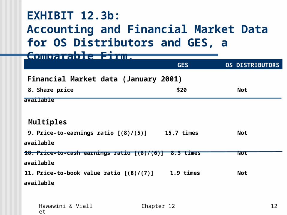
EXHIBIT 12.3b: Accounting and Financial Market Data for OS Distributors and GES, a Comparable Firm.

GES OS DISTRIBUTORS

Financial Market data (January 2001)

8. Share price $20 Not

available

Multiples

9. Price-to-earnings ratio [(8)/(5)] 15.7 times Not

available

10. Price-to-cash earnings ratio [(8)/(6)] 8.3 times Not

available

11. Price-to-book value ratio [(8)/(7)] 1.9 times Not

available


Factors That Determine Earnings And Cash-flow Multiples

Earnings and cash earnings multiples are affected by General market environment

• Such as the prevailing level of interest rates Factors unique to companies

• Such as their expected growth and perceived risk

DCF formula is used to explain why• Companies with high expected rates of growth and low

perceived risk usually have high multiples• Multiples increase in an environment of declining interest

rates


Factors That Determine Earnings And Cash-flow Multiples

When comparing values of firms in different countries (and even in different industries within the same country) Cash earnings multiples should be used

rather than accounting earnings multiples• Neutralizes some of the distortions introduced by

differences in accounting rules across countries (and across industries within a country)


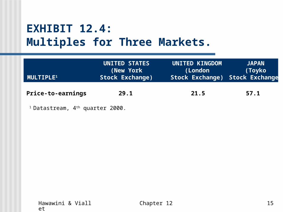
EXHIBIT 12.4: Multiples for Three Markets.

UNITED STATES UNITED KINGDOM JAPAN(New York (London (Toyko

MULTIPLE1 Stock Exchange) Stock Exchange) Stock Exchange)

Price-to-earnings 29.1 21.5 57.1

1 Datastream, 4th quarter 2000.


Valuing A Firm’s Assets And Equity Using The Discounted Cash Flow Approach

Estimating the DCF value of a firm’s assets According to the DCF method, the value of an asset

is determined by • Capacity of that asset to generate future cash flows

Starting with the case of a company with no expected growth, we

• Examine the impact of factors such as expected growth and risk

• Provide general formulas to value assets, cash flows and cost of capital


The impact of the growth of cash flows on their DCF value The faster the growth rate in cash flows, the

higher is their discounted value The impact of the risk associated with

cash flows on their DCF value The higher the risk of a cash-flow stream, the

lower is its discounted value



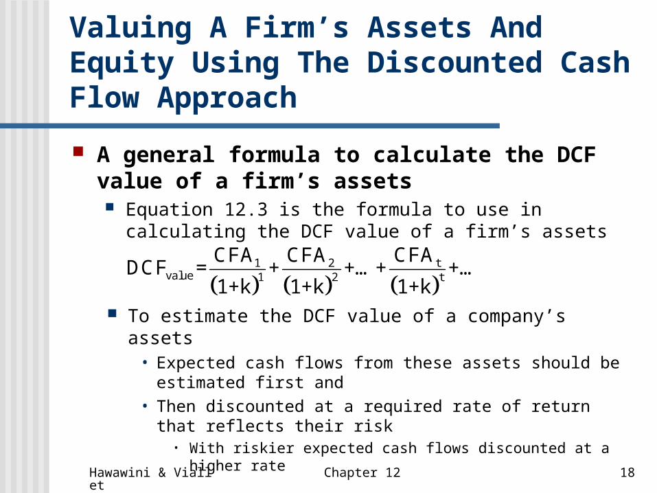
A general formula to calculate the DCF value of a firm’s assets Equation 12.3 is the formula to use in calculating the DCF value

of a firm’s assets


To estimate the DCF value of a company’s assets• Expected cash flows from these assets should be estimated first

and

• Then discounted at a required rate of return that reflects their risk• With riskier expected cash flows discounted at a higher rate

t1 2

value 1 2 t

CFACFA CFADCF = + +…+ +…

1+k 1+k 1+k


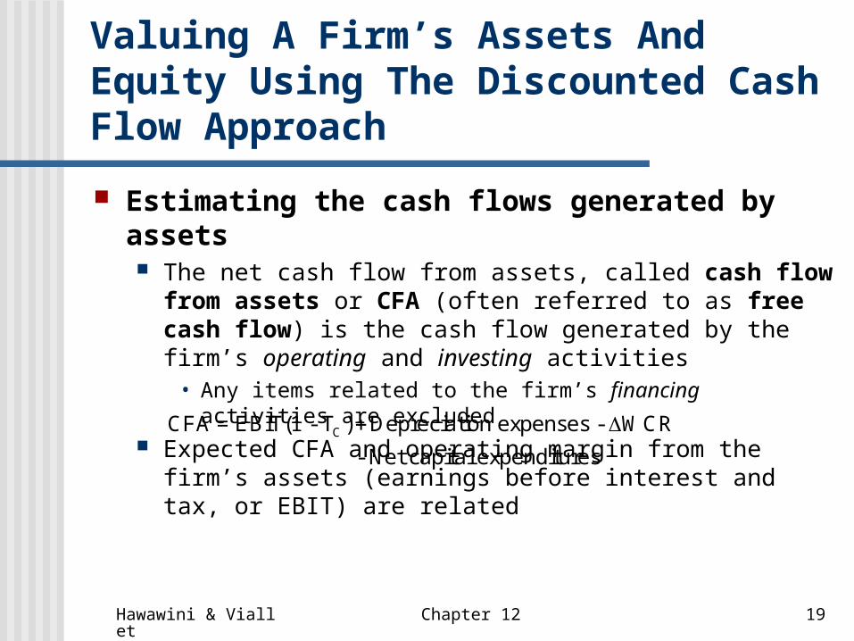
Estimating the cash flows generated by assets The net cash flow from assets, called cash flow from assets

or CFA (often referred to as free cash flow) is the cash flow generated by the firm’s operating and investing activities

• Any items related to the firm’s financing activities are excluded Expected CFA and operating margin from the firm’s assets

(earnings before interest and tax, or EBIT) are related


CCFA = EBIT(1 - T ) Depreciation expenses - WCR

- Net capital expenditures


Estimating the rate of return required to discount the cash flows The minimum required rate of return used to discount

the cash flows generated by assets must be at least equal to the cost of financing the assets

• Weighted average cost of capital (WACC) is the relevant discount rate


E D

equity debtWACC = k + k 1-tax rate

equity + debt equity + debt

• Capital asset pricing model (CAPM) is an approach to estimating the cost of equity financing

E Fk = R market risk premium β


Estimating The DCF Value Of A Firm’s Equity Buying the firm’s assets is not the same

as buying that firm’s equity If we buy a firm’s equity from its existing

owners, we will own the firm’s assets and we will also assume the firm’s existing debt

The estimated DCF value of a firm’s equity is the difference between the DCF value of its assets and the value of its outstanding debt


Estimating The DCF Value Of OS Distributors’ Assets And Equity

Example: Conducting a DCF valuation using the valuation of OS Distributors’ assets and equity Assumed that the firm will stay as is, i.e. its

operating efficiency remains the same as in 2000

Stand-alone value is estimated in a four-step procedure


Step 1: Estimation of OS Distributors’ cash flow from assets When estimating the DCF value of a firm’s assets,

the usual forecasting period is five years,• In the case of OS Distributors from 2001 to 2006

When a firm is valued as a going concern, we also need to estimate the terminal (or residual) DCF value of its assets, at the end of the forecasting period

• Value is based on the cash flows the firm’s assets are expected to generate beyond the forecasting period



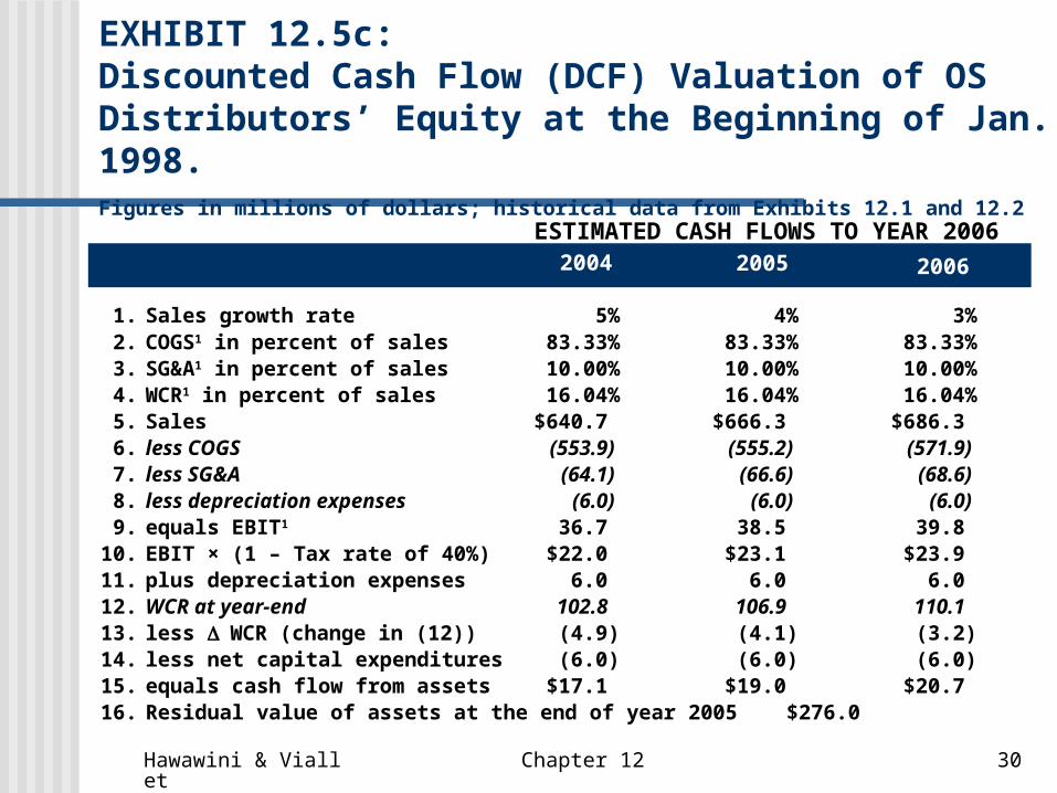
Estimating the cash flows from assets up to year 2006 The forecast of OS Distributors’ cash flows and their DCF value

are shown in Exhibit 12.5• Assumed that the growth rate will drop from 10 percent to a

residual level of 3 percent at the end of the forecast period• After the growth rates are estimated, expenses are calculated as a

percentage of sales• Since OS Distributors is valued as is, no major investments are

expected beyond the maintenance of existing assets• Maintenance costs are assumed to be exactly the same as the

annual depreciation expenses• Issue of consistency in making forecasts

• For example, if the firm’s activities are assumed to slow down, so should its capital expenditure and depreciation expenses



Estimating the residual value of assets at the end of year 2005 Use the constant growth formula to estimate

the residual value of OS Distributors’ assets at the end of year 2005

• The firm’s rate of growth in perpetuity after the year 2006 is the residual level of 3 percent, the estimated secular growth rate of the entire economy

• WACC is the one estimated in step 2



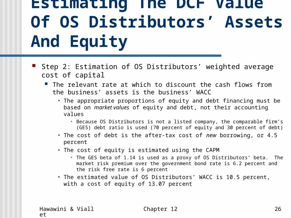
Step 2: Estimation of OS Distributors’ weighted average cost of capital The relevant rate at which to discount the cash flows from the

business’ assets is the business’ WACC• The appropriate proportions of equity and debt financing must be based on

market values of equity and debt, not their accounting values• Because OS Distributors is not a listed company, the comparable firm’s (GES)

debt ratio is used (70 percent of equity and 30 percent of debt)

• The cost of debt is the after-tax cost of new borrowing, or 4.5 percent• The cost of equity is estimated using the CAPM

• The GES beta of 1.14 is used as a proxy of OS Distributors’ beta. The market risk premium over the government bond rate is 6.2 percent and the risk free rate is 6 percent

• The estimated value of OS Distributors’ WACC is 10.5 percent, with a cost of equity of 13.07 percent



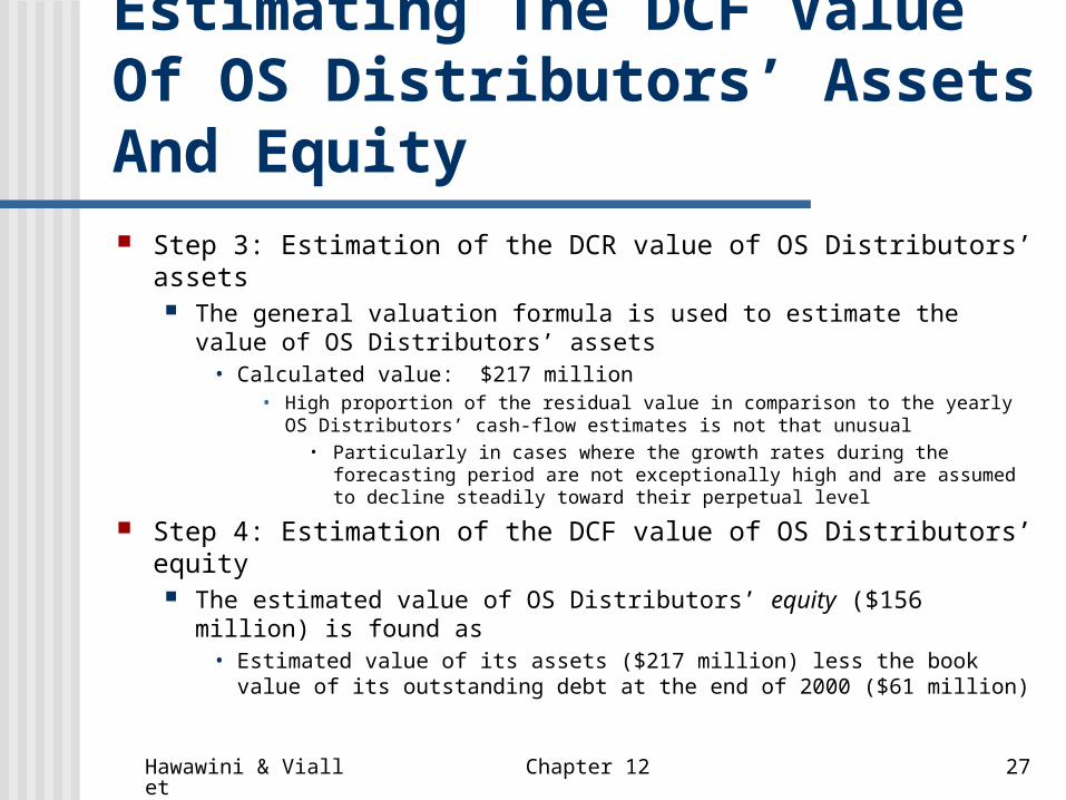
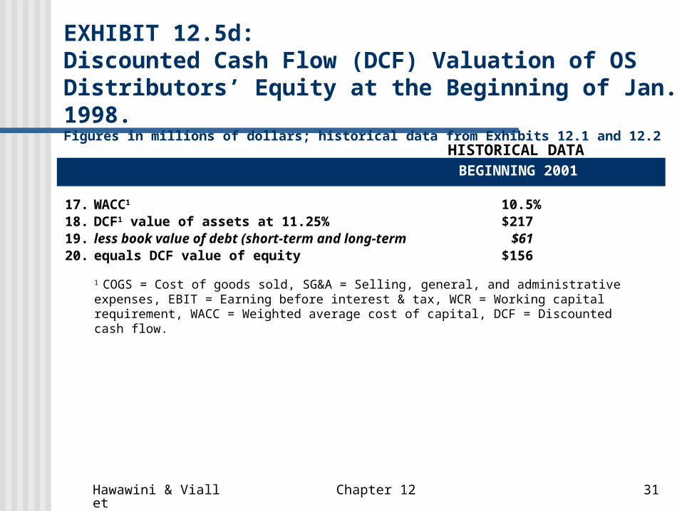
Step 3: Estimation of the DCR value of OS Distributors’ assets The general valuation formula is used to estimate the value of OS

Distributors’ assets• Calculated value: $217 million

• High proportion of the residual value in comparison to the yearly OS Distributors’ cash-flow estimates is not that unusual

• Particularly in cases where the growth rates during the forecasting period are not exceptionally high and are assumed to decline steadily toward their perpetual level

Step 4: Estimation of the DCF value of OS Distributors’ equity The estimated value of OS Distributors’ equity ($156 million) is found

as • Estimated value of its assets ($217 million) less the book value of its

outstanding debt at the end of 2000 ($61 million)



EXHIBIT 12.5a: Discounted Cash Flow (DCF) Valuation of OS Distributors’ Equity at the Beginning of Jan. 2001.Figures in millions of dollars; historical data from Exhibits 12.1 and 12.2

1999 2000

1. Sales growth rate 7.7% 14.3%2. COGS1 in percent of sales 84.10% 84.05% 83.33%3. SG&A1 in percent of sales 10.21% 10.40% 10.00%4. WCR1 in percent of sales 15.13% 15.00% 16.04%5. Sales $390.0 $420.0 $480.06. less COGS (328.0) (353.0) (400.0)7. less SG&A (39.8) (43.7) (48.0)8. less depreciation expenses (5.0) (5.0) (8.0)9. equals EBIT1 17.2 18.3 24.0

10. EBIT × (1 – Tax rate of 40%) $10.3 $11.0 $14.411. plus depreciation expenses 5.0 5.0 8.012. WCR at year-end 59.0 63.0 77.013. less WCR (change in (12)) (4.0) (14.0)14. less net capital expenditures (0.0) (10.0)15. equals cash flow from assets –$1.616. Residual value of assets at the end of year 2005

1998

HISTORICAL DATA


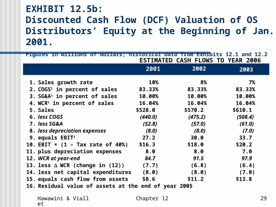
EXHIBIT 12.5b: Discounted Cash Flow (DCF) Valuation of OS Distributors’ Equity at the Beginning of Jan. 2001.Figures in millions of dollars; historical data from Exhibits 12.1 and 12.2

2002 2003

1. Sales growth rate 10% 8% 7%2. COGS1 in percent of sales 83.33% 83.33% 83.33%3. SG&A1 in percent of sales 10.00% 10.00% 10.00%4. WCR1 in percent of sales 16.04% 16.04% 16.04%5. Sales $528.0 $570.2 $610.16. less COGS (440.0) (475.2) (508.4)7. less SG&A (52.8) (57.0) (61.0)8. less depreciation expenses (8.0) (8.0) (7.0)9. equals EBIT1 27.2 30.0 33.7

10. EBIT × (1 – Tax rate of 40%) $16.3 $18.0 $20.211. plus depreciation expenses 8.0 8.0 7.012. WCR at year-end 84.7 91.5 97.913. less WCR (change in (12)) (7.7) (6.8) (6.4)14. less net capital expenditures (8.0) (8.0) (7.0)15. equals cash flow from assets $8.6 $11.2 $13.816. Residual value of assets at the end of year 2005

2001ESTIMATED CASH FLOWS TO YEAR 2006


EXHIBIT 12.5c: Discounted Cash Flow (DCF) Valuation of OS Distributors’ Equity at the Beginning of Jan. 1998.Figures in millions of dollars; historical data from Exhibits 12.1 and 12.2

2005 2006

1. Sales growth rate 5% 4% 3%2. COGS1 in percent of sales 83.33% 83.33% 83.33%3. SG&A1 in percent of sales 10.00% 10.00% 10.00%4. WCR1 in percent of sales 16.04% 16.04% 16.04%5. Sales $640.7 $666.3 $686.36. less COGS (553.9) (555.2) (571.9)7. less SG&A (64.1) (66.6) (68.6)8. less depreciation expenses (6.0) (6.0) (6.0)9. equals EBIT1 36.7 38.5 39.8

10. EBIT × (1 – Tax rate of 40%) $22.0 $23.1 $23.911. plus depreciation expenses 6.0 6.0 6.012. WCR at year-end 102.8 106.9 110.113. less WCR (change in (12)) (4.9) (4.1) (3.2)14. less net capital expenditures (6.0) (6.0) (6.0)15. equals cash flow from assets $17.1 $19.0 $20.716. Residual value of assets at the end of year 2005 $276.0

2004

ESTIMATED CASH FLOWS TO YEAR 2006


EXHIBIT 12.5d: Discounted Cash Flow (DCF) Valuation of OS Distributors’ Equity at the Beginning of Jan. 1998.Figures in millions of dollars; historical data from Exhibits 12.1 and 12.2

BEGINNING 2001

17. WACC1 10.5%18. DCF1 value of assets at 11.25% $21719. less book value of debt (short-term and long-term $6120. equals DCF value of equity $156

HISTORICAL DATA

1 COGS = Cost of goods sold, SG&A = Selling, general, and administrative expenses, EBIT = Earning before interest & tax, WCR = Working capital requirement, WACC = Weighted average cost of capital, DCF = Discounted cash flow.


Comparison Of DCF Valuation And Valuation By Comparables

The DCF value of OS Distributors’ equity is lower than any of the values estimated from comparable multiples The fair value of OS Distributors is probably

closer to the DCF value than to any of its comparable values

• Because DCF valuation is based on the projected cash flows from OS Distributors’ own assets

• Rather than on a mix of financial market and accounting data from another company (GES)


Estimating The Acquisition Value Of OS Distributors The DCF equity value determined as is does not take into account

any potential improvement in managing the firm Such improvements—usually expected when the firm is acquired by

another one—result in potential value creation When a firm acquires another one, the potential value creation is

shared between the acquirer and the target If we call takeover premium the portion going to the target

• Then the net present value of the investment made by the acquirer is the difference between the potential value creation and the takeover premium

To estimate the acquisition value of a firm, must first identify the potential sources of value creation in an acquisition If those sources are not present, such as in a conglomerate merger,

an acquisition is not likely to create value


Identifying The Potential Sources Of Value Creation In An Acquisition

In order to create value an acquisition must achieve one of the following: Increase the cash flows generated by the target firm’s assets Raise the growth rate of the target firm’s sales Lower the WACC of the target firm

Inefficient management and synergy provide the most powerful reasons to justify an acquisition Other reasons

• Undervaluation hypothesis

• Market power hypothesis



Specific sources of value creation in an acquisition Increasing the cash flows generated by the target

firm’s assets• A reduction in a firm’s cost of goods sold or in its selling,

general, and administrative expenses will increase its operating profits, thus increasing the firm’s cash flows

• A reduction in tax expenses will have the same effect

• Another way to increase the target firm’s cash flows is to use its assets more efficiently

• A more efficient use of assets can be achieved by reducing any over-investment (e.g. in cash, working capital requirement or in fixed assets)



Raising the sales growth rate• All other things being equal, faster growth in sales will

create additional value• Can be achieved by increasing the volume of goods or

services sold and/or by raising their price using superior marketing skills and strategies

Lowering the cost of capital• If the target firm’s capital structure is currently not close to

its optimal level, then changing the firm’s capital structure when the firm is acquired should lower its WACC and raise its value



A merger is unlikely to lead to a reduction in the cost of equity Often argued that if the merged firms are perceived

by their creditors to be less likely to fail as a combination than as separate entities

• Then their post-merger cost of debt could be lower (coinsurance effect)


Why Conglomerate Mergers Are Unlikely To Create Lasting Value Through Acquisition

Conglomerate merger may increase the conglomerate’s earnings per share (EPS) But the growth in EPS is unlikely to be accompanied

by a permanent rise in shareholder value• Acquiring unrelated businesses is unlikely to create

lasting value• May make sense from the perspective of the acquirer’s

managers, but it is unlikely to create value • Since investors can generate the same value by

combining shares of the two companies in their personal portfolios (homemade diversification)

• Only types of mergers that are likely to create lasting value are those that result in managerial improvements or synergistic gains (i.e. horizontal or vertical mergers)


Why Conglomerate Mergers Are Unlikely To Create Lasting Value Through Acquisition

• Raising earnings per share through conglomerate mergers is unlikely to create lasting value

• Some conglomerates grow rapidly by continuously buying firms that have a lower price-to-earnings (P/E) ratio than the P/E of the conglomerate firm, on the premise that

• Market will value the combination for more than the sum of the pre-merger firms


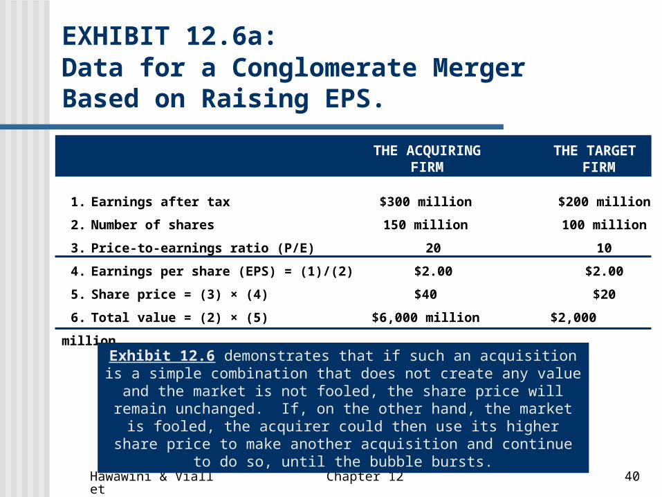
EXHIBIT 12.6a: Data for a Conglomerate Merger Based on Raising EPS.

THE ACQUIRING FIRM

THE TARGET FIRM

1. Earnings after tax $300 million $200 million

2. Number of shares 150 million 100 million

3. Price-to-earnings ratio (P/E) 20 10

4. Earnings per share (EPS) = (1)/(2) $2.00 $2.00

5. Share price = (3) × (4) $40 $20

6. Total value = (2) × (5) $6,000 million $2,000 million

Exhibit 12.6 demonstrates that if such an acquisition is a simple combination that does not create any value and the market is not fooled, the share price will remain unchanged. If, on the other hand, the market

is fooled, the acquirer could then use its higher share price to make another acquisition and continue to do so, until the bubble bursts.


EXHIBIT 12.6b: Data for a Conglomerate Merger Based on Raising EPS.

IS VALUE NEUTRAL

EXCEEDS VALUE NEUTRALITY

1. Earnings after tax $500 million $500 million

2. Number of shares 200 million 200 million

3. Price-to-earnings ratio (P/E) 16 18

4. Earnings per share (EPS) = (1)/(2) $2.50 $2.50

5. Share price = (3) × (4) $40 $45

6. Total value = (2) × (5) $8,000 million $9,000 million

VALUE OF THE MERGED FIRM IF THE MARKET ASSIGNS THE COMBINATION A P/E THAT


The Acquisition Value Of OS Distributors’ Equity

To consider OS Distributors an acquisition target Potential acquirer first would have to determine that OS Distributors’

performance could be improved Assume that a prospective acquirer of OS Distributors has identified four

separate improvements that would result in a potential value creation Reduction in cost of goods sold Reduction in administrative and selling expenses More efficient management of the operating cycle Faster growth

• The value impact of those improvements is presented in Exhibits 12.7, 12.8, and 12.9

Overconfidence about the acquirer’s ability to realize the full potential of a target often leads to paying too much for the target Almost all of the gains from the acquisition end up in the pockets of the target

company’s shareholders


EXHIBIT 12.9: Summary of Data in Exhibits 12.7 and 12.8.

POTENTIAL VALUE CREATION

1. Reduction in the cost of goods sold to82.33% of sales $42 million (39%)

2. Reduction in overheads to 9.50% of sales $21 million (20%)

3. Reduction of working capital requirementto 13% of sales $22 million (21%)

4. Faster growth in sales (2 percentagepoints higher) $14 million (13%)

5. Interaction of growth and improvedoperations $8 million ( 7%)

Total potential value creation $107 million (100%)

SOURCES OF VALUE CREATION


Estimating The Leveraged Buyout Value Of OS Distributors In a typical leveraged buyout (LBO)

Group of investors purchases a presumably underperforming firm by raising an unusually large amount of debt relative to equity funding

Assume that the top managers of OS Distributors buy the firm from the current owner for $200 million Financed by $160 million of debt and $40 million of equity

Exhibit 12.10 compares OS Distributors’ balance sheets before and after the LBO Key issues regarding the LBO of OS Distributors are:

• Whether the acquisition is a value-creating investment• Whether the acquired assets will generate sufficient cash to

service the LBO loan


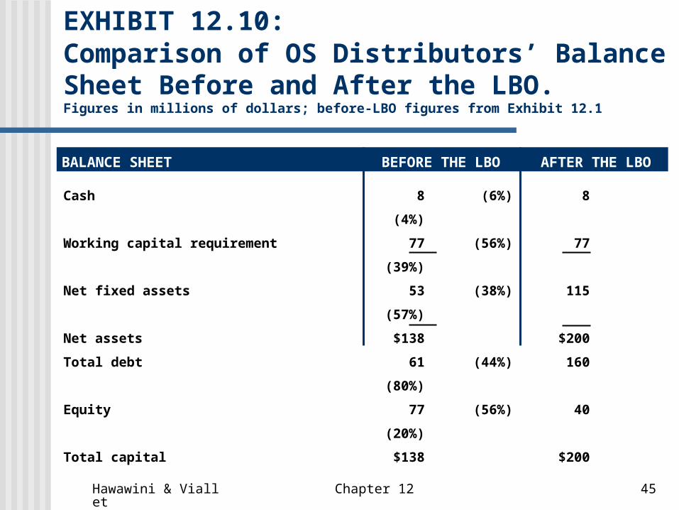
EXHIBIT 12.10: Comparison of OS Distributors’ Balance Sheet Before and After the LBO.Figures in millions of dollars; before-LBO figures from Exhibit 12.1

BEFORE THE LBO

Cash 8 (6%) 8

(4%)

Working capital requirement 77 (56%) 77

(39%)

Net fixed assets 53 (38%) 115

(57%)

Net assets $138 $200

Total debt 61 (44%) 160

(80%)

Equity 77 (56%) 40

(20%)

Total capital $138 $200

AFTER THE LBOBALANCE SHEET


Estimating The Leveraged Buyout Value Of OS Distributors Equity

DCF approach assumes that the WACC will remain constant Not the case in an LBO, where a large portion of the

corresponding loan is repaid over just a few years• This problem is circumvented using the adjusted present

value (APV) method• The adjusted present value method

• DCF value of a firm’s assets is first estimated assuming they are not financed with debt

• Then DCF value of future tax savings due to borrowing, estimated by discounting the future stream of tax savings at the cost of debt, is added


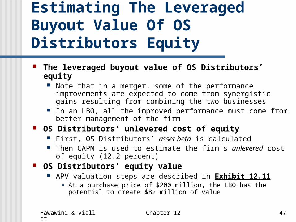
Estimating The Leveraged Buyout Value Of OS Distributors Equity The leveraged buyout value of OS Distributors’ equity

Note that in a merger, some of the performance improvements are expected to come from synergistic gains resulting from combining the two businesses

In an LBO, all the improved performance must come from better management of the firm

OS Distributors’ unlevered cost of equity First, OS Distributors’ asset beta is calculated Then CAPM is used to estimate the firm’s unlevered cost of equity

(12.2 percent) OS Distributors’ equity value

APV valuation steps are described in Exhibit 12.11• At a purchase price of $200 million, the LBO has the potential to create $82

million of value


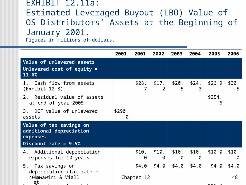
EXHIBIT 12.11a:Estimated Leveraged Buyout (LBO) Value of OS Distributors’ Assets at the Beginning of January 2001.Figures in millions of dollars.

2001 2001 2002 2003 2004 2005 2006

Value of unlevered assets

Unlevered cost of equity = 11.6%

1. Cash flow from assets (Exhibit 12.8) $28.7 $17.2 $20.5 $24.3 $26.9 $30.5

2. Residual value of assets at end of year 2005

$354.6

3. DCF value of unlevered assets $290.0

Value of tax savings on additional depreciation expenses

Discount rate = 9.5%

4. Additional depreciation expenses for 10 years

$10.0 $10.0 $10.0 $10.0 $10.0 $10.0

5. Tax savings on depreciation (tax rate = 40%)

$4.0 $4.0 $4.0 $4.0 $4.0 $4.0

6. Residual value of tax savings $15.4

7. DCF value of tax savings from deprecation

$25.1


EXHIBIT 12.11a:Estimated Leveraged Buyout (LBO) Value of OS Distributors’ Assets at the Beginning of January 2001.Figures in millions of dollars.

2001 2001 2002 2003 2004 2005 2006

Value of tax savings on interest expenses

Cost of debt = 9.5%

8. Debt outstanding at the beginning of the year

$160.0 $145.0 $130.0 $115.0 $100.0 $85.0

9. Debt repayment $15.0 $15.0 $15.0 $15.0 $15.0

10. Debt outstanding at the end of the year $145.0 $130.0 $115.0 $100.0 $85.0 $87.6

11. Interest Expenses (interest rate = 9.5%) $15.2 $13.2 $12.4 $10.9 $9.5 $8.3

12. Tax savings on interest expenses (tax rate = 40%)

$6.1 $5.5 $5.0 $4.4 $3.8 $3.3

13. Residual value of tax savings $50.8

14. DCF value of tax savings from interest expenses

$51.7

15. DCF value of overall tax savings (7+14) $76.8

16. DCF value of levered assets 3+15 $366.8


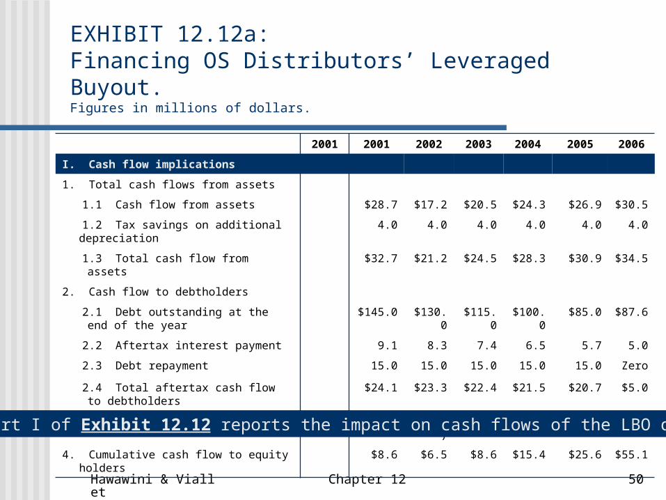
EXHIBIT 12.12a:Financing OS Distributors’ Leveraged Buyout.Figures in millions of dollars.

2001 2001 2002 2003 2004 2005 2006

I. Cash flow implications

1. Total cash flows from assets

1.1 Cash flow from assets $28.7 $17.2 $20.5 $24.3 $26.9 $30.5

1.2 Tax savings on additional depreciation 4.0 4.0 4.0 4.0 4.0 4.0

1.3 Total cash flow from assets $32.7 $21.2 $24.5 $28.3 $30.9 $34.5

2. Cash flow to debtholders

2.1 Debt outstanding at the end of the year $145.0 $130.0 $115.0 $100.0 $85.0 $87.6

2.2 Aftertax interest payment 9.1 8.3 7.4 6.5 5.7 5.0

2.3 Debt repayment 15.0 15.0 15.0 15.0 15.0 Zero

2.4 Total aftertax cash flow to debtholders $24.1 $23.3 $22.4 $21.5 $20.7 $5.0

3. Cash flow to equity holders $8.6 ($2.1) $2.1 $6.8 $10.2 $29.5

4. Cumulative cash flow to equity holders $8.6 $6.5 $8.6 $15.4 $25.6 $55.1

Part I of Exhibit 12.12 reports the impact on cash flows of the LBO deal.


2001 2001 2002 2003 2004 2005 2006

II. Pro forma income statements

Earnings before interest and tax (EBIT) $24.0 $35.9 $40.3 $45.7 $50.4 $53.7 $55.5

Additional depreciation (0) (10.0) (10.0) (10.0) (10.0) (10.0) (10.0)

Interest expenses (7.0) (15.2) (13.8) (12.4) (10.9) (9.5) (8.3)

Earnings before tax (EBT) $17.0 $10.7 $16.5 $23.3 $29.5 $34.2 $37.2

Tax (40%) (6.8) (4.3) (6.6) (9.3) (11.8) (13.7) (14.9)

Earnings after tax (EAT) $10.2 $6.4 $9.9 $14.0 $17.7 $20.5 $22.3

III. Capital and debt ratios

Debt outstanding (from above) $61.0 $145.0 $130.0 $115.0 $100.0 $85.0 $87.6

Equity capital $77.0 $46.4 $56.3 $70.3 $88.0 $108.5 $130.8

Total capital $138.0 $191.4 $186.3 $185.3 $188.0 $193.5 $218.4

Ratio of debt to total capital 44% 76% 70% 62% 53% 44% 40%

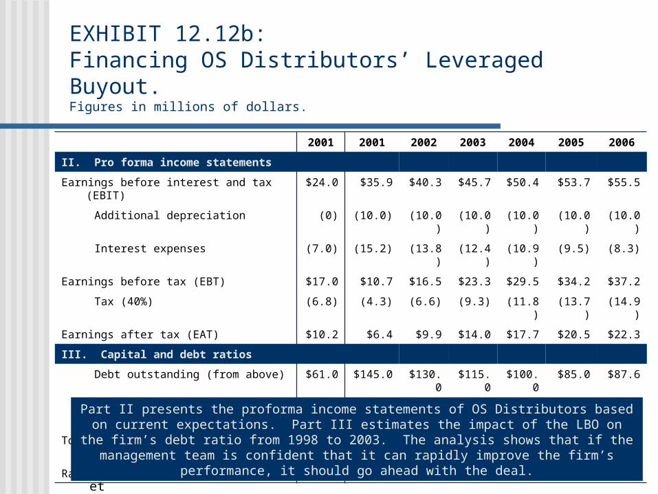
EXHIBIT 12.12b:Financing OS Distributors’ Leveraged Buyout.Figures in millions of dollars.

Part II presents the proforma income statements of OS Distributors based on current expectations. Part III estimates the impact of the LBO on the firm’s debt ratio from 1998 to 2003. The analysis shows that if the management team is confident that it can rapidly improve the firm’s

performance, it should go ahead with the deal.


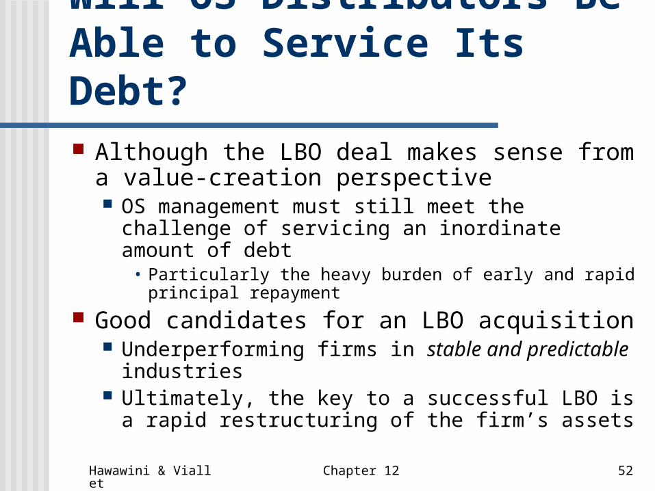
Will OS Distributors Be Able to Service Its Debt? Although the LBO deal makes sense from a

value-creation perspective OS management must still meet the challenge of

servicing an inordinate amount of debt• Particularly the heavy burden of early and rapid principal

repayment

Good candidates for an LBO acquisition Underperforming firms in stable and predictable

industries Ultimately, the key to a successful LBO is a rapid

restructuring of the firm’s assets


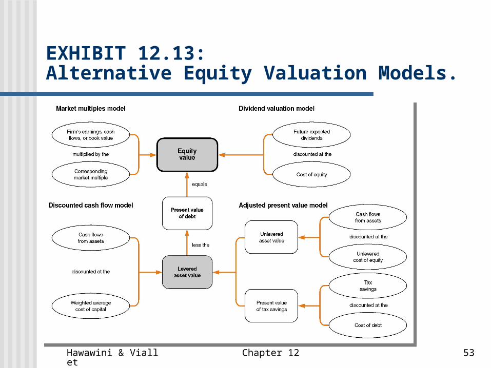
EXHIBIT 12.13: Alternative Equity Valuation Models.

hawawini & vialletchapter 121 valuing and acquiring a business

Documents

market value

business value

equity value

expectedthe value

business chapter

comparable firms

comparable market multiples

os distributors balance