Proceedings of the Tenth Pacific Conference on Earthquake Engineering

Building an Earthquake-Resilient Pacific

6-8 November 2015, Sydney, Australia

Paper Number 212

Hazard Identification and Behaviour of Reinforced Concrete Framed

Buildings in Regions of Lower Seismicity

Wilson JL1, Lam NTK2, Gad EF1

1. Swinburne University of Technology, Hawthorn, Victoria, Australia

2. University of Melbourne, Parkville, Victoria, Australia.

Abstract

Soft storey buildings are common in regions of lower seismicity and are considered particularly

vulnerable due to their limited displacement capacity. This paper presents a displacement based

(DB) method for assessing limited ductile R/C frame buildings and particularly soft storey

buildings. The paper addresses both the challenges of defining hazard levels in lower seismic

regions and developing representative load-drift curves for limited ductile columns. The

displacement demand in regions of lower seismicity are typically modest and in the range of

20-100mm depending on the soil conditions and the return period event. The displacement

capacity of lightly reinforced concrete columns is not well understood and a detailed and

simplified model for estimating the load-drift behaviour is presented. The detailed model

clearly indicates the dramatic impact that the axial load ratio has on the drift performance of

lightly reinforced columns with the drift capacity reducing from 5.0% to 1.0% for compression

dominated columns.

Keywords: Drift capacity, axial load ratio, limited ductile columns, soft storeys, hazard

estimates, intraplate seismicity, seismic performance, displacement based

1. Introduction

Studies undertaken by the authors in recent years have indicated that the existing building stock

at most risk of damage and collapse from earthquake excitation in lower seismicity regions such

as Australia are unreinforced masonry buildings and reinforced concrete frame buildings that

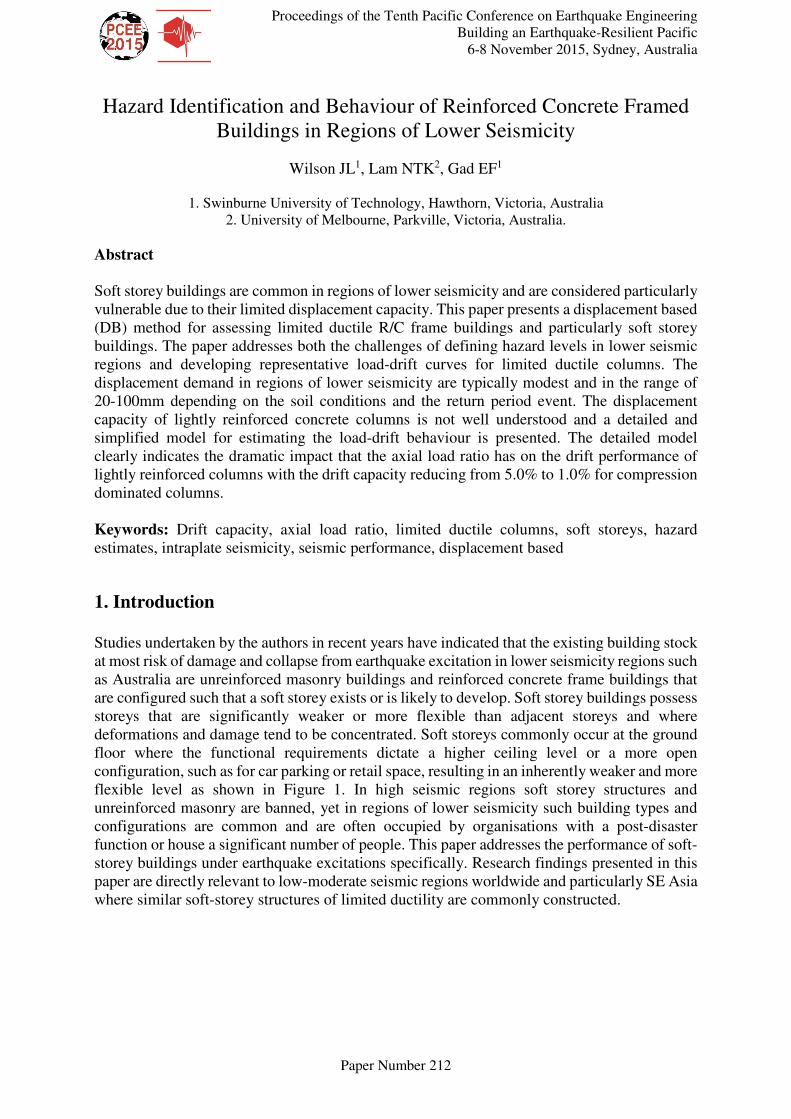
are configured such that a soft storey exists or is likely to develop. Soft storey buildings possess

storeys that are significantly weaker or more flexible than adjacent storeys and where

deformations and damage tend to be concentrated. Soft storeys commonly occur at the ground

floor where the functional requirements dictate a higher ceiling level or a more open

configuration, such as for car parking or retail space, resulting in an inherently weaker and more

flexible level as shown in Figure 1. In high seismic regions soft storey structures and

unreinforced masonry are banned, yet in regions of lower seismicity such building types and

configurations are common and are often occupied by organisations with a post-disaster

function or house a significant number of people. This paper addresses the performance of soft-

storey buildings under earthquake excitations specifically. Research findings presented in this

paper are directly relevant to low-moderate seismic regions worldwide and particularly SE Asia

where similar soft-storey structures of limited ductility are commonly constructed.

2

Figure 1 Typical soft storey buildings

Soft-storey buildings are considered to be particularly vulnerable because the rigid block at the

upper levels has limited energy absorption and displacement capacity, thus leaving the columns

in the soft-storey to deflect and absorb the seismic energy. Collapse of the building is imminent

when the energy absorption capacity or displacement capacity of the soft-storey columns is

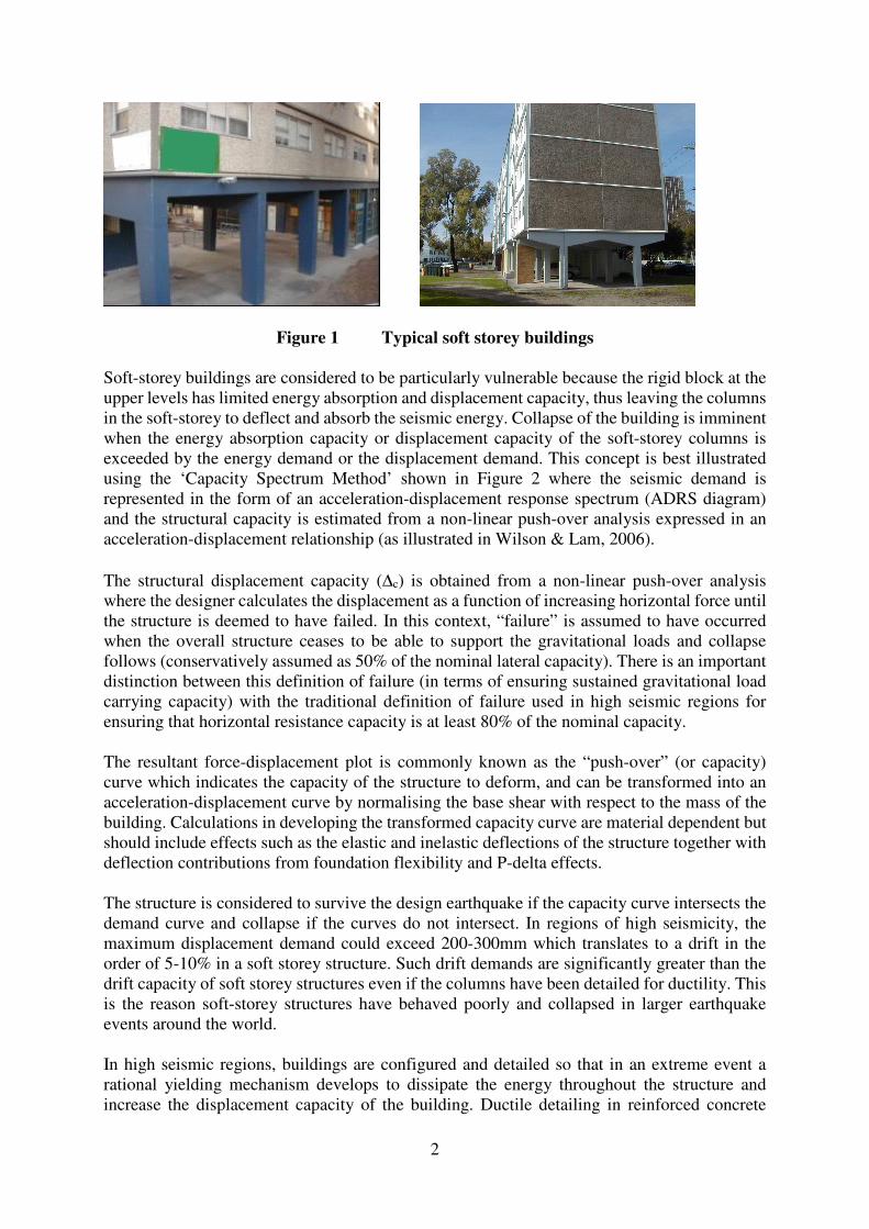
exceeded by the energy demand or the displacement demand. This concept is best illustrated

using the ‘Capacity Spectrum Method’ shown in Figure 2 where the seismic demand is

represented in the form of an acceleration-displacement response spectrum (ADRS diagram)

and the structural capacity is estimated from a non-linear push-over analysis expressed in an

acceleration-displacement relationship (as illustrated in Wilson & Lam, 2006).

The structural displacement capacity (∆c) is obtained from a non-linear push-over analysis

where the designer calculates the displacement as a function of increasing horizontal force until

the structure is deemed to have failed. In this context, “failure” is assumed to have occurred

when the overall structure ceases to be able to support the gravitational loads and collapse

follows (conservatively assumed as 50% of the nominal lateral capacity). There is an important

distinction between this definition of failure (in terms of ensuring sustained gravitational load

carrying capacity) with the traditional definition of failure used in high seismic regions for

ensuring that horizontal resistance capacity is at least 80% of the nominal capacity.

The resultant force-displacement plot is commonly known as the “push-over” (or capacity)

curve which indicates the capacity of the structure to deform, and can be transformed into an

acceleration-displacement curve by normalising the base shear with respect to the mass of the

building. Calculations in developing the transformed capacity curve are material dependent but

should include effects such as the elastic and inelastic deflections of the structure together with

deflection contributions from foundation flexibility and P-delta effects.

The structure is considered to survive the design earthquake if the capacity curve intersects the

demand curve and collapse if the curves do not intersect. In regions of high seismicity, the

maximum displacement demand could exceed 200-300mm which translates to a drift in the

order of 5-10% in a soft storey structure. Such drift demands are significantly greater than the

drift capacity of soft storey structures even if the columns have been detailed for ductility. This

is the reason soft-storey structures have behaved poorly and collapsed in larger earthquake

events around the world.

In high seismic regions, buildings are configured and detailed so that in an extreme event a

rational yielding mechanism develops to dissipate the energy throughout the structure and

increase the displacement capacity of the building. Ductile detailing in reinforced concrete

3

columns includes closely spaced closed stirrups to confine the concrete, prevent longitudinal

steel buckling and to increase the shear capacity of columns (Mander, 1988; Park, 1997; Paulay

& Priestley, 1992). The emphasis is on the prevention of brittle failure modes and the

encouragement of ductile mechanisms through the formation of plastic hinges that can rotate

without strength degradation to create the rational yielding mechanism.

Current detailing practice in the regions of lower seismicity typically allow widely spaced

stirrups (typical stirrup spacing in the order of the minimum column dimension) resulting in

concrete that is not effectively confined to prevent crushing and spalling, longitudinal steel that

is not prevented from buckling and columns that are weaker in shear. Design guidelines that

have been developed in regions of high seismicity (ATC40, FEMA273) recommend a very low

drift capacity for columns that have such a low level of detailing. The application of such

standards in the context of low-moderate seismicity regions results in most soft-storey

structures being deemed to fail when subject to the earthquake event consistent with a return

period in the order of 500 – 1500 years. Previous studies by the authors have confirmed the

conservative nature of these guidelines (Wibowo et al 2009, Wilson et al 2009).

Figure 2 Capacity spectrum method

The overall aim of this paper is to present a methodology that can be used to assess the seismic

performance of lightly reinforced concrete soft storey structures. Section 2 presents the seismic

demand in regions of lower seismicity including a discussion on displacement controlled

behaviour and probabilistic hazard analysis, whilst Section 3 presents push-over curves for a

range of lightly reinforced concrete columns using both detailed and simplified models. The

resulting demand and capacity curves can be overlaid using the Capacity Spectrum Method

(CSM) as illustrated in Figure 2 and summarised in Section 4.

2. Seismic Displacement Demand

2.1 General

The current force-based design guidelines are founded on the concept of trading strength for

ductility to ensure the structure has sufficient energy absorbing capacity. The developing

displacement-based (DB) design methodologies may also be calibrated to fulfill this objective

more elegantly (eg. Priestley et al, 2007 & 2011; Wilson & Lam, 2006). In each load-cycle, the

amount of energy absorbed is equal to the integral product of the resisting force (strength) and

4

deformation (“ductility”). This approach assumes that the imposed kinetic energy does not

subside during the displacement response of the building which is not unreasonable in regions

of high seismicity where the earthquake magnitudes are larger and the duration of ground

shaking longer. The limitation of this approach in lower seismic regions is examined herein

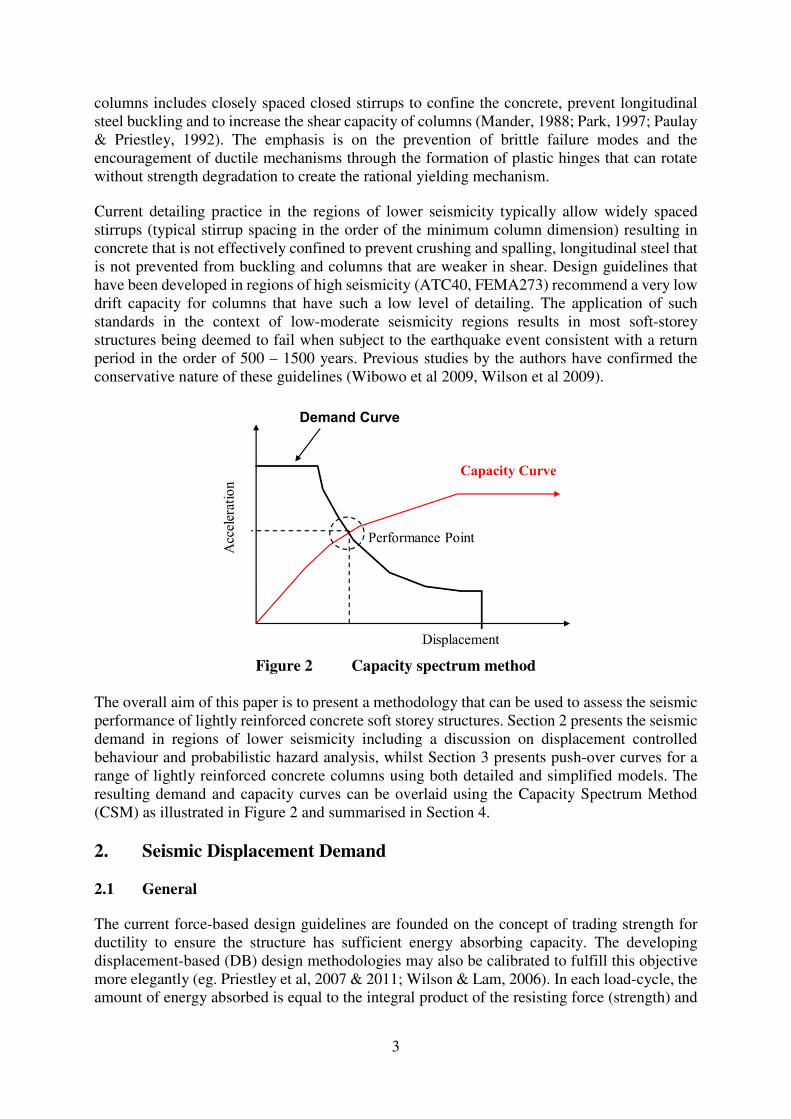
with the idealized pulses shown in Figure 3.

The velocity developed in an elastic single-degree-of-freedom system would increase with

increasing natural period (T) until T approaches the pulse duration (td) when maximum velocity

is developed. Importantly, as T continues to increase, the velocity demand subsides while the

displacement levels-off to a value constrained by the peak ground displacement (PGD). It is

hypothesized that this phenomenon of displacement-controlled behaviour can be extended to

inelastically responding systems in which case T/2 corresponds to the time taken by the

structure to load-and-unload.

(a) Ground displacement pulse

(b )Velocity response spectrum (c) Displacement response spectrum

Figure 3 Displacement and velocity response spectra from a pulse

The single-pulse scenario, despite its simplicity (which is convenient for illustration), has been

used in formal evaluations to quantify the seismic demand of the more complex pulse trains in

small and moderate magnitude earthquakes on rock sites in intraplate regions (Lam & Chandler,

2005). However, on some soft soil sites, the displacement demand of periodic pulses on the

structure can be many times higher than the PGD when conditions pertaining to soil resonance

behaviour are developed. Even then, the peak displacement demand on the structure is well

constrained around a definitive upper limit.

Research undertaken by the authors (eg. Lam et al, 2000a-c, 2001, 2003; Lam & Wilson, 2004;

Wilson & Lam, 2003 & 2006; Lam & Chandler, 2004) has culminated in the drafting of the

new Standard for earthquake actions for Australia which incorporates this important upper

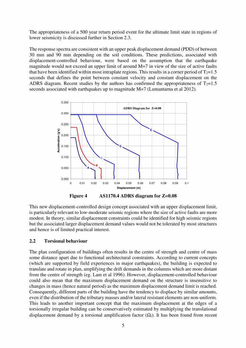
displacement demand limit (AS1170.4-2007). The AS1170.4 response spectra scaled for a 500

year return period hazard factor of Z=0.08g (which corresponds to a notional peak ground

velocity of PGV=60 mm/sec) has been plotted in Figure 4 for different site classes A-E (hard

rock to very soft soil) in an ADRS format (acceleration-displacement response spectra format).

0

0.008

0.016

0.024

0.032

0.04

0 1 2 3 4

Period (secs)

Ve

loc

ity

(m

/se

c)

0

0.002

0.004

0.006

0.008

0.01

0.012

0 1 2 3 4

Period (secs)

Dis

pla

ce

me

nt

(m)

Ground Displacement

(td = 2sec)

Displacement response

(T = 2 sec)

Demand subsides

with increasing

period

Displacement

upper limit

-0.015

-0.01-0.005

00.005

0.010.015

0 1 2 3 4 5 6 7 8 9

Time (secs)

Dis

pla

cem

en

t (m

)

5

The appropriateness of a 500 year return period event for the ultimate limit state in regions of

lower seismicity is discussed further in Section 2.3.

The response spectra are consistent with an upper peak displacement demand (PDD) of between

30 mm and 90 mm depending on the soil conditions. These predictions, associated with

displacement-controlled behaviour, were based on the assumption that the earthquake

magnitude would not exceed an upper limit of around M=7 in view of the size of active faults

that have been identified within most intraplate regions. This results in a corner period of T2=1.5

seconds that defines the point between constant velocity and constant displacement on the

ADRS diagram. Recent studies by the authors has confirmed the appropriateness of T2=1.5

seconds associated with earthquakes up to magnitude M=7 (Lumantarna et al 2012).

Figure 4 AS1170.4 ADRS diagram for Z=0.08

This new displacement-controlled design concept associated with an upper displacement limit,

is particularly relevant to low-moderate seismic regions where the size of active faults are more

modest. In theory, similar displacement constraints could be identified for high seismic regions

but the associated larger displacement demand values would not be tolerated by most structures

and hence is of limited practical interest.

2.2 Torsional behaviour

The plan configuration of buildings often results in the centre of strength and centre of mass

some distance apart due to functional architectural constraints. According to current concepts

(which are supported by field experiences in major earthquakes), the building is expected to

translate and rotate in plan, amplifying the drift demands in the columns which are more distant

from the centre of strength (eg. Lam et al 1996). However, displacement-controlled behaviour

could also mean that the maximum displacement demand on the structure is insensitive to

changes in mass (hence natural period) as the maximum displacement demand limit is reached.

Consequently, different parts of the building have the tendency to displace by similar amounts,

even if the distribution of the tributary masses and/or lateral resistant elements are non-uniform.

This leads to another important concept that the maximum displacement at the edges of a

torsionally irregular building can be conservatively estimated by multiplying the translational

displacement demand by a torsional amplification factor (Ωt). It has been found from recent

0.000

0.050

0.100

0.150

0.200

0.250

0.300

0.350

0 0.01 0.02 0.03 0.04 0.05 0.06 0.07 0.08 0.09 0.1

Displacement (m)

Acc

ele

rati

on

(g

's)

AB

C

D

E

ADRS Diagram for Z=0.08

6

research that this amplification factor is limited a value of Ωt=1.6 by displacement-controlled

behaviour (Lumantarna et al, 2013).

2.3 Probabilistic Hazard Analysis

Contemporary codes of practice for the earthquake design of structures generally use

probability seismic hazard analysis (PSHA) to account for the uncertainty in the level of ground

motion expected at a site. The probability of exceedance or return period (RP) associated with

a design event at a site requires a balance between cost and risk and is usually established and

recommended by Government authorities. The PHSA procedure uses historical data and trends

to predict the occurrence of future potentially destructive seismic events. Clearly such

predictions would only be realistic if the period of observation is sufficiently long to capture

the underlying seismic processes which are responsible for future events. The PSHA

methodology and return period selection is well established for regions of high seismicity, but

is much more difficult for regions of lower seismicity such as Australia, where there is a paucity

of data and no tectonic model to guide the process.

In Australia, the Australian Building Control Board (ABCB) have recommended a probability

of exceedance of 10% in 50 years for the ultimate limit state (ULS) design of normal structures,

which correlates with a return period (RP) of 475 years, which is commonly rounded off to 500

years. At the ULS, it is expected that the facility maybe heavily damaged but would not

collapse, with the emphasis on life protection rather than building damage avoidance. Such

return periods are considered reasonable for high seismic regions where the maximum credible

earthquake event could be expected to occur during this period. However, in regions of lower

seismicity, such as Australia, much greater ground shaking could occur from rarer events with

a much higher return period. The seismicity in Australia is not dissimilar to the eastern parts of

North America, where in countries such as Canada, authorities have set a return period of 2500

years for the design of structures to resist earthquake ground shaking.

The recent series of earthquakes in Christchurch, NZ, have highlighted the extreme

consequences of earthquakes that exceed the nominal 500 year design earthquake predicted

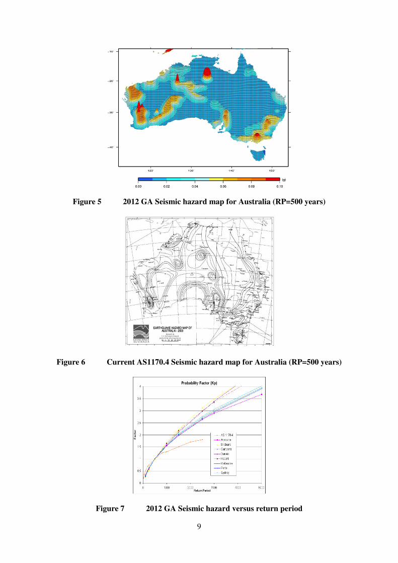
from PSHA studies. This issue has been highlighted further with the release of Geoscience

Australia’s updated earthquake hazard map for Australia in November 2012, which reduced the

seismic hazard for a 500 year RP event but significantly increased the hazard for RP greater

than 1500 years (Leonard et al 2013). The map has been developed thoroughly using the latest

science and complex modelling techniques applied to a sparse data set, resulting in a map that

is dominated by recent past earthquake events that appear as ‘hotspots’. The updated hazard

map is shown in Figure 5 where the hazard is represented by an effective peak ground

acceleration or ‘Z’ factor. The map is not based on a tectonic model that is typically developed

for high seismic regions with a certain degree of confidence and certainty. Consequently, the

hazard map developed for low seismic regions such as Australia has significant uncertainty,

since past events are not necessarily good predictors of future events. An example of this is a

location near Tennant Creek that experienced three M6.2-6.5 events on one day in January

1988, but before that was considered a region of very low seismicity and tectonically stable.

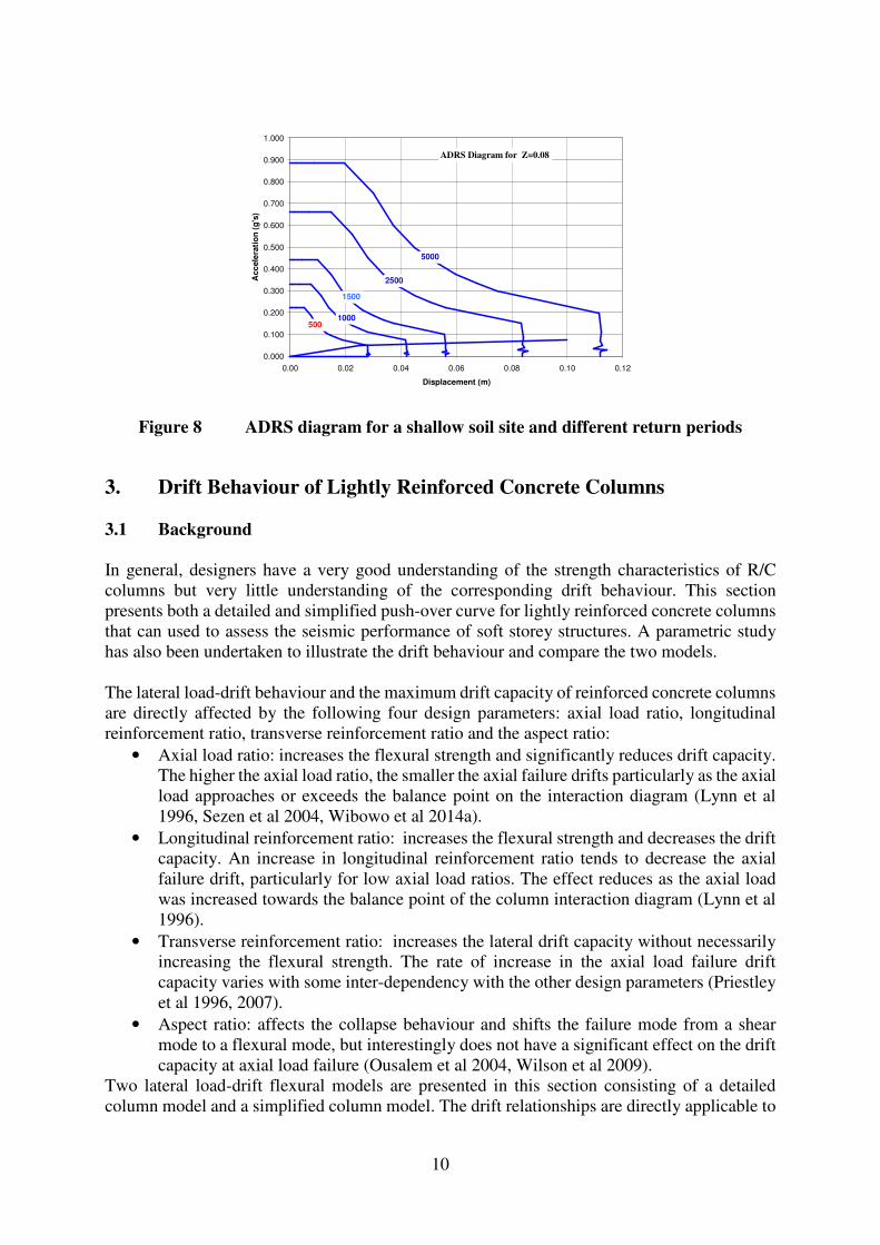
The 500 year RP seismicity levels in the GA 2012 hazard map are generally less than the hazard

map values in the current Australian Earthquake Loading Standard AS1170.4 (2007), which

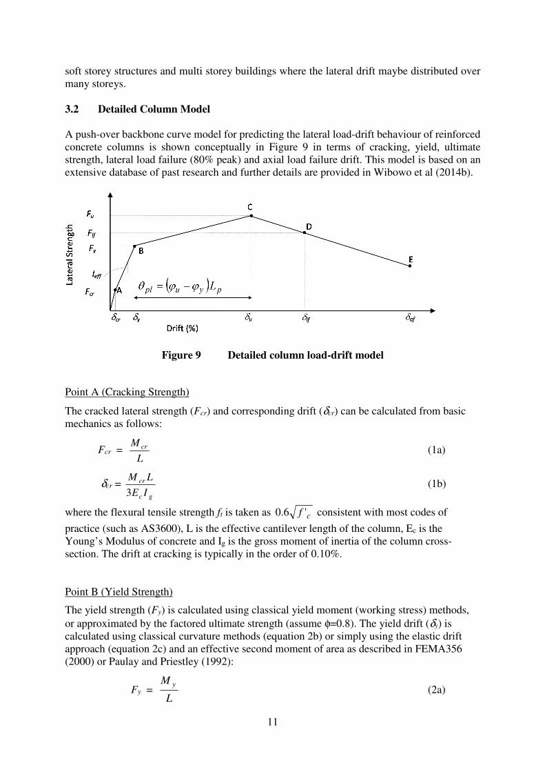
were developed by GA in the late 1980s and shown in Figure 6. However, the 2012 GA updated

probability factors for adjusting the 500 year RP values for longer RP events are greater than

the current published values in AS1170.4 as shown in Figure 7. This is illustrated in Table 1,

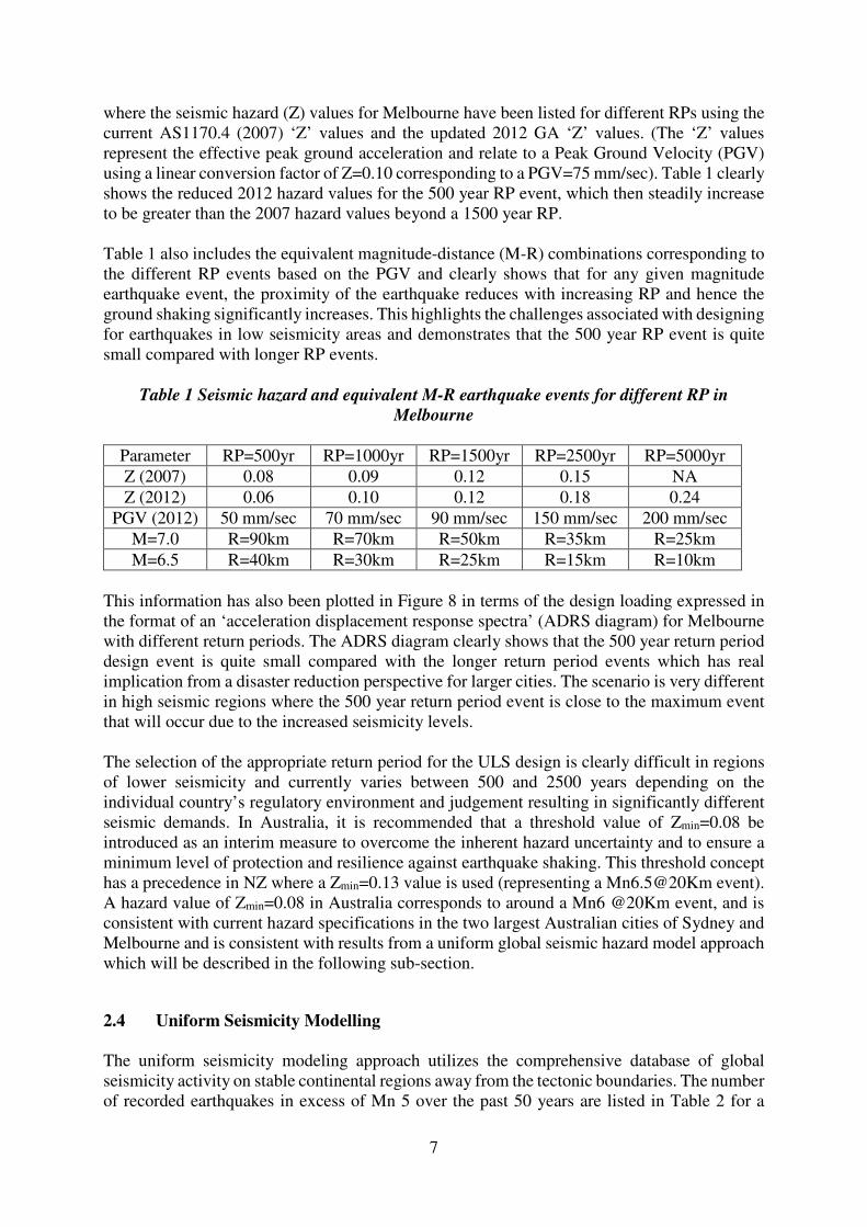
7

where the seismic hazard (Z) values for Melbourne have been listed for different RPs using the

current AS1170.4 (2007) ‘Z’ values and the updated 2012 GA ‘Z’ values. (The ‘Z’ values

represent the effective peak ground acceleration and relate to a Peak Ground Velocity (PGV)

using a linear conversion factor of Z=0.10 corresponding to a PGV=75 mm/sec). Table 1 clearly

shows the reduced 2012 hazard values for the 500 year RP event, which then steadily increase

to be greater than the 2007 hazard values beyond a 1500 year RP.

Table 1 also includes the equivalent magnitude-distance (M-R) combinations corresponding to

the different RP events based on the PGV and clearly shows that for any given magnitude

earthquake event, the proximity of the earthquake reduces with increasing RP and hence the

ground shaking significantly increases. This highlights the challenges associated with designing

for earthquakes in low seismicity areas and demonstrates that the 500 year RP event is quite

small compared with longer RP events.

Table 1 Seismic hazard and equivalent M-R earthquake events for different RP in

Melbourne

Parameter RP=500yr RP=1000yr RP=1500yr RP=2500yr RP=5000yr

Z (2007) 0.08 0.09 0.12 0.15 NA

Z (2012) 0.06 0.10 0.12 0.18 0.24

PGV (2012) 50 mm/sec 70 mm/sec 90 mm/sec 150 mm/sec 200 mm/sec

M=7.0 R=90km R=70km R=50km R=35km R=25km

M=6.5 R=40km R=30km R=25km R=15km R=10km

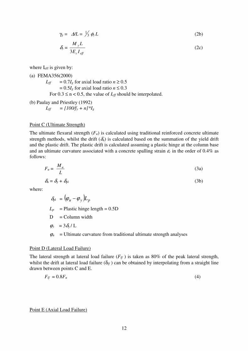
This information has also been plotted in Figure 8 in terms of the design loading expressed in

the format of an ‘acceleration displacement response spectra’ (ADRS diagram) for Melbourne

with different return periods. The ADRS diagram clearly shows that the 500 year return period

design event is quite small compared with the longer return period events which has real

implication from a disaster reduction perspective for larger cities. The scenario is very different

in high seismic regions where the 500 year return period event is close to the maximum event

that will occur due to the increased seismicity levels.

The selection of the appropriate return period for the ULS design is clearly difficult in regions

of lower seismicity and currently varies between 500 and 2500 years depending on the

individual country’s regulatory environment and judgement resulting in significantly different

seismic demands. In Australia, it is recommended that a threshold value of Zmin=0.08 be

introduced as an interim measure to overcome the inherent hazard uncertainty and to ensure a

minimum level of protection and resilience against earthquake shaking. This threshold concept

has a precedence in NZ where a Zmin=0.13 value is used (representing a Mn6.5@20Km event).

A hazard value of Zmin=0.08 in Australia corresponds to around a Mn6 @20Km event, and is

consistent with current hazard specifications in the two largest Australian cities of Sydney and

Melbourne and is consistent with results from a uniform global seismic hazard model approach

which will be described in the following sub-section.

2.4 Uniform Seismicity Modelling

The uniform seismicity modeling approach utilizes the comprehensive database of global

seismicity activity on stable continental regions away from the tectonic boundaries. The number

of recorded earthquakes in excess of Mn 5 over the past 50 years are listed in Table 2 for a

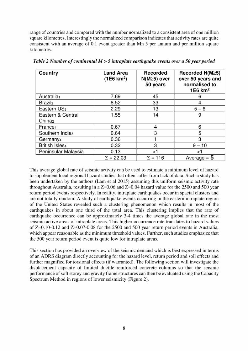
8

range of countries and compared with the number normalized to a consistent area of one million

square kilometres. Interestingly the normalized comparison indicates that activity rates are quite

consistent with an average of 0.1 event greater than Mn 5 per annum and per million square

kilometres.

Table 2 Number of continental M > 5 intraplate earthquake events over a 50 year period

Country Land Area (1E6 km2)

Recorded N(M≥5) over

50 years

Recorded N(M≥5) over 50 years and

normalised to 1E6 km2

Australia1 7.69 45 6

Brazil2 8.52 33 4

Eastern US3 2.29 13 5 − 6

Eastern & Central China2

1.55 14 9

France4 0.67 4 6

Southern India5 0.64 3 5

Germany4 0.36 1 3

British Isles4 0.32 3 9 − 10

Peninsular Malaysia 0.13 <1 <1

Σ = 22.03 Σ = 116 Average = 5

This average global rate of seismic activity can be used to estimate a minimum level of hazard

to supplement local regional hazard studies that often suffer from lack of data. Such a study has

been undertaken by the authors (Lam et al 2015) assuming this uniform seismic activity rate

throughout Australia, resulting in a Z=0.06 and Z=0.04 hazard value for the 2500 and 500 year

return period events respectively. In reality, intraplate earthquakes occur in spacial clusters and

are not totally random. A study of earthquake events occurring in the eastern intraplate region

of the United States revealed such a clustering phenomenon which results in most of the

earthquakes in about one third of the total area. This clustering implies that the rate of

earthquake occurrence can be approximately 3-4 times the average global rate in the most

seismic active areas of intraplate areas. This higher occurrence rate translates to hazard values

of Z=0.10-0.12 and Z=0.07-0.08 for the 2500 and 500 year return period events in Australia,

which appear reasonable as the minimum threshold values. Further, such studies emphasize that

the 500 year return period event is quite low for intraplate areas.

This section has provided an overview of the seismic demand which is best expressed in terms

of an ADRS diagram directly accounting for the hazard level, return period and soil effects and

further magnified for torsional effects (if warranted). The following section will investigate the

displacement capacity of limited ductile reinforced concrete columns so that the seismic

performance of soft storey and gravity frame structures can then be evaluated using the Capacity

Spectrum Method in regions of lower seismicity (Figure 2).

9

Figure 5 2012 GA Seismic hazard map for Australia (RP=500 years)

Figure 6 Current AS1170.4 Seismic hazard map for Australia (RP=500 years)

Figure 7 2012 GA Seismic hazard versus return period

10

Figure 8 ADRS diagram for a shallow soil site and different return periods

3. Drift Behaviour of Lightly Reinforced Concrete Columns

3.1 Background

In general, designers have a very good understanding of the strength characteristics of R/C

columns but very little understanding of the corresponding drift behaviour. This section

presents both a detailed and simplified push-over curve for lightly reinforced concrete columns

that can used to assess the seismic performance of soft storey structures. A parametric study

has also been undertaken to illustrate the drift behaviour and compare the two models.

The lateral load-drift behaviour and the maximum drift capacity of reinforced concrete columns

are directly affected by the following four design parameters: axial load ratio, longitudinal

reinforcement ratio, transverse reinforcement ratio and the aspect ratio:

• Axial load ratio: increases the flexural strength and significantly reduces drift capacity.

The higher the axial load ratio, the smaller the axial failure drifts particularly as the axial

load approaches or exceeds the balance point on the interaction diagram (Lynn et al

1996, Sezen et al 2004, Wibowo et al 2014a).

• Longitudinal reinforcement ratio: increases the flexural strength and decreases the drift

capacity. An increase in longitudinal reinforcement ratio tends to decrease the axial

failure drift, particularly for low axial load ratios. The effect reduces as the axial load

was increased towards the balance point of the column interaction diagram (Lynn et al

1996).

• Transverse reinforcement ratio: increases the lateral drift capacity without necessarily

increasing the flexural strength. The rate of increase in the axial load failure drift

capacity varies with some inter-dependency with the other design parameters (Priestley

et al 1996, 2007).

• Aspect ratio: affects the collapse behaviour and shifts the failure mode from a shear

mode to a flexural mode, but interestingly does not have a significant effect on the drift

capacity at axial load failure (Ousalem et al 2004, Wilson et al 2009).

Two lateral load-drift flexural models are presented in this section consisting of a detailed

column model and a simplified column model. The drift relationships are directly applicable to

0.000

0.100

0.200

0.300

0.400

0.500

0.600

0.700

0.800

0.900

1.000

0.00 0.02 0.04 0.06 0.08 0.10 0.12

Displacement (m)

Acc

ele

rati

on

(g

's)

5001000

1500

2500

5000

ADRS Diagram for Z=0.08

11

soft storey structures and multi storey buildings where the lateral drift maybe distributed over

many storeys.

3.2 Detailed Column Model

A push-over backbone curve model for predicting the lateral load-drift behaviour of reinforced

concrete columns is shown conceptually in Figure 9 in terms of cracking, yield, ultimate

strength, lateral load failure (80% peak) and axial load failure drift. This model is based on an

extensive database of past research and further details are provided in Wibowo et al (2014b).

Figure 9 Detailed column load-drift model

Point A (Cracking Strength)

The cracked lateral strength (Fcr) and corresponding drift (δcr) can be calculated from basic

mechanics as follows:

Fcr = L

M cr (1a)

δcr = gc

cr

IE

LM

3 (1b)

where the flexural tensile strength ft is taken as cf '6.0 consistent with most codes of

practice (such as AS3600), L is the effective cantilever length of the column, Ec is the

Young’s Modulus of concrete and Ig is the gross moment of inertia of the column cross-

section. The drift at cracking is typically in the order of 0.10%.

Point B (Yield Strength)

The yield strength (Fy) is calculated using classical yield moment (working stress) methods,

or approximated by the factored ultimate strength (assume φ=0.8). The yield drift (δy) is

calculated using classical curvature methods (equation 2b) or simply using the elastic drift

approach (equation 2c) and an effective second moment of area as described in FEMA356

(2000) or Paulay and Priestley (1992):

Fy = L

M y (2a)

12

γy = ∆/L = φy L (2b)

δy = effc

y

IE

LM

3 (2c)

where Ieff is given by:

(a) FEMA356(2000)

Ieff = 0.7Ig for axial load ratio n ≥ 0.5

= 0.5Ig for axial load ratio n ≤ 0.3

For 0.3 ≤ n < 0.5, the value of Ieff should be interpolated.

(b) Paulay and Priestley (1992)

Ieff = [100/fy + n]*Ig

Point C (Ultimate Strength)

The ultimate flexural strength (Fu) is calculated using traditional reinforced concrete ultimate

strength methods, whilst the drift (δu) is calculated based on the summation of the yield drift

and the plastic drift. The plastic drift is calculated assuming a plastic hinge at the column base

and an ultimate curvature associated with a concrete spalling strain εc in the order of 0.4% as

follows:

Fu = L

M u (3a)

δu = δy + δpl (3b)

where:

δpl = ( ) pyu Lϕϕ −

Lp = Plastic hinge length = 0.5D

D = Column width

ϕy = 3δy / L

ϕu = Ultimate curvature from traditional ultimate strength analyses

Point D (Lateral Load Failure)

The lateral strength at lateral load failure (Flf ) is taken as 80% of the peak lateral strength,

whilst the drift at lateral load failure (δlf ) can be obtained by interpolating from a straight line

drawn between points C and E.

Flf = 0.8Fu (4)

Point E (Axial Load Failure)

31

13

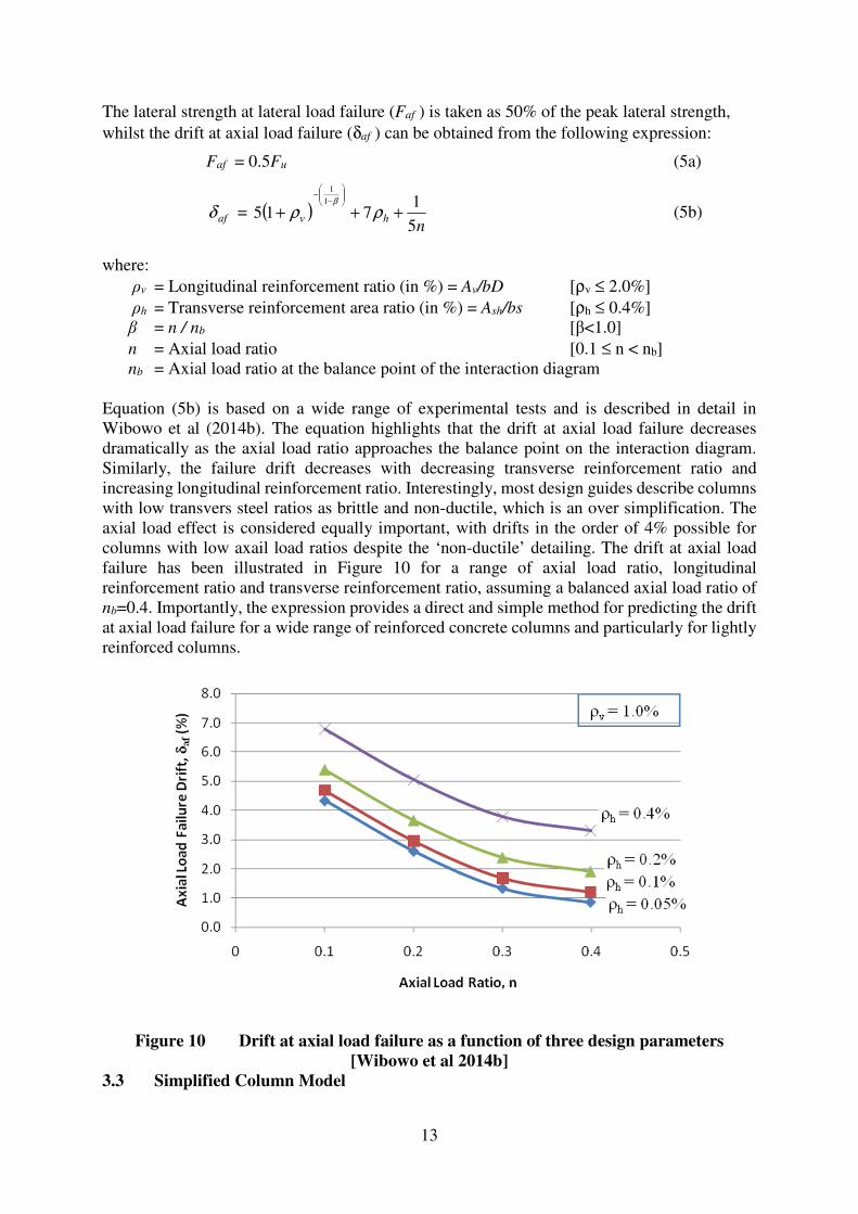
The lateral strength at lateral load failure (Faf ) is taken as 50% of the peak lateral strength,

whilst the drift at axial load failure (δaf ) can be obtained from the following expression:

Faf = 0.5Fu (5a)

afδ = ( )n

hv5

1715

1

1

+++

−−

ρρβ

(5b)

where:

ρv = Longitudinal reinforcement ratio (in %) = Av/bD [ρv ≤ 2.0%]

ρh = Transverse reinforcement area ratio (in %) = Ash/bs [ρh ≤ 0.4%]

β = n / nb [β<1.0]

n = Axial load ratio [0.1 ≤ n < nb]

nb = Axial load ratio at the balance point of the interaction diagram

Equation (5b) is based on a wide range of experimental tests and is described in detail in

Wibowo et al (2014b). The equation highlights that the drift at axial load failure decreases

dramatically as the axial load ratio approaches the balance point on the interaction diagram.

Similarly, the failure drift decreases with decreasing transverse reinforcement ratio and

increasing longitudinal reinforcement ratio. Interestingly, most design guides describe columns

with low transvers steel ratios as brittle and non-ductile, which is an over simplification. The

axial load effect is considered equally important, with drifts in the order of 4% possible for

columns with low axail load ratios despite the ‘non-ductile’ detailing. The drift at axial load

failure has been illustrated in Figure 10 for a range of axial load ratio, longitudinal

reinforcement ratio and transverse reinforcement ratio, assuming a balanced axial load ratio of

nb=0.4. Importantly, the expression provides a direct and simple method for predicting the drift

at axial load failure for a wide range of reinforced concrete columns and particularly for lightly

reinforced columns.

Figure 10 Drift at axial load failure as a function of three design parameters

[Wibowo et al 2014b]

3.3 Simplified Column Model

14

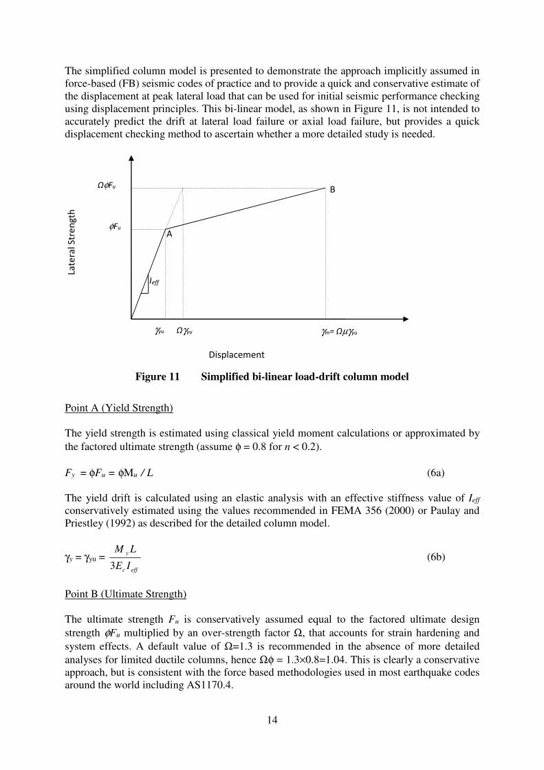
The simplified column model is presented to demonstrate the approach implicitly assumed in

force-based (FB) seismic codes of practice and to provide a quick and conservative estimate of

the displacement at peak lateral load that can be used for initial seismic performance checking

using displacement principles. This bi-linear model, as shown in Figure 11, is not intended to

accurately predict the drift at lateral load failure or axial load failure, but provides a quick

displacement checking method to ascertain whether a more detailed study is needed.

Figure 11 Simplified bi-linear load-drift column model

Point A (Yield Strength)

The yield strength is estimated using classical yield moment calculations or approximated by

the factored ultimate strength (assume φ = 0.8 for n < 0.2).

Fy = φFu = φMu / L (6a)

The yield drift is calculated using an elastic analysis with an effective stiffness value of Ieff

conservatively estimated using the values recommended in FEMA 356 (2000) or Paulay and

Priestley (1992) as described for the detailed column model.

γy = γyu = effc

y

IE

LM

3 (6b)

Point B (Ultimate Strength)

The ultimate strength Fu is conservatively assumed equal to the factored ultimate design

strength φFu multiplied by an over-strength factor Ω, that accounts for strain hardening and

system effects. A default value of Ω=1.3 is recommended in the absence of more detailed

analyses for limited ductile columns, hence Ωφ = 1.3×0.8=1.04. This is clearly a conservative

approach, but is consistent with the force based methodologies used in most earthquake codes

around the world including AS1170.4.

Displacement

γyu γm= Ωµγyu

φFu

ΩφFu

Late

ral S

tre

ng

th

A

B

Ieff

Ωγyu

15

Fu = ΩφFu (7a)

The ultimate drift (γm) is estimated as the product of the yield drift (γy), over-strength factor

(Ω=1.3) and representative system ductility factor (µ=2.0 for limited ductile systems) resulting

in the following expression:

γm = Ω µ γy = 2.6γy (7b)

3.4 Comparison of the Detailed and Simplified Column Models

The detailed column model provides a very good estimate of actual column lateral load-drift

behaviour as described in Wibowo et al [2014b]. Both the detailed and simplified column

models are compared using a case study example in this section involving a 500×500mm

cantilever column with an aspect ratio of a=4 and a variable axial load ratio in the range n=0.1

to n=0.5. All columns were reinforced with 6N24 Grade 500 corresponding to a longitudinal

reinforcing ratio of ρv =1.1% and a balance point on the interaction diagram corresponding to

an axial load ratio of nb=0.4. In all cases, R10 stirrups were used at 300mm spacing resulting

in a very low transverse reinforcement area ratio of ρh=0.1%.

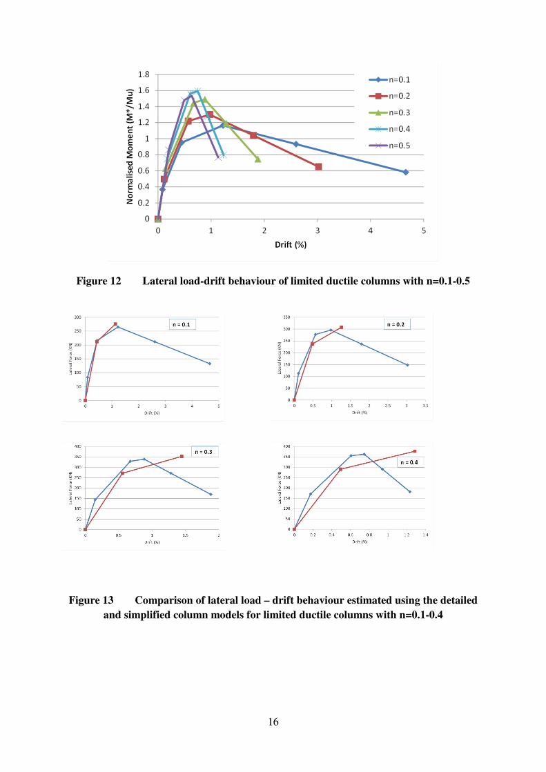
The detailed column model was used to estimate the five stages in the lateral load-drift

relationship (cracking, yield, ultimate strength, lateral load failure and axial load failure) for all

cases as shown in Figure 12. The axial load failure drift decreased significantly from 4.7% to

1.2% by increasing the axial load ratio from n=0.1 to n=0.5. This significant decrease in drift

capacity is clearly associated with the much steeper strength degradation post peak with

increasing axial load in limited ductile columns.

The simplified model provides a reasonable and conservative estimate of the drift at peak lateral

load using code strength values as shown in Figure 13, in which the bilinear model results are

compared with the detailed backbone curve for the case study example. The results indicate that

the use of a constant ductility factor based on the level of detailing and independent of the level

of axial load provides a conservative maximum displacement prediction, particularly for

columns with low axial load ratios (ie. compare n=0.1 with n=0.4). The simplified bi-linear

model allows a designer to undertake a quick and conservative check on the seismic

performance of column elements using displacement based principles. Further practical design

guidelines for estimating the load-deflection behaviour of limited ductile columns and structural

walls are presented in Wilson et al (2015).

16

Figure 12 Lateral load-drift behaviour of limited ductile columns with n=0.1-0.5

Figure 13 Comparison of lateral load – drift behaviour estimated using the detailed

and simplified column models for limited ductile columns with n=0.1-0.4

17

3.5 Displacement Capacity Curves

The lateral load drift column models can be converted into an equivalent SDOF capacity curve

in an acceleration displacement format for a soft storey structure using the following simple

relationship:

Acceleration = F / M (8a)

Displacement = δ . h (8b)

where, F is the lateral force, M is the building mass, δ is the associated drift and h is the soft

storey height.

The capacity curve can be superimposed on the seismic demand curve to evaluate the seismic

performance of the soft storey building as shown in Figure 2. Alternatively, the performance of

the building can be assessed using a ‘first tier’ approach by comparing the peak displacement

demand (PDD) with the displacement capacity (∆c) of the soft storey. The structure is deemed

satisfactory (in terms of its performance against the specified return period event) if PDD is

less than ∆c. The displacement capacity of a soft storey building with lightly reinforced concrete

columns ranges from ∆c 40mm to 200mm, assuming a soft storey height of 4.0m and a drift

capacityδc range of 1.0% to 5.0% depending on the axial load load ratio (refer Figure 10).

4. Conclusion

Soft storey buildings are common in regions of lower seismicity and are considered to be

particulalry vulnerable to earthquake excitation due to the limited energy absorption and

displacement capacity of the limited ductile columns that not only have to support the weight

of the building but also to undergo significant drift. This paper has presented a displacement

based (DB) method for assessing the seismic performance of reinforced concrete framed

buildings and particularly soft storey buildings. The DB method presented addresses both the

challenges of defining appropriate hazaed levels in lower seismicity regions and developing

representative load-drift curves for limited ductile concrete structures.

The peak displacement demands in regions of lower seismicity are typically in the range of

PDD=20-100mm depending on the soil conditions for a 500 year return period event. These

displacement demands can be magnified further due to torsional response effects and longer

return period events. The appropriateness of using a probabilistic hazard analysis to assess the

seismic hazard in regions of lower seismicity has shortcomings given the paucity of data and

that the maximum considered earthquake may have a return period in the order of 5,000 to

10,000 years. It is recommended that a minimum threshold hazard value of Z=0.08 be

introduced in the Australian Earthquake Loading Standard as an interim measure to address

some of the inherent uncertainties of the PHSA method when applied to regions with a lack of

data.

A detailed column model for predicting the lateral load-drift behaviour of reinforced concrete

columns based on an extensive database of past research has been described comprising five

stages; cracking, yield, ultimate strength, lateral load failure and axial load failure. Importantly,

the model predicts the drift at axial load failure in terms of three design parameters; axial load

ratio, longitudinal reinforcement ratio and transverse reinforcement ratio.

In general, designers have a very good understanding of the strength characteristic of reinforced

concrete columns and structural walls but have limited understanding of the corresponding drift

18

behaviour which is essential for assessing the earthquake performance of such structures using

displacement based principles. To address this issue, this paper has presented a detailed and

simplified model for estimating the load-drift behaviour of both reinforced concrete columns

and structural walls.

The simplified column and wall models have been constructed based on the assumption

underlying most force based seismic codes of practice, where the inelastic behaviour is

represented by a ductility factor µ and over-strength factor Ω. The simplified bi-linear column

and wall models provide a reasonable and conservative load-deflection plot up to the peak

lateral load. This simplified curve is useful for undertaking a quick and conservative check on

the seismic performance of critical columns using displacement principles and the capacity

spectrum method.

The detailed push-over curve of a lightly reinforced concrete column was calculated for axial

load ratios varying from n=0.1-0.5 and clearly demonstrated the significant effect axial load

has on reducing the drift capacity. The displacement capacity of a soft storey building ranges

from 40mm to 200mm assuming a soft storey height of 4.0m. This reflects a drift capacity range

of 1.0% to 5.0% for lightly reinforced concrete columns and is very dependent on the axial load

ratio despite the ‘non-ductile’ detailing. Clearly, designers can increase the drift capacity of

their structures by increasing the column size and reducing the axial load ratio to below the

balance point, in addition to increasing the transverse steel ratio.

5. Acknowledgements

The authors acknowledge the financial assistance provided by the Australian Research Council

with grants DP1096753 and DP0772088 investigating the drift performance of reinforced

concrete columns and structural walls.

6. References Applied Technology Council, 1996, ‘ATC-40: Seismic evaluation and retrofit of concrete buildings 1&2’,

California, USA.

AS3600-2011, ‘Concrete Structures’, Standards Australia.

AS1170.4-2007, ‘Structural design actions, Part 4: Earthquake Actions in Australia’, Standards Australia.

FEMA273, 1997, ‘NEHRP Guideline for the Seismic Rehabilitation of Buildings’, Washington DC, Federal

Emergency Management Agency, USA.

FEMA 356, 2000, ‘NEHRP Guidelines for the seismic rehabilitation of buildings’, Federal Emergency

Management Agency, Washington DC, USA.

Lam NTK, Wilson JL, Hutchinson GL, 1996, ‘Review of torsional coupling of asymmetrical wall-frame

building’, Journal of Engineering Structures, Vol 19, pp 233-246.

Lam, NTK., Wilson JL, Chandler AM, 2001, ‘Seismic displacement response spectrum estimated from the

frame analogy soil amplification model’, Journal of Engineering Structures, Vol 23 pp 1437-1452.

Lam NTK, Sinadinovski C, Koo R, Wilson JL, 2003, ‘Peak ground velocity modelling for Australian

Intraplate earthquakes’, International Journal of Seismology and Earthquake Engineering, Vol 5(2) pp

11-22.

Lam NTK, Wilson JL, 2004, ‘Displacement modelling of Intraplate earthquakes’, International Seismology

and Earthquake Technology Journal (special issue on Performance Based Seismic Design; Ed Nigel

Priestley), Indian Institute. of Technology, Vol 41(1), paper no. 439, pp 15-52.

Lam NTK, Wilson JL, Hutchinson GL, 2000a, ‘Generation of synthetic earthquake accelerograms using

seismological modelling: a review’, Journal of Earthquake Engineering, Vol 4(3): 321-354.

19

Lam NTK, Wilson JL, Chandler AM, Hutchinson GL, 2000b, ‘Response Spectral Relationships for Rock

Sites Derived from the Component Attenuation Model’, Earthquake Engineering and Structural

Dynamics, Vol 29(10): 1457-1490.

Lam NTK, Wilson JL, Chandler AM, Hutchinson GL, 2000c, ‘Response Spectrum Modelling for Rock Sites

in Low and Moderate Seismicity Regions Combining Velocity, Displacement and Acceleration

Predictions’, Earthquake Engineering and Structural Dynamics, Vol 29(10):1491-1526.

Lam NTK, Chandler AM, 2005, ‘Peak Displacement Demand in Stable Continental Regions’, Earthquake

Engineering and Structural Dynamics ,Vol 34: 1047-1072.

Lam NTK, Tsang HH, Lumantarna E, Wilson JL, 2015, ‘Results of probabilistic seismic hazard analysis

assuming uniform distribution of seismicity’, Pacific Conference on Earthquake Engineering, 10th PCEE

Proceedings, Sydney, Australia, Nov 6-8.

Leonard M, Burbridge D, Edwards M, 2013, ‘Atlas of seismic hazard maps of Australia’, Geoscience

Austtalia, Record 2013/41, Australian Government, 39pp.

Lumantarna E, Wilson JL, Lam NTK, 2012, ‘Bi-linear Displacement Response Spectrum Model for

Engineering Applications in Low and Moderate Seismicity Regions’, Journal of Soil Dynamics and

Earthquake Engineering, Vol 43, pp 85-96.

Lumantarna E, Lam NTK, Wilson JL, 2013, ‘Displacement controlled behaviour of asymmetrical single

storey buildings’, Journal of Earthquake Engineering, Vol 17 pp 902-917.

Lynn AC, Moehle JP, Mahin SA and Holmes WT, 1996, ‘Seismic evaluation of existing reinforced concrete

columns’, Earthquake Spectra, Earthquake Engineering Research Institute, Vol 12, No 4, pp 715-739.

Mander JB, Priestley MJN, Park R, 1988, ‘Theoretical stress-strain model for concrete’, ASCE Journal

Structural Division, Vol 119(8): 1804-1826.

Ousalem H, Kabeyasawa T, Tasai A, 2004, ‘Evaluation of ultimate deformation capacity at axial load

collapse of reinforced concrete columns’, Thirteenth World Conference on Earthquake Engineering,

Vancouver, British Columbia, Canada, Paper No 370.

Park R, Paulay T, 1975, ‘Reinforced Concrete Structures’, John Wiley & Sons, New York, 769 pp.

Park R, 1997, ‘A static force-based procedure for the seismic assessment of existing reinforced concrete

moment resisting frames’, Bulletin of The New Zealand National Society for Earthquake Engineering,

Vol 30(3): 213-226.

Paulay T, Priestley M, 1992, ‘Seismic design of reinforced concrete and masonry structures’, John Wiley

and Sons, New York, USA.

Priestley MJN, Calvi GM, Kowalsky MJ, 2007, ‘Displacement-Based Seismic Design of Structures’, IUSS

Press, Pavia, Italy, 721 pp.

Priestley MJN, Seible F, Calvi GM, 1996, ‘Seismic Design and Retrofit of Bridges’, John Wiley & Sons,

New York, USA.

Sezen H and Moehle JP, 2004, ‘Shear strength model for lightly reinforced concrete columns’, Journal of

Structural Engineering, ASCE, Vol. 130(11), pp 1692-1703.

Wibowo A, Wilson JL, Lam NTK, Gad EF, 2009, ‘Collapse modelling analysis of a precast soft-storey

building in Australia’, Journal of Engineering Structures, Vol 32, pp 1925-1936.

Wibowo A, Wilson JL, Lam NTK, Gad EF, 2014a, ‘Drift Capacity of Lightly Reinforced Concrete Columns’,

Australian Journal of Structural Engineering, Vol 15, No 2, pp 131-150.

Wibowo A, Wilson JL, Lam NTK, Gad EF, 2014b, ‘Drift performance of lightly reinforced concrete

columns’, Journal of Engineering Structures, Vol 59, pp 522-535.

Wilson JL, Lam NTK, Rodsin K, 2009, ‘Collapse Modelling of Soft Storey Buildings’. Australian Journal

of Structural Engineering, Vol 10 No 1, pp 11-23.

Wilson JL, Lam NTK, 2006, ‘Earthquake design of buildings in Australia by velocity and displacement

principles’, Australian Journal of Structural Engineering, Vol .6 No 2, pp 103-118.

Wilson JL, Wibowo A, Lam NTKL, Gad EF, 2015, “Drift behaviour of lightly reinforced concrete columns

and structural walls for design applications”, Australian Journal of Structural Engineering, Vol 16, No 1,

pp 62-73.