hbm2 - reference manual

HBM2 - Reference Manual

Copyright © August 27, 2018 Motek BV

SW011-7002-1.0

- 3 -

Preface

Motek provides innovative products for rehabilitation, orthopedics, neurology, performance

enhancements and research. Motion platforms, instrumented treadmills, motion-capture

systems and surround sound are combined with integrated Virtual Reality (VR) environments

to train movement functions and improve (dynamic) stability.

We hope you will enjoy using the HBM and that it helps you to improve clinical care.

Regards,

Motek

- 5 -

Contents

1. Introduction......................................................................................................................- 7 -

Changes in the 2017 update ...........................................................................................- 7 -

2. Marker set........................................................................................................................- 9 -

3. Model Initialization.........................................................................................................- 12 -

3.1 Static Initialization .......................................................................................................- 12 -

3.2 Functional hip joint calibration ....................................................................................- 13 -

3.3 Functional knee joint calibration .................................................................................- 13 -

4. Skeleton Model..............................................................................................................- 14 -

4.1 Foot .............................................................................................................................- 15 -

4.2 Shank ..........................................................................................................................- 16 -

4.3 Thigh ...........................................................................................................................- 17 -

4.4 Pelvis ..........................................................................................................................- 18 -

4.5 Trunk ...........................................................................................................................- 18 -

4.6 Upper arm ...................................................................................................................- 19 -

4.7 Forearm ......................................................................................................................- 20 -

4.8 Hand ...........................................................................................................................- 20 -

4.9 Head ...........................................................................................................................- 20 -

4.10 Mass properties ........................................................................................................- 22 -

5. Biomechanical Analysis ................................................................................................- 23 -

5.1 Kinematics ..................................................................................................................- 23 -

Kinematic degrees of freedom ......................................................................................- 23 -

Inverse kinematics ........................................................................................................- 24 -

Filtering and differentiation............................................................................................- 25 -

5.2 Kinetics .......................................................................................................................- 25 -

Generalized forces ........................................................................................................- 25 -

Inverse dynamics ..........................................................................................................- 26 -

5.3 Muscle properties .......................................................................................................- 26 -

Muscle moment arms ....................................................................................................- 29 -

Muscle force estimation ................................................................................................- 29 -

6. References ....................................................................................................................- 31 -

- 7 -

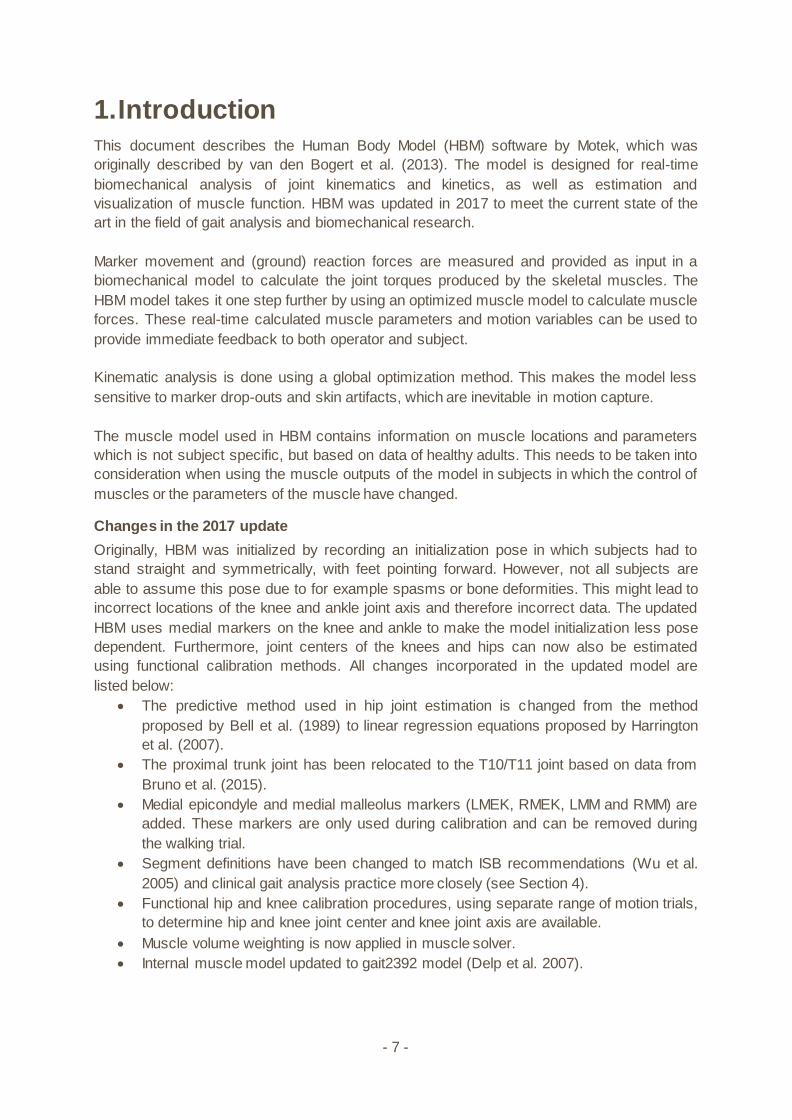
1. Introduction

This document describes the Human Body Model (HBM) software by Motek, which was

originally described by van den Bogert et al. (2013). The model is designed for real-time

biomechanical analysis of joint kinematics and kinetics, as well as estimation and

visualization of muscle function. HBM was updated in 2017 to meet the current state of the

art in the field of gait analysis and biomechanical research.

Marker movement and (ground) reaction forces are measured and provided as input in a

biomechanical model to calculate the joint torques produced by the skeletal muscles. The

HBM model takes it one step further by using an optimized muscle model to calculate muscle

forces. These real-time calculated muscle parameters and motion variables can be used to

provide immediate feedback to both operator and subject.

Kinematic analysis is done using a global optimization method. This makes the model less

sensitive to marker drop-outs and skin artifacts, which are inevitable in motion capture.

The muscle model used in HBM contains information on muscle locations and parameters

which is not subject specific, but based on data of healthy adults. This needs to be taken into

consideration when using the muscle outputs of the model in subjects in which the control of

muscles or the parameters of the muscle have changed.

Changes in the 2017 update

Originally, HBM was initialized by recording an initialization pose in which subjects had to

stand straight and symmetrically, with feet pointing forward. However, not all subjects are

able to assume this pose due to for example spasms or bone deformities. This might lead to

incorrect locations of the knee and ankle joint axis and therefore incorrect data. The updated

HBM uses medial markers on the knee and ankle to make the model initialization less pose

dependent. Furthermore, joint centers of the knees and hips can now also be estimated

using functional calibration methods. All changes incorporated in the updated model are

listed below:

• The predictive method used in hip joint estimation is changed from the method

proposed by Bell et al. (1989) to linear regression equations proposed by Harrington

et al. (2007).

• The proximal trunk joint has been relocated to the T10/T11 joint based on data from

Bruno et al. (2015).

• Medial epicondyle and medial malleolus markers (LMEK, RMEK, LMM and RMM) are

added. These markers are only used during calibration and can be removed during

the walking trial.

• Segment definitions have been changed to match ISB recommendations (Wu et al.

2005) and clinical gait analysis practice more closely (see Section 4).

• Functional hip and knee calibration procedures, using separate range of motion trials,

to determine hip and knee joint center and knee joint axis are available.

• Muscle volume weighting is now applied in muscle solver.

• Internal muscle model updated to gait2392 model (Delp et al. 2007).

- 8 -

Changes in marker set

• The BBAC marker is removed from the markerset

• LGTRO and RGTRO (greater trochanter) markers are removed to avoid soft tissue

artifacts associated with this marker.

• SACR (sacrum) and NAVE (navel) markers are removed as they are no longer

necessary for visualization, and to avoid soft tissue artifacts associated with these

markers.

• The TOE marker is moved from the tip of the big toe to the caput of the 2nd metatarsal

bone, and is now called MT2.

• Several marker names are changed. STRN marker is now called JN (jugular notch),

FLTHI/FRTHI changed to LLTHI/RLTHI, and LATI/RATI are now called

LLSHA/RLSHA.

• The placement of the thigh and shank markers has changed.

- 9 -

2. Marker set

The HBM uses a marker set containing 46 markers (Figure 1, Table 1) to create a skeleton

model and to solve skeleton motion. Each marker is assigned to a certain body segment and

has its own weighting for the appropriate segment.

The bold markers in Table 1 and green markers in Figure 1 are anatomical markers needed

to define the joint centers and segments of the model during initialization. These markers

need to be placed accurately in order to get reliable results. The other markers are technical

markers providing redundancy and robustness for the model. Therefore, placement of these

markers is less critical. They are also used for the functional calibration of the knee and hip.

Note that the medial markers on the knee and ankle (LMEK, LMM, RMEK, and RMM) can be

removed after model initialization since these are only used during initialization to determine

joint centers and segment reference frames. This feature was added because these markers

often tend to detach during gait.

Figure 1. Front, side, and rear view of the marker set used in the Human Body Model. Green markers are anatomical markers

used to define the skeleton during initialization.

*These markers are optional. If used, they may be removed after model initialization.

- 10 -

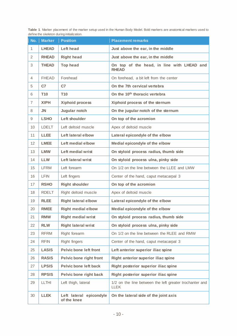
Table 1. Marker placement of the marker setup used in the Human Body Model. Bold markers are anatomical markers used to

define the skeleton during initialization.

No. Marker Position Placement remarks

1 LHEAD Left head Just above the ear, in the middle

2 RHEAD Right head Just above the ear, in the middle

3 THEAD Top head On top of the head, in line with LHEAD and RHEAD

4 FHEAD Forehead On forehead, a bit left from the center

5 C7 C7 On the 7th cervical vertebra

6 T10 T10 On the 10th thoracic vertebra

7 XIPH Xiphoid process Xiphoid process of the sternum

8 JN Jugular notch On the jugular notch of the sternum

9 LSHO Left shoulder On top of the acromion

10 LDELT Left deltoid muscle Apex of deltoid muscle

11 LLEE Left lateral elbow Lateral epicondyle of the elbow

12 LMEE Left medial elbow Medial epicondyle of the elbow

13 LMW Left medial wrist On styloid process radius, thumb side

14 LLW Left lateral wrist On styloid process ulna, pinky side

15 LFRM Left forearm On 1/2 on the line between the LLEE and LMW

16 LFIN Left fingers Center of the hand, caput metacarpal 3

17 RSHO Right shoulder On top of the acromion

18 RDELT Right deltoid muscle Apex of deltoid muscle

19 RLEE Right lateral elbow Lateral epicondyle of the elbow

20 RMEE Right medial elbow Medial epicondyle of the elbow

21 RMW Right medial wrist On styloid process radius, thumb side

22 RLW Right lateral wrist On styloid process ulna, pinky side

23 RFRM Right forearm On 1/2 on the line between the RLEE and RMW

24 RFIN Right fingers Center of the hand, caput metacarpal 3

25 LASIS Pelvic bone left front Left anterior superior iliac spine

26 RASIS Pelvic bone right front Right anterior superior iliac spine

27 LPSIS Pelvic bone left back Right posterior superior iliac spine

28 RPSIS Pelvic bone right back Right posterior superior iliac spine

29 LLTHI Left thigh, lateral 1/2 on the line between the left greater trochanter and LLEK

30 LLEK Left lateral epicondyle of the knee

On the lateral side of the joint axis

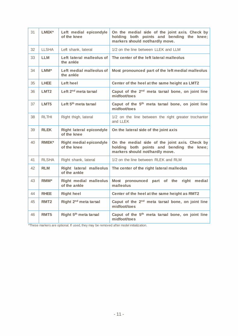
- 11 -

31 LMEK* Left medial epicondyle of the knee

On the medial side of the joint axis. Check by holding both points and bending the knee; markers should not/hardly move.

32 LLSHA Left shank, lateral 1/2 on the line between LLEK and LLM

33 LLM Left lateral malleolus of the ankle

The center of the left lateral malleolus

34 LMM* Left medial malleolus of the ankle

Most pronounced part of the left medial malleolus

35 LHEE Left heel Center of the heel at the same height as LMT2

36 LMT2 Left 2nd meta tarsal Caput of the 2nd meta tarsal bone, on joint line midfoot/toes

37 LMT5 Left 5th meta tarsal Caput of the 5th meta tarsal bone, on joint line

midfoot/toes

38 RLTHI Right thigh, lateral 1/2 on the line between the right greater trochanter and LLEK

39 RLEK Right lateral epicondyle of the knee

On the lateral side of the joint axis

40 RMEK* Right medial epicondyle

of the knee

On the medial side of the joint axis. Check by

holding both points and bending the knee; markers should not/hardly move.

41 RLSHA Right shank, lateral 1/2 on the line between RLEK and RLM

42 RLM Right lateral malleolus of the ankle

The center of the right lateral malleolus

43 RMM* Right medial malleolus

of the ankle

Most pronounced part of the right medial

malleolus

44 RHEE Right heel Center of the heel at the same height as RMT2

45 RMT2 Right 2nd meta tarsal Caput of the 2nd meta tarsal bone, on joint line

midfoot/toes

46 RMT5 Right 5th meta tarsal Caput of the 5th meta tarsal bone, on joint line midfoot/toes

*These markers are optional. If used, they may be removed after model initialization.

- 12 -

3. Model Initialization

Static initialization of the model is done by recording an initialization pose. Optionally,

functional hip and knee joint calibrations can be performed. The functional calibrations have

to be performed before the static calibration, to be incorporated in the model. When the static

calibration is done prior to the functional calibration, the functional calibration will remain

unused until a new static calibration is performed.

For most patients, static model calibration is preferred as functional joint calibration requires

the subject to perform complex calibration motions with extensive ranges of motion in both

the hip as well as the knee. Recent research also suggests that locating the hip joint center

using the Harrington equations generally works as well as, or better than, functional

calibration (Peters et al. 2012; Sangeux et al. 2011; Sangeux et al. 2014).

3.1 Static Initialization

The static calibration can be done with or without the use of medial knee and ankle markers.

In earlier versions of HBM, these medial markers were not included in the marker set. Using

the medial markers makes the initialization less pose dependent, which will especially be

helpful with subjects who are not able to assume the initialization pose. The calibration

without medial markers is still available.

During initialization the position of joint centers, bone lengths, and joint axes are estimated

based on:

• Marker coordinates during initialization pose

• Marker diameter [m]

• Knee width [m] (when no medial markers are used)

• Ankle width [m] (when no medial markers are used)

To estimate mass properties of the body segments, the following additional information is

needed:

• Subject weight [kg]

• Subject gender

To perform the static initialization, the subject is placed in an initialization pose. The exact

execution of the pose is essential when no medial markers are used, since the calibration will

be pose dependent in that case. However, even when medial markers are used try to meet

the following guidelines as well as possible:

• The subject should stand upright, looking forward, arms about 45 degrees

abducted. The direction the subject is facing is not important, since the software

automatically compensates for this direction.

• Feet should be pointing forward, approximately at hip width. This can be

confirmed by doing knee bends in which the distance between the knees should

remain constant.

• Arms and legs must be straight (neutral flexion-extension angle), with palms of the

hand facing downwards.

- 13 -

3.2 Functional hip joint calibration

A functional hip joint calibration can be performed to determine the joint center of the hip.

Subjects should start by standing upright, thereafter; the subject has to perform a star arc

movement, which was found to be the movement which leads to the most accurate results

according to Camomilla et al. (2006). The star arc movement described in Camomilla et al.

(2006) is slightly adapted since excessive hip extension causes significant skin movement

artifacts. The adapted star arc consists of five different movements as described below

(Figure 2):

1. Hip flexion, then back to neutral.

2. Combination of hip flexion and abduction, then back to neutral.

3. Hip abduction, then back to neutral.

4. Combination of hip extension and abduction, then back to neutral.

5. A full circumduction movement is made with the hip.

Figure 2. Transverse view of the f ive movements of the star arc for the calibration of the right hip.

To create as little as possible soft tissue movement in the thigh, subjects should be asked to

avoid internal and external rotation of the hip and to minimize frontal rotation of the pelvis

(Leardini et al. 1999). Please note that the star motion has to be performed for each leg

individually. To use the functional hip calibration, HBM requires a minimal range of motion of

60 degrees of flexion/extension and 30 degrees of abduction (Kainz et al. 2015).

3.3 Functional knee joint calibration

Similar to the functional hip joint calibration, subjects should start by standing upright.

Subjects should flex and extend the knee about five times through a range of approximately

0 to 90° of flexion. This calibration also needs to be done for each leg individually.

- 14 -

4. Skeleton Model

The skeleton model is designed for real-time biomechanical analysis of the human body, and

involves all kinematic degrees of freedom (DOF) which are controlled by muscles. The trunk

is modeled as two segments which are coupled to give three degrees of freedom. Figure 3

shows the 18-segment skeleton model, which has a total of 46 DOF.

Figure 3. Hierarchy of the skeleton model: The pelvis is the root segment, w hich has six degrees of freedom (DOF) relative to

the w orld. Numbers besides the segments represent the DOF added by that segment. The tw o DOFs of ankle and subtalar joint

are combined in this diagram. The total number of DOF of the skeleton model is 46.

HBM generates the following list of body segment names:

• Pelvis

• Abdomen

• Thorax

• Head

• RUpperArm

• LUpperArm

• RForeArm

• LForeArm

• RHand

• LHand

• RFemur

• LFemur

• RShank

• LShank

• RFoot

• LFoot

• RToe

• LToe

6

3

3

6 6

2

3 3

1 1

2 2

2

2 2

1 1

- 15 -

For each segment a reference frame is needed to define the equations of motion (Figure 4).

These segment reference frames are defined only once during model initialization.

Thereafter, the segments’ marker coordinates and joint centers are expressed as constants

relative to these reference frames. During motion, the markers and joints define skeleton

motion via the inverse kinematics as described in Section 5.1.

As a general principle, the origin of each segment is placed in the proximal joint (i.e. the

connection onto the parent bone), except for pelvis, which is the root of the hierarchy. As a

general rule, the segment Z-axis is defined to go through its distal joint (when available). This

is also consistent with de Leva (1996), so that the local X- and Y-coordinates of the center of

mass, for all segments, are zero. The segment Z-axis will generally point up when standing

upright. This means the centers of mass in the arm and leg segments have negative Z-

coordinates. The advantage of defining the Z-axis this way is that the model stands perfectly

straight when all rotations are zero (except in the ankles). Rotations are then easier to

interpret.

Joint axes are defined so that kinematic data are compatible with clinical definitions. These

are based on the ISB standards (Wu et al. 1995, 2002, 2005), unless when these are not

practical for clinical use.

Joint axes are also needed to constrain the motion of the model, so that the model

represents muscle function, and not the small motions (e.g. knee abduction and rotation, joint

translations) that are not controlled by muscles.

The remainder of this section describes the definitions of the segments and how these are

constructed during the model initialization. As the origin of each segment is placed in the

proximal joint, the segments are described bottom up starting with most distal joint (the foot)

working back up towards the parent segment and end with the trunk. For each segment the

construction of the proximal joint center is described first, as this will be the origin for the

segment reference frame (which is described second). Finally the joint axes and joint angles

are described.

4.1 Foot

Joint centers

Ankle joint

The ankle joint center is assumed to be the midpoint between the lateral and medial

malleolus. If both lateral and medial ankle markers are available, the ankle joint center is

defined as midpoint between these two markers. When no medial malleolus marker is used,

the ankle joint center will be defined as ‘half of ankle width + marker radius’ medial to the

lateral marker. Medial direction in this case is a horizontal projection of the vector from

RASIS to LASIS.

Subtalar joint

According to van den Bogert et al. (1994) the subtalar joint center is defined 12mm below the

ankle joint center. In HBM, this is implemented as a displacement along the X-axis of the

foot. This proposed 12mm was scaled by tibia length as follows:

- 16 -

Tibia length/0.375 ∗ 12

in which tibia length is the distance between lateral knee and ankle markers.

Reference frame

The origin of the foot is located in the subtalar joint center. The Z-axis is parallel to the vector

from MT2 to HEE markers (which should be horizontally when the foot is flat on the ground)

and points posteriorly. In this way HBM will report a 90° flexion angle when standing in

neutral pose. The X-axis is based on the Z-axis and a temporal Y-axis, for which two

possibilities exist, depending on the presence of the medial ankle marker. When a medial

marker is present, a temporal Y-axis between the lateral and medial malleolus pointing to the

left is defined. In case the medial marker is not present, the temporal Y-axis is parallel to the

line between the two ASIS markers and pointing to the left. The X-axis is the cross product of

the temporal Y-axis and the Z-axis, and will point dorsally. The Y-axis is the cross product of

the Z- and X-axis.

Joint axes and joint angles (degrees of freedom)

The ankle is modeled as two hinges, based on Isman’s normative data (Isman & Inman

1969; van den Bogert et al. 1994). Using three hinges would lead to overestimation of

muscle forces as in Burdett (1982), a problem nicely described by Glitsch & Baumann

(1997). Between the two joint axes a distance of 12 mm is assumed according to van den

Bogert et al. (1994) which is scaled in HBM by tibia length as mentioned above. A talus

segment is not explicitly defined, since its mass can be ignored and only has a kinematic

role. The ankle thus has two degrees of freedom, which are plantar flexion (rotation about the

Y-axis of the shank reference frame; plantar flexion is positive) and pronation/supination

(rotation about the pronation/supination axis; pronation is positive). The pronation/supination

axis is not aligned with the foot coordinate axes, but is defined in the foot reference frame

using the average subtalar joint (STJ) in Isman & Inman (1969) and points forward.

According to Isman and Inman, the STJ is inclined 42 degrees from the horizontal plane, and

deviates 23 degrees medially from the sagittal plane. Therefore, our STJ axis is for the right

foot:

𝑆𝑇𝐽 = [

cos(42°) cos (23°)

cos(42°) sin (23°)sin (42°)

]

4.2 Shank

Knee joint center

Three different methods can be used to determine the knee joint center. Two different

methods for static initialization are available, and one method is available for functional knee

calibration. The knee joint center is assumed to be the midpoint between the lateral and

medial epicondyle. If both lateral and medial knee markers are available during static

initialization, the knee joint center is defined as midpoint between these two markers. When

no medial knee marker is used, the knee joint center will be defined as ‘half of knee width +

marker radius’ medial to the lateral marker. Medial direction in this case is a horizontal

projection of the vector from RASIS to LASIS.

- 17 -

In case of functional knee calibration, knee axes are estimated using the axis of rotation

estimation method by Gamage & Lasenby (2002), as was recommended by van Campen et

al. (2011) and MacWilliams (2008). This method assumes that the markers on the shank

(LM, MM, and LSHA) rotate about a fixed axis of rotation relatively to the thigh. A least

squares cost function is used to find the best fitting axis. The knee joint center is defined as

the projection of the midpoint between the medial and lateral epicondyle onto this axis.

Reference frame

The origin of the shank is located in the knee joint center. The negative Z-axis points towards

the ankle joint center. A temporal Y-axis is constructed along the ankle axis and points to the

left (see section 4.1). The X-axis is the cross product of the Z-axis and the temporal Y-axis.

The Y-axis is the cross product of the Z- and X-axis to ensure orthonormality.


The knee is modeled as one hinge, since Glitsch & Baumann (1997) have shown that this is

best for the analysis of muscle function and estimation of muscle forces. Also, the

abduction/adduction range of motion is very small. As to internal/external rotation, the knee

does have a 45 degrees range of motion when flexed 90 degrees. During gait however, the

knee is extended so there will be little internal/external rotation. Therefore, modeling these

movements would most likely reflect inherent crosstalk errors in the 3D kinematic

calculations, rather than a true anatomical movement (Ramakrishnan & Kadaba 1991). Thus,

the knee has one degree of freedom, which is flexion/extension (rotation around the Y-axis;

flexion is positive). Ab/adduction and internal/external rotation angles are constant, set during

initialization.

4.3 Thigh

Hip joint center

A predictive method has to be used to determine the hip joint center (HJC) in case of the

static model initialization, while a functional approach is used in case of functional hip

calibration. Several studies comparing different methods of HJC estimation (Assi et al. 2016;

Kainz et al. 2016; Peters et al. 2012; Sangeux et al. 2011; Sangeux et al. 2014) showed that

the method of Harrington et al. (2007) is the most accurate predictive method.

The most accurate functional approach was found to be the geometric sphere fit method by

Gamage and Lasenby (2002) (Kainz et al. 2015; MacWilliams 2008; Sangeux et al. Baker

2011; Sangeux et al. 2014). Hence, these two methods are implemented in the HBM.

Harrington equations

The Harrington equations (Harrington et al. 2007) are linear regression equations to predict

the location of the HJC based on pelvic width and pelvic depth. Pelvic width is defined as the

distance between the two ASIS markers, while pelvic depth is defined as the distance

between the midpoints of the line segments connecting the two ASIS and the two PSIS.

Geometric sphere fit

The “bias compensated least squares method” by Halvorsen (2003), based on the geometric

sphere fit method by Gamage and Lasenby (2002) is used to estimate the HJC. This method

assumes that each marker on the thigh (LTHI, LEK, and MEK) is moving along a trajectory

- 18 -

on the surface of a sphere with the center at the HJC. The location of the HJC is estimated

based on these markers during an iterative algorithm, in which a correction for the bias due

to measurement noise is performed every iteration until convergence is reached.

Reference frame

The origin of the thigh is located at the hip joint center. The negative Z-axis points towards

the knee joint center. A temporal Y-axis is constructed along the knee axis and points to the

left. When only static model initialization is used, this is a vector through the lateral

epicondyle and the knee joint center. Note that when medial markers are used to determine

the knee joint center, a misplacement of these markers will result in a rotated thigh reference

frame. This in turn will result in an offset in the internal or external hip rotation. In case of the

functional knee calibration, the temporal Y-axis is along the functional axis of rotation. The X-

axis is the cross product of the Z-axis and the temporal Y-axis. The Y-axis is the cross

product of the Z- and X-axis.


The hip has three degrees of freedom, which are rotations around the Y-axis (hip flexion;

flexion is positive), X-axis (hip ab/adduction; adduction is positive), and Z-axis (hip rotation;

internal rotation is positive).

4.4 Pelvis

Reference frame

The origin of the pelvis is defined as the midpoint between the two ASIS markers. The Y-axis

is defined as the vector from RASIS to LASIS. The Z-axis is the cross product of the Y-axis

and a temporal X-axis, which is a vector from the midpoint between the two PSIS markers to

the midpoint between the two ASIS markers. Subsequently, the X-axis is the cross product of

Y and Z.


The pelvis has six degrees of freedom relative to the ground, which are implemented as

three global translations (X, Y, and Z) of the pelvis origin, and rotations about the Y-axis

(pelvic tilt; forward tilt is positive), X-axis (pelvic obliquity; Left drop/right lift is positive), and Z-

axis (pelvic rotation; left twist is positive).

4.5 Trunk

The trunk is modeled as two rigid segments for which statistical models were used that

predict mass properties (de Leva 1996). These segments are coupled so that there are only

three degrees of freedom. This allows the trunk to flex, bend, and twist realistically without

having to solve extra degrees of freedom which would be noisy and sensitive to marker

wobble due to soft tissue artifacts.

Joint centers

S1/L5 joint

The joint center of the S1/L5 joint (joint between pelvis and trunk) is defined based on the

data from Reynolds et al. (1982) and as described by the algorithm below. The algorithm

calculates the joint center based on pelvic width and pelvic depth, which are calculated from

- 19 -

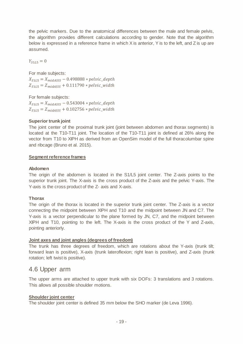
the pelvic markers. Due to the anatomical differences between the male and female pelvis,

the algorithm provides different calculations according to gender. Note that the algorithm

below is expressed in a reference frame in which X is anterior, Y is to the left, and Z is up are

assumed.

𝑌𝑆1𝐿5 = 0

For male subjects:

𝑋𝑆1𝐿5 = 𝑋𝑚𝑖𝑑𝐴𝑆𝐼𝑆 − 0.498888 ∗ 𝑝𝑒𝑙𝑣𝑖𝑐_𝑑𝑒𝑝𝑡ℎ

𝑍𝑆1𝐿5 = 𝑍𝑚𝑖𝑑𝐴𝑆𝐼𝑆 + 0.111790 ∗ 𝑝𝑒𝑙𝑣𝑖𝑐_𝑤𝑖𝑑𝑡ℎ

For female subjects:

𝑋𝑆1𝐿5 = 𝑋𝑚𝑖𝑑𝐴𝑆𝐼𝑆 − 0.543004 ∗ 𝑝𝑒𝑙𝑣𝑖𝑐_𝑑𝑒𝑝𝑡ℎ

𝑍𝑆1𝐿5 = 𝑍𝑚𝑖𝑑𝐴𝑆𝐼𝑆 + 0.102756 ∗ 𝑝𝑒𝑙𝑣𝑖𝑐_𝑤𝑖𝑑𝑡ℎ

Superior trunk joint

The joint center of the proximal trunk joint (joint between abdomen and thorax segments) is

located at the T10-T11 joint. The location of the T10-T11 joint is defined at 26% along the

vector from T10 to XIPH as derived from an OpenSim model of the full thoracolumbar spine

and ribcage (Bruno et al. 2015).

Segment reference frames

Abdomen

The origin of the abdomen is located in the S1/L5 joint center. The Z-axis points to the

superior trunk joint. The X-axis is the cross product of the Z-axis and the pelvic Y-axis. The

Y-axis is the cross product of the Z- axis and X-axis.

Thorax

The origin of the thorax is located in the superior trunk joint center. The Z-axis is a vector

connecting the midpoint between XIPH and T10 and the midpoint between JN and C7. The

Y-axis is a vector perpendicular to the plane formed by JN, C7, and the midpoint between

XIPH and T10, pointing to the left. The X-axis is the cross product of the Y and Z-axis,

pointing anteriorly.


The trunk has three degrees of freedom, which are rotations about the Y-axis (trunk tilt;

forward lean is positive), X-axis (trunk lateroflexion; right lean is positive), and Z-axis (trunk

rotation; left twist is positive).

4.6 Upper arm

The upper arms are attached to upper trunk with six DOFs: 3 translations and 3 rotations.

This allows all possible shoulder motions.

Shoulder joint center

The shoulder joint center is defined 35 mm below the SHO marker (de Leva 1996).

- 20 -

Segment reference frame

The origin of the upper arm is located at the shoulder joint center. The negative Z-axis points

towards the elbow joint center. The X-axis points anterior and is the cross-product of the Z-

axis and the mediolateral vector which is a horizontal projection of the vector from RASIS to

LASIS. The Y-axis is the cross product of the Z-axis and X-axis.


Helical angles are used (Woltring 1994) to parameterize shoulder rotation. The helical axis is

expressed in the Thorax reference frame, such that the components can be interpreted as

flexion, abduction, and internal rotation.

4.7 Forearm

Elbow joint center

The elbow joint center is the midpoint between the LEE and MEE markers.


The origin of the forearm is located in the elbow joint center. The negative Z points towards

the wrist joint center. The X-axis points anterior and is the cross-product of the Z-axis and the

mediolateral vector which is a horizontal projection of the vector from RASIS to LASIS. The

Y-axis is the cross product of the Z-axis and X-axis.


The forearm has two degrees of freedom, which are rotation around the Y-axis (elbow

flexion/extension; flexion is positive), and rotation around the Z-axis (pronation/supination;

pronation is positive). The rotation around the X-axis is set to a constant angle, determined

during the initialization pose.

4.8 Hand

Wrist joint center

The wrist joint center is the midpoint between the MW and LW markers.


The origin of the hand is located in the wrist joint center. All axes are aligned with the axes of

the forearm (hence it is important that subjects have neutral wrist angles during the

initialization pose).


The wrist has two degrees of freedom, which are rotations around the X-axis

(flexion/extension; flexion is positive), and rotations around the Y-axis (ab-/adduction;

abduction is positive). The rotation around the Z-axis is set to a constant angle, determined

during the initialization pose.

4.9 Head

Neck joint center

The neck is modeled as a single spherical joint. According to de Leva (1996), the neck

rotation center is at the spine at the level of the chin. This is defined to be on the trunk

- 21 -

midline (line from S1/L5 to mid-shoulder point during initialization pose), 2 cm above the level

of C7.


The origin of the head segment is located in the neck joint. The Z-axis points from neck joint

to THEAD. The X-axis is the cross-product of the Z-axis and the vector from RHEAD to

LHEAD, pointing anterior. The Y-axis is the cross product of the Z-axis and X-axis.


As the head is attached to the upper trunk via a single spherical joint, there are three

degrees of freedom, which are rotations around the Y-axis (head flexion/extension; flexion is

positive), the X-axis (head bend; right bend is positive), and the Z-axis (head twist; left twist

is positive).

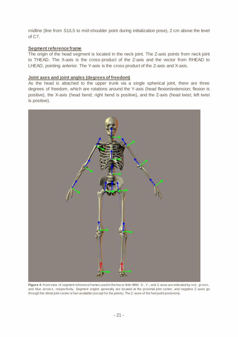
Figure 4. Front view of segment reference frames used in the low er limb HBM. X-, Y-, and Z-axes are indicated by red, green,

and blue arrow s, respectively. Segment origins generally are located at the proximal joint center, and negative Z-axes go

through the distal joint center w hen available (except for the pelvis). The Z-axes of the feet point posteriorly.

- 22 -

4.10 Mass properties

During subject initialization, mass properties of each body segment are estimated based on

segment lengths (distance between joint centers), gender, and total body mass. Segment

mass, location of the center of mass, and the inertia tensor of each segment are estimated

using parameters from Table 4 from de Leva (1996) which provides the following information:

• Segment mass as a percentage of total body mass: mperc

• Segment center of mass location as a percentage of segment length: cmperc

• Radii of gyration for the sagittal, frontal and transversal plane, expressed as a

percentage of segment length: rsag, rfro, rtra.

Segment mass (𝑚𝑠𝑒𝑔𝑚𝑒𝑛𝑡 ) is calculated from 𝑚𝑝𝑒𝑟𝑐 and the total body mass (𝑚𝑡𝑜𝑡𝑎𝑙):

𝑚𝑠𝑒𝑔𝑚𝑒𝑛𝑡 =𝑚𝑝𝑒𝑟𝑐

100∗ 𝑚𝑡𝑜𝑡𝑎𝑙 (1)

The center of mass of a given segment (𝑟𝐶𝑀) is expressed in the segment’s reference frame

and is located on the longitudinal axis:

𝑟𝐶𝑀 =𝑐𝑚𝑝𝑒𝑟𝑐

100[001

] (2)

Inertia tensors for each segment are also expressed in the segment’s reference frame:

𝐈 = 𝑚𝑠𝑒𝑔𝑚𝑒𝑛𝑡 (𝐿𝑠𝑒𝑔𝑚𝑒𝑛𝑡

100)

2

[𝑟𝑠𝑎𝑔2 0 0

0 𝑟𝑓𝑟𝑜2 0

0 0 𝑟𝑡𝑟𝑎2

] (3)

In which 𝐿𝑠𝑒𝑔𝑚𝑒𝑛𝑡 is the length of the segment.

The total body center of mass is calculated by taking the weighted average of the segment

centers of mass.

- 23 -

5. Biomechanical Analysis

Biomechanical analysis in HBM is done in five steps. First, inverse kinematics is used to

describe skeletal motion. Second, the data is low pass filtered which is needed to calculate

the first and second derivative (velocity and acceleration) without too much noise. Third, an

inverse dynamics analysis is performed to calculate the generalized forces (forces and

moments actuating the degrees of freedom). In the two final steps muscles moment arms

and muscle forces are estimated.

5.1 Kinematics

Kinematic degrees of freedom

Based on the segment description in section 4, there are 46 kinematic degrees of freedom,

and they have been given the following names. Each degree of freedom has a kinematic

variable associated with it. These are also known as “generalized coordinates”.

• PelvisX

• PelvisY

• PelvisZ

• PelvisYaw

• PelvisForwardPitch

• PelvisRightRoll

• TrunkFlexion

• TrunkRightBend

• TrunkLeftTwist

• HeadFlexion

• HeadRightBend

• HeadLeftTwist

• RShoulderUp

• RShoulderForward

• RShoulderInward

• RShoulderFlexion

• RShoulderAbduction

• RSchoulderInternalRotation

• RElbowFlexion

• RForeArmPronation

• RWristFlexion

• RHandAbduction

• LShoulderUp

• LShoulderForward

• LShoulderInward

• LShoulderFlexion

• LShoulderAbduction

• LSchoulderInternalRotation

• LElbowFlexion

• LForeArmPronation

• LWristFlexion

- 24 -

• LHandAbduction

• RHipFlexion

• RHipAbduction

• RHipInternalRotation

• RkneeFlexion

• RAnklePlantarFlexion

• RFootPronation

• RToeFlexion

• LHipFlexion

• LHipAbduction

• LHipInternalRotation

• LKneeFlexion

• LAnklePlantarFlexion

• LFootPronation

• LToeFlexion

Inverse kinematics

In contrast to conventional models that calculate each segment independently using at least

three markers per segment, the inverse kinematics in HBM are calculated all at once. During

static calibration HBM determines the segment reference frames based on the marker

positions. For each real-time frame these segments are fitted onto the marker data by

minimizing the error between the marker data and the segment orientations. Because all

available markers are used in this optimization, fewer markers are required per segment than

in the conventional models. Technically HBM would only require the anatomical markers

(bold in Table 1) to solve kinematics. However, additional technical markers are added to

HBM (Table 1) to provide redundancy and robustness for the model in case of marker drop

outs.

The inverse kinematics is based on van den Bogert & Su (2008). The skeleton model is

defined with 46 DOF, represented by the generalized coordinates 𝒒 = [𝒒1 … 𝒒21]𝑇, in which

for example 𝑞1 is PelvisX, q2 is PelvisY, etcetera (see above). Since all segment reference

frames are known from the marker data, the position vector 𝒓 = [𝑥, 𝑦, 𝑧]𝑇 and orientation

matrix 𝑹 of each segment expressed in the global reference frame can be computed as a

function of 𝒒. Furthermore, the position of each marker in the segment reference frame (𝒑) is

known. Therefore, the coordinates of each marker in the global reference frame can be

expressed as a function of 𝒒, by adding 𝑹(𝒒) ∙ 𝒑 (i.e. the position of a marker in the segment

reference frame, rotated to the global reference frame) to the position vector of the segment

origin in the global reference frame (𝒓(𝒒)). Thus, the position of a certain marker 𝑖 in the

global reference frame is

𝒓𝑖 = 𝒓(𝒒) + 𝑹(𝒒) ∙ 𝒑𝑖 ≡ 𝒇𝑖(𝒒) (5)

The optimal estimate for the skeleton pose 𝒒 can then be obtained by minimizing the

squared difference between the measured coordinates of the markers in the global reference

frame and their position expressed as a function of 𝒒. If 𝑀 markers are placed, the

optimization is

- 25 -

𝑭(𝒒) = ∑ ‖𝒓𝑖 − 𝒇𝑖(𝒒)‖2𝑀𝑖=1 (6)

Note that in three dimensions, the right hand side is a sum of 3𝑀 squares, since the squares

of x, y, and z distances are added. This optimization method is known as global optimization

(Lu & O’Connor 1999), in which global refers to the fact that the entire skeleton is modeled at

once, instead of modeling each segment individually. This makes the model less sensitive to

marker drop-outs and skin artifacts. In HBM, equation 6 is minimized using the Levenberg-

Marquardt algorithm, adapted from Numerical Recipes (Press et al. 1992). In this way, the

generalized coordinates (𝒒) for each frame are calculated within 1ms of computation time.

Filtering and differentiation

The calculation of joint moments and muscle forces depends on the acceleration and velocity

of the skeleton, which are the first and second derivative of skeleton movement (𝒒). To

prevent these derivatives from being too noisy, 𝒒 has to be smoothed using a filter.

The HBM software has a built-in real-time 2nd order low pass Butterworth filter. Higher order

filters may reject noise better, but will also increase the time delay. Therefore, the used filter

is considered to be a good compromise to be used in HBM. The state variable technique is

used instead of the more common recursive digital filter, which allows processing data with

varying sample rates (which occurs if the motion capture system drops a frame).

Furthermore, this technique automatically generates first and second derivatives.

The cutoff frequency of the filter can be adjusted by the user to a maximum of 20 Hz. Higher

frequencies are not allowed because these are unnecessary for human movement and

would increase computation time. The default cutoff frequency is set to 6Hz, since this was

found to be the highest frequency in kinematics related to gait (Winter et al. 1974). To

prevent artifacts in joint movements, force plate data are processed with the same low pass

filter as the kinematics (van den Bogert & De Koning 1996; Bisseling & Hof 2006).

5.2 Kinetics

Generalized forces

Each DOF is actuated with a force (for translational DOFs) or moment (for rotational DOFs).

These forces and moments are also known as “generalized forces”. The signs of these are

defined such that a positive force or moment would generate a movement in which the

corresponding generalized coordinate is increasing. These (internal) moments and forces are

solved using inverse dynamics. Furthermore, mechanical work can be computed as the

product of the amount of change in the generalized coordinate and the amount of

generalized force. The powers are presented per joint axis as most of the literature that

reports on joint power presents a 2D sagittal plane analysis. When comparing HBM results

with those results, only the flexion-extension power should be used. If preferred, the

individual powers per joint can easily be summed to calculate the total joint power since they

are scalars.

There is one exception to the correspondence between generalized coordinates and

generalized forces: pelvis moments have been defined as Cartesian XYZ components in the

world reference frame, rather than as moments on the yaw, pitch, and roll axes. Thus, the

first six generalized forces are residual loads exerted by the outside world on the pelvis.

- 26 -

When all external forces are measured and accounted for in the inverse dynamics, these

loads should be zero.

Inverse dynamics

The generalized forces are calculated in an inverse dynamic analysis, which has the low

pass filtered kinematics and the ground reaction forces as input. Like the inverse kinematic

solution does for the generalized coordinates, the inverse dynamic analysis calculates all

generalized forces (𝝉) at once using the following equation from van den Bogert et al. (2013):

𝝉 = 𝑴(𝒒)�̈� + 𝒄(𝒒, �̇�) + 𝑩(𝒒)𝝉𝒆𝒙𝒕 (7)

In this equation 𝑴 is a square matrix containing mass properties of the segments, 𝒄 are

terms related to Coriolis and centrifugal effects and gravity, and 𝑩(𝒒)𝝉𝒆𝒙𝒕 are the measured

external forces (force plate data).

It is assumed that full ground reaction force data is available. When two force plates are used

and each plate registers 3D forces and 3D moments, 𝝉𝒆𝒙𝒕 contains 12 variables. Furthermore

it is assumed that all DOFs of the model are actuated, which implies that 𝝉 contains one

variable for each DOF of the model. Thus, the solution also includes 3D force and moment

acting on the root segment (pelvis). These values will be non-zero, even though it is known

these values are exactly zero. Allowing this error has the advantage that there is an exact

solution for 𝝉. Also, joint moments are only influenced by inertial effects distal to the joint.

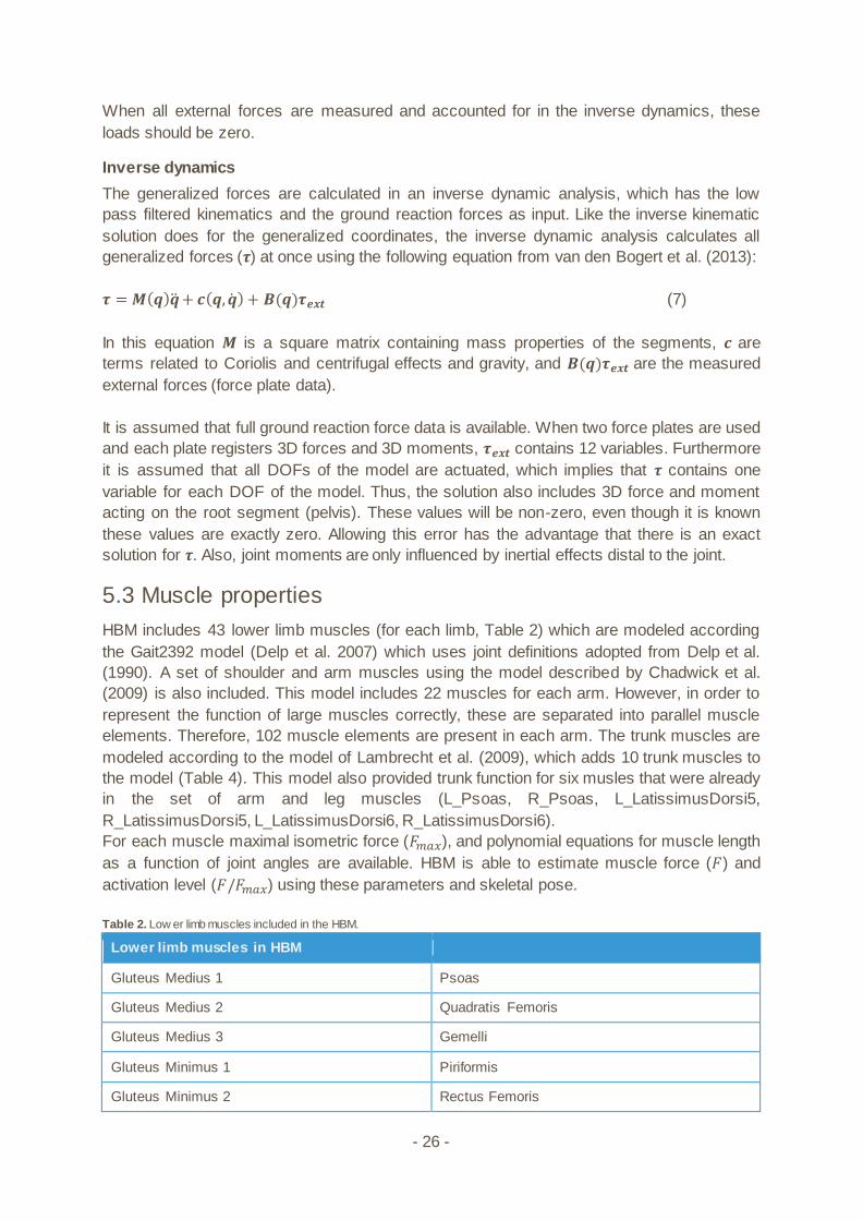
5.3 Muscle properties

HBM includes 43 lower limb muscles (for each limb, Table 2) which are modeled according

the Gait2392 model (Delp et al. 2007) which uses joint definitions adopted from Delp et al.

(1990). A set of shoulder and arm muscles using the model described by Chadwick et al.

(2009) is also included. This model includes 22 muscles for each arm. However, in order to

represent the function of large muscles correctly, these are separated into parallel muscle

elements. Therefore, 102 muscle elements are present in each arm. The trunk muscles are

modeled according to the model of Lambrecht et al. (2009), which adds 10 trunk muscles to

the model (Table 4). This model also provided trunk function for six musles that were already

in the set of arm and leg muscles (L_Psoas, R_Psoas, L_LatissimusDorsi5,

R_LatissimusDorsi5, L_LatissimusDorsi6, R_LatissimusDorsi6).

For each muscle maximal isometric force (𝐹𝑚𝑎𝑥), and polynomial equations for muscle length

as a function of joint angles are available. HBM is able to estimate muscle force (𝐹) and

activation level (𝐹/𝐹𝑚𝑎𝑥) using these parameters and skeletal pose.

Table 2. Low er limb muscles included in the HBM.

Lower limb muscles in HBM

Gluteus Medius 1 Psoas

Gluteus Medius 2 Quadratis Femoris

Gluteus Medius 3 Gemelli

Gluteus Minimus 1 Piriformis

Gluteus Minimus 2 Rectus Femoris

- 27 -

Gluteus Minimus 3 Biceps Femoris SH

Semimembranosus Vastus Medialis

Semitendinosus Vastus Intermedius

Biceps Femoris LH Vastus Lateralis

Sartorius Medial Gastrocnemius

Adductor Longus Lateral Gastrocnemius

Adductor Brevis Soleus

Adductor Magnus 1 Tibialis Posterior

Adductor Magnus 2 Flexor Digitorum Longus

Adductor Magnus 3 Flexor Hallicus Longus

Tensor Fascia Lata Tibialis Anterior

Pectineus Peroneus Brevis

Gracilis Peroneus Longus

Gluteus Maximus 1 Peroneus Tertius

Gluteus Maximus 2 Extensor Digitorum Longus

Gluteus Maximus 3 Extensor Hallicus Longus

Iliacus

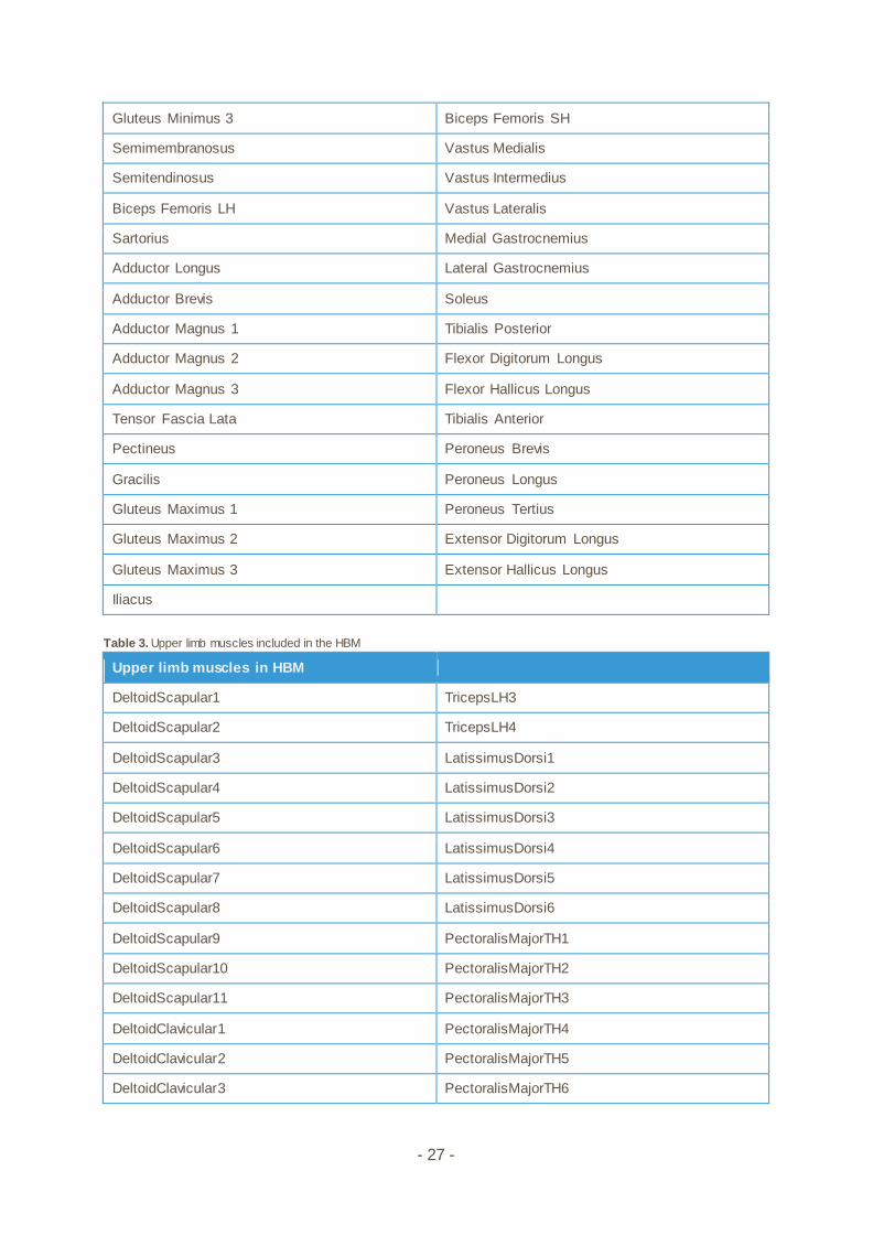
Table 3. Upper limb muscles included in the HBM

Upper limb muscles in HBM

DeltoidScapular1 TricepsLH3

DeltoidScapular2 TricepsLH4

DeltoidScapular3 LatissimusDorsi1






DeltoidScapular9 PectoralisMajorTH1



DeltoidClavicular1 PectoralisMajorTH4



- 28 -

DeltoidClavicular4 PectoralisMajorCH1

CoracoBrachialis1 PectoralisMajorCH2

CoracoBrachialis2 TricepsMedH1

CoracoBrachialis3 TricepsMedH2

Infraspinatus1 TricepsMedH3



Infraspinatus4 Brachialis1



TeresMinor1 Brachialis4



TeresMajor1 Brachialis7

TeresMajor2 Brachioradialis1



Supraspinatus1 PronatorTeres1

Supraspinatus2 PronatorTeres2

Supraspinatus3 Supinator1

Supraspinatus4 Supinator2

Subscapularis1 Supinator3



Subscapularis4 PronatorQuadratus1



Subscapularis7 TricepsLatH1





BicepsBrachiiLH Anconeus1

BicepsBrachiiSH1 Anconeus2

- 29 -

BicepsBrachiiSH2 Anconeus3

TricepsLH1 Anconeus4

TricepsLH2 Anconeus5

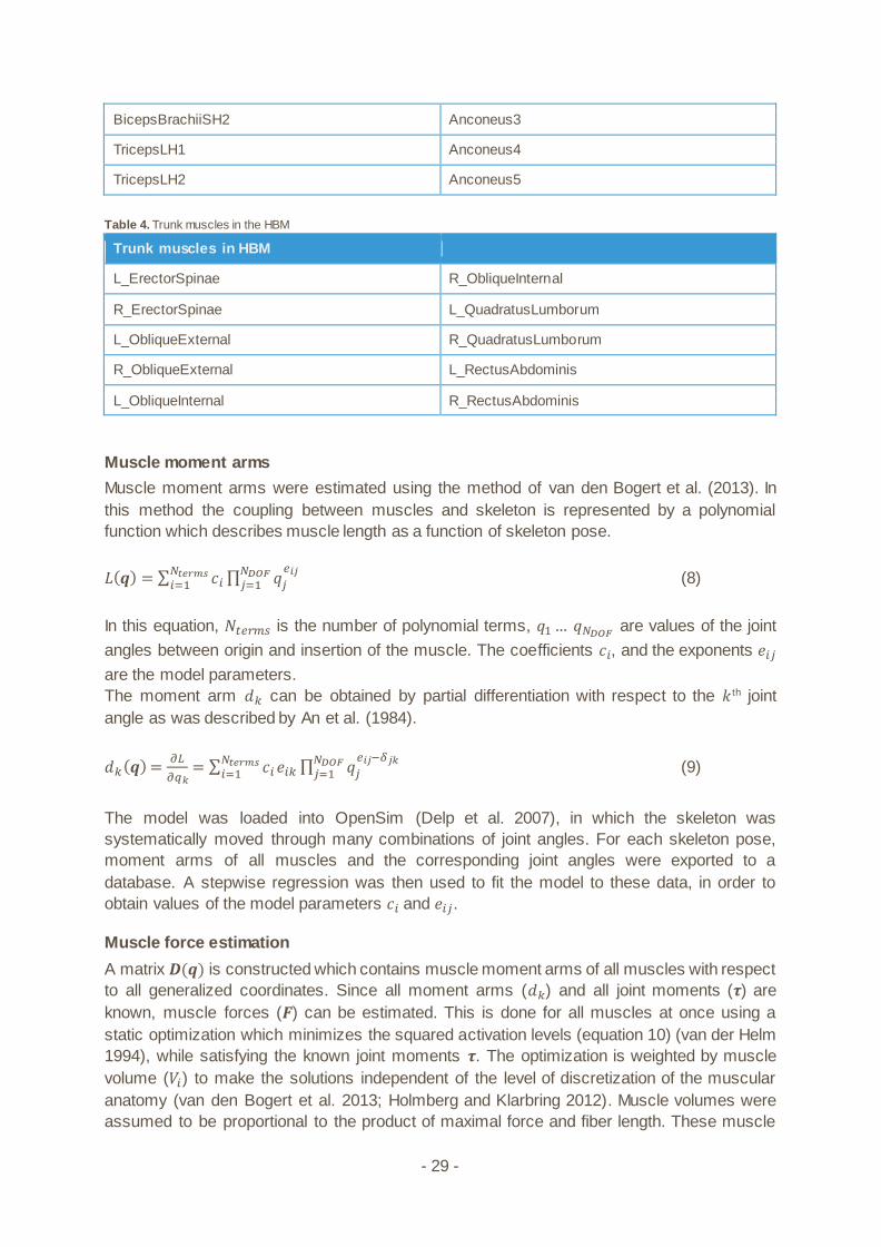
Table 4. Trunk muscles in the HBM

Trunk muscles in HBM

L_ErectorSpinae R_ObliqueInternal

R_ErectorSpinae L_QuadratusLumborum

L_ObliqueExternal R_QuadratusLumborum

R_ObliqueExternal L_RectusAbdominis

L_ObliqueInternal R_RectusAbdominis

Muscle moment arms

Muscle moment arms were estimated using the method of van den Bogert et al. (2013). In

this method the coupling between muscles and skeleton is represented by a polynomial

function which describes muscle length as a function of skeleton pose.

𝐿(𝒒) = ∑ 𝑐𝑖𝑁𝑡𝑒𝑟𝑚𝑠𝑖=1

∏ 𝑞𝑗

𝑒𝑖𝑗𝑁𝐷𝑂𝐹𝑗=1 (8)

In this equation, 𝑁𝑡𝑒𝑟𝑚𝑠 is the number of polynomial terms, 𝑞1 … 𝑞𝑁𝐷𝑂𝐹 are values of the joint

angles between origin and insertion of the muscle. The coefficients 𝑐𝑖, and the exponents 𝑒𝑖𝑗

are the model parameters.

The moment arm 𝑑𝑘 can be obtained by partial differentiation with respect to the 𝑘 th joint

angle as was described by An et al. (1984).

𝑑𝑘(𝒒) =𝜕𝐿

𝜕𝑞𝑘= ∑ 𝑐𝑖

𝑁𝑡𝑒𝑟𝑚𝑠𝑖=1 𝑒𝑖𝑘 ∏ 𝑞𝑗

𝑒𝑖𝑗−𝛿𝑗𝑘𝑁𝐷𝑂𝐹𝑗=1 (9)

The model was loaded into OpenSim (Delp et al. 2007), in which the skeleton was

systematically moved through many combinations of joint angles. For each skeleton pose,

moment arms of all muscles and the corresponding joint angles were exported to a

database. A stepwise regression was then used to fit the model to these data, in order to

obtain values of the model parameters 𝑐𝑖 and 𝑒𝑖𝑗.

Muscle force estimation

A matrix 𝑫(𝒒) is constructed which contains muscle moment arms of all muscles with respect

to all generalized coordinates. Since all moment arms (𝑑𝑘) and all joint moments (𝝉) are

known, muscle forces (𝑭) can be estimated. This is done for all muscles at once using a

static optimization which minimizes the squared activation levels (equation 10) (van der Helm

1994), while satisfying the known joint moments 𝝉. The optimization is weighted by muscle

volume (𝑉𝑖) to make the solutions independent of the level of discretization of the muscular

anatomy (van den Bogert et al. 2013; Holmberg and Klarbring 2012). Muscle volumes were

assumed to be proportional to the product of maximal force and fiber length. These muscle

- 30 -

properties were taken from the original models (Chadwick et al. 2009; Delp et al. 1990;

Lambrecht et al. 2009).

𝑭 = ∑ 𝑉𝑖 (𝐹𝑖

𝐹𝑚𝑎𝑥)

2𝑛𝑖=1 (10)

Subject to linear equality constraints

𝑫(𝒒)𝑭 = 𝝉

And bound constraints

𝐹𝑖 ≥ 0

This is a quadratic programming problem, which is solved in HBM in real time using a

recurrent neural network as described by Xia & Feng (2005).

Activation levels are guaranteed to be positive, but are not guaranteed to be less than 1. The

𝐹𝑚𝑎𝑥 values used in the optimization are derived from cadaveric data (Delp et al. 1990).

These values are meant to be interpreted as relative muscle strengths, so activation levels

may be higher than 1 when capturing above average strong subjects.

- 31 -

6. References

An, K.N. et al., 1984. Determination of muscle orientations and moment arms. Journal of biomechanical engineering, 106(3), pp.280–2.

Assi, A. et al., 2016. Validation of hip joint center localization methods during gait analysis using 3D EOS imaging in typically developing and cerebral palsy children. Gait and Posture, 48, pp.30–35.

Bell, A.L., Brand, R.A. & Pedersen, D.R., 1989. Prediction of hip joint centre location from external landmarks. Human Movement Science, 8(1), pp.3–16.

Bisseling, R.W. & Hof, A.L., 2006. Handling of impact forces in inverse dynamics. Journal of Biomechanics, 39(13), pp.2438–2444.

van den Bogert, A.J. et al., 2013. A real-time system for biomechanical analysis of human movement and muscle function. Medical & Biological Engineering & Computing, 51(10), pp.1069–1077.

van den Bogert, A.J. & De Koning, J.J., 1996. On optimal filtering for inverse dynamics analysis. In Proceedings of the IXth biennial conference of the Canadian society for biomechanics. pp. 214–215.

van den Bogert, A.J., Smith, G.D. & Nigg, B.M., 1994. In vivo determination of the anatomical axes of the ankle joint complex: An optimization approach. Journal of Biomechanics, 27(12), pp.1477–1488.

van den Bogert, A.J. & Su, A., 2008. A weighted least squares method for inverse dynamic analysis. Computer methods in biomechanics and biomedical engineering, 11(1), pp.3–9.

Bruno, A.G., Bouxsein, M.L. & Anderson, D.E., 2015. Development and Validation of a Musculoskeletal Model of the Fully Articulated Thoracolumbar Spine and Rib Cage. Journal of biomechanical engineering, 137(8), p.81003.

Burdett, R.G., 1982. Forces predicted at the ankle during running. Medicine and science in sports and exercise, 14(4), pp.308–316.

Camomilla, V. et al., 2006. An optimized protocol for hip joint centre determination using the functional method. Journal of Biomechanics, 39(6), pp.1096–1106.

van Campen, A. et al., 2011. Functional knee axis based on isokinetic dynamometry data: Comparison of two methods, MRI validation, and effect on knee joint kinematics. Journal of Biomechanics, 44(15), pp.2595–2600.

Chadwick, E.K. et al., 2009. A Real-Time, 3-D Musculoskeletal Model for Dynamic Simulation of Arm Movements. Biomedical Engineering, IEEE Transactions on, 56(4), pp.941–948.

Delp, S.L. et al., 1990. An Interactive Graphics-Based Model of the Lower Extremity to Study Orthopaedic Surgical Procedures. IEEE Transactions on Biomedical Engineering, 37(8), pp.757–767.

Delp, S.L. et al., 2007. OpenSim: Open source to create and analyze dynamic simulations of movement. IEEE transactions on bio-medical engineering, 54(11), pp.1940–1950.

Gamage, S.S.H.U. & Lasenby, J., 2002. New least squares solutions for estimating the average centre of rotation and the axis of rotation. Journal of Biomechanics, 35(1), pp.87–93.

Glitsch, U. & Baumann, W., 1997. The three-dimensional determination of internal loads in the lower extremity. Journal of Biomechanics, 30(11–12), pp.1123–1131.

Halvorsen, K., 2003. Bias compensated least squares estimate of the center of rotation. Journal of Biomechanics, 36(7), pp.999–1008.

Harrington, M.E. et al., 2007. Prediction of the hip joint centre in adults, children, and patients with cerebral palsy based on magnetic resonance imaging. Journal of Biomechanics, 40, pp.595–602.

van der Helm, F.C.T., 1994. A finite element musculoskeletal model of the shoulder mechanism. Journal of Biomechanics, 27(5), pp.551–569.

Holmberg, L.J. & Klarbring, A., 2012. Muscle decomposition and recruitment criteria

- 32 -

influence muscle force estimates. Multibody System Dynamics, 28(3), pp.283–289. Isman, R. & Inman, V., 1969. Anthropometric Studies of the Human Foot and Ankle. Foot

And Ankle, 11, pp.97–129. Kainz, H. et al., 2015. Estimation of the hip joint centre in human motion analysis: A

systematic review. Clinical Biomechanics, 30(4), pp.319–329. Kainz, H. et al., 2016. Joint kinematic calculation based on clinical direct kinematic versus

inverse kinematic gait models. Journal of Biomechanics, 49(9), pp.1658–1669. Lambrecht, J.M. et al., 2009. Musculoskeletal model of trunk and hips for development of

seated-posture-control neuroprosthesis. Journal of rehabilitation research and development, 46(4), pp.515–28.

Leardini, A. et al., 1999. Validation of a functional method for the estimation of hip joint centre location. Journal of Biomechanics, 32(1), pp.99–103.

de Leva, P., 1996. Adjustments to Zatsiorsky-Seluyanov’s segment inertia parameters. Journal of biomechanics, 29(9), pp.1223–1230.

Lu, T.W. & O’Connor, J.J., 1999. Bone position estimation from skin marker co-ordinates using global optimisation with joint constraints. Journal of Biomechanics, 32(2), pp.129–134.

MacWilliams, B. a., 2008. A comparison of four functional methods to determine centers and axes of rotations. Gait and Posture, 28(4), pp.673–679.

Peters, A. et al., 2012. A comparison of hip joint centre localisation techniques with 3-DUS for clinical gait analysis in children with cerebral palsy. Gait and Posture, 36(2), pp.282–286.

Press, W.H. et al., 1992. Numerical recipes in C (2nd ed.): the art of scientific computing, Ramakrishnan, H.K. & Kadaba, M.P., 1991. On the estimation of joint kinematics during gait.

Journal of biomechanics, 24(10), pp.969–977. Reynolds, H.M., Snow, C.C. & Young, J.W., 1982. Spatial geometry of the human pelvis,

Oklahoma City: DTIC Document. Sangeux, M., Peters, A. & Baker, R., 2011. Hip joint centre localization: Evaluation on normal

subjects in the context of gait analysis. Gait and Posture, 34(3), pp.324–328. Sangeux, M., Pillet, H. & Skalli, W., 2014. Which method of hip joint centre localisation

should be used in gait analysis? Gait and Posture, 40, pp.20–25. Winter, D.A., Sidwall, H.G. & Hobson, D.A., 1974. Measurement and reduction of noise in

kinematics of locomotion. Journal of Biomechanics, 7(2), pp.157–159. Woltring, H.J., 1994. 3-D attitude representation of human joints: A standardization proposal.

Journal of Biomechanics, 27(12), pp.1399–1414. Wu, G. et al., 2002. ISB recommendation on definitions of joint coordinate system of various

joints for the reporting of human joint motion--part I: ankle, hip, and spine. International Society of Biomechanics. Journal of biomechanics, 35, pp.543–548.

Wu, G. et al., 2005. ISB recommendation on definitions of joint coordinate systems of various joints for the reporting of human joint motion -- Part II: Shoulder, elbow, wrist and hand. Journal of Biomechanics, 38(5), pp.981–992.

Wu, G. & Cavanagh, P.R., 1995. ISB Recommendations in the Reporting for Standardization of Kinematic Data. J Biomechanics, 28(10), pp.1257–1261.

Xia, Y. & Feng, G., 2005. An improved neural network for convex quadratic optimization with application to real-time beamforming. Neurocomputing, 64(1–4 SPEC. ISS.), pp.359–374.

Hogehilweg 18 - C | 1101 CD | Amsterdam | The Netherlands

T: +31(0)20 301 30 20 | www.motekforcelink.com

hbm2 - reference manual

Documents