hdr imaging and the bilateral filter - computer … · hdr imaging and the bilateral filter frédo...
TRANSCRIPT

HDR imaging and the Bilateral Filter
Frédo DurandMIT - EECS
Tuesday, January 26, 2010

Leica discussion• Photographers discuss what features they want in
future Leica cameras– http://luminous-landscape.com/essays/leica-open-letter.shtml– http://luminous-landscape.com/essays/leica-different-view.shtml– http://luminous-landscape.com/essays/hogan-leica.shtml
• Inspiring for class projects on focusing & metering
From http://luminous-landscape.com/essays/leica-open-letter.shtml
Tuesday, January 26, 2010
! 2010 Marc Levoy
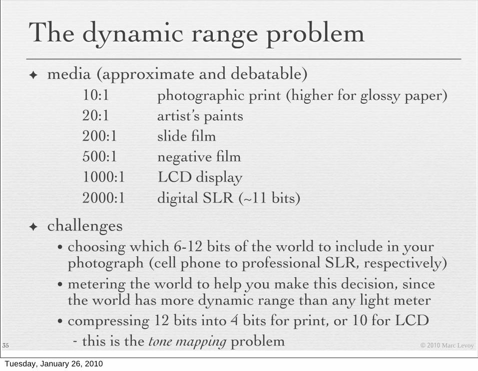
The dynamic range problem! media (approximate and debatable)
10:1!! ! photographic print (higher for glossy paper)20:1!! ! artist’s paints200:1! ! slide film500:1! ! negative film1000:1!! LCD display2000:1!! digital SLR (~11 bits)
! challenges• choosing which 6-12 bits of the world to include in your
photograph (cell phone to professional SLR, respectively)• metering the world to help you make this decision, since
the world has more dynamic range than any light meter• compressing 12 bits into 4 bits for print, or 10 for LCD
- this is the tone mapping problem35
Tuesday, January 26, 2010
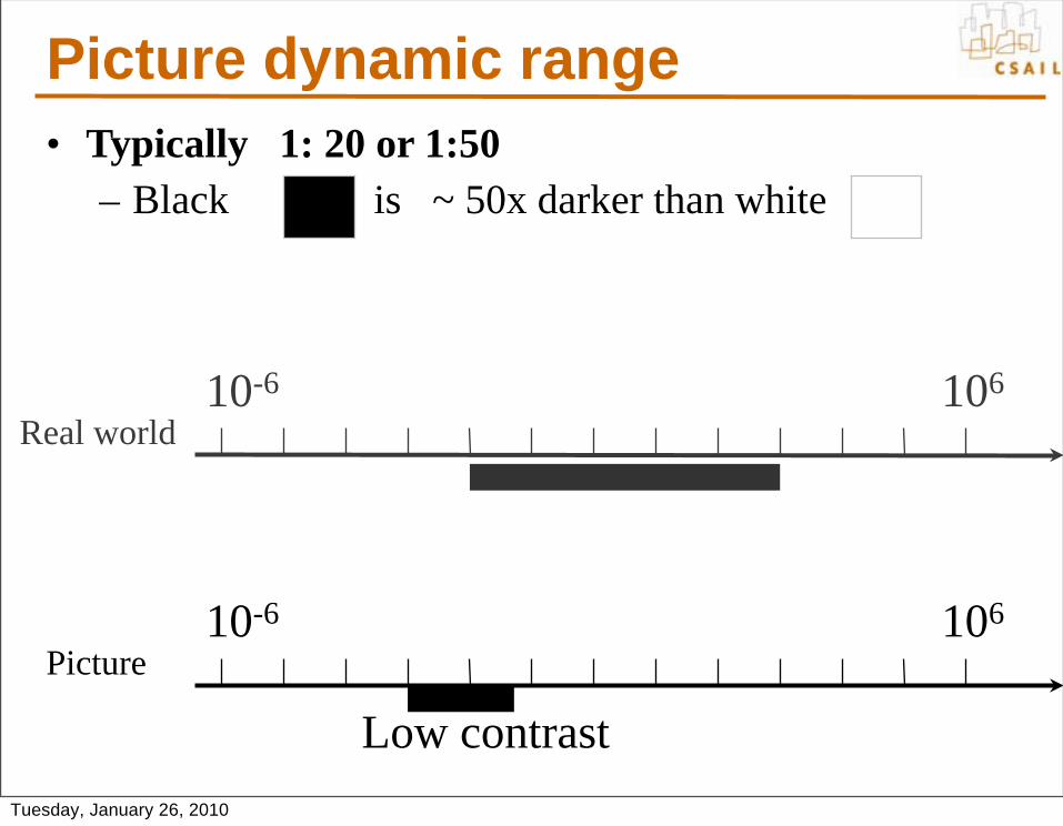
Picture dynamic range• Typically 1: 20 or 1:50
– Black is ~ 50x darker than white
10-6 106
10-6 106
Real world
Picture
Low contrastTuesday, January 26, 2010
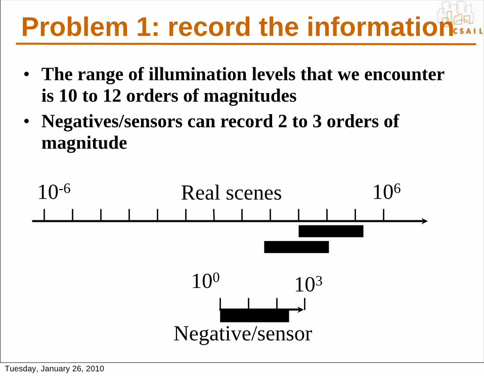
Problem 1: record the information• The range of illumination levels that we encounter
is 10 to 12 orders of magnitudes• Negatives/sensors can record 2 to 3 orders of
magnitude
10-6 106
100
Negative/sensor
103
Real scenes
Tuesday, January 26, 2010
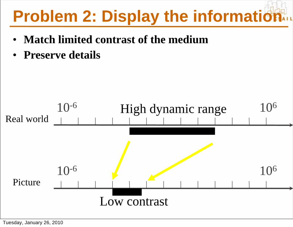
Problem 2: Display the information• Match limited contrast of the medium• Preserve details
10-6 106
10-6 106
Real world
Picture
Low contrast
High dynamic range
Tuesday, January 26, 2010

Without HDR & tone mapping
Tuesday, January 26, 2010
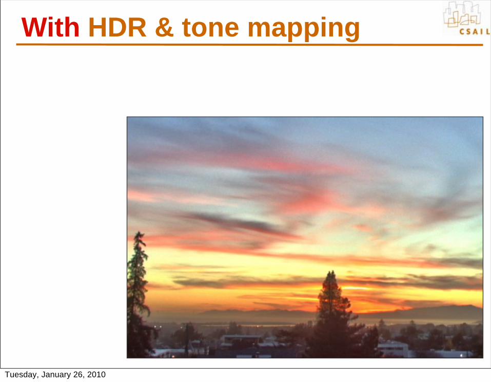
With HDR & tone mapping
Tuesday, January 26, 2010
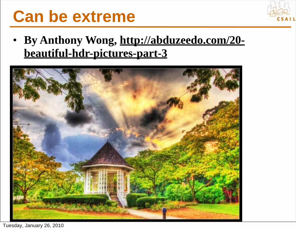
Can be extreme• By Anthony Wong, http://abduzeedo.com/20-
beautiful-hdr-pictures-part-3
Tuesday, January 26, 2010

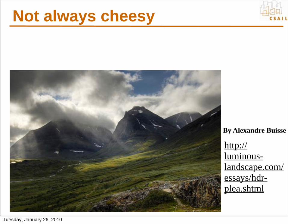
Not always cheesy
By Alexandre Buisse
http://luminous-landscape.com/essays/hdr-plea.shtml
Tuesday, January 26, 2010
Not always cheesy
By Alexandre Buisse
http://luminous-landscape.com/essays/hdr-plea.shtml
Tuesday, January 26, 2010

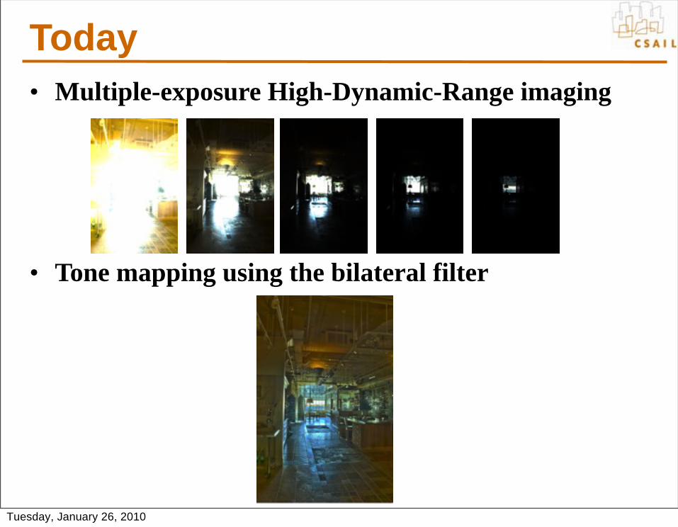
Today• Multiple-exposure High-Dynamic-Range imaging
• Tone mapping using the bilateral filter
Tuesday, January 26, 2010
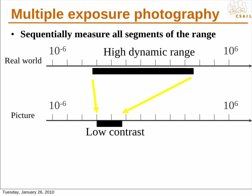
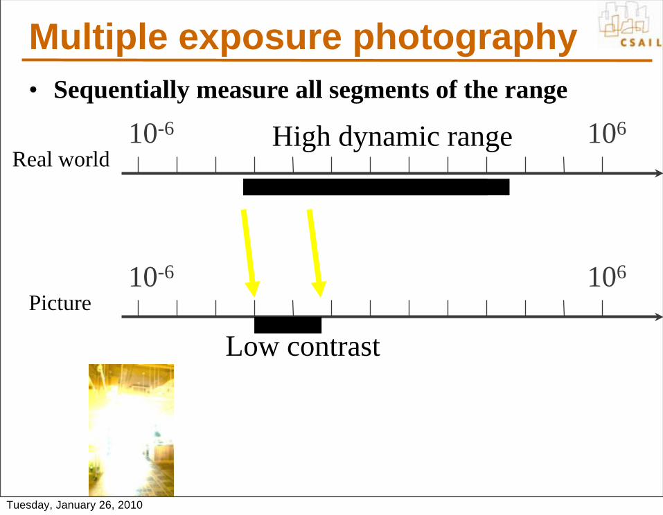
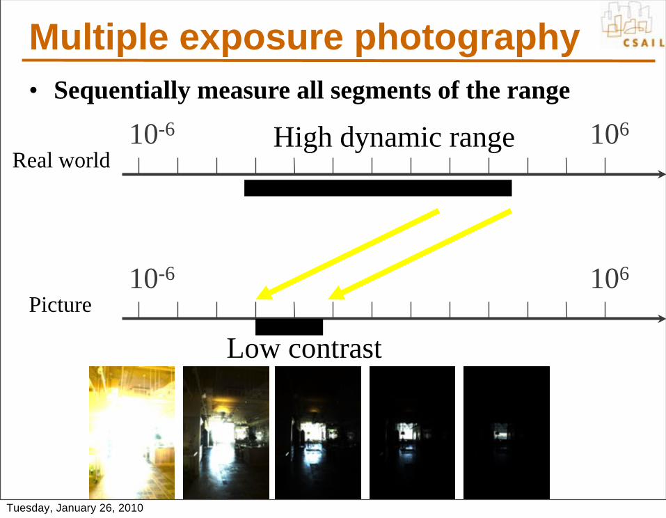
Multiple exposure photography• Sequentially measure all segments of the range
10-6 106
10-6 106
Real world
Picture
Low contrast
High dynamic range
Tuesday, January 26, 2010
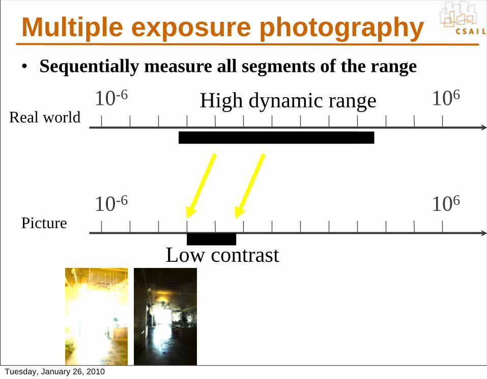
Multiple exposure photography• Sequentially measure all segments of the range
10-6 106
10-6 106
Real world
Picture
Low contrast
High dynamic range
Tuesday, January 26, 2010
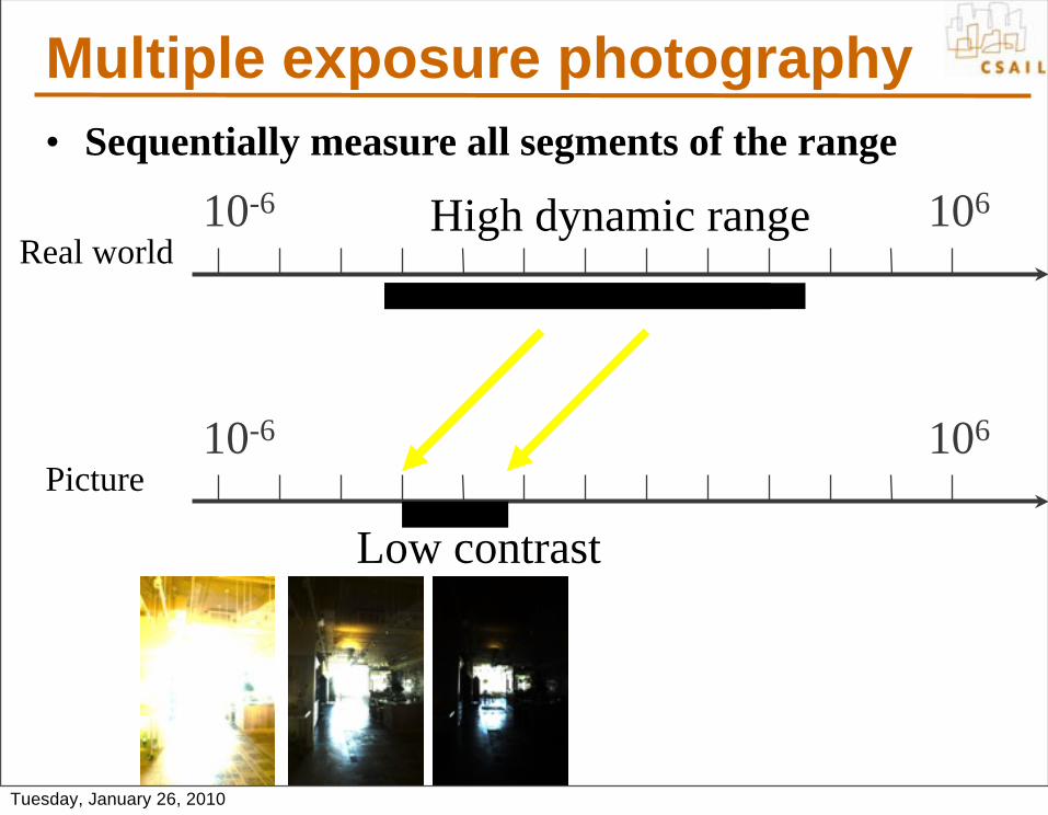
Multiple exposure photography• Sequentially measure all segments of the range
10-6 106
10-6 106
Real world
Picture
Low contrast
High dynamic range
Tuesday, January 26, 2010
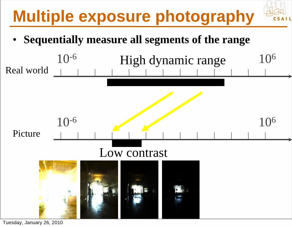
Multiple exposure photography• Sequentially measure all segments of the range
10-6 106
10-6 106
Real world
Picture
Low contrast
High dynamic range
Tuesday, January 26, 2010
Multiple exposure photography• Sequentially measure all segments of the range
10-6 106
10-6 106
Real world
Picture
Low contrast
High dynamic range
Tuesday, January 26, 2010
Multiple exposure photography• Sequentially measure all segments of the range
10-6 106
10-6 106
Real world
Picture
Low contrast
High dynamic range
Tuesday, January 26, 2010
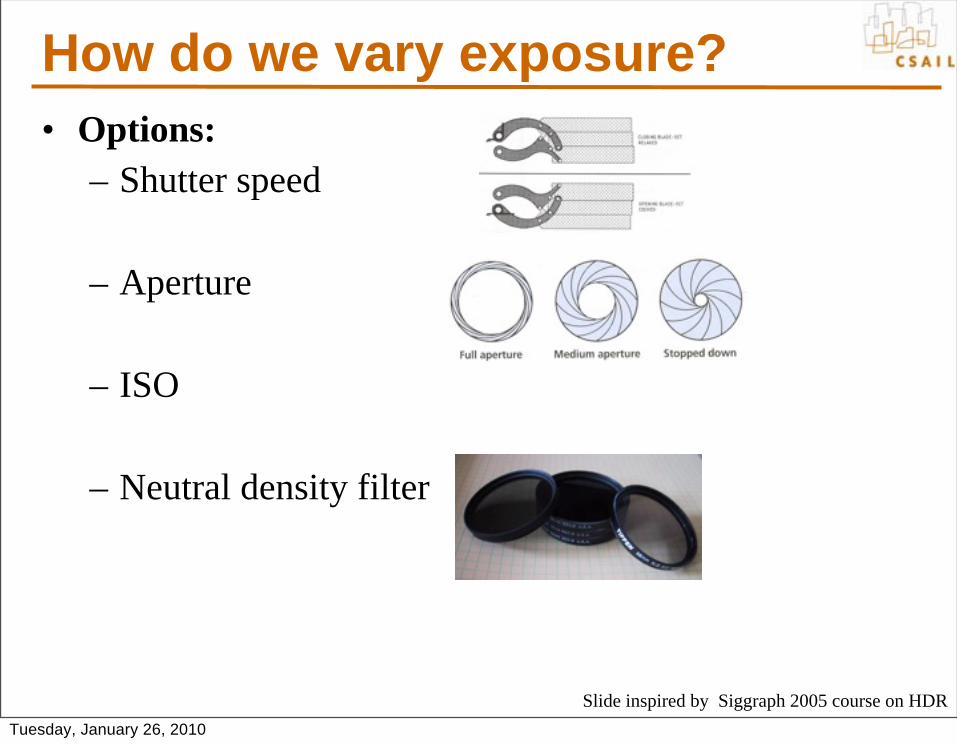
How do we vary exposure? • Options:
– Shutter speed
– Aperture
– ISO
– Neutral density filter
Slide inspired by Siggraph 2005 course on HDRTuesday, January 26, 2010
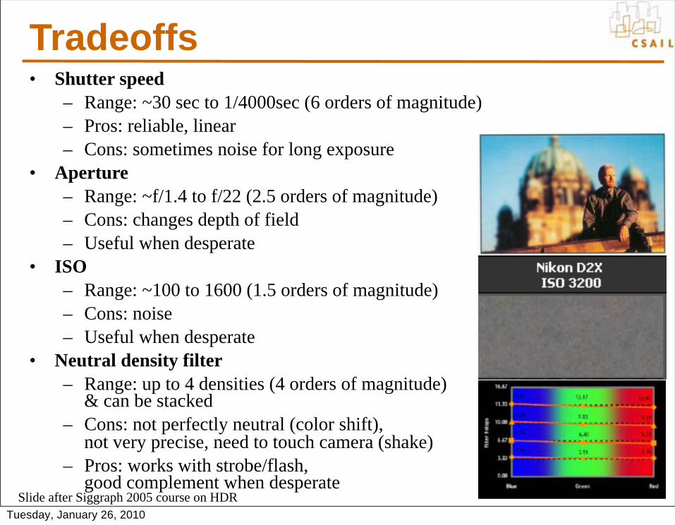
Tradeoffs• Shutter speed
– Range: ~30 sec to 1/4000sec (6 orders of magnitude)– Pros: reliable, linear– Cons: sometimes noise for long exposure
• Aperture– Range: ~f/1.4 to f/22 (2.5 orders of magnitude)– Cons: changes depth of field– Useful when desperate
• ISO– Range: ~100 to 1600 (1.5 orders of magnitude)– Cons: noise– Useful when desperate
• Neutral density filter– Range: up to 4 densities (4 orders of magnitude)
& can be stacked– Cons: not perfectly neutral (color shift),
not very precise, need to touch camera (shake)– Pros: works with strobe/flash,
good complement when desperateSlide after Siggraph 2005 course on HDR
Tuesday, January 26, 2010

Questions?
Tuesday, January 26, 2010

HDR image using multiple exposure• Given N photos at different exposure• Recover a HDR color for each pixel
• We’ll study Debevec and Malik’s 97 algorithm– http://www.debevec.org/Research/HDR/
Tuesday, January 26, 2010
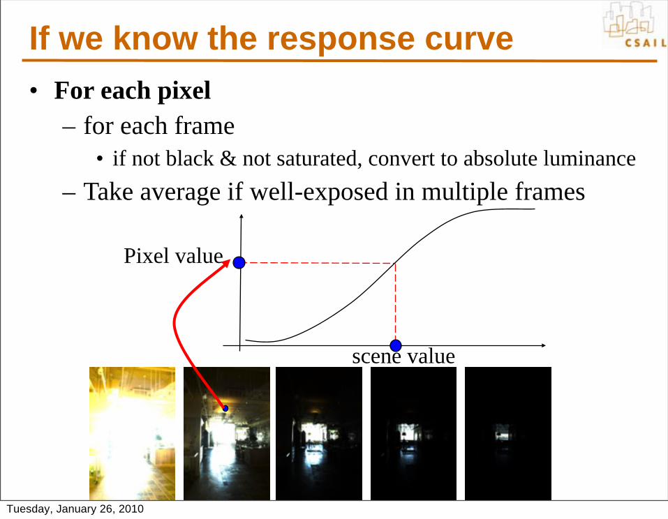
If we know the response curve• For each pixel
– for each frame• if not black & not saturated, convert to absolute luminance
– Take average if well-exposed in multiple frames
Pixel value
scene value
Tuesday, January 26, 2010
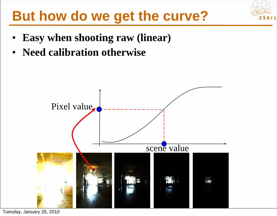
But how do we get the curve? • Easy when shooting raw (linear)• Need calibration otherwise
Pixel value
scene value
Tuesday, January 26, 2010
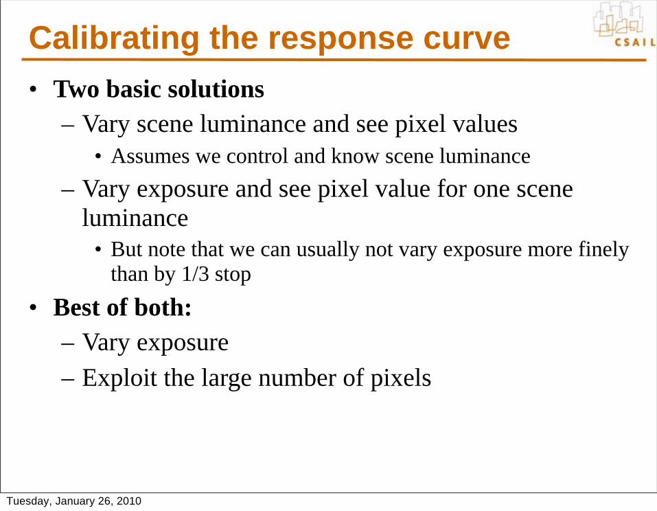
Calibrating the response curve• Two basic solutions
– Vary scene luminance and see pixel values• Assumes we control and know scene luminance
– Vary exposure and see pixel value for one scene luminance
• But note that we can usually not vary exposure more finely than by 1/3 stop
• Best of both: – Vary exposure– Exploit the large number of pixels
Tuesday, January 26, 2010
• 3
• 1• 2
Δt =1/100 sec
• 3
• 1 • 2
Δt =1 sec
• 3
• 1• 2
Δt =1/1000 sec
• 3
• 1 •
2
Δt =10 sec
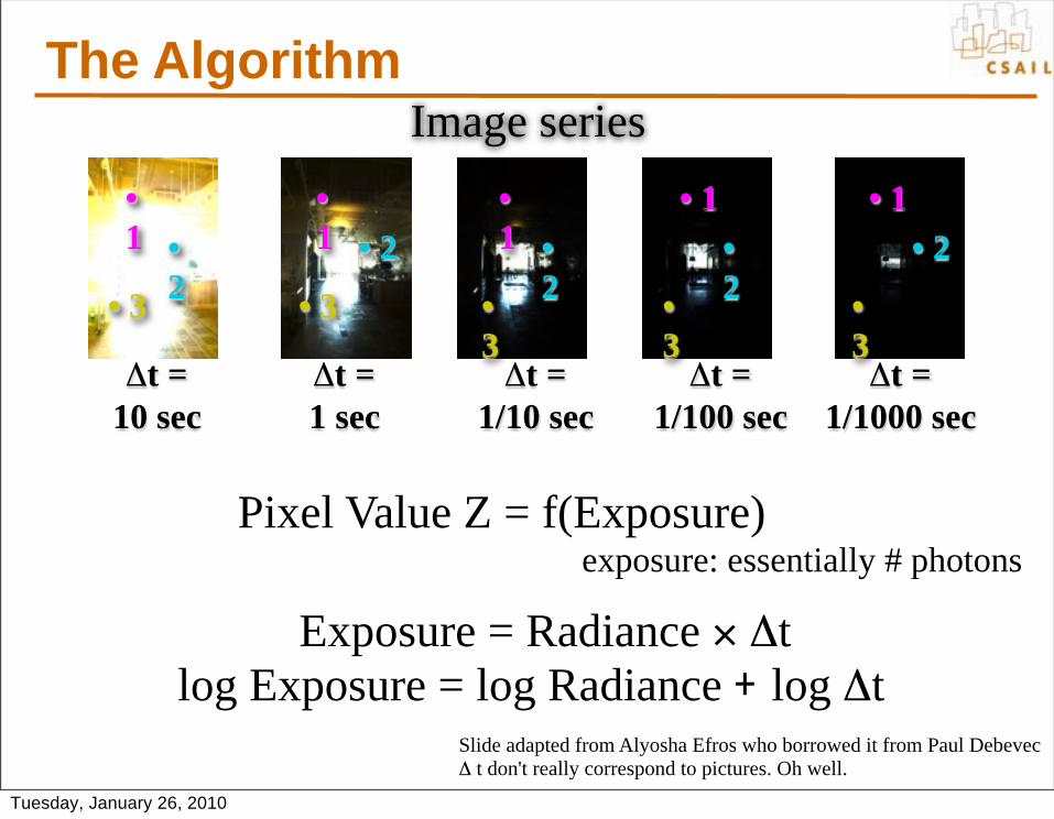
Image series
• 3
• 1 •
2
Δt =1/10 sec
Exposure = Radiance × Δtlog Exposure = log Radiance + log Δt
Pixel Value Z = f(Exposure)
Slide adapted from Alyosha Efros who borrowed it from Paul DebevecΔ t don't really correspond to pictures. Oh well.
The Algorithm
exposure: essentially # photons
Tuesday, January 26, 2010
log Exposure
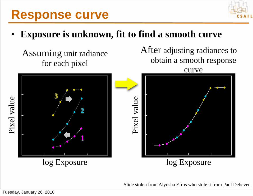
Assuming unit radiancefor each pixel
After adjusting radiances to obtain a smooth response
curve
Pixe
l val
ue
3
1
2
log Exposure
Pixe
l val
ue
Slide stolen from Alyosha Efros who stole it from Paul Debevec
Response curve• Exposure is unknown, fit to find a smooth curve
Tuesday, January 26, 2010
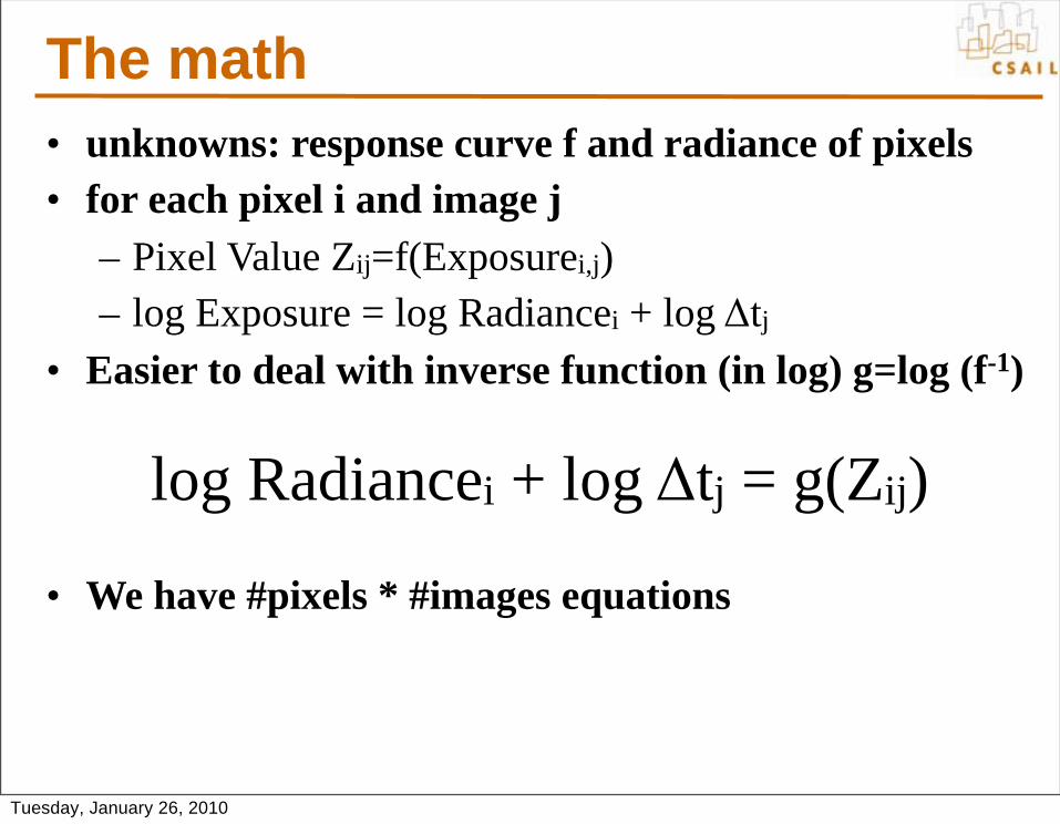
The math• unknowns: response curve f and radiance of pixels• for each pixel i and image j
– Pixel Value Zij=f(Exposurei,j)– log Exposure = log Radiancei + log Δtj
• Easier to deal with inverse function (in log) g=log (f-1)
• We have #pixels * #images equations
log Radiancei + log Δtj = g(Zij)
Tuesday, January 26, 2010
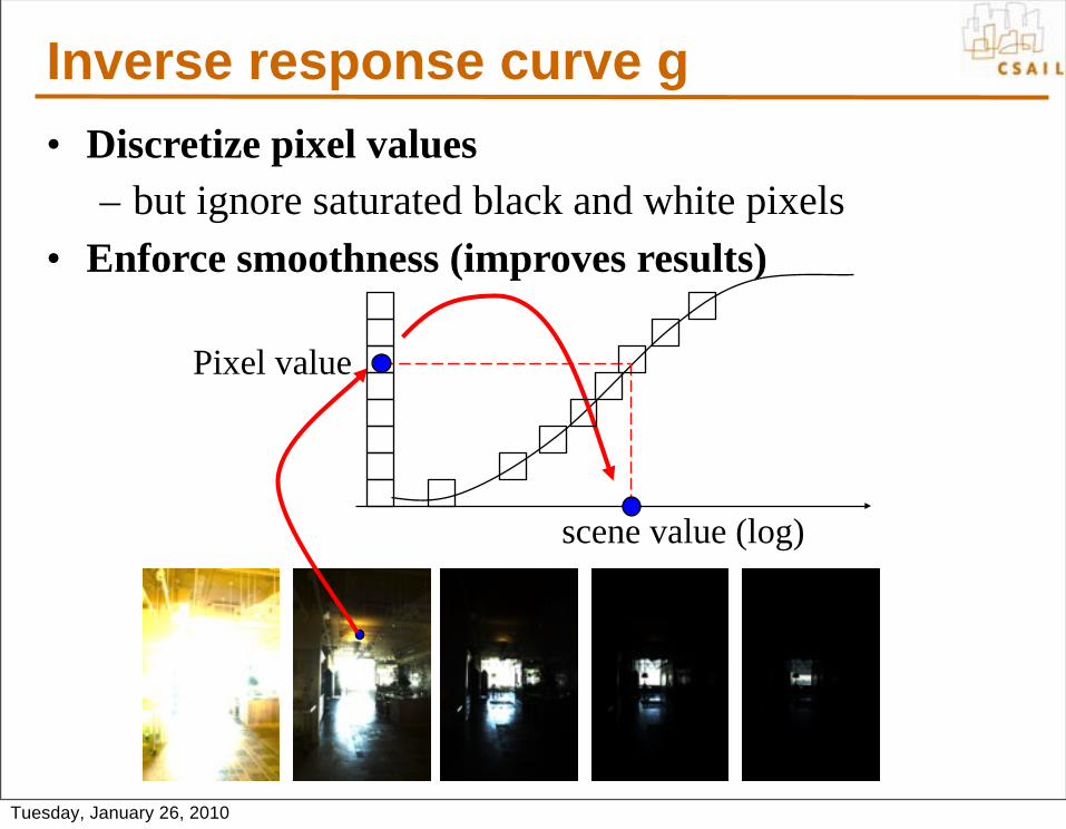
Inverse response curve g• Discretize pixel values
– but ignore saturated black and white pixels• Enforce smoothness (improves results)
Pixel value
scene value (log)
Tuesday, January 26, 2010
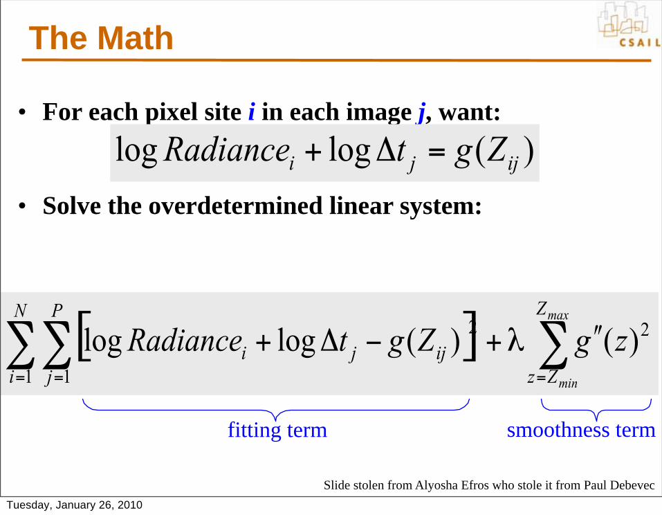
• For each pixel site i in each image j, want:
• Solve the overdetermined linear system:
fitting term smoothness term
Slide stolen from Alyosha Efros who stole it from Paul Debevec
The Math
Tuesday, January 26, 2010
Slide stolen from Alyosha Efros who stole it from Paul Debevec
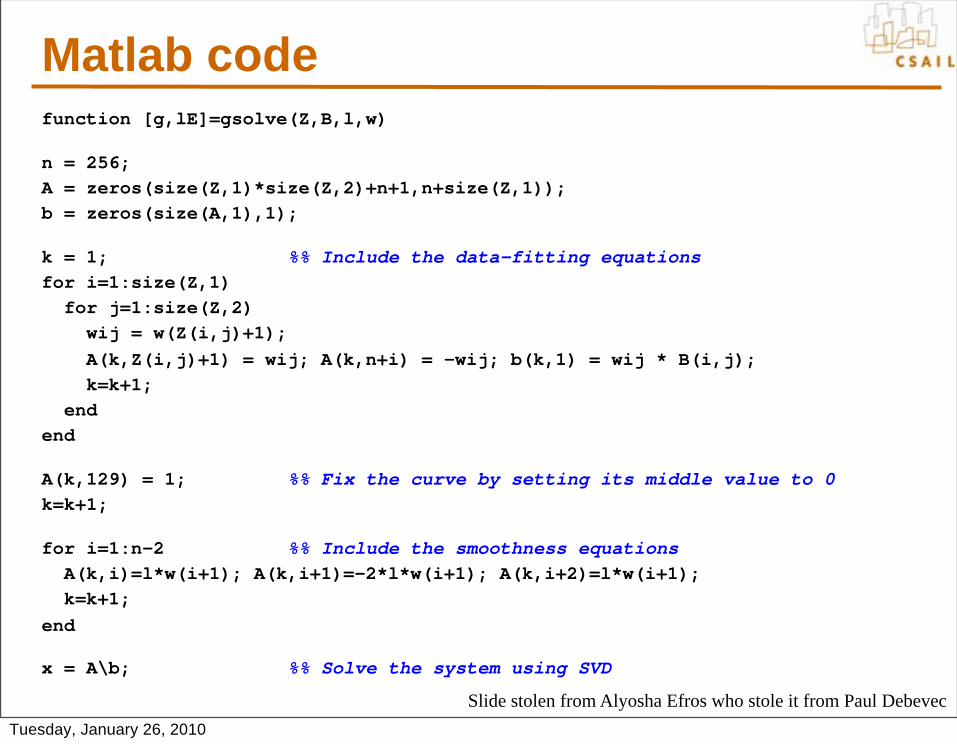
Matlab codefunction [g,lE]=gsolve(Z,B,l,w)
n = 256;A = zeros(size(Z,1)*size(Z,2)+n+1,n+size(Z,1));b = zeros(size(A,1),1);
k = 1; %% Include the data-fitting equationsfor i=1:size(Z,1) for j=1:size(Z,2) wij = w(Z(i,j)+1); A(k,Z(i,j)+1) = wij; A(k,n+i) = -wij; b(k,1) = wij * B(i,j); k=k+1; endend
A(k,129) = 1; %% Fix the curve by setting its middle value to 0k=k+1;
for i=1:n-2 %% Include the smoothness equations A(k,i)=l*w(i+1); A(k,i+1)=-2*l*w(i+1); A(k,i+2)=l*w(i+1); k=k+1;end
x = A\b; %% Solve the system using SVD
Tuesday, January 26, 2010
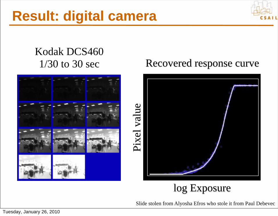
Recovered response curve
log Exposure
Pixe
l val
ue
Kodak DCS4601/30 to 30 sec
Slide stolen from Alyosha Efros who stole it from Paul Debevec
Result: digital camera
Tuesday, January 26, 2010
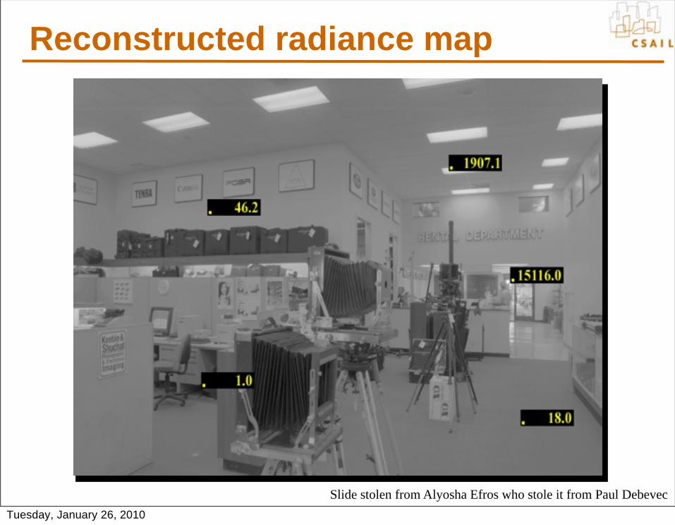
Slide stolen from Alyosha Efros who stole it from Paul Debevec
Reconstructed radiance map
Tuesday, January 26, 2010

• Kodak Gold ASA 100, PhotoCD
Slide stolen from Alyosha Efros who stole it from Paul Debevec
Result: color film
Tuesday, January 26, 2010
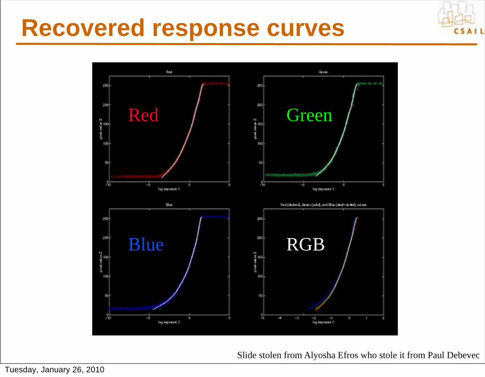
Red Green
RGBBlue
Slide stolen from Alyosha Efros who stole it from Paul Debevec
Recovered response curves
Tuesday, January 26, 2010

Recap• Curve calibration
– Take many images of static scene (1/3 stop)– Solve optimization problem
• HDR multiple-exposure merging– Take multiple exposures
(e.g. every 2 stops)– (optional) align images– for each pixel, use picture(s) where properly exposed
• use inverse response curve and exposure time– Output: one image where each pixel has full dynamic
range, stored e.g. in floataka radiance map
Tuesday, January 26, 2010
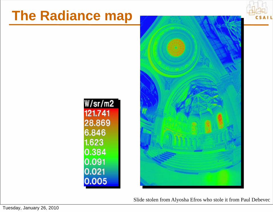
Slide stolen from Alyosha Efros who stole it from Paul Debevec
The Radiance map
Tuesday, January 26, 2010

Linearly scaled todisplay device
Slide stolen from Alyosha Efros who stole it from Paul Debevec
The Radiance map
Tuesday, January 26, 2010

Questions?
Tuesday, January 26, 2010
Today• Multiple-exposure High-Dynamic-Range imaging
• Tone mapping using the bilateral filter
Tuesday, January 26, 2010

Problem 2: Display the infromation• Match limited contrast of the medium• Preserve details
10-6 106
10-6 106
Real world
Picture
Low contrast
High dynamic range
Tuesday, January 26, 2010
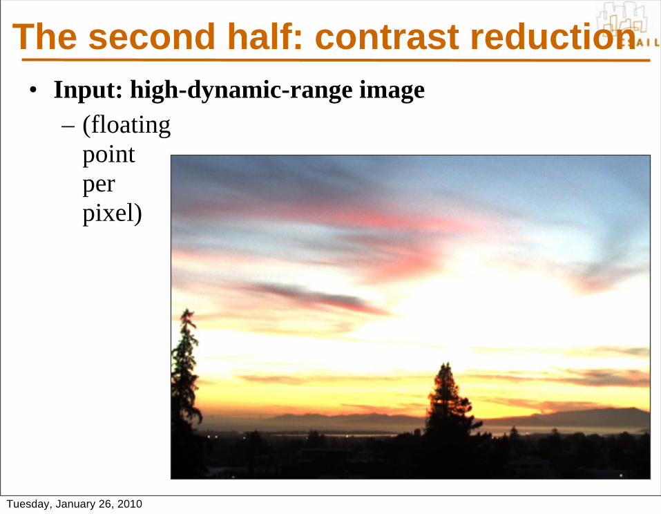
The second half: contrast reduction• Input: high-dynamic-range image
– (floating point per pixel)
Tuesday, January 26, 2010
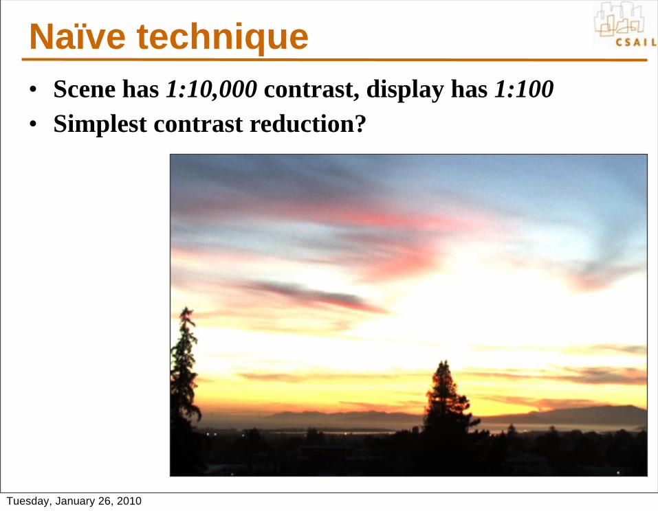
Naïve technique• Scene has 1:10,000 contrast, display has 1:100• Simplest contrast reduction?
Tuesday, January 26, 2010
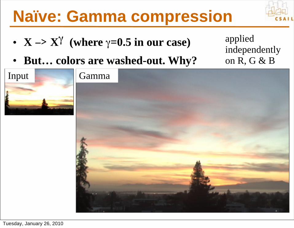
Naïve: Gamma compression• X −> Xγ (where γ=0.5 in our case)• But… colors are washed-out. Why?
Input Gamma
applied independently on R, G & B
Tuesday, January 26, 2010
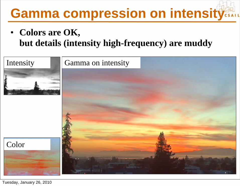
Gamma compression on intensity• Colors are OK,
but details (intensity high-frequency) are muddy
Gamma on intensityIntensity
Color
Tuesday, January 26, 2010
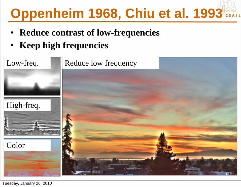
Oppenheim 1968, Chiu et al. 1993• Reduce contrast of low-frequencies• Keep high frequencies
Reduce low frequencyLow-freq.
High-freq.
Color
Tuesday, January 26, 2010
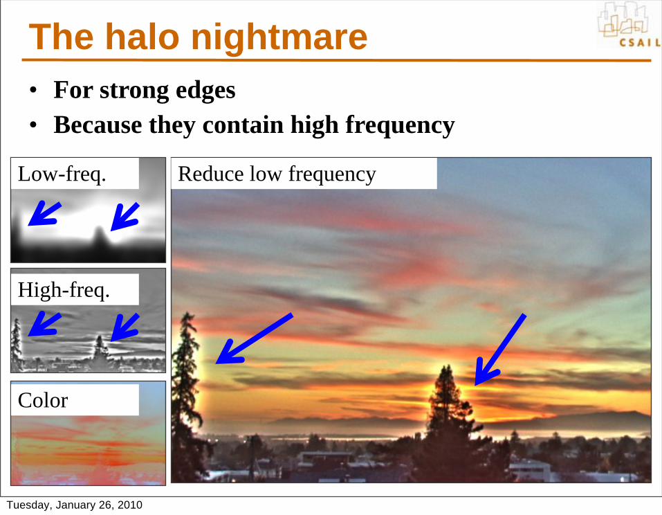
The halo nightmare• For strong edges• Because they contain high frequency
Reduce low frequencyLow-freq.
High-freq.
Color
Tuesday, January 26, 2010
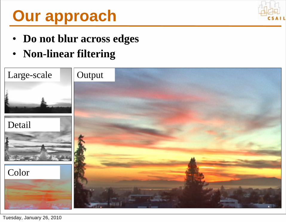
Our approach• Do not blur across edges• Non-linear filtering
OutputLarge-scale
Detail
Color
Tuesday, January 26, 2010

Bilateral filter• Tomasi and Manduci 1998]
– http://www.cse.ucsc.edu/~manduchi/Papers/ICCV98.pdf • Discussed for denoising in previous lecture• Related to
– SUSAN filter [Smith and Brady 95] http://citeseer.ist.psu.edu/smith95susan.html
– Digital-TV [Chan, Osher and Chen 2001]http://citeseer.ist.psu.edu/chan01digital.html
– sigma filter http://www.geogr.ku.dk/CHIPS/Manual/f187.htm
• Full survey: http://people.csail.mit.edu/sparis/publi/2009/fntcgv/Paris_09_Bilateral_filtering.pdf
Tuesday, January 26, 2010
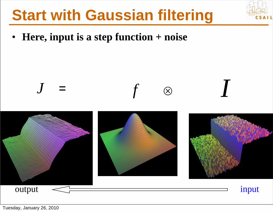
Start with Gaussian filtering• Here, input is a step function + noise
output input
€
J
€
=
€
f
€
⊗
€
I
Tuesday, January 26, 2010
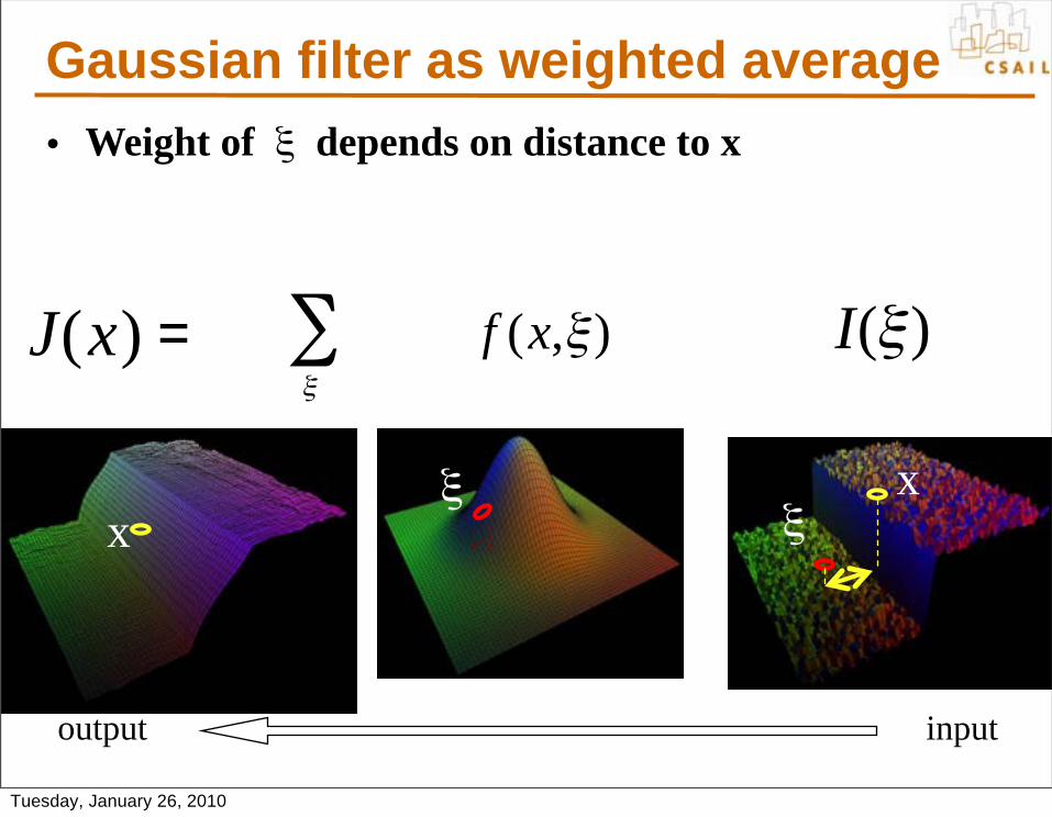
Gaussian filter as weighted average• Weight of ξ depends on distance to x
output input
€
ξ
∑
€
f (x,ξ)
€
I(ξ)
ξx
xξ
€
J(x)
€
=
Tuesday, January 26, 2010

The problem of edges• Here, “pollutes” our estimate J(x)• It is too different
output input
xξ
Ι(ξ)I(x)
Ι(ξ)
€
ξ
∑
€
f (x,ξ)
€
I(ξ)
€
J(x)
€
=
Tuesday, January 26, 2010
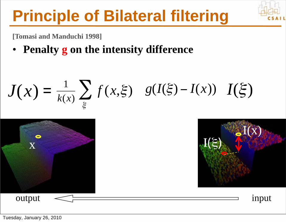
Principle of Bilateral filtering[Tomasi and Manduchi 1998]
• Penalty g on the intensity difference
output input
€
J(x)
€
=
€
1k(x)
€
ξ
∑
€
f (x,ξ)
€
g(I(ξ) − I(x))
€
I(ξ)
x Ι(ξ)I(x)
Tuesday, January 26, 2010
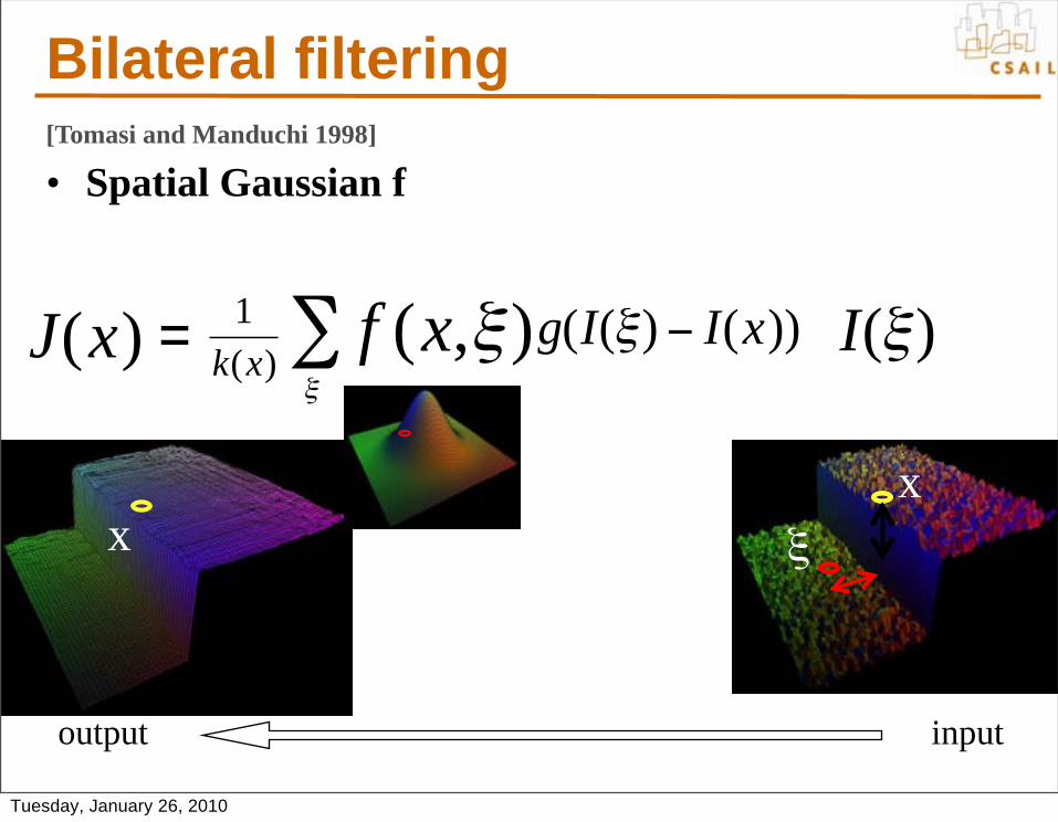
Bilateral filtering[Tomasi and Manduchi 1998]
• Spatial Gaussian f
output input
€
J(x)
€
=
€
1k(x)
€
ξ
∑
€
f (x,ξ)
€
g(I(ξ) − I(x))
€
I(ξ)
x ξx
Tuesday, January 26, 2010
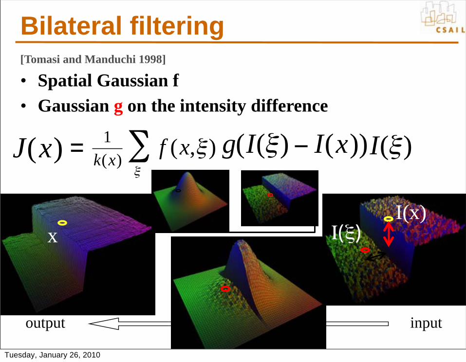
Bilateral filtering[Tomasi and Manduchi 1998]
• Spatial Gaussian f• Gaussian g on the intensity difference
output input
€
J(x)
€
=
€
1k(x)
€
ξ
∑
€
f (x,ξ)
€
g(I(ξ) − I(x))
€
I(ξ)
x Ι(ξ)I(x)
Tuesday, January 26, 2010
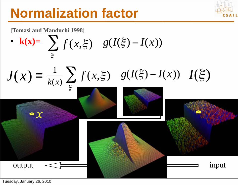
Normalization factor[Tomasi and Manduchi 1998]
• k(x)=
output input
€
J(x)
€
=
€
1k(x)
€
ξ
∑
€
f (x,ξ)
€
g(I(ξ) − I(x))
€
I(ξ)
€
ξ
∑
€
f (x,ξ)
€
g(I(ξ) − I(x))
Tuesday, January 26, 2010

Bilateral filtering is non-linear[Tomasi and Manduchi 1998]
• The weights are different for each output pixel
output input
Tuesday, January 26, 2010

Basic denoising
Noisy input Bilateral filter 7x7 window
Tuesday, January 26, 2010
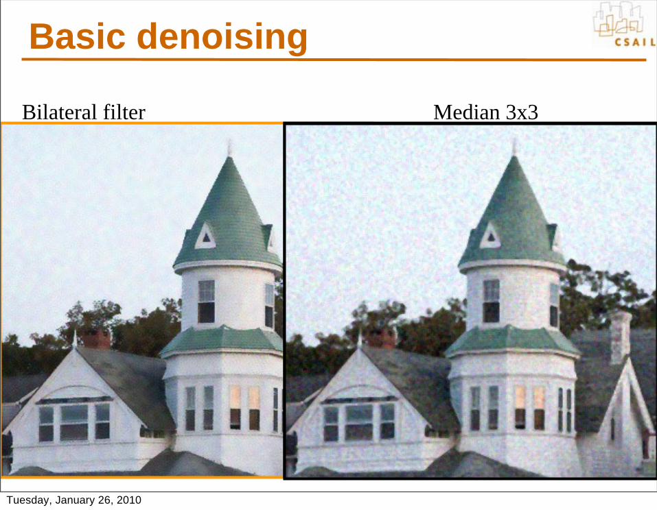
Bilateral filter
Basic denoising
Median 3x3
Tuesday, January 26, 2010

Bilateral filter
Basic denoising
Median 5x5
Tuesday, January 26, 2010

Basic denoising
Bilateral filter Bilateral filter – lower sigma
Tuesday, January 26, 2010
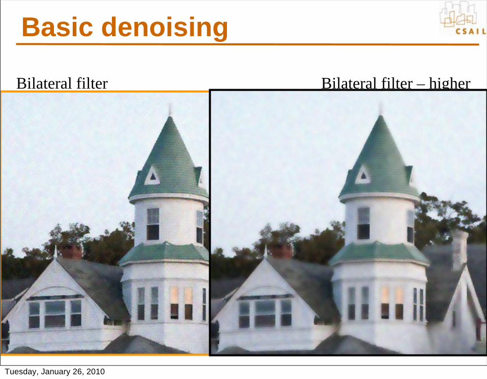
Bilateral filter
Basic denoising
Bilateral filter – higher sigma
Tuesday, January 26, 2010

Questions?
Tuesday, January 26, 2010

Questions?
Tuesday, January 26, 2010

Contrast reductionInput HDR image
Contrast too high!
Tuesday, January 26, 2010
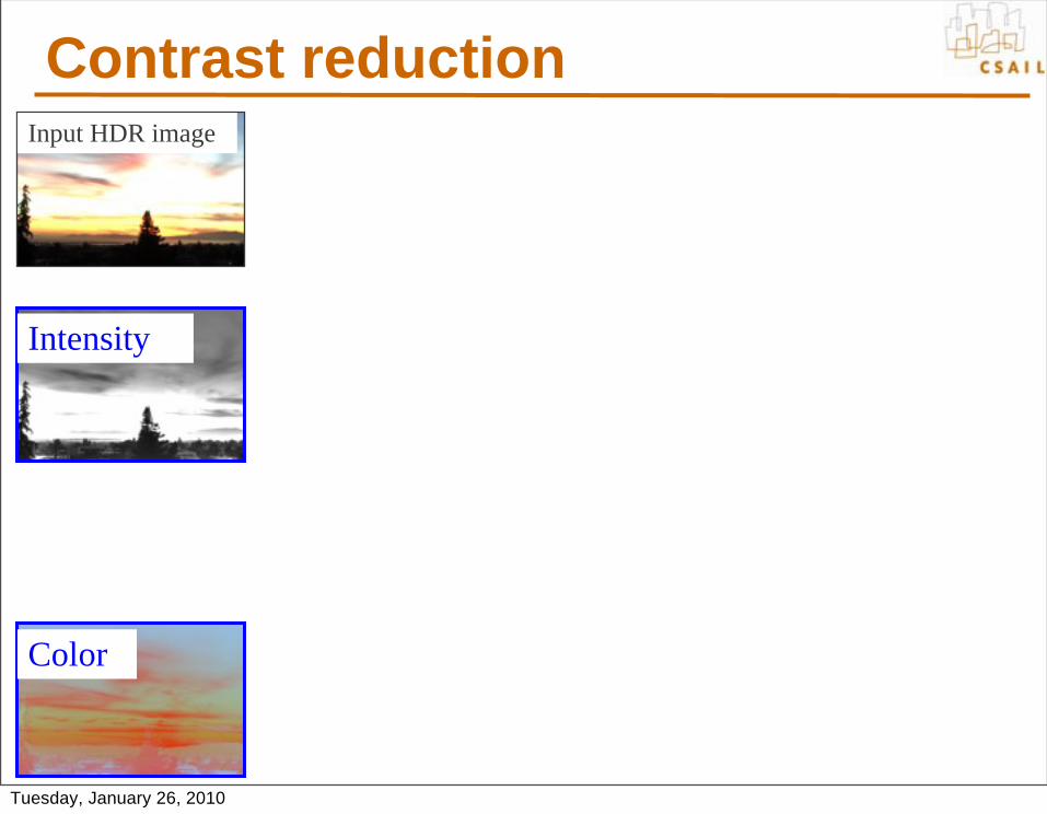
Contrast reduction
Color
Input HDR image
Intensity
Tuesday, January 26, 2010

Contrast reduction
Color
Intensity Large scale
Bilateral Filter
in log
Input HDR image
Spatial sigma: 2 to 5% image sizeRange sigma: 0.4 (in log 10)
Tuesday, January 26, 2010
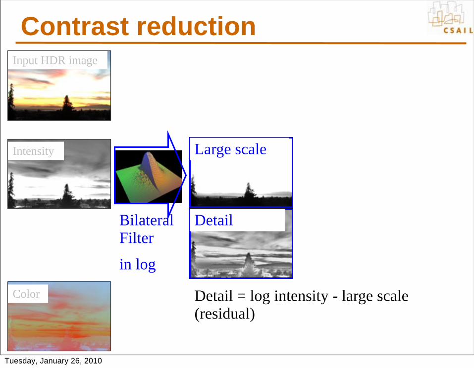
Contrast reduction
Detail
Color
Intensity Large scale
Bilateral Filter
in log
Input HDR image
Detail = log intensity - large scale(residual)
Tuesday, January 26, 2010
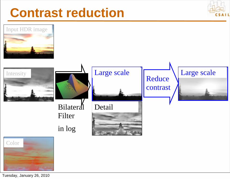
Contrast reduction
Detail
Color
Intensity Large scale
Bilateral Filter
in log
Reducecontrast
Large scale
Input HDR image
Tuesday, January 26, 2010

Contrast reduction
Detail
Color
Intensity Large scale
FastBilateral Filter
Reducecontrast
Detail
Large scale
Preserve!
Input HDR image
Tuesday, January 26, 2010

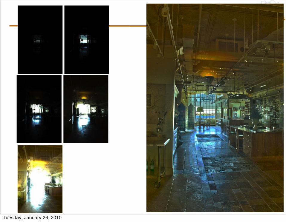
Contrast reduction
Detail
Color
Intensity Large scale
FastBilateral Filter
Reducecontrast
Detail
Large scale
Color
Preserve!
Input HDR image Output
Tuesday, January 26, 2010
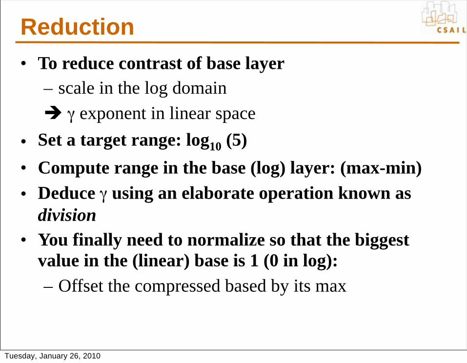
Reduction• To reduce contrast of base layer
– scale in the log domain γ exponent in linear space
• Set a target range: log10 (5)• Compute range in the base (log) layer: (max-min)• Deduce γ using an elaborate operation known as
division• You finally need to normalize so that the biggest
value in the (linear) base is 1 (0 in log):– Offset the compressed based by its max
Tuesday, January 26, 2010
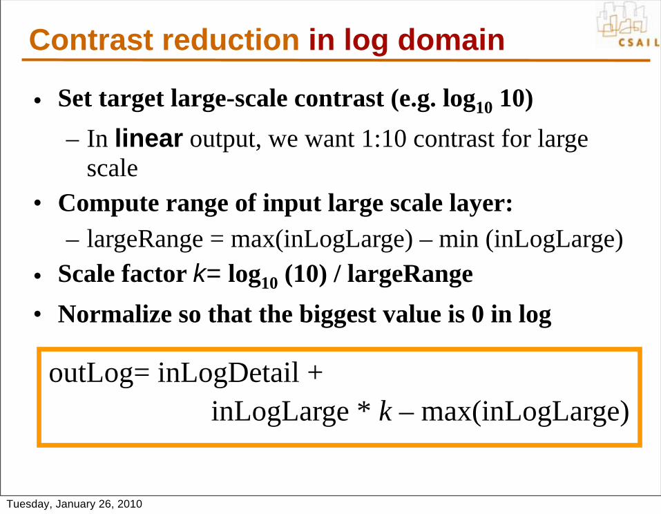
Contrast reduction in log domain
• Set target large-scale contrast (e.g. log10 10)– In linear output, we want 1:10 contrast for large
scale• Compute range of input large scale layer:
– largeRange = max(inLogLarge) – min (inLogLarge)• Scale factor k= log10 (10) / largeRange• Normalize so that the biggest value is 0 in log
outLog= inLogDetail + inLogLarge * k – max(inLogLarge)
Tuesday, January 26, 2010
Tuesday, January 26, 2010
What matters• Spatial sigma: not very important• Range sigma: quite important• Use of the log domain for range: critical
– Because HDR and because perception sensitive to multiplicative contrast
– CIELab might be better for other applications• Luminance computation
– Not critical, but has influence– see our Flash/no-flash paper [Eisemann 2004] for
smarter function
Tuesday, January 26, 2010
Speed• Direct bilateral filtering is slow (minutes)
• Fast algorithm: bilateral grid– http://groups.csail.mit.edu/graphics/bilagrid/– http://people.csail.mit.edu/sparis/publi/2009/ijcv/
Paris_09_Fast_Approximation.pdf– http://graphics.stanford.edu/papers/gkdtrees/
Tuesday, January 26, 2010

Tone mapping evaluation• User experiments to evaluate
competing tone mapping– Ledda et al. 2005 http://www.cs.bris.ac.uk/Publications/
Papers/2000255.pdf
– Kuang et al. 2004 http://www.cis.rit.edu/fairchild/PDFs/PRO22.pdf
• Interestingly, the former concludes bilateral is the worst, the latter that it is the best!– They choose to test a different criterion:
fidelity vs. preference
• More importantly, they focus on algorithm and ignore parameters
Adapted from Ledda et al.
From Kuang et al.
Tuesday, January 26, 2010
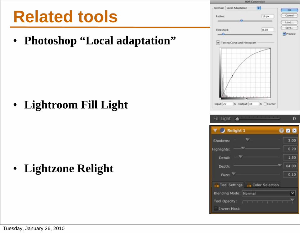
Related tools• Photoshop “Local adaptation”
• Lightroom Fill Light
• Lightzone Relight
Tuesday, January 26, 2010

Questions?
Tuesday, January 26, 2010
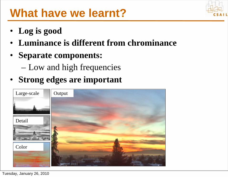
What have we learnt?• Log is good• Luminance is different from chrominance• Separate components:
– Low and high frequencies• Strong edges are important
OutputLarge-scale
Detail
Color
Tuesday, January 26, 2010
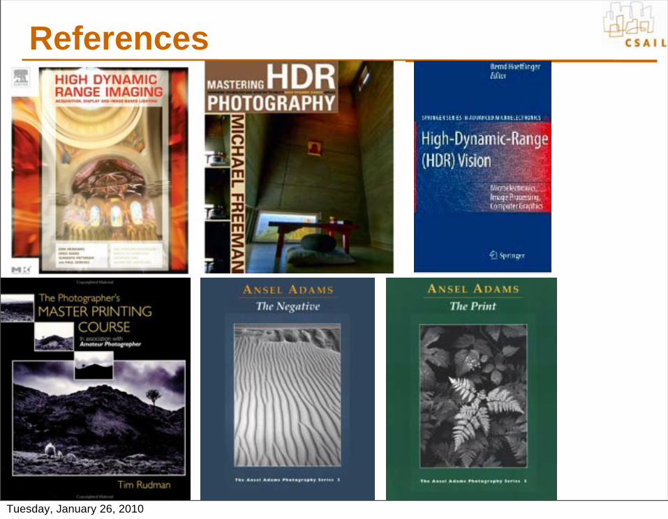
References
Tuesday, January 26, 2010
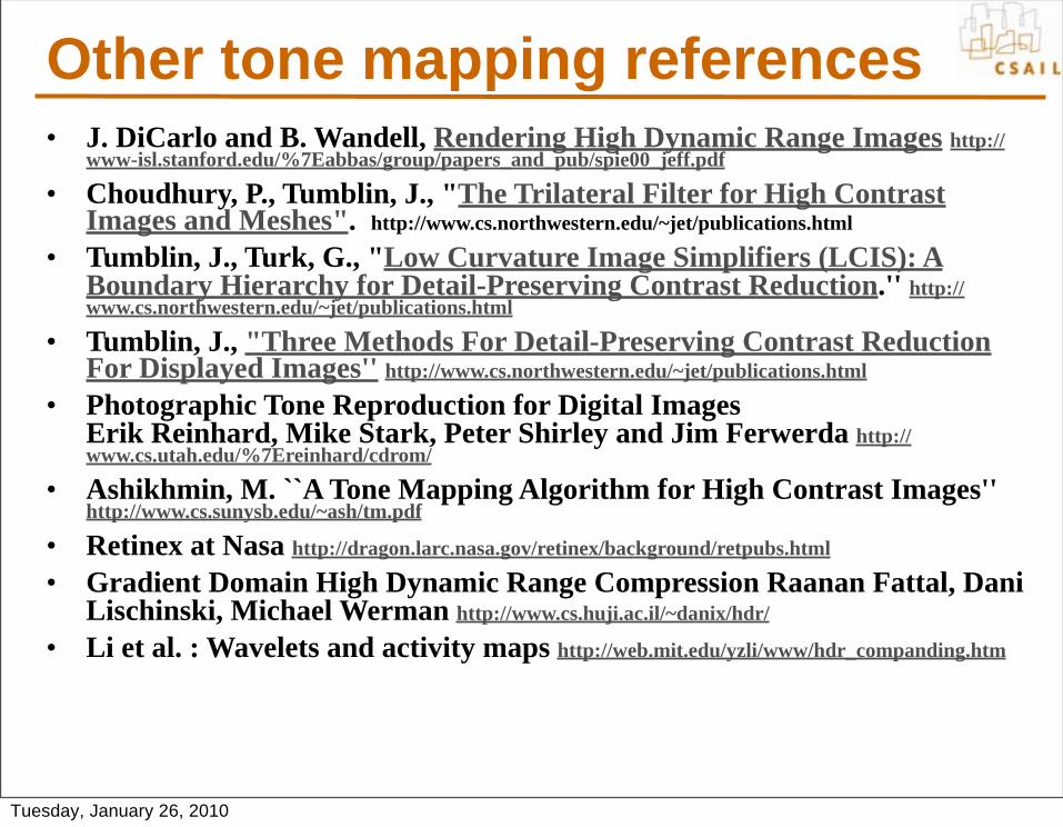
Other tone mapping references• J. DiCarlo and B. Wandell, Rendering High Dynamic Range Images http://
www-isl.stanford.edu/%7Eabbas/group/papers_and_pub/spie00_jeff.pdf
• Choudhury, P., Tumblin, J., "The Trilateral Filter for High Contrast Images and Meshes". http://www.cs.northwestern.edu/~jet/publications.html
• Tumblin, J., Turk, G., "Low Curvature Image Simplifiers (LCIS): A Boundary Hierarchy for Detail-Preserving Contrast Reduction.'' http://www.cs.northwestern.edu/~jet/publications.html
• Tumblin, J., "Three Methods For Detail-Preserving Contrast Reduction For Displayed Images'' http://www.cs.northwestern.edu/~jet/publications.html
• Photographic Tone Reproduction for Digital Images Erik Reinhard, Mike Stark, Peter Shirley and Jim Ferwerda http://www.cs.utah.edu/%7Ereinhard/cdrom/
• Ashikhmin, M. ``A Tone Mapping Algorithm for High Contrast Images'' http://www.cs.sunysb.edu/~ash/tm.pdf
• Retinex at Nasa http://dragon.larc.nasa.gov/retinex/background/retpubs.html
• Gradient Domain High Dynamic Range Compression Raanan Fattal, Dani Lischinski, Michael Werman http://www.cs.huji.ac.il/~danix/hdr/
• Li et al. : Wavelets and activity maps http://web.mit.edu/yzli/www/hdr_companding.htm
Tuesday, January 26, 2010
Tone mapping code• http://www.mpi-sb.mpg.de/resources/pfstools/• http://scanline.ca/exrtools/• http://www.cs.utah.edu/~reinhard/cdrom/source.html• http://www.cis.rit.edu/mcsl/icam/hdr/
•
Tuesday, January 26, 2010
Refshttp://people.csail.mit.edu/sparis/bf_course/http://people.csail.mit.edu/fredo/PUBLI/Siggraph2002/ http://www.hdrsoft.com/resources/dri.htmlhttp://www.clarkvision.com/imagedetail/dynamicrange2/http://www.debevec.org/HDRI2004/http://www.luminous-landscape.com/tutorials/hdr.shtmlhttp://www.anyhere.com/gward/hdrenc/http://www.debevec.org/IBL2001/NOTES/42-gward-cic98.pdf http://www.openexr.com/http://gl.ict.usc.edu/HDRShop/http://www.dpreview.com/learn/?/Glossary/Digital_Imaging/Dynamic_Range_01.htmhttp://www.normankoren.com/digital_tonality.htmlhttp://www.anyhere.com/ http://www.cybergrain.com/tech/hdr/
Tuesday, January 26, 2010
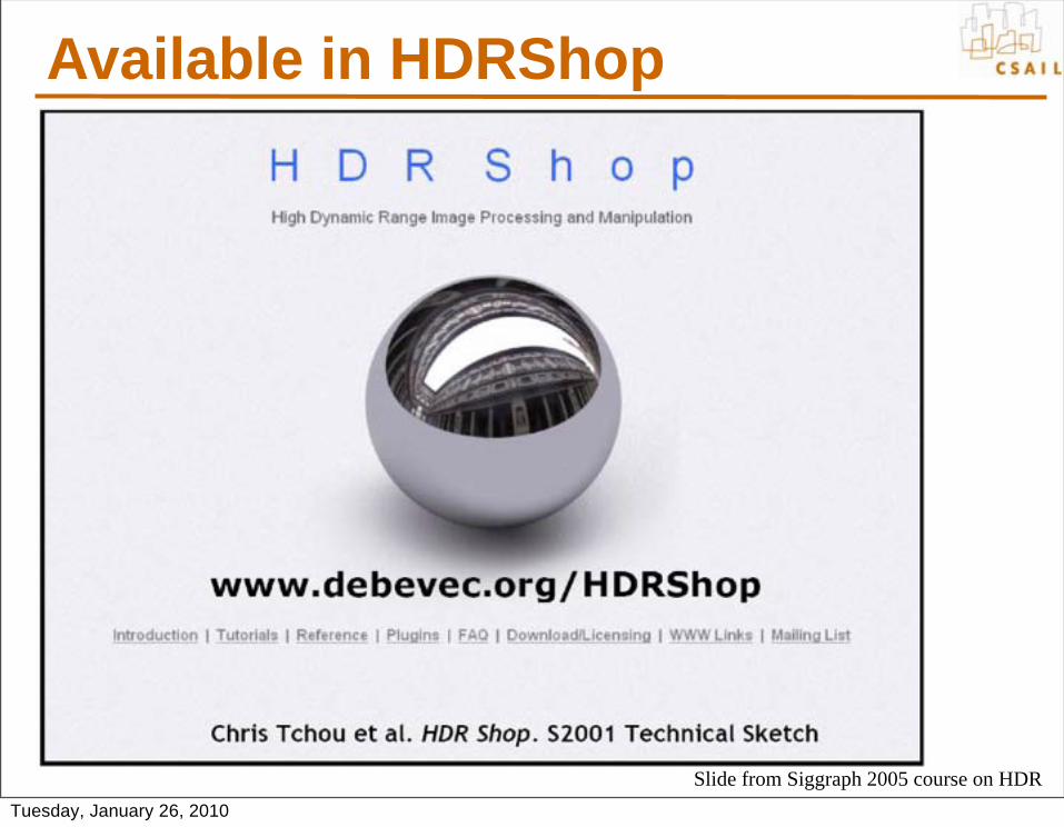
Available in HDRShop
Slide from Siggraph 2005 course on HDRTuesday, January 26, 2010
HDR combination papers• Steve Mann http://genesis.eecg.toronto.edu/wyckoff/
index.html• Paul Debevec http://www.debevec.org/Research/
HDR/• Mitsunaga, Nayar , Grossberg http://
www1.cs.columbia.edu/CAVE/projects/rad_cal/rad_cal.php
Tuesday, January 26, 2010

Questions?
Tuesday, January 26, 2010
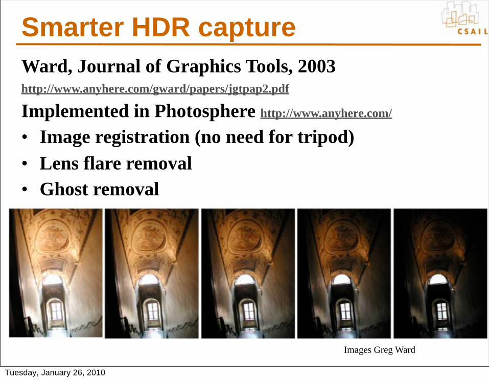
Smarter HDR captureWard, Journal of Graphics Tools, 2003http://www.anyhere.com/gward/papers/jgtpap2.pdf
Implemented in Photosphere http://www.anyhere.com/
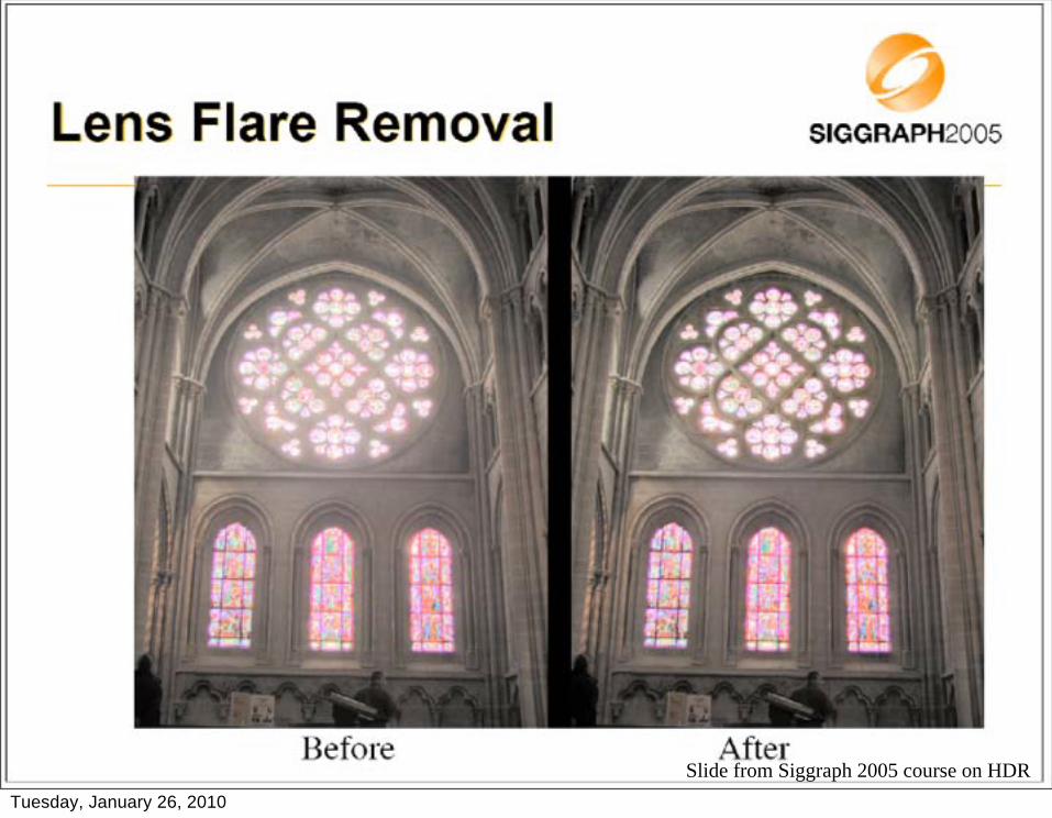
• Image registration (no need for tripod)• Lens flare removal• Ghost removal
Images Greg Ward
Tuesday, January 26, 2010

Image registration• How to robustly compare
images of different exposure? • Use a black and white version
of the image thresholded at the median– Median-Threshold Bitmap
(MTB)• Find the translation that
minimizes difference• Accelerate using pyramid
Tuesday, January 26, 2010
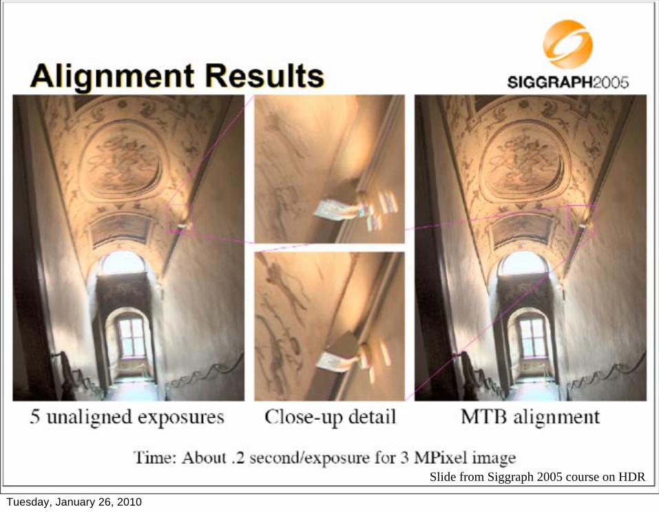
Slide from Siggraph 2005 course on HDR
Tuesday, January 26, 2010
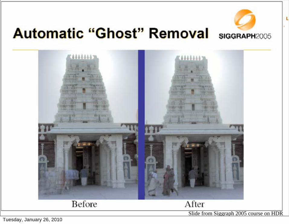
Slide from Siggraph 2005 course on HDRTuesday, January 26, 2010
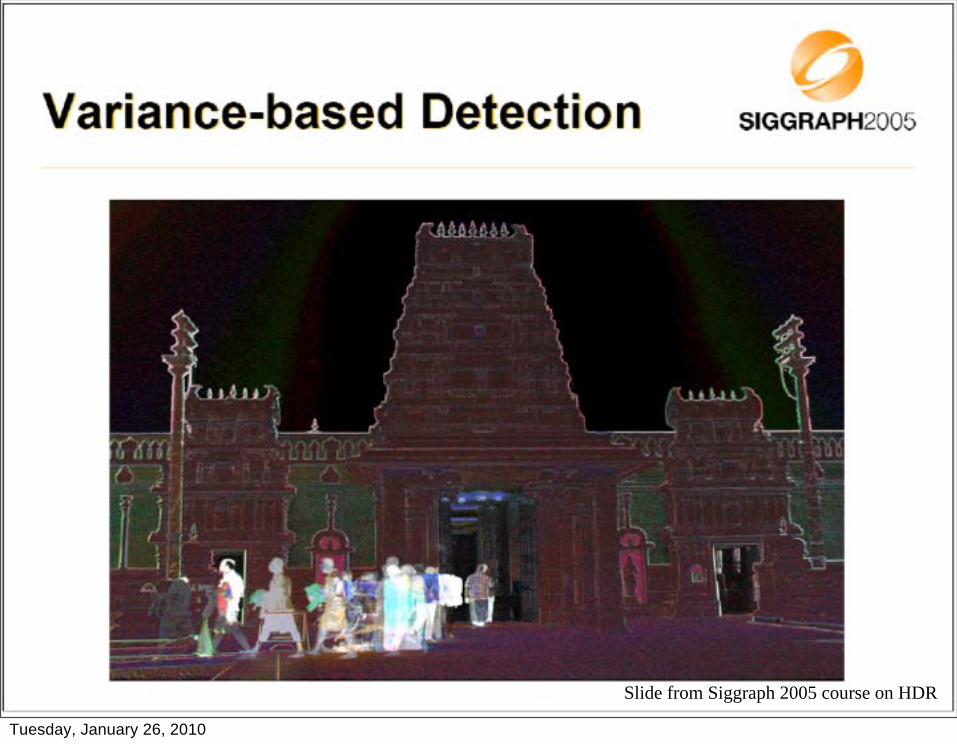
Slide from Siggraph 2005 course on HDR
Tuesday, January 26, 2010

Slide from Siggraph 2005 course on HDR
Tuesday, January 26, 2010

Slide from Siggraph 2005 course on HDR
Tuesday, January 26, 2010
Slide from Siggraph 2005 course on HDRTuesday, January 26, 2010
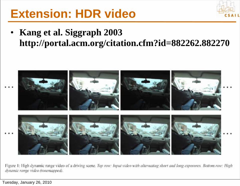
Extension: HDR video• Kang et al. Siggraph 2003
http://portal.acm.org/citation.cfm?id=882262.882270
Tuesday, January 26, 2010
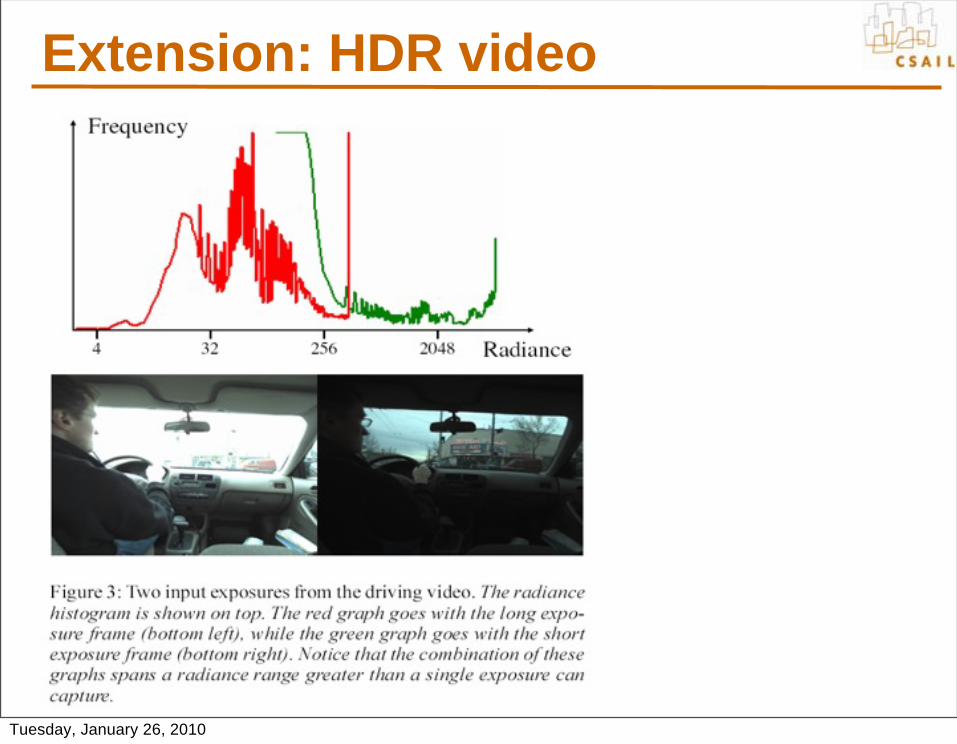
Extension: HDR video
Tuesday, January 26, 2010

Questions?
Tuesday, January 26, 2010

HDR encoding• Most formats are lossless• Adobe DNG (digital negative)
– Specific for RAW files, avoid proprietary formats• RGBE
– 24 bits/pixels as usual, plus 8 bit of common exponent– Introduced by Greg Ward for Radiance (light simulation)– Enormous dynamic range
• OpenEXR– By Industrial Light + Magic, also standard in graphics hardware– 16bit per channel (48 bits per pixel) 10 mantissa, sign, 5 exponent– Fine quantization (because 10 bit mantissa), only 9.6 orders of magnitude
• JPEG 2000– Has a 16 bit mode, lossy
Tuesday, January 26, 2010

HDR formats• Summary of all HDR encoding formats (Greg Ward):
http://www.anyhere.com/gward/hdrenc/hdr_encodings.html
• Greg’s notes: http://www.anyhere.com/gward/pickup/CIC13course.pdf
• http://www.openexr.com/ • High Dynamic Range Video Encoding (MPI) http://www.mpi-sb.mpg.de/resources/hdrvideo/
Tuesday, January 26, 2010
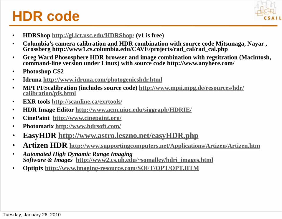
HDR code • HDRShop http://gl.ict.usc.edu/HDRShop/ (v1 is free)• Columbia’s camera calibration and HDR combination with source code Mitsunaga, Nayar ,
Grossberg http://www1.cs.columbia.edu/CAVE/projects/rad_cal/rad_cal.php• Greg Ward Phososphere HDR browser and image combination with regsitration (Macintosh,
command-line version under Linux) with source code http://www.anyhere.com/• Photoshop CS2• Idruna http://www.idruna.com/photogenicshdr.html• MPI PFScalibration (includes source code) http://www.mpii.mpg.de/resources/hdr/
calibration/pfs.html• EXR tools http://scanline.ca/exrtools/• HDR Image Editor http://www.acm.uiuc.edu/siggraph/HDRIE/• CinePaint http://www.cinepaint.org/ • Photomatix http://www.hdrsoft.com/ • EasyHDR http://www.astro.leszno.net/easyHDR.php• Artizen HDR http://www.supportingcomputers.net/Applications/Artizen/Artizen.htm• Automated High Dynamic Range Imaging
Software & Images http://www2.cs.uh.edu/~somalley/hdri_images.html• Optipix http://www.imaging-resource.com/SOFT/OPT/OPT.HTM
Tuesday, January 26, 2010
HDR images• http://www.debevec.org/Research/HDR/• http://www.mpi-sb.mpg.de/resources/hdr/gallery.html• http://people.csail.mit.edu/fredo/PUBLI/Siggraph2002/• http://www.openexr.com/samples.html• http://www.flickr.com/groups/hdr/ • http://www2.cs.uh.edu/~somalley/hdri_images.html#hdr_others• http://www.anyhere.com/gward/hdrenc/pages/originals.html• http://www.cis.rit.edu/mcsl/icam/hdr/rit_hdr/• http://www.cs.utah.edu/%7Ereinhard/cdrom/hdr.html• http://www.sachform.de/download_EN.html• http://lcavwww.epfl.ch/%7Elmeylan/HdrImages/February06/
February06.html• http://lcavwww.epfl.ch/%7Elmeylan/HdrImages/April04/april04.html• http://books.elsevier.com/companions/0125852630/hdri/html/images.html
Tuesday, January 26, 2010

HDR photography• http://luminous-landscape.com/essays/hdr-plea.shtml• http://en.wikipedia.org/wiki/
High_dynamic_range_imaging• http://www.cambridgeincolour.com/tutorials/high-
dynamic-range.htm• http://www.luminous-landscape.com/tutorials/
hdr.shtml•
Tuesday, January 26, 2010