health status and calorie inequalities linkage among major ... · health status and calorie...
TRANSCRIPT

Health Status and Calorie Inequalities Linkage among
Major Indian States: An Empirical Exploration
Amarjit Singh Sethi (Guru Nanak Dev University, India)
Ritu Pandhi (Shanti Devi Arya Mahilla College, Dinanagar, India)
Paper prepared for the 34
th IARIW General Conference
Dresden, Germany, August 21-27, 2016
PS1.5: Health
Time: Monday, August 22, 2016 [Late Afternoon]

Health Status and Calorie Inequalities Linkage among Major Indian States: An Empirical Exploration#
Amarjit Singh Sethi
1 and Ritu Pandhi
2
1Professor, Punjab School of Economics Guru Nanak Dev University, Amritsar (India) – 143 005
(E-mail: [email protected])
2Assistant Professor, Baring Union College, Batala (India) – 143531
(E-mail: [email protected])
Abstract
This paper aims at making an assessment of temporal shifts in relative positioning of the major Indian states, jointly
through the chief concomitants of health, as also through the measures of calorie inequalities. The task was
accomplished through factor analysis (with promax oblique rotation), duly coupled with canonical correlation
analysis, on the information on 16 indicators of health during three rounds for seventeen major Indian states. As per
the findings, major determinants of health status have undergone voluminous reshuffling during the study span.
Through composite index, states like Tamil Nadu, Maharashtra and Kerala were observed to have undergone
perceptible temporal improvements in health status, whereas the so-called better-off states like Punjab and Gujarat
have slipped fairly sharply in their relative rankings. As per FGT(2) index (due to Foster et al., 1984, 2010;
measuring relative deprivation), the averaged inequalities, within each of rural and urban regions, were highly
significantly different among the states as also among the rounds. Temporally, the inequalities portrayed an
inverted-U pattern. Gravity of the situation on calorie inequalities in south Indian states (like Tamil Nadu, Karnataka
and Kerala) was alarming whereas, on the other extreme, the same in certain north-Indian hilly states (like Himachal
Pradesh and Jammu & Kashmir) was manageable. Further, through panel data estimation, association between the
composite index of health status and FGT(2) measure of the inequalities was indirect and statistically significant.
There was a feeble indication of an indirect association between the measure of inequalities and per capita Income.
However, association between the composite index of health and per capita income was direct and very robust.
Thus, as a policy measure, there is a dire need for shifting priorities in favour of investment on both physical and
social health infrastructure, particularly in laggard states and in those states which have undergone a rapid slippage
in their ranking. Public-private-partnership model in this important social activity (which otherwise has remained a
soft target by the governments), may prove beneficial.
Key Words: Calorie Inequalities, Time Series Factor Analysis, Promax Oblique Rotation, Composite Index,
Canonical Correlation Analysis, FGT Index.
JEL Codes: C33, C38, I14, I15, R11, R58.
1. Introduction
As per WHO (1946), health of an individual is defined as a state of complete physical, mental
and social well being, and not merely absence of disease or infirmity. A community would be
healthy if a large majority of the individuals constituting the community are so. The basic
necessities for anyone to be healthy are availability of adequate amount of food (qualitative
———————————————————
# Accepted for the Presentation in the 34
th General Conference of the International Association for Research in
Income and Wealth (IARIW) to be held in Dresden, Germany (August 21-27, 2016).
enough so as to meet the bare minimal nutritional requirements), shelter and clothing which,
however, could be met only if there is a sufficient scope of income generation.
Health status of a cohort of people is characterized by a multiplicity of factors – demographic,
physical as well as social health infrastructure. Relative significance of these factors may differ
temporally as well as spatially. Furthermore, nutritional requirements necessary for keeping good
health are also known to vary across individuals and over time due to a multiplicity of reasons,
generally not known to us (Ravallion, 1992). In fact, an adequate nutritional intake by the
people is accepted as a meaningful yardstick for the success story of development policies of a
nation.
Among Indian states, there are known to exist wide inequalities in the level of development.
Although hunger and malnutrition are common, yet the extent and pattern differ from state-to-
state. Nutritional status of the population depends not merely on food production and availability
but more so on quantity and quality of food consumption. Uptil mid-sixties, nutritional problem
was considered as the one associated with protein deficiency, especially in respect of quality
protein from animal food. In line with the experience of a large majority of the developing
economies, nutritional levels of the people are inadequate.
This paper aims at making an assessment of temporal shifts in relative positioning of the major
Indian states, jointly through the chief concomitants of health, as also through the measures of
calorie inequalities. An evaluation has also made on the relative positioning of the states, jointly
on the basis of the so-identified determinants, so as to enable policy-makers to adopt policies
conducive for balanced growth.
The paper has been organized into six sections in all, including the current one. The second
section deals with a brief review of the related literature, so as to assist us in having a feel of the
research gaps, if any, which possibly could be filled through the present study. A brief mention
of the data base has been made in the third section, whereas analytical techniques adopted in the
study have been mentioned in the fourth section. The fifth section is devoted to a brief discussion
on the results obtained, first on health issues and then on calories inequalities. And, finally,
concluding remarks and policy implications have been given in the sixth section.
2. Literature Reviewed
In the Indian context and elsewhere, a large number of empirical studies have been carried out on
temporal and interregional status of health and nutrition, some of which have been reviewed in
this section. As per Sukhatme (1970), calorie deficiency was of grave concern; in almost all
classes of people, there was no group that was protein deficient, but no group that was not calorie
deficient. His findings were duly supported by Gopalan (1970), Gopalan et al., (1971) for India,
and by Ghassemi (1972) for Iran. Subsequently, malnutrition caused by calorie deficiency
assumed the central concern, especially among economists who took it as a basis for their
measurement of poverty. In their pioneering study, Dandekar and Rath (1971) estimated poverty
line on the basis of minimum calorie requirement, and magnitude of the proportion of people
living below this level was considered as measurement of poverty. In order to examine the trends
in inter-regional and inter-sectoral disparities in India, Rao (1971) constructed a composite
index, and observed that less developed states were moving towards national composite rate and
that the inter-state disparities were reducing. However, Rao (1973) opined that disparities had
not come down at the pace as these should have been in the course of 15 years of planning.
Bardhan (1974a, 1974b) and Srinivasan (1974) have contributed significantly towards
distributional aspects of income and poverty in India. Chatterjee and Bhattacharya (1974) found
that a glaring 60 percent of the real population was below the all India average intake in respect
of calorie and all other nutrients, except vitamin C for which the proportion was 40 percent.
Expressing his views on ‘Some Nutritional Puzzles’, Rao (1981) emphasised on balanced diet
that would secure both the energy intake and the nutrients needed for good health. He suggested
that the first step required for formulating a nutritional policy on food and nutrition is to
formulate calorie intake norms that could be unambiguously used for estimating food
requirements and, therefore, the deficits that have to be made up by increasing overall supplies.
Dasgupta (1983) examined the intake of different nutrients for people of different age-sex-
activity group. However, the study made no mention of the extent of inequality in nutritional
intake. Dasgupta (1984) further studied the average intake of calories and proteins in India.
Making use of the inequality indices G1, G2, and index of under-nutrition U, he found that
although nutritional inequality was more evident in rural areas, the problem was not only of
distribution but also of availability itself. In his analysis on inter-linkages between regional
imbalances and plan outlays for 15 Indian states, Sarkar (1994) observed that Punjab scored the

highest and Bihar the lowest rank on the level of development. Through the construction of a
composite index, Pathak and Gaur (1997) tried to find out in relative terms, the health status of
different states in India. As per their findings, life expectancy at birth is an indicator of
improvement, whereas each of infant mortality rate and crude birth rate are the indicators of
deterioration in the health status of the Indian states. Emphasizing on the need to focus on the
expansion of human capabilities, Das (1999) observed that the factors like education, availability
of food, minimum purchasing power, facilities like safe drinking water, health infrastructure,
etc., played an important role in development process. Rao (2000) measured the effects of major
forces affecting consumption of pulses during two periods of time, viz., 1961 and 1971, in rural
areas of two districts of Delhi. The author found that the income effect of pulses changed from
positive to negative, indicating a rise in the general standard of living. Rao also observed a shift
from consumption of energy food to consumption of body building and protective foods. Au et
al. (2001) examined regional variations in the physical and mental health of patients receiving
primary care in the largest integrated health care system in the United States. As per their
findings, substantial differences in the health of patients enrolled in different VA primary clinics
could be attributed to socio-demographic and co-morbid factors. Sethi (2003) emphasized that
social sector strengthening (through increased government expenditure on health and education)
would expectedly reduce the incidence of poverty via providing more employment opportunities,
bringing down the death rate, and increasing the literacy rate. He stressed that reducing
disparities and structural imbalances of the economy could be a long-lasting solution to bringing
down the incidence of poverty. Roy et al. (2004) made an assessment of the extent of inequalities
in health care and nutritional status across the Indian states with a focus on caste and tribe, and
concluded that health services did not reach the disadvantaged sections. Kathuria and Sankar
(2005) analyzed the performance of the rural public health systems of 16 major states in India,
using stochastic production frontier techniques and panel data for the period 1986–97. The
authors found that the health outcomes of Indian states in rural areas were positively related to
the level of health infrastructure in terms of access to facilities and availability of skilled
professionals, such as doctors. Their results further showed that states differed, not only in
capacity building in terms of health infrastructure created but also in efficiency in using these
inputs. Nair (2007) analyzed inter-state differentials in malnourishment among children in India
on the basis of National Family Health Surveys: 1992–93, 1998–99, and 2005–6. The study
brought out the prevalence of widespread disparities and indicated that differentials were
increasing over time. Such differentials, according to the author, did not always vary with the
extent of poverty gaps among the states. Gupta (2009) made an inter-state comparison with
respect to economic well-being, health, education, human development index, status of women,
and social opportunities, and observed the presence of a strong relationship between these
variables. Kumar (2011) noticed that wide regional disparities in women’s status were present
across states, which have persisted over time with little change in the development ranking of the
Indian states. Punjab, Haryana, Kerala, Gujarat and Tamil Nadu have continued to occupy higher
ranks in the index of economic development over time, while states like Bihar, Madhaya
Pradesh, Rajasthan and Uttar Pradesh have lagged behind. Kumari (2011) measured inter-district
disparity in education and health attainment in Uttar Pradesh state at two points in time: 1990-91
and 2007-08. Through principal component analysis, her results revealed that apart from the
presence of wide disparities, there were some regions/ districts that have performed well in
educational attainment, but are poorly placed in terms of health attainment and vice-versa.
Certain other studies (such as, due to Datta & Ganguly, 2002; Randhawa & Chahal, 2005; Giri,
2006; Musebe & Kumar, 2006; Nasurudeen et al. 2006; Chadha, 2007; Mittal, 2007; Kumar et
al., 2007; etc.) have analyzed the dynamics of per capita expenditure on various food groups
across different income groups and arrived at the general conclusion that the share of non-cereal
items in monthly per capita expenditure has consistently increased over time in both rural and
urban regions. Sethi and Pandhi (2011a, 2011b) observed that a major chunk of consumption
expenditure in India was incurred on items like Milk & Milk Products and Cereals, whereas the
least expenditure was allocated to Fruits & Nuts and Spices. Through the application of Fisher’s
linear discriminant analysis, the authors detected the prevalence of voluminous interstate
divergences in per capita consumption expenditure on major food items. Sethi and Pandhi
(2012a, 2013) estimated the extent of inequalities in calorie intake among the Indian states/
union territories (UTs), and also identified the chief determinants of the inequalities. In another
empirical study, Sethi and Pandhi (2012b) observed (through the applications of MANOVA and
clustering techniques) the presence of high-profile gaps among states and UTs with respect to per
capita per diem intake of calories, protein, and fat, separately for rural and urban regions.
Further, Sethi and Pandhi (2014) examined the extent of interstate divergences (through a more
robust general classificatory analysis) with respect to consumption expenditure on major food
items in India, and also to identify the clusters of the states at a similar level of the expenditure.
The present study was a step further, wherein we have made an attempt to seek knowledge on the
extent of interlinkage between health and nutritional aspects among the Indian states which, in
turn, is expected to provide with a useful input for appropriate policy formulation at the regional
level.
3. Data
For the purpose of identification of the major determinants of health, numerical information was
compiled on as many as 16 indicators of health at three points in time: 1999-00, 2004-05, and
2011-12. The points had a close proximity with three Rounds of National Sample Surveys
Organisation (NSSO) on Nutritional Intake in India: 55th
(July, 1999 - June, 2000), 61st (July,
2004 - June, 2005) and 68th
(July, 2011 - June, 2012). The indicators considered in the study
were a mixture of demographic (or endogenous) variables [viz., Birth Rate (BRRT, per 1000
population p.a.), Death Rate (DTRT, per 1000 population p.a.), Infant Mortality Rate (IMRT, per
1000 live births p.a.), and Life Expectancy at Birth (LEBR, in years)]; exogenous variables on
physical and social infrastructure of health [viz., Number of Hospitals per 100 Sq Km (NHPK),
Number of Hospital Beds per Lakh of Population (NBPL), Number of Sub-Centers per 100 Sq
Km (SBPK), Number of Primary Health Centers per 100 Sq Km (PHPK), Number of
Community Health Centers per 100 Sq Km (CHPK), Number of Doctors per Lakh of Population
(DCPL), Number of Pharmacists per Lakh of Population (PRPL), Number of Auxiliary Nursing
Midwives per Lakh of Population (ANPL), Number of Lady Health Visitors per Lakh of
Population (LVPL), Number of Nurses per Doctor (NRPD), and Number of Assistants per
Doctor (NAPD)]; and level of living [viz. Per Capita Income (PCIN, in Rs’000)]. The major
seventeen Indian states considered in the study were: Andhra Pradesh (ANP), Assam (ASM),
Bihar (BHR), Gujarat (GUJ), Haryana (HAR), Himachal Pradesh (HMP), Jammu and Kashmir
(JNK), Kerala (KRL), Karnataka (KTK), Madhya Pradesh (MDP), Maharashtra (MHR), Orissa
(ORS), Punjab (PNB), Rajasthan (RAJ), Tamil Nadu (TND), Uttar Pradesh (UTP), West Bengal
(WBN).
For measuring calorie inequalities among the states, data on the distribution of households by
calorie intake level for different MPCE (i.e., Monthly Per Capita Expenditure) classes of each of
the states under study (separately for rural and urban regions), were culled out from the Reports
of 55th
, 61st and 68
th Rounds of NSSO on Nutritional Intake in India. As has been mentioned in
Sethi and Pandhi (2012a), the data provides the two-way distribution of persons by calorie intake
level. For constructing these tables, NSSO has used the information on per 1000 distribution of
households by MPCE classes and by class intervals of actual calorie intake level as percent of
normative level of 2700 kcal, for both rural and urban areas.
4. Analytical Techniques
For accomplishing the task, we have made use of analytical techniques, like canonical
correlation analysis and exploratory factor analysis, duly followed by FGT(2) measure of
nutritional inequalities. As per requirements of the former two multivariate analytical techniques,
each of the manifest variables were considered in comparable terms (either in terms of per unit
population or in terms of per unit area) and were suitably re-expressed, if required, in such a
manner that higher value of each of the variables indicated towards better health status of a state.
For instance, Death Rate was transformed into 1000/DTRT. Similar was the treatment in respect
of Birth Rate and Infant Mortality Rate. Before subjecting the transformed data to the analysis,
each of the variables were duly standardized for their mean (μ) and standard deviation ().
4.1. Canonical Correlation Analysis
Canonical correlation analysis, introduced originally by Hotelling way back in 1935, is known to
be a very versatile multivariate technique for identifying relationships between two groups of
variables. The analysis aims primarily at studying overall association between linear composites
(called canonical variates) between two multivariate data sets (Akbas and Takma, 2005;
Menderes et al., 2005). Intrinsically, the analysis aims at identifying the optimum structure or
dimensionality of each variable set that maximizes the relationships between the two sets of
variables. An added advantage of the canonical correlation analysis is that it places the minimal
restrictions on the types of data on which it operates.
Let there be p variates in Group-1 (say, endogenous variables of health) and q variates in Group-
2 (say, endogenous variables of health), so that p q. Let the variates in the two groups be X1,
X2, …, Xp and Y1, Y2, …, Yq , respectively. Suppose we write down the matrix of inter-
correlation coefficients between the variables as
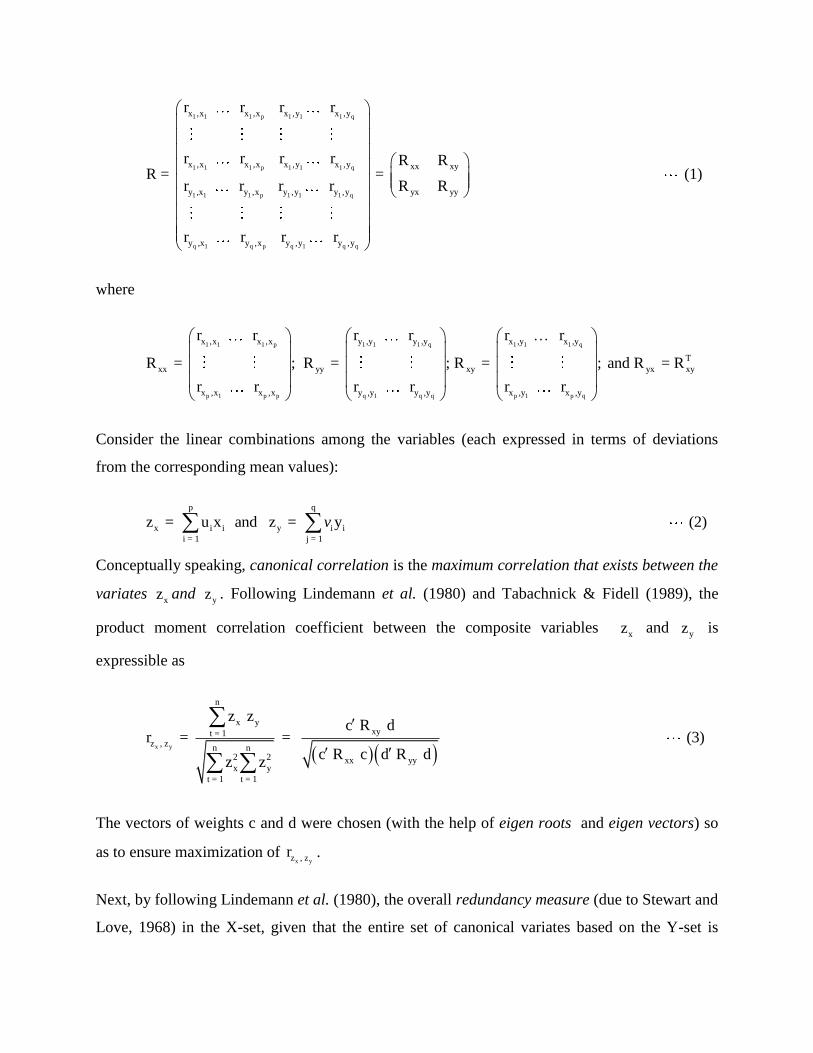
1 1 1 p 1 1 1 q
1 1 1 p 1 1 1 q
1 1 1 p 1 1 1 q
q 1 q p q
x ,x x ,x x ,y x ,y
x ,x x ,x x ,y x ,y
y ,x y ,x y ,y y ,y
y ,x y ,x y ,y
r r r r
r r r rR =
r r r r
r r r1 q q
xx xy
yx yy
y ,y
R R = (1)
R R
r
where
1 1 1 p 1 1 1 q 1 1 1 q
p 1 p p q 1 q q p 1 p q
x ,x x ,x y ,y y ,y x ,y x ,y
xx yy xy yx
x ,x x ,x y ,y y ,y x ,y x ,y
r r r r r r
R = ; R = ; R = ; and R
r r r r r r
T
xy = R
Consider the linear combinations among the variables (each expressed in terms of deviations
from the corresponding mean values):
p q
x i i y i i
i = 1 j = 1
z = u x and z = y (2) v
Conceptually speaking, canonical correlation is the maximum correlation that exists between the
variates xz and
yz . Following Lindemann et al. (1980) and Tabachnick & Fidell (1989), the
product moment correlation coefficient between the composite variables xz
and
yz is
expressible as
x y
n
x yxyt = 1
z , zn n
2 2 xx yyx y
t = 1 t = 1
z zc R d
r = = (3) c R c d R d
z z
The vectors of weights c and d were chosen (with the help of eigen roots and eigen vectors) so
as to ensure maximization of x yz , zr .
Next, by following Lindemann et al. (1980), the overall redundancy measure (due to Stewart and
Love, 1968) in the X-set, given that the entire set of canonical variates based on the Y-set is

available, was computed. The redundancy measure in the Y-set, given that the entire set of
canonical variates based on the X-set is available, was computed similarly. (Computational steps
for the measures are given in details in Sethi and Kumar, 2013).
4.2. Exploratory Factor Analysis
In order to accomplish the twin objectives of (a) making an assessment of temporal shifts in
relative positioning of the major Indian states, jointly through the chief concomitants of health,
and (b) making an evaluation of the relative positioning of the states, jointly on the basis of the
so-identified determinants, we have made use of exploratory factor analysis approach. This
dimensionality-reduction statistical technique aimed at disclosing latent traits, called factors,
which presumably underlie a regions’ performance on the given set of observed variables and
explain their interrelationships. These factors are not directly measurable, but are instead latent
or hidden random variables or constructs, with the observed measures being their indicators or
manifestations in overt behavior (Raykov and Markoulides, 2008). One of the major objectives
of Factor Analysis (FA) was to explain the pattern of the manifest (observable) variable
interrelationships with as few (latent) factors as possible. Thereby, the factors are expected to be
substantively interpretable and to explain why certain sets (or subsets) of observed variables are
highly correlated among themselves. More specifically, the aims of FA could be summarized as:
(i) to determine if a smaller set of factors could explain the interrelationships among a number of
original variables; (ii) to find out the number of these factors; (iii) to interpret the factors in
subject-matter terms; and (d) to provide estimates of their individual factor scores, so as
construct composite index for evaluating relative performance of the major Indian states.
As regards the underlying model in factor analysis technique, let us denote a column vector of p
observed variables by 1 1 px = (x , x ,..., x ) , wherein each of the variables were standardised (in the
usual way for their mean and standard deviation) beforehand so that each had a zero mean and
unit variance. The FA model is then put as:
1 11 1 12 2 1m m 1
2 21 1 22 2 2m m 2
p p1 1 p2 2
x = λ F + λ F + + λ F + ε
x = λ F + λ F + + λ F + ε
... (4)
x = λ F + λ F + pm m p + λ F + ε
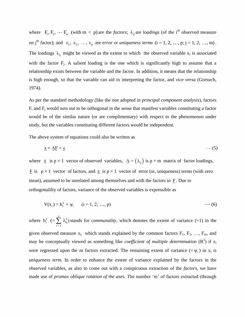
where 1 2 mF , F , F (with m < p) are the factors; ijλ are loadings (of the i
th observed measure
on jth
factor); and 1 2 pε , ε , , ε are error or uniqueness terms (i = 1, 2, , p; j = 1, 2, , m) .
The loadings ijλ might be viewed as the extent to which the observed variable xi is associated
with the factor Fj. A salient loading is the one which is significantly high to assume that a
relationship exists between the variable and the factor. In addition, it means that the relationship
is high enough, so that the variable can aid in interpreting the factor, and vice versa (Gorsuch,
1974).
As per the standard methodology (like the one adopted in principal component analysis), factors
Fi and Fj would turn out to be orthogonal in the sense that manifest variables constituting a factor
would be of the similar nature (or are complimentary) with respect to the phenomenon under
study, but the variables constituting different factors would be independent.
The above system of equations could also be written as
x = F + ε (5)
where x is p × 1 vector of observed variables, ijΛ = λ is p × m matrix of factor loadings,
F is p × 1 vector of factors, and ε is p × 1 vector of error (or, uniqueness) terms (with zero
mean), assumed to be unrelated among themselves and with the factors in F . Due to
orthogonalilty of factors, variance of the observed variables is expressible as
2
i i iV(x ) = h + ψ (i = 1, 2, , p) (6)
where n
2 2
i ij
i = 1
h (= λ ) stands for communality, which denotes the extent of variance (=1) in the
given observed measure xi, which stands explained by the common factors F1, F2, …, Fm, and
may be conceptually viewed as something like coefficient of multiple determination (R2) if xi
were regressed upon the m factors extracted. The remaining extent of variance (= iψ ) in xi is
uniqueness term. In order to enhance the extent of variance explained by the factors in the
observed variables, as also to come out with a conspicuous extraction of the factors, we have
made use of promax oblique rotation of the axes. The number ‘m’ of factors extracted (through

the pca option) was decided through eigen values of the components, duly coupled with the
rationale of steepest descent in scree plot.
Seeking the help of OECD (2008), and making use of the matrix of of loadings, composite
index for each of the states was constructed through the following steps:
(i) For each of m factors extracted, the proportion of variance explained (say, pvej) in the data
set was computed as
p2
i j
i = 1j
λ
pve = (7)trace(icm)
(ii) For the ith
observed variable, let the maximum loading (say, *
iλ ) is realized on a particular
factor having a proportion of variance explained *= pve (say)
(iii) For this observed variable, weight i(W ) was computed as
* *
i iW = λ pve (8)
(iv) And, finally, composite index t(CMP ) for the tth
district was computed as
i t it p
i
i = 1
W xCMP = (9)
W
where xti refers to the standardized value of the ith
observed variable in respect of tth
state.
Computed values of the composite index formed the basis for gauging relative positioning of the
states, jointly on the basis of the study variables, with respect health status.
4.3. FGT Measure of Calorie Inequalities
For the measurement of calorie inequalities, we have made use of the well-known FGT index of
nutritional inequalities, as proposed by Foster, et al. (1984, 2010):
αki
i
i = 1
z - y1FGT (α) = f ; α 0 ... (10)
n z
where, n stands for the size of the population; k for the number of classes below the minimum
level of calorie requirement z; fi for frequency of the ith
class below the nutritional level z; and yi
for average calorie intake of people in the ith
class below the level z. Evidently, FGT measure is
a weighted sum of the poverty gap ratios iz - y
z
of the poor.
As has already been indicated in Sethi and Pandhi (2012), the FGT measure’s axiomatic
properties, like versatility, additive decomposability, sub-group consistency, and distributive
sensitivity, make it to be a useful measure for undernourishment inequalities. With α = 2, the
index exhaustively takes into account three aspects, viz., the number of undernourished in the
population, depth of their undernourishment and their relative deprivation (Osberg and Xu,
2008). Consequently, in the present paper, we have made use of FGT (2) version of inequalities
in calorie intake from the compiled information, separately in respect of rural and urban regions
for each of the states under consideration.
For carrying out different types of analyses, suitably adapted codes in R-language (solely by the
senior author of this paper) were made use of. For factor analysis, in particular, we have sought
the help of ‘FAiR’ package (due to Goodrich, 2012) and ‘tsfa’ package (due to Gilbert and
Meijer, 2012) for applicability in balanced panel data framework.
5. Results and Discussion
Results obtained from the study have been discussed in brief under the following sub-heads:
5.1. Canonical Correlation Analysis
This part of the analysis aimed primarily at examining whether inclusion of the (four)
demographic variables in conjunction with the (eleven) variables of physical & social health
infrastructure was justified or not. As per our computations (Table 5.1.1), the first (i.e., the
highest) ordered canonical correlation coefficient (= 0.8837, associated with 140 d.f.) between
the two groups of variables was tested (through Wilks’ λ) to be highly significant (p-value ≈ 0).
However, the other lower-ordered canonical correlates failed to show statistical significance. The
redundancy measure (= 0.322) of the first group of variables, given the information on the
second group, implied that even in the presence of the latter group, more than two-third of the
information contained in the former group remained unsqueezed, thereby providing a strong
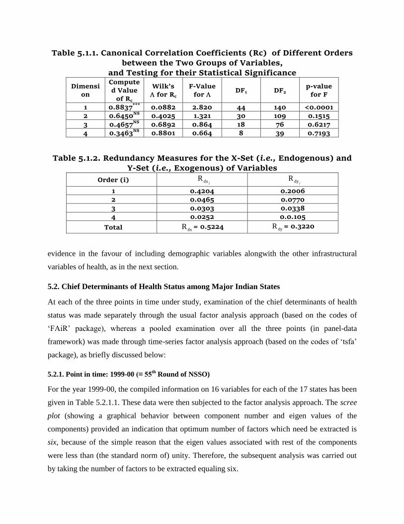
Table 5.1.1. Canonical Correlation Coefficients (Rc) of Different Orders
between the Two Groups of Variables, and Testing for their Statistical Significance
Dimensi
on
Compute
d Value
of Rc
Wilk’s
for Rc
F-Value
for DF1 DF2
p-value
for F
1 0.8837***
0.0882 2.820 44 140 <0.0001
2 0.6450NS
0.4025 1.321 30 109 0.1515
3 0.4657NS
0.6892 0.864 18 76 0.6217
4 0.3463NS
0.8801 0.664 8 39 0.7193
Table 5.1.2. Redundancy Measures for the X-Set (i.e., Endogenous) and Y-Set (i.e., Exogenous) of Variables
Order (i) jdxR
jdyR
1 0.4204 0.2006
2 0.0465 0.0770
3 0.0303 0.0338
4 0.0252 0.0.105
Total dxR = 0.5224 dyR = 0.3220
evidence in the favour of including demographic variables alongwith the other infrastructural
variables of health, as in the next section.
5.2. Chief Determinants of Health Status among Major Indian States
At each of the three points in time under study, examination of the chief determinants of health
status was made separately through the usual factor analysis approach (based on the codes of
‘FAiR’ package), whereas a pooled examination over all the three points (in panel-data
framework) was made through time-series factor analysis approach (based on the codes of ‘tsfa’
package), as briefly discussed below:
5.2.1. Point in time: 1999-00 (≡ 55th
Round of NSSO)
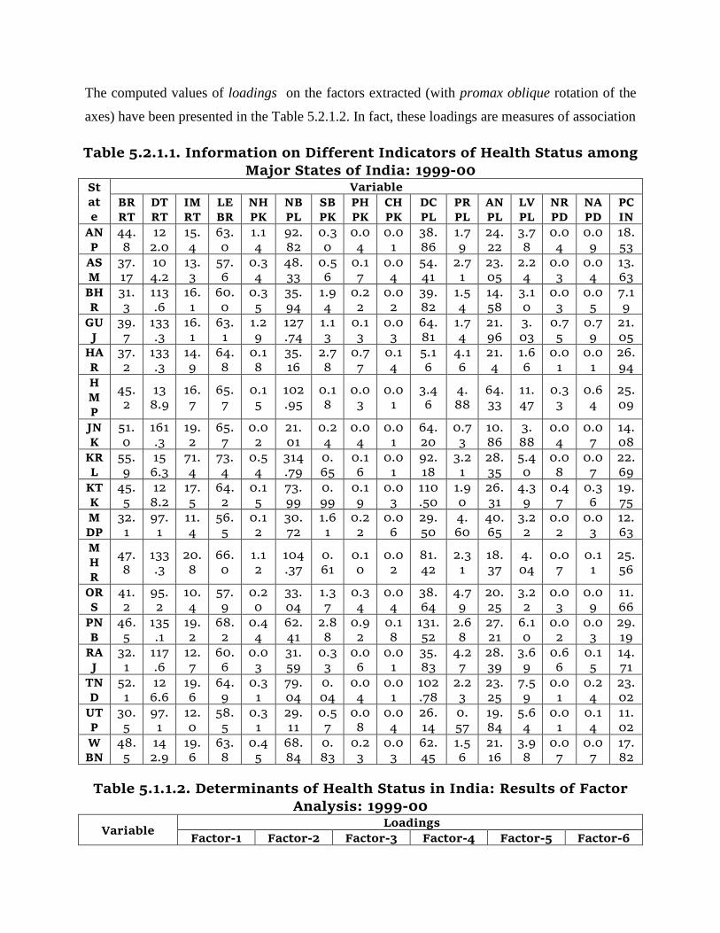
For the year 1999-00, the compiled information on 16 variables for each of the 17 states has been
given in Table 5.2.1.1. These data were then subjected to the factor analysis approach. The scree
plot (showing a graphical behavior between component number and eigen values of the
components) provided an indication that optimum number of factors which need be extracted is
six, because of the simple reason that the eigen values associated with rest of the components
were less than (the standard norm of) unity. Therefore, the subsequent analysis was carried out
by taking the number of factors to be extracted equaling six.
The computed values of loadings on the factors extracted (with promax oblique rotation of the
axes) have been presented in the Table 5.2.1.2. In fact, these loadings are measures of association
Table 5.2.1.1. Information on Different Indicators of Health Status among Major States of India: 1999-00
St
at
e
Variable
BR
RT
DT
RT
IM
RT
LE
BR
NH
PK
NB
PL
SB
PK
PH
PK
CH
PK
DC
PL
PR
PL
AN
PL
LV
PL
NR
PD
NA
PD
PC
IN
AN
P
44.
8
12
2.0
15.
4
63.
0
1.1
4
92.
82
0.3
0
0.0
4
0.0
1
38.
86
1.7
9
24.
22
3.7
8
0.0
4
0.0
9
18.
53
AS
M
37.
17
10
4.2
13.
3
57.
6
0.3
4
48.
33
0.5
6
0.1
7
0.0
4
54.
41
2.7
1
23.
05
2.2
4
0.0
3
0.0
4
13.
63
BH
R
31.
3
113
.6
16.
1
60.
0
0.3
5
35.
94
1.9
4
0.2
2
0.0
2
39.
82
1.5
4
14.
58
3.1
0
0.0
3
0.0
5
7.1
9
GU
J
39.
7
133
.3
16.
1
63.
1
1.2
9
127
.74
1.1
3
0.1
3
0.0
3
64.
81
1.7
4
21.
96
3.
03
0.7
5
0.7
9
21.
05
HA
R
37.
2
133
.3
14.
9
64.
8
0.1
8
35.
16
2.7
8
0.7
7
0.1
4
5.1
6
4.1
6
21.
4
1.6
6
0.0
1
0.0
1
26.
94
H
M
P
45.
2
13
8.9
16.
7
65.
7
0.1
5
102
.95
0.1
8
0.0
3
0.0
1
3.4
6
4.
88
64.
33
11.
47
0.3
3
0.6
4
25.
09
JN
K
51.
0
161
.3
19.
2
65.
7
0.0
2
21.
01
0.2
4
0.0
4
0.0
1
64.
20
0.7
3
10.
86
3.
88
0.0
4
0.0
7
14.
08
KR
L
55.
9
15
6.3
71.
4
73.
4
0.5
4
314
.79
0.
65
0.1
6
0.0
1
92.
18
3.2
1
28.
35
5.4
0
0.0
8
0.0
7
22.
69
KT
K
45.
5
12
8.2
17.
5
64.
2
0.1
5
73.
99
0.
99
0.1
9
0.0
3
110
.50
1.9
0
26.
31
4.3
9
0.4
7
0.3
6
19.
75
M
DP
32.
1
97.
1
11.
4
56.
5
0.1
2
30.
72
1.6
1
0.2
2
0.0
6
29.
50
4.
60
40.
65
3.2
2
0.0
2
0.0
3
12.
63
M
H
R
47.
8
133
.3
20.
8
66.
0
1.1
2
104
.37
0.
61
0.1
0
0.0
2
81.
42
2.3
1
18.
37
4.
04
0.0
7
0.1
1
25.
56
OR
S
41.
2
95.
2
10.
4
57.
9
0.2
0
33.
04
1.3
7
0.3
4
0.0
4
38.
64
4.7
9
20.
25
3.2
2
0.0
3
0.0
9
11.
66
PN
B
46.
5
135
.1
19.
2
68.
2
0.4
4
62.
41
2.8
8
0.9
2
0.1
8
131.
52
2.6
8
27.
21
6.1
0
0.0
2
0.0
3
29.
19
RA
J
32.
1
117
.6
12.
7
60.
6
0.0
3
31.
59
0.3
3
0.0
6
0.0
1
35.
83
4.2
7
28.
39
3.6
9
0.6
6
0.1
5
14.
71
TN
D
52.
1
12
6.6
19.
6
64.
9
0.3
1
79.
04
0.
04
0.0
4
0.0
1
102
.78
2.2
3
23.
25
7.5
9
0.0
1
0.2
4
23.
02
UT
P
30.
5
97.
1
12.
0
58.
5
0.3
1
29.
11
0.5
7
0.0
8
0.0
4
26.
14
0.
57
19.
84
5.6
4
0.0
1
0.1
4
11.
02
W
BN
48.
5
14
2.9
19.
6
63.
8
0.4
5
68.
84
0.
83
0.2
3
0.0
3
62.
45
1.5
6
21.
16
3.9
8
0.0
7
0.0
7
17.
82
Table 5.1.1.2. Determinants of Health Status in India: Results of Factor Analysis: 1999-00
Variable Loadings
Factor-1 Factor-2 Factor-3 Factor-4 Factor-5 Factor-6
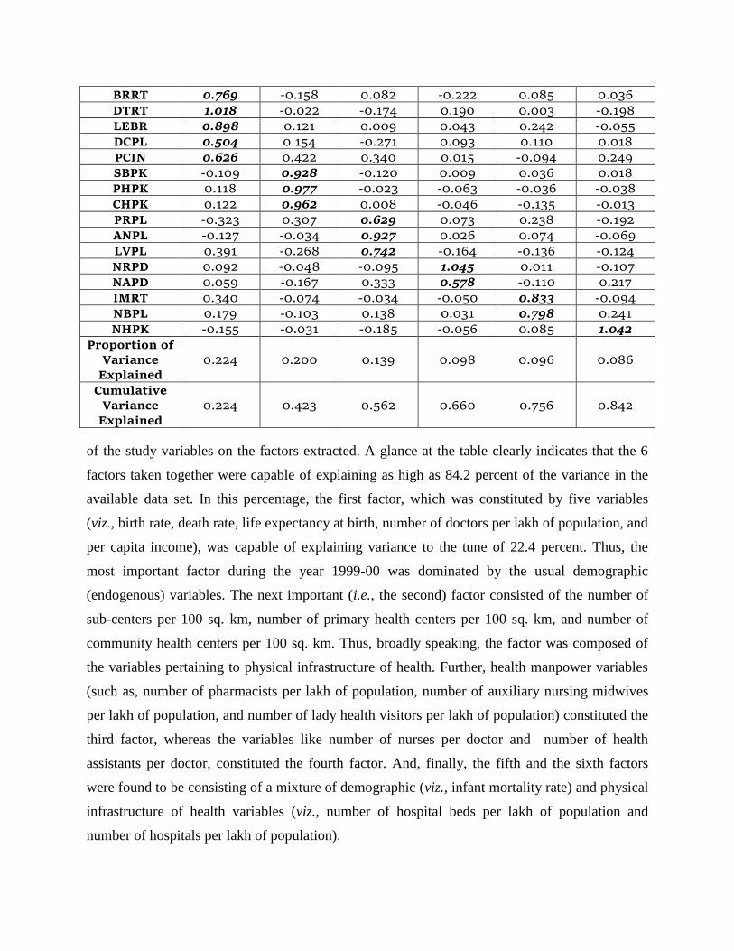
BRRT 0.769 -0.158 0.082 -0.222 0.085 0.036
DTRT 1.018 -0.022 -0.174 0.190 0.003 -0.198
LEBR 0.898 0.121 0.009 0.043 0.242 -0.055
DCPL 0.504 0.154 -0.271 0.093 0.110 0.018
PCIN 0.626 0.422 0.340 0.015 -0.094 0.249
SBPK -0.109 0.928 -0.120 0.009 0.036 0.018
PHPK 0.118 0.977 -0.023 -0.063 -0.036 -0.038
CHPK 0.122 0.962 0.008 -0.046 -0.135 -0.013
PRPL -0.323 0.307 0.629 0.073 0.238 -0.192
ANPL -0.127 -0.034 0.927 0.026 0.074 -0.069
LVPL 0.391 -0.268 0.742 -0.164 -0.136 -0.124
NRPD 0.092 -0.048 -0.095 1.045 0.011 -0.107
NAPD 0.059 -0.167 0.333 0.578 -0.110 0.217
IMRT 0.340 -0.074 -0.034 -0.050 0.833 -0.094
NBPL 0.179 -0.103 0.138 0.031 0.798 0.241
NHPK -0.155 -0.031 -0.185 -0.056 0.085 1.042
Proportion of
Variance
Explained
0.224 0.200 0.139 0.098 0.096 0.086
Cumulative
Variance
Explained
0.224 0.423 0.562 0.660 0.756 0.842
of the study variables on the factors extracted. A glance at the table clearly indicates that the 6
factors taken together were capable of explaining as high as 84.2 percent of the variance in the
available data set. In this percentage, the first factor, which was constituted by five variables
(viz., birth rate, death rate, life expectancy at birth, number of doctors per lakh of population, and
per capita income), was capable of explaining variance to the tune of 22.4 percent. Thus, the
most important factor during the year 1999-00 was dominated by the usual demographic
(endogenous) variables. The next important (i.e., the second) factor consisted of the number of
sub-centers per 100 sq. km, number of primary health centers per 100 sq. km, and number of
community health centers per 100 sq. km. Thus, broadly speaking, the factor was composed of
the variables pertaining to physical infrastructure of health. Further, health manpower variables
(such as, number of pharmacists per lakh of population, number of auxiliary nursing midwives
per lakh of population, and number of lady health visitors per lakh of population) constituted the
third factor, whereas the variables like number of nurses per doctor and number of health
assistants per doctor, constituted the fourth factor. And, finally, the fifth and the sixth factors
were found to be consisting of a mixture of demographic (viz., infant mortality rate) and physical
infrastructure of health variables (viz., number of hospital beds per lakh of population and
number of hospitals per lakh of population).

5.2.2. Point in time: 2004-05 (≡ 61st Round of NSSO)
For the second point in time (i.e., 2004-05, comparable with the time-frame of the 61st Round of
the NSSO), basic data on the study variables are given in Table 5.2.2.1. Here again, the scree
plot indicated the optimum number of factors to be extracted to be six. Results from the
corresponding factor analysis have been given in Table 5.2.2.2. As per the table, the most
significant factor (explaining 22.4 percent, out of the total explained variance of 89.0 percent)
happened to be constituted by six variables, viz., number of hospital beds per lakh of population;
number of auxiliary nursing midwives per lakh of population; number of lady health visitors per
lakh of population; number of nurses per doctor; number of assistants per doctor; and per capita
income. The second factor consisted of number of sub-centers per 100 sq.km; number of primary
health centers per 100 sq. km; and number of community health centers per 100 sq. km. The
factor next in importance was constituted by the demographic variables, viz., birth rate; death
rate; and life expectancy at birth. Thus, during this point in time, the variables pertaining to
health manpower, physical health infrastructure, and demographic traits turned out to be the
significant determinants of health status. Rests of the variables were found to have played
relatively less significant role towards explaining the extent of variance in the data set.
Table 5.2.2.1 Information on Different Indicators of Health Status
among Major States of India: 2004-05 St
at
e
Variable
BR
RT
DT
RT
IM
RT
LE
BR
NH
PK
NB
PL
SB
PK
PH
PK
CH
PK
DC
PL
PR
PL
AN
PL
LV
PL
NR
PD
NA
PD
PC
IN
AN
P
52.
4
13
7.0
17.
5
63.
5
0.1
3
43.
19
0.3
7
0.0
4
0.0
1
43.
58
42.
70
25.
25
4.
25
2.4
3
0.1
0
24.
46
AS
M
40.
0
114
.9
14.
7
58.
1
0.1
3
10.
57
1.0
7
0.1
7
0.0
4
56.
72
8.5
6
21.
28
2.
07
0.6
4
0.0
4
15.
96
BH
R
42.
0
12
3.5
16.
4
60
.7
0.1
1
3.3
4
2.3
9
0.2
1
0.0
4
39.
09
4.5
9
14.
12
3.
01
0.2
5
0.0
8
7.4
1
GU
J
47.
6
14
0.8
18.
5
63.
6
0.2
6
64.
50
1.1
3
0.1
7
0.0
4
70.
62
38.
54
16.
63
2.
88
2.2
4
0.6
3
31.
95
HA
R
47.
6
14
9.3
16.
7
65.
3
0.3
2
31.
40
3.2
1
0.7
3
0.1
5
6.0
5
8.1
9
19.
97
1.9
4
0.4
1
0.0
1
36.
47
H
M
P
75.
2
14
4.9
20.
4
66.
2
0.2
5
119
.72
0.1
8
0.0
6
0.0
2
8.8
9
44.
18
48.
23
9.
86
5.7
2
0.4
5
32.
79
JN
K
69.
9
181
.8
20.
0
66.
2
0.0
3
29.
83
0.1
0
0.0
3
0.0
2
77.
05
10.
15
17.
79
3.5
9
0.7
7
0.0
7
15.
84
KR 67. 15 71. 73. 0.6 87. 0.7 0.2 0.0 115 23. 29. 4. 1.9 0.0 32.

L 6 6.3 4 5 4 50 7 2 5 .76 21 60 97 1 3 08
KT
K
55.
9
14
0.8
20.
0
64.
7
0.4
5
76.
03
0.
87
0.1
5
0.0
2
122
.27
128
.06
21.
11
3.5
8
6.4
4
0.2
4
25.
42
M
DP
45.
5
111
.1
13.
2
57.
1
0.1
1
27.
24
1.8
3
0.1
8
0.0
5
31.
61
2.1
25
25.
45
3.2
8
1.3
5
0.0
4
14.
45
M
H
R
54.
9
14
9.3
27.
8
66.
4
0.2
2
44.
72
0.5
8
0.1
0
0.0
2
93.
44
96.
90
16.
51
4.
45
1.6
8
0.0
9
33.
77
OR
S
61.
3
10
5.3
13.
3
58.
7
0.3
0
34.
89
1.6
9
0.3
1
0.1
1
38.
75
31.
35
26.
20
3.
01
2.2
7
0.0
6
15.
88
PN
B
58.
8
14
9.3
22.
7
68.
6
0.4
9
43.
02
4.
03
0.8
6
0.2
0
135
.41
137
.61
21.
33
5.
69
0.8
7
0.0
3
33.
19
RA
J
42.
0
14
2.9
14.
7
61.
3
0.1
3
34.
90
0.3
3
0.0
5
0.0
1
37.
56
29.
82
23.
81
3.
03
2.3
6
0.1
2
18.
06
TN
D
62.
5
13
5.1
27.
0
65.
4
0.6
9
116
.01
0.
04
0.0
2
0.0
1
110
.34
153
.09
20.
86
6.
29
6.9
5
0.1
8
28.
44
UT
P
37.
7
114
.9
13.
7
59.
2
0.3
8
18.
15
0.
06
0.1
0
0.0
1
26.
60
16.
93
1.4
1
4.1
0
0.2
4
0.1
0
12.
39
W
BN
79.
4
15
6.3
26.
4
64.
1
0.4
6
64.
48
0.
83
0.2
3
0.0
2
63.
28
106
.11
17.
37
2.1
0
0.9
4
0.0
4
22.
22
Table 5.2.2.2. Determinants of Health Status in India: Results of Factor Analysis: 2004-05
Variable Loadings
Factor-1 Factor-2 Factor-3 Factor-4 Factor-5 Factor-6
NBPL 0.671 -0.161 0.041 0.413 -0.044 0.086
ANPL 1.121 0.175 -0.140 -0.388 -0.118 0.188
LVPL 0.764 -0.025 -0.062 0.036 -0.012 0.046
NRPD 0.718 -0.222 -0.222 0.165 0.257 -0.166
NAPD 0.630 -0.145 0.029 -0.176 0.023 -0.278
PCIN 0.438 0.371 0.354 0.133 -0.019 0.031
SBPK 0.005 0.973 -0.136 -0.104 0.115 -0.077
PHPK -0.135 0.983 0.079 0.211 -0.063 -0.115
CHPK 0.035 0.998 -0.075 0.041 0.032 -0.037
BRRT 0.291 -0.069 0.512 0.123 -0.077 0.049
DTRT -0.244 -0.111 1.241 -0.288 0.022 -0.090
LEBR 0.106 0.078 0.618 0.068 0.121 0.368
NHPK -0.057 0.117 -0.245 1.077 0.010 0.288
DCPL -0.052 0.009 0.044 -0.165 1.043 0.290
PRPL 0.062 0.112 0.091 0.290 0.609 -0.283
IMRT 0.091 -0.183 -0.001 0.290 0.079 0.920
Proportion of
Variance
Explained
0.224 0.204 0.155 0.120 0.099 0.088
Cumulative
Variance
Explained
0.224 0.428 0.583 0.703 0.802 0.890
5.2.3. Point in time: 2011-12 (≡ 68th
Round of NSSO)

The basic information on different indicators of health status for the third point in time (i.e.,
2011-12, which had a close comparability with the 68th
Round of NSSO) is presented in Table
5.2.3.1. Results from factor analysis as applied to these data have been given in Table 5.2.3.2.
Table 5.2.3.1 Information on Different Indicators of Health Status among Major States of India: 2011-12
St
at
e
Variable
BR
RT
DT
RT
IM
RT
LE
BR
NH
PK
NB
PL
SB
PK
PH
PK
CH
PK
DC
PL
PR
PL
AN
PL
LV
PL
NR
PD
NA
PD
PC
IN
AN
P
54.
6
13
3.3
20.
4
64.
2
0.1
7
45.
42
4.5
5
0.5
7
0.
06
74.
42
52.
47
33.
74
4.1
6
2.1
9
0.0
6
29.
57
AS
M
42.
4
116
.3
16.
4
59.
0
0.2
0
24.
84
5.8
5
1.0
8
0.1
4
62.
30
7.9
2
30.
09
1.9
4
0.7
7
0.0
3
18.
77
B
H
R
35.
1
13
7.0
19.
2
61.
3
1.8
2
22.
16
9.
41
1.8
9
0.
07
36.
68
4.1
0
10.
05
1.1
0
0.2
5
0.0
3
11.
02
G
UJ
44.
8
14
5.0
20.
8
64.
1
0.1
9
48.
81
3.7
1
0.5
5
0.1
4
78.
27
35.
31
19.
07
2.7
5
1.9
0
0.5
8
40.
91
H
AR
44.
1
14
4.9
19.
6
66.
1
0.3
5
31.
20
16.
45
0.9
9
0.2
1
16.
36
28.
71
25.
98
2.2
4
0.3
8
0.0
1
48.
64
H
M
P
58.
1
13
5.1
22.
2
66.
9
0.2
6
117.
52
3.7
2
0.8
1
0.1
3
18.
22
41.
60
43.
84
2.2
3
2.0
7
0.0
4
42.
37
JN
K
53.
8
17
2.4
22.
2
66.
9
0.0
4
32.
11
0.
86
0.1
7
0.
04
91.
50
17.
64
19.
68
1.1
4
7.2
9
0.1
7
17.
7
KR
L
68.
0
151
.5
83.
3
73.
9
0.9
9
94.
15
11.
77
1.7
9
0.5
9
144
.82
53.
07
24.
00
3.7
3
1.7
8
0.4
0
43.
71
KT
K
51.
3
13
5.1
24.
4
65.
4
0.4
8
105
.80
4.2
5
1.1
4
0.1
7
144
.94
131
.97
19.
57
2.
60
1.5
6
0.1
4
32.
72
M
DP
36.
1
116
.3
14.
9
58.
0
0.1
5
40.
04
2.
88
0.3
7
0.1
1
37.
31
1.9
3
23.
61
0.
67
1.1
1
0.0
1
14.
65
M
H
R
56.
8
151
.5
32.
3
67.
2
0.5
8
45.
16
3.4
4
0.5
9
0.1
2
124
.48
95.
94
26.
04
6.1
4
1.6
5
0.1
2
39.
37
OR
S
47.
6
111
.1
15.
4
59.
6
1.2
6
38.
36
4.
94
0.9
4
0.1
7
40.
54
34.
57
20.
44
2.2
4
2.4
6
0.0
4
22.
08
PN
B
58.
8
13
8.9
26.
3
69.
4
0.4
6
38.
83
5.8
6
0.7
8
0.2
6
140
.53
129
.03
25.
361
2.
98
0.7
7
0.0
1
41.
03
RA
J
36.
8
14
7.1
16.
9
61.
9
0.1
4
47.
65
3.2
0
0.4
4
0.1
1
42.
37
27.
06
27.
52
3.
08
2.2
4
0.1
2
22.
45
TN
D
61.
3
13
5.1
35.
7
66.
2
0.4
5
66.
38
6.
69
0.9
8
0.2
0
122
.11
213
.74
18.
05
2.5
6
6.5
6
0.0
6
34.
6
UT
P
34.
8
119
.1
15.
9
59.
9
0.3
6
28.
77
8.5
2
1.5
3
0.2
1
29.
57
15.
45
1.1
4
0.
21
0.2
4
0.0
9
14.
74
W
BN
58.
1
161
.3
30.
3
65.
0
0.3
3
60.
73
11.
67
1.0
4
0.3
8
65.
29
99.
41
19.
14
1.2
4
0.8
4
0.0
2
27.
99

Table 5.2.3.2. Determinants of Health Status in India: Results of Factor
Analysis: 2011-12
Variable Loadings
Factor-1 Factor-2 Factor-3 Factor-4 Factor-5 Factor-6
BRRT 0.563 0.181 0.444 -0.233 0.130 -0.017
NBPL 0.595 0.076 0.157 0.048 -0.186 -0.035
ANPL 1.275 -0.233 -0.430 -0.327 -0.083 0.006
LVPL 0.569 -0.154 0.178 0.198 -0.092 0.076
LEBR 0.413 0.225 0.221 0.092 0.389 0.205
IMRT 0.331 0.727 -0.112 0.173 0.089 -0.133
NHPK -0.263 0.545 0.025 -0.039 -0.167 -0.061
SBPK -0.009 0.839 -0.070 -0.243 0.233 0.707
PHPK -0.256 0.876 0.024 -0.046 -0.214 0.144
CHPK 0.183 0.841 -0.005 0.068 -0.003 0.178
DCPL -0.085 0.021 0.742 0.160 -0.040 -0.215
PRPL -0.090 -0.082 1.252 -0.298 -0.123 0.166
NRPD -0.114 -0.337 0.328 -0.092 0.299 -0.424
NAPD -0.197 -0.060 -0.286 1.143 0.044 0.009
DTRT -0.072 -0.081 -0.139 0.044 1.118 0.089
PCIN 0.645 -0.016 0.311 0.283 -0.022 0.695
Proportion of
Variance
Explained
0.222 0.206 0.183 0.114 0.107 0.085
Cumulative
Variance
Explained
0.222 0.429 0.612 0.726 0.833 0.918
Scree plot for the analysis has, once again, provided an indication towards the acceptance of six
factors for extraction. As per the results (Table 5.1.3.2), nearly one-fourth (22.2 percent) of the
total explained variance (of 91.8 percent) was attributable to the most significant (i.e., the first)
factor, which happened to be a mixture of usual demographic indicators (like, birth rate and life
expectancy at birth), physical health infrastructure (like, number of hospital beds per lakh of
population), and health manpower statistics (such as, number of auxiliary nursing midwives per
lakh of population and number of lady health visitors per lakh of population). Notably, the next
most-significant factor (associated with variance explanation of nearly 21 percent) was broadly
made up of physical health infrastructure variables (such as, number of hospitals per 100 sq.km,
number of sub-centers per lakh of population, number of primary health centers per lakh of
population, and number of community health centers per lakh of population). The remaining four
factors were far from being explicit in nature, as these involved a mixture of the types of
dimensions.
5.2.4. Pooled Analysis

Next, in order to squeeze out the overall picture on major determinants of health, the information
at all the three points in time (in panel data frame work) was subjected to time series factor
analysis. The analysis was capable of extracting a totality of five factors, which together could
explain 67.4 percent of the variance in the data set (Table 5.2.4.1).
Table 5.2.4.1. Determinants of Health Status in India: Pooled Results of Time Series Factor Analysis
Variable Loadings
Factor-1 Factor-2 Factor-3 Factor-4 Factor-5
SBPK 0.971 -0.104 0.001 0.044 0.060
PHPK 0.873 0.067 0.009 -0.076 -0.061
CHPK 0.841 0.143 0.073 0.056 -0.045
IMRT 0.120 0.830 -0.130 -0.050 0.066
LEBR 0.052 0.795 -0.099 0.054 0.364
NBPL -0.192 0.638 -0.096 0.234 -0.081
DCPL -0.126 0.640 0.413 -0.296 -0.084
PRPL 0.086 -0.045 1.071 -0.062 -0.151
NRPD -0.121 -0.183 0.658 0.070 0.094
ANPL 0.144 -0.153 -0.061 0.983 -0.130
LVPL -0.328 0.263 0.025 0.587 -0.154
DTRT -0.016 0.241 -0.132 -0.209 1.001
BRRT -0.073 0.276 0.358 0.072 0.315
NHPK 0.174 0.414 -0.053 -0.193 -0.193
NAPD -0.093 0.017 -0.097 0.320 0.097
PCIN 0.462 0.262 0.251 0.379 0.092
Prop. of
Variance
Explained
0.181 0.167 0.126 0.113 0.087
Cum. Prop.
of Variance
Explained
0.181 0.348 0.474 0.587 0.674
As regards constitution of the factors, the first factor (which could explain 18.1 percent of the
variance) was constituted by three variables viz., number of sub-centers per 100 sq km; number
of primary health centers per 100 sq km; and number of community health centers per 100 sq
km. Clearly, each of the constituent variables of the most important factor referred to the
physical infrastructure of health. The next important factor (having accounted for 16.7 percent of
the variance explained) was composed of four variables, viz., infant mortality rate; life
expectancy at birth; number of hospital beds per lakh of population; and number of doctors per
lakh of population. The factor, obviously, happened to be a synthesis of physical & social health
infrastructure, as also demographic variables. The third factor (capable of explaining 12.6

percent of the variance) was made up of two variables of social infrastructure: number of
pharmacists per lakh of population; and number of nurses per doctor. Similarly, the fourth factor
(responsible for explaining 11.3 percent of the variance), too, consisted of another couple of
variables of social infrastructure, viz., number of auxiliary nursing midwives per lakh of
population; and number of lady health visitors per lakh of population. And, the last significant
factor (accounting for 8.7 percent of the variance explained) consisted of the lone demographic
variable – death rate. Notably, as per the results of the pooled analysis, rest of the four variables
(viz., birth rate; number of hospitals per 100 sq km; number of assistants per doctor; and per
capita income), in the presence of the rest of the 12 variables, failed to show their importance
while determining the health status of a state.
The analysis has thus provided us with an evidence that relative significance of different
parameters of health status among the Indian states has not remained time invariant, but has
instead undergone a drastic reshuffling during the study span. As per the pooled analysis, the
most important dimension of health among the major Indian states is composed of the parameters
of physical health infrastructure, followed by those of social health infrastructure.
5.3. Relative Positioning of the Major Indian States – Construction of the Composite Index
In order to examine the relative positioning of the major Indian states, as also to study temporal
shifts, if any, in the positioning at each of the points in time (as also over the entire study period
taken together), the composite index of health status was constructed through the methodology as
outlined in Section 4.2 above (Table 5.3.1). A glance at the table shows that in the year 1999-00,
Punjab (with a value of 4.57 for the index) occupied the top position, followed next by Kerala
Table 5.3.1. Composite Index of Health Status among the Major Indian States
State
1999-00 2004-05 2011-12 Pooled
Composite
Index Rank
Composite
Index Rank
Composite
Index Rank
Composite
Index Rank
ANP 3.246 11 2.334 12 2.666 9 2.659 9
ASM 2.942 16 1.978 16 2.315 15 2.064 14
BHR 2.958 15 2.027 15 2.340 14 1.914 15
GUJ 3.714 5 2.659 7 2.630 10 2.827 8
HAR 3.937 3 2.859 6 2.739 8 2.125 12
HMP 3.885 4 3.366 2 2.933 7 2.996 7
JNK 3.340 10 2.339 11 2.368 12 2.612 10
KRL 4.274 2 3.230 3 4.076 1 4.436 1
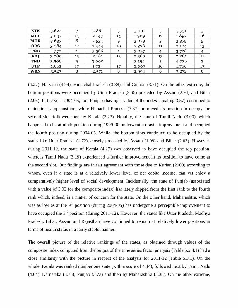
KTK 3.622 7 2.861 5 3.001 5 3.751 3
MDP 3.042 14 2.147 14 1.909 17 1.892 16
MHR 3.637 6 2.534 9 3.029 3 3.379 5
ORS 3.084 12 2.444 10 2.378 11 2.104 13
PNB 4.572 1 3.566 1 3.027 4 3.728 4
RAJ 3.080 13 2.181 13 2.360 13 2.265 11
TND 3.508 9 3.000 4 3.194 2 4.036 2
UTP 2.662 17 1.724 17 2.007 16 1.766 17
WBN 3.527 8 2.571 8 2.994 6 3.232 6
(4.27), Haryana (3.94), Himachal Pradesh (3.88), and Gujarat (3.71). On the other extreme, the
bottom positions were occupied by Uttar Pradesh (2.66) preceded by Assam (2.94) and Bihar
(2.96). In the year 2004-05, too, Punjab (having a value of the index equaling 3.57) continued to
maintain its top position, while Himachal Pradesh (3.37) improved its position to occupy the
second slot, followed then by Kerala (3.23). Notably, the state of Tamil Nadu (3.00), which
happened to be at ninth position during 1999-00 underwent a drastic improvement and occupied
the fourth position during 2004-05. While, the bottom slots continued to be occupied by the
states like Uttar Pradesh (1.72), closely preceded by Assam (1.99) and Bihar (2.03). However,
during 2011-12, the state of Kerala (4.27) was observed to have occupied the top position,
whereas Tamil Nadu (3.19) experienced a further improvement in its position to have come at
the second slot. Our findings are in fair agreement with those due to Kurian (2000) according to
whom, even if a state is at a relatively lower level of per capita income, can yet enjoy a
comparatively higher level of social development. Incidentally, the state of Punjab (associated
with a value of 3.03 for the composite index) has lately slipped from the first rank to the fourth
rank which, indeed, is a matter of concern for the state. On the other hand, Maharashtra, which
was as low as at the 9th
position (during 2004-05) has undergone a perceptible improvement to
have occupied the 3rd
position (during 2011-12). However, the states like Uttar Pradesh, Madhya
Pradesh, Bihar, Assam and Rajasthan have continued to remain at relatively lower positions in
terms of health status in a fairly stable manner.
The overall picture of the relative rankings of the states, as obtained through values of the
composite index computed from the output of the time series factor analysis (Table 5.2.4.1) had a
close similarity with the picture in respect of the analysis for 2011-12 (Table 5.3.1). On the
whole, Kerala was ranked number one state (with a score of 4.44), followed next by Tamil Nadu
(4.04), Karnataka (3.75), Punjab (3.73) and then by Maharashtra (3.38). On the other extreme,

the states like Uttar Pradesh (1.77), Madhya Pradesh (1.89), Bihar (1.91), Assam (2.06) and
Odisha (2.10) have occupied the bottom positions on health traits.
5.4. Calorie Inequalities among the Major Indian States
For measuring calorie inequalities among the states, we have made use of the data on the
distribution of households by calorie intake level for different MPCE (separately for rural and
urban regions) of each of the states under study. For the purpose of clarification on the format of
data used, we have presented such a distribution for rural regions of India as whole in respect of
55th
Round of NSSO (Table 5.4.1).
Table 5.4.1. Per Thousand Distribution of Households by Calorie Intake Level for Each MPCE Class in Rural India – 55th Round
MPCE
Class
(Rs)
Calorie Intake Level
70 70-
80
80-
90
90-
100
100-
110
110-
120
120-
150 150
All
Classes
SMP
HHS
225 654 177 98 44 13 7 3 3 1000 2547
225-
255 416 239 185 93 40 16 9 3 1000 2451
255-
300 311 231 200 134 66 28 23 7 1000 5147
300-
340 182 207 231 173 104 48 43 11 1000 5588
340-
380 145 181 225 179 127 69 61 14 1000 5892
380-
420 96 153 190 199 149 94 96 23 1000 5895
420-
470 71 115 170 200 161 110 131 42 1000 6783
470-
525 53 90 150 176 171 127 173 60 1000 6635
525-
615 37 72 130 156 161 134 222 88 1000 8253
615-
775 27 46 88 134 145 141 274 145 1000 9383
775-
950 19 34 61 110 126 126 295 230 1000 5337
950 23 16 44 69 107 107 271 381 1000 7474
All
classes 134 124 151 149 92 92 143 82 1000 69206
The computed values of calorie inequalities, as estimated through the FGT(2) measure (equation
10) have been exhaustively presented in Table 5.4.2. As per the table, there obviously have
been wide inequalities in the calorie intake at different levels: between states, between rounds

Table 5.4.2. Computed Values of FGT(2) Index of Inequality among
Major Indian States during the Three Rounds – Rural, Urban and Combined Regions
State
Rural Urban Combined
Round Mean
Round Mean
Round Mea
n 55th
61st
68st
55th
61st
68st
55th
61st
68st
ANP 0.03
26
0.032
8
0.01
58
0.027
1
0.03
69
0.046
8
0.008
9
0.030
9
0.03
48
0.03
98
0.01
24
0.02
90
ASM 0.04
61
0.025
3
0.02
52
0.032
2
0.02
98
0.028
4
0.010
5
0.022
9
0.03
80
0.02
68
0.01
78
0.02
76
BHR 0.02
83
0.024
9
0.02
20
0.025
1
0.02
63
0.030
4
0.010
3
0.022
3
0.02
73
0.02
76
0.01
61
0.02
37
GUJ 0.03
37
0.039
9
0.02
73
0.033
6
0.03
28
0.041
6
0.011
0
0.028
5
0.03
32
0.04
07
0.01
92
0.03
10
HAR 0.01
58
0.022
2
0.01
06
0.016
2
0.02
95
0.040
7
0.007
5
0.025
9
0.02
26
0.03
14
0.00
90
0.02
10
HMP 0.00
85
0.009
5
0.00
18
0.006
6
0.00
92
0.015
4
0.002
8
0.009
1
0.00
88
0.01
24
0.00
23
0.00
79
JNK 0.00
88
0.010
2
0.00
73
0.008
8
0.00
82
0.009
1
0.003
5
0.006
9
0.00
85
0.00
96
0.00
54
0.00
79
KRL 0.03
99
0.039
1
0.02
22
0.033
7
0.03
93
0.051
6
0.012
6
0.034
5
0.03
96
0.04
54
0.01
74
0.03
41
KTK 0.04
18
0.046
1
0.01
70
0.035
0
0.03
94
0.046
6
0.011
1
0.032
4
0.04
06
0.04
64
0.01
40
0.03
37
MDP 0.03
51
0.038
9
0.02
09
0.031
6
0.03
38
0.040
0
0.011
2
0.028
3
0.03
44
0.03
94
0.01
60
0.03
00
MHR 0.03
37
0.041
6
0.01
39
0.029
7
0.03
44
0.050
6
0.009
4
0.031
5
0.03
40
0.04
61
0.01
16
0.03
06
ORS 0.02
32
0.035
7
0.01
39
0.024
3
0.01
68
0.037
0
0.008
1
0.020
6
0.02
00
0.03
64
0.01
10
0.02
24
PNB 0.01
57
0.018
4
0.00
75
0.013
9
0.02
52
0.031
0
0.008
4
0.021
5
0.02
04
0.02
47
0.00
79
0.01
77
RAJ 0.01
20
0.018
7
0.01
01
0.013
6
0.02
05
0.028
5
0.007
9
0.019
0
0.01
62
0.02
36
0.00
90
0.01
63
TND 0.05
50
0.045
6
0.02
59
0.042
2
0.04
72
0.050
4
0.012
4
0.036
7
0.05
11
0.04
80
0.01
92
0.03
94
UTP 0.01
97
0.015
9
0.00
25
0.012
7
0.03
26
0.035
6
0.012
9
0.027
0
0.02
62
0.02
58
0.00
77
0.01
99
WBN 0.02
84
0.022
2
0.01
79
0.022
8
0.03
13
0.039
5
0.011
3
0.027
4
0.02
98
0.03
08
0.01
46
0.02
51
Mean 0.02
81
0.028
6
0.01
54
0.024
1
0.02
90
0.036
7
0.009
4
0.025
0
0.02
86
0.03
26
0.01
24
0.02
45
between regions. For instance, within rural regions, the extent of inequalities during 55th
round
was as low as 0.0085 in Himachal Pradesh, but was as high as 0.0550 in Tamil Nadu. Further,
within urban regions, the extent of inequalities in Maharashtra was as high as 0.0506 during 61st
round, but was a mere 0.0094 during 68th
round. Similarly, within Uttar Pradesh state, the extent
of inequalities during 68th
round was a mere 0.0025 among rural regions, but was comparatively
much higher at 0.0129 among urban regions.
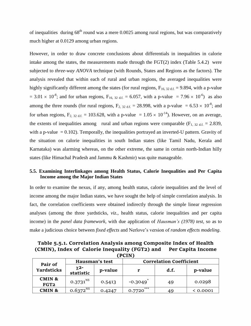
However, in order to draw concrete conclusions about differentials in inequalities in calorie
intake among the states, the measurements made through the FGT(2) index (Table 5.4.2) were
subjected to three-way ANOVA technique (with Rounds, States and Regions as the factors). The
analysis revealed that within each of rural and urban regions, the averaged inequalities were
highly significantly different among the states (for rural regions, F16, 32 d.f. = 9.894, with a p-value
= 3.01 10-8
; and for urban regions, F16, 32 d.f. = 6.057, with a p-value = 7.96 10-6
) as also
among the three rounds (for rural regions, F2, 32 d.f. = 28.998, with a p-value = 6.53 10-8
; and
for urban regions, F2, 32 d.f. = 103.628, with a p-value = 1.05 10-14
). However, on an average,
the extents of inequalities among rural and urban regions were comparable (F1, 32 d.f. = 2.839,
with a p-value = 0.102). Temporally, the inequalities portrayed an inverted-U pattern. Gravity of
the situation on calorie inequalities in south Indian states (like Tamil Nadu, Kerala and
Karnataka) was alarming whereas, on the other extreme, the same in certain north-Indian hilly
states (like Himachal Pradesh and Jammu & Kashmir) was quite manageable.
5.5. Examining Interlinkages among Health Status, Calorie Inequalities and Per Capita
Income among the Major Indian States
In order to examine the nexus, if any, among health status, calorie inequalities and the level of
income among the major Indian states, we have sought the help of simple correlation analysis. In
fact, the correlation coefficients were obtained indirectly through the simple linear regression
analyses (among the three yardsticks, viz., health status, calorie inequalities and per capita
income) in the panel data framework, with due application of Hausman’s (1978) test, so as to
make a judicious choice between fixed effects and Nerlove’s version of random effects modeling.
Table 5.5.1. Correlation Analysis among Composite Index of Health
(CMIN), Index of Calorie Inequality (FGT2) and Per Capita Income (PCIN)
Pair of Yardsticks
Hausman’s test Correlation Coefficient
2-statistic
p-value r d.f. p-value
CMIN & FGT2
0.3731NS 0.5413 -0.3049* 49 0.0298
CMIN & 0.6372NS 0.4247 0.7720*** 49 < 0.0001

PCIN
FGT2 & PCIN
0.6293NS 0.4276 -0.2512NS 49 0.0754
NS:
Non-significant; *: Significant at 5% probability level; ***: Significant at 0.1%
probability level;
In each of the three pairs, non-significance of the 2-statistic for Hausman’s test (Table 5.5.1)
suggested that the more versatile random effects modeling be preferred. As per the modeling,
association between the composite index of health status (CMIN) and FGT(2) measure of the
inequalities was observed to be indirect (r = -0.3049) and statistically significant ( p = 0.0298).
Further, there was a feeble indication of an indirect association between the measure of
inequalities and per capita income (r = -0.2512; p = 0.0754). However, the association between
the composite index of health and per capita income was direct (r = 0.7720) and very robust (p-
value < 0.0001). Thus the states with better health status have shown a very strong tendency to
be associated with higher income level and, that; such states would expectedly have less severe
incidence of calorie inequalities.
6. Conclusion and Policy Implications
As per the results, the chief determinants of health status have undergone voluminous reshuffling
during the study span, from usual demographic indicators to those of physical and social health
infrastructure. Within each of rural and urban regions, the averaged inequalities were seen to be
highly significantly different among the states as also among the three rounds of NSSO.
However, on an average, the extents of inequalities among rural and urban regions were
comparable. Further, the states with better health status showed a very strong tendency to be
relatively richer and low in the extent of calorie inequalities. Thus, as a policy measure, there is a
dire need for shifting priorities in favour of investment on both physical and social health
infrastructure, particularly in laggard states and in those states which have undergone a rapid
slippage in their ranking. If the state alone cannot shoulder the burden of increased expenditure
on this important economic activity, then public-private-partnership model needs be propagated.
Improved health conditions would expectedly enhance incomes of the people which, in turn,
might bring down the severity of inequalities in calorie intake.
References
Akbas, Y. and C. Takma (2005). “Canonical Correlation Analysis for Studying the Relationship
between Egg Production Traits and Body Weight, Egg Weight and Age at Sexual
Maturity in Layers”, Czech J. Anim. Sci, Vol. 50, No.4: 163-8.
Au, David H., M. B. McDonnell, D. C. Martin, and S. D. Fihn. 2001. “Regional Variations in
Health Status.” Medical Care 39(8): 879–88.
Bardhan P K (1974a), “The Pattern of Income distribution in India: A Review”, in T N
Srinivasan and P K Bardhan (Eds.), Poverty and Income Distribution in India, Statistical
Publishing Society, Calcutta: 103-38.
—————— (1974b), “On the Incidence of Poverty in Rural India in the Sixties”, in T N
Srinivasan and P K Bardhan (Eds.), Poverty and Income Distribution in India, Statistical
Publishing Society, Calcutta: 264-80.
Chadha, G.K. (2007), “Changing Structure of Demand for Agricultural Commodities: Preparing
for the Future”, Indian Journal of Agriultural Market, Vol. 21(1):1-42.
Chatterjee, G S, and N Bhattacharya (1974), “On Disparities in Per Capita Household
Consumption in India” in T R Srinivasan and P K Bardhan (Eds.), Poverty and Income
Distribution in India, Statistical Publishing Society, Calcutta: 337-68.
Dandekar, V M and N Rath (1971), “Poverty in India”, Indian School of Political Economy.
Pune. (First published in Economic and Political Weekly, Vol. 6 (1 & 2).
Das, A. (1999). “Socio-Economic Development in India: A Regional Analysis”, Development
and Society, Vol. 28(2):313-45.
Dasgupta, R (1983), “Estimation of Nutritional Intakes”. Economic and Political Weekly, Vol.
18 (28): 1238-45.
————— (1984), “Nutritional Situation in India — A Statistical Analysis”, Economic and
Political Weekly, Vol. 19 (34): 1491-4.
Datta, T. N., & B. K. Ganguly. (2002). “An analysis of consumer expenditure pattern in Indian
states with special reference to milk and milk products.” Indian Dairyman, 54(9), 47–56.
Foster J, J Greer, and E Thorbecke (1984), “Notes and Comments : A Class of Decomposable
Poverty Measures” Econometrica, Vol. 52(3): 761-6.
Foster J, J Greer, and E Thorbecke (2010), “The Foster-Greer-Thorbecke Poverty Measures:
Twenty Five Years Later” Institute for International Economic Policy Working Paper
Series, The George Washington University.
Ghassemi, H. (1972). “Food Intake Study of Pre-school Children”, University of Tehran, School
of Public Health, Tehran.
Gilbert, P. and E. Meijer (2012), “Package ‘tsfa’, contributed to R-Project (http://tsanalysis.r-
forge.r-project.org/)
Giri, A K (2006), “Cereal Consumption Over Time in the Country and Across the States”, Indian
Journal of Agricultural Economics, Vol. 61(3): 389-98.
Goodrich, B. (2012), “The Package ‘FAiR”, contributed to R-Project (http://wiki.r-
project.org/rwiki/doku.php?id=packages:cran:fair)
Gorusch, R.L. (1974), Factor Analysis (Philadelphia: Saunders, Ken & Georgie).
Gopalon, C (1970), “Some Recent Studies in the Nutrition Research Laboratories, Hyderabad”,
American Journal of Clinical Nutrition, Vol. 23(1): 35-51.
Gopalan C, B V Ramasastri and S C Balasubramanian (1971), “Nutritive Value of Indian Foods
— Health and Fitness”, National Institute of Nutrition (Indian Council of Medical
Research), Hyderabad.
Gupta, D. (2009), “Disparities in Development, Status of Women and Social Opportunities:
Indian Experience”, Journal of Alternative Perspectives in the Social Sciences, Vol. 1(3):
687-719.
Hausman, E. (1978). “ Specification Tests in Econometrics”, Econometrica, 46(1): 1251-71.
Hotelling, H. (1935). “The Most Predictable Criterion,” Journal of Education
Psychology,Vol.26: 139-42.
Kathuria, V. and D. Sankar (2005), “Inter-State Disparities in Health Outcomes in Rural India:
An Analysis Using a Stochastic Production Frontier Approach”, Development Policy
Review, Vol. 23 (2): 145-63.
Kumar, P., Mruthyunjaya, & M. M. Dey. (2007). “Long-term changes in Indian food basket and
nutrition.” Economic and Political Weekly, 42(35), 3567–3572.
Kumar, N. P. (2011). “Status of Women and Economic Development: A decadal Analysis Based
on Indian States”, Socio-economic Voices: 1-23.
Kumari, R. (2011). “Inter-District Disparity in Health Care Facility and Education: A Care of
Uttar Pradesh”, Journal of Education and Practice, Vol. 2(1): 38-56.
Kurian, N. J. (2000), “Widening Regional Disparities in India − Some Indicators”, Economic and
Political Weekly, 35(7) (Feb. 12-18): 538-50.
Lindeman, R.H., P.F. Merenda and R.Z. Gold (1980). Introduction to Bivariate and Multivariate
Analysis (London, Foresman and Co.).
Mendes, M., A. Karabayir, I.E. Erbil and T. Savas ( 2005), “The relationship among pre-and post
slaughter traits of American Bronze Turkey. Archiv fur Tierzucht-Archives of Animal
Breeding , Vol. 48: 283-9.
Mittal, S (2007), “What Affect Changes in Cereal Consumption?” Economic and Political
Weekly, Vol. 42(5): 444-7.
Musebe, O. R., & P. Kumar. (2006). “Food expenditure pattern of rural household in Andhra
Pradesh.” Indian Journal of Agricultural Marketing, 20(1), 131–139.
Nair, K.R.G (2007). “Malnourishment among Children in India: Regional Analysis.” Economic
and Political Weekly, Vol. XLII (37): 3797-804.
Nasurudeen, P, A Kuruvilla, R Sendhil, and V Chandrasekar (2006), “The Dynamics and
Inequality of Nutrient Consumption in India” Indian Journal of Agricultural Economics
Vol. 61(3): 362-73.
Nerlove, M. (1971). “Further Evidence on the Estimation of Dynamic Economic Relations from
a Time-Series of Cross-Sections”, Econometrica, Vol. 39: 359–82.
OECD (2008), Handbook on Constructing Composite Indicators: Methodology and User Guide
(Ispra, Italy: Joint Research Centre of the European Commission).
Osberg, L and Kuan, Xu (2008), “How Should We Measure Poverty in a Changing World?
Methodological Issues and Chinese Case Study” Review of Development Economics, Vol.
12(2): 419-41.

Pathak, P. and K. K. Gaur (1997). “A Composite Index-based Approach for Analysis of the
Health System in the Indian Context”, Indian Institute of Health Management Research,
Working Paper No. 2: 1-26.
Randhawa, G. S., & S. S. Chahal. (2005). “Consumption pattern of milk and milk products in
rural Punjab.” Indian Journal of Agricultural Economics, 61(3), 141–149.
Rao S.K. (1971). “Inter-regional Variations in Agricultural Growth, 1952-53 to 1964-65: A
Tentative Analysis in Relation to Irrigation”, Economic and Political Weekly, Vol. 6:
1333-46. Rao, S.K. (1973). “A Note on Measuring Economic Distances Betweeen Regions in India”,
Economic and Political Weekly, April 1973.
Rao, V. K. R. V. 1981. “Some Nutritional Puzzles: A Note.” Economic and Political Weekly
16(28/29): 1205+1207–8.
Rao, C. H. (2000). “Declining demand for food grains in rural India: Causes and implications.”
Economic and Political Weekly, 35(4), 201–206.
Ravallion, M (1992), “Does Undernutrition Respond to Income and Prices? Dominance Tests for
Indonesia”, The World Bank Economic Review, Vol. 6 (1): 109-24.
Raykov, T. and G. A. Marcoulides (2008). An Introduction to Applied Multivariate Analysis
(New York: Routledge Taylor & Francis Group).
Roy, T K, S Kumar and Y Vaidehi (2004), “Social Inequalities in Health and Nutrition in
Selected States”, Economic and Political Weekly, Vol. 34 (7): 677-83.
Sarkar, P.C. (1994). “Regional Imbalances in Indian Economy”, Economic and Political Weekly,
Vol. 29(11): 621-33.
Sethi, A.S. (2003a), “Determinants of Poverty at the Global Level (With Special Reference to
India)”, in the 86th Annual Conference Volume of the Indian Economic Association :
480-91.
Sethi, A.S. and Sanjeev Kumar (2013), “Co-operative Banking and Rural Development in
Punjab – An Examination of Interdependencies through Canonical Correlation
Approach”, The Journal of Income and Wealth , 35 (2): 10-21.
Sethi, A.S. and R. Pandhi (2011a), “Differential Inequalities in Calorie Intake among Indian
States: Evidence From Different Rounds of NSS”, Proceedings of the Annual
Conference of the Indian Association for Research in National Income and Wealth at the
Centre for Economic and Social Studies, Hyderabad (March 11-13): Article No B1.
Sethi, A.S. and R. Pandhi (2011b), “Nutritional Expenditure among Indian States: An
Evidence from Divergence Analysis”, Indian Economic Journal (Special Issue on
Enhancing Human Resources for Inclusive Growth, Employment and Welfare, released
during the 94th
Annual Conference of the Indian Economic Association, held at Pune
(Dec 27-29, 2010): 783-92.
Sethi, A. S. and R. Pandhi. (2012a). “Differential inequalities in calorie intake among Indian
states: Evidence from different rounds of NSS.” Journal of Indian Association for
Research in National Income and Wealth, 34(1), 30-46.
Sethi, A. S. and R. Pandhi. (2012b). “Inter-regional differentials in nutritional intake in India: An
evidence through cluster analysis.” Poverty and Public Policy, 4(3), 3-21. Also in
Proceedings of the International Conference on Public Policy and Governance-2012, Vol-
II, 308-318.
Sethi, A. S. and R. Pandhi. (2013, February). “Identification of major determinants of calorie
inequalities: An analysis for Indian states and union territories.” Paper presented at the

International Conference on Human Development and Knowledge Economy, organized
by Centre for South-West Asia Study, Punjabi University, Patiala.
Sethi, A.S. and R. Pandhi (2014), “Interstate Divergences in Nutritional Expenditure in India: A
Cluster Analysis Approach”, Poverty and Public Policy, (Published by Wiley Periodicals,
Inc.), 6(1): 80-97.
Srinivasan, T N (1974), “Income Distribution: A Survey of Policy Aspects”, in T N Srinivasan
and P K Bardhan (Eds.), Poverty and Income Distribution in India, Statistical Publishing
Society, Calcutta: 369-96.
Stewart, D. and W. Love (1968). “A General Canonical Correlation Index”, Psychological
Bulletin, 70: 160-3.
Tabachnick, B.G. and L.S. Fidell (1989). Using Multivariate Statistics (New York, Harper and
Row Publisher).
Sukhatme, P V (1970), “Incidence of Protein Deficiency in Relation to Different Diets in India”,
British Journal of Nutrition, Vol. 24: 477-87. World Health Organization (1946). WHO Definition of Health, Preamble to the Constitution of
the World Health Organization as adopted by the International Health Conference, New
York (June 19-22, 1946).