heat and mass transfer · fundamentals of heat and mass transfer. the experiments here are designed...
TRANSCRIPT

1
HEAT AND MASS TRANSFER
LABORATORY MANUAL
UET
DEPARTMENT OF MECHANICAL
ENGINEERING (KSK CAMPUS)
UNIVERSITY OF ENGINEERING & SCIENCE TECHNOLOGY
LAHORE
ENGR. MUHAMMAD ADEEL MUNIR (BSc. Mechanical Engineering UET, Lahore)
(MSc. Engineering Management UET, Lahore)

2
Submitted by:
Name =
Registration No =
Submitted to:
3
Preface
In most of the engineering institutions, the laboratory course forms an integral form of the
basic course in Heat and mass transfer at undergraduate level. The experiments to be
performed in a laboratory should ideally be designed in such a way as to reinforce the
understanding of the basic principles as well as help the students to visualize the various
phenomenon encountered in different applications.
The objective of this manual is to familiarize the students with practical skills, measurement
techniques and interpretation of results. It is intended to make this manual self-contained in
all respects, so that it can be used as a laboratory manual. In all the experiments, the relevant
theory and general guidelines for the procedure to be followed have been given. Tabular
sheets for entering the observations have also been provided in each experiment while graph
sheets have been included wherever necessary.
The students are advised to refer to the relevant text before interpreting the results and
writing a permanent discussion. The questions provided at the end of each experiment will
reinforce the students understanding of the subject and also help them to prepare for viva-
voce exams.
4
General Instructions to Students
• The purpose of this laboratory is to reinforce and enhance your understanding of the
fundamentals of Heat and mass transfer. The experiments here are designed to
demonstrate the applications of the basic heat transfer principles and to provide a more
intuitive and physical understanding of the theory. The main objective is to introduce a
variety of classical experimental and diagnostic techniques, and the principles behind
these techniques. This laboratory exercise also provides practice in making engineering
judgments, estimates and assessing the reliability of your measurements, skills which are
very important in all engineering disciplines.
• Read the lab manual and any background material needed before you come to the lab.
You must be prepared for your experiments before coming to the lab.
• Actively participate in class and don’t hesitate to ask questions. Utilize the teaching
assistants. You should be well prepared before coming to the laboratory, unannounced
questions may be asked at any time during the lab.
• Carelessness in personal conduct or in handling equipment may result in serious injury to
the individual or the equipment. Do not run near moving machinery. Always be on the
alert for strange sounds. Guard against entangling clothes in moving parts of machinery.
• Students must follow the proper dress code inside the laboratory. To protect clothing
from dirt, wear a lab apron. Long hair should be tied back.
• Calculator, graph sheets and drawing accessories are mandatory.
• In performing the experiments, proceed carefully to minimize any water spills, especially
on the electric circuits and wire.
• Make your workplace clean before leaving the laboratory. Maintain silence, order and
discipline inside the lab.
• Cell phones are not allowed inside the laboratory.
• Any injury no matter how small must be reported to the instructor immediately.
• Wish you a wonderful experience in this lab

5
Table of Contents
Preface .................................................................................................................. 3
General Instructions to Students ....................................................................... 4
Table of Contents ................................................................................................ 5
List of Equipment.............................................................................................. 15
List of Experiments ........................................................................................... 16
To Reduce radiation errors in measurement of temperature by using shield
between sensor and source of radiation .......................................................... 16
List of Figures .................................................................................................... 17
List of Tables ..................................................................................................... 18
List of Graphs .................................................................................................... 19
1. LAB SESSION 1 ......................................................................................... 20
1.1 Learning Objectives .................................................................................................. 20
1.2 Apparatus .................................................................................................................. 20
1.3 Main Parts of Linear Heat Transfer Unit .................................................................. 20
1.4 Useful Data ................................................................................................................ 20
1.5 Theory ....................................................................................................................... 21
1.5.1 Conduction Heat Transfer ............................................................................................. 21
1.5.2 Fourier’s law of heat conduction .................................................................................. 21
1.5.3 The Plane walls .............................................................................................................. 21
1.6 Experimental Procedure ............................................................................................ 21
1.7 Observations .............................................................................................................. 22
1.8 Calculated Data ......................................................................................................... 23
1.8.1 Objective:1 .................................................................................................................... 23
1.8.1.1 Specimen Calculations ............................................................................... 23
1.8.1.2 Graph: ......................................................................................................... 24
1.8.1.3 Statistical Analysis ..................................................................................... 24
1.8.1.4 Conclusion .................................................................................................. 25
1.8.2 Objective:2 .................................................................................................................... 25
1.8.2.1 Specimen Calculations ............................................................................... 25
1.8.2.2 Statistical Analysis ..................................................................................... 26
1.8.2.3 Conclusion .................................................................................................. 27
6
1.9 Questions ................................................................................................................... 27
1.10 Comments .............................................................................................................. 27
2. LAB SESSION 2 ......................................................................................... 28
2.1 Learning Objective .................................................................................................... 28
2.2 Apparatus .................................................................................................................. 28
2.3 Main Parts of Linear Heat Transfer Unit .................................................................. 28
2.4 Useful Data ................................................................................................................ 28
2.5 Theory ....................................................................................................................... 29
2.5.1 Conduction Heat Transfer ............................................................................................. 29
2.5.2 Fourier’s law of heat conduction .................................................................................. 29
2.5.3 The Composite wall ....................................................................................................... 29
2.6 Experimental Procedure ............................................................................................ 30
2.7 Observations .............................................................................................................. 31
2.7.1.1 Specimen Calculations ............................................................................... 32
2.7.1.2 Graph .......................................................................................................... 33
2.7.1.3 Statistical Analysis ..................................................................................... 34
2.7.1.4 Conclusion .................................................................................................. 34
2.8 Questions ................................................................................................................... 34
2.9 Comments.................................................................................................................. 34
3. LAB SESSION NO 03 ................................................................................ 35
3.1 Learning Objective .................................................................................................... 35
3.2 Apparatus .................................................................................................................. 35
3.3 Main Parts of Radial Heat transfer unit ..................................................................... 35
3.4 Useful Data ................................................................................................................ 35
3.4.1 Radial Heat Conduction ................................................................................................ 35
3.4.2 Heated disc:................................................................................................................... 35
3.5 Theory ....................................................................................................................... 35
3.5.1 Conduction Heat Transfer ............................................................................................. 35
3.5.2 Radial Systems .............................................................................................................. 35
3.5.2.1 Cylinders ..................................................................................................... 35
3.6 Procedure ................................................................................................................... 36
3.7 Observations .............................................................................................................. 37
3.8 Calculated Data ......................................................................................................... 37
3.8.1 Objective ....................................................................................................................... 37
3.8.1.1 Specimen Calculations ............................................................................... 38

7
3.8.1.2 Conclusion .................................................................................................. 38
3.8.1.3 Graph .......................................................................................................... 39
3.9 Statistical Analysis .................................................................................................... 39
3.10 Questions ............................................................................................................... 39
3.11 Comments .............................................................................................................. 39
4. LAB SESSION 4 ......................................................................................... 40
4.1 Learning Objectives .................................................................................................. 40
4.2 Apparatus .................................................................................................................. 40
4.3 Main Parts ................................................................................................................. 40
4.4 Useful Data ................................................................................................................ 40
4.5 Theory ....................................................................................................................... 40
4.5.1 Radiation ....................................................................................................................... 40
4.5.2 Radiation Heat Transfer ................................................................................................ 40
4.5.3 Inverse square law ........................................................................................................ 41
4.5.4 Stefan–Boltzmann law .................................................................................................. 41
4.6 Procedure ................................................................................................................... 41
4.7 Observations: ............................................................................................................. 43
4.8 Calculated Data ......................................................................................................... 43
4.8.1 Objective:01 .................................................................................................................. 43
4.8.1.1 Graph .......................................................................................................... 44
4.8.1.2 Conclusion .................................................................................................. 44
4.8.2 Objective:02 .................................................................................................................. 44
4.8.2.1 Specimen Calculation ................................................................................. 44
4.8.2.2 Conclusion .................................................................................................. 45
4.9 Statistical Analysis .................................................................................................... 45
4.10 Questions ............................................................................................................... 45
4.11 Comments .............................................................................................................. 45
5. LAB SESSION 5 ......................................................................................... 46
5.1 Apparatus .................................................................................................................. 46
5.2 Main Parts ................................................................................................................. 46
5.3 Useful Data ................................................................................................................ 46
5.4 Theory ....................................................................................................................... 46
5.4.1 Radiation ....................................................................................................................... 46
5.4.2 Shape Factor ................................................................................................................. 46
5.5 Procedure ................................................................................................................... 47

8
5.6 Observations: ............................................................................................................. 48
5.6.1 Calculated Data ............................................................................................................. 49
5.6.1.1 Specimen Calculation ................................................................................. 49
5.6.1.2 Conclusion .................................................................................................. 50
5.7 Statistical Analysis .................................................................................................... 50
5.8 Questions ................................................................................................................... 50
5.9 Comments.................................................................................................................. 50
6. LAB SESSION 6 ......................................................................................... 51
6.1 Learning Objective .................................................................................................... 51
6.2 Apparatus .................................................................................................................. 51
6.3 Main Parts ................................................................................................................. 51
6.4 Useful Data ................................................................................................................ 51
6.5 Theory ....................................................................................................................... 52
6.6 Procedure ................................................................................................................... 52
6.7 Calculated Data ......................................................................................................... 54
6.7.1 Objective:01 .................................................................................................................. 54
6.7.1.1 Observations ............................................................................................... 54
6.7.1.2 Specimen Calculations ............................................................................... 54
6.7.1.3 Graph .......................................................................................................... 55
6.7.1.4 Conclusion .................................................................................................. 55
6.8 Statistical Analysis .................................................................................................... 56
6.9 Questions ................................................................................................................... 56
6.10 Comments .............................................................................................................. 56
7. LAB SESSION 7 ......................................................................................... 57
7.1 Learning Objective .................................................................................................... 57
7.2 Apparatus .................................................................................................................. 57
7.3 Main Parts ................................................................................................................. 57
7.4 Useful Data ................................................................................................................ 57
7.5 Theory ....................................................................................................................... 58
7.5.1 Forced convection ......................................................................................................... 58
7.6 Procedure ................................................................................................................... 58
7.6.1 Objective ....................................................................................................................... 60
7.6.1.1 Observations ............................................................................................... 60
7.6.1.2 Calculated Data ........................................................................................... 60
7.6.1.3 Specimen Calculations ............................................................................... 60

9
7.6.1.4 Graph: ......................................................................................................... 62
7.6.1.5 Conclusion .................................................................................................. 62
7.7 Statistical Analysis .................................................................................................... 62
7.8 Questions ................................................................................................................... 62
7.9 Comments.................................................................................................................. 62
8. LAB SESSION 8 ......................................................................................... 66
8.1 Learning Objective .................................................................................................... 66
8.2 Apparatus .................................................................................................................. 66
8.3 Main Parts ................................................................................................................. 66
8.4 Useful Data ................................................................................................................ 66
8.5 Theory: ...................................................................................................................... 66
8.5.1 Fin (extended surface) .................................................................................................. 66
8.6 Procedure:.................................................................................................................. 67
8.7 Observations .............................................................................................................. 68
8.8 Calculated Data ......................................................................................................... 69
8.8.1 Specimen Calculation .................................................................................................... 69
8.8.2 Graph............................................................................................................................. 70
8.8.3 Conclusion ..................................................................................................................... 70
8.9 Questions ................................................................................................................... 70
8.10 Comments .............................................................................................................. 70
9. LAB SESSION 9 ......................................................................................... 71
To Reduce radiation errors in measurement of temperature by using shield
between sensor and source of radiation .......................................................... 71
9.1 Learning Objective .................................................................................................... 71
9.2 Apparatus .................................................................................................................. 71
9.3 Main Parts ................................................................................................................. 71
9.4 Theory ....................................................................................................................... 71
9.5 Procedure:.................................................................................................................. 72
9.6 Observations .............................................................................................................. 73
9.6.1 Objective ....................................................................................................................... 73
9.6.1.1 Graph .......................................................................................................... 74
9.6.1.2 Conclusion .................................................................................................. 74
9.7 Comments.................................................................................................................. 74
10. LAB SESSION 10 ................................................................................... 75
10.1 Learning Objective ................................................................................................ 75

10
10.2 Apparatus ............................................................................................................... 75
10.3 Main Parts .............................................................................................................. 75
10.4 Theory .................................................................................................................... 75
10.4.1 Transient Heat-Transfer ................................................................................................ 75
10.4.2 Lumped-Heat-Capacity System ..................................................................................... 75
10.4.3 Biot number (Bi) ............................................................................................................ 75
10.4.4 Fourier number (Fo) ...................................................................................................... 76
10.4.5 Heisler charts ................................................................................................................ 77
10.5 Procedure ............................................................................................................... 77
10.6 Observations .......................................................................................................... 79
10.7 Calculated Data ...................................................................................................... 80
10.7.1 Sample Calculations ...................................................................................................... 80
10.7.2 Graph............................................................................................................................. 81
10.7.3 Conclusion ..................................................................................................................... 82
10.8 Statistical Analysis ................................................................................................ 82
10.9 Questions ............................................................................................................... 82
10.10 Comments .............................................................................................................. 82
11. LAB SESSION 11 ................................................................................... 84
11.1 Learning Objective ................................................................................................ 84
11.2 Apparatus ............................................................................................................... 84
11.3 Main Parts .............................................................................................................. 84
11.4 Useful Data ............................................................................................................ 84
11.5 Theory .................................................................................................................... 85
11.5.1 Introduction of The Equipment .................................................................................... 85
11.5.2 Description of The Equipment ...................................................................................... 86
11.6 Objective: 1............................................................................................................ 86
11.6.1 Procedure ...................................................................................................................... 86
11.6.2 Observations ................................................................................................................. 87
11.6.3 Graph............................................................................................................................. 87
11.6.4 Conclusion ..................................................................................................................... 87
11.7 Objective: 2............................................................................................................ 88
11.7.1 Procedure ...................................................................................................................... 88
11.7.2 Observations: ................................................................................................................ 88
11.7.3 Graph............................................................................................................................. 88
11.7.4 Conclusion ..................................................................................................................... 88

11
11.8 Specimen Calculation ............................................................................................ 88
11.9 Statistical Analysis ................................................................................................ 89
11.10 Questions ............................................................................................................... 89
11.11 Comments .............................................................................................................. 89
12. LAB SESSION 12 ................................................................................... 90
12.1 Learning Objective ................................................................................................ 90
12.2 Apparatus ............................................................................................................... 90
12.3 Main Parts .............................................................................................................. 90
12.4 Useful Data ............................................................................................................ 91
12.4.1 Interior Tube ................................................................................................................. 91
12.4.2 Exterior Tube ................................................................................................................. 91
12.4.3 Base Unit ....................................................................................................................... 91
12.4.4 Heat Exchanger ............................................................................................................. 91
12.4.5 Physical Properties of The Hot And Cold Water ........................................................... 91
12.4.6 Mass Flow Rates ............................................................................................................ 91
12.5 Theory .................................................................................................................... 92
12.5.1 Heat transference in heat exchangers .......................................................................... 92
12.5.2 Overall Heat-Transfer Coefficient ................................................................................. 93
12.5.3 The Log Mean Temperature Difference (LMTD) ........................................................... 93
12.5.4 Effectiveness-Ntu Method ............................................................................................ 93
12.5.5 Capacity coefficient ....................................................................................................... 93
12.5.6 Reynolds number .......................................................................................................... 94
12.6 Objective 01 ........................................................................................................... 94
12.6.1 Procedure: ..................................................................................................................... 94
12.6.2 Observations ................................................................................................................. 95
12.6.3 Calculated Data ............................................................................................................. 95
12.6.4 Specimen Calculations .................................................................................................. 96
12.6.4.1 Heat transferred by the hot water ............................................................... 96
12.6.4.2 Heat absorbed by the cold water ................................................................. 96
12.6.4.3 Heat Losses ................................................................................................. 96
12.6.4.4 Logarithmic temperatures mean difference between hot water and cold
water 96
12.6.4.5 Global heat transference coefficient= (U) .................................................. 96
12.7 Objective:02........................................................................................................... 96
12.7.1 Procedure ...................................................................................................................... 96
12
12.7.2 Observations ................................................................................................................. 97
12.7.3 Calculations ................................................................................................................... 98
12.7.4 Specimen Calculations .................................................................................................. 98
12.7.4.1 Heat transferred by the hot water ............................................................... 98
12.7.4.2 Logarithmic temperatures mean difference between hot water and cold
water 98
12.7.4.3 Number of transmission units ..................................................................... 99
12.7.4.4 Capacity coefficient .................................................................................... 99
12.8 Graph ..................................................................................................................... 99
12.9 Statistical Analysis ................................................................................................ 99
12.10 Conclusion ............................................................................................................. 99
12.11 Questions ............................................................................................................. 100
12.12 Comments ............................................................................................................ 100
13. LAB SESSION 13 ................................................................................. 101
13.1 Learning Objective .............................................................................................. 101
13.2 Apparatus ............................................................................................................. 101
13.3 Main Parts ............................................................................................................ 101
13.4 Useful Data .......................................................................................................... 102
13.4.1 Interior Tube ............................................................................................................... 102
13.4.2 Exterior Tube ............................................................................................................... 102
13.4.3 Base Unit ..................................................................................................................... 102
13.4.4 Heat Exchanger ........................................................................................................... 102
13.4.5 Physical Properties Of The Hot And Cold Water ......................................................... 102
13.4.6 Mass Flow Rates .......................................................................................................... 103
13.5 Theory .................................................................................................................. 104
13.5.1 Heat transference in heat exchangers ........................................................................ 104
13.5.2 Shell and tube heat exchanger.................................................................................... 104
13.5.3 Overall Heat-Transfer Coefficient ............................................................................... 104
13.5.4 The Log Mean Temperature Difference (LMTD) ......................................................... 105
13.5.5 Effectiveness-Ntu Method .......................................................................................... 105
13.5.6 Capacity coefficient ..................................................................................................... 105
13.5.7 Reynolds number ........................................................................................................ 105
13.6 Objective 1 ........................................................................................................... 106
13.6.1 Procedure: ................................................................................................................... 106
13.6.2 Observations ............................................................................................................... 106
13
13.6.3 Calculated Data ........................................................................................................... 107
13.6.4 Specimen Calculations ................................................................................................ 107
13.6.4.1 Heat transferred by hot water (qh) ............................................................ 107
13.6.4.2 Heat absorbed by the cold water (qc) ........................................................ 107
13.6.4.3 Heat losses (ql) .......................................................................................... 107
13.6.4.4 Logarithmic average temperatures difference between hot and cold water
(∆Tlm) 107
13.6.4.5 Global heat transfer coefficient (U) .......................................................... 107
13.7 Objective 2 ........................................................................................................... 108
13.7.1 Procedure .................................................................................................................... 108
13.7.2 Observations ............................................................................................................... 108
13.7.3 Calculated Data ........................................................................................................... 109
13.7.4 Specimen Calculations ................................................................................................ 109
13.7.4.1 Experimental effectiveness (ϵ) ................................................................. 109
13.7.4.2 Logarithmic average temperatures difference between hot and cold water
(∆Tlm) 109
13.7.4.3 Global heat transfer coefficient (U) .......................................................... 109
13.7.4.4 Number of transmission units ................................................................... 109
13.7.4.5 Capacity coefficient .................................................................................. 110
13.7.4.6 Temperatures at the exchanger outlet ....................................................... 110
13.8 Statistical Analysis .............................................................................................. 110
13.9 Conclusion ........................................................................................................... 110
13.10 Questions ............................................................................................................. 110
13.11 Comments ............................................................................................................ 110
14. LAB SESSION 14 ................................................................................. 111
14.1 Learning Objective .............................................................................................. 111
14.2 Apparatus ............................................................................................................. 111
14.3 Main Parts ............................................................................................................ 111
14.4 Useful Data .......................................................................................................... 111
14.4.1 BASE UNIT ................................................................................................................... 111
14.4.2 Heat Exchanger ........................................................................................................... 111
14.4.3 Physical Properties of The Hot and Cold Water .......................................................... 112
14.4.4 Mass Flow Rates .......................................................................................................... 112
14.5 Theory .................................................................................................................. 114
14.5.1 Heat transference in heat exchangers ........................................................................ 114
14.5.2 Plate heat exchanger .................................................................................................. 114
14
14.5.3 Overall Heat-Transfer Coefficient ............................................................................... 114
14.5.4 The Log Mean Temperature Difference (LMTD) ......................................................... 114
14.6 Objective .............................................................................................................. 115
14.6.1 Procedure .................................................................................................................... 115
14.6.2 Observations ............................................................................................................... 115
14.6.3 Calculated Data ........................................................................................................... 116
14.6.4 Specimen Calculations ................................................................................................ 116
14.6.4.1 Heat transferred by hot water (qh) ............................................................ 116
14.6.4.2 Heat absorbed by the cold water (qc) ........................................................ 116
14.6.4.3 Heat losses (ql) .......................................................................................... 116
14.6.4.4 Logarithmic average temperatures difference between hot and cold water
(∆Tlm) 116
14.6.4.5 Global heat transfer coefficient (U) .......................................................... 116
14.7 Graph ................................................................................................................... 117
14.8 Statistical Analysis .............................................................................................. 117
14.9 Conclusion ........................................................................................................... 117
14.10 Questions ............................................................................................................. 117
14.11 Comments ............................................................................................................ 117

15
List of Equipment
1) Linear Heat Transfer Unit (H111A)
2) Radial Heat Transfer Unit (H111B)
3) Radiation Heat Transfer Unit (H111C)
4) Combined Convection & Radiation Heat Transfer Unit (H111D)
5) Extended Surface Heat Transfer Unit (H111E)
6) Radiation Errors in Temperature Measurements (H111F)
7) Heat Transfer Service Unit with Unsteady State Heat Transfer Unit (H111G)
8) Free and Forced Convection Heat Transfer Unit (TCLFC)
9) Turbulent Flow Heat Exchanger (TIFT)
10) Shell and Tube Heat Exchanger (TICT)
11) Plate Heat Exchanger (TIPL)

16
List of Experiments
Experiment No. Description
Experiment No. 1 To apply Fourier Rate Equation for steady flow of heat through plane solid
materials.
Experiment No. 2 To apply Fourier Rate Equation for steady flow of heat through composite plate
Experiment No. 3 To apply the Fourier Rate Equation for steady flow of heat through cylindrical
solid materials
Experiment No. 4 To verify laws of radiation by using shape factor
Experiment No. 5
To verify the role of shape factor involved in radiation heat transfer
Experiment No. 6
To calculate the total heat transfer of combined convection and radiation heat
transfer mechanism
Experiment No. 7 To calculate the total heat transfer of combined “forced convection” and
“radiation” heat transfer mechanism
Experiment No. 8
To experimentally verify the heat transfer from an extended surface from combined
modes of free conduction, free convection and radiation heat transfer by comparing
it with the theoretical analysis
Experiment No. 9
To Reduce radiation errors in measurement of temperature by using shield
between sensor and source of radiation
Experiment No. 10
To determine the Convective heat transfer coefficient of a solid cylinder using
analytical transient temperature/heat flow charts
Experiment No. 11 To measure the effect of different exchanger geometry on convection heat transfer
mechanism
Experiment No. 12
To Calculate logarithmic mean temperature difference (LMTD), global heat
transfer coefficient and effectiveness of turbulent flow heat exchanger
Experiment No. 13
To Calculate logarithmic mean temperature difference (LMTD), global heat
transfer coefficient and effectiveness of shell and tube heat exchanger
Experiment No. 14
To Calculate logarithmic mean temperature difference (LMTD) and global heat
transfer coefficient of plate heat exchanger
17
List of Figures
Figure 1.1: Temperature Profile in Fourier heat conduction ................................................... 21
Figure.1.2: Schematic diagram of experiment ........................................................................ 23
Figure.1.3: Schematic diagram of experiment ........................................................................ 24
Figure 1.4: Schematic diagram of experiment ........................................................................ 25
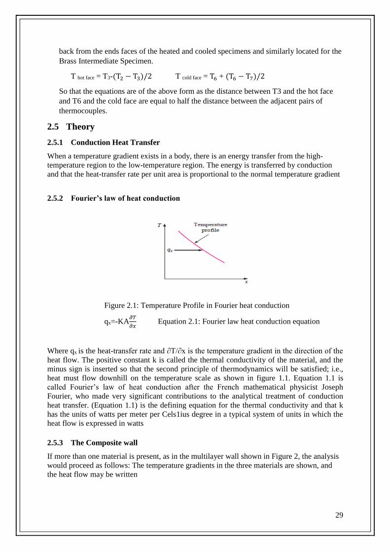
Figure 2.1: Temperature Profile in Fourier heat conduction ................................................... 29
Figure 2.2: Heat through composite wall ................................................................................. 30
Figure 2.3: Schematic diagram of experiment ........................................................................ 31
Figure 2.4: Schematic diagram of experiment ......................................................................... 33
Figure 3.1: Heat transfer through cylinder ............................................................................... 36
Figure 3.2: Temperature distribution in cylinder ..................................................................... 36
Figure 4.1: Schematic diagram of experiment ........................................................................ 42
Figure.5.1: Schematic diagram for shape factor ..................................................................... 46
Figure 5.2: Schematic diagram of experiment ........................................................................ 47
Figure 6.1: Schematic Diagram of Experiment ...................................................................... 53
Figure 7.1: Schematic Diagram of Experiment ...................................................................... 59
Figure 8.1: Schematic Diagram of Experiment ...................................................................... 68
Figure 8.1: Schematic Diagram of Experiment ...................................................................... 85
Figure 12.1: Schematic Diagram of Experiment ..................................................................... 92
Figure 13.1: Schematic Diagram of Experiment ................................................................... 103
Figure 13.2: Parallel and counter parallel flow ...................................................................... 104
Figure 13.3: Shell and tube heat exchanger ........................................................................... 104
Figure 14.1: Schematic Diagram of Experiment ................................................................... 113
Figure 14.2: Parallel and counter parallel flow ...................................................................... 114

18
List of Tables
Table 1.1: Temperatures observation at different points of specimen ..................................... 22
Table 1.2: Calculation of thermal conductivity ....................................................................... 23
Table 1.3: Distribution of temperature through uniform plane wall ........................................ 25
Table 2.1: Temperatures observation at different points of specimen ..................................... 31
Table 2.2: Calculation of overall heat transfer coefficient ...................................................... 32
Table 3.1: Distribution of temperature for different voltages .................................................. 37
Table 3.2: Thermal conductivity of given sample ................................................................... 38
Table 4.1: Measurement of temperatures from radiometer ..................................................... 43
Table 4.2: Calculation of intensity of radian ........................................................................... 44
Table 4.3: Calculation of shape factor ..................................................................................... 44
Table 5.1: Measurement of temperatures from radiometer ..................................................... 48
Table 5.2: Radiation incident on the detector .......................................................................... 49
Table 6.1: Table of Physical properties of Air at Atmospheric Pressure ................................. 51
Table 6.2: Measurement of temperature for free convection ................................................... 54
Table 6.3: Heat transfer due to free convection and radiation ................................................. 54
Table 7.1: Table of Physical properties of Air at Atmospheric Pressure ................................. 57
Table 7.2: Measurement of temperature due to forced convection ......................................... 60
Table 7.3: Heat transfer due to forced convection ................................................................... 60
Table 8.1: Temperatures measured at different distances from T1 ......................................... 68
Table 8.2: Heat transfer from extended surface ....................................................................... 69
Table 9.1: Temperatures at different points from radiant source ............................................. 73
Table 10.1: Specimen: 20mm diameter Brass Cylinder. ......................................................... 79
Table 10.2: Specimen: 20mm Stainless Steel Cylinder ........................................................... 79
Table 10.3: Properties of Specimen: 20mm diameter Brass Cylinder .................................... 80
Table 10.4: Properties of Specimen: 20mm diameter stainless steel Cylinder ....................... 80
Table 11.1: Temperatures in free convection .......................................................................... 87
Table 11.2: Temperatures in forced convection ...................................................................... 87
Table 11.3: Temperatures for different geometry of exchangers ............................................ 88
Table 12.1: Temperature at different points of turbulent flow heat exchanger ....................... 95
Table 12.2: Heat transfer calculation in turbulent flow heat exchanger .................................. 95
Table 12.3: Temperature for parallel and cross flow ............................................................... 97
Table 12.4: Effectiveness of turbulent flow exchanger ........................................................... 98
Table 13.1: Valve positions of shell and tube heat exchanger ............................................... 103
Table 13.2: Temperatures at shell and tube heat exchanger .................................................. 106
Table13.3: Heat transfer coefficient of shell and tube heat exchanger .................................. 107
Table 13.4: Temperatures for shell and tube heat exchanger ................................................ 108
Table 13.5: Effectiveness of shell and tube heat exchanger .................................................. 109
Table 14.1: Position of valves in plate heat exchanger .......................................................... 113
Table 14.2: Temperatures of Plate Heat Exchangers ............................................................. 115
Table14.3: Heat transfer in Plate heat exchanger .................................................................. 116

19
List of Graphs
Graph 7.1: Kinematic velocity of air at standard Pressure ...................................................... 63
Graph 7.2: Thermal conductivity of air at standard pressure ................................................... 64
Graph 7.3: Prandtl number of air at standard pressure ........................................................... 65
Graph 10.1: Heisler charts ....................................................................................................... 83

20
1. LAB SESSION 1
To apply Fourier Rate Equation for steady flow of heat through plane solid materials.
1.1 Learning Objectives
[i] To identify a given sample by determining its thermal conductivity.
[ii] To measure temperature distribution through a uniform plane wall and analyse the
effect of a change in heat flow.
1.2 Apparatus
Linear Heat Transfer unit H111A (Serial no H111A/04417)
1.3 Main Parts of Linear Heat Transfer Unit
1) Hydraulic Bench
2) Specimen of different materials (Brass, Aluminium, Stainless Steel)
3) Main digital Control panel (H111)
4) Temperature Sensors
1.4 Useful Data
Heated Section:
Material: Brass 25 mm diameters, Thermocouples T1, T2, T3 at 15mm spacing. Thermal
Conductivity: Approximately 121 W/mK
Cooled Section:
Material: Brass 25 mm diameters, Thermocouples T6, T7, T8 at 15mm spacing. Thermal
Conductivity: Approximately 121 W/mK
Brass Intermediate Specimen:
Material: Brass 25 mm diameters * 30mm long. Thermocouples T4, T5 at 15mm spacing
centrally spaced along the length. Thermal Conductivity: Approximately 121 W/mK
Hot and Cold Face Temperature:
Due to the need to keep the spacing of the thermocouples constant at 15mm with, or
without the intermediate specimens in position the thermocouples are displaced 7.5 mm
back from the ends faces of the heated and cooled specimens and similarly located for the
Brass Intermediate Specimen.
T hot face = T3-(T2 − T3)/2 T cold face = T6 + (T6 − T7)/2
So that the equations are of the above form as the distance between T3 and the hot face
and T6 and the cold face are equal to half the distance between the adjacent pairs of
thermocouples.
21
1.5 Theory
1.5.1 Conduction Heat Transfer
When a temperature gradient exists in a body, there is an energy transfer from the high-
temperature region to the low-temperature region. The energy is transferred by conduction
and that the heat-transfer rate per unit area is proportional to the normal temperature gradient
1.5.2 Fourier’s law of heat conduction
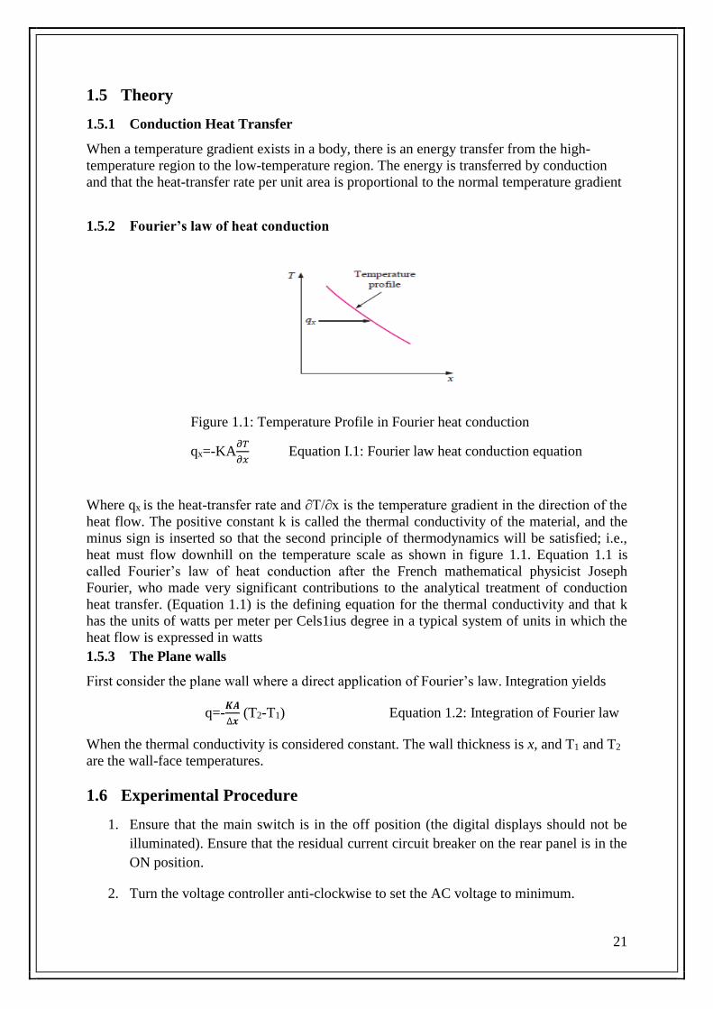
Figure 1.1: Temperature Profile in Fourier heat conduction
qx=-KA𝜕𝑇
𝜕𝑥 Equation I.1: Fourier law heat conduction equation
Where qx is the heat-transfer rate and ∂T/∂x is the temperature gradient in the direction of the
heat flow. The positive constant k is called the thermal conductivity of the material, and the
minus sign is inserted so that the second principle of thermodynamics will be satisfied; i.e.,
heat must flow downhill on the temperature scale as shown in figure 1.1. Equation 1.1 is
called Fourier’s law of heat conduction after the French mathematical physicist Joseph
Fourier, who made very significant contributions to the analytical treatment of conduction
heat transfer. (Equation 1.1) is the defining equation for the thermal conductivity and that k
has the units of watts per meter per Cels1ius degree in a typical system of units in which the
heat flow is expressed in watts
1.5.3 The Plane walls
First consider the plane wall where a direct application of Fourier’s law. Integration yields
q=-𝑲𝑨
∆𝒙 (T2-T1) Equation 1.2: Integration of Fourier law
When the thermal conductivity is considered constant. The wall thickness is x, and T1 and T2
are the wall-face temperatures.
1.6 Experimental Procedure
1. Ensure that the main switch is in the off position (the digital displays should not be
illuminated). Ensure that the residual current circuit breaker on the rear panel is in the
ON position.
2. Turn the voltage controller anti-clockwise to set the AC voltage to minimum.

22
3. Ensure the cold-water supply and electrical supply is turned on at the source. Open
the water tap until the flow through the drain hose is approximately 1.5 litters/minute.
4. Release the toggle clamp tensioning screw and clamps. Ensure that the faces of the
exposed ends of the heated and cooled sections are clean.
5. Turn on the main switch and the digital displays should illuminate. Set the
temperature selector switch to T1 to indicate the temperature of the heated end of the
bar.
6. Following the above procedure ensure cooling water is flowing and then set the heater
voltage V to approximately 150 volts. This will provide a reasonable temperature
gradient along the length of the bar. If however the local cooling water supply is at a
high temperature (25-35℃ or more) then it may be necessary to increase the voltage
supplied to the heater. This will increase the temperature difference between the hot
and cold ends of the bar.
7. Monitor temperatures T1, T2, T3, T4, T5, T6, T7, T8 until stable. When the
temperatures are stabilized record T1, T2, T3, T4, T5, T6, T7, T8, V, I
8. Increase the heater voltage by approximately 50 volts and repeat the above procedure
again recording the parameters T1, T2, T3, T4, T5, T6, T7, T8, V, I when temperature
have stabilized.
9. When the experimental procedure is completed, it is good practice to turn off the
power to the heater by reducing the voltage to zero and allow the system a short time
to cool before turning off the cooling water supply.
1.7 Observations
Sample
No.
T1
T2 T3 T4 T5 T6 T7 T8 V I
°𝑪 °𝑪 °𝑪 °𝑪 °𝑪 °𝑪 °𝑪 °𝑪 Volts Amps
1
2
3
4
Distance
from T1
0.000 0.015 0.030 0.045 0.060 0.075 0.090 0.105
Table 1.1: Temperatures observation at different points of specimen

23
1.8 Calculated Data
1.8.1 Objective:1
To identify a given sample by determining its thermal conductivity.
Figure.1.2: Schematic diagram of experiment
Specimen cross sectional Area A=0.00049m2
Specimen Length =0.030m
Sample
No.
Q̇ 𝐓𝐡𝐨𝐭𝐟𝐚𝐜𝐞 𝐓𝐜𝐨𝐥𝐝𝐟𝐚𝐜𝐞 ∆𝐓𝐢𝐧𝐭 𝐤𝐢𝐧𝐭 Material
Name
𝑾𝒂𝒕𝒕𝒔 ℃ ℃ 𝑲 𝑾/𝒎𝑲
1
2
3
4
Table 1.2: Calculation of thermal conductivity
1.8.1.1 Specimen Calculations
Intermediate Specimen and hot and cold section cross sectional Area;
A =πD2
4
Heat transfer rate from the heater;
Q̇ = V ∗ I

24
Note that the thermocouples T3 and T6 do not record the hot face and cold face temperatures,
as are both displaced by 0.0075m from T3 and T6 as shown.
Figure.1.3: Schematic diagram of experiment
If it is assumed that the temperature distribution is linear, then the actual temperature at the
hot face and cold face may be determined from the following equations.
T hot face = T3-(T2 − T3)/2
And
T cold face = T6 + (T6 − T7)/2
∆Tint = Thotface_Tcoldface
From the above parameters, the thermal conductivity of the aluminum intermediate section
may be calculated.
kint =Q̇∆xint
Aint(Thotface − Tcoldface)=
Q̇∆xint
Aint∆Tint
1.8.1.2 Graph:
Plot a graph b/w Temperature and Distance from T1 thermocouple. The thermal conductivity
of the intermediate sample may also be calculated from the data it is plotted on a graph. From
the graph the slope of the line is.
∆Tint
∆xint=X
kint =Q̇
A∗
∆Tint
∆xint
1.8.1.3 Statistical Analysis
For Thermal conductivity
% Error= 𝐾𝑡ℎ−𝐾𝑒𝑥𝑝
Kth
xavg= x1+x2+x3
n
Sx=√1
𝑛−1((𝑥1 − 𝑥𝑎𝑣𝑔)2 + (𝑥2 − 𝑥𝑎𝑣𝑔)2 + (𝑥3 − 𝑥𝑎𝑣𝑔)2)

25
1.8.1.4 Conclusion
1.8.2 Objective:2
To measure the temperature distribution through a uniform plane wall and demonstrate the effect of a
change in heat flow.
Figure 1.4: Schematic diagram of experiment
Sample
No.
�̇� ∆𝑇
1-3
∆𝑇
6-8
∆𝑥
1-3
∆𝑥
6-8
∆𝑇1−3
∆𝑥1−3
∆𝑇6−8
∆𝑥6−8 �̇�/(
∆𝑇1−3
∆𝑥1−3) �̇�/(
∆𝑇6−8
∆𝑥6−8)
W ℃ ℃ m M ℃/m ℃/m W/mK W/mK
1
2
3
4
Table 1.3: Distribution of temperature through uniform plane wall
1.8.2.1 Specimen Calculations
Heat transfer rate from the heater;
Q̇ = V ∗ I
Temperature difference in the heated section between T1 and T3;

26
∆Thot = ∆T1−3 = T1 − T3
Similarly the temperature difference in the cooled section between T6 and T8;
∆Tcold = ∆T6−8 = T6 − T8
The distance between the temperatures measuring points, T1 and T3and T6 and T8, are
similar;
∆x1−3=
∆x6−8=
Hence the temperature gradient along the heated and cooled sections may be calculated from
HeatedSection =∆T1−3
∆x1−3=
CooledSection =∆T6−8
∆x6−8=
If the constant rate of heat transfer is divided by the temperature gradients, the value obtained
will be similar if the equation is valid.
Q̇ = C∆T
∆x
Q̇
(∆T
∆x)
= C
Hence, substituting the values obtained gives for the heated section and cooled sections
respectively for following values.
Q̇
(∆T1−3
∆x1−3) =
⁄
Q̇
(∆T6−8
∆x6−8) =⁄
As may be seen from the above example and the tabulated data the function does result in a
constant value within the limits of the experimental data.
Q̇
(∆T
∆x)
= C
1.8.2.2 Statistical Analysis
For Constant “C”
% Error= 𝐾𝑡ℎ−𝐾𝑒𝑥𝑝
Kth
xavg= x1+x2+x3
n

27
Sx=√1
𝑛−1((𝑥1 − 𝑥𝑎𝑣𝑔)2 + (𝑥2 − 𝑥𝑎𝑣𝑔)2 + (𝑥3 − 𝑥𝑎𝑣𝑔)2)
1.8.2.3 Conclusion
1.9 Questions
1) What is conduction heat transfer?
2) What is Fourier law of heat conduction
3) What is meant by thermal resistance
1.10 Comments
28
2. LAB SESSION 2
To apply Fourier Rate Equation for steady flow of heat through composite plate
2.1 Learning Objective
I. To measure the temperature distribution through a composite plane wall and determine the
overall Heat Transfer Coefficient for the flow of heat through a combination of different
materials
2.2 Apparatus
Linear Heat Transfer unit H111A (Serial no H111A/04417)
2.3 Main Parts of Linear Heat Transfer Unit
5) Hydraulic Bench
6) Specimen of different materials (Brass, Aluminium, Stainless Steel)
7) Main digital Control panel (H111)
8) Temperature Sensors
2.4 Useful Data
Heated Section:
Material: Brass 25 mm diameters, Thermocouples T1, T2, T3 at 15mm spacing. Thermal
Conductivity: Approximately 121 W/mK
Cooled Section:
Material: Brass 25 mm diameters, Thermocouples T6, T7, T8 at 15mm spacing. Thermal
Conductivity: Approximately 121 W/mK
Brass Intermediate Specimen:
Material: Brass 25 mm diameters * 30mm long. Thermocouples T4, T5 at 15mm spacing
centrally spaced along the length. Thermal Conductivity: Approximately 121 W/mK
Stainless Steel Intermediate Specimen:
Material: Stainless Steel, 25 mm diameters * 30mm long. No Thermocouples fitted.
Thermal Conductivity: Approximately 25 W/mK
Aluminum Intermediate Specimen:
Material: Aluminum Alloy, 25 mm diameters * 30mm long. No Thermocouples fitted.
Thermal Conductivity: Approximately 180 W/mK
Hot and Cold Face Temperature:
Due to the need to keep the spacing of the thermocouples constant at 15mm with, or
without the intermediate specimens in position the thermocouples are displaced 7.5 mm
29
back from the ends faces of the heated and cooled specimens and similarly located for the
Brass Intermediate Specimen.
T hot face = T3-(T2 − T3)/2 T cold face = T6 + (T6 − T7)/2
So that the equations are of the above form as the distance between T3 and the hot face
and T6 and the cold face are equal to half the distance between the adjacent pairs of
thermocouples.
2.5 Theory
2.5.1 Conduction Heat Transfer
When a temperature gradient exists in a body, there is an energy transfer from the high-
temperature region to the low-temperature region. The energy is transferred by conduction
and that the heat-transfer rate per unit area is proportional to the normal temperature gradient
2.5.2 Fourier’s law of heat conduction
Figure 2.1: Temperature Profile in Fourier heat conduction
qx=-KA𝜕𝑇
𝜕𝑥 Equation 2.1: Fourier law heat conduction equation
Where qx is the heat-transfer rate and ∂T/∂x is the temperature gradient in the direction of the
heat flow. The positive constant k is called the thermal conductivity of the material, and the
minus sign is inserted so that the second principle of thermodynamics will be satisfied; i.e.,
heat must flow downhill on the temperature scale as shown in figure 1.1. Equation 1.1 is
called Fourier’s law of heat conduction after the French mathematical physicist Joseph
Fourier, who made very significant contributions to the analytical treatment of conduction
heat transfer. (Equation 1.1) is the defining equation for the thermal conductivity and that k
has the units of watts per meter per Cels1ius degree in a typical system of units in which the
heat flow is expressed in watts
2.5.3 The Composite wall
If more than one material is present, as in the multilayer wall shown in Figure 2, the analysis
would proceed as follows: The temperature gradients in the three materials are shown, and
the heat flow may be written

30
q=−kAA𝑻𝟐−𝑻𝟏
∆𝒙𝑨= −kBA
𝑻𝟑−𝑻𝟐
∆𝒙𝑩= −kCA
𝑻𝟒−𝑻𝟑
∆𝒙𝑪 Equation 2.2: Heat through composite wall
Note that the heat flow must be the same through all sections
Figure 2.2: Heat through composite wall
Solving these three equations simultaneously, the heat flow is written
q=T1−T4
∆xAkAA
+∆xB
kBAA+
∆xCkCA
Equation 2.3: Heat flow equation through composite wall
With composite systems, it is often convenient to work with an overall heat transfer
coefficient U, which is defined by an expression analogous to Newton’s law of cooling.
Accordingly
Q=UA∆T Equation 2.4: Overall heat transfer coefficient
Where ∆T is the overall temperature difference. Readers can read Further detail from book
“heat transfer by J.P Holman” in “chapter 2”
2.6 Experimental Procedure
1. Ensure that the main switch is in the off position (the digital displays should not be
illuminated). Turn the voltage controller anti-clockwise to set the AC voltage to
minimum.
2. Ensure the cold-water supply and electrical supply is turned on at the source. Open
the water tap until the flow through the drain hose is approximately 1.5 litters/minute.
3. Release the toggle clamp tensioning screw and clamps. Ensure that the faces of the
exposed ends of the heated and cooled sections are clean. Similarly, check the faces of
the Intermediate specimen to be placed between the faces of the heated and cooled
section.
4. Turn on the main switch and the digital displays should illuminate. Set the
temperature selector switch to T1 to indicate the temperature of the heated end of the
bar.
5. Following the above procedure ensure cooling water is flowing and then set the heater
voltage V to approximately 150 volts. This will provide a reasonable temperature

31
gradient along the length of the bar. If, however the local cooling water supply is at a
high temperature (25-35℃ or more) then it may be necessary to increase the voltage
supplied to the heater. This will increase the temperature difference between the hot
and cold ends of the bar.
6. Monitor temperatures T1, T2, T3, T4, T5, T6, T7, T8 until stable.
7. Increase the heater voltage by approximately 50 volts and repeat the above procedure
again recording the parameters T1, T2, T3, T4, T5, T6, T7, T8, V, I when temperature
have stabilized.
2.7 Observations
Sample
No.
T1
T2 T3 T4 T5 T6 T7 T8 V I
°𝑪 °𝑪 °𝑪 °𝑪 °𝑪 °𝑪 °𝑪 °𝑪 Volts Amps
1
2
3
4
Distance
from T1
0.000 0.015 0.030 0.045 0.060 0.075 0.090 0.105
Table 2.1: Temperatures observation at different points of specimen
To measure the temperature distribution through a composite plane wall and determine the overall
Heat Transfer Coefficient for the flow of heat through a combination of different materials in use.
Figure 2.3: Schematic diagram of experiment

32
Specimen cross sectional Area A = 0.00049m2
Conductivity of Brass heated and cooled section =121𝑊/𝑚𝐾
Conductivity of Stainless steel intermediate section =25𝑊/𝑚𝐾
Sample
No.
Q ∆T1−8 ∆xhot ∆xint ∆xcold khot kint kcold
-- W K m M m 𝑊𝑚𝐾⁄ 𝑊
𝑚𝐾⁄ 𝑊𝑚𝐾⁄
1
2
3
4
Table 2.2: Calculation of overall heat transfer coefficient
2.7.1.1 Specimen Calculations
Brass Intermediate Specimen and hot and cold section cross sectional Area;
A =πD2
4
The temperature difference across the bar from T1 to T8;
T1 − T8 =X
Note that ∆𝑥ℎ𝑜𝑡 and ∆𝑥𝑐𝑜𝑙𝑑are the distances between the thermocouple T1 and the hot face
and the cold face and the thermocouple T8 respectively. Similarly, ∆𝑥𝑖𝑛𝑡 is the distance
between the hot face and cold face of the intermediate stainless steel section.
Sample No. U =
1
(xhot
khot+
xint
kint+
xcold
kcold)
Q
𝐴(T1 − T8)= U
-- 𝑊
𝑚2𝐾
𝑊
𝑚2𝐾
1
2
3
4

33
Figure 2.4: Schematic diagram of experiment
The distances between surfaces are therefore as follows.
∆xhot = 0.0375m
∆xint = 0.030m
∆xcold = 0.0375m
Heat transfer rate from the heater;
Q = VI
Hence
U =Q
A(T1 − T8)
Similarly,
U =1
(xhot
khot+
xint
kint+
xcold
kcold)
Note that the U value resulting from the test data differs from that resulting from assumed
thermal conductivity and material thickness. This is most likely due to un-accounted for heat
losses and thermal resistances between the hot face interface and cold face inter face with the
stainless steel intermediate section.
2.7.1.2 Graph
Plot a graph b/w Temperature and Distance from T1 thermocouple. The temperature data may
be plotted against position along the bar and straight lines drawn through the temperature
points for the heated and cooled sections. Then a straight line may be drawn through the hot

34
face and cold face temperature to extrapolate the temperature distribution in the stainless steel
intermediate section.
2.7.1.3 Statistical Analysis
For Constant “U”
% Error= 𝐾𝑡ℎ−𝐾𝑒𝑥𝑝
Kth
xavg= x1+x2+x3
n
Sx=√1
𝑛−1((𝑥1 − 𝑥𝑎𝑣𝑔)2 + (𝑥2 − 𝑥𝑎𝑣𝑔)2 + (𝑥3 − 𝑥𝑎𝑣𝑔)2)
2.7.1.4 Conclusion
2.8 Questions
1) Define Overall heat transfer coefficient
2) Define thermal conductivity and explain its significance in heat transfer.
2.9 Comments
35
3. LAB SESSION NO 03
To apply the Fourier Rate Equation for steady flow of heat through cylindrical solid materials
3.1 Learning Objective
[i] To identify a given sample (disc material) by determining its thermal conductivity.
3.2 Apparatus
Radial Heat Transfer unit H111B
3.3 Main Parts of Radial Heat transfer unit
1) Hydraulic Bench
2) Specimen of different materials
3) Main digital Control panel (H111)
4) Temperature Sensors
3.4 Useful Data
3.4.1 Radial Heat Conduction
3.4.2 Heated disc:
Material: Outside Diameter: 0.110m
Diameter of Heated Sample Core: 0.014m
Thickness of Disc (x): 0.0032m
Radial Position of Thermocouples:
T1=0.007m
T2=0.010m
T3=0.020m
T4=0.030m
3.5 Theory
3.5.1 Conduction Heat Transfer
When a temperature gradient exists in a body, there is an energy transfer from the high-
temperature region to the low-temperature region. The energy is transferred by conduction
and that the heat-transfer rate per unit area is proportional to the normal temperature gradient.
3.5.2 Radial Systems
3.5.2.1 Cylinders
Consider a long cylinder of inside radius ri, outside radius ro, and length L, such as the one
shown in Figure 2.1.We expose this cylinder to a temperature differential Ti −To. For a

36
cylinder with length very large compared to diameter, it may be assumed that the heat flows
only in a radial direction, so that the only space coordinate needed to specify the system is r.
Again, Fourier’s law is used by inserting the proper area relation. The area for heat flow in
the cylindrical system is
Ar =2πrL
So that Fourier’s law is written
qr= −kAr dT
dr
qr= −2πkrL dT
dr Equation 3.1: Fourier Law equation for cylinders
Figure 3.1: Heat transfer through cylinder
Figure 3.2: Temperature distribution in cylinder
With the boundary conditions
T=Ti at r=ri
T=T0 at r=r0
The solution to Equation 3.1 is
q=2πkL(Ti−T°)
ln (r°ri
) Equation 3.2: Fourier Law equation for cylinders
3.6 Procedure
1. Ensure that the main switch is in the off position (the digital displays should not be
illuminated).

37
2. Ensure the cold water supply and electrical supply is turned on at the source. Open
the water tap until the flow through the drain hose is approximately 1.5 liters/minute.
3. Turn on the main switch and the digital displays should illuminate. Set the
temperature selector switch to T1 to indicate the temperature of the heated centre of
the disc.
4. Following the above procedure ensure cooling water is flowing and then set the
heater voltage V to approximately 50 volts.
5. Monitor temperatures T1, T2, T3, T4, T5, and T6 until stable. When the
temperatures are stabilized record: T1, T2, T3, T4, T5, T6, V, I
6. Reset heater voltage to 100 volts and repeat the above procedure again and Monitor
temperatures T1, T2, T3, T4, T5, and T6 until stable. When the temperatures are
stabilized record: T1, T2, T3, T4, T5, T6 V, I. Repeat procedure with the difference of
50 V voltage
3.7 Observations
Sample
No.
T1 T2 T3 T4 T5 T6 V I
⁰C ⁰C ⁰C ⁰C ⁰C ⁰C Volts Amps
1
2
3
4
Radius
0.007 0.010 0.020 0.030 0.040 0.050 --- ---
Table 3.1: Distribution of temperature for different voltages
3.8 Calculated Data
3.8.1 Objective
To identify a given sample (disc material) by determining its thermal conductivity.
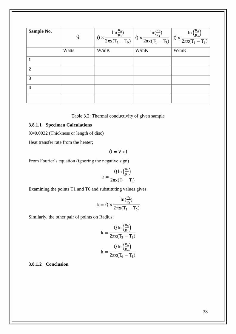
38
Sample No. Q̇ Q̇ ×
ln(R6
R1)
2πx(T1 − T6) Q̇ ×
ln(R3
R1)
2πx(T1 − T3) Q̇ ×
ln (R6
R4)
2πx(T4 − T6)
Watts W/mK W/mK W/mK
1
2
3
4
Table 3.2: Thermal conductivity of given sample
3.8.1.1 Specimen Calculations
X=0.0032 (Thickness or length of disc)
Heat transfer rate from the heater;
Q̇ = V ∗ I
From Fourier’s equation (ignoring the negative sign)
k =Q̇ ln (
R°
Ri)
2πx(T° − Ti)
Examining the points T1 and T6 and substituting values gives
k = Q̇ ×ln(
R6
R1)
2πx(T1 − T6)
Similarly, the other pair of points on Radius;
k =Q̇ ln (
R3
R1)
2πx(T3 − T1)
k =Q̇ ln (
R6
R4)
2πx(T6 − T4)
3.8.1.2 Conclusion
39
3.8.1.3 Graph
Plot a graph b/w Radius from heated disc centre (x-axis) and Temperature (y-axis).
3.9 Statistical Analysis
For Thermal conductivity
% Error= 𝐾𝑡ℎ−𝐾𝑒𝑥𝑝
Kth
xavg= x1+x2+x3
n
Sx=√1
𝑛−1((𝑥1 − 𝑥𝑎𝑣𝑔)2 + (𝑥2 − 𝑥𝑎𝑣𝑔)2 + (𝑥3 − 𝑥𝑎𝑣𝑔)2)
3.10 Questions
1) How temperature distribution through the wall of a thick cylinder
2) What is steady-state heat transfer?
3) What is effect of changing the thickness of cylinder on thermal conductivity?
4) Why by increasing input heat Q, overall slope of the temperature gradients increases.
3.11 Comments

40
4. LAB SESSION 4
To verify laws of radiation by using shape factor
4.1 Learning Objectives
To verify the inverse square law for thermal radiation
To verify the Stefan Boltzmann Law
4.2 Apparatus
Radiation Heat Transfer unit H111C (Serial no H111C/01310)
4.3 Main Parts
1) Heat Source
2) Radiation detector
3) Temperature Sensors
4) Radiometer output unit
5) Main digital Control panel (H111)
4.4 Useful Data
Laws of radiant heat transfer and radiant heat exchange (H111C)
Stefen-Boltzman Constant σ =5.67𝑥10−8 w
m2k4
4.5 Theory
4.5.1 Radiation
Radiation is the emission or transmission of energy in the form of waves or particles through
space or through a material medium.
4.5.2 Radiation Heat Transfer
Thermal radiation is electromagnetic radiation generated by the thermal motion of charged
particles in matter. All matter with a temperature greater than absolute zero emits thermal
radiation. When the temperature of the body is greater than absolute zero, interatomic
collisions cause the kinetic energy of the atoms or molecules to change. All bodies radiate
energy in the form of photons moving in a random direction, with random phase and
frequency. When radiated photons reach another surface, they may be absorbed, reflected or
transmitted. The behavior of a surface with radiation incident upon it can be described by the
following quantities:
= absorptance =fraction of incident radiation absorbed
Ρ= reflectance = fraction of incident radiation reflected
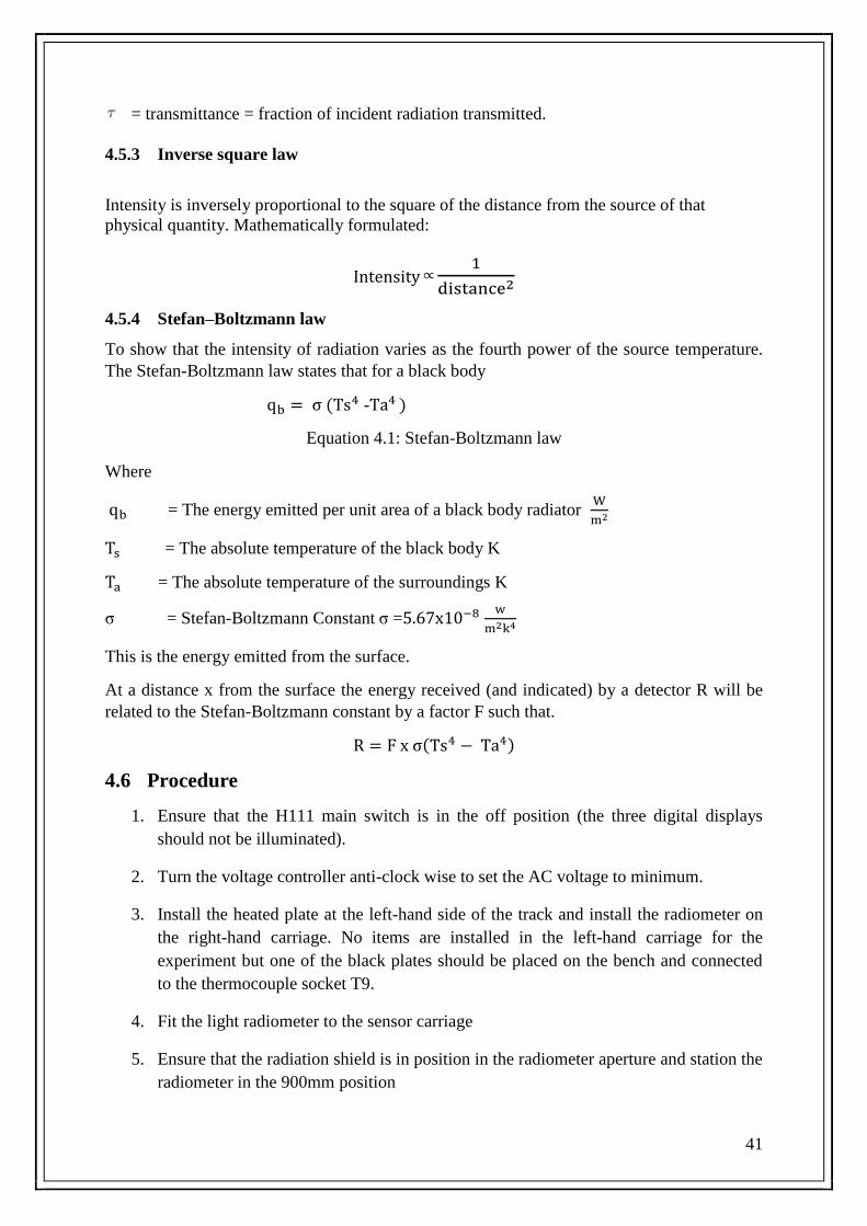
41
= transmittance = fraction of incident radiation transmitted.
4.5.3 Inverse square law
Intensity is inversely proportional to the square of the distance from the source of that
physical quantity. Mathematically formulated:
Intensity∝1
distance2
4.5.4 Stefan–Boltzmann law
To show that the intensity of radiation varies as the fourth power of the source temperature.
The Stefan-Boltzmann law states that for a black body
qb = σ (Ts4 -Ta4 )
Equation 4.1: Stefan-Boltzmann law
Where
qb = The energy emitted per unit area of a black body radiator W
m2
Ts = The absolute temperature of the black body K
Ta = The absolute temperature of the surroundings K
σ = Stefan-Boltzmann Constant σ =5.67x10⁻⁸ w
m2k4
This is the energy emitted from the surface.
At a distance x from the surface the energy received (and indicated) by a detector R will be
related to the Stefan-Boltzmann constant by a factor F such that.
R = F x σ(Ts4 − Ta4)
4.6 Procedure
1. Ensure that the H111 main switch is in the off position (the three digital displays
should not be illuminated).
2. Turn the voltage controller anti-clock wise to set the AC voltage to minimum.
3. Install the heated plate at the left-hand side of the track and install the radiometer on
the right-hand carriage. No items are installed in the left-hand carriage for the
experiment but one of the black plates should be placed on the bench and connected
to the thermocouple socket T9.
4. Fit the light radiometer to the sensor carriage
5. Ensure that the radiation shield is in position in the radiometer aperture and station the
radiometer in the 900mm position
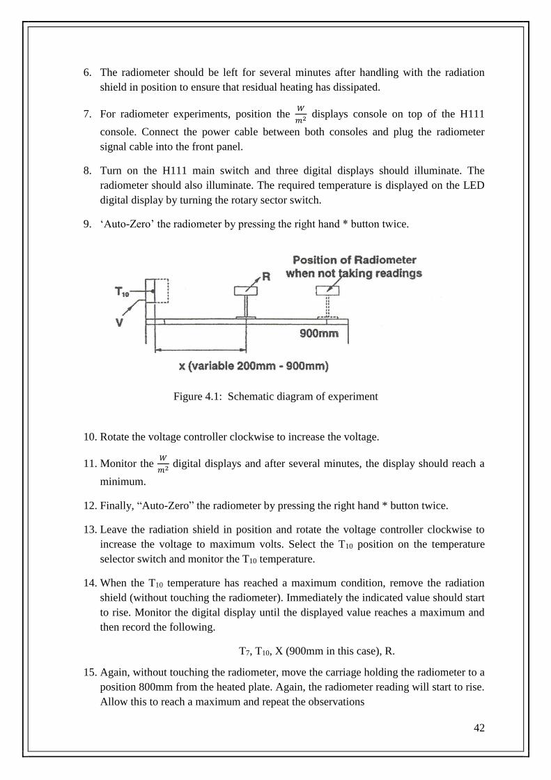
42
6. The radiometer should be left for several minutes after handling with the radiation
shield in position to ensure that residual heating has dissipated.
7. For radiometer experiments, position the 𝑊
𝑚2 displays console on top of the H111
console. Connect the power cable between both consoles and plug the radiometer
signal cable into the front panel.
8. Turn on the H111 main switch and three digital displays should illuminate. The
radiometer should also illuminate. The required temperature is displayed on the LED
digital display by turning the rotary sector switch.
9. ‘Auto-Zero’ the radiometer by pressing the right hand * button twice.
Figure 4.1: Schematic diagram of experiment
10. Rotate the voltage controller clockwise to increase the voltage.
11. Monitor the 𝑊
𝑚2 digital displays and after several minutes, the display should reach a
minimum.
12. Finally, “Auto-Zero” the radiometer by pressing the right hand * button twice.
13. Leave the radiation shield in position and rotate the voltage controller clockwise to
increase the voltage to maximum volts. Select the T10 position on the temperature
selector switch and monitor the T10 temperature.
14. When the T10 temperature has reached a maximum condition, remove the radiation
shield (without touching the radiometer). Immediately the indicated value should start
to rise. Monitor the digital display until the displayed value reaches a maximum and
then record the following.
T7, T10, X (900mm in this case), R.
15. Again, without touching the radiometer, move the carriage holding the radiometer to a
position 800mm from the heated plate. Again, the radiometer reading will start to rise.
Allow this to reach a maximum and repeat the observations

43
T7, T10, X (800mm in this case), R.
16. Repeat the above procedure in reducing steps of 100mm until the radiometer is
200mm from the heated plate.
4.7 Observations:
Sample test results
For the unit tested C = 0.786
Table 4.1: Measurement of temperatures from radiometer
While
T7= Temperature of black body
T10= Temperature of heater
X=Distance of radiometer from heater
V= Voltage
I= Current
R= Reading of radiometer in 𝑊
𝑚2
Rc= Corrected radiometer reading=Rc = R × C
4.8 Calculated Data
4.8.1 Objective:01
To verify the inverse square law for thermal radiation
V I T7 T10 x R 𝑹𝒄
900
800
700
600
500
400
300
200
𝐑𝐜 x Log10 x Log10𝐑𝐜
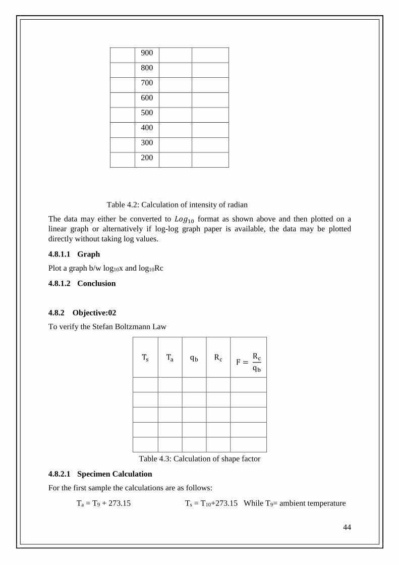
44
Table 4.2: Calculation of intensity of radian
The data may either be converted to 𝐿𝑜𝑔10 format as shown above and then plotted on a
linear graph or alternatively if log-log graph paper is available, the data may be plotted
directly without taking log values.
4.8.1.1 Graph
Plot a graph b/w log10x and log10Rc
4.8.1.2 Conclusion
4.8.2 Objective:02
To verify the Stefan Boltzmann Law
Ts
Ta
qb
Rc
F = Rc
qb
Table 4.3: Calculation of shape factor
4.8.2.1 Specimen Calculation
For the first sample the calculations are as follows:
Ta = T9 + 273.15 Ts = T10+273.15 While T9= ambient temperature
900
800
700
600
500
400
300
200
45
Hence qb = σ (Ts4 -Ta4 )
From the radiometer reading:
Rc= C x R (W
m2)
Hence F = Rc
qb
It may be seen from the test results that the factor F remains essentially constant thereby
demonstrating that the Steffen-Boltzmann relationship applies.
4.8.2.2 Conclusion
4.9 Statistical Analysis
For Shape Factor F
xavg= x1+x2+x3
n
Sx=√1
𝑛−1((𝑥1 − 𝑥𝑎𝑣𝑔)2 + (𝑥2 − 𝑥𝑎𝑣𝑔)2 + (𝑥3 − 𝑥𝑎𝑣𝑔)2
4.10 Questions
1) What is value of Log10 x corresponding to the value of 550 mm, Calculate from graph
2) How does thermal radiation differ from other types of electromagnetic radiation?
3) What is inverse square law for thermal radiation
4) Define absorptivity, reflectivity and transmissivity
5) What is the Stefan-Boltzmann law?
4.11 Comments
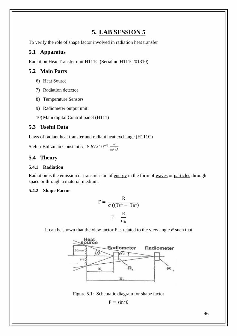
46
5. LAB SESSION 5
To verify the role of shape factor involved in radiation heat transfer
5.1 Apparatus
Radiation Heat Transfer unit H111C (Serial no H111C/01310)
5.2 Main Parts
6) Heat Source
7) Radiation detector
8) Temperature Sensors
9) Radiometer output unit
10) Main digital Control panel (H111)
5.3 Useful Data
Laws of radiant heat transfer and radiant heat exchange (H111C)
Stefen-Boltzman Constant σ =5.67𝑥10−8 w
m2k4
5.4 Theory
5.4.1 Radiation
Radiation is the emission or transmission of energy in the form of waves or particles through
space or through a material medium.
5.4.2 Shape Factor
F = R
σ ((Ts4 − Ta4)
F = R
qb
It can be shown that the view factor F is related to the view angle 𝜃 such that
Figure.5.1: Schematic diagram for shape factor
F = sin2θ
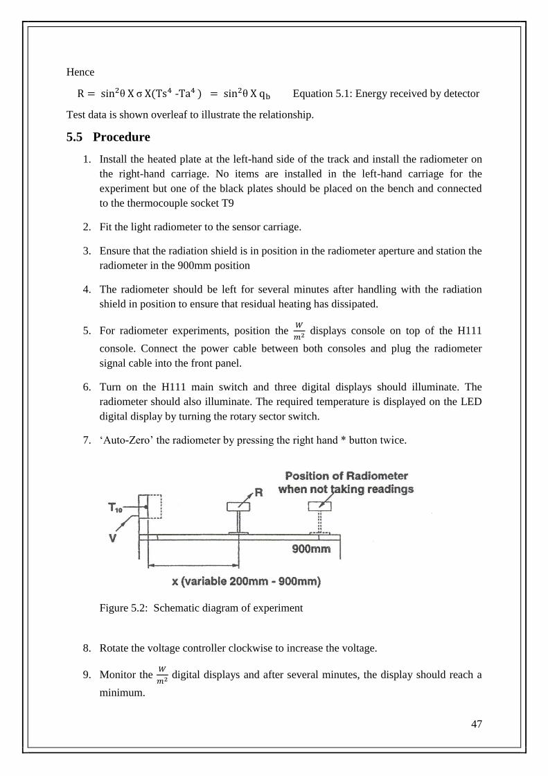
47
Hence
R = sin2θ X σ X(Ts4 -Ta4 ) = sin2θ X qb Equation 5.1: Energy received by detector
Test data is shown overleaf to illustrate the relationship.
5.5 Procedure
1. Install the heated plate at the left-hand side of the track and install the radiometer on
the right-hand carriage. No items are installed in the left-hand carriage for the
experiment but one of the black plates should be placed on the bench and connected
to the thermocouple socket T9
2. Fit the light radiometer to the sensor carriage.
3. Ensure that the radiation shield is in position in the radiometer aperture and station the
radiometer in the 900mm position
4. The radiometer should be left for several minutes after handling with the radiation
shield in position to ensure that residual heating has dissipated.
5. For radiometer experiments, position the 𝑊
𝑚2 displays console on top of the H111
console. Connect the power cable between both consoles and plug the radiometer
signal cable into the front panel.
6. Turn on the H111 main switch and three digital displays should illuminate. The
radiometer should also illuminate. The required temperature is displayed on the LED
digital display by turning the rotary sector switch.
7. ‘Auto-Zero’ the radiometer by pressing the right hand * button twice.
Figure 5.2: Schematic diagram of experiment
8. Rotate the voltage controller clockwise to increase the voltage.
9. Monitor the 𝑊
𝑚2 digital displays and after several minutes, the display should reach a
minimum.
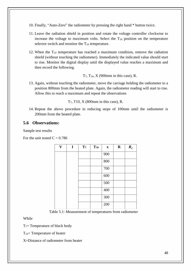
48
10. Finally, “Auto-Zero” the radiometer by pressing the right hand * button twice.
11. Leave the radiation shield in position and rotate the voltage controller clockwise to
increase the voltage to maximum volts. Select the T10 position on the temperature
selector switch and monitor the T10 temperature.
12. When the T10 temperature has reached a maximum condition, remove the radiation
shield (without touching the radiometer). Immediately the indicated value should start
to rise. Monitor the digital display until the displayed value reaches a maximum and
then record the following.
T7, T10, X (900mm in this case), R.
13. Again, without touching the radiometer, move the carriage holding the radiometer to a
position 800mm from the heated plate. Again, the radiometer reading will start to rise.
Allow this to reach a maximum and repeat the observations
T7, T10, X (800mm in this case), R.
14. Repeat the above procedure in reducing steps of 100mm until the radiometer is
200mm from the heated plate.
5.6 Observations:
Sample test results
For the unit tested C = 0.786
Table 5.1: Measurement of temperatures from radiometer
While
T7= Temperature of black body
T10= Temperature of heater
X=Distance of radiometer from heater
V I T7 T10 x R 𝑹𝒄
900
800
700
600
500
400
300
200

49
V= Voltage
I= Current
R= Reading of radiometer in 𝑊
𝑚2
Rc= Corrected radiometer reading=Rc = R × C
5.6.1 Calculated Data
Table 5.2: Radiation incident on the detector
5.6.1.1 Specimen Calculation
For the first data point at x = 900mm
Ts = T10+273.15 Ta = T9+273.15
Hence qb = σ (Ts4 − Ta
4)
From the geometry θ = tan−1(50
900)
Hence sin2θ =
From this data Rc= qb. sin2θ
The corrected radiation 𝑅𝑐 recorded by the radiometer under these conditions was
Rc = ( ) W
m2
Ts Ta qb θ sin2θ Rc = qb x sin2θ
(Theoretical)
Rc
(Experimental)
K K W
m2
Radians W
m2
W
m2

50
Comparing the calculated radiation incident on the detector 𝑞𝑏 𝑥 𝑠𝑖𝑛2𝜃 and the corrected
radiation measured by the detector 𝑅𝑐 it may be seen that the value are similar.
Note that small errors in temperature measurement affect the data to the fourth power i.e. T4
5.6.1.2 Conclusion
5.7 Statistical Analysis
NA
5.8 Questions
1) What is a gray body
2) What is meant by the radiation shape factor?
3) What is radiation shields and its effect
5.9 Comments
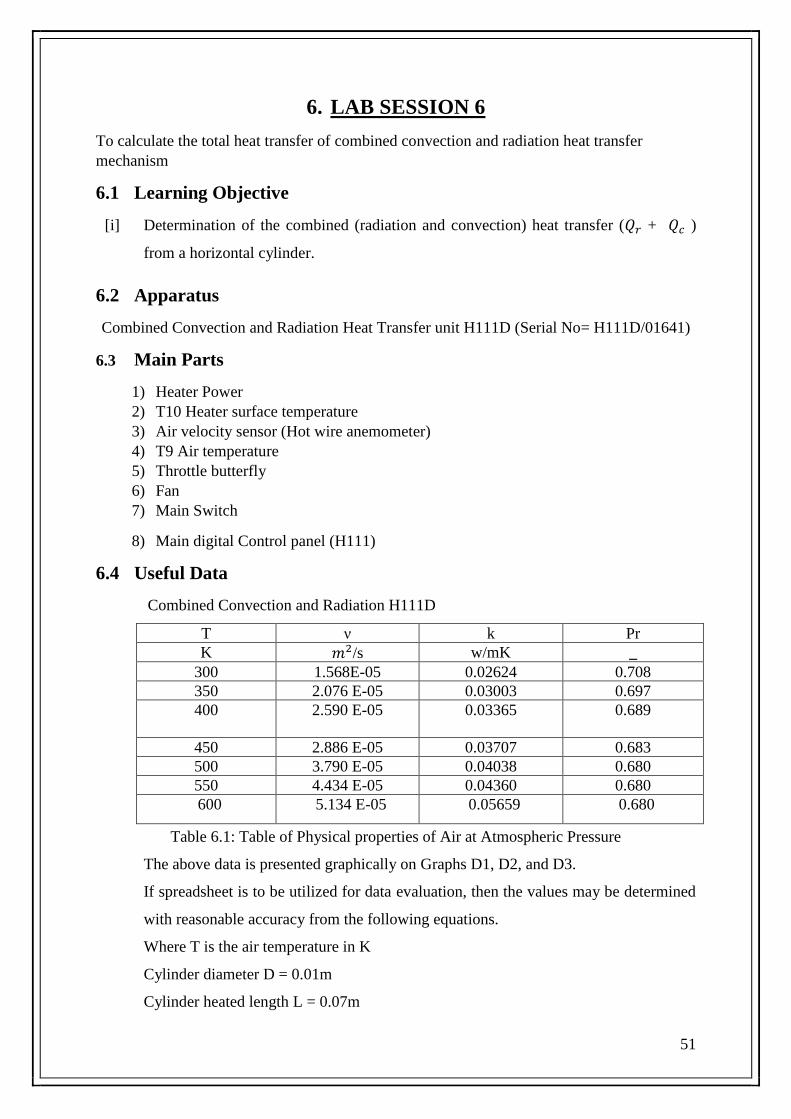
51
6. LAB SESSION 6
To calculate the total heat transfer of combined convection and radiation heat transfer
mechanism
6.1 Learning Objective
[i] Determination of the combined (radiation and convection) heat transfer (𝑄𝑟 + 𝑄𝑐 )
from a horizontal cylinder.
6.2 Apparatus
Combined Convection and Radiation Heat Transfer unit H111D (Serial No= H111D/01641)
6.3 Main Parts
1) Heater Power
2) T10 Heater surface temperature
3) Air velocity sensor (Hot wire anemometer)
4) T9 Air temperature
5) Throttle butterfly
6) Fan
7) Main Switch
8) Main digital Control panel (H111)
6.4 Useful Data
Combined Convection and Radiation H111D
T ν k Pr
K 𝑚2/s w/mK _
300 1.568E-05 0.02624 0.708
350 2.076 E-05 0.03003 0.697
400
2.590 E-05 0.03365 0.689
450 2.886 E-05 0.03707 0.683
500 3.790 E-05 0.04038 0.680
550 4.434 E-05 0.04360 0.680
600 5.134 E-05 0.05659 0.680
Table 6.1: Table of Physical properties of Air at Atmospheric Pressure
The above data is presented graphically on Graphs D1, D2, and D3.
If spreadsheet is to be utilized for data evaluation, then the values may be determined
with reasonable accuracy from the following equations.
Where T is the air temperature in K
Cylinder diameter D = 0.01m
Cylinder heated length L = 0.07m

52
Cylinder effective heated area As = 0.0022m2
Effective air velocity local to cylinder due to blockage effect Ue = Ua X 1.22
6.5 Theory
When a horizontal cylinder, with its surface at a temperature above that of its surroundings, is
located in stationary air, the heat loss from the cylinder will be a combination of natural
convection to the air (air surrounding the cylinder becomes less dense and rises when it is
heated) and radiation to the surroundings.
Heat loss due to conduction is minimized by the design of the equipment and measurements
mid-way along the heated section of the cylinder can be assumed to be unaffected by
conduction at the ends of the cylinder. Heat loss by conduction would normally be included
in the analysis of a real application.
The following theoretical analysis uses an empirical relationship for the heat transfer due to
natural convection proposed by WH McAdams in the publication "Heat Transmission", third
edition, McGraw-Hill, New York, 1959.
Total heat loss from the cylinder: Qtotal = Qc + Qr
Equation 6.1
Heat loss due to natural convection: Qc = hc As (Ts - Ta)
Equation 6.2
Heat loss due to radiation: Qr = hr As (Ts - Ta)
Equation 6.3
Heat transfer area (surface area): As = (π D L)
Equation 6.4
The heat transfer coefficients hc and hr can be calculated using the following relationships
hc=1.32 [Ts−Ta
D]
0.25
Equation 6.5
hr=ϵϭ (Ts
4−Ta4)
(Ts−Ta) Equation 6.6
ϭ= Stefan Boltzmann constant
Є = Emissivity of surface (dimensionless)
Ts = Surface temperature of cylinder (K)
Ta = Ambient temperature (K)
6.6 Procedure
1. Turn the voltage controller anti-clock wise to set the AC voltage to minimum. Ensure
the Combined Convection and Radiation H111D accessory has been connected to the
Heat Transfer Service Unit H111.
2. Ensure that the heated cylinder is located in its holder at the top of the duct and that
the cylinder is rotated so that the thermocouple location is on the side of the cylinder.
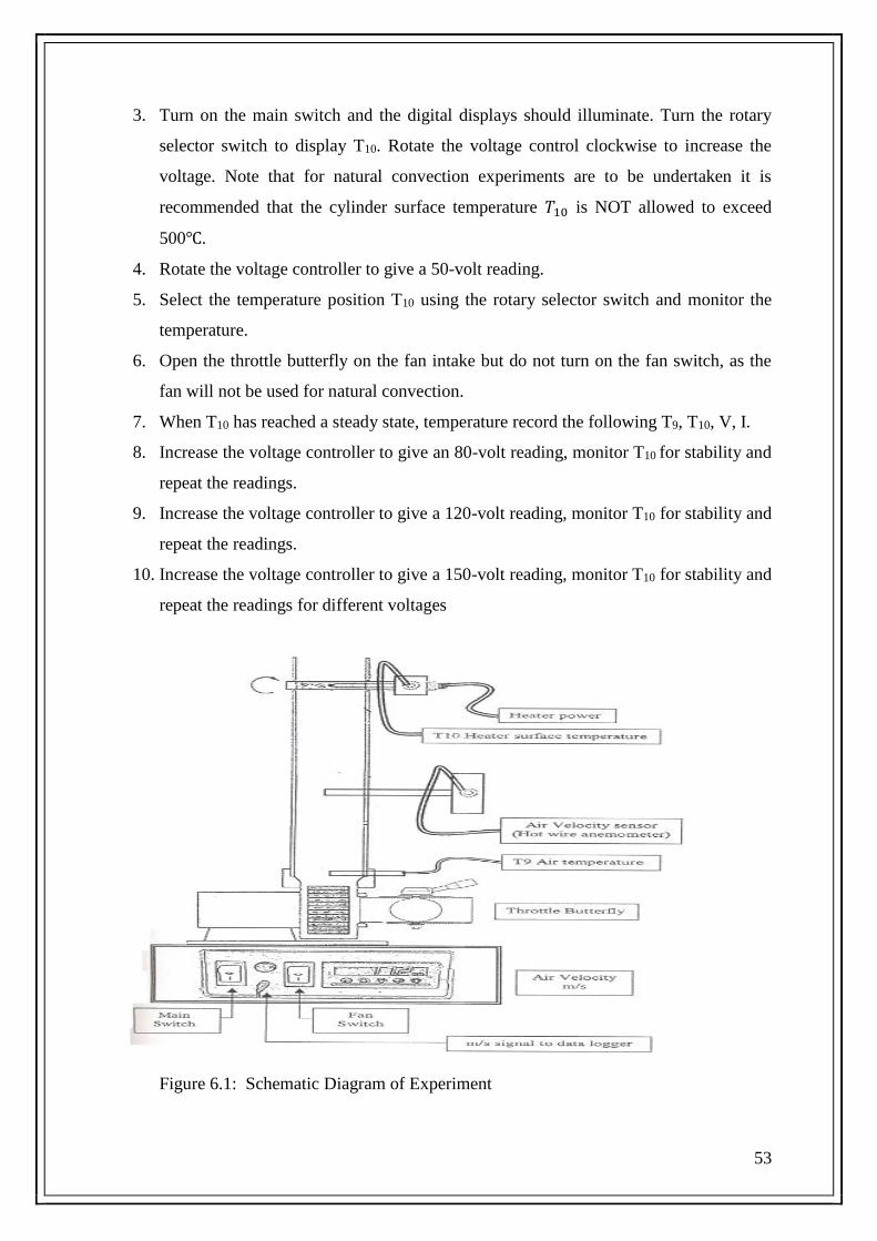
53
3. Turn on the main switch and the digital displays should illuminate. Turn the rotary
selector switch to display T10. Rotate the voltage control clockwise to increase the
voltage. Note that for natural convection experiments are to be undertaken it is
recommended that the cylinder surface temperature 𝑇10 is NOT allowed to exceed
500℃.
4. Rotate the voltage controller to give a 50-volt reading.
5. Select the temperature position T10 using the rotary selector switch and monitor the
temperature.
6. Open the throttle butterfly on the fan intake but do not turn on the fan switch, as the
fan will not be used for natural convection.
7. When T10 has reached a steady state, temperature record the following T9, T10, V, I.
8. Increase the voltage controller to give an 80-volt reading, monitor T10 for stability and
repeat the readings.
9. Increase the voltage controller to give a 120-volt reading, monitor T10 for stability and
repeat the readings.
10. Increase the voltage controller to give a 150-volt reading, monitor T10 for stability and
repeat the readings for different voltages
Figure 6.1: Schematic Diagram of Experiment

54
6.7 Calculated Data
6.7.1 Objective:01
Determination of the combined (radiation and convection) heat transfer (𝐐𝐫 + 𝐐𝐜 ) from a
horizontal cylinder.
6.7.1.1 Observations
Sample test results
Sample V I T9 T10
- Volts Amps ℃ ℃
1
2
3
4
5
Table 6.2: Measurement of temperature for free convection
T9= Ambient Temperature
T10= Heater temperature
V= Input voltage
I= Input current
Sample Qinput hr hc Qr Qc Qtot
- W W
m2k
W
m2k
W W W
1
2
3
4
5
Table 6.3: Heat transfer due to free convection and radiation
6.7.1.2 Specimen Calculations
For the first sample the calculation are as follows:
Qinput =V I
For the radiant component;
hr = εF σ(Ts
4 − Ta4)
(Ts − Ta)
Ts = T 10 + 273.15 (K)
Ta = T9 + 273.15 (K)

55
hr =0.95 X 1 X 5.67 X 10−8 (Ts
4 − Ta4)
(Ts − Ta)
= 𝑊
𝑚2𝑘
Hence the heat lost to radiation Qr
(As is obtained from USEFUL DATA on)
Qr = hrAs (Ts − Ta)
For the convective component using the simple formula
hc = 1.32 [Ts − Ta
D]
0.25
= W
m2k
Hence the heat lost to convection;
(As Is obtained from USEFUL DATA)
Qc = hcAs (Ts-Ta)
Hence the total heat lost by calculation
Qtot = Qr + Qc = (W)
In addition it may be seen that at low temperatures the convective component of heat transfer
is predominant while at higher temperatures the radiant component becomes predominant.
The temperature, at which the conditions reverse, is also influenced by the emissivity of the
surface, and that of the surroundings.
6.7.1.3 Graph
Draw the Graph of hc, hr (y-Axis) and surface Temperature T10(X- Axis)
6.7.1.4 Conclusion
56
6.8 Statistical Analysis
For total heat transfer in free convection
xavg= x1+x2+x3
n
Sx=√1
𝑛−1((𝑥1 − 𝑥𝑎𝑣𝑔)2 + (𝑥2 − 𝑥𝑎𝑣𝑔)2 + (𝑥3 − 𝑥𝑎𝑣𝑔)2)
6.9 Questions
1) Write about the trend of convective heat transfer coefficient with heater temperature
2) What is value of heater temperature at air velocity of 2.3 m/s, compute it from graph.
3) Write about the trend of Radiant heat transfer coefficient with heater temperature
6.10 Comments
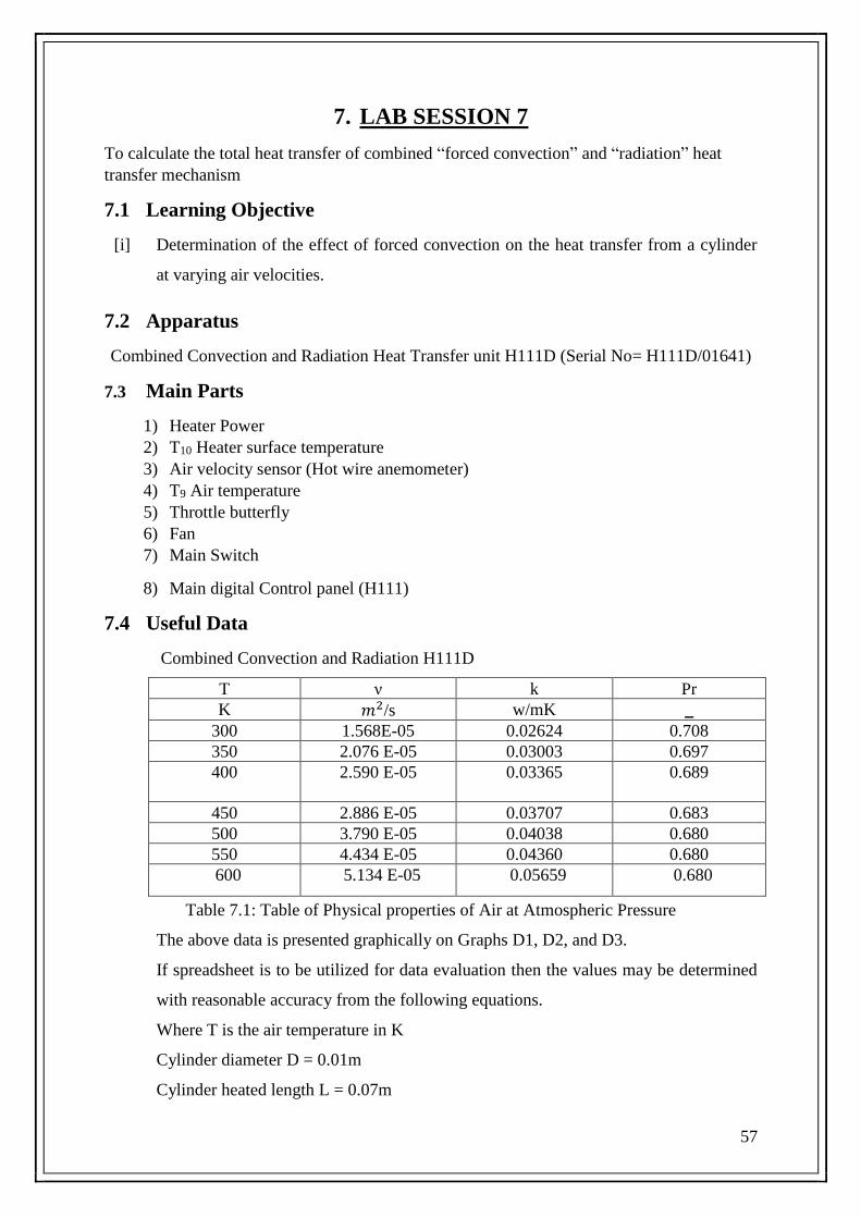
57
7. LAB SESSION 7
To calculate the total heat transfer of combined “forced convection” and “radiation” heat
transfer mechanism
7.1 Learning Objective
[i] Determination of the effect of forced convection on the heat transfer from a cylinder
at varying air velocities.
7.2 Apparatus
Combined Convection and Radiation Heat Transfer unit H111D (Serial No= H111D/01641)
7.3 Main Parts
1) Heater Power
2) T10 Heater surface temperature
3) Air velocity sensor (Hot wire anemometer)
4) T9 Air temperature
5) Throttle butterfly
6) Fan
7) Main Switch
8) Main digital Control panel (H111)
7.4 Useful Data
Combined Convection and Radiation H111D
T ν k Pr
K 𝑚2/s w/mK _
300 1.568E-05 0.02624 0.708
350 2.076 E-05 0.03003 0.697
400
2.590 E-05 0.03365 0.689
450 2.886 E-05 0.03707 0.683
500 3.790 E-05 0.04038 0.680
550 4.434 E-05 0.04360 0.680
600 5.134 E-05 0.05659 0.680
Table 7.1: Table of Physical properties of Air at Atmospheric Pressure
The above data is presented graphically on Graphs D1, D2, and D3.
If spreadsheet is to be utilized for data evaluation then the values may be determined
with reasonable accuracy from the following equations.
Where T is the air temperature in K
Cylinder diameter D = 0.01m
Cylinder heated length L = 0.07m
58
Cylinder effective heated area As = 0.0022m2
Effective air velocity local to cylinder due to blockage effect Ue = Ua X 1.22
7.5 Theory
7.5.1 Forced convection
Forced convection is a mechanism, or type of transport in which fluid motion is generated by
an external source (like a pump, fan, suction device, etc.). It should be considered as one of
the main methods of useful heat transfer as significant amounts of heat energy can be
transported very efficiently.
Actual power supplied to the heated cylinder Qin = V I (Watts) Equation 7.1
Qr = hr As (Ts - Ta)
So Nusselt number is
Nu = 0.3 + [{(0.62Re0.5Pr0.33)/(1 + (0.4
Pr)
0.66 )
0.25
} ∗ (1 + (Re
282000)
0.5) ]
Equation 7.2
And Reynolds number is
Re = UeD/v Equation 7.3
hf =k
DNu Equation 7.4
This results in a convective heat transfer of
Qf = hfAs(Ts − Ta) Equation 7.5
Hence the total heat transfer from the cylinder
Qtotal = (Qr + Qf ) Equation 7.6
7.6 Procedure
1. Ensure that the heated cylinder is located in its holder at the top of the duct and that
the cylinder is rotated so that the thermocouple location is on the side of the cylinder.
This is shown schematically below.
2. Turn on the main switch and the digital displays should illuminate. Turn the rotary
selector switch to display T10. Rotate the voltage control clockwise to increase the
voltage.
3. Rotate the voltage controller to give a 50-volt reading.
4. Select the temperature position T10 using the rotary selector switch and monitor the
temperature.
5. Open the throttle butterfly on the fan intake and turn on the fan switch,

59
6. When T10 has reached a steady state, temperature record the following T9, T10, V, I.
7. Increase the voltage controller to give an 80-volt reading, monitor T10 for stability and
repeat the readings.
8. Increase the voltage controller to give a 120-volt reading, monitor T10 for stability and
repeat the readings.
9. Increase the voltage controller to give a 150-volt reading, monitor T10 for stability and
repeat the readings.
10. Finally increase the voltage controller to give approximately a 185-volt reading,
monitor T10 for stability and repeat the readings. However, the temperature of the
cylinder should not be allowed to exceed 500℃ and if local conditions result in a
higher temperature the voltage should be reduced accordingly.
Figure 7.1: Schematic Diagram of Experiment

60
7.6.1 Objective
Determination of the effect of forced convection on the heat transfer from a cylinder at
varying air velocities.
7.6.1.1 Observations
Sample test results
Sample V I 𝑈𝑎 T9 T10
- Volts Amps
1
2
3
4
5
Table 7.2: Measurement of temperature due to forced convection
T9= Ambient Temperature
T10= Heater temperature
V= Input voltage
I= Input current
7.6.1.2 Calculated Data
Calculation results in the following parameters
Sample Qinput Ue Pr v k Re Nu
- W m/s m2/s W/mK - -
1
2
3
4
5
Sample hr Qr hf Qf Qtotal
- W/m2K W W/m2K W W
1
2
3
4
5
Table 7.3: Heat transfer due to forced convection
7.6.1.3 Specimen Calculations
For the first sample the calculations are as follows
Qinput = V ∗ I (W)
For the radiant component
hr = εF σ(Ts
4 − Ta4)
(Ts − Ta)
61
Ts = T 10 + 273.15 (K)
Ta = T9 + 273.15 (K)
hr =0.95 × 1 X 5.67 × 10−8 (Ts
4 − Ta4)
(Ts − Ta)
= W
m2k
This results in a radiant heat transfer of
Qr = hrAs (Ts − Ta)
For the above convective component using the formula
Nu = 0.3 + {[(0.62Re0.5Pr0.33)/(1 + (0.4
Pr)0.66 )0.25] × (1 + (
Re
282000)0.5)}
First the physical parameters must be determined at the air stream temperature T9
From the graphs D1, D2, D3 for example at T9=296K
v = 1.4 ∗ 10−5 m2/s
K = 0.026 W/mK
Pr = 0.716
The measured duct velocity Ua 𝑖s locally increased around the cylinder to Ue (effective air
velocity) due to the blockage effect of the cylinder itself. This relates to the area ratio
between the duct cross sectional area and the plan area of the cylinder in the duct.
Ue = Ua ∗ 1.22 (m/s)
Hence Re = UeD/v
Hence substituting the values in the equation;
Nu = 0.3 + (0.62Re0.5Pr0.33)/(1 + (0.4
Pr)0.66 )0.25 ∗ (1 + (
Re
282000)0.5)
From the Nusselt number Nu ;
hf =k
DNu (
W
m2k)
This results in a convective heat transfer of
Qf = hfAs(Ts − Ta)
Hence the total heat transfer from the
cylinder Qtotal = (Qr + Qf )

62
7.6.1.4 Graph:
If the surface temperature T10 is plotted against the effective air velocity Ue it may be seen
that for a constant heat input the surface temperature falls as the velocity increases.
7.6.1.5 Conclusion
7.7 Statistical Analysis
For total heat transfer in forced convection
xavg= x1+x2+x3
n
Sx=√1
𝑛−1((𝑥1 − 𝑥𝑎𝑣𝑔)2 + (𝑥2 − 𝑥𝑎𝑣𝑔)2 + (𝑥3 − 𝑥𝑎𝑣𝑔)2)
7.8 Questions
1) What is free and forced convection
2) What is drag coefficient
7.9 Comments

63
Graph 1
Graph 7.1: Kinematic velocity of air at standard Pressure
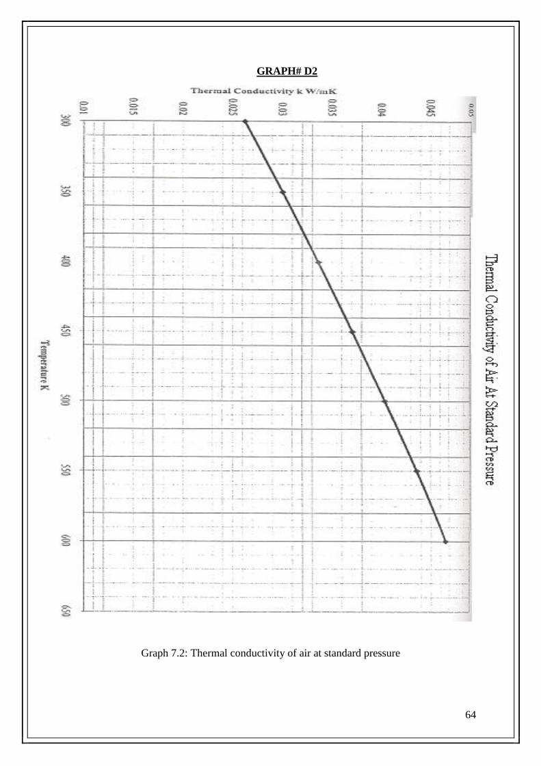
64
GRAPH# D2
Graph 7.2: Thermal conductivity of air at standard pressure

65
GRAPH# D3
Graph 7.3: Prandtl number of air at standard pressure

66
8. LAB SESSION 8
To experimentally verify the heat transfer from an extended surface from combined modes of
free conduction, free convection and radiation heat transfer by comparing it with the
theoretical analysis
8.1 Learning Objective
To analyse the increase in heat transfer by using extended surface body
8.2 Apparatus
Extended Surface Heat Transfer unit H111E (Serial no H111E/00832)
8.3 Main Parts
1) Heated cylinder
2) Eight temperature sensors (Thermocouples)
3) Heater
4) Heat transfer service unit (H111)
8.4 Useful Data
1) HEATED ROD Diameter D = 0.01m
2) Heated rod length L = 0.35m
3) Heated rod effective cross-sectional area As = 7.854 × 10⁻⁵m2
4) Heated rod surface area A = 0.01099m2
5) Thermal conductivity of heated rod material k = 121 Wm2⁄
6) Stefan Boltzmann constant σ = 5.67 × 10⁻⁸W/m2
8.5 Theory:
8.5.1 Fin (extended surface)
In the study of heat transfer, fins are surfaces that extend from an object to increase the rate
of heat transfer to or from the environment by increasing convection. The amount of
conduction, convection, or radiation of an object determines the amount of heat it transfers.
Increasing the temperature gradient between the object and the environment, increasing the
convection heat transfer coefficient, or increasing the surface area of the object increases the
heat transfer. Sometimes it is not feasible or economical to change the first two options. Thus,
adding a fin to an object, increases the surface area and can sometimes be an economical
solution to heat transfer problems.
The heat Transferred can be calculated at a given point x
𝑸𝒙 = 𝒌𝑨𝒎(𝑻𝒙 − 𝑻𝒂) 𝒕𝒂𝒏𝒉(𝒎𝑳) Equation 8.1: Heat transferred through extended
surface
While
Qx=Heat transferred at a given point x
Tx=Temperature at a given point x

67
Ta= Ambient temperature
L= Length of rod
m = √hP
kA
h=Overall heat transfer coefficient
P= Perimeter
K= Thermal conductivity
A= Heated rod surface area
8.6 Procedure:
1. Turn the voltage controller anti-clock wise to set the AC voltage to minimum. Ensure the
Extended Surface Heat Transfer Unit H111E accessory has been connected to the Heat
Transfer Service Unit H111.
2. After adjusting the heater voltage ensure that T1 (the thermocouple closest to the heater)
varies in accordance with the sense of adjustment. i.e. if the voltage is increased the
temperature T1 should also increase, if the voltage is reduced the temperature T1 should
be reduce.
3. It is now necessary that to monitor the temperature T1 to T8 until all the temperatures are
stable.
4. When T1 through T8 have reached a steady state, temperatures record the following. T1
to T9, V and I.
5. If time permits increase the voltage to a 120volts reading, repeat the monitoring of all
temperatures and when stable repeat the above readings.
6. When the experimental procedure is completed, it is good practice to turn off the power to
the heater by reducing the AC voltage to zero and leaving the fan running for a short
period until the heated cylinder has cooled. Then turn off the main switch.

68
Figure 8.1: Schematic Diagram of Experiment
8.7 Observations
Sample No 1 Distance From T1(m)
V volts - -
I Amps - -
t1 ℃ 0
t2 ℃ 0.05
t3 ℃ 0.1
t4 ℃ 0.15
t5 ℃ 0.2
t6 ℃ 0.25
t7 ℃ 0.3
t8 ℃ 0.35
t9 ℃ -
Table 8.1: Temperatures measured at different distances from T1

69
8.8 Calculated Data
Heat input Qin W
Distance x form T1 (m)
Tx − Ta
T1 − Ta
cos h[m(L − x)]
cos h [m L]
Calculated
heat
transferred
0
0.05
0.1
0.15
0.2
0.25
0.3
0.35
Table 8.2: Heat transfer from extended surface
8.8.1 Specimen Calculation
For the first sample the calculations are as follows
Qinput = V ∗ I (W)
The value of h will be that due to both convective and radiation heat transfer
h = hr + hc
For the radiant component;
hr = εFσTmean4−Ta4
Tmean−Ta =
W
m2k
Tmean = (t1+t2+t3+t4+t5+t6+t7+t8)
8+ 273.15
Ta = T9 + 273.15 (K)
Where σ = Stefan Boltzmann Constant σ = 5.67 × 10⁻⁸ W
m2 K
F = Shape factor or view factor (relating to the element geometry and the surroundings)
ε = Emissivity of the rod surface = 0.95
Ta = Absolute ambient temperature t9 + 273.15K
Tmean = Absolute mean of the measured surface temperature of the rod.
Tmean = (t1+t2+t3+t4+t5+t6+t7+t8)
8+ 273.15
For the convective component;
hc = 1.32 [Tmean − Ta
D]
0.25
= (W
m2k)

70
This is a simplified empirical equation for natural convection from a horizontal cylinder.
Where
Ta = Absolute ambient temperature t9 + 273.15K
Tmean= Absolute mean of the measured surface temperature of the rod.
D = Diameter of the rod
Hence the overall estimated heat transfer coefficient
h = hr + hc = (W
m2 K)
Now m can be determined to a reasonable degree of accuracy such that
m = √hP
kA
Where P is the perimeter of the rod = π D
Now the heat Transferred can be calculated at a given point x;
Qx = kAm(Tx − Ta) tanh(mL)
While Tan h (mL) =𝒆𝒎𝑳 −𝒆−𝒎𝑳
𝒆𝒎𝑳+𝒆−𝒎𝑳
And Cos h (mL)= 𝒆𝒎𝑳 +𝒆−𝒎𝑳
𝟐
Note: For insulated fin tip and negligible heat loss from fin tip cos h [ m(L−x)]
cos h [m L] Should be equal to
Tx−Ta
T1−Ta
8.8.2 Graph
Draw the graph b/w the distance from T1 thermocouple (X-Axis) and Temperature (Y-Axis).
8.8.3 Conclusion
8.9 Questions
1) How heat transfer is varied by varying heat transfer area
2) What is effect of perimeter on heat transfer
3) At which position, the temperature reaches the maximum value, give reason.
8.10 Comments
71
9. LAB SESSION 9
To Reduce radiation errors in measurement of temperature by using shield between sensor
and source of radiation
9.1 Learning Objective
1) To reduce the errors in temperature measurement due to radiation from a source by
using radiation shield between the sensor and the source of radiation.
9.2 Apparatus
Radiation Errors in temperature Measurements H111F (Serial no H111F/00315)
9.3 Main Parts
1) Radiant Source
2) Temperature Sensors
3) Shields of different grades
4) Main digital Control panel (H111)
9.4 Theory
The objective for the temperature sensors is to accurately measure the temperature of the air
stream. In order to do this the sensors must stabilize at the same temperatures as the air
stream. Under ideal conditions the sensors will gain or lose heat until stabilization occurs and
the sensors are at the same temperature as the air. However, if a source of thermal radiation is
visible to the sensor then depending upon the emissivity of the sensor and the source more or
less energy may be absorbed by the sensor. Hence the sensor may stabilize at a temperature
above or below the temperature of the air depending upon the temperature of the radiant
source.
The magnitude of the difference in sensor temperature relative to the air stream will depended
upon several factors.
➢ The difference in temperature between the sensor and the radiating surface.
➢ The velocity of the air passing the sensor.
➢ The size of the sensor.
➢ The emissivity of the sensor, the surroundings and the radiant source.
➢ The thermal conductivity of the sensor material and its connecting lead.
➢ Other material that may be in the air stream such as dust or water vapor.
If a suitable shield can be placed between the radiant source and the thermocouple the errors
in measurement can be reduced. Though the shield will be heated or cooled by the radiant

72
source the temperature reached by the shield will have less influence on the thermocouple
then that of the radiant source. In the apparatus, the shield is a polished stainless steel plate
that can be lowered between the ceramic heater and the three test thermocouples. The shield
allows air to pass through but prevents direct line of sight influence from the radiant source
9.5 Procedure:
1. Turn the voltage controller anti-clock wise to set the AC voltage to minimum. Ensure the
Radiation Errors H111F accessory has been connected to the Heat Transfer Service Unit
H111.
2. Ensure that the radiation shield is not fitted.
3. Turn on the main switch and the digital displays should illuminate. Select the temperature
position T10 using the rotator switch and monitor the temperatures regularly.
4. Set the temperature selector switch to display temperatures T6, T7, T8, T9 and T10 and
record the values.
5. Open the throttle butterfly but do not turn on the centrifugal fan at this point.
6. Rotate the voltage controller clockwise to increase the heater voltage to 80 Volts. Select
the T10 position on the temperature selector switch and monitor the T10 temperature.
Also monitor temperatures T7 to T9 until these reach a stable temperature (Note that the
temperatures may not be equal).
7. When the temperatures are stable record T6, T7, T8, T9, T10, V, and I.
8. Rotate the voltage controller clockwise to increase the heater voltage to 120 Volts. Again
allow the temperatures to stabilize and then record T6, T7, T8, T9, T10, V, and I.
9. Repeat the above procedure at heater voltages of 180 and 230 volts (Note that the heater
temperature T10 should not be allowed to exceed 400℃).
10. Completely close the throttle butterfly on the fan intake and then turn on the centrifugal
fan.
11. Adjust the throttle until a velocity of approximately 0.5m/s is indicated.
12. Observe the temperature T6 to T10 and when stable record T6, T7, T8, T9, T10, V, and I.
13. Increase the air velocity to 1m/s, allow the temperatures to stabilize and repeat the
observations. Further increase the velocity to 2m/s and 4m/s and again repeat the
observations.
14. Repeat all the procedure for objective 2 by using the radiation shield.
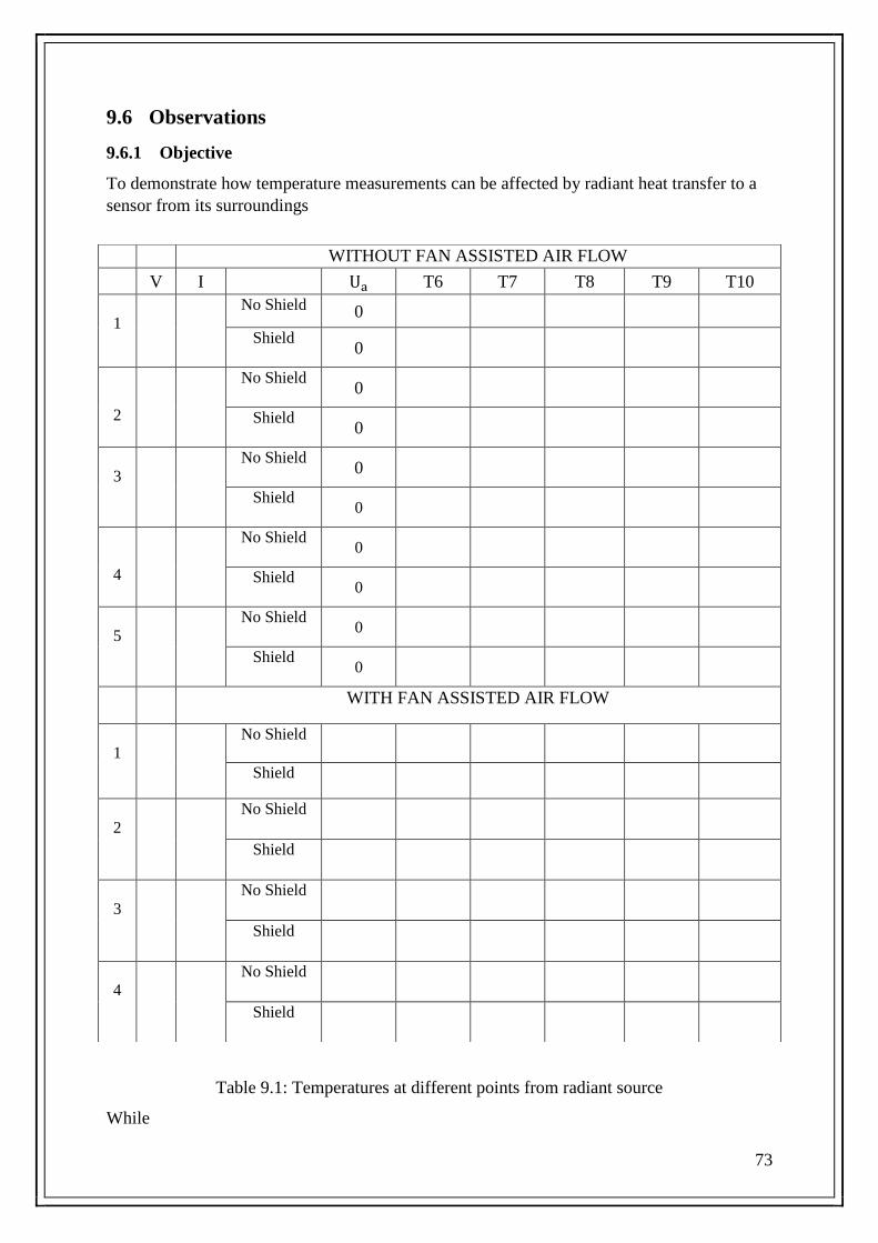
73
9.6 Observations
9.6.1 Objective
To demonstrate how temperature measurements can be affected by radiant heat transfer to a
sensor from its surroundings
Table 9.1: Temperatures at different points from radiant source
While
WITHOUT FAN ASSISTED AIR FLOW
V I Ua T6 T7 T8 T9 T10
1
No Shield 0
Shield 0
2
No Shield 0
Shield 0
3
No Shield 0
Shield 0
4
No Shield 0
Shield 0
5
No Shield 0
Shield 0
WITH FAN ASSISTED AIR FLOW
1
No Shield
Shield
2
No Shield
Shield
3
No Shield
Shield
4
No Shield
Shield

74
V= Voltage
I= Current, T6= Temperature of air and T7, T8, T9= Temperature at different points
T10= Temperature of heater
Ua= Air velocity
9.6.1.1 Graph
i) Draw the graph b/w heater volts (V) along x-Axis and Temperature T6, T7, T8,
T9 along Y-Axis. (i.e. V vs T6, V vs T7, V vs T8, V vs T9, V vs T10) with shield
and without shield
9.6.1.2 Conclusion
9.7 Comments

75
10. LAB SESSION 10
To determine the Convective heat transfer coefficient of a solid cylinder using analytical
transient temperature/heat flow charts
10.1 Learning Objective
1) Use of heisler charts for lumped heat capacity system
2) Use of properties like biot number and fourier number to calculate convective heat
transfer unit
10.2 Apparatus
Heat Transfer service unit with Unsteady State Heat Transfer Unit H111G
10.3 Main Parts
1) Drain Valve
2) Water supply
3) Pump
4) 20mm diameter Brass cylinder
5) Temperature sensors prob
6) water bath
7) 20 mm diameter stainless steel cylinder
10.4 Theory
10.4.1 Transient Heat-Transfer
If a solid body is suddenly subjected to a change in environment, some time must elapse
before an equilibrium temperature condition will prevail in the body. In the transient heating
or cooling process that takes place in the interim period before equilibrium is established, the
analysis must be modified to take into account the change in internal energy of the body with
time, and the boundary conditions must be adjusted to match the physical situation that is
apparent in the unsteady-state heat-transfer problem. Unsteady-state heat-transfer analysis is
obviously of significant practical interest because of the large number of heating and cooling
processes that must be calculated in industrial applications
10.4.2 Lumped-Heat-Capacity System
Transient heat conduction can be analyzed in systems that may be considered uniform in
temperature. This type of analysis is called the lumped-heat-capacity method. Such systems
are obviously idealized because a temperature gradient must exist in a material if heat is to be
conducted into or out of the material. In general, the smaller the physical size of the body, the
more realistic the assumption of a uniform temperature throughout; in the limit a differential
volume could be employed as in the derivation of the general heat-conduction equation
10.4.3 Biot number (Bi)
The Biot number (Bi) is a dimensionless quantity used in heat transfer calculations. It is
named after the French physicist Jean-Baptiste Biot (1774–1862), and gives a simple index of
the ratio of the heat transfer resistances inside of and at the surface of a body. This ratio

76
determines whether or not the temperatures inside a body will vary significantly in space,
while the body heats or cools over time, from a thermal gradient applied to its surface. In
general, problems involving small Biot numbers (much smaller than 1) are thermally simple,
due to uniform temperature fields inside the body. Biot numbers much larger than 1 signal
more difficult problems due to non-uniformity of temperature fields within the object. It
should not be confused with Nusselt number, which employs the thermal conductivity of the
fluid and hence is a comparative measure of conduction and convection, both in the fluid.The
Biot number has a variety of applications, including transient heat transfer and use in
extended surface heat transfer calculations.
The Biot number is defined as
Bi=𝒉𝑳
𝒌 Equation 10.1: Biot number
h = film coefficient or heat transfer coefficient or convective heat transfer coefficient
L = characteristic length, which is commonly defined as the volume of the body
divided by the surface area of the body, such that L=Volume
Area
k = Thermal conductivity of the body
The physical significance of Biot number can be understood by imagining the heat flow from
a small hot metal sphere suddenly immersed in a pool, to the surrounding fluid. The heat flow
experiences two resistances: the first within the solid metal (which is influenced by both the
size and composition of the sphere), and the second at the surface of the sphere. If the thermal
resistance of the fluid/sphere interface exceeds that thermal resistance offered by the interior
of the metal sphere, the Biot number will be less than one. For systems where it is much less
than one, the interior of the sphere may be presumed always to have the same temperature,
although this temperature may be changing, as heat passes into the sphere from the surface.
The equation to describe this change in (relatively uniform) temperature inside the object is
simple exponential one described in Newton's law of cooling.
In contrast, the metal sphere may be large, causing the characteristic length to increase to the
point that the Biot number is larger than one. Now, thermal gradients within the sphere
become important, even though the sphere material is a good conductor. Equivalently, if the
sphere is made of a thermally insulating (poorly conductive) material, such as wood, the
interior resistance to heat flow will exceed that of the fluid/sphere boundary, even with a
much smaller sphere. In this case, again, the Biot number will be greater than one.
10.4.4 Fourier number (Fo)
Fourier number (Fo) or Fourier modulus, named after Joseph Fourier, is a dimensionless
number that characterizes transient heat conduction. Conceptually, it is the ratio of diffusive
or conductive transport rate to the quantity storage rate, where the quantity may be either heat
(thermal energy) or matter (particles). The number derives from non-dimensionalization of
the heat equation (also known as Fourier's Law) or Fick's second law and is used along with
the Biot number to analyze time dependent transport phenomena.
The general Fourier number is defined as

77
Fo=Diffusive transport rate
Storage rate
Fo = 𝛼 X t
(Length)2 Equation 10.2: Fourier
number
α =k
ρc Equation 10.3:
Thermal diffusivity
α is the thermal diffusivity (SI units: m2/s)
t is the characteristic time (s)
L is the length through which conduction occurs (m)
K is thermal conductivity (W/(m·K))
ρ is density (kg/m³)
c is specific heat capacity (J/(kg·K))
10.4.5 Heisler charts
Heisler charts are a graphical analysis tool for the evaluation of heat transfer in thermal
engineering. They are a set of two charts per included geometry introduced in 1947 by M. P.
Heisler. which were supplemented by a third chart per geometry in 1961 by H. Gröber.
Heisler charts permit evaluation of the central temperature for transient heat conduction
through an infinitely long plane wall of thickness 2L, an infinitely long cylinder of radius ro,
and a sphere of radius ro.
Although Heisler-Gröber charts are a faster and simpler alternative to the exact solutions of
these problems, there are some limitations. First, the body must be at uniform temperature
initially. Additionally, the temperature of the surroundings and the convective heat transfer
coefficient must remain constant and uniform. Also, there must be no heat generation from
the body itself.
10.5 Procedure
1. Ensure that the residual current circuit breaker (RCCB) is open-circuit. Ensure that
the drain valve adjacent to the circulating pump is in the closed position and half-fill
the water bath with clean water.
2. Pump bleeding- Switch on the RCCB/MCB to cause the pump to run. Incline the
pump by lifting the baseboard from the front to allow the air to escape. Noise from the
pump is the sign of trapped air. A bleed screw is fitted to the head of the pump.
3. Continue the filling of bath until the water level is at mid height of the holes in the
flow duct. If the local water contains of a large amount of dissolved solids that
normally result in scale build up then it is recommended that the bath id fitted with

78
de-ionized or mineralized water. Ensue that the thermostat has been turned fully anti-
clockwise and is in the off position.
4. Ensure that the H111 unit main switch is in the off position (None of three digital
displays should be illustrated). Ensure that the residual current circuit breaker on the
H111 rear panel is in the ON position. Ensure that the residual current circuit breaker
on the H111G baseboard is in the on position. Not that the residual current circuit
breaker on the both units (H111 and H111G) should be tested for normal operation at
intervals specified by local regulations.
5. Turn on the power supply to the Unsteady State Heat Transfer unit and turn on the
16A Heater miniature circuit breaker (MCB). Ensure that the red power indicator
adjacent to the thermostat is illustrated. Turn the thermostat to position 6 for faster
heating. The water will take approximately 30 minutes to heat from cold. At this
setting the water will boil, if left unattended. While the water bath is heating the
following may be auctioned.
6. Install the 20mm diameter brass cylinder in the shape carrier.
7. Insert the T3 probe to engage fully into the center of the shape.
8. Insert the T2 probe to sense water temperature adjacent to the shape.
9. Avoid touching the shape by hand to reduce thermal effects and place the shape on
the bench to reach ambient temperature.
10. The water bath temperature T1 should be stabilized at approximately 80 to 90˚C
11. Set the circulating pump to 3 and therefore the water flow velocity in the flow duct.
12. Turn on the power supply to the Heat Transfer Service Unit H111 and main switch
and three digital displays illustrate. Set the temperature selector switch to the T1to
indicate the temperature of the bath. Observe the T1 to confirm that it is slowly
increasing as the bath is heated.
13. Record the start conditions temperatures and then plunge the shapes in the flow duct.
Then record temperatures and time.
14. Observe the T1. If the bath temperature exceeds that is required, reduce the thermostat
setting to OFF and wait for the water to cool. The water bath temperature T1 should
not be allowed to exceed 85-90 as the pump will cavitate.
15. Once the 20mm diameter brass has reached the water bath temperature, remove it
from the tank install the 20mm stainless steel cylinder in the shape carrier.
16. Record the starting condition temperatures and then plunge the shape in the flow duct.
Then record temperatures and time.
17. Having achieved the desired temperature, say85, reduces the thermometer setting to
position 2. It will cycle ON/OFF to maintain the existing temperature.
18. If time permits the procedures may be repeated for the brass and stainless-steel sphere
and/or the Brass and Stainless Slab.
19. In addition, by varying the circulating pump speed, the effect of variation of water
velocity on local heat transfer coefficient may be investigated.

79
20. When the experimental procedure is completed, it is good habit to turn off the power
to the heater by reducing the AC voltage to zero. And fan leaving the fan running for
a short period until the heater has cooled. Then turn off the main switch.
10.6 Observations
Recorded Time T1
Bath Temp.
T2
Air/ Water Temp.
T3
Geometric Centre Temp.
Seconds ºC ºC ºC
0
5
10
15
20
25
30
35
40
Table 10.1: Specimen: 20mm diameter Brass Cylinder.
Recorded Time T1
Bath Temp.
T2
Air/ Water Temp.
T3
Geometric Centre Temp.
Seconds ºC ºC ºC
0
5
10
15
20
25
30
35
40
Table 10.2: Specimen: 20mm Stainless Steel Cylinder

80
10.7 Calculated Data
Recorded
Time
T1
Bath
Temperature
T3
Geometric
Centre
Temperature
θ
Non-
dimensional
Temperature
Fo
Fourier
Number
1/Bi
Inverse Biot
Number
(h)
Convective
heat
transfer
coefficient
Seconds
0
5
10
15
20
25
30
35
40
Table 10.3: Properties of Specimen: 20mm diameter Brass Cylinder
Recorded
Time
T1
Bath
Temperature
T3
Geometric
Centre
Temperature
θ
Non-
dimensional
Temperature
Fo
Fourier
Number
1/Bi
Inverse Biot
Number
(h)
Convective
heat
transfer
coefficient
Seconds
0
5
10
15
20
25
30
35
40
Table 10.4: Properties of Specimen: 20mm diameter stainless steel Cylinder
10.7.1 Sample Calculations
The calculation procedure for system with finite internal and surface heat transfer resistance
is as follows.
For each sample after intermission the non-dimensional temperature 𝜃 is calculated.
Tc = T3
T∞ = T1
Ti = T3 at time 0
θ =Tc− T∞
Ti− T∞=
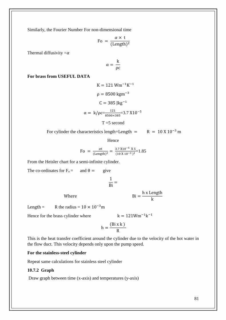
81
Similarly, the Fourier Number For non-dimensional time
Fo = 𝛼 × t
(Length)2
Thermal diffusivity =𝛼
α = k
ρc
For brass from USEFUL DATA
K = 121 Wm−1K−1
ρ = 8500 kgm−3
C = 385 Jkg−1
α = k/ρc=121
8500×385=3.7 X10⁻⁵
T =5 second
For cylinder the characteristics length=Length = R = 10 X 10−3 m
Hence
Fo = 𝛼t
(Length)2 = 3.7 X10−5 X 5
(10 X 10−3 )2 =1.85
From the Heisler chart for a semi-infinite cylinder.
The co-ordinates for Fo = and θ = give
1
Bi=
Where Bi =h x Length
k
Length = R the radius = 10 × 10−3m
Hence for the brass cylinder where k = 121Wm−1k−1
h =(Bi x k )
R
This is the heat transfer coefficient around the cylinder due to the velocity of the hot water in
the flow duct. This velocity depends only upon the pump speed.
For the stainless-steel cylinder
Repeat same calculations for stainless steel cylinder
10.7.2 Graph
Draw graph between time (x-axis) and temperatures (y-axis)

82
10.7.3 Conclusion
10.8 Statistical Analysis
NIL
10.9 Questions
1) How the temperature is distributed at different interval of time
2) What is Fourier Number
3) What is Biot number
4) What is Transient Heat-Transfer
5) What is Lumped-Heat-Capacity System
6) How Geometric Centre Temp is distributed at different intervals of time
7) How Fourier number and Biot number vary with time. Give reason
10.10 Comments
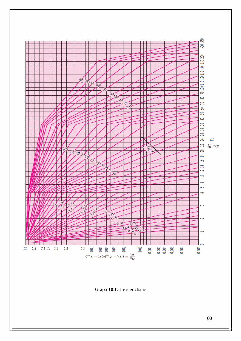
83
Graph 10.1: Heisler charts

84
11. LAB SESSION 11
To measure the effect of different exchanger geometry on convection heat transfer
mechanism
11.1 Learning Objective
1) Measure temperatures of different points in Free and forced convection in flat surfaces
2) Measure the dependence of the heat transmission on exchanger geometry.
11.2 Apparatus
Free and forced convection heat transfer unit TCLFC (Serial No= TCLFC 0009/07)
11.3 Main Parts
1) Stainless steel tunnel of rectangular section
2) Flat exchanger, tenon exchanger and fins exchanger
3) Thermocouple
4) fan supply
5) A branded computer attached to unit
6) Interface
11.4 Useful Data
• Structure of anodized aluminium that guarantees a good stability and resistance to the
environment.
• Stainless steel tunnel 700 mm long, painted and resistant to corrosion.
• Methacrylate viewer that allows a good visualization of the exchanger that is in use.
• Grey PVC stabilizers to guarantee a uniform air flux.
• Thermocouples type J.
• Maximum working temperature: 100ºC.
• Flow sensor with digital output.
• Aluminium exchangers of flat, spiked and bladed surfaces.
• Heating resistances of 150W.
Dimensions and weights
• Approximate dimensions of the equipment: 37x61x92
• Approx. shipment volume: 0.2m3
• Approx. weight: 10 Kg

85
11.5 Theory
Convection is the term used for the process of energy transmission, which takes place in the
fluid mainly due to the energy transported by the movement of the fluid. The conduction
energy process by molecular exchange is, as logical, always present. However, big quantities
of energy (or heat) of the fluids are in contact with regions of inferior energy (colder regions)
due to the existence of big displacements of the fluid particles. If external forces in form of
difference of pressures produce the movement of the fluid, this mechanism is called forced
convection. An example of forced convection is the pumping of a fluid, in contact with solid
surfaces at different temperatures to that of the fluid. If no external forces are applied to a
fluid, it can move due to density differences that could be produced by a solid body
submerged in a fluid whose temperature is different to that of the fluid. This type of heat
exchange is called free
Convection and it can be observed in a recipient with boiling water, in the air that surrounds
radiators in rooms, etc. The following theoretical analysis uses an empirical relationship for
the heat transfer due to natural convection proposed by WH McAdams in the publication
"Heat Transmission", third edition, McGraw-Hill, New York, 1959
Heat loss due to natural convection: Qc = hc As (Ts - Ta)
Equation 8.1
Heat transfer area (surface area): As = (π D L)
Equation 8.2
The heat transfer coefficient hc can be calculated using the following relationships
hc=1.32 [Ts−Ta
D]
0.25
Equation 8.3
Ts = Surface temperature of cylinder (K)
Ta = Ambient temperature (K)
11.5.1 Introduction of The Equipment
Figure 8.1: Schematic Diagram of Experiment
Simultaneous heat transference by conduction and convection (free or forced) is the base of
several industrial heat exchangers, as well as the several devices related to them. This
86
equipment of EDIBON allows studying the efficiency of different exchangers, analyzing the
heat transmission coefficients of each of the exchangers exposed to different airflows. A fan
placed in the upper part of the tunnel allows
controlling the airflow that goes through the tunnel. An interface connectable to a PC
contains the control circuits to measure temperatures, electrical control, electrical supply and
speed control of the fan.
The interface provides an output to a PC where the values and graphics of all the variables
involved in the practices are shown. The airflow is measured with a flowmeter set on the
inferior part of the tunnel. This EDIBON equipment allows making a study of the heat
transmission in three different types of exchangers
1. Flat exchanger
2. Tenon exchanger
3. Fins exchanger
11.5.2 Description of The Equipment
The equipment consists of a stainless-steel tunnel of rectangular section supported by a
structure in anodized aluminium that allows to be set on the worktable. In the tunnel, three
types of different heat exchangers can be set: flat exchanger, tenon exchanger and fins
exchanger. Each exchanger has an electric
resistance for its heating. In the three bases of the exchangers we set a thermocouple that
serves to control the temperature that the exchangers reach. The heat exchanger that is used in
each moment can be observed by a methacrylate window placed in the opposite side of the
tunnel The rising air flux through the tunnel can be generated by a variable speed fan set on
the superior part. The airflow generated in the tunnel is measured by a flow meter placed in
the inferior part of the tunnel. By some air flux concentrators a correct distribution of the
airflow is guaranteed by the area of heat exchange. Two thermocouples measure the air
temperature at the inlet and outlet of the area of heat exchange. Temperature measurements,
at different distances of the base of the tenon and fins exchangers, are made by other five
thermocouples that are introduced by one side of the tunnel. These measurements allow
observing the gradients of temperature
in the longitudinal direction of the exchangers and in the direction of the air flux. An
interface receives the signal of all the thermocouples and the flow meter, providing a
computerized outlet of all the measurements. By the interface we make a control of
temperature at the bases of the exchangers. Besides, the fan supply and the electrical
resistance are provided by the interface. The electric supply of all the equipment is made by
the connection of the interface to the net.
11.6 Objective: 1
To demonstrate the relationship between power input and surface temperature in free
convection
11.6.1 Procedure
1. We will start taking the measure of the surface that exchanges heat.
2. Next, we place the flat exchanger in the tower
3. We insert the thermocouples. A thermocouple will be placed in the exchanger, and the
other three in the three orifices placed in the middle of the tunnel.

87
4. The equipment is connected. The power of the resistance is regulated in fixed values.
5. When the temperatures are established we will proceed to its measurement, as well as
that of the air speed.
6. Once all the measures are taken the equipment is unplugged. When some time has
gone by, the thermocouples and the exchanger are removed
7. Repeat the experiment by turning the fan in “ON” position
11.6.2 Observations
Table 11.1: Temperatures in free convection
Table 11.2: Temperatures in forced convection
11.6.3 Graph
Draw the Graph of temperatures (y-Axis) and AR-1 (X- Axis) for free as well as in forced
convection
11.6.4 Conclusion
No AR-1
(Ohm)
SC-1
(l/s)
ST-1
(°C)
ST-2
(°C)
ST-3
(°C)
ST-4
(°C)
ST-5
(°C)
ST-6
(°C)
ST-7
(°C)
No AR-1
(Ohm)
SC-1
(l/s)
ST-1
(°C)
ST-2
(°C)
ST-3
(°C)
ST-4
(°C)
ST-5
(°C)
ST-6
(°C)
ST-7
(°C)

88
11.7 Objective: 2
Measure dependence of the heat transmission on exchanger geometry
11.7.1 Procedure
1. You will begin placing the blade exchanger in the tower. Next, the thermocouples are
introduced to measure the temperature in the base of the exchanger, that of the inlet
air and that of outlet.
2. Fix the electric power of the resistance and the speed of the fan at fixed values
3. Once the measures are taken, repeat the experiment with the spike exchanger.
11.7.2 Observations:
Table 11.3: Temperatures for different geometry of exchangers
11.7.3 Graph
Draw the Graph of temperatures (y-Axis) and AR-1 (X- Axis)
11.7.4 Conclusion
11.8 Specimen Calculation
NIL
No AR-1
(Ohm)
SC-1
(l/s)
ST-1
(°C)
ST-2
(°C)
ST-3
(°C)
ST-4
(°C)
ST-5
(°C)
ST-6
(°C)
ST-7
(°C)
Blade
Heat
exchanger
spike
exchanger

89
11.9 Statistical Analysis
NIL
11.10 Questions
1) Write is difference on temperatures in free and forced convection. Explain
2) What is free and forced convection
3) What is effect on heat transfer by changing the geometry of exchanger
11.11 Comments

90
12. LAB SESSION 12
To calculate logarithmic mean temperature difference (LMTD), global heat transfer
coefficient and effectiveness of turbulent flow heat exchanger
12.1 Learning Objective
1) Balance the energy in the Turbulent Flow exchanger.
2) Calculate the heat exchanger effectiveness by NTU method.
12.2 Apparatus
Turbulent Flow Heat Exchanger (TIFTC) (Serial no TIFT 0003/06)
12.3 Main Parts
IDENTIFICATION DESCRIPTION
ST-1 Temperature sensor in the water tank.
ST-2 Cold water temperature sensor at the exchanger inlet or outlet
ST-3 Hot water sensor at the exchanger inlet
ST-4 Cold water sensor between the first and second stretch of the
exchanger
ST-5 Hot water sensor between the first and second stretch of the
exchanger
ST-6 Cold water sensor between the second and third stretch of the
exchanger
ST-7 Hot water sensor between the second and third stretch of the
exchanger
ST-8 Cold water temperature sensor at the exchanger inlet or outlet
ST-9 Hot water sensor at the exchanger outlet
ST-10 Temperature sensor of the exterior surface of the interior tube at the
exchanger
Inlet.
ST-11 Temperature sensor of the exterior surface of the interior tube at the
exchanger
Outlet
SC-1 Hot water flow sensor
SC-2 Cold water flow sensor
AVR-1 Hot water flow regulation valve.
AVR-2 Cold water flow regulation valve
AN-1 Water level switch of the tank
AR-1 Electric resistance
AB-1 Centrifugal pump for hot water circulation
AP-1 Cold water circuit purge
AP-2 Hot water circuit purge
AV-2,AV-3, AV-4
and AV-5
Ball valves of the cold water circuit to fix parallel or crosscurrent
flow
AV-1,AV-6, AV-7
and AV-8
Ball valves to drain the pipes

91
12.4 Useful Data
Exchange Length: L = 3 × 0.5 = 1.5 m.
12.4.1 Interior Tube
Internal Diameter: Dint = 8×10- 3 m
External Diameter: Dext = 10×10- 3 m
Thickness = 10- 3 m
Internal heat transference area: Ah = 0.0377 m2
External heat transference area: Ac = 0.0471 m2
12.4.2 Exterior Tube
Internal Diameter: Dint,c =13×10- 3 m
External Diameter: Dext,c =15×10- 3 m
Thickness = 10- 3 m
12.4.3 Base Unit
Net weight: 30 kg.
Height: 400 mm
Width: 1000 mm
Depth: 500 mm
12.4.4 Heat Exchanger
Net weight: 20 kg.
Height: 200 mm
Width: 1000 mm
Depth: 500 mm
12.4.5 Physical Properties of The Hot And Cold Water
To determine their physical properties, the average temperature of each fluid has to be
calculated.
Hot water average temperature: Tmh = ST3+ST9
2
Cold Water Average Temperature: Tmc =ST2+ST8
2
From the table of the appendix A, the physical properties based on the average temperature
can be obtained
12.4.6 Mass Flow Rates
The mass flows of both fluids, are going to be obtained from the measurements taken in
the flow sensors (SC1 for hot water and SC2 for cold water)
𝜌 Cp=Specific
heat(J/kgK) 𝜇= Dynamic viscosity
(kg/ms)
Hot water at Tmh °C 𝜌h= Cph 𝜇h
Cold water at Tmc °C 𝜌c= Cph 𝜇c

92
m (kg/s) = 𝜌.SC= ρ (
kg
m3).SC(l
min)
60×1000
Mass flow for hot water= mh (kg/s) = 𝜌.SC= ρh (
kg
m3).SC(litre
min)
60×1000=……..kg/s
Mass flow for cold water= mc (kg/s) = 𝜌.SC= ρc (
kg
m3).SC(litre
min)
60×1000=……..kg/s
Figure 12.1: Schematic Diagram of Experiment
12.5 Theory
12.5.1 Heat transference in heat exchangers
A heat exchanger is a device developed by humans for the heat transference between two
fluids at different temperatures separated by a solid wall. They have many engineering
applications and, as a consequence, there are many models adapted to each application. The
simplest one is the one built with two concentric tubes, where fluids can move in the same
sense or in the opposite one. In parallel flow, the hot and the cold water go in and out through
the same end. In crosscurrent flow, the fluids go in and out through opposite ends and they
circulate in opposite senses.

93
12.5.2 Overall Heat-Transfer Coefficient
The overall heat-transfer coefficient U is defined by the relation
q=UA∆Toverall Equation 12.1 Overall heat transfer coefficient
Although final heat-exchanger designs will be made on the basis of careful calculations of U,
it is helpful to have a tabulation of values of the overall heat-transfer coefficient for various
situations that may be encountered in practice
12.5.3 The Log Mean Temperature Difference (LMTD)
Being ∆T1 = Th,i - Tc,i and ∆T2 = Th,o - Tc,o in parallel flow
And
∆T1 = Th,i - Tc,o and ∆T2 = Th,o - Tc,i in counter current flow.
Tlm=(∆T1)−(∆T2)
ln [∆T1
∆T2]
Equation 12.2: The Log Mean Temperature Difference
12.5.4 Effectiveness-Ntu Method
Effectiveness= Actual heat transfer
Maximum possible heat transfer Equation 12.3
12.5.5 Capacity coefficient
Capacity coefficient will be defined as (CR)
Cr=Cmin
Cmax=……….
w/k
w/k Equation 12.4
Mass flow rate multiplied by specific heat) Ch and Cc for the hot and cold fluids respectively,
and denoting the smaller one as Cmin

94
12.5.6 Reynolds number
Reynolds number (Re) is a dimensionless quantity that is used to help predict similar flow
patterns in different fluid flow situations. The Reynolds number is defined as the ratio of
momentum forces to viscous forces and consequently quantifies the relative importance of
these two types of forces for given flow conditions. They are also used to characterize
different flow regimes within a similar fluid, such as laminar or turbulent flow
1) Laminar flow occurs at low Reynolds numbers, where viscous forces are dominant,
and is characterized by smooth, constant fluid motion;
2) Turbulent flow occurs at high Reynolds numbers and is dominated by inertial forces,
which tend to produce chaotic eddies, vortices and other flow instabilities.
Readers can read further detail from book “heat transfer by J.P Holman” in “chapter 10”
12.6 Objective 01
Balance the energy in the Turbulent Flow exchanger.
12.6.1 Procedure:
1. Check that the valves are opened and that we have crosscurrent flow configuration.
2. Check that the heating tank is full of water, above the level switch
3. Switch on the pump and the resistor (Equipment supply)
4. Fix the tank temperature at 50 °C (STI)
5. Fix the hot water flow in 3 l/min (SCI) and adjust the cold-water flow until reaching
stationary operation conditions maintaining constant the temperature fixed in the tank.
6. Note down the temperature and flow measures in the experimental sheet
7. Repeat steps 5 and 6 for different water temperatures in the deposit 55 °C, 60°C and 65
°C.
8. Once the measures are made, Calculate the heat transferred by the hot water, the heat
absorbed by the cool water, the heat loses, the logarithmic mean temperature and global
heat transference coefficient

95
12.6.2 Observations
Table 12.1: Temperature at different points of turbulent flow heat exchanger
12.6.3 Calculated Data
Table 12.2: Heat transfer calculation in turbulent flow heat exchanger
TEST 1 TEST 2 TEST 3 TEST 4
ST1 (°C)
ST2 (°C)
ST3 (°C)
ST4 (°C)
ST5 (°C)
ST6 (°C)
ST7 (°C)
ST8 (°C)
ST9 (°C)
ST10 (°C)
ST11 (°C)
SC1 (l/min) 3 3 3 3
SC2 (l/min)
TEST 1 TEST 2 TEST 3 TEST 4
qh (w)
qc (w)
ql (w)
∆Tlm (K)
U (w/m2k)
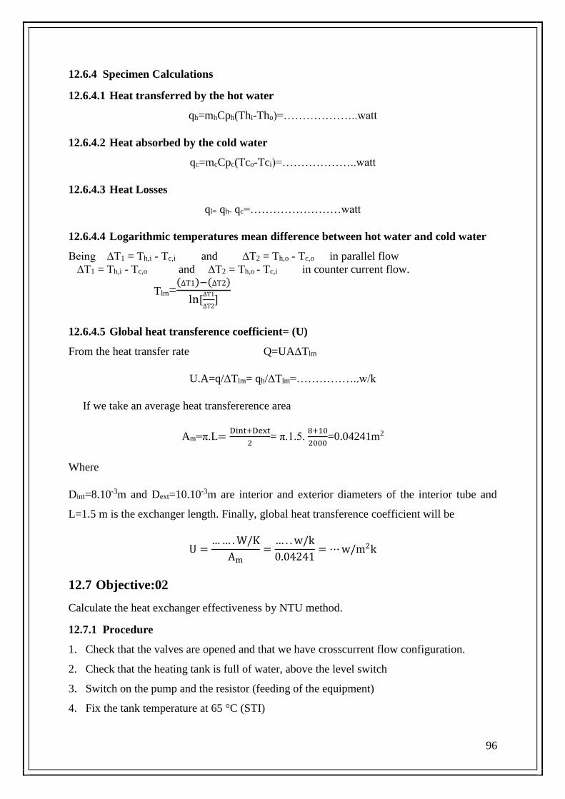
96
12.6.4 Specimen Calculations
12.6.4.1 Heat transferred by the hot water
qh=mhCph(Thi-Tho)=………………..watt
12.6.4.2 Heat absorbed by the cold water
qc=mcCpc(Tco-Tci)=………………..watt
12.6.4.3 Heat Losses
ql= qh- qc=……………………watt
12.6.4.4 Logarithmic temperatures mean difference between hot water and cold water
Being ∆T1 = Th,i - Tc,i and ∆T2 = Th,o - Tc,o in parallel flow
∆T1 = Th,i - Tc,o and ∆T2 = Th,o - Tc,i in counter current flow.
Tlm=(∆T1)−(∆T2)
ln [∆T1
∆T2]
12.6.4.5 Global heat transference coefficient= (U)
From the heat transfer rate Q=UA∆Tlm
U.A=q/∆Tlm= qh/∆Tlm=……………..w/k
If we take an average heat transfererence area
Am=π.L=Dint+Dext
2= π.1.5.
8+10
2000=0.04241m2
Where
Dint=8.10-3m and Dext=10.10-3m are interior and exterior diameters of the interior tube and
L=1.5 m is the exchanger length. Finally, global heat transference coefficient will be
U =… … . W/K
Am=
… . . w/k
0.04241= ⋯ w/m2k
12.7 Objective:02
Calculate the heat exchanger effectiveness by NTU method.
12.7.1 Procedure
1. Check that the valves are opened and that we have crosscurrent flow configuration.
2. Check that the heating tank is full of water, above the level switch
3. Switch on the pump and the resistor (feeding of the equipment)
4. Fix the tank temperature at 65 °C (STI)
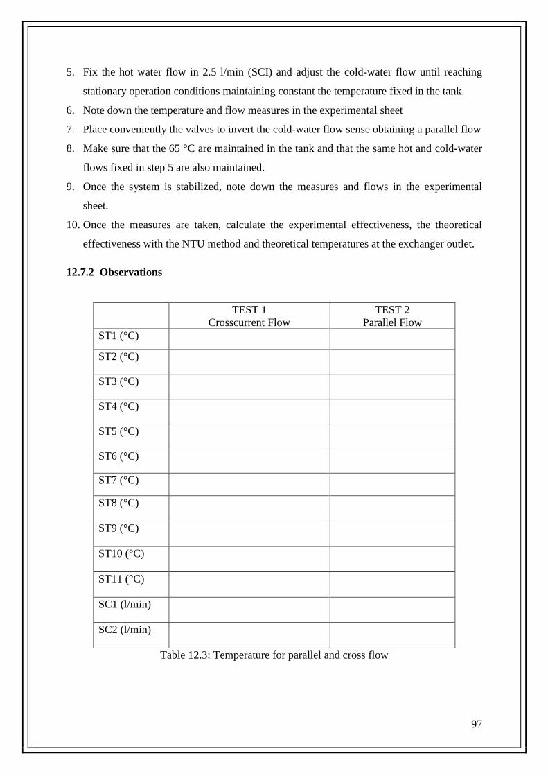
97
5. Fix the hot water flow in 2.5 l/min (SCI) and adjust the cold-water flow until reaching
stationary operation conditions maintaining constant the temperature fixed in the tank.
6. Note down the temperature and flow measures in the experimental sheet
7. Place conveniently the valves to invert the cold-water flow sense obtaining a parallel flow
8. Make sure that the 65 °C are maintained in the tank and that the same hot and cold-water
flows fixed in step 5 are also maintained.
9. Once the system is stabilized, note down the measures and flows in the experimental
sheet.
10. Once the measures are taken, calculate the experimental effectiveness, the theoretical
effectiveness with the NTU method and theoretical temperatures at the exchanger outlet.
12.7.2 Observations
Table 12.3: Temperature for parallel and cross flow
TEST 1
Crosscurrent Flow
TEST 2
Parallel Flow
ST1 (°C)
ST2 (°C)
ST3 (°C)
ST4 (°C)
ST5 (°C)
ST6 (°C)
ST7 (°C)
ST8 (°C)
ST9 (°C)
ST10 (°C)
ST11 (°C)
SC1 (l/min)
SC2 (l/min)

98
12.7.3 Calculations
From these measures, calculate the following thermodynamic variables
Experimental effectiveness (ϵ)
Heat transferred by the hot water (qh)
Logarithmic temperatures mean difference between hot and cold water (∆Tlm)
Parameters: U.A, NTU and CR
Effectiveness obtained by NTU method (ϵNTU)
Hot and cold water temperatures at the exchanger outlet obtained from the experimental
effectiveness (Th,˳y,Tc,o)
Table 12.4: Effectiveness of turbulent flow exchanger
12.7.4 Specimen Calculations
The effectiveness is the quotient between the heat really exchanged and the maximum heat
that could be transferred in an infinite area exchanger in a crosscurrent flow.
If mhCph˂mcCpc ϵ=(Th,i)−(Th,o)
Th,i−Tc,o
mhCph ˃mcCpc ϵ=(Tc,o)−(Tc,i)
Th,i−Tc,i
12.7.4.1 Heat transferred by the hot water
qh=mhCph(Thi-Tho)=………………..watt
12.7.4.2 Logarithmic temperatures mean difference between hot water and cold water
Being ∆T1 = Th,i - Tc,i and ∆T2 = Th,o - Tc,o in parallel flow
∆T1 = Th,i - Tc,o and ∆T2 = Th,o - Tc,i in counter current flow.
TEST 1
Crosscurrent Flow
TEST 2
Parallel flow
ϵ
qh (w)
∆Tlm (K)
U.A (w/k)
NTU
CR
ϵNTU

99
Tlm=(∆T1)−(∆T2)
ln [∆T1
∆T2]
From the heat transfer rate Q=UA∆Tlm
U.A=q/∆Tlm= qh/∆Tlm=……………..w/k
12.7.4.3 Number of transmission units
Calculating NTU
NTU= ϵ=U.A
(m.Cp)min
12.7.4.4 Capacity coefficient
Capacity coefficient is determined by
Cr=mCpmin
mCpmax=……….
w/k
w/k
Once the NTU and Cr are obtained, we can calculate the effectiveness, but depending if the
flow is in crosscurrent or in parallel flow, we will have to use different expressions
ϵNTU=1−e−NTU.(1+CR)
1+CR For Parallel flow
ϵNTU=1−e−NTU.(1−CR)
1−CR× e−NTU.(1−CR) For Crosscurrent flow
Comparing the value of ϵ with ϵ NTU we will have to observe if both values are similar or, if
on the other hand, they are very different one from each other
12.8 Graph
Draw the graph between the temperature distribution for parallel and crosscurrent flow. To do
this, place temperature values on the vertical (y-) axis for the hot water, cold water and of the
interior tube surface in ºC (T); and in the x-axis place the position along the exchanger in
meters (x). Take into account that the exchange length is 1.5m and that there are four points
to measure the temperature
12.9 Statistical Analysis
1) xavg= x1+x2+x3
n
2) Sx=√1
𝑛−1((𝑥1 − 𝑥𝑎𝑣𝑔)2 + (𝑥2 − 𝑥𝑎𝑣𝑔)2 + (𝑥3 − 𝑥𝑎𝑣𝑔)2)
12.10 Conclusion

100
12.11 Questions
1) What is the difference between the temperature distribution for parallel and
crosscurrent flow?
2) What is Global heat transference coefficient
3) What is Logarithmic temperatures mean difference
12.12 Comments
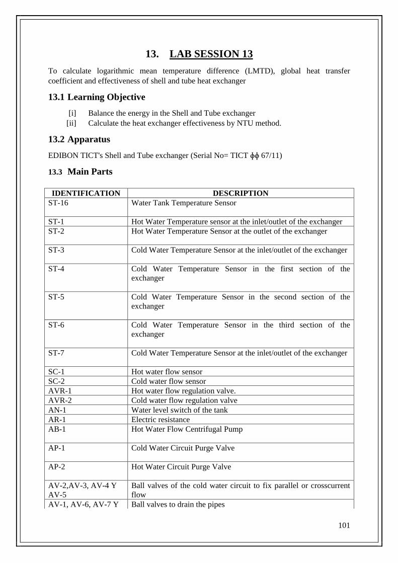
101
13. LAB SESSION 13
To calculate logarithmic mean temperature difference (LMTD), global heat transfer
coefficient and effectiveness of shell and tube heat exchanger
13.1 Learning Objective
[i] Balance the energy in the Shell and Tube exchanger
[ii] Calculate the heat exchanger effectiveness by NTU method.
13.2 Apparatus
EDIBON TICT's Shell and Tube exchanger (Serial No= TICT ɸɸ 67/11)
13.3 Main Parts
IDENTIFICATION DESCRIPTION
ST-16 Water Tank Temperature Sensor
ST-1 Hot Water Temperature sensor at the inlet/outlet of the exchanger
ST-2 Hot Water Temperature Sensor at the outlet of the exchanger
ST-3 Cold Water Temperature Sensor at the inlet/outlet of the exchanger
ST-4 Cold Water Temperature Sensor in the first section of the
exchanger
ST-5 Cold Water Temperature Sensor in the second section of the
exchanger
ST-6 Cold Water Temperature Sensor in the third section of the
exchanger
ST-7 Cold Water Temperature Sensor at the inlet/outlet of the exchanger
SC-1 Hot water flow sensor
SC-2 Cold water flow sensor
AVR-1 Hot water flow regulation valve.
AVR-2 Cold water flow regulation valve
AN-1 Water level switch of the tank
AR-1 Electric resistance
AB-1 Hot Water Flow Centrifugal Pump
AP-1 Cold Water Circuit Purge Valve
AP-2 Hot Water Circuit Purge Valve
AV-2,AV-3, AV-4 Y
AV-5
Ball valves of the cold water circuit to fix parallel or crosscurrent
flow
AV-1, AV-6, AV-7 Y Ball valves to drain the pipes

102
13.4 Useful Data
Exchange Length: L = 0.5 m. 13.4.1 Interior Tube
Internal Diameter: Dint = 8×10- 3 m
External Diameter: Dext = 10×10- 3 m
Thickness = 10- 3 m
Internal heat transference area: Ah = 0.0126 m2
External heat transference area: Ac = 0.0157 m2
13.4.2 Exterior Tube
Internal Diameter: Dint,c =0.148 m
External Diameter: Dext,c =0.160 m
Thickness =6 ×10- 3 m
13.4.3 Base Unit
Net weight: 30 kg.
Height: 400 mm
Width: 1000 mm
Depth: 500 mm
13.4.4 Heat Exchanger
Net weight: 20 kg.
Height: 300 mm
Width: 1000 mm
Depth: 500 mm
13.4.5 Physical Properties Of The Hot And Cold Water
To determine their physical properties, the average temperature of each fluid has to be
calculated.
Hot water average temperature: Tmh = Thi+Tho
2
Cold Water Average Temperature: Tmc =Tci+Tco
2
From the table of the appendix A, the physical properties based on the average temperature
can be obtained
AV-8
AVS-1 Safety Valve
AVS-2 Safety Valve
𝜌 Cp=Specific
heat(J/kgK) 𝜇= Dynamic viscosity
(kg/ms)
Hot water at Tmh °C 𝜌h= Cph 𝜇h
Cold water at Tmc °C 𝜌c= Cph 𝜇c

103
13.4.6 Mass Flow Rates
The mass flows of both fluids, are going to be obtained from the measurements taken in
the flow sensors (SC1 for hot water and SC2 for cold water)
m (kg/s) = 𝜌.SC= ρ (
kg
m3).SC(l
min)
60×1000
Mass flow for hot water= mh (kg/s) = 𝜌.SC= ρh (
kg
m3).SC(litre
min)
60×1000=……..kg/s
Mass flow for cold water= mc (kg/s) = 𝜌.SC= ρc (
kg
m3).SC(litre
min)
60×1000=……..kg/s
Figure 13.1: Schematic Diagram of Experiment
Table 13.1: Valve positions of shell and tube heat exchanger
COUNTERCURRENT FLOW
AV-2 Valve CLOSED
AV-3 Valve OPEN
AV-4 Valve OPEN
AV-5 Valve CLOSED
PARRALLEL FLOW
AV-2 Valve OPEN
AV-3 Valve CLOSED
AV-4 Valve CLOSED
AV-5 Valve OPEN
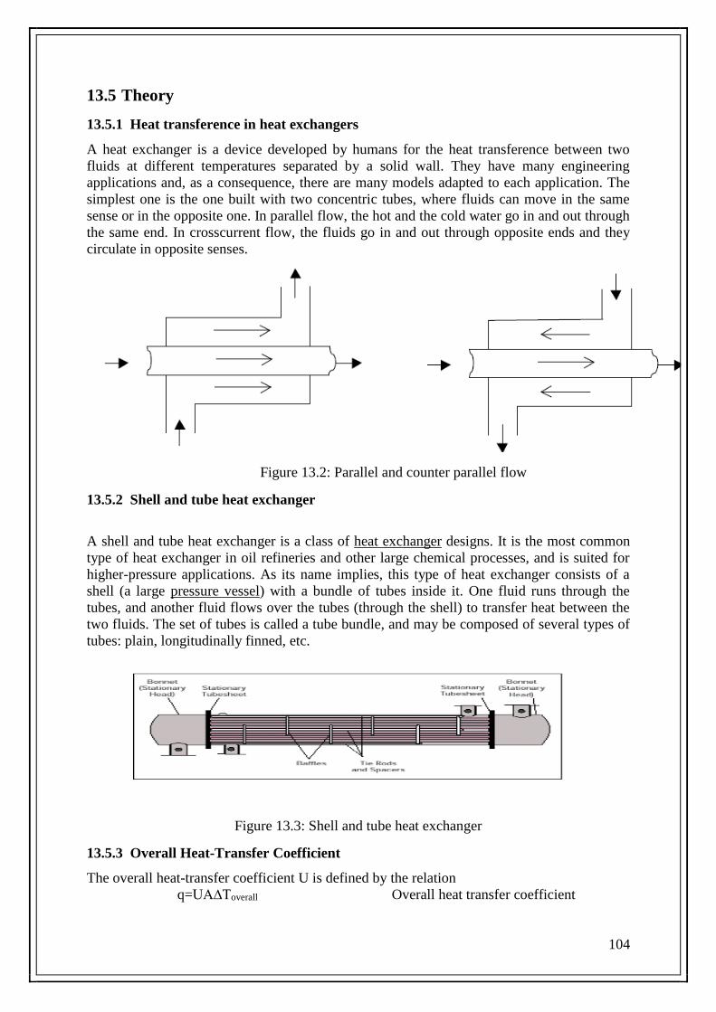
104
13.5 Theory
13.5.1 Heat transference in heat exchangers
A heat exchanger is a device developed by humans for the heat transference between two
fluids at different temperatures separated by a solid wall. They have many engineering
applications and, as a consequence, there are many models adapted to each application. The
simplest one is the one built with two concentric tubes, where fluids can move in the same
sense or in the opposite one. In parallel flow, the hot and the cold water go in and out through
the same end. In crosscurrent flow, the fluids go in and out through opposite ends and they
circulate in opposite senses.
Figure 13.2: Parallel and counter parallel flow
13.5.2 Shell and tube heat exchanger
A shell and tube heat exchanger is a class of heat exchanger designs. It is the most common
type of heat exchanger in oil refineries and other large chemical processes, and is suited for
higher-pressure applications. As its name implies, this type of heat exchanger consists of a
shell (a large pressure vessel) with a bundle of tubes inside it. One fluid runs through the
tubes, and another fluid flows over the tubes (through the shell) to transfer heat between the
two fluids. The set of tubes is called a tube bundle, and may be composed of several types of
tubes: plain, longitudinally finned, etc.
Figure 13.3: Shell and tube heat exchanger
13.5.3 Overall Heat-Transfer Coefficient
The overall heat-transfer coefficient U is defined by the relation
q=UA∆Toverall Overall heat transfer coefficient

105
Although final heat-exchanger designs will be made on the basis of careful calculations of U,
it is helpful to have a tabulation of values of the overall heat-transfer coefficient for various
situations that may be encountered in practice
13.5.4 The Log Mean Temperature Difference (LMTD)
Being ∆T1 = Th,i - Tc,i and ∆T2 = Th,o - Tc,o in parallel flow
∆T1 = Th,i - Tc,o and ∆T2 = Th,o - Tc,i in countercurrent flow.
Tlm=(∆T1)−(∆T2)
ln [∆T1
∆T2]
13.5.5 Effectiveness-Ntu Method
Effectiveness= Actual heat transfer
Maximum possible heat transfer
13.5.6 Capacity coefficient
Capacity coefficient will be defined as (CR)
Cr=𝐶𝑚𝑖𝑛
𝐶𝑚𝑎𝑥=……….
w/k
w/k
Mass flow rate multiplied by specific heat) Ch and Cc for the hot and cold fluids respectively,
and denoting the smaller one as C min
13.5.7 Reynolds number
In fluid mechanics, the Reynolds number (Re) is a dimensionless quantity that is used to help
predict similar flow patterns in different fluid flow situations. The Reynolds number is
defined as the ratio of momentum forces to viscous forces and consequently quantifies the
relative importance of these two types of forces for given flow conditions. They are also used
to characterize different flow regimes within a similar fluid, such as laminar or turbulent flow
3) Laminar flow occurs at low Reynolds numbers, where viscous forces are dominant,
and is characterized by smooth, constant fluid motion;
4) Turbulent flow occurs at high Reynolds numbers and is dominated by inertial forces,
which tend to produce chaotic eddies, vortices and other flow instabilities.
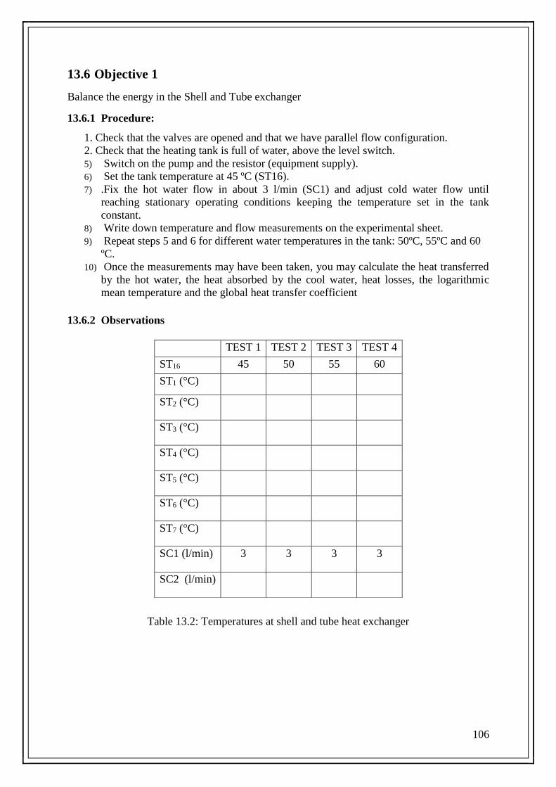
106
13.6 Objective 1
Balance the energy in the Shell and Tube exchanger
13.6.1 Procedure:
1. Check that the valves are opened and that we have parallel flow configuration.
2. Check that the heating tank is full of water, above the level switch.
5) Switch on the pump and the resistor (equipment supply).
6) Set the tank temperature at 45 ºC (ST16).
7) .Fix the hot water flow in about 3 l/min (SC1) and adjust cold water flow until
reaching stationary operating conditions keeping the temperature set in the tank
constant.
8) Write down temperature and flow measurements on the experimental sheet.
9) Repeat steps 5 and 6 for different water temperatures in the tank: 50ºC, 55ºC and 60
ºC.
10) Once the measurements may have been taken, you may calculate the heat transferred
by the hot water, the heat absorbed by the cool water, heat losses, the logarithmic
mean temperature and the global heat transfer coefficient
13.6.2 Observations
Table 13.2: Temperatures at shell and tube heat exchanger
TEST 1 TEST 2 TEST 3 TEST 4
ST16 45 50 55 60
ST1 (°C)
ST2 (°C)
ST3 (°C)
ST4 (°C)
ST5 (°C)
ST6 (°C)
ST7 (°C)
SC1 (l/min) 3 3 3 3
SC2 (l/min)
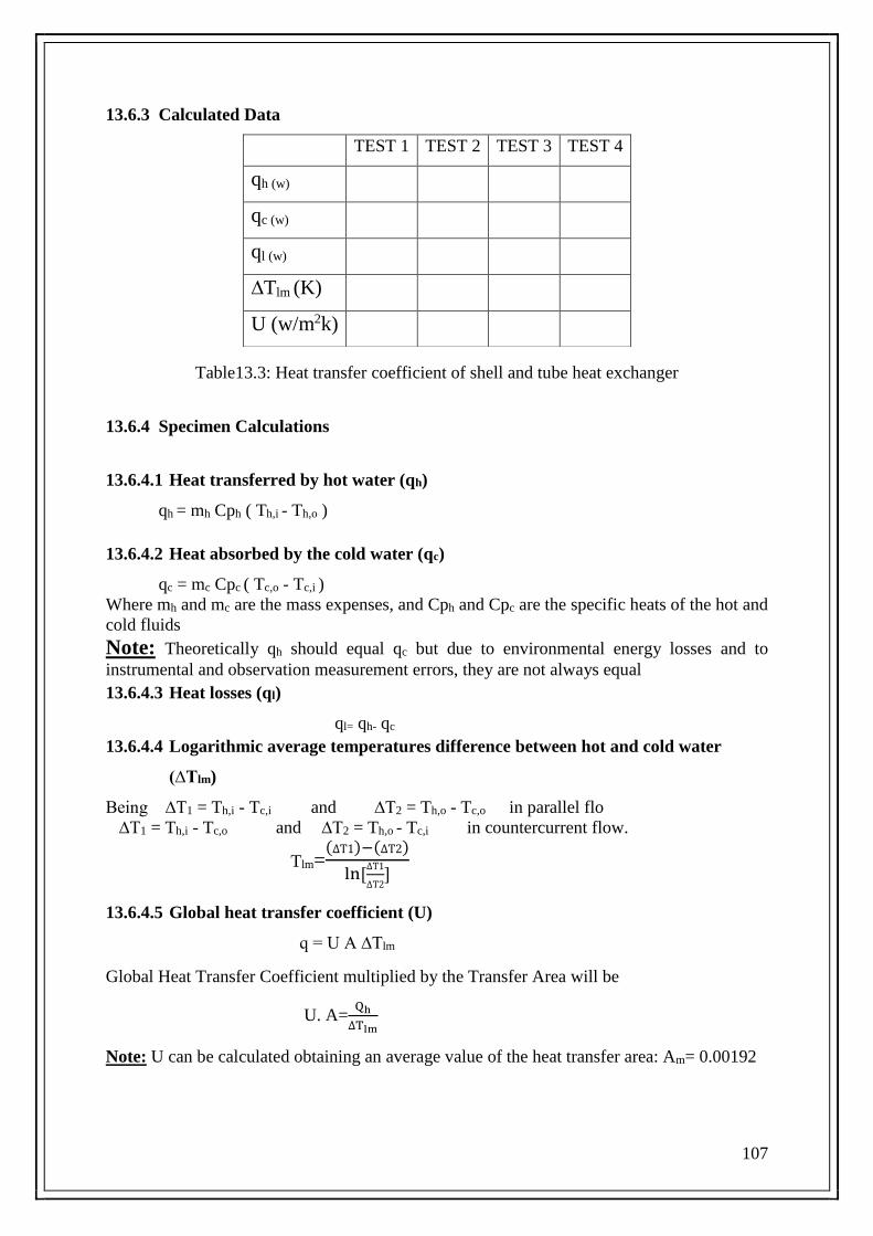
107
13.6.3 Calculated Data
Table13.3: Heat transfer coefficient of shell and tube heat exchanger
13.6.4 Specimen Calculations
13.6.4.1 Heat transferred by hot water (qh)
qh = mh Cph ( Th,i - Th,o )
13.6.4.2 Heat absorbed by the cold water (qc)
qc = mc Cpc ( Tc,o - Tc,i )
Where mh and mc are the mass expenses, and Cph and Cpc are the specific heats of the hot and
cold fluids
Note: Theoretically qh should equal qc but due to environmental energy losses and to
instrumental and observation measurement errors, they are not always equal
13.6.4.3 Heat losses (ql)
ql= qh- qc
13.6.4.4 Logarithmic average temperatures difference between hot and cold water
(∆Tlm)
Being ∆T1 = Th,i - Tc,i and ∆T2 = Th,o - Tc,o in parallel flo
∆T1 = Th,i - Tc,o and ∆T2 = Th,o - Tc,i in countercurrent flow.
Tlm=(∆T1)−(∆T2)
ln [∆T1
∆T2]
13.6.4.5 Global heat transfer coefficient (U)
q = U A ∆Tlm
Global Heat Transfer Coefficient multiplied by the Transfer Area will be
U. A=Qh
∆Tlm
Note: U can be calculated obtaining an average value of the heat transfer area: Am= 0.00192
TEST 1 TEST 2 TEST 3 TEST 4
qh (w)
qc (w)
ql (w)
∆Tlm (K)
U (w/m2k)

108
13.7 Objective 2
Calculate the heat exchanger effectiveness by NTU method.
13.7.1 Procedure
1. Check that the valves are opened and that we have countercurrent flow configuration.
2. Check that the heating tank is filled with water above the level switch.
3. Switch on the pump and the resistor (equipment supply).
4. Set the tank temperature in 60 ºC (ST16).
5. Fix the hot water flow in 3 l/min approx. (SC1) and adjust cold water flow to reach
stationary operating conditions, keeping constant temperatures set for the tank.
6. Write down the temperature and flow measurements on the experimental sheet.
7. Set the valves appropriately in order to invert cold water flow direction to produce a
parallel flow configuration.
8. Make sure that 60ºC temperatures are kept in the tank and that the same hot and cold water
flows set in step 5 are also maintained.
9. Once the system is stabilized, write down the temperature measurements and flow values
on the experimental sheet.
10. Once the measurements have been taken, calculate the experimental effectiveness, the
theoretical effectiveness by the NTU method and the theoretical temperatures at the
exchanger outlet.
13.7.2 Observations
Table 13.4: Temperatures for shell and tube heat exchanger
TEST 1 TEST 2
ST16 45 50
ST1 (°C)
ST2 (°C)
ST3 (°C)
ST4 (°C)
ST5 (°C)
ST6 (°C)
ST7 (°C)
SC1 (l/min) 3 3
SC2 (l/min)

109
13.7.3 Calculated Data
Table 13.5: Effectiveness of shell and tube heat exchanger
13.7.4 Specimen Calculations
13.7.4.1 Experimental effectiveness (ϵ)
The effectiveness is the quotient between the heat really exchanged and the maximum heat
that could be transferred in an infinite area exchanger in a crosscurrent flow.
If mhCph˂mcCpc ϵ=(Th,i)−(Th,o)
Th,i−Tc,o
mhCph ˃mcCpc ϵ=(Tc,o)−(Tc,i)
Th,i−Tc,i
13.7.4.2 Logarithmic average temperatures difference between hot and cold water
(∆Tlm)
Being ∆T1 = Th,i - Tc,i and ∆T2 = Th,o - Tc,o in parallel flow
∆T1 = Th,i - Tc,o and ∆T2 = Th,o - Tc,i in countercurrent flow.
Tlm=(∆T1)−(∆T2)
ln [∆T1
∆T2]
13.7.4.3 Global heat transfer coefficient (U)
q = U A ∆Tlm
Global Heat Transfer Coefficient multiplied by the Transfer Area will be
U. A=Qh
∆Tlm
13.7.4.4 Number of transmission units
NTU=U.A
(m.Cp)min
TEST 1
Crosscurrent Flow
TEST 2
Parallel flow
ϵ
qh (w)
∆Tlm (K)
U.A (w/k)
NTU
CR
ϵNTU

110
13.7.4.5 Capacity coefficient
Capacity coefficient is determined by
Cr=mCpmin
mCpmax=……….
w/k
w/k
Once the NTU and Cr are obtained, we can calculate the effectiveness, but depending if the
flow is in crosscurrent or in parallel flow, we will have to use different expressions
13.7.4.6 Temperatures at the exchanger outlet
ϵNTU=1−e−NTU.(1+CR)
1+CR For Parallel flow
ϵNTU=1−e−NTU.(1−CR)
1−CR× e−NTU.(1−CR) For Crosscurrent flow
13.8 Statistical Analysis
For overall heat transfer coefficient “U”
1) xavg= x1+x2+x3
n
2) Sx=√1
𝑛−1((𝑥1 − 𝑥𝑎𝑣𝑔)2 + (𝑥2 − 𝑥𝑎𝑣𝑔)2 + (𝑥3 − 𝑥𝑎𝑣𝑔)2)
13.9 Conclusion
13.10 Questions
1) What is the difference between the temperature distribution for parallel and
crosscurrent flow in shell and tube heat exchanger
2) What is Global heat transference coefficient
3) What is Logarithmic temperatures mean difference
4) What is difference of shell and tube heat exchanger from other heat exchangers
13.11 Comments

111
14. LAB SESSION 14
To calculate logarithmic mean temperature difference (LMTD) and global heat transfer
coefficient of plate heat exchanger
14.1 Learning Objective
Balance the energy in the Shell and Tube exchanger
14.2 Apparatus
EDIBON’s TIPL Plate Heat Exchanger (Serial No= TIPL 0047/11)
14.3 Main Parts
14.4 Useful Data
14.4.1 BASE UNIT
Net weight: 30 kg.
Height: 400 mm
Width: 1000 mm
Depth: 500 mm
14.4.2 Heat Exchanger
Net weight: 20 kg.
Height: 300 mm
Width: 1000 mm
Depth: 500 mm
Maximum Flow 12m3/h
Max. Work Pressure 10bar
Max. Work Temperature 100ºC
Minimum. Work Temperature 0ºC
Maximum number of plates 10
IDENTIFICATION DESCRIPTION
ST-16 Water Tank Temperature Sensor
ST-1 Cold Water Temperature Sensor at the inlet/Outlet of the exchanger
ST-2 Hot Water Temperature sensor at the inlet of the exchanger
ST-3 Cold Water Temperature sensor at the inlet/outlet of the exchanger
ST-4 Hot Water Temperature sensor at the outlet of the exchanger
SC-1 Hot water flow sensor
SC-2 Cold water flow sensor
AVR-1 Hot water flow regulation valve.
AVR-2 Cold water flow regulation valve
AN-1 Water level switch of the tank
AR-1 Electric resistance
AB-1 Hot Water Flow Centrifugal Pump
AV-2,AV-3, AV-4 Y
AV-5
Ball valves of the cold water circuit for setting parallel or counter
current flow
AV-1,AV-6, AV-
7 and AV-8
Ball valves for draining the pipes
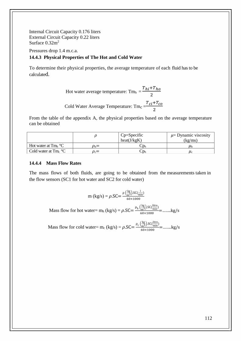
112
Internal Circuit Capacity 0.176 liters
External Circuit Capacity 0.22 liters
Surface 0.32m2
Pressures drop 1.4 m.c.a.
14.4.3 Physical Properties of The Hot and Cold Water
To determine their physical properties, the average temperature of each fluid has to be
calculated.
Hot water average temperature: Tmh = 𝑇ℎ𝑖+𝑇ℎ𝑜
2
Cold Water Average Temperature: Tmc =𝑇𝑐𝑖+𝑇𝑐𝑜
2
From the table of the appendix A, the physical properties based on the average temperature
can be obtained
14.4.4 Mass Flow Rates
The mass flows of both fluids, are going to be obtained from the measurements taken in
the flow sensors (SC1 for hot water and SC2 for cold water)
m (kg/s) = 𝜌.SC= ρ (
kg
m3).SC(l
min)
60×1000
Mass flow for hot water= mh (kg/s) = 𝜌.SC= ρh (
kg
m3).SC(litre
min)
60×1000=……..kg/s
Mass flow for cold water= mc (kg/s) = 𝜌.SC= ρc (
kg
m3).SC(litre
min)
60×1000=……..kg/s
𝜌 Cp=Specific
heat(J/kgK) 𝜇= Dynamic viscosity
(kg/ms)
Hot water at Tmh °C 𝜌h= Cph 𝜇h
Cold water at Tmc °C 𝜌c= Cph 𝜇c
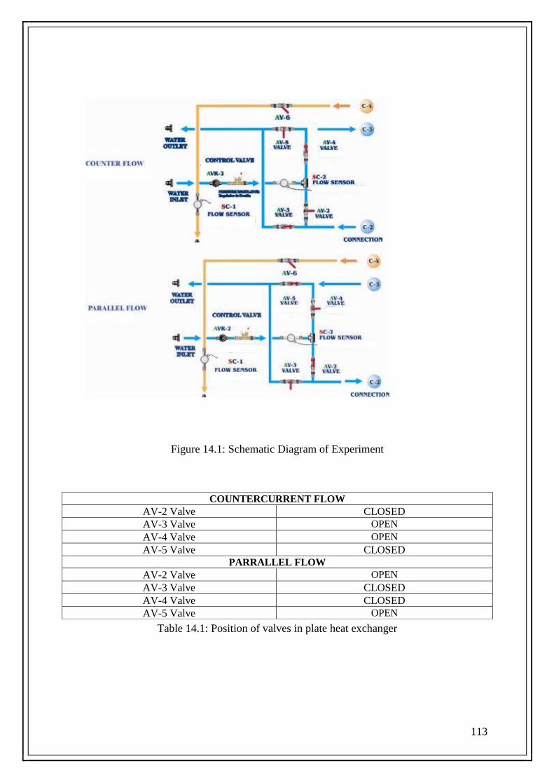
113
Figure 14.1: Schematic Diagram of Experiment
Table 14.1: Position of valves in plate heat exchanger
COUNTERCURRENT FLOW
AV-2 Valve CLOSED
AV-3 Valve OPEN
AV-4 Valve OPEN
AV-5 Valve CLOSED
PARRALLEL FLOW
AV-2 Valve OPEN
AV-3 Valve CLOSED
AV-4 Valve CLOSED
AV-5 Valve OPEN
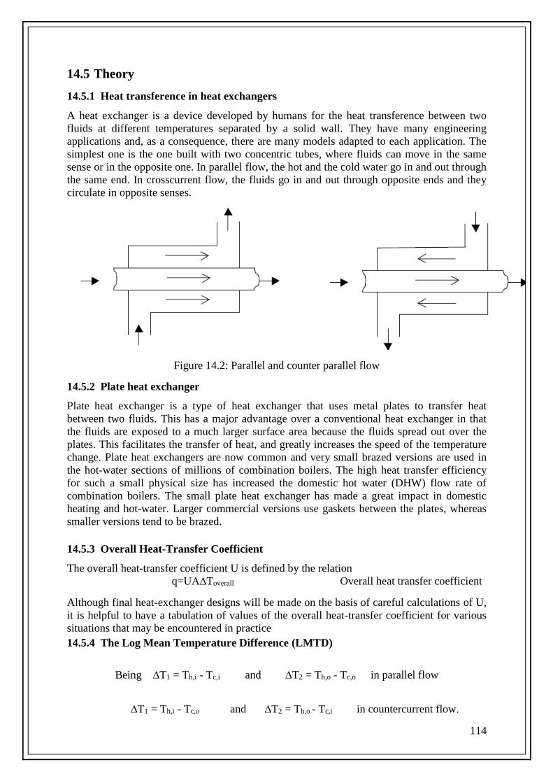
114
14.5 Theory
14.5.1 Heat transference in heat exchangers
A heat exchanger is a device developed by humans for the heat transference between two
fluids at different temperatures separated by a solid wall. They have many engineering
applications and, as a consequence, there are many models adapted to each application. The
simplest one is the one built with two concentric tubes, where fluids can move in the same
sense or in the opposite one. In parallel flow, the hot and the cold water go in and out through
the same end. In crosscurrent flow, the fluids go in and out through opposite ends and they
circulate in opposite senses.
Figure 14.2: Parallel and counter parallel flow
14.5.2 Plate heat exchanger
Plate heat exchanger is a type of heat exchanger that uses metal plates to transfer heat
between two fluids. This has a major advantage over a conventional heat exchanger in that
the fluids are exposed to a much larger surface area because the fluids spread out over the
plates. This facilitates the transfer of heat, and greatly increases the speed of the temperature
change. Plate heat exchangers are now common and very small brazed versions are used in
the hot-water sections of millions of combination boilers. The high heat transfer efficiency
for such a small physical size has increased the domestic hot water (DHW) flow rate of
combination boilers. The small plate heat exchanger has made a great impact in domestic
heating and hot-water. Larger commercial versions use gaskets between the plates, whereas
smaller versions tend to be brazed.
14.5.3 Overall Heat-Transfer Coefficient
The overall heat-transfer coefficient U is defined by the relation
q=UA∆Toverall Overall heat transfer coefficient
Although final heat-exchanger designs will be made on the basis of careful calculations of U,
it is helpful to have a tabulation of values of the overall heat-transfer coefficient for various
situations that may be encountered in practice
14.5.4 The Log Mean Temperature Difference (LMTD)
Being ∆T1 = Th,i - Tc,i and ∆T2 = Th,o - Tc,o in parallel flow
∆T1 = Th,i - Tc,o and ∆T2 = Th,o - Tc,i in countercurrent flow.

115
Tlm=(∆T1)−(∆T2)
ln [∆T1
∆T2]
The Log Mean Temperature Difference
14.6 Objective
Balance the energy in the Shell and Tube exchanger
14.6.1 Procedure
1. Verify that valves are opened and that parallel flow configuration has been set.
2. Verify that the heating tank is filled with water over the level switch.
3. Turn on the pump and the resistance (the equipment power supply).
4. Set the tank temperature in 50ºC (ST16).
5. Set the hot water flow in 3 l/min approx. (SC1) and adjust the cold water flow so stationary
operating conditions may be reached keeping the temperature in the tank constant
6. Write down temperature and flow measurements on the experimental sheet.
7. Repeat steps 5 and 6 for different temperatures of the water tank: 55ºC, 60ºC and 65ºC.
8. Once the measurements have been taken you may calculate the heat transferred by the hot
water, the heat absorbed by the cold water, heat losses, the logarithmic average temperatures
difference and the heat transfer global coefficient
14.6.2 Observations
Table 14.2: Temperatures of Plate Heat Exchangers
TEST 1 TEST 2 TEST 3 TEST 4
ST16 50 55 60 65
ST1 (°C)
ST2 (°C)
ST3 (°C)
ST4 (°C)
SC1 (l/min) 3 3 3 3
SC2 (l/min)
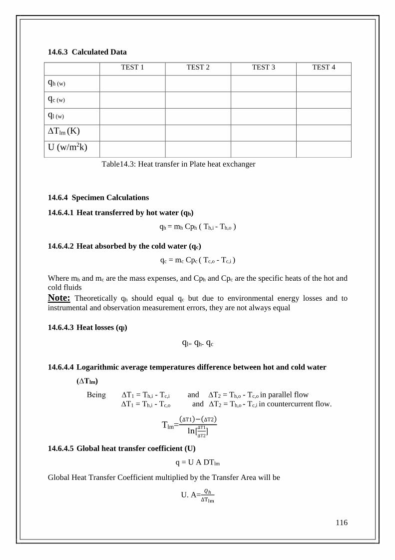
116
14.6.3 Calculated Data
Table14.3: Heat transfer in Plate heat exchanger
14.6.4 Specimen Calculations
14.6.4.1 Heat transferred by hot water (qh)
qh = mh Cph ( Th,i - Th,o )
14.6.4.2 Heat absorbed by the cold water (qc)
qc = mc Cpc ( Tc,o - Tc,i )
Where mh and mc are the mass expenses, and Cph and Cpc are the specific heats of the hot and
cold fluids
Note: Theoretically qh should equal qc but due to environmental energy losses and to
instrumental and observation measurement errors, they are not always equal
14.6.4.3 Heat losses (ql)
ql= qh- qc
14.6.4.4 Logarithmic average temperatures difference between hot and cold water
(∆Tlm)
Being ∆T1 = Th,i - Tc,i and ∆T2 = Th,o - Tc,o in parallel flow
∆T1 = Th,i - Tc,o and ∆T2 = Th,o - Tc,i in countercurrent flow.
Tlm=(∆T1)−(∆T2)
ln [∆T1
∆T2]
14.6.4.5 Global heat transfer coefficient (U)
q = U A DTlm
Global Heat Transfer Coefficient multiplied by the Transfer Area will be
U. A=𝑄ℎ
∆Tlm
TEST 1 TEST 2 TEST 3 TEST 4
qh (w)
qc (w)
ql (w)
∆Tlm (K)
U (w/m2k)

117
Note: U can be calculated obtaining an average value of the heat transfer area: Am= 0.192
14.7 Graph
Represent the temperature distribution in counter-current and parallel flow configurations.
For that purpose, represent hot and cold water temperature values in ºC (T) on the vertical
axis; and the position along the exchanger in meters on the horizontal axis. You should
consider the length of the exchanger to be 0.5m and that we have three measure points.
14.8 Statistical Analysis
For overall heat transfer coefficient “U”
1) xavg= x1+x2+x3
n
2) Sx=√1
𝑛−1((𝑥1 − 𝑥𝑎𝑣𝑔)2 + (𝑥2 − 𝑥𝑎𝑣𝑔)2 + (𝑥3 − 𝑥𝑎𝑣𝑔)2)
14.9 Conclusion
14.10 Questions
1) What is the difference between the temperature distribution for parallel and
crosscurrent flow in Plate heat exchanger
2) What is Global heat transference coefficient
3) What is Logarithmic temperatures mean difference
4) What is difference of Plate heat exchanger from other heat exchangers
14.11 Comments
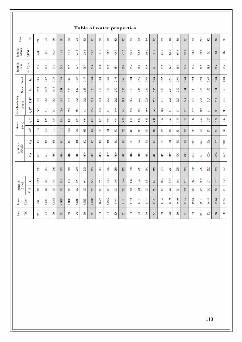
118

119