Full Terms & Conditions of access and use can be found athttp://www.tandfonline.com/action/journalInformation?journalCode=nmcm20

Download by: [TU Wien University Library] Date: 01 August 2017, At: 04:05

Mathematical and Computer Modelling of DynamicalSystemsMethods, Tools and Applications in Engineering and Related Sciences

ISSN: 1387-3954 (Print) 1744-5051 (Online) Journal homepage: http://www.tandfonline.com/loi/nmcm20

Heat capacity and heat transfer coefficientestimation for a dynamic thermal model of railvehicles

Raphael N. Hofstädter, Thomas Zero, Christian Dullinger, Gregor Richter &Martin Kozek

To cite this article: Raphael N. Hofstädter, Thomas Zero, Christian Dullinger, Gregor Richter &Martin Kozek (2017) Heat capacity and heat transfer coefficient estimation for a dynamic thermalmodel of rail vehicles, Mathematical and Computer Modelling of Dynamical Systems, 23:5,439-452, DOI: 10.1080/13873954.2016.1263670

To link to this article: http://dx.doi.org/10.1080/13873954.2016.1263670

Published online: 05 Dec 2016.

Submit your article to this journal

Article views: 39

View related articles

View Crossmark data

Heat capacity and heat transfer coefficient estimation for adynamic thermal model of rail vehiclesRaphael N. Hofstädtera, Thomas Zerob, Christian Dullingera, Gregor Richterb

and Martin Kozeka

aInstitute of Mechanics and Mechatronics, Vienna University of Technology, Vienna, Austria; bRTA – Rail TecArsenal Fahrzeugversuchsanlage GmbH, Vienna, Austria

ABSTRACTThis paper provides a method for estimating the parameters of a dynamicthermal rail vehicle model and reference values of these parameters. Alinear dynamic discrete time system is used to model the thermal behaviourof the vehicle relevant for thermal comfort and air conditioning. The heatcapacities and the heat transfer coefficients are stated for various vehicleclasses. While dynamic thermal models are state of the art in buildings, carsand rail vehicles, no reference values can be found for these parameters.This paper shows how to estimate the heat capacity and the heat transfercoefficient from measured data for a given thermal model structure. Twodifferent measurement data sources are used: special experiments andexisting measurements. While specially designed experiments are onlypossible for new measurements, it is shown that satisfying results can beobtained with existing measurements. Measurement data from 13 vehiclesare used to provide reference values for all passenger vehicles classes: tram,metro, regional and main-line. If all assumptions are satisfied, simulationresults of the indoor air temperature agree well with measurements.Reference values for parameters of a dynamic thermal model are thebasis for a wide application of such models in the rail vehicle industry.

ARTICLE HISTORYReceived 25 January 2015Accepted 17 November 2016

KEYWORDSThermal model; parameterestimation; heat capacity;heat transfer coefficient; railvehicle

1. Introduction

Rail vehicles are the back bone of short-distance public transport (SDPT). In a large city likeVienna, the percentage of SDPT (including buses) is already at 35% [1]. As a result, the localoperator serves, after own states, 2.5 million passengers per day [2]. Like every other industrialsector, the rail vehicle industry is subject to constant change. Since the 1950s, one of the keytrends is the occurring urbanization which leads to a growth of cities and urban centres. By 2050,84% of the European population will live in urban areas [3].

As a result, the requirements of the population for mobility will increase in number andcomplexity. In order to sustain this growth, transport should mainly be covered by SDPT. Theincreased energy costs and the effort to reduce CO2 emissions support the use of rail vehicles.Thus, Vienna clearly prioritizes public transport, walking and cycling over car traffic [4, p. 25].

In his seminal work, Struckl [5] made a life cycle analysis of the metro Oslo to demonstrateenergy saving potential for rail vehicles. About 30% of the total energy consumed is used fortemperature control of the vehicle during driving cycles of the considered metro [5, see Fig. 4.53].This magnitude is confirmed in [6]. In [7], it was measured that 11% of the total energy isconsumed during stabling hours. The significant energy consumption of heating, ventilation and

CONTACT Raphael N. Hofstädter r.hofstaedter@gmail.com© 2016 Informa UK Limited, trading as Taylor & Francis Group

MATHEMATICAL AND COMPUTER MODELLING OF DYNAMICAL SYSTEMS, 2017VOL. 23, NO. 5, 439–452https://doi.org/10.1080/13873954.2016.1263670

air condition (HVAC) systems calls for an efficient design of the related components. A funda-mental element of this task is a dynamic thermal model of rail vehicles.

For the calculation of the annual energy consumption of the HVAC [8] or other optimizationmeasures [9,10], a mathematical description of the considered system needs to be found andparameters of this system need to be identified.

1.1. Literature

Vehicles are usually air-conditioned by vapour compression refrigerators, although other methodsexist [11] and are applied in practice [12]. According to [13], there are three possibilities to modelHVAC systems: physics based, data driven or grey box. The very same principles can be applied tothermal models of (rail) vehicles.

Marcos et al. [14] developed and validated an analytical (physics-based) model of a car withtwo heat capacities. In [15], an analytical thermal model for an automotive vehicle is devel-oped and validated. Parameters were estimated analytically (physics based), e.g. the heatcapacity of the car was multiplied by the mass and the average specific heat capacity.Marachlian et al. [16] used an exergy-based numerical model to simulate the cars HVACoperations. Today, a thermal simulation software for automotive vehicles is already available[17] and used for the simulation of combined cooling loops [18]. The thermal behaviour ofbuildings can be simulated using a modular Modelica library [19]. In [20], dynamic coolingloads were studied using an analytical thermal model of a Chinese main-line train. Anotherdynamic thermal model of an urban rail vehicle is part of previous works of some of theauthors and can be found in [21]. An analytical simulation model was also used by Li and Sun[22] to simulate and analyse the entire system of air conditioning unit and passenger room.All thermal vehicle simulation approaches are almost exclusively used for only one specificvehicle. The models that use an analytical approach are purposeful, but it is time consumingto determine every necessary parameter. For industrial practices, it would be advantageous ifbenchmarks or reference values for a dynamic thermal simulation model were available.Measurement data should be sufficiently available, because thermal tests of rail vehicles canlook back on a long history.

Function tests have been conducted for rail vehicles in Vienna since 1958. Especially refriger-ated wagons were examined back then and their heat transfer coefficient (k value) was measured.Over the years, testing was expanded to passenger trains and metros. Nowadays, function tests ina climatic wind tunnel (CWT) are part of standard commissioning. Since these tests are con-sidered during construction of the vehicle, lower k values are intended. The k value of the vehiclesis usually measured during these tests [23], according to European Standards [24,25]. These testsare done to keep operational costs low and availability high [26,27]. Although unpublishedrecords about the identification of the heat capacity can be traced back until the 60s, no generallyaccepted procedures or regulations exist for the estimation.

In building technologies an obligatory holistic examination of buildings, in terms of energyefficiency, was introduced [28] by a new EU directive [29] and national law [30]. However, nostandards exist for model structure and parameter choice of dynamic thermal models of railvehicles’ eigen behaviour. This paper is a step forward and provides a compact yet versatile modelstructure and reference values of the thermal behaviour of the vehicle for different analytical–thermal models and for various types of rail vehicles (tram, metro, regional and main-line).

1.2. Contents

Different models that are describing the vehicles’ behaviour are derived from a general dynamicmodel in Section 2. Afterwards, the theoretical fundamentals and the practical requirements forthe conducted and available measurements are discussed in Section 3. All assumptions are

440 R. N. HOFSTÄDTER ET AL.

summarized in Section 4, and the used simulation model and the estimation method are describedin Section 5. In Section 6, the obtained results are shown and discussed.

2. Modelling

The modelling section summarizes the state of art for thermal modelling for rail vehicles andpresents a low-order dynamic model structure which can be efficiently parametrized.

2.1. Generic analytic–dynamic thermal model

Relevant variables for the thermal comfort inside the a rail vehicle are T the temperature of theindoor air and Y the absolute humidity of the indoor air, according to the current standards[24,25]. The air velocity is just defined as a constraint that must be satisfied and is usually onlyconsidered during design of the air distribution system.

The entire rail vehicle consists of N thermal system. Every system i of the rail vehicle can bedescribed individually. Equations for T and Y can be stated based on energy and mass balances forevery system i.

CidTi

dt¼ � _Qi; loss � _Qi; iþ1 þ _Qi; solar þ _Qi; pas þ _Qi; aux þ _Ei; sup � _Ei; exh (1)

mi � dYi

dt¼ _EWi; sup � _EWi; exh þ _EWi; pas þ _EWi; aux (2)

In Equation (1), Ci is the heat capacity associated with temperature Ti. _Qi; loss describes thedissipated heat from the component of the system with the temperature Ti to the environment._Qi; iþ1 is the energy flow between the components with temperatures Ti and Tiþ1, respectively._Qi; solar takes the solar radiation (direct and indirect) and _Qi; pas the dissipated sensible heat bypassengers into account. _Qi; aux is the heat dissipated by auxiliaries, i.e. electrical lighting andpassenger information system. _Ei; sup is the mass flow of supply air and _Ei; exh the mass flow ofexhaust air. In Equation (2), mi denotes the mass of the indoor air, _EWi; sup is the mass flow of waterin the supply air and _EWi; exh in the exhaust air, _EWi; pas is the dissipated water due to sensible heat ofpassengers and _EWi; aux is any further mass flow of water in Equation (2).

Only parameters Ci, mi and terms _Qi; loss and _Qi; iþ1 are necessary to describe the vehicles’behaviour. Since the initial analytical guess of mi, sufficed for the calculations of theabsolute humidity Y in previous works of some of the authors [31], this paper will focuson Ci and the terms _Qi; loss and _Qi; iþ1 for the calculations of the temperature(s) Ti. The airvolume of system i was multiplied by the air density to obtain the mass of indoor air mi.

Following subsections derive three vehicle models from the generic analytic–dynamic thermalmodel to describe the vehicles’ behaviour.

2.2. Second-order thermal vehicle model

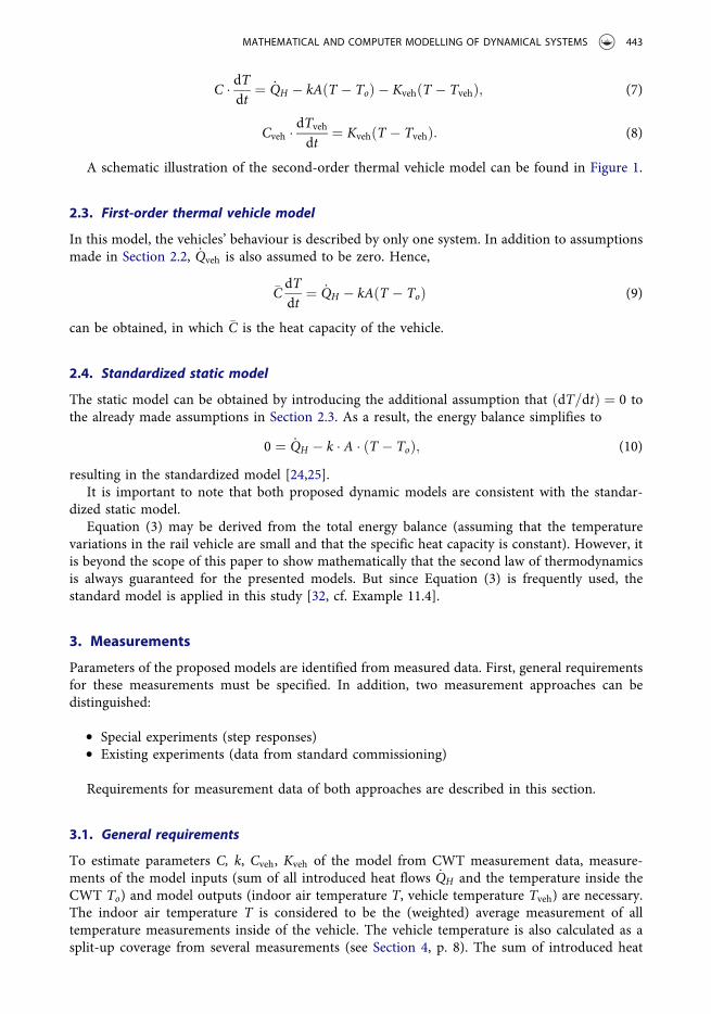
The vehicle is assumed to consist of two systems (N ¼ 2) with two heat capacities and twotemperatures, see Figure 1. The equation for system 1 (i ¼ 1) follows from Equation (1) bykeeping only terms relevant to the vehicles’ behaviour.

C1dT1

dt¼ � _Q1; loss � _Q1;2 þ _Q1; solar þ _Q1; pas þ _Q1; aux þ _E1; sup � _E1; exh|fflfflfflfflfflfflfflfflfflffl{zfflfflfflfflfflfflfflfflfflffl}

_QH

In Figure 1, it is shown that HVAC ports are sealed. So, _E1; sup and _E1; exh need to bereplaced by _QH during measurements (see Section 3) which holds the sum of all introduced

MATHEMATICAL AND COMPUTER MODELLING OF DYNAMICAL SYSTEMS 441

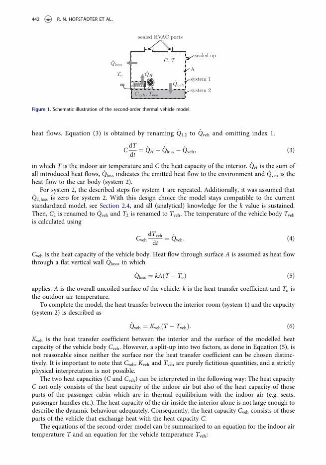
heat flows. Equation (3) is obtained by renaming _Q1;2 to _Qveh and omitting index 1.

CdTdt

¼ _QH � _Qloss � _Qveh; (3)

in which T is the indoor air temperature and C the heat capacity of the interior. _QH is the sum ofall introduced heat flows, _Qloss indicates the emitted heat flow to the environment and _Qveh is theheat flow to the car body (system 2).

For system 2, the described steps for system 1 are repeated. Additionally, it was assumed that_Q2; loss is zero for system 2. With this design choice the model stays compatible to the currentstandardized model, see Section 2.4, and all (analytical) knowledge for the k value is sustained.Then, C2 is renamed to _Qveh and T2 is renamed to Tveh. The temperature of the vehicle body Tveh

is calculated using

CvehdTveh

dt¼ _Qveh: (4)

Cveh is the heat capacity of the vehicle body. Heat flow through surface A is assumed as heat flowthrough a flat vertical wall _Qloss, in which

_Qloss ¼ kA T � Toð Þ (5)

applies. A is the overall uncoiled surface of the vehicle. k is the heat transfer coefficient and To isthe outdoor air temperature.

To complete the model, the heat transfer between the interior room (system 1) and the capacity(system 2) is described as

_Qveh ¼ Kveh T � Tvehð Þ: (6)

Kveh is the heat transfer coefficient between the interior and the surface of the modelled heatcapacity of the vehicle body Cveh. However, a split-up into two factors, as done in Equation (5), isnot reasonable since neither the surface nor the heat transfer coefficient can be chosen distinc-tively. It is important to note that Cveh, Kveh and Tveh are purely fictitious quantities, and a strictlyphysical interpretation is not possible.

The two heat capacities (C and Cveh) can be interpreted in the following way: The heat capacityC not only consists of the heat capacity of the indoor air but also of the heat capacity of thoseparts of the passenger cabin which are in thermal equilibrium with the indoor air (e.g. seats,passenger handles etc.). The heat capacity of the air inside the interior alone is not large enough todescribe the dynamic behaviour adequately. Consequently, the heat capacity Cveh consists of thoseparts of the vehicle that exchange heat with the heat capacity C.

The equations of the second-order model can be summarized to an equation for the indoor airtemperature T and an equation for the vehicle temperature Tveh:

sealed HVAC ports

sealed opC, T

Cveh, Tveh

To

Qloss

QH

Qveh

system 2

system 1

A

Figure 1. Schematic illustration of the second-order thermal vehicle model.

442 R. N. HOFSTÄDTER ET AL.

C � dTdt

¼ _QH � kA T � Toð Þ � Kveh T � Tvehð Þ; (7)

Cveh � dTveh

dt¼ Kveh T � Tvehð Þ: (8)

A schematic illustration of the second-order thermal vehicle model can be found in Figure 1.

2.3. First-order thermal vehicle model

In this model, the vehicles’ behaviour is described by only one system. In addition to assumptionsmade in Section 2.2, _Qveh is also assumed to be zero. Hence,

�CdTdt

¼ _QH � kA T � Toð Þ (9)

can be obtained, in which �C is the heat capacity of the vehicle.

2.4. Standardized static model

The static model can be obtained by introducing the additional assumption that dT=dtð Þ ¼ 0 tothe already made assumptions in Section 2.3. As a result, the energy balance simplifies to

0 ¼ _QH � k � A � T � Toð Þ; (10)

resulting in the standardized model [24,25].It is important to note that both proposed dynamic models are consistent with the standar-

dized static model.Equation (3) may be derived from the total energy balance (assuming that the temperature

variations in the rail vehicle are small and that the specific heat capacity is constant). However, itis beyond the scope of this paper to show mathematically that the second law of thermodynamicsis always guaranteed for the presented models. But since Equation (3) is frequently used, thestandard model is applied in this study [32, cf. Example 11.4].

3. Measurements

Parameters of the proposed models are identified from measured data. First, general requirementsfor these measurements must be specified. In addition, two measurement approaches can bedistinguished:

● Special experiments (step responses)● Existing experiments (data from standard commissioning)

Requirements for measurement data of both approaches are described in this section.

3.1. General requirements

To estimate parameters C, k, Cveh, Kveh of the model from CWT measurement data, measure-ments of the model inputs (sum of all introduced heat flows _QH and the temperature inside theCWT To) and model outputs (indoor air temperature T, vehicle temperature Tveh) are necessary.The indoor air temperature T is considered to be the (weighted) average measurement of alltemperature measurements inside of the vehicle. The vehicle temperature is also calculated as asplit-up coverage from several measurements (see Section 4, p. 8). The sum of introduced heat

MATHEMATICAL AND COMPUTER MODELLING OF DYNAMICAL SYSTEMS 443

flows _QH is calculated both from the absorbed electrical power of the heater coils and theabsorbed electrical power of the fans.

Measurements need to be recorded with an adequately high sampling rate. The typically usedsampling rate of 10–1 min is sufficient. Since only the vehicles’ behaviour should be measured, allother influences and disturbances, as shown in Equations (1) and (2), should be eliminated in theCWT as well as possible. The simulated wind speed should be kept constant, the simulatedpassenger load _Qpas, the solar radiation _Qsolar and additional auxiliaries _Qaux must be turned off.All openings _Eexh and HVAC ports _Esup are sealed, as shown in Figure 1.

3.2. Special experiments

Due to economical limitations, two step tests are conducted with different signs. Initial conditionsshould be well defined and known. Due to the fact that the measurement of the vehicletemperature is difficult, it is desirable that the vehicle temperature Tveh and the indoor airtemperature T are constant at the beginning of the experiment.

Based on this state, one input is changed stepwise. At time t ¼ 0 the supplied heat flow isswitched to the value that follows from the expected k value. Usually, a rough estimate isknown, because it is analytically calculated by the manufacturer or a maximum permissiblevalue can be found in the standards for the vehicle class [24,25]. The experiment is conducteduntil a new steady state follows, i.e. the derivative of the indoor air temperature T and thedeviations of the vehicle temperature Tveh are almost zero. To reduce the necessary experi-ment time the experiment can be stopped earlier, if the final value can be estimated frommeasurement data and 95% of the step response has already been achieved. The step experi-ment is then repeated with reversed sign. After the experiment ends the initial conditionsshould be reached again.

3.3. Existing measurements

The procedure described for special experiments cannot be applied to historic measurements andthey cannot be repeated at justifiable cost. However, in the conducted measurements similarsections to the proposed special experiments can usually be found. These can also be used forparameter estimation, but not with the same accuracy. This includes the following experimenttypes:

● Pre-heating experiments of the vehicle using HVAC (pre-heating).● Measurement of the heat transfer coefficient (k value).● Cool down experiment (freezing test). The vehicle is allowed to cool down for 12 h.

The pre-heating and cool down experiment have the disadvantage that the introducedheat flow was not directly measured. Although it can be calculated from the measured airflow, the result is always subject to increased uncertainty. The measurement for estimatingthe heat transfer coefficient is almost always performed, though according to differentstandards.

This means that relevant parameters can typically be estimated with experiments for themeasurement of the heat transfer coefficient, as well as the conducted preparation and post-processing experiments before and afterwards. Figure 2 compares the existing measurementswith the special experiments. In the special experiments, only one input is changed at atime. First, the temperature inside the CWT is set, a steady state is awaited and then _QH ischanged.

444 R. N. HOFSTÄDTER ET AL.

4. Assumptions

The following assumptions have been made for the estimation of parameters:

● Ideal mixing: In the model, it is assumed that the air in the interior of the vehicle is ideallymixed. For the k-value experiments, this is ensured by temporary installed fans inside thevehicle.

● No heat transfer between outdoor air and heat capacity: The heat transfer between outdoorair and modelled heat capacity of the vehicle is neglected. For all considered vehicles belowthis is satisfied.

● Measurement of the temperature of the vehicle’s heat capacity: As measurement value for thetemperature of the vehicle’s heat capacity, the mean surface temperature of different surfacesinside the vehicle is used. All other considered metering points were not accessible formeasurement.

● Identification: An initial value must be given for identification. To estimate an accurateinitial value, a steady state is advantageous; unfortunately, this state is not always available.Therefore, some experiments could not be used for identification (see Table 1).

● Linear model: The proposed model for identification is linear in its parameters. Althoughnon-linear behaviour is observed in measurement data, the linear model fit is consideredsatisfying.

The simulation model and the estimated parameters from the measured data are only valid, ifthese assumptions are met.

5. Parameter estimation

The dynamic models, described in Section 2, are transformed to an explicit linear state spacerepresentation. To ensure compliance with the current standardized method, the k value isestimated accordingly. Afterwards, an assumption is made for the model structure by determiningthe noise model and the prediction error method (PEM) is used to estimate these parameters[33,34].

measurementset-up preparation k value

time

T

To

Q

(a) Existing experiments

measurementset-up preparation

specialexperiment k value

time

T

To

Q

(b) Special experiments

Figure 2. Chronological sequence of x and u for special and existing experiments (schematic diagram).

Table 1. Overview of the available and evaluated experiments for the estimation of heat capacities and heat transfercoefficient.

Tram Metro Regional Main-line Locomotive Sum

k-Value measured 3 6 16 7 6 38Experiment can be evaluated 2 5 4 2 0 13

MATHEMATICAL AND COMPUTER MODELLING OF DYNAMICAL SYSTEMS 445

5.1. State–space representation

A linear state space system is given by

_x ¼ Axþ Bu and (11)

y ¼ CxþDu: (12)

The input vector u is defined as uT ¼ To _QH

� �. C is always assumed to be the identity

matrix of appropriate size and D ¼ 0, so y ¼ x.For the first-order model x ¼ T is chosen, so

A ¼ � kA�C

� �; B ¼ kA

�C1�C

� �(13)

applies and for the second-order model, xT ¼ T Tveh½ � is chosen, so

A ¼ � kAþKvehC

KvehC

KvehCveh

� KvehCveh

" #; B ¼

kAC

1C

0 0

� �(14)

apply.

5.2. Two-stage estimation approach

To ensure compatibility with the current standardized static model, a two-stage approach is usedfor parameter estimation:

● First, the k value is estimated according to the standard method [25, p. 12]. Equations (11)and (12) are applied to appropriate measurement data.

● Second, missing parameters (first order: �C and second order: C, Kveh and Cveh) are addi-tionally estimated using the PEM.

5.3. Parameter estimation utilizing the PEM

Every system identification requires the assumption of a model structure, which is determined bythe structure of the process and noise model. For linear systems, the general linear discrete timestate–space representation of a process and noise model is given by

xðnþ 1Þ ¼ AðθÞxðnÞ þ BðθÞuðnÞ þ KðθÞeðnÞ (15)

yðnÞ ¼ CðθÞxðnÞ þDðθÞuðnÞ þ eðnÞ (16)

with the initial state vector xð0Þ ¼ x0ðθÞ, the parameter vector θ (cf. Equations (19) and (20)) andeðnÞ being a stochastic zero mean noise input [35]. The K matrix is fixed to zero (i.e. K ¼ 0).

Using measurement data obtained by various experiments (see Section 3) in a CWT, para-meters of the state–space system (cf. Equations (11) and (12)) can be identified by applying thePEM [33] according to the following criterion

J θð Þ ¼ eTe ! minθ; (17)

where

e ¼e 1jθð Þ

..

.

e Njθð Þ

264

375 with ε njθð Þ ¼ y nð Þ � y njθð Þ : (18)

446 R. N. HOFSTÄDTER ET AL.

In Equation (18), ε njθð Þ is the prediction error (vector) (at time step n), which is the differencebetween the measured output (vector) y nð Þ and the predicted output (vector) of the model y njθð Þand N is the number of training data samples. As k was already estimated during the first stage,the parameter vector is defined as

θ ¼ �C (19)

for the first-order model and

θ ¼ Kveh C Cveh½ �T (20)

for the second-order model. Other frequently used methods for estimation are the different least-square techniques [36]. The PEM has some advantages. It is applicable to a wide variety of modelstructures and it handles closed loop data in a direct fashion. A drawback is that it is labourintensive and requires good initial parameter values [34].

The implementation of the System Identification Toolbox of MATLAB was used. To beginwith, the model with estimable parameters was defined using the function idgrey of MATLABand afterwards, parameters of this model were estimated using the function PEM [37]. Asinitial values C ¼ 120; 480 J=K, Cveh ¼ 500; 000 J=K and Kveh ¼ 20 J=K were used. The calcula-tion is performed on a contemporary Desktop PC (Intel Core i7 860 @ 2.80 GHz) in a fewseconds.

Table 2 lists the results of the identification. These estimated parameters were used to producecomparable time series plots of measurements and simulation (see Section 6).

5.4. Significance of estimated models

Let yðnÞ denote the measured and yðnÞ the simulated indoor air temperature at time step n(for n ¼ 1; . . . ;m), respectively. Then the coefficient of determination R2 of the model isgiven by

R2 ¼ 1� SSresSStot

; (21)

where SSres is the sum of squares of residuals (also called the residual sum of squares) com-puted by

SSres ¼Xmn¼1

yðnÞ � yðnÞ|fflfflfflfflfflfflfflffl{zfflfflfflfflfflfflfflffl}eðnÞ

0B@

1CA

2

¼ eTe (22)

Table 2. Heat transfer coefficients and heat capacities of existing vehicles.

Name k (W/(m2 K)) C (J/K) Kveh (W/K) Cveh(J/K) R2 (1)

Tram1 2.5 3.0 × 107 246 1.7 × 107 0.990Tram2 3.2 1.8 × 107 974 1.0 × 107 0.995Metro1 2.8 9.4 × 106 464 1.9 × 107 0.992Metro2 3.1 9.2 × 106 199 9.6 × 106 0.949Metro3 2.9 8.0 × 106 47,831 5.7 × 106 0.132Metro4 2.4 4.6 × 106 230 1.3 × 107 0.628Metro5 2.9 1.1 × 107 5479 2.3 × 107 0.969Regio1 1.7 4.3 × 107 484 4.6 × 106 0.820Regio2 1.3 6.4 × 106 1366 3.1 × 107 0.966Regio3 2.0 3.6 × 106 217 1.1 × 107 0.126Regio4 1.7 1.3 × 107 907 3.7 × 107 0.932Main1 1.4 7.2 × 105 93,627 3.9 × 106 0.494Main2 1.6 2.6 × 106 564 2.4 × 107 0.562

MATHEMATICAL AND COMPUTER MODELLING OF DYNAMICAL SYSTEMS 447

and SStot is the total sum of squares (proportional to the sample variance) obtained by

SStot ¼Xmn¼1

yðnÞ � �yð Þ2; (23)

where �y ¼ 1=mð ÞPmn¼1 yðnÞ is the mean of the observed data [38].

The coefficient of determination R2 is an indication that provides some information about thegoodness of fit of a model. It describes how well measurements are reproduced by the thermalvehicle model. An R2 of 1 indicates that the simulated indoor air temperature perfectly fits themeasured indoor air temperature.

6. Results

The first-order and the second-order model are compared. Thereafter, results for the estimatedparameters (C, k, Cveh, Kveh) are discussed and the estimated parameters for individual vehicles aregeneralized for different vehicle classes.

6.1. Model order

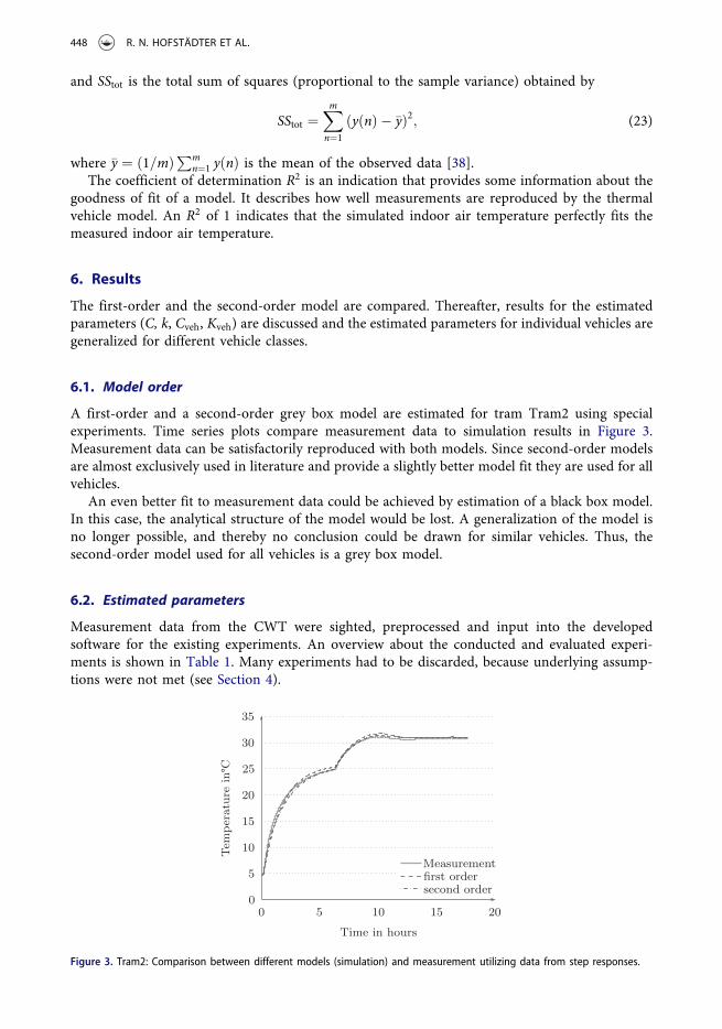
A first-order and a second-order grey box model are estimated for tram Tram2 using specialexperiments. Time series plots compare measurement data to simulation results in Figure 3.Measurement data can be satisfactorily reproduced with both models. Since second-order modelsare almost exclusively used in literature and provide a slightly better model fit they are used for allvehicles.

An even better fit to measurement data could be achieved by estimation of a black box model.In this case, the analytical structure of the model would be lost. A generalization of the model isno longer possible, and thereby no conclusion could be drawn for similar vehicles. Thus, thesecond-order model used for all vehicles is a grey box model.

6.2. Estimated parameters

Measurement data from the CWT were sighted, preprocessed and input into the developedsoftware for the existing experiments. An overview about the conducted and evaluated experi-ments is shown in Table 1. Many experiments had to be discarded, because underlying assump-tions were not met (see Section 4).

Time in hours

0 5 10 15 200

5

10

15

20

25

30

35

Measurementfirst ordersecond order

Figure 3. Tram2: Comparison between different models (simulation) and measurement utilizing data from step responses.

448 R. N. HOFSTÄDTER ET AL.

A summary of average values for all estimated parameters of all identified vehicles can befound in Table 2.

With the estimated parameters the simulation model was established. A comparison betweensimulation and measurement of the indoor air temperature is shown for two metros in Figure 4.Parameters for a model with small deviations could be estimated for all vehicles, as it can be seenin both examples. The deviation between measurement and simulation is similarly small as forTram2, but the considered temperature range is smaller.

6.3. Generalized parameters

In addition to absolute results, the specific heat capacity cveh of the vehicle body is calculated by

cveh ¼ Cveh

mveh; (24)

where mveh is the mass of the vehicle. Results are grouped by vehicle type and plotted in Figure 5(a). The vehicle type is used, because features of a vehicle correlate usually well with the vehicletype. Hence, it is assumed that various features of the vehicle, like number of seats, type of seats(with fabric cover or plastic only) and interior decoration can be mapped into the vehicle class.For example, metros and trams are mostly equipped with seats made of plastic, while main-linevehicles have more comfortable seats with fabric cover. For the two classes tram and main-line, nofurther conclusion is possible, due to the limited data set. In Figure 5(a), it can be seen that the

Time in hours

0 5 10 15 2022

23

24

25

26

27

28

29

30

MeasurementSimulation

(a) Metro1

Time in hours

0 5 10 1518

20

22

24

26

28

30

32

MeasurementSimulation

(b) Metro5

Figure 4. Comparison between estimated models (simulation) and measurements for indoor air temperature utilizing datafrom standard commissioning.

cveh in J/(kg K)

Tram

Metro

Regional

Main-line �

�

�

�

(a) Specific heat capacity of the vehicle body cveh

versus vehicle class

δ in 10 100 200 300 400 500 600 700 800 0 1 2 3 4 5 6 7 8 9 10

Tram

Metro

Regional

Main-line �

�

�

�

(b) Ratio of the two heat capacities δ versus vehicleclass

Figure 5. Boxplots of generalized parameters for each vehicle class.

MATHEMATICAL AND COMPUTER MODELLING OF DYNAMICAL SYSTEMS 449

two classes of metros and regional trains differ considerably from each other. The mean value ofthe specific heat capacity for metros is 372 J/(kg K) and for regional trains, it is 603 J/(kg K). Dueto the small numbers of measurements and the high variance inside the vehicle classes, it cannotbe statistically proven that the difference is significant.

Another generalized result is the ratio δ of the two heat capacities and can be calculated by

δ ¼ Cveh

C: (25)

Figure 5(b) shows the ratio for different vehicle classes. The corresponding numbers are listedin Table 3. It can be clearly seen that the ratio increases from tram through metro and regional tomain-line. Just as it would be expected, since main-line vehicles are a lot heavier than trams andmetros. Hence, their vehicle body has a larger heat capacity.

6.4. Plausibility check

Due to the fact that only a small amount of data are available, a cross validation of models is notpossible. Instead a plausibility check of results is done. There is a maximum of one usableexperiment for each vehicle and this experiment is used for the parameter estimation. InTable 2 and Figure 5(a), it can be observed that the values for the specific heat capacity for thevehicle cveh are in the range from 175 J/(kg K) to 703 J/(kg K). Values are exactly in the expectedrange.

During the construction of the vehicle especially steel (c � 477 J=ðkgKÞ) and aluminium(c � 896 J=ðkgKÞ) are used in larger quantities.

7. Conclusion

This paper presents the estimation of heat capacities and heat transfer coefficients for twodynamic thermal rail vehicle models. Different sources of measurement data are used. Whilespecial experiments are designed for the estimation, some existing measurements can sometimesbe used additionally and comparable results are obtained. Simulation results are in good agree-ment with measurement data, if underlying model assumptions are met. Parameters for allrelevant passenger rail vehicles classes are given: Tram, Metro, Regional and Main-line. Also, itis indicated that grouping into these vehicle classes is justified. The plausibility check shows thatobtained results are generally in the expected range and correlate with the vehicle construction.The estimation results and the generalized parameters provide a first step towards a basis forfuture thermal vehicle models for all relevant rail vehicle classes.

Table 3. Generalized parameters for existing vehicles.

Name cvehJ/(kg K) δ(1)

Tram1 270 0.56Tram2 333 0.55Metro1 533 2.05Metro2 304 1.04Metro3 175 0.71Metro4 487 2.89Metro5 360 2.05Regio1 664 0.11Regio2 577 4.88Regio3 595 3.1Regio4 703 2.88Main1 562 5.47Main2 433 9.35

450 R. N. HOFSTÄDTER ET AL.

This provides a basis for a wide application in the industry: The rail vehicle manufacturer canfall back on the proposed parameters for the dynamic energy consumption calculation (which isalready done in some cases), until those parameters have been measured in the CWT. Calculationsare easier to understand for the customers and operators of rail vehicles, if consistent parametersare used as standard for the thermal vehicle model. By the use of the proposed parameters,numerical values for the dynamic thermal vehicle models are available during the design phase ofthe HVAC to the manufacturer. In addition, the proposed dynamic thermal vehicle models arethe basis for further optimization of all thermal vehicle components. Thus, a modern controller(i.e. a model-based predictive controller) can be designed that uses the proposed models forenergy consumption optimization. The designer is supported by the use of the proposed para-meters, because a laborious analytical calculation is not required.

Measurement of heat capacity and heat transfer on all future vehicles would be greatlybeneficial.

Acknowledgements

The authors thank the three anonymous reviewers whose comments and suggestions helped to improve and clarifythis manuscript.

Disclosure statement

No potential conflict of interest was reported by the authors.

Funding

This work was supported by the project EcoTram: (FFG - Austrian research funding association, [Grant Number:825443]) in cooperation with Schieneninfrastruktur-Dienstleistungsgesellschaft m.b.H, Siemens AG Österreich,Vossloh Kiepe Ges.m.b.H, and Wiener Linien GmbH & Co KG.

References

[1] T. Berger and W. Böck, Radverkehrserhebung Wien – Entwicklungen, Merkmale und Potenziale (2010).Available at http://www.wien.gv.at/stadtentwicklung/studien/pdf/b008167.pdf.

[2] Wiener Linien GmbH and Co KG, 2014 – facts and figures, Vienna, 2014. Available at https://www.wienerlinien.at/media/files/2015/facts_and_figures_2014_151139.pdf.

[3] European Comission, A Sustainable Future for Transport – Towards an Integrated, Technology- Led andUser-Friendly System, 2009, pp. 26. Available at http://ec.europa.eu/transport/strategies/2009_future_of_transport_en.htm.

[4] M. Rosenberger, B. Akagündüz-Binder, K. Conrad, M. Falter, R. Hauswirth, B. Hetzmannseder, J. Hutter, M.Liebhart, K. Mittringer, M. Kirsten, B. Rauscher, and K. Söpper, STEP 2025 – Urban development PlanVienna, Vienna City Administration, Municipal Department 18 (MA 18) – Urban Development andPlanning, 2014, pp. 145. Available at https://www.wien.gv.at/stadtentwicklung/studien/pdf/b008379b.pdf.

[5] W. Struckl, Green Line – Umweltgerechte Produktentwicklungsstrategien für Schienen- fahrzeuge auf Basis derLebenszyklusanalyse des Metrofahrzeuges Oslo, Ph.D. diss., Vienna University of Technology, 2007.

[6] C. Isenschmid, S. Menth, and P. Oelhafen, Energieverbrauch und Einsparpotential des S-Bahn-GliederzugsRABe 525 “Nina” der BLS AG, Eisenbahn-Revue 8–9 (2013), pp. 398–403.

[7] J. Powell, A. González-Gil, and R. Palacin, Experimental assessment of the energy consumption of urban railvehicles during stabling hours: Influence of ambient temperature, Appl. Therm. Eng. 66 (2014), pp. 541–547.doi:10.1016/j.applthermaleng.2014.02.057

[8] G. Richter, Ecotram research project: How much energy is used by the HVAC of a tram? Measurements in theclimatic wind tunnel and in service, Railvolution 10 (2010).

[9] H. Amri, R.N. Hofstädter, and M. Kozek, Energy efficient design and simulation of a demand controlledheating and ventilation unit in a metro vehicle, IEEE Forum on Integrated and Sustainable TransportationSystem (FISTS), Vienna, June 2011, pp. 7–12.

MATHEMATICAL AND COMPUTER MODELLING OF DYNAMICAL SYSTEMS 451

[10] B. Beusen, B. Degraeuwe, and P. Debeuf, Energy savings in light rail through the optimization of heating andventilation, Transport. Res. D Trans. Environ. 23 (2013), pp. 50–54. doi:10.1016/j.trd.2013.03.005

[11] J.S. Brown and P.A. Domanski, Review of alternative cooling technologies, Appl. Therm. Eng. 64 (2014), pp.252–262. doi:10.1016/j.applthermaleng.2013.12.014

[12] Z. Zhang, S. Liu, and L. Tian, Thermodynamic analysis of air cycle refrigeration system for chinese train airconditioning, Syst. Eng. Proc. 1 (2011), pp. 16–22. Engineering and Risk Management. doi:10.1016/j.sepro.2011.08.004

[13] A. Afram and F. Janabi-Sharifi, Review of modeling methods for HVAC systems, Appl. Therm. Eng. 67 (2014),pp. 507–519. doi:10.1016/j.applthermaleng.2014.03.055

[14] D. Marcos, F.J. Pino, C. Bordons, and J.J. Guerra, The development and validation of a thermal model for thecabin of a vehicle, Appl. Therm. Eng. 66 (2014), pp. 646–656. doi:10.1016/j.applthermaleng.2014.02.054

[15] B. Torregrosa-Jaime, F. Bjurling, J.M. Corberán, F. Di Sciullo, and J. Payá, Transient thermal model of avehicle’s cabin validated under variable ambient conditions, Appl. Therm. Eng. 75 (2014), pp. 45–53.

[16] J. Marachlian, R. Benelmir, A.E. Bakkali, and G. Olivier, Exergy based simulation model for vehicle HVACoperation, Appl. Therm. Eng. 31 (2011), pp. 696–700. doi:10.1016/j.applthermaleng.2010.10.001.

[17] MAGNA, Kuli: Thermal management simulation software (2014). Available at http://www.kuli.at.[18] J. Rugh, K. Bennion, A. Brooker, J. Langewisch, K. Smith, and J. Meyer, PHEV/EV integrated vehicle thermal

management – development of a KULI model to assess combined cooling loops, in Vehicle ThermalManagement Systems Conference and Exhibition (VTMS10), I.o.M.E. (IMechE), ed., Woodhead Publishing,2011, pp. 649–660, Available at http://www.sciencedirect.com/science/article/pii/B9780857091727500567.

[19] F. Felgner, R. Merz, and L. Litz, Modular modelling of thermal building behaviour using modelica, Math.Comput. Model. Dynam. Syst. 12 (2006), pp. 35–49. doi:10.1080/13873950500071173

[20] W. Liu, Q. Deng, W. Huang, and R. Liu, Variation in cooling load of a moving air- conditioned traincompartment under the effects of ambient conditions and body thermal storage, Appl. Therm. Eng. 31 (2011),pp. 1150–1162. doi:10.1016/j.applthermaleng.2010.12.010

[21] R.N. HofstäDter and M. Kozek, Holistic thermal simulation model of a tram, Conference on ComputerModelling and Simulation, Proceedings, Brno, Czech Republic, 2011.

[22] W. Li and J. Sun, Numerical simulation and analysis of transport air conditioning system integrated withpassenger compartment, Appl. Therm. Eng. 50 (2013), pp. 37–45. doi:10.1016/j.applthermaleng.2012.05.030

[23] G. Haller, Der neue Klima-Wind-Kanal in Wien, in Zevrail Glasers Annalen 126, 38. GrazerSchienenfahrzeugtagung, Institute of Railway Engineering and Transport Economy, Graz University ofTechnology, Deutsche Maschinentechnische Gesellschaft (DMG), Berlin, 2002, pp. 22–27.

[24] DIN EN 13129-2:2004-10, Railway Applications – Air Conditioning for Main Line Rolling Stock – Part 2: TypeTests, Beuth, Berlin, 2004. German Version.

[25] DIN EN 14750-2:2006-08, Railway Applications - Air Conditioning for Urban and Suburban Rolling Stock -Part 2: Type Tests, Beuth, Berlin, 2006. German Version.

[26] G. Haller, The benefits of climatic testing of rail vehicles, Foreign Roll. Stock 3 (2009), pp. 11.[27] K.H. Grote and J. Feldhusen, Dubbel – Taschenbuch für den Maschinenbau, 23rd ed., Springer, Berlin/

Heidelberg, 2011.[28] DIN V 18599, Energy Efficiency of Buildings – Calculation of the net, Final and Primary Energy Demand for

Heating, Cooling, Ventilation, Domestic Hot Water and Lighting, Beuth, Berlin, 2011. Prestandard, GermanVersion.

[29] European Parliament and the Council, Directive 2010/31/EU of the European Parliament and of the Councilof 19 May 2010 on the Energy Performance of Buildings (recast), 2010.

[30] Verordnung zur Änderung der Energieeinsparverordnung, Bundesgesetzblatt Jahrgang 2013 Teil I Nr. 67,Bundesanzeiger Verlag, Köln, 2013, pp. 3951–3990.

[31] C. Dullinger, W. Struckl, and M. Kozek, A modular thermal simulation tool for computing energy consump-tion of hvac units in rail vehicles, Appl. Therm. Eng. 78 (2015), pp. 616–629. doi:10.1016/j.applthermaleng.2014.11.065

[32] C.M. Close and D.K. Frederick, Modeling and Analysis of Dynamic Systems, 2nd ed., John Wiley & Sons,Hoboken, 1994.

[33] L. Ljung, System Identification: Theory for the User, Pearson Education, Upper Saddle River, NJ, 1998.[34] L. Ljung, Prediction error estimation methods, Circuits Syst. Signal Process. 21 (2002), pp. 11–21. doi:10.1007/

BF01211648[35] K. Ogata, Discrete-Time Control Systems, 2nd ed., Prentice Hall, Upper Saddle River, NJ, 1995, p. 1.[36] Y. Koubaa, Application of least-squares techniques for induction motor parameters estimation, Math. Comput.

Model. Dynam. Syst. 12 (2006), pp. 363–375. doi:10.1080/13873950500064103[37] MATLAB, Version 7.10.0 (R2010a), The MathWorks, Natick, MA, 2010.[38] B. Everitt, Cambridge Dictionary of Statistics, Cambridge University Press, Cambridge, 1998.

452 R. N. HOFSTÄDTER ET AL.