Heat, Ocean, and Atmosphere

Origins of the Warming ’hiatus’ Concept

Jan GalkowskiWestwood Statistical Studiosempirical bayesian@ieee.org

Westwood, MA 02090

April 26, 2014(revised draft 001)

Heat, Ocean, and Atmosphere: A summary April 26, 2014, revised draft 001

When present, changes are indicated with red changebars, such as to the left of this paragraph.

Westwood Statistical Studios Page 1

Heat, Ocean, and Atmosphere: A summary April 26, 2014, revised draft 001

1 How Heat Flows and Why It Matters

Heat is most often experienced as energy density, related to temperature. While technically temperatureis only meaningful for a body in thermal equilibrium, temperature is the operational definition of heatcontent, both in daily life and as a scientific measurement, whether at a point or averaged. For the presentdiscussion, it is taken as given that increasing atmospheric concentrations of carbon dioxide trap andre-radiate Earth blackbody radiation to its surface, resulting in a higher mean blackbody equilibrationtemperature for the planet, via radiative forcing [1, 2, 3, 4]. The question is, how does a given Jouleof energy travel? Once entrained on Earth, does it remain in atmosphere? Warm the surface? Go intothe oceans? And, especially, if it does go into the oceans, what is its residence time before released toatmosphere? These are important questions [5, 6]. Because of the miscibility of energy, questions ofresidence time are very difficult to answer. A Joule of energy can’t be tagged with a radioisotope likematter sometimes can. In practice, energy content is estimated as a constant plus the time integral ofenergy flux across a well-defined boundary using a baseline moment.

Variability is a key aspect of natural systems, whether biological or large scale geophysical systems suchas Earth’s climate [7]. Variability is also a feature of statistical models used to describe behavior of naturalsystems, whether they be straightforward empirical models or models based upon ab initio physicalcalculations. Some of the variability in models captures the variability of the natural systems which theydescribe, but some variability is inherent in the mechanism of the models, an artificial variability whichis not present in the phenomena they describe. (The nomenclature can be confusing. With respect toobservations, variability arising due to choice of method is sometimes called structural uncertainty [37,38].) No doubt, there is always some variability in natural phenomena which no model captures. Thisvariability can be partitioned into parts, at the risk of specifying components which are not directlyobservable. Sometimes they can be inferred.

Models of planetary climate are both surprisingly robust and understood well enough that appreciablesimplifications are possible, such as setting aside fluid dynamism, without damaging their utility [2, Pref-ace]. Thus, long term or asymptotic and global predictions of what consequences arise when atmosphericcarbon dioxide concentrations double or triple are known pretty well. What is less certain are the dis-sipation and diffusion mechanisms for this excess energy and its behavior in time [8, 9, 10, 11]. Thereis keen interest in these mechanisms because of the implications differing magnitudes have for regionalclimate forecasts and economies [12,13,14]. Moreover, there is a natural desire to obtain empirical con-firmation of physical calculations, as difficult as that might be, and as subjective as judgments regardingquality of predictions might be [15, 16, 17, 18, 19, 20, 21, 22, 23, 24, 25, 36, 37, 26, 27, 28, 29, 30, 31].

Observed rates of surface temperatures in recent decades have shown a moderating slope compared withboth long term statistical trends and climate model projections [32, 33, 15, 34, 36, 18, 21, 35, 16]. It’s thepurpose of this article to present this evidence, and report the research literature’s consensus on where theheat resulting from radiative forcing is going, as well as sketch some implications of that containment.Westwood Statistical Studios Page 2

Heat, Ocean, and Atmosphere: A summary April 26, 2014, revised draft 001

2 On Surface Temperatures, Land and Ocean

Independently of climate change, monitoring surface temperatures globally is a useful geophysical project.They are accessible, can be measured in a number of ways, permitting calibration and cross-checking,

are taken at convenient boundaries, land-and-atmosphere or ocean-and-atmosphere, and coincide withthe living space about which we most care. Nevertheless, like any large observational effort in the field,such measurements need careful assessment and processing before they can be properly interpreted. TheBerkeley Earth Surface Temperature (“BEST”) Project represents the most comprehensive such effort,but it was not possible without many predecessors, such as HadCRUT4, and works by Kennedy, et al andRohde [39, 37, 27, 40, 41].

Surface temperature is a manifestation of four interacting processes. First, there is warming of the surfaceby the atmosphere. Second, there is lateral heating by atmospheric convection and latent heat in watervapor. Third, during daytime, there is warming of the surface by the Sun or insolation which survivesreflection. Last, there is warming of the surface from below, either latent heat stored subsurface, orgeologic processes. Roughly speaking, these are ordered from most important to least. These are allmanifestations of energy flows, a consequence of equalization of different contributions of energy toEarth.

Physically speaking, the total energy of the Earth climate system is a constant plus the time integralof energy of non-reflected insolation less the energy of the long wave radiation or blackbody radiationwhich passes from Earth out to space, plus geothermal energy ultimately due to radioisotope decay withinEarth’s aesthenosphere and mantle, plus thermal energy generated by solid Earth and ocean tides, pluswaste heat from anthropogenic combustion and power sources. (There are tiny amounts of heating dueto impinging ionizing radiation from space, and changes in Earth’s magnetic field.) The amount of non-reflected insolation depends upon albedo, which itself slowly varies. The amount of long wave radiationleaving Earth for space depends upon the amount of water aloft, by amounts and types of greenhousegases, and other factors. Our understanding of this has improved rapidly, as can be seen by contrastingKiehl, et al in 1997 with Trenberth, et al in 2009 and the IPCC’s 2013 WG1 Report [42, 43, 44]. SteveEasterbrook has given a nice summary of radiative forcing at his blog, as well as provided a succinctrecap of the 2013 IPCC WG1 Report and its take on energy flows elsewhere at the Azimuth blog. I referthe reader to those references for information about energy budgets, what we know about them, and whatwe do not.

Some ask whether or not there is a physical science basis for the “moderation” in global surface tempera-tures and, if there is, how that might work. It is an interesting question, for such a conclusion is predicatedupon observed temperature series being calibrated and used correctly, and, further, upon insufficient pre-cision in climate model predictions, whether simply perceived or actual. Hypothetically, it could be thatthe temperature models are not being used correctly and the models are correct, and which evidence wechoose to believe depends upon our short-term goals. Surely, from a scientific perspective, what’s wantedWestwood Statistical Studios Page 3

Heat, Ocean, and Atmosphere: A summary April 26, 2014, revised draft 001

is a reconciliation of both, and that is where many climate scientists invest their efforts. This is also aninteresting question because it is, at its root, a statistical one, namely, how do we know which model isbetter [46, 7, 25, 45, 47, 48, 49]?

A first graph, Figure 1.1, depicting evidence of warming is, to me, quite remarkable. A similar graph

Figure 1.1: Ocean temperatures at depth, from http://www.yaleclimatemediaforum.org/2013/09/

examining-the-recent-slow-down-in-global-warming/.

is shown in the important series recapping the recent IPCC Report by Steve Easterbrook [50]. A greatdeal excess heat is going into the oceans. In fact, most of it is. This can happen in many ways, but onedramatic way is due to a phase of the El Nino Southern Oscillation (“ENSO”).

The trade winds along the Pacific equatorial region vary in strength. When they are weak, the phe-nomenon called El Nino is seen, affecting weather in the United States and in Asia. Evidence for ElWestwood Statistical Studios Page 4

Heat, Ocean, and Atmosphere: A summary April 26, 2014, revised draft 001

Figure 1.2: Oblique view of variability of Pacific equatorial region from El Nino to La Nina and back. Vertical heigh of ocean is exaggeratedto show piling up of waters in the Pacific warm pool. (Note that this will be replaced on the Web page with a GIF file.)

Nino includes elevated sea-surface temperatures (“SSTs”) in the eastern Pacific. This short-term cli-mate variation brings increased rainfall to the southern United States and Peru, and drought to east Asiaand Australia, often triggering large wildfires there. The reverse phenomenon, La Nina, is produced bystrong trades, and results in cold SSTs in the eastern Pacific, and plentiful rainfall in east Asia and north-ern Australia. Strong trades actually pile ocean water up against Asia, and these warmer-than-averagewaters push surface waters there down, creating a cycle of returning cold waters back to the eastern Pa-cific. This process is depicted in Figures 1.2 and 1.3. At its peak, a La Nina causes waters to accumulatein the Pacific warm pool, and this results in surface heat being pushed into the deep ocean. To the degreeto which heat goes into the deep ocean, it is not available in atmosphere. To the degree to which thetrades do not pile waters into the Pacific warm pool and, ultimately, into the depths, that warm water isin contact with atmosphere [51]. There are suggestions warm waters at depth rise to the surface [52].

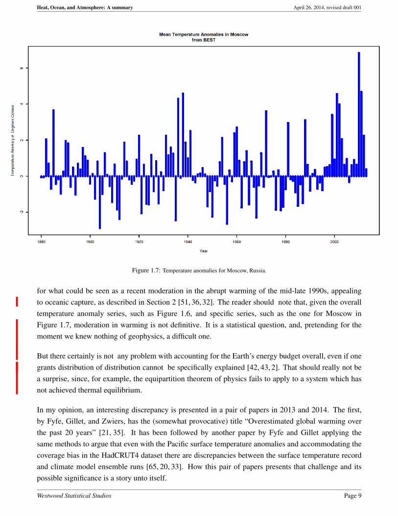
Documentation of land and ocean surface temperatures is done in variety of ways. There are severalimportant sources, including Berkeley Earth, NASA GISS, and the Hadley Centre/Climatic Research Unit(“CRU”) data sets [39, 53, 37]. The three, referenced here as BEST, GISS, and HadCRUT4, respectivelyhave been compared by Rohde [41]. They differ in duration and extent of coverage, but allow comparableinferences. For example, a linear regression establishing a trend using July monthly average temperaturesfrom 1880 to 2012 for Moscow from GISS and BEST agree that Moscow’s July 2010 heat was 3.67Westwood Statistical Studios Page 5

Heat, Ocean, and Atmosphere: A summary April 26, 2014, revised draft 001

Figure 1.3: Trade winds vary in strength, having consequences for pooling and flow of Pacific waters and sea surface temperatures. (Notethat this will be replaced on the Web page with a GIF file.)

Figure 1.4: Strong trade winds cause the warm surface waters of the equatorial Pacific to pile up against Asia.

standard deviations from the long term trend. (3.667 (GISS) versus 3.670 (BEST).) Nevertheless, thereis an important difference between BEST and GISS, on the one hand, and HadCRUT4.

BEST and GISS attempt to capture and convey a single best estimate of temperatures on Earth’s surface,and attach an uncertainty measure to each number. Sometimes, because of absence of measurements orequipment failures, there are no measurements, and these are clearly marked in the series. HadCRUT4 isdifferent. With HadCRUT4 the uncertainty in measurements is described by a hundred member ensembleof values, actually a 2592-by-1967 matrix. Rows correspond to observations from 2592 patches, 36 inlatitude, and 72 in longitude, with which it represents the surface of Earth. Columns correspond to eachmonth from January 1850 to November 2013. It is possible for any one of these cells to be coded as“missing”. This detail is important because HadCRUT4 is the basis for a paper suggesting the pause inglobal warming is structurally inconsistent with climate models. That paper will be discussed later.

Westwood Statistical Studios Page 6

Heat, Ocean, and Atmosphere: A summary April 26, 2014, revised draft 001

Figure 1.5: Global surface temperature anomalies relative to a 1950-1980 baseline.

3 Rumors of Pause

Figure 1.5 shows the global mean surface temperature anomalies relative to a standard baseline, 1950-1980. Before going on, consider that figure. Study it. What can you see in it?

Figure 1.6 shows the same graph, but now with two trendlines obtained by applying a smoothing spline,one smoothing more than another. One of the two indicates an uninterrupted uptrend. The other shows apeak and a downtrend, along with wiggles around the other trendline. Note the smoothing algorithm isthe same in both cases, differing only in the setting of a smoothing parameter1. Which is correct? Whatis “correct”?

Figure 1.1 shows trend curves for ocean heat content over roughly the same period. Figure 1.7 shows atime series of anomalies for Moscow, in Russia. Do these all show the same trends? These are difficultquestions, but the changes seen in Figure 1.6 could be evidence of a warming “hiatus” [54, 32]. (Theterm hiatus has a formal meaning in climate science, as described by the IPCC itself [44, Box TS.3].)Note that, given Figure 1.6 the most which can be said about it is that there is a reduction in the rate of

1Called “SPAR”.

Westwood Statistical Studios Page 7

Heat, Ocean, and Atmosphere: A summary April 26, 2014, revised draft 001

Figure 1.6: Global surface temperature anomalies relative to a 1950-1980 baseline, with two smoothing splines printed atop.

temperature increase. We’ll have a more careful look at this in Section 4. With that said, people havesought reasons and assessments of how important this phenomenon is. The answers have ranged fromthe conclusive “Global warming has stopped” to “Perhaps the slowdown is due to ’natural variability”’,to “Perhaps it’s all due to ’natural variability”’ to “There is no statistically significant change”. Let’s seewhat some of the perspectives are.

It is hard to find a scientific paper which advances the proposal that climate might be or might havebeen cooling in recent history. The earliest I can find are repeated presentations by a single geologistin the proceedings of the Geological Society of America, a conference which, like many, gives paperslimited peer review [55, 55, 56, 57, 58, 59, 60, 61]. It is difficult to comment on this work since their fullmethods are not available for review. The content of the abstracts appear to ignore the possibility oflagged response in any physical system.

These claims were summarized by Easterling and Wehner in 2009, attributing claims of a “pause” tocherry-picking of sections of the temperature time series, such as 1998-2008, and what might be calledmedia amplification [54]. Further, technical inconsistencies within the scientific enterprise, perfectlynormal in its deployment and management of new methods of measurement, have been highlighted andabused to parlay claims of global cooling [62, 63, 64]. Based upon subsequent papers, climate scienceseemed to not only need to explain such variability is to be expected, but to provide a specific explanationWestwood Statistical Studios Page 8

Heat, Ocean, and Atmosphere: A summary April 26, 2014, revised draft 001

Figure 1.7: Temperature anomalies for Moscow, Russia.

for what could be seen as a recent moderation in the abrupt warming of the mid-late 1990s, appealingto oceanic capture, as described in Section 2 [51, 36, 32]. The reader should note that, given the overalltemperature anomaly series, such as Figure 1.6, and specific series, such as the one for Moscow inFigure 1.7, moderation in warming is not definitive. It is a statistical question, and, pretending for themoment we knew nothing of geophysics, a difficult one.

But there certainly is not any problem with accounting for the Earth’s energy budget overall, even if onegrants distribution of distribution cannot be specifically explained [42, 43, 2]. That should really not bea surprise, since, for example, the equipartition theorem of physics fails to apply to a system which hasnot achieved thermal equilibrium.

In my opinion, an interesting discrepancy is presented in a pair of papers in 2013 and 2014. The first,by Fyfe, Gillet, and Zwiers, has the (somewhat provocative) title “Overestimated global warming overthe past 20 years” [21, 35]. It has been followed by another paper by Fyfe and Gillet applying thesame methods to argue that even with the Pacific surface temperature anomalies and accommodating thecoverage bias in the HadCRUT4 dataset there are discrepancies between the surface temperature recordand climate model ensemble runs [65, 20, 33]. How this pair of papers presents that challenge and itspossible significance is a story unto itself.

Westwood Statistical Studios Page 9

Heat, Ocean, and Atmosphere: A summary April 26, 2014, revised draft 001

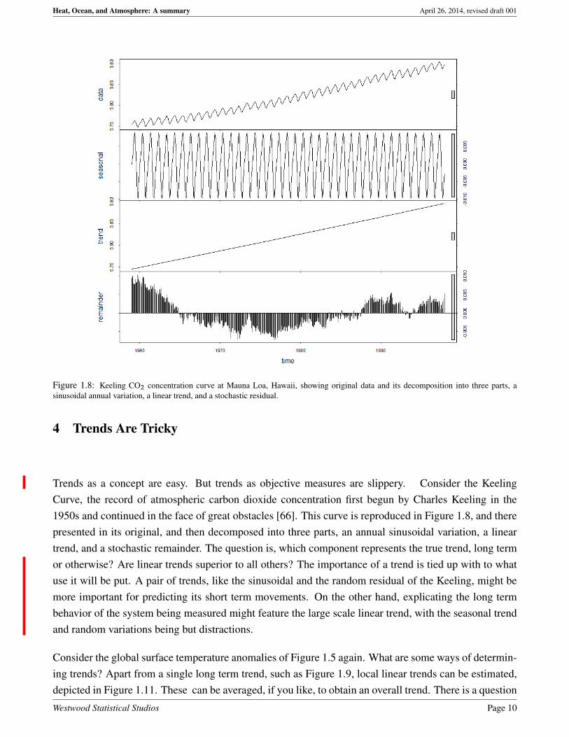
Figure 1.8: Keeling CO2 concentration curve at Mauna Loa, Hawaii, showing original data and its decomposition into three parts, asinusoidal annual variation, a linear trend, and a stochastic residual.

4 Trends Are Tricky

Trends as a concept are easy. But trends as objective measures are slippery. Consider the KeelingCurve, the record of atmospheric carbon dioxide concentration first begun by Charles Keeling in the1950s and continued in the face of great obstacles [66]. This curve is reproduced in Figure 1.8, and therepresented in its original, and then decomposed into three parts, an annual sinusoidal variation, a lineartrend, and a stochastic remainder. The question is, which component represents the true trend, long termor otherwise? Are linear trends superior to all others? The importance of a trend is tied up with to whatuse it will be put. A pair of trends, like the sinusoidal and the random residual of the Keeling, might bemore important for predicting its short term movements. On the other hand, explicating the long termbehavior of the system being measured might feature the large scale linear trend, with the seasonal trendand random variations being but distractions.

Consider the global surface temperature anomalies of Figure 1.5 again. What are some ways of determin-ing trends? Apart from a single long term trend, such as Figure 1.9, local linear trends can be estimated,depicted in Figure 1.11. These can be averaged, if you like, to obtain an overall trend. There is a question

Westwood Statistical Studios Page 10

Heat, Ocean, and Atmosphere: A summary April 26, 2014, revised draft 001

Figure 1.9: Global surface temperature anomalies relative to a 1950-1980 baseline, with long term linear trend atop.

of what to do if local intervals for fitting the little lines overlap, since these are not independent of oneanother. There are a number of statistical devices for making them independent. One way is to do cleverkinds of random sampling from a population of linear trends. Another way is to shrink the intervals untilthey are infinitesimally small, and, so, necessarily independent. That’s just the point slope of a curvegoing through the data, or its first derivative. Numerical methods exist of estimating these, one involvinga smoothing spline and estimating the derivative(s) of that [67]. Such an estimate is shown in Figure 1.12where the instantaneous slope is plotted atop the data of Figure 1.5. The spline is a cubic spline andthe smoothing parameter is determined by generalized cross-validation [68]. (The smoothing parametersspecifies the weight of the penalty term for the second derivative of curvature.)

What else might we do? We could go after a really good approximation to the data of Figure 1.5. Onepossibility is to use the Bayesian Rauch-Tung-Striebel (“RTS”) smoother to get a good approximation forthe underlying curve and estimate the derivatives of that [69]. There is a problem in that the prior vari-ances of the signal need to be estimated. The larger the ratio of the estimate of the observations varianceto the estimate of the process variance is, the smoother the RTS solution. (Here, the process variance wastaken here to be 1

300of the observations variance.) The RTS smoother result for two variance values of

0.156 and high 0.0.312 is shown in Figure 1.13. These are 4 and 8 times the decorrelated variance valuefor the series of 0.039, estimated separately.

Westwood Statistical Studios Page 11

Heat, Ocean, and Atmosphere: A summary April 26, 2014, revised draft 001

Figure 1.10: Global surface temperature anomalies relative to a 1950-1980 baseline, with randomly placed trends from local linear having5 year support atop.

Combining all six methods of estimating trends results in Figure 1.14 which shows the overprinteddensities of slopes. To match each of the methods by statistical weight, since, for instance, the spline andRTS methods produce many more estimates of trends than do the local linear fits, 30 randomly selectedtrends were chosen from each of the kinds of trends, and these are plotted. Note the spread of possibilitiesgiven by the local linear fits. Such fits to HadCRUT4 time series were used by Fyfe, Gillet, and Zwiersin their 2013 paper [21, 35].

Westwood Statistical Studios Page 12

Heat, Ocean, and Atmosphere: A summary April 26, 2014, revised draft 001

Figure 1.11: Global surface temperature anomalies relative to a 1950-1980 baseline, with randomly placed trends from local linear having10 year support atop.

Westwood Statistical Studios Page 13

Heat, Ocean, and Atmosphere: A summary April 26, 2014, revised draft 001

Figure 1.12: Global surface temperature anomalies relative to a 1950-1980 baseline, with instaneous numerical estimates of derivativesatop. Support for the smoothing spline used to calculate the derivatives is obtained using generalized cross validation [67]. Note how thevalue of the first derivative never drops below zero although its magnitude decreases as time approaches 2012.

Westwood Statistical Studios Page 14

Heat, Ocean, and Atmosphere: A summary April 26, 2014, revised draft 001

Figure 1.13: Global surface temperature anomalies relative to a 1950-1980 baseline, with fits using the Rauch-Tung-Striebel smootherplaced atop, in magenta and dark red. The former uses a prior variance of 4 times that of the Figure 1.5 data corrected for serial correlation.The latter uses a prior variance of 4 times that. The instaneous numerical estimates derived from the two solutions are shown in green andblue, respectively. Note the two solutions are essentially identical.

Westwood Statistical Studios Page 15

Heat, Ocean, and Atmosphere: A summary April 26, 2014, revised draft 001

Figure 1.14: Composite of trends estimated using the long term linear fit (the vertical black line), the local linear fits with 5 years separation(navy blue trace), the local linear fits with 10 years separation (dashed navy blue trace), the smoothing spline (blue trace), the RTS smootherwith variance 4 times the corrected estimate for the data as the prior variance (green trace), and the RTS smoother with eight times thecorrected estimate for the data (red trace). 30 randomly chosen (without replacement) trends have densities estimated to construct this chart.

Westwood Statistical Studios Page 16

Heat, Ocean, and Atmosphere: A summary April 26, 2014, revised draft 001

5 Internal Decadal Variability

The recent IPCC AR5 WG1 Report sets out the context [44, Box TS.3]:

Hiatus periods of 10 to 15 years can arise as a manifestation of internal decadal climate vari-ability, which sometimes enhances and sometimes counteracts the long-term externally forcedtrend. Internal variability thus diminishes the relevance of trends over periods as short as 10to 15 years for long-term climate change (Box 2.2, Section 2.4.3). Furthermore, the timingof internal decadal climate variability is not expected to be matched by the CMIP5 histori-cal simulations, owing to the predictability horizon of at most 10 to 20 years (Section 11.2.2;CMIP5 historical simulations are typically started around nominally 1850 from a control run).However, climate models exhibit individual decades of GMST trend hiatus even during a pro-longed phase of energy uptake of the climate system (e.g., Figure 9.8; Easterling and Wehner,2009; Knight et al., 2009), in which case the energy budget would be balanced by increasingsubsurface-ocean heat uptake (Meehl et al., 2011, 2013a; Guemas et al., 2013).

Owing to sampling limitations, it is uncertain whether an increase in the rate of subsurface-ocean heat uptake occurred during the past 15 years (Section 3.2.4). However, it is very likely2

that the climate system, including the ocean below 700 m depth, has continued to accumu-late energy over the period 1998-2010 (Section 3.2.4, Box 3.1). Consistent with this energyaccumulation, global mean sea level has continued to rise during 1998-2012, at a rate onlyslightly and insignificantly lower than during 1993-2012 (Section 3.7). The consistency be-tween observed heat-content and sea level changes yields high confidence in the assessmentof continued ocean energy accumulation, which is in turn consistent with the positive radia-tive imbalance of the climate system (Section 8.5.1; Section 13.3, Box 13.1). By contrast,there is limited evidence that the hiatus in GMST trend has been accompanied by a slowerrate of increase in ocean heat content over the depth range 0 to 700 m, when comparing theperiod 2003-2010 against 1971-2010. There is low agreement on this slowdown, since threeof five analyses show a slowdown in the rate of increase while the other two show the increasecontinuing unabated (Section 3.2.3, Figure 3.2).

During the 15-year period beginning in 1998, the ensemble of HadCRUT4 GMST trends liesbelow almost all model-simulated trends (Box 9.2 Figure 1a), whereas during the 15-yearperiod ending in 1998, it lies above 93 out of 114 modelled trends (Box 9.2 Figure 1b; Had-CRUT4 ensemble-mean trend 0:26 ıC per decade, CMIP5 ensemble-mean trend 0:16 ıC perdecade). Over the 62-year period 1951-2012, observed and CMIP5 ensemble-mean trendsagree to within 0:02 ıC per decade (Box 9.2 Figure 1c; CMIP5 ensemble-mean trend 0:13 ıCper decade). There is hence very high confidence that the CMIP5 models show long-term

2“In this Report, the following terms have been used to indicate the assessed likelihood of an outcome or a result: Virtually certain 99�100% probability,Very likely 90�100%, Likely 66�100%, About as likely as not 33�66%, Unlikely 0-33%, Very unlikely 0-10%, Exceptionally unlikely 0-1%. Additionalterms (Extremely likely: 95 � 100%, More likely than not > 50 � 100%, and Extremely unlikely 0-5%) may also be used when appropriate. Assessedlikelihood is typeset in italics, e.g., very likely (see Section 1.4 and Box TS.1 for more details).”

Westwood Statistical Studios Page 17

Heat, Ocean, and Atmosphere: A summary April 26, 2014, revised draft 001

GMST trends consistent with observations, despite the disagreement over the most recent 15-year period. Due to internal climate variability, in any given 15-year period the observedGMST trend sometimes lies near one end of a model ensemble (Box 9.2, Figure 1a, b; East-erling and Wehner, 2009), an effect that is pronounced in Box 9.2, Figure 1a, because GMSTwas influenced by a very strong El Nino event in 1998.

The contributions of Fyfe, Gillet, and Zwiers (“FGZ”) are to (a) pin down this behavior for a 20 yearperiod using the HadCRUT4 data, and, to my mind, more importantly, (b) to develop techniques forevaluating runs of ensembles of climate models like the CMIP5 suite without commissioning specfic runsfor the purpose [21,33]. This, if it were to prove out, would be an important experimental advance, sinceclimate models demand expensive and extensive hardware, and the number of people who know how toprogram and run them is very limited, possibly a more limiting practical constraint than the hardware [70].(“”It’s great there’s a new initiative,” says modeler Inez Fung of DOE’s Lawrence Berkeley NationalLaboratory and the University of California, Berkeley. ”But all the modeling efforts are very short-handed. More brains working on one set of code would be better than working separately”” [70].) FGZtry to explicitly model trends due to internal variability [35]. They begin with two equations:

Mij .t/ D um.t/ C Eintij .t/ C Emodi.t/; i D 1; : : : ; N m; j D 1; : : : ; Ni(1.1)

Ok.t/ D uo.t/ C Einto.t/ C Esampk.t/; k D 1; : : : ; N o(1.2)

with time explicitly indicated, unlike FGZ [35, page 2]. i is the model membership index. j is the indexof the i th model’s j th ensemble. Here, Mij .t/ and Ok.t/ are trends calculated using models or obser-vations, respectively. um.t/ and uo.t/ denote the “true, unknown, deterministic trends due to externalforcing” common to models and observations, respectively [35]. Eintij .t/ and Einto.t/ are the perturba-tions to trends due to internal variability of models and observations. Emodi.t/ denotes error in climatemodel trends for model i . Esampk.t/ denotes the sampling error in the kth sample. Notably FGZ assumeEmodi.t/ are exchangeable with each other as well, at least for the same time t . Note that while the in-ternal variability of climate models Eintij .t/ varies from model-to-model, run-to-run, and time-to-time,the ‘internal variability of observations’, namely Einto.t/, is assumed to only vary with time.

The technical innovation FGZ use is to employ bootstrap resampling on the observations ensemble ofHadCRUT4 and an ensemble of runs of 38 CMIP5 climate models to perform what is essentially a two-sample comparison [71,72]. In doing so, they explicitly assume, in the framework above, exchangeabilityof models. (Exchangeability is a weaker assumption than independence. Random variables are exchange-able if their joint distribution only depends upon the set of variables, and not their order [73,74,75]. Notethe caution in Coolen [76].) k runs over the bootstrap samples taken from HadCRUT4 observations.

So, what is a bootstrap? In its simplest form, a bootstrap is a nonparametric, often robust, frequentisttechnique for sampling the distribution of a function of a set of population parameters, generally irre-spective of the nature or complexity of that function, or the number of parameters. Since estimates of thevariance of that function are themselves functions of population parameters, assuming the variance ex-ists, the bootstrap can also be used to estimate the precision of the first set of samples, where “precision”Westwood Statistical Studios Page 18

Heat, Ocean, and Atmosphere: A summary April 26, 2014, revised draft 001

is the reciprocal of variance. In the case in question here, with FGZ, the bootstrap is being used to deter-mine if the distribution of surface temperature trends as calculated from observations and the distributionof surface temperature trends as calculated from climate models for the same period have in fact similarmeans. This is done by examining differences of paired trends, one coming from an observation sample,one coming from a model sample, and assessing the degree of discrepancy based upon the variances ofthe observations trends distribution and of the models trends distribution.

The equations (1.1) and (1.2) can be re-written:

Mij .t/ � Eintij .t/ D um.t/ C Emodi.t/; i D 1; : : : ; N m; j D 1; : : : ; Ni(1.3)

Ok.t/ � Einto.t/ D uo.t/ C Esampk.t/; k D 1; : : : ; N o(1.4)

moving the trends in internal variability to the left, calculated side. Both Eintij .t/ and Einto.t/ are notdirectly observable. Without some additional assumptions, which are not explicitly given in the FGZpaper, such as

Eintij .t/ � N .0; †model int/(1.5)

Einto.t/ � N .0; †obs int/(1.6)

we can’t really be sure we’re seeing Ok.t/ or Ok.t/�Einto.t/, or at least Ok.t/ less the mean of Einto.t/.The same applies to Mij .t/ and Eintij .t/. Here †model int and †obs int are covariances among models andamong observations. FGZ essentially say these are diagonal with their statement “An implicit assump-tion is that sampling uncertainty in [observation trends] is independent of uncertainty due to internalvariability and also independent of uncertainty in [model trends]” [35]. They might not be so, but it isreasonable to suppose their diagonals are strong, and that there is a row-column exchange operator onthese covariances which can produce banded matrices.

Westwood Statistical Studios Page 19

Heat, Ocean, and Atmosphere: A summary April 26, 2014, revised draft 001

6 On Reconciliation

The centerpiece of the FGZ result is their Figure 1, reproduced here as Figure 1.15. Their conclusion, thatclimate models do not properly capture surface temperature observations for the given periods, is basedupon the significant separate of the red density from the grey density, even measuring that separationusing pooled variances. But, surely, a remarkable feature of these graphs is not only the separation of themeans of the two densities, but the marked difference between the variance of the two densities. Whyare climate models so less precise than HadCRUT4 observations? Conceivably, why do climate models

Figure 1.15: Figure 1 from Fyfe, Gillet, Zwiers [21].

not agree with one another so dramatically? We cannot tell without getting into CMIP5 details, but thesame result could be obtained if the climate models came in three Gaussian populations, each with avariance 1.5x that of the observations, but mixed together. We could also obtain the same result if, forsome reason, the variance of the HadCRUT4 was markedly understated.

That brings us back to the comments about HadCRUT4 made at the end of Section 2. HadCRUT4 isnoted for “drop outs” in observations, where either the quality of an observation on a patch of Earth waspoor or the observation was missing altogether for a certain month in history. It also has incompletecoverage [20]. Whether or not values for patches are imputed in some way, perhaps using kriging,or supports to calculate trends are adjusted to avoid these holes, is an important question. As seenin Section 4, what trends you get depends a lot on how they are done. FGZ did linear trends. TheseWestwood Statistical Studios Page 20

Heat, Ocean, and Atmosphere: A summary April 26, 2014, revised draft 001

are nice because means of trends have simple relationships with the trends themselves. On the otherhand, confining trend estimation to local linear trends binds these estimates to being only supported bypairs of actual samples, however sparse they may be. Furthermore, the sampling density of such a trendestimator is equivalent to convolving with a box or moving average filter (also known as a FIR filter) withbroadly spaced taps. The connection between Fourier representations and sampling densities is availablethrough the density’s characteristic function representation. Figure 1.14 can be interpreted as the resultof convolving the RTS density with a sinc function. This has the unfortunate effect of producing a broadlyspaced set of trends which, when averaged, appear to be a single, tight distribution, close to the verticalblack line of Figure 1.14, and erasing all the detail available by estimating the density of trends with arobust function of the time series’ first derivative. FGZ could be improved by using such, repairing thisdrawback and also making it more robust against HadCRUT4’s inescapable data drops.

If Earth’s climate is thought of as a dynamical system, and taking note of the suggestion of Kharinthat “There is basically one observational record in climate research”, we can do the following thoughtexperiment [28]. Suppose the total state of the Earth’s climate system can be captured at one momentin time, no matter how, and the climate can be reinitialized to that state at our whim, again no matterhow. What happens if this is done several times, and then the climate is permitted to develop for, say,exactly 100 years on each “run”? What are the resulting states? Suppose the dynamical “inputs” from theSun, as a function of time, are held identical during that 100 years, as are dynamical inputs from volcanicforcings, as are human emissions of greenhouse gases. Are the resulting states copies of one another? No.Stochastic variability in the operation of climate means these end states will be each somewhat differentthan one another. Then of what use is the “one observation record”? Well, it is arguably better than noobservational record.

Setting aside the problems of using local linear trends, FGZ’s bootstrap approach to the HadCRUT4ensemble is an attempt to imitate these various runs of Earth’s climate. The trouble is, the frequentistbootstrap can only replicate values of observations actually seen, in this case, those of the HadCRUT4ensembles. It will never produce values in-between and, as the parameters of temperature anomalies arein general continuous measures, that seems a reasonable thing to do. It may be possible to remedy thisusing a different kind of bootstrap, such as a Bayesian bootstrap, but I think there’s another way [72,Section 10.5]. . Suppose the Mij .t/ are used to construct, for each time t , an average model, say,M.t/ [77]. That construction also yields a time-varying variance, varŒM�.t/ of this average model. And,while it can be done without the Gaussian assumption, suppose for example, deviations from that modelare treated as Gaussian, so particular climate variable, like surface temperature, �.t/, abides a Gaussiandensity, per the usual:

(1.7) n.t; �.t// D1p

2� varŒM�.t/exp

��

.�.t/ �M.t//2

2 varŒM�.t/

�Such an expression can be interpreted as a likelihood function of a particular �.t/ and therefore seen asthe probability of having an excursion from the best known model average of �.t/�M.t/. (It is possibleto develop an empirical likelihood function as well. See Owen [78].) Such a reformulation would change

Westwood Statistical Studios Page 21

Heat, Ocean, and Atmosphere: A summary April 26, 2014, revised draft 001

the FGZ title of “Overestimated global warming over the past 20 years” to something like Warming overthe past 20 years is unusual, which, by what’s known of the science, seems more consistent.

More work needs to be done to assess the proper virtues of the FGZ technique. By rights, while climatemodels and observations might have different mean values in their estimates of variability for any timeinterval in the record, the widths of their distributions should broadly overlap. In my opinion, it is lessthe difference of their means that is interesting than the remarkably narrow distribution attributed toHadCRUT4 after processing. A device like that Rohde used to compare BEST temperature observationswith HadCRUT4 and GISS, one of supplying the FGZ procedure with synthetic data, would be perhapsthe most informative regarding its character [41]. It would be worthwhile.

And regarding climate models, assessing parametric uncertainty hand-in-hand with the model buildersseems to be a sensible route [79]. If the FGZ technique, or any other, can contribute to this process, itis most welcome. Lee reports how the GLOMAP model of aerosols was systematically improved usingsuch careful statistical consideration [80]. It seems likely to be a more rewarding way than “black box”treatments. Incidently, Dr Lindsay Lee’s article was runner-up in the Significance/Young StatisticiansSection writers’ competition. It’s great to see bright young minds charging in to solve these problems!

Westwood Statistical Studios Page 22

Heat, Ocean, and Atmosphere: A summary April 26, 2014, revised draft 001

7 Summary

Various geophysical datasets recording global surface temperature anomalies suggest a slowdown inanomalous global warming from historical baselines. Warming is increasing, but not as fast, and much ofthe media attention to this is reacting to the second time derivative of temperature, which is negative, notthe first time derivative, its rate of increase. Explanations vary. In one important respect, 20 or 30 years isan insufficiently long time to assess the state of the climate system. In another, while the global surfacetemperature increase is slowing, oceanic temperatures continue to soar, at many depths. Warming mighteven decrease. None of these seem to pose a challenge to the geophysics of climate, which has substantialsupport both from experimental science and ab initio calculations. An interesting discrepancy is notedby Fyfe, Gillet, and Zwiers, although their calculation could be improved both by using a more robustestimator for trends, and by trying to integrate out anomalous temperatures due to internal variability intheir models, because much of it is not separately observable.

In summary, working out these details is the process of science at its best, and many discplines, not leastmathematics, statistics, and signal processing, have much to contribute to the methods and interpretationsof these series data. It is possible too much is being asked of a limited data set, and we have not yetobserved enough of climate system response to tell anything definitive [106]. But the urgency to actresponsibly given scientific predictions remains.

Westwood Statistical Studios Page 23

Bibliography

[1] S. Carson, Science of Doom, a Web site devoted to atmospheric radiation physics and forcings, lastaccessed 7th February 2014.

[2] R. T. Pierrehumbert, Principles of Planetary Climate, Cambridge University Press, 2010, reprinted2012.

[3] R. T. Pierrehumbert, “Infrared radiative and planetary temperature”, Physics Today, January 2011,33-38.

[4] G. W. Petty, A First Course in Atmospheric Radiation, 2nd edition, Sundog Publishing, 2006.

[5] S. Levitus, J. I. Antonov, T. P. Boyer, O. K. Baranova, H. E. Garcia, R. A. Locarnini, A. V. Mis-honov, J. R. Reagan, D. Seidov, E. S. Yarosh, and M. M. Zweng, “World ocean heat content andthermosteric sea level change (0-2000 m), 1955-2010”, Geophysical Research Letters, 39, L10603,2012, http://dx.doi.org/10.1029/2012GL051106.

[6] S. Levitus, J. I. Antonov, T. P. Boyer, O. K. Baranova, H. E. Garcia, R. A. Locarnini, A. V.Mishonov, J. R. Reagan, D. Seidov, E. S. Yarosh, and M. M. Zweng, “World ocean heat contentand thermosteric sea level change (0-2000 m), 1955-2010: supplementary information”, Geophys-ical Research Letters, 39, L10603, 2012, http://onlinelibrary.wiley.com/doi/10.1029/2012GL051106/suppinfo.

[7] R. L. Smith, C. Tebaldi, D. Nychka, L. O. Mearns, “Bayesian modeling of uncertainty in ensemblesof climate models”, Journal of the American Statistical Association, 104(485), March 2009.

[8] J. P. Krasting, J. P. Dunne, E. Shevliakova, R. J. Stouffer (2014), “Trajectory sensitivity of the tran-sient climate response to cumulative carbon emissions”, Geophysical Research Letters, 41, 2014,http://dx.doi.org/10.1002/2013GL059141.

[9] D. T. Shindell, “Inhomogeneous forcing and transient climate sensitivity”, Nature Climate Change,4, 2014, 274-277, http://dx.doi.org/10.1038/nclimate2136.

[10] D. T. Shindell, “Shindell: On constraining the Transient Climate Response”, RealClimate, http://www.realclimate.org/index.php?p=17134, 8th April 2014.

[11] B. M. Sanderson, B. C. ONeill, J. T. Kiehl, G. A. Meehl, R. Knutti, W. M. Washington, “Theresponse of the climate system to very high greenhouse gas emission scenarios”, EnvironmentalResearch Letters, 6, 2011, 034005, http://dx.doi.org/10.1088/1748-9326/6/3/034005.

[12] K. Emanuel, “Global warming effects on U.S. hurricane damage”, Weather, Climate, and Society,3, 2011, 261-268, http://dx.doi.org/10.1175/WCAS-D-11-00007.1.

[13] L. A. Smith, N. Stern, “Uncertainty in science and its role in climate policy”, Philosophical Trans-actions of the Royal Society A, 269, 2011 369, 1-24, http://dx.doi.org/10.1098/rsta.2011.0149.

24

Heat, Ocean, and Atmosphere: A summary April 26, 2014, revised draft 001

[14] M. C. Lemos, R. B. Rood, “Climate projections and their impact on policy and practice”, WIREsClimate Change, 1, September/October 2010, http://dx.doi.org/10.1002/wcc.71.

[15] G. A. Schmidt, D. T. Shindell, K. Tsigaridis, “Reconciling warming trends”, Nature Geoscience, 7,2014, 158-160, http://dx.doi.org/10.1038/ngeo2105.

[16] “Examining the recent ”pause” in global warming”, Berkeley Earth Memo, 2013, http://static.berkeleyearth.org/memos/examining-the-pause.pdf.

[17] R. A. Muller, J. Curry, D. Groom, R. Jacobsen, S. Perlmutter, R. Rohde, A. Rosenfeld, C. Wickham,J. Wurtele, “Decadal variations in the global atmospheric land temperatures”, Journal of Geophys-ical Research: Atmospheres, 118(11), 2013, 5280-5286, http://dx.doi.org/10.1002/jgrd.50458.

[18] R. Muller, “Has global warming stopped?”, Berkeley Earth Memo, September 2013, http://

static.berkeleyearth.org/memos/has-global-warming-stopped.pdf.

[19] P. Brohan, J. Kennedy, I. Harris, S. Tett, P. D. Jones, “Uncertainty estimates in regional and globalobserved temperature changes: A new data set from 1850”, Journal of Geophysical Research –At-mospheres, 111(D12), 27 June 2006, http://dx.doi.org/10.1029/2005JD006548.

[20] K. Cowtan, R. G. Way, “Coverage bias in the HadCRUT4 temperature series and its impact onrecent temperature trends”, Quarterly Journal of the Royal Meteorological Society, 2013, http://dx.doi.org/10.1002/qj.2297.

[21] J. C. Fyfe, N. P. Gillett, F. W. Zwiers, “Overestimated global warming over the past 20 years”,Nature Climate Change, 3, September 2013, 767-769, and online at http://dx.doi.org/10.1038/nclimate1972.

[22] E. Hawkins, “Comparing global temperature observations and simulations,again”, Climate Lab Book, http://www.climate-lab-book.ac.uk/2013/

comparing-observations-and-simulations-again/, 28th May 2013.

[23] A. Hannart, A. Ribes, P. Naveau, “Optimal fingerprinting under multiple sources of uncer-tainty”, Geophysical Research Letters, 41, 2014, 1261-1268, http://dx.doi.org/10.1002/

2013GL058653.

[24] R. W. Katz, P. F. Craigmile, P. Guttorp, M. Haran, Bruno Sans’o, M.L. Stein, “Uncertainty analysisin climate change assessments”, Nature Climate Change, 3, September 2013, 769-771 (“Commen-tary”).

[25] J. Slingo, “Statistical models and the global temperature record”, Met Office, May 2013,http://www.metoffice.gov.uk/media/pdf/2/3/Statistical_Models_Climate_Change_

May_2013.pdf.

[26] B. D. Santer, J. F. Painter, C. A. Mears, C. Doutriaux, P. Caldwell, J. M. Arblaster, P. J. Cameron-Smith, N. P. Gillett, P. J. Gleckler, J. Lanzante, J. Perlwitz, S. Solomon, P. A. Stott, K. E. Taylor,L. Terray, P. W. Thorne, M. F. Wehner, F. J. Wentz, T. M. L. Wigley, L. J. Wilcox, C.-Z. Zou,“Identifying human infuences on atmospheric temperature”, Proceedings of the National Academyof Sciences, (PNAS), 29th November 2012, http://dx.doi.org/10.1073/pnas.1210514109.

[27] J. J. Kennedy, N. A. Rayner, R. O. Smith, D. E. Parker, M. Saunby, “Reassessing biases and otheruncertainties in sea-surface temperature observations measured in situ since 1850, part 1: measure-ment and sampling uncertainties”, Journal of Geophysical Research: Atmospheres (1984-2012),116(D14), 27 July 2011, http://dx.doi.org/10.1029/2010JD015218.

Westwood Statistical Studios Page 25

Heat, Ocean, and Atmosphere: A summary April 26, 2014, revised draft 001

[28] S. Kharin, “Statistical concepts in climate research: Some misuses of statistics in climatology”,Banff Summer School, 2008, part 1 of 3. Slide 7, “Climatology is a one-experiment science. Thereis basically one observational record in climate.”

[29] S. Kharin, “Climate Change Detection and Attribution: Bayesian view”, Banff Summer School,2008, part 3 of 3.

[30] T. C. K. Lee, F. W. Zwiers, G. C. Hegerl, X. Zhang, M. Tsao, “A Bayesian climate change detectionand attribution assessment”, Journal of Climate, 18, 2005, 2429-2440.

[31] M. H. DeGroot, S. Fienberg, “The comparison and evaluation of forecasters”, The Statistician,32(1-2), 1983, 12-22.

[32] M. H. England, S. McGregor, P. Spence, G. A. Meehl, A. Timmermann, W. Cai, A. S. Gupta,M. J. McPhaden, A. Purich, A. Santoso, “Recent intensification of wind-driven circulation in thePacific and the ongoing warming hiatus”, Nature Climate Change, 4, 2014, 222-227, http://dx.doi.org/10.1038/nclimate2106. See also http://www.realclimate.org/index.php/

archives/2014/02/going-with-the-wind/.

[33] J. C. Fyfe, N. P. Gillett, “Recent observed and simulated warming”, Nature Climate Change, 4,March 2014, 150-151, http://dx.doi.org/10.1038/nclimate2111.

[34] “Tamino”, “el Nino and the Non-Spherical Cow”, Open Mind blog, http://tamino.wordpress.com/2013/09/02/el-nino-and-the-non-spherical-cow/, 2nd September 2013.

[35] Supplement to J. C. Fyfe, N. P. Gillett, F. W. Zwiers, “Overestimated global warming over thepast 20 years”, Nature Climate Change, 3, September 2013, online at http://www.nature.com/nclimate/journal/v3/n9/extref/nclimate1972-s1.pdf.

[36] K. Trenberth, J. Fasullo, “An apparent hiatus in global warming?”, Earths Future, 2013, http://dx.doi.org/10.1002/2013EF000165.

[37] C. P. Morice, J. J. Kennedy, N. A. Rayner, P. D. Jones, “Quantifying uncertainties in global and re-gional temperature change using an ensemble of observational estimates: The HadCRUT4 data set”,Journal of Geophysical Research, 117, 2012, http://dx.doi.org/10.1029/2011JD017187.See also http://www.metoffice.gov.uk/hadobs/hadcrut4/data/current/download.html

where the 100 ensembles can be found.

[38] P. W. Thorne, D. E. Parker, J. R. Christy, C. A. Mears, “Uncertainties in climate trends: Lessonsfrom upper-air temperature records”, Bulletin of the American Meteorological Society, 86, 2005,1437-1442, http://dx.doi.org/10.1175/BAMS-86-10-1437.

[39] R. Rhode, R. A. Muller, R. Jacobsen, E. Muller, S. Perlmutter, A. Rosenfeld, J. Wurtele, D. Groom,C. Wickham, “A new estimate of the average Earth surface land temperature spanning 1753 to2011”, Geoinformatics & Geostatistics: An Overview, 1(1), 2013, http://dx.doi.org/10.4172/2327-4581.1000101.

[40] J. J. Kennedy, N. A. Rayner, R. O. Smith, D. E. Parker, M. Saunby, “Reassessing biases and otheruncertainties in sea-surface temperature observations measured in situ since 1850, part 2: Biasesand homogenization”, Journal of Geophysical Research: Atmospheres (1984-2012), 116(D14), 27July 2011, http://dx.doi.org/10.1029/2010JD015220.

[41] R. Rohde, “Comparison of Berkeley Earth, NASA GISS, and Hadley CRU averaging techniqueson ideal synthetic data”, Berkeley Earth Memo, January 2013, http://static.berkeleyearth.org/memos/robert-rohde-memo.pdf.

Westwood Statistical Studios Page 26

Heat, Ocean, and Atmosphere: A summary April 26, 2014, revised draft 001

[42] J. T. Kiehl, K. E. Trenberth, “Earth’s annual global mean energy budget”, Bulletin of the Amer-ican Meteorological Society, 78(2), 1997, http://dx.doi.org/10.1175/1520-0477(1997)

078<0197:EAGMEB>2.0.CO;2.

[43] K. Trenberth, J. Fasullo, J. T. Kiehl, “Earth’s global energy budget”, Bulletin of the American Me-teorological Society, 90, 2009, 311323, http://dx.doi.org/10.1175/2008BAMS2634.1.

[44] IPCC, 2013: Climate Change 2013: The Physical Science Basis. Contribution of Working GroupI to the Fifth Assessment Report of the Intergovernmental Panel on Climate Change [Stocker, T.F.,D. Qin, G.-K. Plattner, M. Tignor, S.K. Allen, J. Boschung, A. Nauels, Y. Xia, V. Bex and P.M.Midgley (eds.)]. Cambridge University Press, Cambridge, United Kingdom and New York, NY,USA, 1535 pp.

[45] J. Geweke, “Simulation Methods for Model Criticism and Robustness Analysis”, in Bayesian Statis-tics 6, J. M. Bernardo, J. O. Berger, A. P. Dawid and A. F. M. Smith (eds.), Oxford University Press,1998.

[46] A. Vehtari, J. Ojanen, “A survey of Bayesian predictive methods for model assessment, selection andcomparison”, Statistics Surveys, 6 (2012), 142-228, http://dx.doi.org/10.1214/12-SS102.

[47] P. Congdon, Bayesian Statistical Modelling, 2nd edition, John Wiley & Sons, 2006.

[48] D. Ferreira, J. Marshall, B. Rose, “Climate determinism revisited: Multiple equilibria in a com-plex climate model”, Journal of Climate, 24, 2011, 992-1012, http://dx.doi.org/10.1175/2010JCLI3580.1.

[49] K. P. Burnham, D. R. Anderson, Model Selection and Multimodel Inference, 2nd edition, Springer-Verlag, 2002.

[50] S. Easterbrook, “What Does the New IPCC Report Say About Climate Change?(Part 4): Most of the heat is going into the oceans”, 11th April 2014,at the Azimuth blog, http://johncarlosbaez.wordpress.com/2014/04/11/

what-does-the-new-ipcc-report-say-about-climate-change-part-4/.

[51] G. A. Meehl, J. M. Arblaster, J. T. Fasullo, A. Hu.K. E. Trenberth, “Model-based evidence of deep-ocean heat uptake during surface-temperature hiatus periods”, Nature Climate Change, 1, 2011,360364, http://dx.doi.org/10.1038/nclimate1229.

[52] G. A. Meehl, A. Hu, J. M. Arblaster, J. Fasullo, K. E. Trenberth, “Externally forced and internallygenerated decadal climate variability associated with the Interdecadal Pacific Oscillation”, Journalof Climate, 26, 2013, 72987310, http://dx.doi.org/10.1175/JCLI-D-12-00548.1.

[53] J. Hansen, R. Ruedy, M. Sato, and K. Lo, “Global surface temperature change”, Reviews of Geo-physics, 48(RG4004), 2010, http://dx.doi.org/10.1029/2010RG000345.

[54] D. R. Easterling, M. F. Wehner, “Is the climate warming or cooling?”, Geophysical Research Letters,36, L08706, 2009, http://dx.doi.org/10.1029/2009GL037810.

[55] D. J. Easterbrook, D. J. Kovanen, “Cyclical oscillation of Mt. Baker glaciers in response to cli-matic changes and their correlation with periodic oceanographic changes in the northeast PacificOcean”, 32, 2000, Proceedings of the Geological Society of America, Abstracts with Program, page17, http://myweb.wwu.edu/dbunny/pdfs/dje_abstracts.pdf, abstract reviewed 23rd April2014.

[56] D. J. Easterbrook, “The next 25 years: global warming or global cooling? Geologic and oceano-graphic evidence for cyclical climatic oscillations”, 33, 2001, Proceedings of the Geological Soci-ety of America, Abstracts with Program, page 253, http://myweb.wwu.edu/dbunny/pdfs/dje_abstracts.pdf, abstract reviewed 23rd April 2014.

Westwood Statistical Studios Page 27

Heat, Ocean, and Atmosphere: A summary April 26, 2014, revised draft 001

[57] D. J. Easterbrook, “Causes and effects of abrupt, global, climate changes and global warm-ing”, Proceedings of the Geological Society of America, 37, 2005, Abstracts with Program, page41, http://myweb.wwu.edu/dbunny/pdfs/dje_abstracts.pdf, abstract reviewed 23rd April2014.

[58] D. J. Easterbrook, “The cause of global warming and predictions for the coming century”, Pro-ceedings of the Geological Society of America, 38(7), Astracts with Programs, page 235, http://myweb.wwu.edu/dbunny/pdfs/dje_abstracts.pdf, abstract reviewed 23rd April 2014.

[59] D. J. Easterbrook, 2006b, “Causes of abrupt global climate changes and global warming predictionsfor the coming century”, Proceedings of the Geological Society of America, 38, 2006, Abstractswith Program, page 77, http://myweb.wwu.edu/dbunny/pdfs/dje_abstracts.pdf, abstractreviewed 23rd April 2014.

[60] D. J. Easterbrook, “Geologic evidence of recurring climate cycles and their implications for thecause of global warming and climate changes in the coming century”, Proceedings of the GeologicalSociety of America, 39(6), Abstracts with Programs, page 507, http://myweb.wwu.edu/dbunny/pdfs/dje_abstracts.pdf, abstract reviewed 23rd April 2014.

[61] D. J. Easterbrook, “Correlation of climatic and solar variations over the past 500 years and predictingglobal climate changes from recurring climate cycles”, Proceedings of the International GeologicalCongress, 2008, Oslo, Norway.

[62] J. K. Willis, J. M. Lyman, G. C. Johnson, J. Gilson, “Correction to ’Recent Cooling of the Up-per Ocean”’, Geophysical Research Letters, 34, L16601, 2007, http://dx.doi.org/10.1029/2007GL030323.

[63] N. Rayner, P. Brohan, D. Parker, C. Folland, J. Kennedy, M. Vanicek, T. Ansell, S. Tett, “ImprovedAnalyses of Changes and Uncertainties in Sea Surface Temperature Measured In Situ since theMid-Nineteenth Century: The HadSST2 Dataset”, Journal of Climate, 19, 1 February 2006, http://dx.doi.org/10.1175/JCLI3637.1.

[64] R. Pielke, Sr, “The Lyman et al Paper ’Recent Cooling In the Up-per Ocean’ Has Been Published”, blog entry, September 29, 2006,8:09 AM, https://pielkeclimatesci.wordpress.com/2006/09/29/

the-lyman-et-al-paper-recent-cooling-in-the-upper-ocean-has-been-published/,last accessed 24th April 2014.

[65] Y. Kosaka, S.-P. Xie, “Recent global-warming hiatus tied to equatorial Pacific surface cooling”,Nature, 501, 2013, 403407, http://dx.doi.org/10.1038/nature12534.

[66] C. D. Keeling, “Rewards and penalties of monitoring the Earth”, Annual Review of Energy and theEnvironment, 23, 1998, 2582, http://dx.doi.org/10.1146/annurev.energy.23.1.25.

[67] G. Wahba, Spline Models for Observational Data, Society for Industrial and Applied Mathematics(SIAM), 1990. D. S. Wilks, Statistical Methods in the Atmospheric Sciences, 3rd edition, 2011,Academic Press.

[68] P. Craven, G. Wahba, “Smoothing noisy data with spline functions: Estimating the correct degreeof smoothing by the method of generalized cross-validation”, Numerische Mathematik, 31, 1979,377-403, http://www.stat.wisc.edu/~wahba/ftp1/oldie/craven.wah.pdf.

[69] S. Sarkka, Bayesian Filtering and Smoothing, Cambridge University Press, 2013.

[70] E. Kintsch, “Researchers wary as DOE bids to build sixth U.S. climate model”, Science, 341(6151),13th September 2013, page 1160, http://dx.doi.org/10.1126/science.341.6151.1160.

Westwood Statistical Studios Page 28

Heat, Ocean, and Atmosphere: A summary April 26, 2014, revised draft 001

[71] M. R. Chernick, Bootstrap Methods: A Guide for Practitioners and Researches, 2nd edition, 2008,John Wiley & Sons.

[72] A. C. Davison, D. V. Hinkley, Bootstrap Methods and their Application, first published 1997, 11th

printing, 2009, Cambridge University Press.

[73] P. Diaconis, “Finite forms of de Finetti’s theorem on exchangeability”, Synthese, 36, 1977, 271-281.

[74] P. Diaconis, “Recent progress on de Finetti’s notions of exchangeability”, Bayesian Statistics, 3,1988, 111-125.

[75] J.C. Rougier, M. Goldstein, L. House, “Second-order exchangeability analysis for multi-model en-sembles”, Journal of the American Statistical Association, 108, 2013, 852-863, http://dx.doi.org/10.1080/01621459.2013.802963.

[76] F. P. A. Coolen, “On nonparametric predictive inference and objective Bayesianism”, Jour-nal of Logic, Language and Information, 15, 2006, 21-47, http://dx.doi.org/10.1007/

s10849-005-9005-7. (“Generally, though, both for frequentist and Bayesian approaches, statis-ticians are often happy to assume exchangeability at the prior stage. Once data are used in combi-nation with model assumptions, exchangeability no longer holds post-data due to the influence ofmodelling assumptions, which effectively are based on mostly subjective input added to the infor-mation from the data.”).

[77] C. Fraley, A. E. Raftery, T. Gneiting, “Calibrating multimodel forecast ensembles with exchangeableand missing members using Bayesian model averaging”, Monthly Weather Review. 138, January2010, http://dx.doi.org/10.1175/2009MWR3046.1.

[78] A. B. Owen, Empirical Likelihood, Chapman & Hall/CRC, 2001.

[79] L. A. Lee, K. J. Pringle, C. I. Reddington, G. W. Mann, P. Stier, D. V. Spracklen, J. R. Pierce,K. S. Carslaw, “The magnitude and causes of uncertainty in global model simulations of cloudcondensation nuclei”, Atmospheric Chemistry and Physics Discussion, 13, 2013, 6295-6378, http://www.atmos-chem-phys.net/13/9375/2013/acp-13-9375-2013.pdf.

[80] L. A. Lee, “Uncertainties in climate models: Living with uncertainty in an uncertain world”, Signifi-cance, 10(5), October 2013, 34-39, http://dx.doi.org/10.1111/j.1740-9713.2013.00697.x.

[81] M. Aldrin, M. Holden, P. Guttorp, R. B. Skeie, G. Myhre, T. K. Berntsen, “Bayesian esti-mation of climate sensitivity based on a simple climate model fitted to observations of hemi-spheric temperatures and global ocean heat content”, Environmentrics, 2012, 23, 253-257, http://dx.doi.org/10.1002/env.2140.

[82] “ASA Statement on Climate Change”, American Statistical Association, ASA Board of Directors,adopted 30th November 2007, http://www.amstat.org/news/climatechange.cfm, last visited13th September 2013.

[83] L. M. Berliner, Y. Kim, “Bayesian design and analysis for superensemble-based climate forecast-ing”, Journal of Climate, 21, 1 May 2008, http://dx.doi.org/10.1175/2007JCLI1619.1.

[84] X. Feng, T. DelSole, P. Houser, “Bootstrap estimated seasonal potential predictability of globaltemperature and precipitation”, Geophysical Research Letters, 38, L07702, 2011, http://dx.doi.org/10.1029/2010GL046511.

[85] P. Friedlingstein, M. Meinshausen, V. K. Arora, C. D. Jones, A. Anav, S. K. Liddicoat, R. Knutti,“Uncertainties in CMIP5 climate projections due to carbon cycle feedbacks”, Journal of Climate,2013, http://dx.doi.org/10.1175/JCLI-D-12-00579.1.

Westwood Statistical Studios Page 29

Heat, Ocean, and Atmosphere: A summary April 26, 2014, revised draft 001

[86] D. M. Glover, W. J. Jenkins, S. C. Doney, Modeling Methods for Marine Science, Cambridge Uni-versity Press, 2011.

[87] T. J. Hoar, R. F. Milliff, D. Nychka, C. K. Wikle, L. M. Berliner, “Winds from a Bayesian hierarchi-cal model: Computations for atmosphere-ocean research”, Journal of Computational and GraphicalStatistics, 12(4), 2003, 781-807, http://www.jstor.org/stable/1390978.

[88] V. E. Johnson, “Revised standards for statistical evidence”, Proceedings of the National Academyof Sciences, 11th November 2013, http://dx.doi.org/10.1073/pnas.1313476110, publishedonline before print.

[89] J. Karlsson, J., Svensson, “Consequences of poor representation of Arctic sea-ice albedo and cloud-radiation interactions in the CMIP5 model ensemble”, Geophysical Research Letters, 40, 2013,4374-4379, http://dx.doi.org/10.1002/grl.50768.

[90] V. V. Kharin, F. W. Zwiers, “Climate predictions with multimodel ensembles”, Journal of Climate,15, 1st April 2002, 793-799.

[91] J. K. Kruschke, Doing Bayesian Data Analysis: A Tutorial with R and BUGS, Academic Press,2011.

[92] X. R. Li, X.-B. Li, “Common fallacies in hypothesis testing”, Proceedings of the 11th IEEE Inter-national Conference on Information Fusion, 2008, New Orleans, LA.

[93] J.-L. F. Li, D. E. Waliser, G. Stephens, S. Lee, T. LEcuyer, S. Kato, N. Loeb, H.-Y. Ma, “Char-acterizing and understanding radiation budget biases in CMIP3/CMIP5 GCMs, contemporaryGCM, and reanalysis”, Journal of Geophysical Research: Atmospheres, 118, 2013, 8166-8184,http://dx.doi.org/10.1002/jgrd.50378.

[94] E. Maloney, S. Camargo, E. Chang, B. Colle, R. Fu, K. Geil, Q. Hu, x. Jiang, N. Johnson, K. Kar-nauskas, J. Kinter, B. Kirtman, S. Kumar, B. Langenbrunner, K. Lombardo, L. Long, A. Mariotti,J. Meyerson, K. Mo, D. Neelin, Z. Pan, R. Seager, Y. Serra, A. Seth, J. Sheffield, J. Stroeve, J.Thibeault, S. Xie, C. Wang, B. Wyman, and M. Zhao, “North American Climate in CMIP5 Ex-periments: Part III: Assessment of 21st Century Projections”, Journal of Climate, 2013, in press,http://dx.doi.org/10.1175/JCLI-D-13-00273.1.

[95] S.-K. Min, D. Simonis, A. Hense, “Probabilistic climate change predictions applying Bayesianmodel averaging”, Philosophical Transactions of the Royal Society, Series A, 365, 15th August2007, http://dx.doi.org/10.1098/rsta.2007.2070.

[96] N. Nicholls, “The insignificance of significance testing”, Bulletin of the American MeteorologicalSociety, 82, 2001, 971-986.

[97] G. Pennello, L. Thompson, “Experience with reviewing Bayesian medical device trials”, Journal ofBiopharmaceutical Statistics, 18(1), 81-115).

[98] M. Plummer, “Just Another Gibbs Sampler”, JAGS, 2013. Plummer describes this in greaterdetail at “JAGS: A program for analysis of Bayesian graphical models using Gibbs sam-pling”, Proceedings of the 3rd International Workshop on Distributed Statistical Comput-ing (DSC 2003), 20-22 March 2003, Vienna. See also M. J. Denwood, [in review] “run-jags: An R package providing interface utilities, parallel computing methods and additionaldistributions for MCMC models in JAGS”, Journal of Statistical Software, and http://

cran.r-project.org/web/packages/runjags/. See also J. Kruschke, “Another reason touse JAGS instead of BUGS”, http://doingbayesiandataanalysis.blogspot.com/2012/12/another-reason-to-use-jags-instead-of.html, 21st December 2012.

Westwood Statistical Studios Page 30

Heat, Ocean, and Atmosphere: A summary April 26, 2014, revised draft 001

[99] D. N. Politis, J. P. Romano, “The Stationary Bootstrap”, Journal of the American Statistical Asso-ciation, 89(428), 1994, 1303-1313, http://dx.doi.org/10.1080/01621459.1994.10476870.

[100] C.-E. Sarndal, B. Swensson, J. Wretman, Model Assisted Survey Sampling, Springer, 1992.

[101] K. E. Taylor, R.J. Stouffer, G.A. Meehl, “An overview of CMIP5 and the experiment design”,Bulletin of the American Meteorological Society, 93, 2012, 485-498, http://dx.doi.org/10.1175/BAMS-D-11-00094.1.

[102] A. Toreti, P. Naveau, M. Zampieri, A. Schindler, E. Scoccimarro, E. Xoplaki, H. A. Dijkstra,S. Gualdi, J, Luterbacher, “Projections of global changes in precipitation extremes from CMIP5models”, Geophysical Research Letters, 2013, http://dx.doi.org/10.1002/grl.50940.

[103] World Climate Research Programme (WCRP), “CMIP5: Coupled Model IntercomparisonProject”, http://cmip-pcmdi.llnl.gov/cmip5/, last visited 13th September 2013.

[104] M. B. Westover, K. D. Westover, M. T. Bianchi, “Significance testing as perverse probabilisticreasoning”, BMC Medicine, 9(20), 2011, http://www.biomedcentral.com/1741-7015/9/20.

[105] F. W. Zwiers, H. Von Storch, “On the role of statistics in climate research”, International Journalof Climatology, 24, 2004, 665-680.

[106] N. M. Urban, P. B. Holden, N. R. Edwards, R. L. Sriver, K. Keller, “Historical and future learn-ing about climate sensitivity”, Geophysical Research Letters, 41, http://dx.doi.org/10.1002/2014GL059484.

Westwood Statistical Studios Page 31