Best Practices Workshop: Heat Transfer

HTBP-2

Overview

• This workshop will have a ‘mixed’ format: we will work through a typical CHT problem in STAR-CCM+, stopping periodically to elucidate best practices or demonstrate new features

• In particular, the following topics will be highlighted:• Imprinting, Meshing and Interfaces for CHT• Newer STAR-CCM+ Features for CHT• Wall Treatments and Near-Wall Meshing• Internal Heat Generation• Thermal Contact Resistance• S2S Thermal Radiation• Thermal Boundary Conditions• Heat Transfer Coefficients

HTBP-3

New Simulation

• Start a new STAR-CCM+ session• Under File, click New Simulation

– Click OK

HTBP-4

Import CAD Model

• Right-click on Geometry > 3D-CAD Models and select New

• In 3D-CAD, right-click on 3D-CAD Model 1 and select Import > CAD Model

• In the file browser window, select the file Cooled_Board.x_t

HTBP-5

Examine CAD Model

• After the surface has been imported, you should see a scene like that shown to the right

• The CAD model consists of several components mounted on a ‘board’ that has a cooling water tube running through it

• We will delete the cooling water tube and create a model for air cooling of the components

HTBP-6

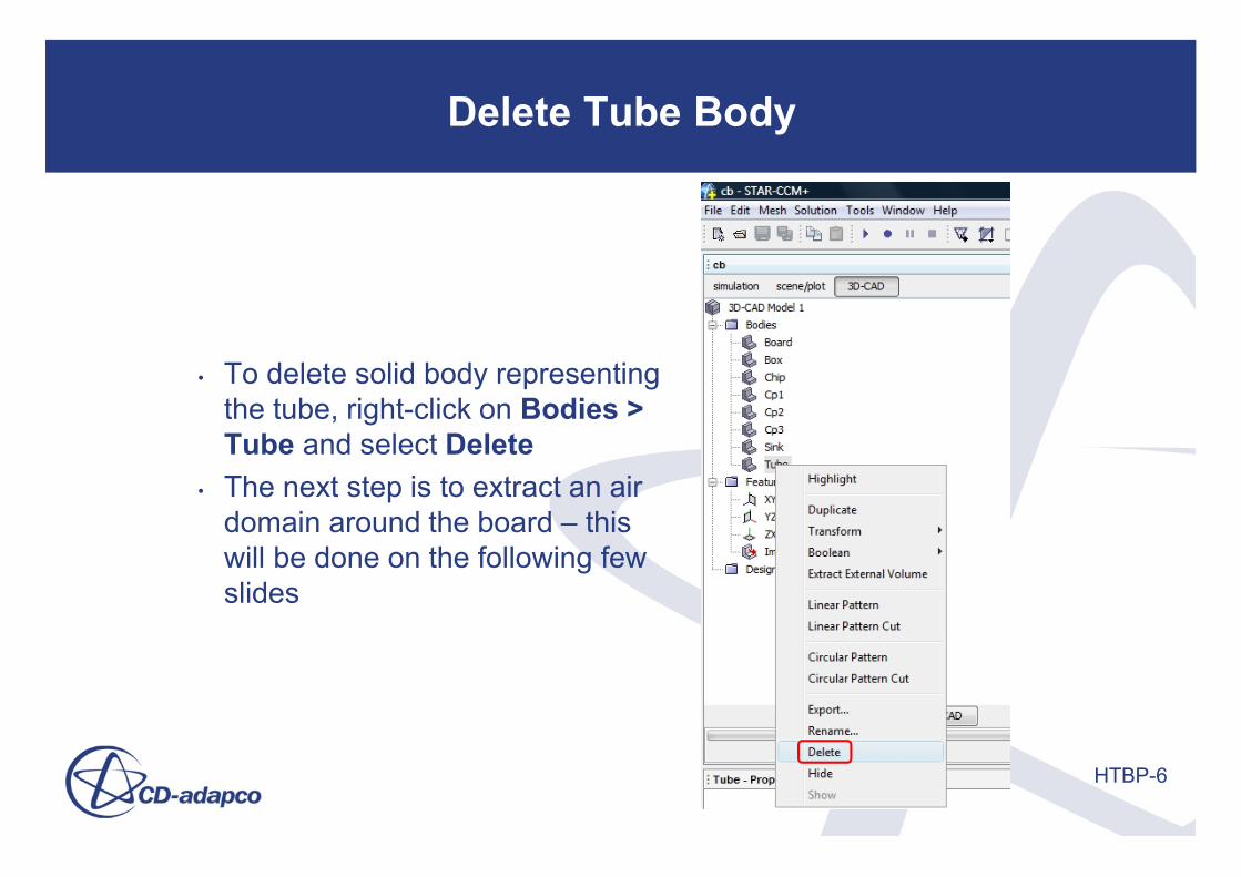
Delete Tube Body

• To delete solid body representing the tube, right-click on Bodies > Tube and select Delete

• The next step is to extract an air domain around the board – this will be done on the following few slides

HTBP-7

Create Sketch

• Right-click on the top surface of the board to highlight it (see adjacent image) and select Create Sketch

• This allows you to draw a new sketch on the planar surface defined by the board top surface

• Click the Create Rectangle button and create a rectangular sketch as follows:

• Lower left corner: (-0.07, -0.07)• Upper right corner: (0.25, 0.07)

• Click OK

HTBP-8

Extrude Block

• To create an extruded block, right click on Sketch 1 and select Features > Create Extrude

• In the Extrude window, set the Distance and Body Interaction as shown, then click OK

• A new body named Body 9 has been created

HTBP-9

Extract External Volume & Delete Original Block

• Now we will extract the air domain from the extruded body that was just created

• Right-click on Bodies > Body 9 and select Extract External Volume, then click OK

• A new body has been created; rename it to Air

• Delete Body 9, since it is no longer needed

HTBP-10

Best Practices: Geometry & Meshing

• The current best practice for conjugate heat transfer is to use a conformal mesh

• Conformal meshes have faces that match exactly one-to-one at interfaces• This ensures that heat transfer occurs smoothly across the interface• Requires imprinting of geometry surfaces on each other• Conformal meshes can only be generated by the Polyhedral Mesher (though it is

not guaranteed!)• Alternative approach is to use non-conformal meshes with in-place interfaces

• Matching will be extremely good, if not perfect, along flat interfaces• Non-matching faces at interfaces are most likely to occur on curved interfaces

with dissimilar mesh densities on either side• Interface matching can be improved by adjusting the Intersection Tolerance

(default is 0.05): higher values should result in more faces matching, though values that are too large can adversely impact mesh quality

• The Trimmed Mesher will always generate non-conformal meshes

HTBP-11

Best Practices: Conformal vs. Non-Conformal

Conformal

Non-Conformal

HTBP-12

Indirect Mapped Interfaces Demo

• New approach available in STAR-CCM+ v7.02: Non-conformal meshes with indirect mapped interfaces

• Improves interface matching robustness and likelihood of 100% matching• Currently available for fluid/solid and solid/solid interfaces (not yet compatible with

fluid/fluid interfaces or finite-volume stress)

HTBP-13

Best Practices: Thin-Walled Bodies

• When in-plane conduction can be neglected, contact interfaces can be used at fluid-solid or solid-solid interfaces, and baffle interfaces can be used at fluid-fluid interfaces

• When in-plane conduction is important, the Thin Mesher and Embedded Thin Mesher are available for meshing thin-walled bodies

• Both will generate a prismatic type mesh in geometries that are predominantly thin or have thin structures included in them

• The Thin Mesher will produce a non-conformal mesh• The Embedded Thin Mesher will produced a conformal mesh under certain conditions,

generally when the thin region is completely embedded within another region• New approach available in STAR-CCM+ v7.02: Shell Modeling

• Allows for the simulation of thin solids where lateral (in-plane) conductivity is important• Automatically created from a boundary – new shell region and interfaces are generated• Single or multiple shell layers may be modeled• Currently permit only isotropic thermal conductivity

HTBP-14

Shell Modeling Demo

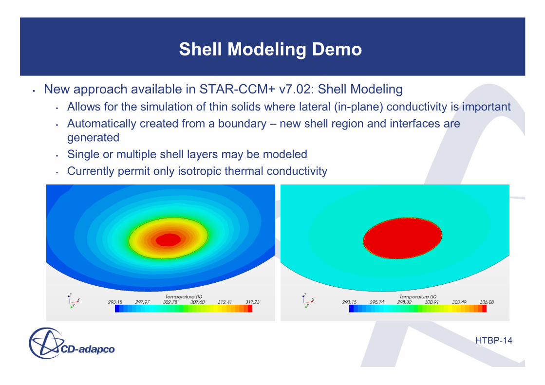
• New approach available in STAR-CCM+ v7.02: Shell Modeling• Allows for the simulation of thin solids where lateral (in-plane) conductivity is important• Automatically created from a boundary – new shell region and interfaces are

generated• Single or multiple shell layers may be modeled• Currently permit only isotropic thermal conductivity

HTBP-15

Imprint Bodies

• To create a conformal mesh we need to imprint the bodies on each other

• Select all of the bodies (using the Shift key), then right-click and select Boolean > Imprint

• Accept the default Imprint Type (Precise) and the click OK

HTBP-16

Rename Surfaces

• We will now rename some of the surfaces

• We could also wait until later to do this, but it is most convenient to do it now

• Right-click on the short side of the Air body that is closest to the Board, select Rename and set the name to Inlet

• Similarly, rename the opposite side to Outlet

• Click on Close 3D-CAD

HTBP-17

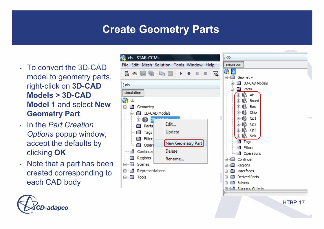
Create Geometry Parts

• To convert the 3D-CAD model to geometry parts, right-click on 3D-CAD Models > 3D-CAD Model 1 and select New Geometry Part

• In the Part Creation Options popup window, accept the defaults by clicking OK

• Note that a part has been created corresponding to each CAD body

HTBP-18

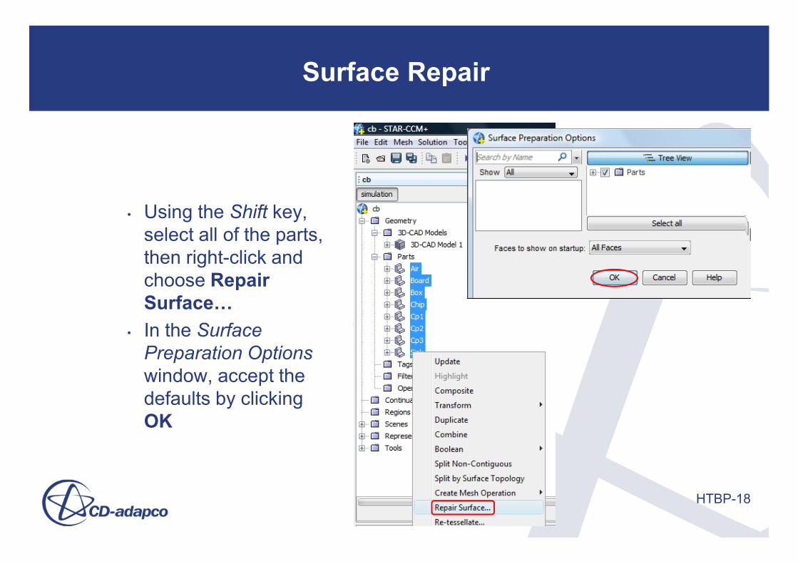
Surface Repair

• Using the Shift key, select all of the parts, then right-click and choose Repair Surface…

• In the Surface Preparation Options window, accept the defaults by clicking OK

HTBP-19

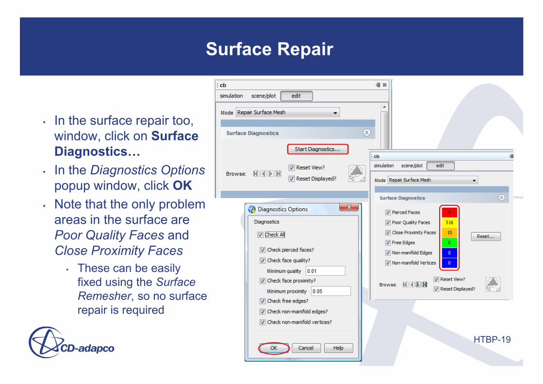
Surface Repair

• In the surface repair too, window, click on Surface Diagnostics…

• In the Diagnostics Optionspopup window, click OK

• Note that the only problem areas in the surface are Poor Quality Faces and Close Proximity Faces

• These can be easily fixed using the Surface Remesher, so no surface repair is required

HTBP-20

Create Regions from Parts

• We can now create regions from the geometry parts in preparation for meshing

• Select all of the parts, then right-click and select Assign Parts to Regions…

• Set the Region Mode, Boundary Mode and Feature Curve Mode as shown then click Create Regions

• Note that multiple regions, boundaries and interfaces have been created

HTBP-21

Define Mesh Continuum

• To begin the meshing process, start by defining a new mesh continuum and associated mesh models

• Right-click on Continua and select New > Mesh Continuum

• A new mesh continuum named Mesh 1 has been created

• Right-click on Continua > Mesh 1 and choose Select Meshing Models…

• Select the Surface Remesher, Prism Layer Mesher and Polyhedral Mesher as shown

HTBP-22

Best Practices: Wall Treatments

• Wall treatment models are used in conjunction with RANS models

• Three wall treatment options are available in STAR-CCM+:

– High-y+ wall treatment: equivalent to the traditional wall function approach, in which the near-wall cell centroid should be placed in the log-law region (30 ≤ y+ ≤ 100)

– Low-y+ wall treatment: suitable only for low-Re turbulence models in which the mesh is sufficient to resolve the viscous sublayer (y+ ≈ 1) and 10-20 cells within the boundary layer

– All-y+ wall treatment: a hybrid of the above two approaches, designed to give accurate results if the near-wall cell centroid is in the viscous sublayer, the log-law region, or the buffer layer

• Not all wall treatments are available for all RANS models

First grid point, 30 < y+ < 100 Viscous sublayer

First grid point y+ ~ 1

HTBP-23

Best Practices: Prism Layer Meshing

• Prism layers are mainly used to resolve flow boundary layers, so they are not needed at flow boundaries (e.g. inlets, outlets)

• Set proper boundary types prior to meshing and STAR-CCM+ will automatically disable prism layers at all flow boundaries

• Prism layers are mainly used to resolve flow boundary layers, so they are not generally required within solids

• Activate the Interface Prism Layer Option at all fluid-solid interfaces• Disable prism layers within all solid regions

• The All-y+ Wall Treatment offers the most meshing flexibility and is recommended for all turbulence models for which it is available (most of them)

• Follow the guidelines on y+ for different wall treatments as outlined on the preceding slide

– Build and run a coarse ‘test’ mesh to help estimate the proper near-wall mesh size– Estimate the y+ value for your problem using the procedure on the following slide

HTBP-24

Best Practices: Estimating y+

• We generally wish to target a specific value of y+ for the near-wall mesh, where:

• The wall shear stress τw can be related to the skin friction coefficient:

• The skin friction coefficient can be estimated from correlations– For a flat plate:

– For pipe flow:

νyuy

*

=+

ρτ wu ≈*

2/2UC w

f ρτ

=

5/1Re036.0

2 L

fC=

5/1Re039.0

2 D

fC=

HTBP-25

Example: Estimating y+

• For our electronics cooling problem, we will use an inlet velocity of 15 m/s. Using the air domain height of 5 cm as the characteristic length, along with the properties of air, we find

• Using the friction coefficient correlation for internal flow:

• The definition of the friction coefficient is used to compute the wall shear stress:

• The wall stress is used to compute u*:

• We will target a y+ of 80, so:

35/1 1006.9

Re039.0

2−×=⇒= f

D

f CC

22 /192.1

2/mN

UC w

wf =⇒= τ

ρτ

smu w /009.1* =≈ρ

τ

mmyyuy 25.1*

=⇒=+

ν

410743.4Re ×=D

HTBP-26

Mesh Reference Values

• Right-click on Continua > Mesh 1 > Reference Values and select Edit…

• Set the mesh values as shown in the adjacent screenshot

• Note that by using two prism layers with a total prism layer thickness of 2.5 mm and a stretching factor near 1, we will achieve a near-wall prism layer thickness close to our estimated value of 1.25 mm

HTBP-27

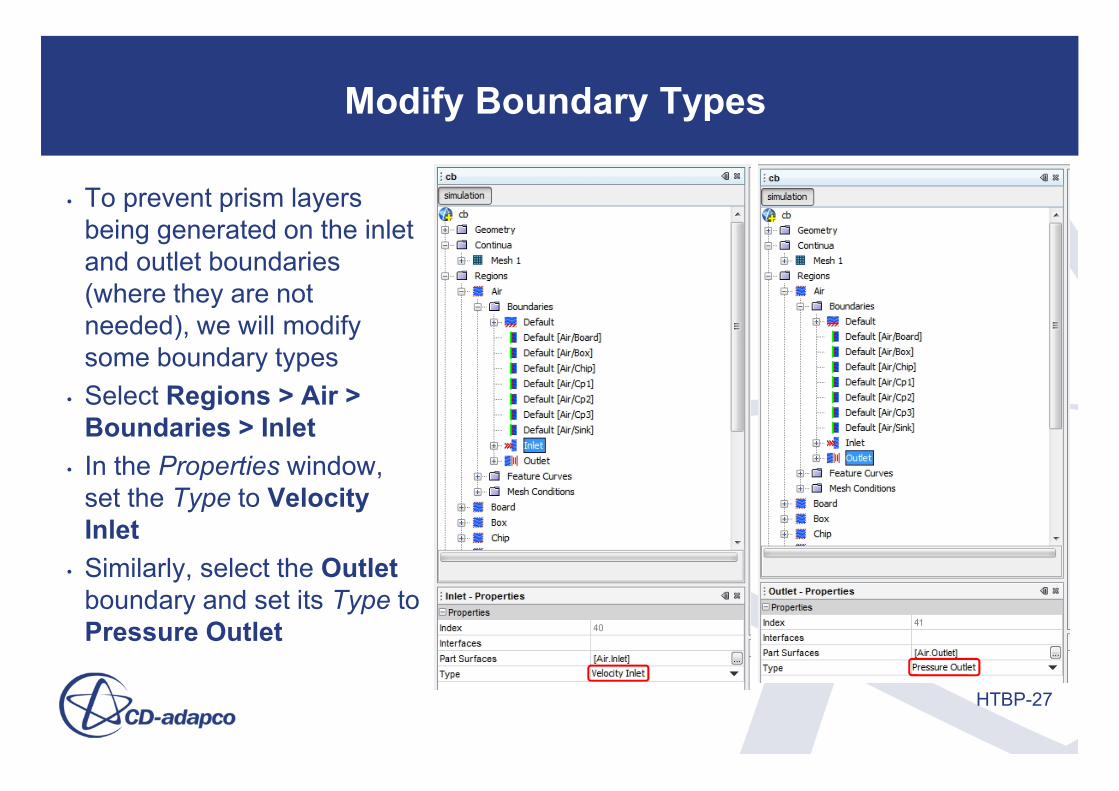
Modify Boundary Types

• To prevent prism layers being generated on the inlet and outlet boundaries (where they are not needed), we will modify some boundary types

• Select Regions > Air > Boundaries > Inlet

• In the Properties window, set the Type to Velocity Inlet

• Similarly, select the Outlet boundary and set its Type to Pressure Outlet

HTBP-28

Interface Prism Layers

• Since prism layers are not needed we will activate prism layer growth at the interfaces, but disable prism layers in the solid regions

• Under Interfaces, select all interfaces, then right-click and select Edit…

• Under Mesh Conditions > Interface Prism Layer Option, tick the Grow Prisms from Interface box

HTBP-29

Disable Prism Layers in Solid Regions

• Under Regions, select all of the solid regions (i.e. all except Air), then right-click and choose Edit…

• Under Mesh Conditions > Customize Prism Mesh, set Customize Prism Mesh to Disable

HTBP-30

Generate Mesh

• Generate the remeshed surface and volume mesh using the Generate Volume Mesh button on the Mesh Generation toolbar:

• Before proceeding check the mesh quality by selecting Mesh > Diagnostics… from the top menu, then clicking OK in the Mesh Diagnostics popup window

• The results at the right show that the mesh quality is very good

HTBP-31

Examine Mesh

• Make a few plots of the mesh as shown

• Although fairly coarse, the mesh density is adequate for the purposes of this demonstration

• The resulting volume mesh consists of approximately 108K cells

HTBP-32

Air Physics Continuum

• Under Continua, change the name of the Physics 1 continuum to Air

• Right-click on Continua > Air and choose Select Models…

• Select the physics models as shown

HTBP-33

Copper Physics Continuum

• Right-click on Continua and select New > Physics Continuum

• Change the name of the newly-defined continuum to Copper

• Select the physics models as shown in the screenshot below

• Right-click on Continua > Copper > Models > Solid > Al and select Replace with…

• Select Material Databases > Standard > Solids > Cu (Copper) to change the material properties

HTBP-34

Silicon Physics Continuum

• Right-click on Continua and select New > Physics Continuum

• Change the name of the newly-defined continuum to Silicon

• Select the physics models as shown in the screenshot below

• Right-click on Continua > Silicon > Models > Solid > Al and select Replace with…

• Select Material Databases > Standard > Solids > Si (Silicon) to change the material properties

HTBP-35

Modify Region Physics Continua

• Select all of the regions except for Air and Sink

• In the Properties window, set the Physics Continuum to Silicon

• Similarly, select the Sink region and change its Physics Continuum to Copper

HTBP-36

Box Volume Report

• We will now create a report to output the volume of the Box region

• Right-click on Reports and select New Report > Sum

• Rename this new report to Box Volume

• Define the properties of the report as shown

• Note that a new field function named Report: Box Volume has been automatically defined

HTBP-37

Best Practices: Internal Heat Sources

• Internal heat sources can be applied within materials in two different ways• Volumetric sources • Interfacial sources

• Volumetric sources are applied within the volume of a region• Enable Energy Source Options under region’s Physics Conditions• Specify Method (constant, table, field function, user code) under region’s Physics

Values• Input values have units of power per unit volume

• Interface heat sources are applied at a fluid-solid or solid-solid contact interface• Enable Energy Source Options under interface’s Physics Conditions• Specify Method (constant, table, field function, user code) under interface’s Physics

Values• Input values have units of power per unit area

HTBP-38

Best Practices: Thermal Contact Resistance

• Thermal contact resistance is often important between parts in which the contact is not perfect

• Depends on factors such as surface roughness, flatness and cleanliness, as well as interstitial materials and contact pressure

• Results in a temperature discontinuity at the interface• Can be modeled in STAR-CCM+ but contact resistance values must be supplied by

the user (i.e. STAR-CCM+ cannot predict these values)• ‘Contact’ resistance can also be specified at a fluid-solid interface (e.g. to model a

thin coating or fouling layer)

• Contact resistance is applied at contact interfaces• Conduction is purely one-dimensional (no in-plane conduction)• Specify Method (constant, table, field function, user code) under interface’s Physics

Values• Input values have units of m^2-K/W

HTBP-39

Box Heat Source Field Function

• Next, we define a new field function to set the box volumetric heat source

• Right-click on Tools > Field Functions and select New

• Rename the newly-created field function to Box Heat Source

• Set the Function Name to BoxHeatSourceand set the Dimensions as shown

• Set the field function Definition as shown• This will be used to distribute 70 W of

power uniformly throughout the Box region volume

HTBP-40

Box Heat Source

• Select Regions > Box > Physics Conditions > Energy Source Option

• In the Properties window, select Volumetric Heat Source for the Energy Source Option

• Right-click Regions > Box > Physics Values and select Edit…

• In the edit window, select Physics Values > Energy Source and set the Method to Field Function and the Scalar Function to Box Heat Source

HTBP-41

Board-Chip Interface Heat Generation

• Under Interfaces, select all of the interfaces and make sure that the Type for each is set to Contact Interface

• Next, right-click on the Board/Chipinterface and select Edit…

• Under Physics Values > Heat Flux, set the Value to 50000 W/m^2

• This will provide the specified interface heat generation rate with the fraction of heat traveling into the Chip and Board regions according to their respective thermal resistances

HTBP-42

Box-Board Thermal Contact Resistance

• A thermal contact resistance will be applied between the Board and Box regions

• Select Interfaces > Board/Box > Physics Values > Contact Resistance > Constant

• In the Properties window, set the Value to 1.e-4 m^2-K/W

HTBP-43

Best Practices: S2S Thermal Radiation

• Used to simulate gray (wavelength-independent) diffuse thermal radiation exchange between surfaces forming a enclosure

• Medium between surfaces must be non-participating• When all solids are opaque in a CHT problem (a

common occurrence), thermal radiation needs to be activated only for the fluid domain(s)

• Requires the definition of radiation patches and the availability of view factors between these patches

– Radiation patches are groups of boundaries which form a continuous portion of a surface

– View factor Fij is the proportion of radiation leaving a patch i that strikes another patch j

jiA Aij

ji

iij dAdA

RAF

i j∫ ∫= 2

coscos1π

θθ

HTBP-44

Best Practices: S2S Radiation Patches

• Default behavior is that each cell face corresponds to a patch

• This can lead to a prohibitive number of patches on larger models

• Number of patches can be controlled using the patch/face proportion or by specifying a target total number of patches

• The patch/face proportion specifies the (approximate) percentage of each patch occupied by one cell face

• e.g. a patch/face proportion of 25.0 (a commonly-used value) would correspond to each patch consisting of 4 cells faces, on average

• Each color is a different patch• Note that multiple cell faces form

each patch

HTBP-45

Best Practices: S2S Radiation Properties

• Thermal radiation properties to be specified for non-participating media are:– Emissivity ε– Absorptivity α– Reflectivity ρ– Transmissivity τ

• From energy conservation, α + ρ + τ = 1• From Kirchhoff’s Law, α = ε

– Kirchhoff’s law states that the emissivity of a surface at temperature T equals the absorptivity by that surface of radiation from a black body at the same temperature

– Therefore, Kirchhoff’s law is not true in general for radiation from surfaces at differing temperatures, but it is usually assumed to be valid

• Note that for opaque surfaces (τ = 0), assuming Kirchhoff’s Law to be valid and using energy conservation, only one independent radiation property (ε) needs to be specified

HTBP-46

Set Patch/Face Proportion

• We will now set the patch/face proportion which will control the number of radiation patches in the model

• Select Regions > Air > Physics Values > Patch/Face Proportion and set the Patch/Face Proportion to 25.0

• This will have the effect of each patch consisting of 4 cells faces, on average

HTBP-47

Copper Sink Emissivity

• Next we will set the emissivities of the surfaces

• Note that since all solids are opaque, thermal radiation is active only for the air region, so all radiation properties are set within the Air region

• We will assume the silicon emissivity to be 0.8 (the default value) and the copper emissivity to be 0.1

• Select Regions > Air > Boundaries > Default (Air/Sink) > Physics Values > Surface Emissivity > Constant and set the Value to 0.1

HTBP-48

Inlet & Outlet Boundary Conditions

• Right-click on Regions > Air > Boundaries > Inlet and select Edit…

• The Static Temperature and Radiation Temperature can be left at their default values of 300 K in this case

• Set the value of the Velocity Magnitude to 15.0 m/s

HTBP-49

1/h

Best Practices: Thermal Boundary Conditions

• For wall boundaries which are not solid-fluid or solid-solid interfaces (i.e. true boundaries), the following choices are available:

– Adiabatic walls (zero heat transfer)– Fixed wall heat flux– Fixed wall temperature– Convection: see adjacent image

• For S2S thermal radiation, the domain must form an enclosure, so flow boundaries (e.g. inlets, pressure outlets) must have environmental patches and boundary conditions

• Boundary conditions are specified as “radiation temperatures”• Radiation temperatures do not have to be the same as the

temperature of the flow crossing the boundary• Radiation temperature should represent the temperature to

which radiation from the model is transmitted

HTBP-50

Board Thermal Boundary Conditions

• We set the side and bottom boundaries of the Board region to have convective heat transfer boundary conditions

• Right-click on Regions > Board > Boundaries > Defaultand select Edit…

• Under Physics Conditions > Thermal Specification, set the Method to Convection

• Under Physics Values, set theAmbient Temperature to 300 K and the Heat Transfer Coefficient to 100 W/m^2-K

HTBP-51

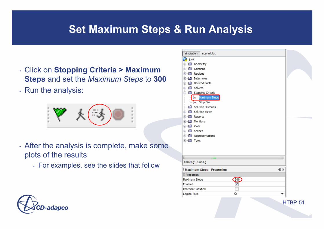
Set Maximum Steps & Run Analysis

• Click on Stopping Criteria > Maximum Steps and set the Maximum Steps to 300

• Run the analysis:

• After the analysis is complete, make some plots of the results

• For examples, see the slides that follow

HTBP-52

Convergence History

HTBP-53

Wall y+

• Note that our estimate resulted in y+ values in the proper range for the high-y+ wall treatment

• However, the values are a bit low compared to our targeted value

• Many of the lower y+ regions are in areas where the flow is impinging on the surface or has separated from the surface

• There is no boundary layer there!

HTBP-54

Best Practices: Heat Transfer Coefficients

• The convective heat transfer coefficient (HTC) is defined as:

• The only term not clearly specified is the fluid temperature, i.e. the fluid temperature where?

• The choice of fluid temperature may be used to define different heat transfer coefficients

– Some definitions may be more useful than others– For turbulent forced convection, we would like the HTC to depend on the

Reynolds’ number, fluid properties and geometry– There may also be some sensitivity to the type of boundary condition (i.e.

fixed temperature vs. constant heat flux), but the HTC should not depend on the value of the boundary condition

– The above will be true only for particular choices of the fluid temperature

( )fluidwall

wall

TTqh−′′

=

HTBP-55

Best Practices: STAR-CCM+ HTCs

• Heat Transfer Coefficient:• Uses the computed wall heat flux, wall temperature, and a fluid temperature

specified by the user• Does not account for local variations in fluid temperature

• Local Heat Transfer Coefficient:• Uses definitions from the wall treatment to compute a heat transfer coefficient• These definitions effectively use the near-wall fluid cell temperature• May have some sensitivity to near-wall mesh size

• Specified y+ Heat Transfer Coefficient:• Uses a fluid temperature at a specified y+ value• Accommodates local fluid temperature variation effects• Eliminates sensitivity to near-wall mesh size• Recommended as best practice - combines the best features of the Heat Transfer

Coefficient and the Local Heat Transfer Coefficient

HTBP-56

Heat Transfer Coefficient

Can have negative values

HTBP-57

Local HTC

HTBP-58

Specified y+ Heat Transfer Coefficient (y+ = 100)

Recommended

HTBP-59

Summary

• We have worked through a simplified conjugate heat transfer problem with a number of features typically encountered in real industry problems

• Best practices for the following topics have been demonstrated and discussed:

• Imprinting and CHT Interfaces• New STAR-CCM+ v7.02 Features for CHT• Wall Treatments and Near-Wall Meshing• Internal Heat Generation• Thermal Contact Resistance• Thermal Radiation• Thermal Boundary Conditions• Heat Transfer Coefficients