heat transfer laboratory lab manual list of …

Department of Chemical Engineering, Veer Surendra Sai University of Technology Burla

1

HEAT TRANSFER LABORATORY

LAB MANUAL

LIST OF EXPERIMENTS:

1. To find out the overall thermal conductance and plot the temperature distribution in case of a

composite wall

2. To determine the thermal conductivity of a liquid.

3. To find out the temp. Distribution along the length of a Pin Fin under free convection

4. To find out the temp. Distribution along the length of a Pin Fin under forced convection

5. To find out the Heat Transfer Coefficient of vertical cylinder in natural convection.

6. To find out the Stefan Boltzmann constant.

7. To calculate the overall heat transfer coefficient for parallel flow heat exchanger.

8. To calculate the overall heat transfer coefficient for counter current flow heat exchanger.

9. To find the heat transfer co-efficient for Drop-wise condensation.

10. To find the heat transfer co-efficient for Film-wise condensation process.


2

EXPERIMENT-1

OBJECTIVE: Study of conduction heat transfer in composite wall.

AIM:

1. To determine total thermal resistance and thermal conductivity of composite wall.

2. To calculate thermal conductivity of one material in composite wall.

3. To plot the temperature profile along the composite wall.

INTRODUCTION:

When a temperature gradient exists in a body, there is an energy transfer from the high

temperature region to the low temperature region. Energy is transferred by conduction and heat

transfer rate per unit area is proportional to the normal temperature gradient:

X

T

A

q

When the proportionality constant is inserted,

X

TkAq

Where q is the heat transfer rate and T/ X is the temperature gradient in the direction of heat

flow. The positive constant k is called thermal conductivity of the material.

THEORY:

A direct application of Fourier’s law is the plane wall. Fourier’s equation:

12 TTX

kAq

Where the thermal conductivity is considered constant. The wall thickness is X, and 1T

and 2T are surface temperatures. If more than one material is present, as in the multiplayer

Wall, the analysis would proceed as follows:

The temperature gradients in the three materials (A, B, C), the heat flow may be written

C

CC

B

BB

A

AA

X

TAk

X

TAk

X

TAkq


3

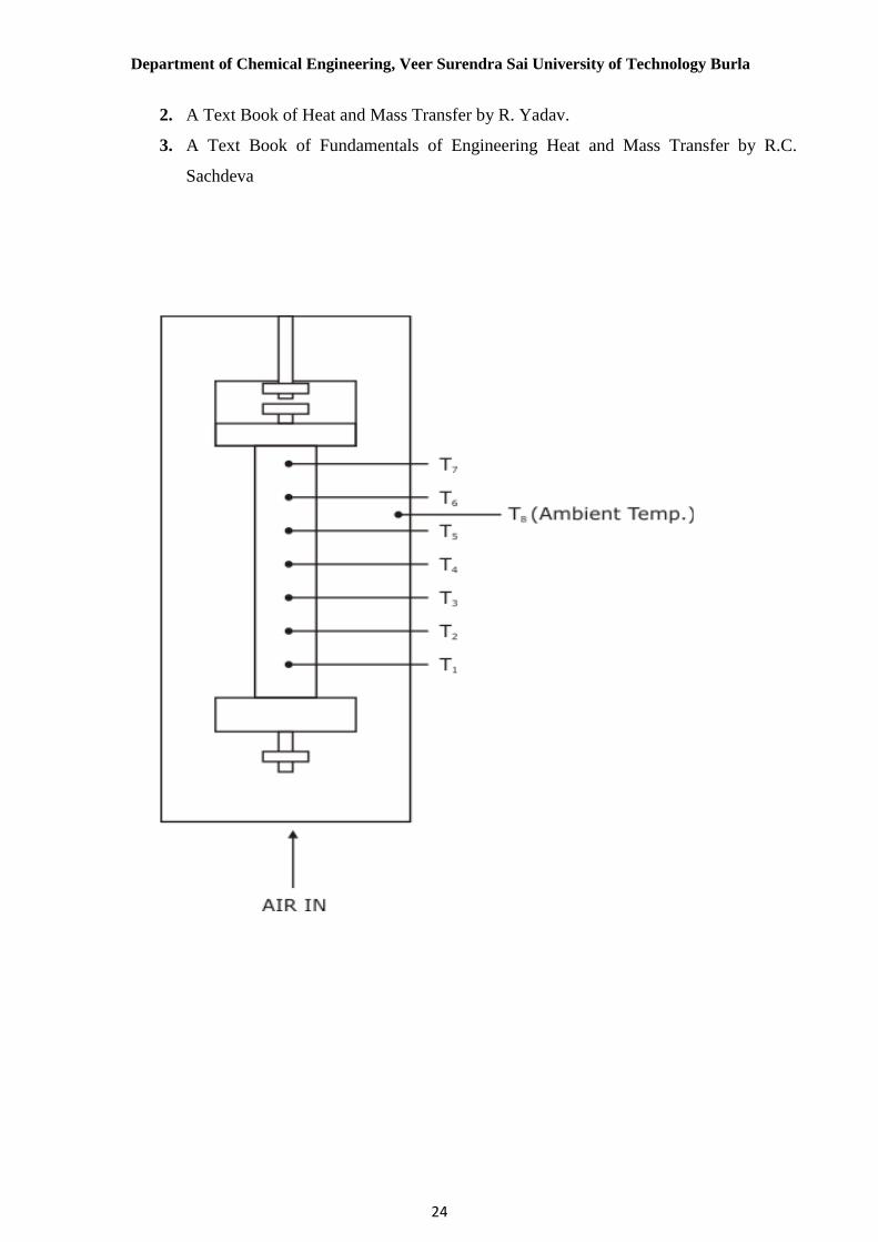
DESCRIPTION:

The Apparatus consists of a heater sandwiched between two asbestos sheets. Three slabs of

different material are provided on both sides of heater, which forms a composite structure. A

small press- frame is provided to ensure the perfect contact between the slabs. A Variac is

provided for varying the input to the heater and measurement of input power is carried out by a

Digital Voltmeter & Digital Ammeter. Temperatures Sensors are embedded between inter faces

of the slab, to read the temperature at the surface. The experiment can be conducted at various

values of power input and calculations can be made accordingly.

UTILITIES REQUIRED:

1. Electricity Supply: Single Phase, 220 VAC, 50 Hz, 5-15Amp socket with earth

connection.

2. Bench Area Required: 1m x 1m.

EXPERIMENTAL PROCEDURE:

STARTING PROCEDURE:

1. Ensure that Mains ON/OFF switch given on the panel is at OFF position &dimmer-stat is

at zero position.

2. Connect electric supply to the set up.

3. Switch ON the Mains ON / OFF switch.

4. Set the heater input by the dimmer-stat, voltmeter in the range 40 to 100 V.

5. After 1 hour. Note down the reading of voltmeter, ampere meter and temperature sensors

in the observation table after every 10 minutes interval till observing change

inconsecutive readings of temperatures (± 0.2 oC).

CLOSING PROCEDURE:

1. After experiment is over set the dimmer stat to zero position.

2. Switch OFF the Mains ON/OFF switches.

3. Switch OFF electric supply to the set up.

OBSERVATION & CALCULATIONS:

DATA:

d = 0.25 m


4

X1 = 0.020 m = 20mm

X2 = 0.020m = 20 mm

X3 = 0.012m = 12mm

K1=125w/m℃

K2=1.4w/m℃

K3=----w/m℃

OBSERVATION TABLE:

Sl. No V

Volts

A

Amps

T1

oC

T2

oC

T3

oC

T4

oC

T5

oC

T6

oC

T7

oC

T8

oC

CALCULATIONS:

To plot the temperature profile,

Distance 0 10 20 45

Avg. Temp

At distance 0, average temp

2

21 TT


2

43 TT


2

65 TT


2

87 TT

Heat supplied by the heater, IVW 86.0 , watts

Amount of Heat Transfer, Q = W, watts


5

Where, 2

4dA

, m2

Overall Temp. Difference

2

8271 TTTTT

, oC

Total thermal resistance of composite wallq

TRt

, oC m2/W

Total thickness of wall 321 XXXX , m

Thermal Conductivity of composite wallT

XqKeff

, W/m oC

Thermal Conductivity of press wood

2

2

1

1

33

k

X

k

X

q

T

XK , W/m oC

NOMENCLATURE:

A = Area of heat transfer, m2

d = Diameter, m

I = Ammeter reading, amp

K eff = Thermal conductivity of composite wall, W/m oC

k1 = Thermal conductivity of cast iron, W/m oC

. k2 = Thermal conductivity of Press wood, W/m oC

k3 = Thermal conductivity of Bakelite, W/m oC

Q = Amount of heat transfer, W

q = Heat flux, W/m2

Rt = Total thermal resistance of composite wall, oC m2/W

ΔT = Overall temperature difference, oC

T1 & T2 = Interface temperature of 1ST slab and heater, oC

T3 & T4 = Interface temperature of 1st and2nd slab, oC

T5 & T6 = Interface temperature of 2nd and 3rd slab, oC

T7 & T8 = Top surface temperature of press wood, oC

V = Voltmeter reading, volts

W = Heat supplied by the heater, W


6

ΔX = Total thickness of wall, m

X1 = MS Slab thickness, m

X2 = Bakelite slab thickness, m

X3 = Press wood thickness, m

PRECAUTION

1. Use the stabilize A.C. Single phase supply only. The voltage should not very more than +

volts

2. Keep Dimmer stat to zero before start and increase the voltage slowly.

3. Keep all the assembly undisturbed.

4. Remove air gap between plates by moving hand press gently.

5. Operate selector switch of temperature indicator gently.

There is a possibility of getting abrupt result if the supply voltage fluctuating or if the

satisfactory steady state condition is not reached.


7

EXPERIMENT-2

OBJECTIVE:

Study of heat transfer through liquid

AIM:

To determine the thermal conductivity of a liquid

INTRODUCTION:

When temperature gradient exists in a body, there is an energy transfer from the high

temperature region to the low temperature region. Energy is transferred by conduction and

heat transfer rate per unit area is proportional to the normal temperature gradient:

𝑞

𝐴≈

𝜕𝑇

𝜕𝑋

When the proportionality constant is inserted,

q = −KA ∂T

∂X

Where q is the heat transfer rate and ∂T ∕ ∂X is the temperature gradient in the direction of

heat flow. The positive constant k is called is thermal conductivity of the material.

THEORY:

For thermal conductivity of liquids using Fourier’s law, the heat flow through the

liquid from hot fluid to cold fluid is the heat transfer through conductive fluid medium.

Fourier’s equation:

q =−KA

∆X(T1 − T2)

Fourier’s law for the case of liquid

At steady state, the average face temperatures are recorded (Th and Tc) along with the

rate of heat transfer (Q). Knowing, the heat transfer area (Ah) and the thickness of the sample

(∆X) across which the heat transfer takes place, the thermal conductivity of the sample can be

Calculated using Fourier’s Law of heat conduction.

Q = kAh ΔT/ΔX = kAh (Th - Tc) / ΔX


8

Th

q

Δx

Heat transfer area = Ah (area to direction of heat flow)

DESCRIPTION:

The apparatus is based on well-established “Guarded Hot Plate” method. It is a steady

state absolute method suitable for materials, which can be fixed between two parallel plates

and can also be extended to liquids that fill the gap between the plates.

The essential components of the set-up are the hot plate, the cold plate, and heater to

heat the hot plate, cold water supply for the cold plate, RTD PT-100 Sensors and the liquid

specimen holder.

In the set-up, a unidirectional heat flow takes place across the liquid whose two faces are

maintained at different temperatures by the hot plate on one end and by the cold plate at the

other end.

A heater heats hot plate and voltage to the heater is varied with the help of variac to

conduct the experiment on different voltages as well as different heat inputs. Temperatures are

measured by RTD PT-100 sensors attached at three different places on the hot plate as well as

on the cold plate. These sensors are provided on the inner surface facing the liquid sample. An

average of these sensor readings are used as Th and Tc at steady state condition.

Heat is supplied by an electric heater for which, we have to record the voltmeter reading

(V) and ammeter reading (A) after attaining the steady state condition. The temperature of the

cold surface is maintained by circulating cold water at high velocity. The gap between hot plate

and cold plate forms the liquid cell, in which liquid sample is filled.

The depth of the liquid in the direction of flow must be small to ensure the absence of

convection currents and a liquid sample of high viscosity and density shall further ensure the

absence of convection and the heat transfer can be safely assumed to take place by conduction

alone.


9

UTILITIES REQUIRED:

Water supply 5 lit/min (approx.)

Drain.

Electricity Supply: 1 Phase, 220 V AC, 2 Amperes.

Table for set-up support (optional)


1. Fill the liquid cell with the sample liquid (glycerol) through the inlet port, keeping the

apparatus tilted towards upper side so that there is complete removal of air through the

outlet port. Liquid filling should be continued till there is complete removal of air and also

liquid glycerol comes out of the outlet port. Close the outlet port followed by inlet port.

2. Allow cold water to flow through the cold-water inlet.

3. Start the electric heater to heat hot plate. Adjust the voltage of hot plate heater in the range

of 10 to 50 volts.

4. Adjust the cold-water flow rate such that there is no appreciable change the outlet

temperature of cold water (there should be minimum change).

5. Go on recording the thermocouple readings on hot side as well as on cold side, and once

steady state is achieved (may be after 30-60 min); (steady state is reached when there no

appreciable change in the thermocouple readings, 0.1,°C), record the three thermocouple

readings (Th1, Th2, Th3 i.e. T1, T2, T3 on Temperature Indicator) on the hot side and

three thermocouple readings (Tc1, Tc2, Tc3 i.e. T4, T5, T6 on Temperature Indicator)

on the cold side along with the voltmeter (V) and ammeter (A) readings.

6. Stop the electric supply to the heater, and continue with the supply of cold water till there

is decrease in temperature of hot plate (may be for another 30-40 min).

7. Open the liquid outlet valve slightly in the downward tilt position and drain the sample

liquid in a receiver, keeping liquid inlet port open.

SPECIFICATION:

1. Hot Plate


10

Material = brass

Diameter = 180 mm

2. Cold Plate

Material = Aluminum

Diameter = 180 mm

3. Sample Liquid depth = 18 mm

4. Temp. Sensors = RTD PT-100 type.

Type = RTD PT-100 type

Quantity = 6 Nos.

No. 1 to No. 3 mounted on hot plate.

No. 4 to No. 6 mounted on cold plate.

5. Digital Temperature indicator

Range = 0°C to 199.9°C

Least Count = 0.1o

C

6. Variac = 2 Amp, 230VAC

7. Digital Voltmeter = 0 to 250 Volts

8. Digital Ammeter = 0 to 2.5 Amp.

9. Main Heater = Nichrome heater 300 Watt approximate, ring

heater mica held between plates 300 watt, top

heater held between plates 300 watt, separate

dimmer for heaters, volt and current meter, multi-

channel digital temp indicator

FORMULAE

1. Heat input,

Q =V*I watt


11

2. Thermal conductivity of liquid,

K = Q ∆X

A(Th−Tc), Watt/m°C

OBSERVATIONS & CALCULATIONS:

DATA:

Effective diameter of plate = 0.165 m

Effective area of heat transfer, A = 0.02139 m2

OBSERVATIONS TABLE:

Sl. No. V I W Th1 Th2 Th3 TC1 TC2 TC3 Cold water flow rate

Record the following at steady state:

Sample liquid:

Heat input, Q = -------------- watt

Hot face average temperature, Th = (Th1 + Th2 +Th3) /3

Cold face temperature, Tc = (Tc1 + Tc2 + Tc3) / 3

Temperature difference, ΔT = (Th-Tc)

Thermal conductivity, K = ------------- W/m °C

NOMENCLATURE:

Q = Heat supplied by heater, watt.

A = Heat transfer area, m2

Th = Hot face average temperature, °C

Tc = Cold face average temperature, °C

∆T = Temperature difference, °C

K = Thermal conductivity of liquid, w/m, °C


12

ΔX = Thickness of liquid, mm = 18 mm

PRECAUTIONS & MAINTENANCE INSTRUCTIONS:

1. Use the stabilize A.C. Single Phase supply only.

2. Never switch on mains power supply before ensuring that all the ON/OFF switches

given on the panel are at OFF position.

3. Voltage to heater starts and increases slowly.


5. Never run the apparatus if power supply is less than 180 volts and above than 240

volts.


7. Always keep the apparatus free from dust.

8. Testing liquid should be fully filled.

There is a possibility of getting abrupt result if the supply voltage is fluctuating or if the

satisfactory steady state condition is not reached.

TROUBLESHOOTING:

1. If electric panel is not showing the input on the mains light. Check the fuse and also

check the main supply.

2. If D.T.I displays “1” on the screen checks the computer sockets if loose tight it.

3. If temperature of any sensor is not displays in D.T.I check the connection and rectify

that.

4. Voltmeter showing the voltage given to heater but ampere meter does not. Tight the

heater socket & switch if ok it means heater burned and replace that.

REFERENCES:

1. Holman, J.P., “Heat Transfer”,8th ed., McGraw Hill, NY, 1976.

2. Kern, D.Q., “Process Heat Transfer”, 1st ed., McGraw Hill, NY, 1965.

3. Perry, R.H., Green, D.(editors), “Perry’s Chemical Engineers’ Handbook”, 6th ed.,

McGraw Hill, NY, 1985.

4. McCabe, W.L., Smith, J.C., Harriott, P., “Unit Operations of Chemical

Engineering”, 4th ed. McGraw Hill, NY, 1985.

5. Coulson, J.M., Richardson, J.F., “Coulson & Richardson’s Chemical Engineering

Vol. - 1”, 5th ed., Asian Books ltd., ND, 1996.


13

EXPERIMENT-3 & 4

AIM:

To study the temperature distribution along the length of a pin under free convection heat

transfer.

INTRODUCTION:

Extended surfaces or fins are used to increase the heat transfer rate from a surface to a fluid

wherever it is not possible to increase the value of the surface heat transfer coefficient or the

temperature difference between the surface and the fluid. The use of this is very common and

they are fabricated in a variety of shapes (Fig.1) circumferential fins around the cylinder of a

motor cycle engine and fins attached to condenser tubes of a refrigerator are few familiar

examples.

FAMILIAR EXAMPLES:

It is obvious that a fin surface sticks out from primary heat transfer surface. The temperature

difference with surrounding fluid will steadily diminish as one moves out along the fin. The

design of the fins therefore requires knowledge of the temperature distribution in the fin. The

main object of this experiment set up is to study the temperature distribution in a simple pin fin.

Fin effectiveness==tanh mL/mL

The temperature profile within a pin fin is given by:

/º = [T-Tf] / [Tb-Tf]= (Cosh m(L-x) + HSinh m (L-x) ] / [Cosh mL+HSinh mL]

where Tf is the free stream tem. Of air; Tb is the temp. of fin at its base; T is the temp. Within in

the fin at any x; L is the length of the fin and D is the fin diameter. M is the fin parameter defined

as:

fin parameter m= √ [hC/(kb A)]

kb=thermal conductivity of brass fin = 95 kcal/h-m-ºC

Where C= perimeter = π*D

A=cross-sectional area of fin= (/4) D2


14

APPARATUS:

A brass fin of circular cross section is fitted across a long rectangular duct. The other end of the

duct is connected to the suction side of a blower and the air flows past the fin perpendicular to its

axis. One end of the fin projects outside the duct and is heat by a heater. Temperature at five

points along the length of the fin is measured by RTD PT-100 type temperature sensors

connected along the length of the fin. The air flow rate is measured by an orifice meter fitted on

the delivery side of the blower.

SPECIFICATIONS: -

1. Dust size: -1800mm*100mm*100mm

2. Diameter of the fin: 12.7mm

3. Length of the fin: 150mm

4. Diameter of the pipe: 52mm

5. Diameter of the orifice: 26mm

6. Coefficient of discharge Cd: 0.64

7. Centrifugal blower: 1 phase motor

8. Temp. Indicator: 0-199.9°C, RTD PT-100 type

9. Thermal Conductivity of fin material (Brass):95 Kcal/hr-m-°c

10. Temp. Sensors No.6 reads ambient temp. in the inside of the Duct.

11. Dimmerstat for heat input control 230V, 2 Amps.

12. Voltmeter 0-250V

13. Ammeter 0-2A

NATURAL CONVECTION:

PROCEDURE:

1. Start heating the fin by switching on the heater element and adjust the voltage on dimmer

stat to say 60 volts (increase slowly from 0 onwards)

2. Note down the Temp. sensors readings No. 1 to 5

3. When steady state is reached, record the final readings of Temperature Sensor No.1 to 5

and also the ambient temperature reading, Temperature Sensor No.6

4. Repeat the same experiment with voltage =100 volts and 120 volts.


15

FORCED CONVECTIONS:

PROCEDURE

1. Start heating the fin by switching on the heater and adjust dimmerstat voltage equal to

100 volts.

2. Start the blower and adjust the difference of level in the manometer H=cm with the help

of valve.

3. Note down the Temperature Sensor readings (1) to (5) at a time interval of 5 minutes.

4. When the steady state is reached, record the final readings (1) to (5) and also record the

ambient temperature readings by (6)

5. Repeat the same experiment with H=cm etc.

OBSERVATIONS:

Experiment Power

Input,

W=V* I

FIN TEMPERATURE, OC Ambient

Temp.

Manometer

Reading,

H,

m of Water

T1 T2 T3 T4 T5 T6

x=3

cm

x=6

cm

x=9

cm

x=12

cm

x=15

cm

Forced

Convection

Free

Convection

CALCULATION:

FREE CONVECTION

EXPERIMENTALLY

5

54321 TTTTTTm

, oC


16

fm TTT , oC 6TT f

IVQ , W

dLAs , m2

TA

Qh

s

Exp

, W/m2 oC

THEORETICALLY

5

54321 TTTTTTm

, oC

fm TTT , oC 6TT f

2

fm

mf

TTT

, oC

15.273

1

mfT , 1/K

2

3

v

TDgGr

4/153.0 rru PGN

D

kNh airu

Theo

, W/m2oC

Ak

hCm

b

, m

DC , m2

2

4DA

, m2

mL

mLtanh

mK

hH

b

, m

mLHmlxLmHxLmTT

TT

fb

f

o

sinhcosh/sinhcosh,


17

Taking base temperature, Tb=T1

FORCED CONVECTION:

EXPERIMENTALLY

74.395

2.385.383.397.3943

5

54321

TTTTT

Tm , oC

74.63374.39 fm TTT , oC 6TT f

47.1225.09.49 IVQ , W

31098.515.00127.0 dLAs , m2

3.30974.61098.5

47.123

TA

Qh

s

Exp , W/m2 oC

THEORETICALLY

74.395

2.385.383.397.3943

5

54321

TTTTT

Tm , oC

37.362

3374.39

2

fm

mf

TTT , oC

32210123.2052.0

44

pp da , m2

42210309.5026.0

44

oo da , m2

67.86121.1

1000

100

7.82.191

100

21

a

whhH

, m

0144.0

1030.51012.2

67.8681.921030.51012.264.02

2423

43

22

op

opo

a

aa

HgaacQ

, m3/s

23.1141026.1

0144.0'

4

A

QV a , m/s

422 1026.10127.044

DA , m2

48.11515.273/15.273'1 fmf TTVV , m/s


18

31 1069.94

ae

DVR

18.1281069.94615.0466.03 uN

4.27202699.018.128

DD

KNh airu

Theo , W/m2oC

AK

hCm

b

, m

DC , m

mL

mLtanh

mK

hH

b

, m

mLHmlxLmHxLmTT

TT

fb

f

o

sinhcosh/sinhcosh,

Taking base temperature, Tb=T1

NOMENCLATURE:

ap = Area of pipe, m2

ao = Area of orifice, m2

A = Cross sectional area of fin, m2

AS = Surface heat transfer area, m2

C = Perimeter, m

Co = Orifice coefficient

D = Fin diameter, m

do = Orifice diameter, m

dp = Diameter of pipe, m

g = Acceleration due to gravity, m/s2

Gr = Grashoff’s number


19

h1, h2 = Manometer reading, cm

H = Parameter, m

IH = Head loss, m

hExp = Experimental heat transfer coefficient, W/m2oC

hTheo = Theoretical heat transfer coefficient, W/m2 oC

I = Ammeter reading, amps

K b = Thermal conductivity of brass fin, W/m oC

Kair = Thermal conductivity of air, W/m oC

L = Fin length, m

m = Fin parameter, m

Nu = Nusselt number

Pr = Prandtl number

Q = Amount of heat transfer, W

Qa = Volumetric flow rate of air through the duct, m3/s

T = Fin surface temperature, oC

Tmf = Fluid mean temp, oC

Tm = Fin mean temperature, oC

Tf = Fin temperature at any point, oC

Tb = Fin base temperature, oC

V = Voltmeter reading, volts

V’ = Velocity of air, m/s

V1 = Velocity of air at Tmf, m/s

x = Distance of the sensor at base of the fin, m


20

ε = Fin effectiveness

ρa = Density of air, kg/m3

μ = Dynamic viscosity of air, kg/m s

ν = Kinematic viscosity of air, m2/s

ρw = Density of water, kg/m3

o

= Theoretical temperature profile within the fin


1. Never run the apparatus if power supply is less than 180 volts and above than

230volts.



3. Operator selector switches OFF temperature indicator gently.


TROUBLE SHOOTING:

1. If electric panel is not showing the input on the mains light. Check the main supply.

REFERENCES:

1. Holman, J.P., “Heat Transfer”, 9th ed., McGraw Hill, ND, 2008, Page 39-46.

2. D.S Kumar, “Heat & Mass Transfer”, 7th ed, S.K Kataria & Sons, ND, 2008, Page 233-

239, 253-256, 260-262.


21

EXPERIMENT-5

AIM: To find out the Heat Transfer Coefficient of vertical cylinder in natural convection.

APPARATUS:

Apparatus for Measuring Heat Transfer Coefficient through natural convection

APPARATUS DESCRPTION

The setup is designed and fabricated to study natural convection phenomenon from a vertical

cylinder in term, of average heat transfer coefficient.

The apparatus consists of brass tube fitted in rectangular duct in vertical fashion. The duct is

open at top and bottom and forms and encloses which serves the purpose of undisturbed

surrounding. One side of it is made of glass/acrylic for visualization. A heating element is kept in

a vertical tube which heats tube surface. The heat is lost from tube to surroundings by natural

convection. The temperature is measured by seven temperature sensors. The heat input to the

heater is measured by digital ammeter and digital voltmeter and can be varied by dimmer stat.

THEORY

The fluid motion is produced by due to change in density resulting from temperature gradients.

The mechanism of heat transfer in these situations is called free or natural convection.

Convection of the principle mode heat transfer from pipes, transmission lines, refrigerating coils,

hot radiators and many other practical situations in everyday life.

The movement of fluid in free convection is due to the fact that the fluid particle in immediate

vicinity of the hot object becomes warmer than surrounding fluid resulting in a local change of

density. The warmer fluid would be replaced by colder fluid creating what are called convection

currents. These currents originate when a body force (gravitational, centrifugal, electrostatic etc)

at on a fluid in which there are density gradients. The force which induces these convection

currents is called buoyancy force which is due to presence of density gradients within the fluid

and the body force.

PROCEDURE

1. Switch on the supply and adjust the dimmer stat to obtain the required heat input.

2. Connect the computer with USB cable to operate via software.


22

3. Start the heating of the test section with the help of dimmer stat and adjust desired heat

input with help of digital volt meter and digital ammeter. (Don’t exceed 90 volts).

4. Log the data of all the temperature sensors until the steady is reached. (Wait at least 25

minutes for first set of reading and then 10 minutes for consecutive readings).

5. Put the value of heat input in the software.

6. Repeat the experiment for different heat input.

DATA:

Diameter (D) : 38 mm

Length (L) : 500 mm

UTILITIES REQUIRED:

Electricity supply: 1 phase, 220 volts AC, 2 amperes.

Table for set-up support.

OBSERVATION TABLE:

Voltage

V

Ampere

I

T1 T2 T3 T4 T5 T6 T7 T8

CALCULATION:

Heat transfer coefficient is given by

CmhrKcal

TTA

qh

ass

2/

q = VI (Kcal/hr)

As= πDL m2


23

7

7654321 TTTTTTTT S

Ta= Ambient temperature in duct in ℃ (T8).

NOMENCLATURE

V =Voltage

I = Ampere

T1, T2….…T7 =Temperature of tube surface at different locations.

Ta =Ambient temperature in duct, ◦C = T8

h =Heat transfer coefficient.

q =Heat transfer rate.

As =Surface area of tube.

D =Diameter of tube.

L =Length of tube.

Ts =average of temperature of tube surface.

PRECAUTIONS

1. Keep the dimmer stat at zero poison before giving the supply.

2. Increase the dimmer stat slowly.

3. Increase the voltage gradually.

4. Don’t stop supply between the testing periods.

5. Operate channel switch of temperature indicator gently.

6. Don’t exceed 90 volts.

REFERENCE

1. A Text Book of Heat and Mass Transfer by DR. D.S. Kumar.


24

2. A Text Book of Heat and Mass Transfer by R. Yadav.

3. A Text Book of Fundamentals of Engineering Heat and Mass Transfer by R.C.

Sachdeva


25

EXPERIMENT-6

OBJECTIVE:

Study of Radiation heat transfer by black body and study the effect of hemisphere temperature

on it.

AIM:

To find out the Stefan Boltzmann constant.

INTRODUCTION:

All substances at all temperature emit thermal radiation. Thermal radiation is an electromagnetic

wave and does not require any material medium for propagation. All bodies can emit radiation

and have also the capacity to absorb all of a part of the radiation coming from the surrounding

towards it.

THEORY:

The most commonly used law of thermal radiation is the Stefan Boltzmann law which states

that thermal radiation heat flux or emissive power of a black surface is proportional to the fourth

power of absolute temperature of the surface and is given by

Q

A = EB =𝜎T4 W/m2k4

The constant of proportionality is called the Stefan Boltzmann constant and has the value of 5.67

x 10-8 W/m² K4. The Stefan Boltzmann law can be derived by integrating the Planck’s law over

the entire spectrum of wavelength from 0 to ∞. The objective of this experimental set up is to

measure the value of this constant fairly closely, by an easy arrangement.

DESCRIPTION:

The apparatus consists of a hemisphere fixed to a Bakelite Plate, the outer surface of which

forms the jacket to heat it. Hot water to heat the hemisphere is obtained from a hot water tank,

which is fixed above the hemisphere. The copper test disc is introduced at the center of

hemisphere. The temperatures of hemispheres and test disc are measured with the help of

temperature sensors.


26

UTILITIES REQUIRED:

1. Electricity Supply: Single Phase, 220 VAC, 50Hz, 5-15Amp socket with earth

Connection.

2. Water supply: Initial fill.

3. Drain Required.

4. Bench Area Required: 1m x 1m.


Starting Procedure:

1. Close all the valves.

2. Fill heater tank 3/4th with water by removing the lid of the tank and put the lid back to its

position after doing so.

3. Ensure that switches given on the panel are at OFF position.

4. Connect electric supply to the set up.


27

5. Switch ON the Mains ON / OFF switch.

6. Set the desired water temperature in the DTC by operating the increment or decrement

and set button of DTC.

7. Switch ON the heater and wait till desired temperature achieves.

8. Remove the disc from the bottom of test chamber by removing the support provided to

hold it.

9. Switch OFF the heater.

10. Fill test chamber with hot water of heater tank by opening the valve provided at top of the

chamber, till observing the overflow of water through chamber outlet and then close the

valve.

11. Note the reading of water temperature (T1) and initial temperature of the disc (T2i).

12. Insert the disc to the bottom of the chamber and note the reading of temperature T2 after

5-10 sec interval.

Closing Procedure:

1. After experiment is over switch OFF the Mains ON/OFF switch.

2. Switch OFF electric supply to the set up.

3. Drain the water from chamber and heater tank by the drain valve provided.

SPECIFICATION:

Hemispherical enclosure dia. =200 mm

Jacket Diameter =250 mm

Suitable sized Water jacket for hemisphere.

Base plate, Bakelite diameter=250 mm

No. Of Temp. Sensor mounted on B=1

No. of Temp. Sensor mounted on D=1

Temp. Indicator digital=0-199.9°C RTD PT-100 type

Immersion water heater of suitable capacity and tank for hot water.1.5Kw


28

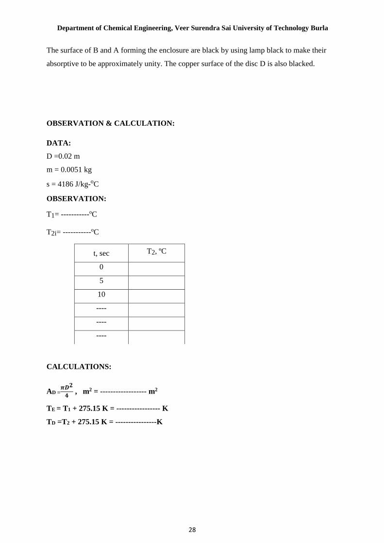
The surface of B and A forming the enclosure are black by using lamp black to make their

absorptive to be approximately unity. The copper surface of the disc D is also blacked.

OBSERVATION & CALCULATION:

DATA:

D =0.02 m

m = 0.0051 kg

s = 4186 J/kg-oC

OBSERVATION:

T1= -----------oC

T2i= -----------oC

CALCULATIONS:

AD =𝝅𝑫𝟐

𝟒 , m2 = ------------------ m2

TE = T1 + 275.15 K = ----------------- K

TD =T2 + 275.15 K = ----------------K

t, sec T2, ºC

0

5

10

----

----

----


29

Plot the graph of T vs t and obtain the slope dT/dt.

𝜎 =𝑚𝑠[

𝑑𝑇

𝑑𝑡]

𝐴𝐷(𝑇𝐸4−𝑇𝐷

4), Watt/m2K4

NOMENCLATURE:

AD = Area of disc, m2

D = Diameter of disc, m

m = Mass of disc, kg

s= Specific heat of the disc material, kJ/kg oC

T= Temperature of disc at time t, K

T1=Temperature of enclosure, oC

T2 =Temperature of disc at time t, oC

T2i =Initial temperature of the disc, oC

TE=Temperature of enclosure, K

TD =Initial temperature of the disc, K

t = Time, sec

σ=Stefan Boltzmann constant, Watt/m2k

4


1. Never run the apparatus if power supply is less than 180 volts and above than 230 volts.

2. Never switch ON mains power supply before ensuring that all the ON/OFF switches


t, sec TD =T2 + 275.15 K

0

5

10

----

----

----


30

3. Operator selector switches off temperature indicator gently.


TROUBLESHOOTING:

1. If electric panel is not showing the input on the mains light, check the main Supply.

REFERENCES:

1. Holman, J. P., “Heat Transfer”, 9th ed., McGraw Hill, ND, 2008, Page 372.

2. Y. A. Cengel, “Heat & Mass Transfer”, McGraw Hill, ND, 2008, Page 28, 667-671.


31

EXPERIMENT-7 & 8

OBJECTIVE: To study the heat transfer phenomena in parallel / counter flow arrangements.

AIM: To calculate overall heat transfer coefficient for both type of heat exchanger.

INTRODUCTION:

Heat Exchangers are devices in which heat is transferred from one fluid to another. The

necessity for doing this arises in a multitude of industrial applications. Common examples

of heat exchangers are the radiator of a car, the condenser at the back of a domestic

refrigerator and the steam boiler of a thermal power plant.

Heat Exchangers are classified in three categories:

1) Transfer Type.

2) Storage Type.

3) Direct Contact Type.

THEORY:

A transfer type of heat exchanger is one on which both fluids pass simultaneously through

the device and heat is transferred through separating walls. In practice most of the heat

exchangers used are transfer type ones.

The transfer type exchangers are further classified according to flow arrangement as -

1. Parallel flow in which fluids flow in the same direction.

2. Counter flow in which they flow in opposite direction and

3. Cross flow in which they flow at right angles to each other.

A simple example of transfer type of heat exchanger can be in the form of a tube type

arrangement in which one of the fluids is flowing through the inner tube and the other

through the annulus surroundings it. The heat transfer takes place across the walls of the


32

inner tube.

DESCRIPTION:

The apparatus consists of a tube in tube type concentric tube heat exchanger. The hot fluid

is hot water which is obtained from an insulated water bath using a magnetic drive pump

and it flows through the inner tube while the cold fluid is cold water flowing through the

annulus.

The hot water flows always in one direction and the flow rate of which is controlled by

means of a valve. The cold water can be admitted at one of the end enabling the heat

exchanger to run as a parallel flow apparatus or a counter flow apparatus. This is done by

valve operations.

RTDPT-100 type sensors measure the temperature. For flow measurement Rotameters are

provided at the inlet of hot and cold water supply. The readings are recorded when steady

state is reached.

UTILITIESREQUIRED:

Water supply 10 lit/min

(approx.) Drain.

Electricity Supply: 1 Phase, 220 V AC, 3 kW.

Floor area 2 m x 0.6m


1) Put water in bath and switch on the heaters.

2) Adjust the required temperature of hot water using DTC.

3) Adjust the valve. Allow hot water to recycle in bath by switching on the magnetic

pump.

4) Start the flow through annulus and run the exchanger either as parallel flow or counter


33

flow unit.

5) Adjust the flow rate on cold water side by rotameter provided.

6) Adjust the flow rate on hot water side by rotameter provided.

7) Keeping the flow rates same, wait till the steady state conditions are reached.

8) Record the temperatures on hot water and cold water side and the flow rates.

SPECIFICATIONS:

Inner Tube : Material = SS, ID = 9.5 mm, OD = 12.7 mm

Outer tube : Material = SS, ID = 28 mm, OD =

33.8mm Length of the heat Exchanger: L = 1.13m

Temperature Controller : Digital, Range:0-200oC

Temperature Indicator : Digital Range: 0-200oC & least count 0.1oC with

Multi-channel switch.

Temperature Sensors : RTD–PT-100 type. (5

Nos) Flow measurement : Rotameter (2No.)

Water Bath : Material: SS insulated with ceramic wool and powder

coated MS outer Shell fitted with heating elements.

Pump : FHP magnetic drive pump (Max operating temp.85

oC).

Heater : Nichrome wire, capacity 4kW

FORMULAE:

1. Rate of heat transfer from hot water,

Qh =Mh Cph (Thi-Tho), Watt

2. Rate of heat transfer to cold water,


34

Qc = M c C pc (Tco – Tci), Watt

3. Average heat transfer,

𝑄 =(𝑄ℎ+𝑄𝑐)

2, Watt

4. LMTD,

∆Tm =∆𝑇2−∆𝑇1

𝑙𝑛∆𝑇2∆𝑇1

, °C

where: ∆T1=Thi – Tci (for parallel flow)

=Thi – Tco (for counter flow)

and ∆T2=Tho – Tco (for parallel flow)

=Tho – Tci (for counter flow)

Note that in a special case of Counter Flow Exchanger exists when the heat capacity

rates Cc & Ch are equal, then Thi – Tco = Tho – Tci thereby making ∆Ti = ∆To. In

this case LMTD is of the form 0/0 and so undefined. But it is obvious that since ∆T is

constant throughout the exchanger, hence

∆Tm=∆Ti = ∆To

(acc. to ref. Fundamental of Engineering Heat & Mass Transfer by R.C. Sachdeva, Pg.

499)

Overall heat transfer coefficient,

Ui =Q

Ai∆Tm, Watt/m2°C & Uo =

Q

Ao∆Tm, Watt/m2°C

OBSERVATION & CALCULATION:

DATA:

Inside heat transfer area, Ai = 7.088* 10-5 m2


35

Outside heat transfer area, A0 = 61.575*10-5 m2

OBSERVTION TABLE:

FOR PARALLEL FLOW:

Sl. No. Hot water side Cold water side

Flow rate Thi °C Tho °C Flow rate Tci °C Tco°C

1

2

FOR COUNTER FLOW:

Sl. No. Hot water side Cold water side

Flow rate Thi °C Tho °C Flow rate Tci °C Tco°C

1

2

CALCULATIONS:

CASE I: Counter Flow

Mass flow rate of hot water:

Average temperature =------------°C

MH = -----Kg/hr

ρH = -------Kg/m3

CpH=-------J/Kg°K

Mass flow rate of cold water


MC = -----Kg/hr

ΡC = -------Kg/m3


36

CpC=-------J/Kg°K

Heat flow Rate

Qh= Mh × Cph × ΔT=--------W

Qc= Mc × Cpc × ΔT=--------W

Effectiveness of HE, ε = 𝑄𝑎𝑐𝑡𝑢𝑎𝑙

𝑄𝑚𝑎𝑥× 100 %

𝑄𝑎𝑐𝑡𝑢𝑎𝑙 =𝑄𝐶+𝑄𝐻

2 = -----------KW

Q max = Mh Cph (Thi- Tci) =-------KW

LMTD for counter flow = (Thi−Tco)−(Tho−Tci)

ln [Thi−TcoTho−Tci

]

𝑈𝑜 =𝑄

𝐴𝑜×𝐿𝑀𝑇𝐷 =------------W/m2°C

𝑈𝑖 =𝑄

𝐴𝑖×𝐿𝑀𝑇𝐷=------------- W/m2°C

CASE II: Parallel Flow

Mass flow rate of hot water:


MH = -----Kg/hr

ρH = -------Kg/m3

CpH=-------J/Kg°K

Mass flow rate of cold water


MC = -----Kg/hr

ΡC = -------Kg/m3

CpC=-------J/Kg°K


37

Heat flow Rate

Qh= Mh × Cph × ΔT=--------W

Qc= Mc × Cpc × ΔT=--------W

Effectiveness of HE, ε = 𝑄𝑎𝑐𝑡𝑢𝑎𝑙

𝑄𝑚𝑎𝑥× 100 %

𝑄𝑎𝑐𝑡𝑢𝑎𝑙 =𝑄𝐶+𝑄𝐻

2 = -----------KW

Q max = Mh Cph (Thi- Tci) =-------KW

LMTD for parallel flow = (Thi−Tci)−(Tho−Tco)

ln [Thi−Tci

Tho−Tc0]

𝑈𝑜 =𝑄

𝐴𝑜×𝐿𝑀𝑇𝐷 =------------W/m2°C

𝑈𝑖 =𝑄

𝐴𝑖×𝐿𝑀𝑇𝐷=------------- W/m2°C

NOMENCLATURE:

Qh = heat loss by the hot water, W

Mh = mass flow rate of the hot water

Cph = specific heat of hot fluid at mean temperature

Tho = outlet temperature of the hot water

Thi = inlet temperature of the hot water

Qc = heat gained by the cold water

Mc = mass flow rate of the cold water

Cpc = specific heat of cold fluid at mean temperature

Tco = outlet temperature of the cold water

Tci = inlet temperature of the cold water

Q = average heat transfers from the system

U = overall heat transfer coefficient

Ui = Inside overall heat transfer coefficient

Ai = πri X-sectional area of inner pipe


38

Uo = outside overall heat transfer coefficient

Ao = πri X-sectional area of outer pipe

PRECAUTIONS AND MAINTENANCEINSTRUCTION:




3. Never run the apparatus if power supply is less than 180 volts and above than 230volts.



6. Don’t switch ON the heater before filling the water into the bath.

TROUBLESHOOTING:

1. If electric panel is not showing the input on the mains light. Check the fuse and

also check the main supply.

2. If D.T.I displays “1” on the screen check the computer socket if loose tight it.

3. If temperature of any sensor is not displays in D.T.I check the connection and rectify that.

REFERENCES:

1. Holman, J.P., “Heat Transfer”, 8th ed., McGraw Hill, NY, 1976.


3. McCabe, W.L., Smith, J.C., Harriott, P., “Unit Operations of Chemical

engineering”, 4th ed. McGraw Hill, NY, 1985.


39

4. Coulson, J.M., Richardson, J.F., “Coulson & Richardson’s Chemical Engineering Vol.

-1”, 5th ed., Asian Books ltd., ND, 1996.


40

EXPERIMENT-9 & 10

OBJECTIVE: To study of heat transfer in the process of condensation.

AIM: To find the heat transfer co-efficient for Drop-wise condensation and Film-wise

condensation process.

INTRODUCTION:

In all applications, the steam must be condensed as it transfers heat to a cooling medium,

e.g. cold water in the condenser of a generating station, hot water in a heating calorimeter,

sugar refinery, etc. During condensation very high heat fluxes are possible &provided the

heat can be quickly transferred from the condensing surface to the cooling medium, heat

exchangers using steam can be compact & effective.

THEORY:

Steam may condense on to a surface in two distinct modes, known as “Film wise” & “Drop

wise”. For the same temperature difference between the steam & the surface, drop wise

condensation is much more effective than film wise & for this reason the former is desirable

although in practical plants, it rarely occurs for prolonged periods.

FILMWISE CONDENSATION:

Unless specially treated, most materials are wettable & as condensation occur a film

condensate spreads over the surface. The thickness of the film depends upon a numbers of

factors, e.g. the rate of condensation, the viscosity of the condensate and whether the surface

is vertical or horizontal, etc. Fresh vapor condenses on to the outside of the film & heat is

transferred by conduction through the film to the metal surface beneath. As the film

thickness it flows downward &drips from the low points leaving the film intact & at an

equilibrium thickness.

The film of liquid is a barrier to the transfer of heat and its resistance accounts for most of

the difference between the effectiveness of film wise and drops wise condensation.

DROPWISE CONDENSATION:

By specially treating the condensing surface the contact angle can be changed and the surface

becomes ‘non-wettable’. As the steam condenses, a large number of generally spherical beads


41

cover the surface. As condensation proceeds, the beads become larger, coalesce, and then

strike downwards over the surface. The moving bead gathers all the static beads along its

downward in its trail. The ‘bare’ surface offers very little resistance to the transfer of heat and

very high heat fluxes are therefore possible. Unfortunately, due to the nature of the material

used in the construction of condensing heat exchangers, film wise condensation is normal.

(Although many bare metal surfaces are ‘non- wettable’ this is not true of the oxide film

which quickly covers the bare material)

DESCRIPTION:

The equipment consists of a metallic container in which steam generation takes place. The

lower portion houses suitable electric heater for steam generation. A special arrangement is

provided for the container for filling the water. The glass cylinder houses two water cooled

copper condensers, one of which is chromium plated to promote drop wise condensation and

the other is in its natural state to give film wise condensation. A connection for pressure gauge

is provided. Separate connections of two condensers for passing water are provided. One Rota

meter with appropriate piping can be used for measuring water flow rate in one of the

condensers under test. A digital temperature indicator provided has multipoint connections,

which measures temperatures of steam, two condensers, water inlet & outlet temperature of

condenser water flows.

UTILITIES REQUIRED:

Water supply 5 lit/min (approx.)

Electricity Supply: 1 Phase, 220 V AC, and 2.0 kW.

Table for set-up support (optional)


1. Fill water in steam generator through funnel by opening the valve.

2. Fill water in the steam generator up to half mark. (Visible in transparent glass

window).

3. Start water flow through one of the condensers, which is to be tested and note down

water flow rate in rotameter. Ensure that during measurement, water is flowing only

through the condenser under test and second valve is closed.


42

4. When the temperature of steam reaches the set point, start the steam supply to

condenser under test. Steam gets condensed on the tubes, and falls down in the

cylinder.

5. Depending upon type of condenser under test Drop wise or Film wise can be

visualized.

6. If the water flow rate is low, then steam pressure in the chamber will rise and pressure

gauge will read the pressure. If the water flow rate is matched, then condensation will

occur at more or less atmospheric pressure or up to 1 kg pressure.

7. Observations like temperatures, water flow rates, and pressure are noted down in the

observations table at the end of each set.

Repeat above steps to test second condenser.

8. SPECIFICATION:

Condensers = One chromium plated for drop wise condensation & one natural finish for Film

wise condensation otherwise identical in construction.

Dimensions = 19 mm outer dia. 160 mm length, Fabricated from copper with reverse flow in

Concentric tubes. Fitted with Temperature sensor for surface temperature measurement

Main Unit= M.S. Fabricated construction comprising test section & steam generation section.

Test section provided with glass cylinder for visualization of the process.

Heating Elements = Suitable water heater.

Instrumentation = 1) Temperature Indicator: Digital 0-199.9°C & least count 0.1°C with

Multi-channel switch.

2) Temperature Sensors: RTD PT-100 Type.

3) Rotameter: for measuring water flow rate.

4) Pressure Gauge: Dial type 0 - 2 Kg/cm2

FORMULAE:

Heat losses from steam, Qs = Ms * , Watt


43

Heat taken by cold water, Qw Mw *Cp*(T5 T4), Watt

Average hear transfer, Q =(𝑄𝑠+𝑄𝑤)

2, Watt

Inside heat transfer co-efficient, hi =Q

(Ai∗Tm), Watt/m2 -OC

Outside heat transfer co-efficient, ho= Q

Ao∗∆Tm , Watt/m2-OC

∆𝑇𝑚 =∆𝑇2 − ∆𝑇1

𝑙𝑛 (∆𝑇2

∆𝑇1)

∆𝑇2 = 𝑇3 − 𝑇2 (For Plain Condenser)

∆𝑇1 = 𝑇3 − 𝑇1 (For Plated Condenser)

Experimental overall heat transfer co-efficient,

1

𝑈𝐸𝑋=

1

ℎ1+ [

𝐷𝑖

𝐷𝑜𝑥

1

ℎ𝑜]

Reynolds Number,

𝑅𝑒𝑑 =4𝑚𝑤

𝜋𝐷𝑖𝜌1𝑣1

Nusselt Number,

Nu1 = 0.023(Red)0.8(Pr)

Inside heat transfer co-efficient,

hi = Nu1K

LW/m2 oc

Outside heat transfer coefficient,

ho = 0.943[ρ2

2gk23

(Ts−Tw)μL]

0.25

,Watt/m2-OC

Theoretical overall heat transfer coefficient,

1

𝑈𝑇𝐻=

1

ℎ𝑖+[

𝐷𝑖

𝐷𝑜 𝑥

1

ℎ𝑜]


44

OBSERVATIONS & CALCULATIONS:

DATA:

O.D of heat transfer surface, Do= 19mm

I.D. of heat transfer surface, Di =16mm

Length of heat transfer surface, L = 160mm

Inside heat transfer area, Ai = 0.000201 m2

Outside heat transfer area, Ao= 0.000284 m2

Latent heat of steam, λ = 2257.2 x 103 J/kg

OBSERVATION TABLE:

Condenser under Test:

Sl.

No.

Water Flow Rate

(LPH)

Steam

Condensed (ml)

Time

(min)

Temperature

T1 T2 T3 T4 T5

TEMPERATURE:

T1- Surface Temperature of Plated Condenser

T2- Surface Temperature of Plain Condenser

T3- Temperature of steam in column

T4- Water inlet temperature (common for both condensers)

T5- Water outlet temperature (common for both condensers)


45

CALCULATION:

Properties of water at bulk mean temperature of water i.e. (Twi +Two)/2 Where Twi and Two

are water inlet & outlet temperatures.

Following properties are required:

CP = Specific heat of water (4.186 kJ/kg- K)

1 = Density of water kg/m3



1 = Kinematics Viscosity at 40 0C (0.657 m2/sec)

2 = Kinematics Viscosity at 100 0C (0.2932 m2/sec)

μ = Viscosity of water at 100 ℃ (1.154)

μ = Viscosity of water at 35 ℃ (1.215)

k1 = Thermal conductivity at 40 ℃ (540W /m -K)

k2 =Thermal conductivity at 100 ℃ (586W /m -K)

Now calculate,

Reynolds’s number,

𝑅𝑒𝑑 =4𝑚𝑤

𝜋𝐷𝑖𝜌1𝑣1

and, Prandtl Number,

𝑃𝑟 =𝜇𝐶𝑝

𝐾

Nusselt Number,

Nu = 0.023 (Red)0.8 (Pr)0.4

h1 =𝑁𝑢1𝐾

𝐿𝑊/m2-oc


46

Now calculate heat transfer coefficient on outer surface of the condenser (ho). For this

properties of water are taken at bulk mean temperature of condensate i.e

𝑻𝒔+𝑻𝒘

𝟐 ℃ =T2

oC

Properties needed are:

2 =Density of water Kgm/m3

K2 = Thermal Conductivity Kcal/ hr - mC (W/ m C)

= Viscosity of condensate Kgf - sec/m2. (Kg/m sec)

=Heat of evaporation J/Kg. (2257.2 x 103 J/kg)

ho = 0.943[2

2gk23

(Ts−Tw)μL]

0.25

From these values overall Heat Transfer coefficient (U) can be calculated.

1

𝑈 =

1

ℎ𝑖 + [

𝐷𝑖

𝐷𝑜 𝑥

1

ℎ𝑜] Kcal/hr-m2-oC

And,

Calculate the experimental overall heat transfer co-efficient and compare with theoretical

overall heat transfer coefficient. Same procedure can be repeated for other condenser. Except

for some exceptional cases overall heat transfer co-efficient for Drop-wise Condensation will

be higher than that of film wise condensation. Results may vary from theory in some degree

due to unavoidable heat losses.

NOMENCLATURE:

Did = Inner dia. of condenser.

Dod = outer dia. of condenser

hi = Inside Heat Transfer Co-efficient.

ho= outside Heat Transfer Co-efficient.

TS = Temperature of steam C.


47

TW = Temperature of condenser wall C.

∆Tm = Log mean temperature difference

Ms = Rate of steam condensation, Kg/s

Mw = Cold water flow rate, Kg/s

Cp = Specific heat of water.

G = Acceleration due to gravity

L = Length of condenser

= Density of water kg/m3

= Kinematics Viscosity m2/sec.

k = Thermal conductivity, W/m-OC

Pr= Prandtl number.

PRECAUTIONS & MAINTENANCE INS

1. Use the stabilized A.C. Single Phase supply only.



3. Voltage to heater starts and increases slowly.


5. Never run the apparatus if power supply is less than 180 volts and above than 240 volts.


7. Do not start heater supply unless water is filled in the test unit.

8. Always keep the apparatus free from dust. There is a possibility of getting abrupt result

if the supply voltage is fluctuating or if the satisfactory steady state condition is not

reached.

TROUBLE SHOOTING:

1. If electric panel is not showing the input on the mains light. Check the fuse and also

check the Main supply.


48

2. If D.T.I displays “1” on the screen check the computer socket if loose tight it.

3. If temperature of any sensor is not displays in D.T.I check the connection and rectify

that.

REFERENCES:

1. Holman, J.P., “Heat Transfer”, 8th ed., McGraw Hill, NY, 1976.


3. Perry, R.H., Green, D. (editors), “Perry’s Chemical Engineers’ Handbook”, 6th

ed., McGraw Hill, NY, 1985.

4. Coulson, J.M., Richardson, J.F., “Coulson & Richardson’s Chemical Engineering

Vol. - 6”, 5th ed., Asian Books ltd., ND, 1996.

heat transfer laboratory lab manual list of …

Documents