heating systems in buildings - method for calculation of ... · pdf fileheating systems in...

Document type: European Standard Document subtype: Document stage: Formal Vote Document language: E

Doc. CEN/TC 228 N553 CEN/TC 228

Date: 2006-08

CEN/TC 228 WI 030

CEN/TC 228

Secretariat: DS

Heating systems in buildings - Method for calculation of system energy requirements and system efficiencies - Part 2-3: Space heating distribution systems Einführendes Element — Haupt-Element — Teil 2-3: Ergänzendes Element

Systèmes de chauffage dans les bâtiments — Élément central — Partie 2-3 : Élément complémentaire

ICS:

Descriptors:

prEN 15316-2-3:2006 (E)

2

Contents Page

Foreword..............................................................................................................................................................3 Introduction .........................................................................................................................................................4 1 Scope ......................................................................................................................................................5 2 Normative references ............................................................................................................................5 3 Symbols, units and indices ..................................................................................................................5 4 Principle of the method and definitions ..............................................................................................7 5 Electrical energy demand – Auxiliary energy demand ......................................................................8 5.1 General....................................................................................................................................................8 5.2 Design Hydraulic power........................................................................................................................8 5.3 Detailed Calculation Method.................................................................................................................9 5.3.1 Input- / Output data................................................................................................................................9 5.3.2 Calculation Method............................................................................................................................. 10 5.3.3 Correction factors............................................................................................................................... 11 5.3.4 Expenditure energy factor ................................................................................................................. 13 5.3.5 Intermittent operation......................................................................................................................... 17 5.4 Deviations from the detailed calculation method............................................................................ 20 5.5 Monthly energy demand .................................................................................................................... 20 5.6 Recoverable auxiliary energy............................................................................................................ 21 6 Heat emission of distribution systems............................................................................................. 21 6.1 General................................................................................................................................................. 21 6.2 Detailed Calculation Method.............................................................................................................. 21 6.2.1 Input- / Output data............................................................................................................................. 21 6.2.2 Calculation method ............................................................................................................................ 21 6.2.3 Heat emission of accessories ........................................................................................................... 23 6.2.4 Recoverable and non-recoverable heat emission........................................................................... 23 6.2.5 Total heat emission ............................................................................................................................ 23 6.3 Calculation of linear thermal transmittance (W/mK):...................................................................... 23 7 Calculation of mean part load of distribution per zone .................................................................. 24 8 Calculation of supply and return temperature depending on mean part load of distribution.... 25 Annex A (informative) Preferred procedures ................................................................................................ 26 A.1 Simplified Calculation Method of annual electrical auxiliary energy demand ............................. 26 A.1.1 Input- / Output data............................................................................................................................. 26 A.1.2 Calculation method ............................................................................................................................ 27 A.1.3 Correction factors............................................................................................................................... 28 A.1.4 Expenditure energy factor ................................................................................................................. 29 A.1.5 Intermittent operation......................................................................................................................... 30 A.2 Tabulated calculation method of annual electrical auxiliary energy demand.............................. 30 A.2.1 Tabulated calculation of annual electrical auxiliary energy demand............................................ 30 A.3 Simplified Calculation Method of heat emission............................................................................. 32 A.3.1 Input- / Output data............................................................................................................................. 32 A.3.2 Approximation of the length of pipes per zone in distribution systems ...................................... 33 A.3.3 Approximation of U-Values................................................................................................................ 34 A.3.4 Equivalent length of valves ............................................................................................................... 34 A.4 Tabulated Calculation Method of annual heat emission ................................................................ 35 A.5 Tabulated calculation of annual heat emission............................................................................... 35 A.6 Example ............................................................................................................................................... 36

prEN 15316-2-3:2006 (E)

3

Foreword

This document (prEN 15316-2-3:2005) has been prepared by Technical Committee CEN/TC 228 “Heating systems in buildings”, the secretariat of which is held by DS.

The subjects covered by CEN/TC 228 are the following:

- design of heating systems (water based, electrical etc.);

- installation of heating systems;

- commissioning of heating systems;

- instructions for operation, maintenance and use of heating systems;

- methods for calculation of the design heat loss and heat loads;

- methods for calculation of the energy performance of heating systems.

Heating systems also include the effect of attached systems such as hot water production systems.

All these standards are systems standards, i.e. they are based on requirements addressed to the system as a whole and not dealing with requirements to the products within the system.

Where possible, reference is made to other European or International Standards, a.o. product standards. However, use of products complying with relevant product standards is no guarantee of compliance with the system requirements.

The requirements are mainly expressed as functional requirements, i.e. requirements dealing with the function of the system and not specifying shape, material, dimensions or the like.

The guidelines describe ways to meet the requirements, but other ways to fulfil the functional requirements might be used if fulfilment can be proved.

Heating systems differ among the member countries due to climate, traditions and national regulations. In some cases requirements are given as classes so national or individual needs may be accommodated.

In cases where the standards contradict with national regulations, the latter should be followed.

prEN 15316-2-3:2006 (E)

4

Introduction

In a distribution system, energy is transported by a fluid from the heat generation to the heat emission. As the distribution system is not adiabatic, part of the energy carried is emitted to the surrounding environment. Energy is also required to distribute the heat carrier fluid within the distribution system. In most cases this is electrical energy required by the circulation pumps. This leads to additional thermal and electrical energy demand.

The thermal energy emitted by the distribution system and the electrical energy required for the distribution may be recovered as heat if the distribution system is placed inside the heated envelope of the building.

This standard provides three methods of calculation.

The detailed calculation method describes the basics and the physical background of the general calculation method. The required input data are part of the detailed project data assumed to be available (such as length of pipes, type of insulation, manufacturer's data for the pumps, etc.). The detailed calculation method provides the most accurate energy demand and heat emission.

For the simplified calculation method, some assumptions are made for the most relevant cases, reducing the required input data (e.g. the length of pipes are calculated by approximations depending on the outer dimensions of the building and efficiency of pumps are approximated). This method may be applied if only few data are available (in general at an early stage of design). With the simplified calculation method, the calculated energy demand is generally higher than the calculated energy demand by the detailed calculation method. The assumptions for the simplified method depend on national designs. Therefore this method is part of Annex A.

The tabulated calculation method is based on the simplified calculation method with some further assumptions being made. Only input data for the most important influences are required with this method. The further assumptions depend on national design also. Therefore the tabulated method is part of Annex A also.

Other influences, which are not reflected by the tabulated values, shall be calculated by the simplified or the detailed calculation method. The energy demand determined from the tabulated calculation method is generally higher than the calculated energy demand by the simplified calculation method. Use of this method is possible with a minimum of input data.

The general calculation method for the electrical energy demand of pumps consists of two parts. The first part is calculation of the hydraulic demand of the distribution system and the second part is calculation of the expenditure energy factor of the pump. Here, it is possible to combine the detailed and the simplified calculation method. For example, calculation of pressure loss und flow may be done by the detailed calculation method and calculation of the expenditure energy factor may be done by the simplified calculation method (when the data of the building are available and the data of the pump are not available) or vice versa.

In national annexes, the simplified calculation method as well as the tabulated calculation method could be applied through a. o. relevant boundary conditions of each country, thus facilitating easy calculations and quick results. In national annexes it is only allowed to change the boundary conditions. The calculation methods must be used as described. The recoverable energy of the auxiliary energy demand is given as a fixed ratio and is therefore also easy to determine.

prEN 15316-2-3:2006 (E)

5

1 Scope

This standard provides a methodology to calculate/estimate the heat emission of water based distribution systems for heating and the auxiliary energy demand, as well as the recoverable energy. The actual recovered energy depends on the gain to loss ratio. Different levels of accuracy corresponding to the needs of the user and the input data available at each design stage of the project are defined in the standard. The general method of calculation can be applied for any time-step (hour, day, month or year).

Pipework lengths for the heating of decentralised non-domestic ventilation systems equipment are to be calculated in the same way as for water based heating systems. For central non-domestic ventilation systems equipment the length is to be specified in accordance with its location.

NOTE: It is possible to calculate the heat emission and auxiliary energy demand for cooling systems with the same calculation methods as shown in this standard. Specifically, determination of auxiliary energy demand is based on the same assumtions for efficiency of pumps, because the standard curve is an approximation for inline and external motors. It has to be decided by the standardisation group of CEN if the extension for cooling systems should be made in this standard. This is also valid for distribution systems in HVAC (in ducts) and also for special liquids.

2 Normative references

The following referenced documents are indispensable for the application of this document. For dated references, only the edition cited applies. For undated references, the latest edition of the referenced document (including any amendments) applies.

EN 12831, Heating systems in buildings - Method for calculation of the design heat load

EN ISO 13790, Thermal performance of buildings - Calculation of building energy demand for heating (ISO 13790: 2004)

3 Symbols, units and indices

For the purposes of this standard, the symbols, units and indices given in Table 1 apply.

Table 1 — Symbols, units and indices

A Heated floor in the zone [m²] B Building width [m]

Pc Specific heat capacity [kJ/kg K]

ede , Expenditure energy factor for operation of circulation pump [-]

Sf Correction factor for supply flow temperature control [-]

NETf Correction factor for hydraulic networks (layout) [-]

SDf Correction factor for heating surface disign [-]

HBf Correction factor for hydraulic balance [-]

PMGf , Correction factor for generators with integrated pump management [-]

PLf Correction factor for partial load characteristics [-]

Cf Correction factor for control of the pump [-]

PSPf Correction factor for selection of design point [-]

ϑf Correction factor for differential temperature dimensioning [-]

prEN 15316-2-3:2006 (E)

6

qf & Correction factor for surface related heating load [-]

ηf Correction factor for efficiency [-]

L Building length [m]

maxL Maximum length of pipe [m] m ratio of flow over the heat emitter to flow in the ring [-] n exponent of the emission system [-]

Gn Number of floors [-]

pΔ Differential pressure at design point [kPa]

HSpΔ Differential pressure of heating surfaces [kPa]

CVpΔ Differential pressure of control valves for heating surfaces [kPa]

ZVpΔ Differential pressure of zone valves [kPa]

GpΔ Differential pressure of heating supply [kPa]

FHpΔ Differential pressure of floor heating systems [kPa]

ADDpΔ Differential pressure of additional resistances [kPa]

hydrP Hydraulic power at design point [W]

PumpP Actual power input [W]

refPumpP , Reference power input [W]

NQ& design heating load [kW]

wrdQ ,, Recoverable energy into heating water [kWh/timstep]

ardQ ,, Recoverable energy into surrounding air [kWh/timstep]

R Pressure loss in pipes [kPa/m]

Ht Heating hours per year [h/year]

LU linear thermal transmittance [W/mK]

V& Flow in design point [m³/h] minV& minimum volume flow [m³/h]

edW , Electrical energy demand [kWh/year]

edW ,′′ Electrical energy demand (tabulated) [kWh/year]

MedW ,, Monthly total electrical energy demand [kWh/month]

hydrdW , Hydraulic energy demand [kWh/year] z Resistance ratio of components [-] α time factor [-]

setbα set back time factor [-]

HKϑΔ Dimensioned heating system temperature difference [K]

Pη Efficiency of pump at design point [-]

Dβ Mean part load of the distribution [-] ρ Specific density [kg/m³]

iϑ surrounding temperature [° C]

mϑ mean medium temperature [° C]

uϑ temperature in unheated space [° C]

prEN 15316-2-3:2006 (E)

7

sϑ supply temperature [° C]

rϑ return temperature [° C]

saϑ design supply temperature [° C]

raϑ design return temperature [° C]

4 Principle of the method and definitions

The method allows the calculation of the heat emission and the auxiliary energy demand of water based distribution systems for heating circuits (primary and secondary) as well as the recoverable energy. As shown in Figure 1 a heating system can divided in three parts – emission and control, distribution and generation. An easy heating system has no buffer-storage and no distributor/collector and also only one pump. Larger heating systems have more then one heating circuits with different emitters as so called secondary heating circuits. Mostly such heating systems have also more than one heat generator (individual or equal) with so called primary heating circuits (in figure 1 only one primary circuit is shown). The subdivision in primary and secondary circuits is given by any hydraulic separator which can be a buffer-storage with a large volume or a hydraulic separator with a small volume. Anyhow the calculation method is valid for a closed heating circuit and therefore the equations have to used for each circuit taking into account the corresponding values.

Figure 0 - Scheme distribution and definitions of heating circuits

prEN 15316-2-3:2006 (E)

8

Key

1 Next heating circuit 2 pump 3 room 4 emission 5 buffer-storage 6 pump 7 generator 8 generation 9 distribution 10 primary heating circuits 11 secondary heating circuits

Controls in distribution systems are thermostatic valves at the emitter which throttles the flow or room thermostats which shut on/off the pump. Only if the flow is throttled the control of the pump (speed control) is valid.

5 Electrical energy demand – Auxiliary energy demand

5.1 General

The auxiliary energy demand of hydraulic networks depends on the distributed flow, the pressure drop and the operation condition of the pump. While the design flow and pressure drop is important for determining the pump size, the part load factor determines the energy demand in a time step. The hydraulic power at the design point can be calculated from physical basics. However, for calculation of the hydraulic power during operation, this can only be achieved by a simulation. Therefore, for the detailed calculation method in this standard correction factors are applied, which represent the most important influences on auxiliary energy demand, such as part load, controls, design criteria, etc. The general calculation approach is to separate the hydraulic demand, which depends on the design of the network, and the expenditure energy for operation of the pump, which take into account the efficiency of the pump in general. However, for calculation of the expenditure energy during operation, the knowledge of the efficiency of the pump at each operation point is required, Therefore, for the detailed calculation method in this standard correction factors are applied also, which represent the most important influences an expenditure energy, such as efficiency, part load, design point selection and control.

All the calculations are made for a zone of the building with the affiliated area, length, width, height and levels.

5.2 Design Hydraulic power

For all the calculations, the hydraulic power and the differential pressure of the distribution system at the design point are important. The hydraulic power is given by:

VpPhydr&⋅Δ⋅= 2778,0 [W] (1)

where:

V& Flow at design point [m³/h] pΔ Differential pressure at design point [kPa]

prEN 15316-2-3:2006 (E)

9

The flow is calculated from the heat load NQ& of the zone (design heat load according to EN 12831) and the

design temperature difference HKϑΔ of the heating system

HKP

N

cQ

VϑΔ⋅ρ⋅

⋅=

&& 3600

[m³/h] (2)

where:

Pc Specific heat capacity [kJ/kg K] ρ Density [kg/m³]

HKϑΔ Design temperature difference [K]

The differential pressure for a zone at the design point is determined by the resistance in the pipes (including components) and the additional resistances (the most important are listed below):

( ) ADDGZVCVHS pppppLRzp Δ+Δ+Δ+Δ+Δ+⋅⋅+=Δ max1 [kPa] (3)

where:

z Resistance ratio of components [-] R Pressure loss per m [kPa/m]

maxL Maximum pipe length of the heating circuit [m]

HSpΔ Differential pressure of heating surface [kPa]

CVpΔ Differential pressure of control valve for heating surface [kPa]

ZVpΔ Differential pressure of zone valves [kPa]

GpΔ Differential pressure of heat supply [kPa]

ADDpΔ Differential pressure of additional resistances [kPa]

5.3 Detailed Calculation Method

5.3.1 Input- / Output data

The input data for the detailed calculation method are listed below. These are all part of the detailed project data.

hydrP Hydraulic power at the design point for the zone [in W], calculated by the knowledge of

NQ& Design heat load of the zone according to EN 12831

HKϑΔ Design temperature difference for the distribution system in the zone [K]

maxL Maximum pipe length of the heating circuit in the zone [m]

pΔ Differential pressure of the circuit in the zone [kPa]

Dβ Mean part load of the distribution [-]



NETf Correction factor for hydraulic networks [-]

prEN 15316-2-3:2006 (E)

10

SDf Correction factor for heating surface dimensioning [-]

HBf Correction factor for hydraulic balance [-] Pump control

ede , Expenditure energy factor for operation of the circulation pump [-], calculated by this standard, using:


PLf Correction factor for part load [-]

PSPf Correction factor for design point selection [-]

Cf Correction factor for control of the pump [-] Design temperature level

emitter type

Intermittent operation

The output data are:

edW , Total electrical energy demand [kWh/year]


wrdQ ,, Recoverable energy to the water [kWh/timstep]

ardQ ,, Recoverable energy to the surrounding air [kWh/timstep]

5.3.2 Calculation Method

The electrical energy demand for circulation pumps for water based heating systems is calculated by:

edhydrded eWW ,,, ⋅= (4)

where

edW , Electrical energy demand [kWh/year]

hydrdW , Hydraulic energy demand [kWh/year]

ede , Expenditure energy factor for operation of circulation pump [-]

The hydraulic energy demand for the circulation pumps in heating systems is determined from the hydraulic power at the design point ( hydrP ), the mean part load of the distribution ( Dβ ) and the heating hours in the time

step ( Ht ):

PMGHBSDNETSHDhydr

hydrd ffffftP

W ,, 1000⋅⋅⋅⋅⋅⋅⋅= β (kWh/year) (5)

where:

hydrP Hydraulic power at design point [W]

prEN 15316-2-3:2006 (E)

11

Dβ Mean part load of the distribution [-]




SDf Correction factor for heating surface dimensioning [-]

HBf Correction factor for hydraulic balance [-]

PMGf , Correction factor for generators with integrated pump management [-]

The correction factors, Sf , NETf and SDf include the most important parameters related to dimensioning of

the heating system. The factor HBf take into account the hydraulic balance of the distribution system. The

correction factor PMGf , for generators with integrated pump management take into account the reduction of operation time in relation to the heating time.

5.3.3 Correction factors

The correction factors are based on a wide range of simulations of different networks. Some of the correction

factors can not changed without changing the method. Correction factors which are based on assumptions

can be changed on national requirements (see Annex A.1.3).

5.3.3.1 Correction factor for supply flow temperature control Sf

1=Sf for systems with outdoor temperature compensation

Sf see Figure 1, for systems without outdoor temperature compensation (i.e. constant flow tempera-ture) or very much higher flow temperature than necessary

prEN 15316-2-3:2006 (E)

12

Key

1 Correction factor Sf [-] 2 Ground plan AN [m²] 3 Flow temperature characteristics

Figure 1 — Correction factor Sf for constant flow temperature and very much higher flow temperature

5.3.3.2 Correction factor for hydraulic networks NETf

1=NETf for a two-pipe ring line horizontal layout (on each floor)

NETf see Table 2 for other types of layout

Table 2 — Correction factors for hydraulic network

Network design One family house Dwellings

2 – pipe system Ring line 1,0 1,0 Ascending – pipe 0,93 0,92 Star-shaped 0,98 0,98

The star-shaped network design is also valid for floor heating systems.

prEN 15316-2-3:2006 (E)

13

For one-pipe heating systems, the correction factor NETf is given by

7,06,8 +⋅= mfNET (6) where:

m ratio of flow over the heat emitter to flow in the ring [-]

5.3.3.3 Correction factor for heating surface dimensioning SDf

1=SDf for dimensioning according to design heat load

96,0=SDf in case of additional over-sizing of the heating surfaces

5.3.3.4 Correction factor for hydraulic balance HBf

See Annex A.1.3

5.3.3.5 Correction factor for generators with integrated pump management PMGf ,

See Annex A.1.3 5.3.4 Expenditure energy factor

For assessment of partial load conditions and control performance of the circulation pump, the expenditure energy factor is determined by:

CPSPPLed ffffe ⋅⋅⋅= η, (7)

where


PLf Correction factor for part load [-]

PSPf Correction factor for design point selection [-]

Cf Correction factor for control [-]

With these four correction factors, the expenditure energy factor take into account the most important influences on the energy demand, representing the design, the efficiency of the pump, the part load and the control.

The physical relations are shown in Figure 2.

prEN 15316-2-3:2006 (E)

14

Key

1 Pressure Head H [m] 2 Power P1 [W]

3 Flow rate [m³/h] 4 H0,max

5 Hpump 6 HAusl 7 HPL 8 Phydr

9 PPL 10 Ppump

11 Ppump,max 12 PPL,C

prEN 15316-2-3:2006 (E)

15

13 Ppump,ref

14 PLV& 15 V&

16 PL

CPLPL P

Pf ,= 17

refpump

pumpPSP P

Pf

,

=

18 hydr

refpump

PP

f ,=η 19 pumpD

PLPL P

Pf⋅

=β

Figure 2 — Expenditure energy - physical interpretation of the correction factors

5.3.4.1 Correction factor for efficiency ηf

The correction factor for efficiency is given by the relation between the reference power input at the design point and the hydraulic power at the design point.

hydr

ref Pump

PP

f ,=η (8)

The reference power input is calculated by means of the pump characteristic line:

⎟⎟

⎠

⎞

⎜⎜

⎝

⎛

⎟⎟⎠

⎞⎜⎜⎝

⎛+⋅=

5,0

,20025,1

hydrhydrrefPump P

PP (9)

5.3.4.2 Correction factor for part load PLf

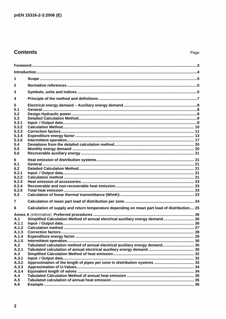
The correction factor for part load take into account the reduction of pump efficiency by partial load. It also take into account the hydraulic characteristics of non-controlled pumps. The impact of the partial load on the pipe system, and thus on the hydraulic energy demand, is taken into account by the mean part load of the distribution Dβ , according to 5.3.2.

Figure 3 shows the correction factor for part load of the pump depending on the mean part load of the distribution.

prEN 15316-2-3:2006 (E)

16

Key

12 Correction factor fPL [-] 13 Mean part load of distribution ßD 14 Mean part load Ratio (PLR)

Figure 3 — Correction factor for part load of the pump

5.3.4.3 Correction factor for design point selection PSPf

The correction factor for design point selection PSPf is given by the relation between the actual power input of the pump and the reference power input at the design point:

refPump

PumpPSP P

Pf

,

= (10)

where

PumpP actual power input of pump at design point [W]

refPumpP , reference power input of pump at design point [W]

5.3.4.4 Correction factor for control of the pump Cf

1=Cf for non-controlled pumps

Cf see Figure 4 for controlled pumps

prEN 15316-2-3:2006 (E)

17

Key

1 Correction factor for control of the pump fC [-] 2 Ppump,max / Ppump 3 constpΔ - control

4 ipvarΔ - control 5 Pump control

Figure 4 — Correction factor for control of the pump

The constant pressure difference control of the pump keeps the pressure difference of the pump within the whole flow area constant at the design value. The variable pressure difference control varies the pressure difference of the pump from the design value at design flow to mostly the half of the design value at zero flow.

If a wall hanging generator with integrated pump management has a modulation control of the pump depend on the temperature difference between supply and return then the correction factor for ipvarΔ is valid.

5.3.5 Intermittent operation

For intermittent operation there are three different phases (see Figure 5):

⎯ set back mode;

prEN 15316-2-3:2006 (E)

18

⎯ boost period;

⎯ regular mode.

Key

1 Room temperature 2 time 3 Set back 4 boost 5 Regular mode 6 Set back

Figure 5 — Intermittent operation, phases

The total electrical energy demand for intermittent operation is given by the sum of energy demand for each phase:

boostedsetbedregeded WWWW ,,,,,,, ++= (11)

For the the regular mode operation, the energy demand is determined by multiplication with a time factor for the proportional time of regular mode operation, rα :

edhydrdrreged eWW ,,,, ⋅⋅= α (12)

For the set back operation it is necessary to distinguish between:

prEN 15316-2-3:2006 (E)

19

⎯ turn off mode, for which the energy demand of the pump is zero - 0,, =setbedW

⎯ set back of supply temperature and minimum speed of the pump. When the pump is operated at minimum speed, the power is assumed to be constant as follows:

max,, 3,0 PumpsetbPump PP ⋅= (13)

and the electrical energy demand is determined by multiplication with a time factor for the proportional time of set back operation, setbα :

HsetbPump

setbsetbed tP

W ⋅⋅=1000

,,, α (14)

⎯ set back of supply temperature. If thermostatic valves in this mode are not set back, the flow compensates the lower supply temperature and the energy demand is not reduced. The energy demand for set back operation can be calculated as for the regular mode operation. The correction factor for control is 1=Cf in case of room temperature control with constant value (no changes between regular

mode and set back mode) and in case of room temperature control with set back, Cf depends on the type of pump control (see figure 4).

For the boost mode operation, the power boostP is equal to the power PumpP at the design point. The electrical energy demand for the boost mode operation is determined by multiplication with a time factor for the proportional time of boost mode operation, bα :

HboostPump

bboothed tP

W ⋅⋅=1000

,,, α (15)

The time factors can be calculated as relations of time periods.

The regular mode time factor, rα , expresses the number of hours of regular mode operation rt per total

number of hours per time period Pt (period could be day, week, month or year):

P

rr t

t=α (16)

The boost mode time factor, bα , expresses the number of hours of boost mode operation per total number of

hours per time period Pt . The number of hours of boost mode operation is typically one or two hours per day as an average over the year or can be calculated in accordance to EN ISO 13790:

P

boostb t

t=α (17)

The set back mode time factor, setbα , expresses the number of hours of set back mode operation per total

number of hours per time period Pt and is determined from rα and bα :

brsetb ααα −−= 1 (18)

prEN 15316-2-3:2006 (E)

20

5.4 Deviations from the detailed calculation method

For some applications, deviations from the detailed calculation method are taken into account:

⎯ One-pipe heating systems The total flow in the heating circuit and in the pump is constant. The pump is always working at the design point. The mean part load of distribution is 1=βD

⎯ Overflow valves Overflow valves are used to ensure a minimum flow at the heat generator or a maximum pressure difference at the heat emitter. The function of the overflow valve is given by the interaction between the pressure loss of the system, the characteristics of the pump and the set point of the overflow valve. The influence on hydraulic energy demand can be estimated by applying a corrected mean part load of distribution, Dβ ′ :

( )V

VDDD &

&min1 ⋅−+=′ βββ (19)

where:

Dβ mean part load of distribution

V& design volume flow [m³/h]

minV& minimum volume flow [m³/h]

The minimum volume flow take into account the requirements of the heat generator or the maximum pressure loss of the heat emitter.

5.5 Monthly energy demand

The detailed calculation method, as well as the simplified and tabulated calculation methods, determines an annual energy demand. Where necessary, the monthly energy demand is calculated by:

YHYD

MHMDYedMed t

tWW

,,

,,,,,, ⋅

⋅⋅=ββ

(20)

where:

MD,β mean part load of distribution for the month

YD,β mean part load of distribution for the year

MHt , heating hours per month

YHt , heating hours per year

Calculation of Dβ is given in 7.

prEN 15316-2-3:2006 (E)

21

5.6 Recoverable auxiliary energy

For pumps operated in heating circuits, part of the electrical energy demand is converted to thermal energy. Part of the thermal energy is recovered as heat transferred to the water and another part of the thermal energy is recoverable as heat transferred to the surrounding air. This both parts are partially recoverable:

Recovered energy to the water:

edrecPwrd WfQ ,,,, ⋅= (21)

Recoverable energy to the surrounding air:

edrecPard WfQ ,,,, )1( ⋅−= (22)

Values recPf , see Annex A.1.3.4.

6 Heat emission of distribution systems

6.1 General

The heat emission of a distribution system depends on the mean temperature of the supply and return and the temperature of the surroundings. Also the kind of insulation has an important influence on the heat emission.

6.2 Detailed Calculation Method

6.2.1 Input- / Output data

The input data for the detailed calculation method are listed below. These are all part of the detailed project data:

L length of pipes in the zone

LU linear thermal transmittance in W/mK for each pipe in the zone

mϑ mean medium temperature in the zone in °C

iϑ surrounding temperature in the zone (unheated and heated space) in °C

Ht heating hours in the time step in h/(time step) Number of valves and hangers taken into account


DQ Total heat emission of the distribution system in the zone [kWh/year]

rdQ , Recoverable energy in the zone [kWh/timstep]

udQ , Unrecoverable energy in the zone [kWh/timstep]

6.2.2 Calculation method

The heat emission for the sum of the pipes j in a time step is given by

( ) HjjimjLj

D tLUQ ⋅⋅−⋅= ∑ ,, ϑϑ (23)

prEN 15316-2-3:2006 (E)

22

where:

U linear thermal transmittance in W/mK

mϑ mean medium temperature in °C

iϑ surrounding temperature in °C

L length of the pipe j Index for pipes with the same boundary conditions

Ht heating hours in the time step in h/(time step)

For parts of the distribution system with the same linear thermal transmittance, the same mean medium temperature and the same surrounding temperature, the heat emission is given by a shorter term:

∑ ⋅⋅=j

HjjDD tLqQ ,& (24)

The mean medium temperature of heating circuits, with outdoor temperature compensation of the supply temperature, depends on the mean part load of distribution and the temperature difference between mean emission system design temperature and room temperature. Calculation of the mean medium temperature is given in 7.

Therefore, the heat emission per length in a space with surrounding temperature iϑ depends on the mean part load of distribution and is given by:

( ) ( )( )jiDmjLDjD Uq ,,, ϑβϑβ −⋅=& (25)

For distribution systems with:

⎯ constant supply temperature mϑ not depending on the mean part load of distribution.

⎯ a temperature difference between a heated and an unheated space

uiU ϑϑϑ −=Δ (26)

⎯ the linear thermal transmittance ULL UU ,, per length for pipes in heated and unheated spaces, respectively

the heat emission in unheated spaces is given as a function of the heat emission in heated spaces (so that the heat emission of the pipes has to be calculated only once for parts with the same boundary conditions):

( ) ( ) ( )⎟⎟⎠

⎞⎜⎜⎝

⎛ Δ⋅+⋅=

DD

UUL

L

ULDDDuD q

UU

Uqq

βϑββ

&&& ,

,, (27)

The expression in the brackets of equation (34) can be written as a factor Uf

( )DD

UUL

L

ULu q

UU

Uf

βϑ

&

Δ⋅+= ,

, (28)

and the heat emission in unheated spaces depends only on the heat emission in heated spaces and a factor which contains the relation between the different U-Values per length and the temperature difference in heated and unheated spaces:

prEN 15316-2-3:2006 (E)

23

( ) ( ) UDDDuD fqq ⋅= ββ && , (29)

Given the sum of pipe length HL in heated spaces and UL - for parts of the distribution system with the same

values of linear thermal transmittance LU in heated spaces and ULU , in unheated spaces, the recoverable part of the heat emission is given by:

( ) ⎟⎟⎠

⎞⎜⎜⎝

⎛−

Δ+⋅⋅+

=

aDm

UU

L

ULH

Hn

LU

UL

La

ϑβϑϑ1,

(30)

6.2.3 Heat emission of accessories

The heat emission of a distribution system is not only given by the emission of the pipes. The heat emission of accessories such as valves and hangers is also taken into account.

To take the heat emission of hangers into account, an additional equivalent length of 15 % could be used as an approximation. If special insulated pipe hangers are used with their thermal resistance equal to the one of the pipe insulation, the additional heat emission due to the hangers should not be taken into account.

The equivalent length of valves including flanges is given in Annex A.3.4.

6.2.4 Recoverable and non-recoverable heat emission

In heated rooms the heat emission of the pipes is a part of useful heat demand. So this part of heat emission is recoverable. In uncontrolled or unheated rooms the heat emission of pipes is not recoverable.

Given the sum of pipe length jrL , in heated space, the heat emission of the time step, rDQ , , which may be recovered is calculated by:

∑ ⋅⋅=j

HjrjrDrD tLqQ ,,,, & (31)

Given the sum of pipe length iuL , in uncontrolled or unheated space, the heat emission of the time step, uDQ , , which can not be recovered is calculated by:

∑ ⋅⋅=j

HjujuDuD tLqQ ,,,, & (32)

6.2.5 Total heat emission

The total heat emission is the sum of the recoverable heat emission in heated spaces an the non-recoverable heat emission in unheated spaces:

uDrDD QQQ ,, += (33)

6.3 Calculation of linear thermal transmittance (W/mK):

The linear thermal transmittance for insulated pipes in air with a total heat transfer coefficient including convection and radiation at the outside is given by

prEN 15316-2-3:2006 (E)

24

⎟⎟⎠

⎞⎜⎜⎝

⎛⋅

+⋅⋅

=

aai

a

D

L

ddd

U

αλ

π1ln

21

(34)

where:

ai dd , inner diameter (without insulation), outer diameter of the pipe (with insulation) (m)

aα outer total heat transfer coefficient (convection and radiation) (W/m²K)

Dλ thermal conductivity of the insulation (material) (W/mK)

For embedded pipes the linear thermal transmittance is given by

⎥⎦

⎤⎢⎣

⎡ ⋅⋅+⋅

=

aEi

a

D

emL

dz

dd

U4ln1ln1

21,

λλ

π (35)

where:

z depth of pipe from surface

Eλ thermal conductivity of the embedded material (W/mK)

For non-insulated pipes the linear thermal transmittance is given by

apaip

ap

P

nonL

dddU

,,

,, 1ln

21

⋅+⋅

⋅

=

αλ

π (36)

where:

apip dd ,,, inner diameter, outer diameter of the pipe (m)

Pλ thermal conductivity of the pipe (material) (W/mK)

As an approximation the linear thermal transmittance for non insulated pipes is given by

apanonL dU ,, ⋅⋅= πα (37)

For heating systems, the inner total heat transfer coefficient must not be taken into account.

7 Calculation of mean part load of distribution per zone

The mean part load of distribution is given by:

prEN 15316-2-3:2006 (E)

25

HN

inemD tQ

Q⋅

= &,β (38)

where:

inemQ , Energy including emission and control per time step

NQ& design heat load per zone

Ht heating hours in the zone per time step

8 Calculation of supply and return temperature depending on mean part load of distribution

For heating systems with supply temperature control depending on the outdoor temperature, the supply temperature sϑ and the return temperature rϑ as well as the mean emission system temperature mϑ are given as functions of the mean part load of distribution in each process area:

( ) iniaim ϑβϑβϑ +⋅Δ=1

(39)

( ) iniisais ϑβϑϑβϑ +⋅−=1

)( (40)

( ) iniirair ϑβϑϑβϑ +⋅−=1

)( (41)

where:

iβ mean part load of distribution in the process area

aϑΔ temperature difference in °C between mean emission system design temperature and room temperature

irasa

a ϑϑϑϑ −+

=Δ2

(42)

n exponent of the emission system (standard value = 1,33 for radiators, 1,1 for floor heating systems)

saϑ design supply temperature in °C

raϑ design return temperature in °C

iϑ room temperature in °C

For heating circuits between a hydraulic decoupling system or a storage vessel, the temperature is sometimes not influenced by outside temperature control.

For heating systems, where the temperature of the decoupling system or a storage vessel does not depend on the supply temperature of the emission system, the heat emission of the pipes between the heat generator and the storage vessel has to be calculated with the fixed temperature given by the heat generator, i.e. non gas- or oil fired burner.

prEN 15316-2-3:2006 (E)

26

Annex A (informative)

Preferred procedures

A.1 Simplified Calculation Method of annual electrical auxiliary energy demand

For the simplified calculation method, some assumptions are made for the most relevant cases, reducing the required input data (e.g. the length of pipes are calculated by approximations depending on the outer dimensions of the building and efficiency of pumps are approximated). This method may be applied if only few data are available (in general at an early stage of design). The assumptions in A.1.2 can be changed on national requirements but the calculation method must be used as described in A.1.3, A.1.4 and A.1.5.

A.1.1 Input- / Output data

The input data for the simplified calculation method are listed below. These are all part of the detailed project data.

hydrP Hydraulic power at the design point for the zone [in W], calculated by the knowledge of

NQ& design heat load according to EN 12831 of the zone

HKϑΔ design temperature difference [K] for the distribution system in the zone

maxL Maximum pipe length of the heating circuit [m] in the zone

pΔ Differential pressure of the circuit in the zone [kPa] – simplified calculated

Dβ Mean part load of distribution [-]



HBf Correction factor for hydraulic balance [-] Pump control

ede , Expenditure energy factor for operation of circulation pump [-], simplified calculated by this standard

Design temperature level

emitter type

Intermittent operation



MedW ,, Monthly total hydraulic energy demand [kWh/month]

wrdQ ,, Recoverable energy to the water [kWh/timstep]


prEN 15316-2-3:2006 (E)

27

A.1.2 Calculation method

For defined values of correction factors ( )0,1=⋅ SDS ff , the hydraulic energy demand can be expressed as a function of heating hours per time step and the mean part load of distribution:

PMGHBNETHDhydr

hydrd ffftP

W ,, 1000⋅⋅⋅⋅⋅= β (43)

The correction factor for hydraulic networks NETf is only necessary to distinguish between one-pipe and two-pipe heating systems.

An approximation for the differential pressure at the design point can be made with a fixed pressure loss per length of heating circuit (100 Pa/m) and an additional pressure loss ratio for components of 0,3. Variables for determining the differential pressure at the design point are thus only the maximum length of the heating circuit in the zone and the pressure losses of the heat emission system and the heat generation system:

GFH ppLp Δ+Δ++⋅=Δ 213.0 max (kPa) (44)

where:

maxL Maximum length of the heating circuit [m]

FHpΔ additional pressure loss for floor heating systems [kPa]

GpΔ pressure loss of heat generators [kPa]

This approximation is applicable for the primary heating circuit as well as for the secondary heating circuit.

If the manufacturer's data for FHpΔ and/or GpΔ is not available, the following default values can be applied:

FHpΔ = 25 kPa including valves and distributor

GpΔ see Table A1

Table A.A.1 — A.Pressure loss of heat generators

Type of heat generator GpΔ [kPa] Generator with water content > 0,3 l/kW 1 Generator with water content <= 0,3 l/kW

kWQh 35max, <& 220 V&⋅

kWQh 35max, ≥& 80

where:

max,hQ& maximum heat load [kW]

V& design flow [m³/h]

prEN 15316-2-3:2006 (E)

28

The maximum length of the heating circuit in a zone can be calculated approximately from the outer dimensions of the zone:

⎟⎠⎞

⎜⎝⎛ +⋅++⋅= cGG lhnBLL

22max (m) (45)

where:

L Length of the zone (part of building) [m]

B Width of the zone (part of building) building [m]

Gn Number of heated levels in the zone (part of building) [-]

Gh Mean height of the levels in the zone (part of building) [-]

cl = 10 m for two-pipe heating systems

= BL + for one-pipe heating systems

A.1.3 Correction factors

A.1.3.1 Correction factor for hydraulic networks NETf

1=NETf for two-pipe heating systems;

7,06,8 +⋅= mfNET for one-pipe heating systems, where m is the ratio of flow over the heat emitter to flow in the ring [-]

A.1.3.2 Correction factor for hydraulic balance HBf

1=HBf for hydraulic balanced systems

15,1=HBf for hydraulic non-balanced systems

A.1.3.3 Correction factor for generators with integrated pump management PMGf ,

1, =PMGf for outdoor temperature controlled standard generator (OTC)

75,0, =PMGf for outdoor temperature controlled wall hanging generator (OTC)

45,0, =PMGf for room temperature controlled wall hanging generator (RTC)

A.1.3.4 Recoverable auxiliary energy recPf ,

75,0, =recPf for not insulated pump

90,0, =recPf for insulated pump

prEN 15316-2-3:2006 (E)

29

A.1.4 Expenditure energy factor

For the simplified calculation method, the expenditure energy factor is calculated similarly as for the detailed calculation method, ref. equation (7) in 4.3.4, with the following additional assumptions:

⎯ Correction factor for control, Cf , is determined from figure 4 with 11,1max, =Pump

Pump

PP

⎯ Correction factor for design point selection 5,1=PSPf (see figure 2)

⎯ Efficiency factor PSPe fff ⋅= η

⎯ Approximation of the efficiency curve of the pump

Thus, the expenditure energy factor is simplified to:

)( 121,

−⋅+⋅= DPPeed CCfe β (46)

where:

21, PP CC Constants, according to Table A2 [-]

ef Efficiency factor, given by:

hydr

Pumpe P

Pf = (47)

or for pumps where PumpP is not available

bP

fhydr

e ⋅⋅⎟⎟

⎠

⎞

⎜⎜

⎝

⎛

⎟⎟⎠

⎞⎜⎜⎝

⎛+= 5,120025,1

5.0

(48)

where b = 1 for new buildings and b = 2 for existing buildings, and hydrP given in W.

Table A.A.2 — Constants 21, PP CC for calculation of the expenditure energy factor (simplified method)

Pump control 1PC 2PC

Not controlled 0,25 0,75

constpΔ 0,75 0,25

iabelpvarΔ 0,90 0,10

For existing installations, it is approximately correct to use the power rating given on the label at the pump for

PumpP . (In case of non-controlled pumps with more than one speed level, PumpP shall be taken from the speed level at which the pump is operated).

prEN 15316-2-3:2006 (E)

30

A.1.5 Intermittent operation

For the simplified calculation method, the boost mode time factor is assumed to be 3 %, and the electrical energy demand is given by

( )bsetbredhydrded eWW ααα +⋅+⋅⋅= 6,0,,, (49)

The expression in the brackets represents the energy saving by intermittent operation.

The time factors should be calculated as shown in 5.3.5 of the standard.

A.2 Tabulated calculation method of annual electrical auxiliary energy demand

The input data for the tabulated calculation method are listed below. These are all part of the detailed project data.

A Heated floor area in the zone [m²] Type of heat generator One-pipe/two-pipe heating system Type of pump control The output data are:



wrdQ ,, Recovered energy to the water [kWh/timstep]


The tabulated calculation method combines all the assumptions of the simplified method and provides, with additional assumptions for specific types of heating systems, values for annual electrical energy demand. National Annexes providing tabulated values for this method may be elaborated. The simplified calculation method shall form the basis for determination of tabulated values at a national level and the tables should follow the same structure as in A.2.1. The necessary boundary conditions which can be changed on national requirements are given in A.2.1. also.

A.2.1 Tabulated calculation of annual electrical auxiliary energy demand

Annual electrical auxiliary energy demand is given in Table A.3. The values have been calculated from the simplified method (see A.1) with some additional assumptions:

⎯ mean part load of distribution = 0,4

⎯ heating hours = 5000 per year

⎯ design heat load per m² = 40 W/m² (new buildings)

⎯ hight of a level = 3 m

⎯ length of the zone depending on the heated floor area: AL ⋅+= 0059,04,11 ,

⎯ width of the zone depending at the heated floor area: 62,6)ln(72,2 +⋅= AB

prEN 15316-2-3:2006 (E)

31

⎯ number of levels in the zone: )/( BLAnG ⋅=

⎯ A = m² of the zone (one pump for a maximum of 1000 m² per zone)

Table A.3 — Annual electrical auxiliary energy demand

Annual electrical auxiliary energy demand [kWh/year] (5000 heating hours)

Generators with standard water volume Generators with small water volume Two-pipe-system with radiators A [m²] not controlled dpconst dpvariabel not controlled dpconst dpvariabel

100 99 64 53 105 68 57 150 126 82 68 151 98 82 200 151 98 82 206 134 112 300 196 127 106 349 226 189 400 238 154 129 544 352 294 500 278 180 150 799 517 432 600 316 205 171 915 592 495 700 354 229 192 1021 661 553 800 391 253 211 1125 728 609 900 427 276 231 1226 794 664

1000 463 299 250 1326 858 718 Two-pipe-system with floor-heating A [m²] not controlled dpconst dpvariabel not controlled dpconst dpvariabel

100 193 125 105 198 128 107 150 246 159 133 263 170 142 200 294 190 159 333 215 180 300 379 245 205 497 322 269 400 458 296 248 709 459 384 500 532 344 288 979 634 530 600 602 390 326 1122 726 607 700 671 434 363 1254 812 679 800 738 477 399 1384 895 749 900 803 520 435 1510 977 817

1000 867 561 469 1635 1058 885 One-pipe-system with radiators A [m²] not controlled not controlled

100 109 115 150 141 164 200 170 222 300 224 369 400 274 568 500 323 827 600 370 950 700 417 1063 800 463 1174 900 509 1283

prEN 15316-2-3:2006 (E)

32

Annual electrical auxiliary energy demand [kWh/year] (5000 heating hours)

Generators with standard water volume Generators with small water volume 1000 554 1390

For a different number of heating hours than 5000 per year, the tabulated values can be corrected by

multiplication with a factor 5000

_ hoursheatingf =

For intermittent heating, the tabulated values can be corrected by multiplication with the factor intf :

Regular mode 06:00 – 22:00 h every day and set back mode for the remaining time: 87,0int =f ;

If the pump is turned off during the set back mode: 69,0int =f

Regular mode 06:00 – 22:00 h on Monday – Friday and set back mode for the remaining time: 87,0int =f ;

If the pump is turned off during the set back mode: 60,0int =f

Recovered energy to the water: edwrd WQ ,,, 75,0 ⋅=

Recoverable energy to the surrounding air: edard WQ ,,, 25,0 ⋅=

(Note: similar table can be created for existing buildings)

A.3 Simplified Calculation Method of heat emission For the simplified calculation method, some assumptions are made for the most relevant cases, reducing the required input data (e.g. the length of pipes are calculated by approximations depending on the outer dimensions of the building). This method may be applied if only few data are available (in general at an early stage of design). The assumptions in A.3.2 and A.3.3 can be changed on national requirements but the calculation method must be used as described in 6.2 of the standard.

A.3.1 Input- / Output data

The input data for the simplified calculation method are listed below. These are all part of the detailed project data:

L length of the zone B width of the zone

Gh height of the storey in the zone

Gn number of storeys in the zone

U ′ tabulated U-Values per length in W/mK for each part of the distribution system in the zone

mϑ mean medium temperature in the zone in °C

prEN 15316-2-3:2006 (E)

33

aϑ surrounding temperature in the zone (unheated and heated space) in °C

Ht heating hours in the time step in h/(time step) Number of valves and hangers taken into account





A.3.2 Approximation of the length of pipes per zone in distribution systems

For the simplified calculation method, approximations of the length of the pipes in a building or a zone (see Figure 6) are made, based on the length (L) and width (B) of the building or zone, the storey height (hG) and the number of storeys (nG), see Table A.4 and Table A.5.

LV Pipe length between generator and vertical shafts. These (horizontal) pipes could be in unheated space (basement, attic) or in heated space.

LS Pipe length in shafts ( e.g. vertical). These pipes are either in heated space, in outside-walls or in the inside of the building. The heating medium is always circulating.

LA Connection pipes. These pipes are flow controlled by the emission system in heated spaces.

Figure A.1 — Type of A.A.pipes in a distribution system

Table A.A.4 —A.Approximation of pipe lengths (two-pipe heating systems)

Values result unit part V

distribution to the shafts

part S

Vertical shafts

part A

connection pipes

Mean surrounding temperature

°C 13 respectively 20 20 20

Pipe length in case of shafts in outside walls

Li m 2 .L+ 0,01625 . L . B2 0,025 . L .

B .hG .nG

0,55 . L . B . nG

Pipe length in case of shafts inside the building

Li m 2 .L+ 0,0325 . L . B + 6

0,025 . L .

B .hG .nG

0,55 . L . B . nG

prEN 15316-2-3:2006 (E)

34

Table A.A.5 — A.A.Approximation of pipe length (one-pipe heating systems)

Pipe length in case of shafts inside of the building

L m 2 .L+ 0,0325 . L . B + 6 0,025 . L .

B .hG .nG +

2.( L + B) .nG

0,1 . L . B . nG

A.3.3 Approximation of U-Values

For the simplified calculation method, approximations of the U-Values are made for the different types of pipes (see Table A.6). These should be constant values.

Table A.A.6 — A.Typical Values of linear thermal transmittance [W/mK] for new and existing buildings

Age class of building Distribution V S SL From 1995 – assumed that insulation thickness approximately equals to pipe external diameter

0,2 0,3 0,3

1980 to 1995 - assumed that insulation thickness approximately equals to half of pipe external diameter

0,3 0,4 0,4

Up to 1980 0,4 0,4 0,4 Non-insulated pipes A <=200 m² 1,0 1,0 1,0 200 m² < A <=500 m² 2,0 2,0 2,0 A > 500 m² 3,0 3,0 3,0 Laid in external walls total / usable * External wall non-insulated 1,35 / 0,80 External wall external insulated 1,00 / 0,90 External wall without insulation, but low thermal transmittance (U=0,4 W/m²K)

0,75 / 0,55

* (total = total heat emission of the pipe, usable = recoverable heat emission)

A.3.4 Equivalent length of valves

Table A.7 gives the equivalent length of valves including flanges depending on the kind of insulation:

Table A.A.7 — A.A.Equivalent length of valves

Valves incl. flanges equivalent length in m

d <= 100 mm equivalent length in m

d > 100 mm

not insulated 4,0 6,0

insulated 1,5 2,5

prEN 15316-2-3:2006 (E)

35

A.4 Tabulated Calculation Method of annual heat emission

The input data for the tabulated calculation method are listed below. These are all part of the detailed project data:

A Heated floor area in the zone [m²]

mϑ mean medium temperature in the zone in °C (supply/return temperature)

Ht heating hours in the time step in h/(time step)





The tabulated calculation method combines all the assumptions of the simplified method and provides, with additional assumptions regarding the design system temperature, values for annual heat emission. National Annexes providing tabulated values for this method may be elaborated. The simplified calculation method shall form the basis for determination of tabulated values at a national level and the tables should follow the same structure as in A.5.

A.5 Tabulated calculation of annual heat emission

Annual heat emission is given in Table A.8 for two-pipe heating systems. The values have been calculated from the simplified method (see 4.6) with some additional assumptions:

⎯ mean part load of distribution = 0,4

⎯ heating hours = 5000 per year

⎯ length of the zone depending on the heated floor area: AL ⋅+= 0059,04,11 ,

⎯ width of the zone depending on the heated floor area : 62,6)ln(72,2 +⋅= AB

⎯ number of levels in the zone: )/( BLAnG ⋅=

⎯ A = m² of the zone

⎯ U-value for pipes of part V of the distribution system, in unheated spaces U = 0,2 W/mK

⎯ U-value for shafts and connecting pipes of the distribution system, in heated spaces U = 0,255 W/mK

⎯ shafts inside the zone

⎯ floor height = 3,0 m

Table A.8 — Annual heat emission in kWh/year at design temperature

prEN 15316-2-3:2006 (E)

36

Note: The values have to be checked

For a different number of heating hours than 5000 per year, the tabulated values can be corrected by

multiplication with a factor 5000

_ hoursheatingf =

A similar table could be created for one-pipe heating systems.

A.6 Example In this example, application of the simplified calculation method is shown.

Given:

Building: Length: 10 m, Width: 8 m, Number of floors: 2, floor height: 3 m, Heated floor: 160 m²

Design heat load: QN = 8000 W

Mean part load of distribution ßD = 0,4, Heating hours = 5000 h/year,

Design supply temperature: saϑ = 55 °C, Design return temperature: raϑ = 45 °C

Two-pipe heating system -> fsch = 1, Hydraulic balanced -> fAbg = 1, lc = 10 m

Heat emitters: standard radiators -> FHpΔ = 0 , Generator -> GpΔ = 1 kPa, New building : b = 1

Pump controlled: varpΔ -> Cp1 = 0.90; Cp2 = 0.10

Calculations:

Annual heat emission in kWh/year at design temperature (5000 heating hours)

Heated Area 90 / 70 °C 70 / 55 °C 55 / 45 °C 35 / 28 °C

A [m²]

unheated space

uDQ ,

heated space

rDQ ,

unheated space

uDQ ,

heated space

rDQ ,

unheated space

uDQ ,

heated space

rDQ ,

unheated space

uDQ ,

heated space

rDQ ,

100 1133 2375 865 1681 674 1187 388 446 150 1265 3562 966 2522 753 1781 433 669 200 1383 4749 1056 3363 823 2375 473 893 300 1592 7124 1216 5044 948 3562 545 1339 400 1783 9499 1362 6726 1061 4749 611 1785 500 1964 11873 1499 8407 1169 5937 672 2231 600 2138 14248 1632 10088 1272 7124 732 2678 700 2308 16623 1762 11770 1373 8311 790 3124 800 2475 18998 1890 13451 1473 9499 847 3570 900 2641 21372 2016 15133 1572 10686 904 4016 1000 2805 23747 2142 16814 1669 11873 961 4463

prEN 15316-2-3:2006 (E)

37

Electrical energy demand:

⎟⎠⎞

⎜⎝⎛ +⋅++⋅= cGG lhnBLL

22max -> Lmax = 60 m

WEFBH ppLp Δ+Δ++⋅=Δ 213.0 max -> pΔ = 10,8 kPa

V& = 0,713 m³/h

hydrP = 2,141 W

hydrdW , = 4,282 kWh/year

ef = 16,373

ede , = 18,829

edW , = 80,6 kWh/year

Intermittent Operation: regular mode: 15 h/day, boost mode: 3 % -> rα = 0,625, bα = 0,03, setbα = 0,345

ermedW int,, = 69,5 kWh/year

Monthly energy demand:

Example: January: mean part load of distribution JD,β = 0,8, Heating hours = 744 h/month

JanedW ,, = 24,0 kWh/month, in intermittent operation: JanermedW ,int,, = 20,7 kWh/month

Recoverable energy:

75,0, =recPf (not insulated pump)

Recovered energy to the water: edwrd WQ ,,, 75,0 ⋅= = 60,4 kWh/year

Recoverable energy to the surrounding air: edard WQ ,,, )75,01( ⋅−= = 20,2 kWh/year

Heat emission:

Given:

U-Values: In heated space: 0,255 W/mK, unheated space: 0,200 W/mK

With the outer dimensions of the building:

Lv = 28,6 m

Ls = 12 m

prEN 15316-2-3:2006 (E)

38

La = 88 m

Mean temperature of the distribution: mϑ = 35,06 °C

Temperature in heated space = 20 °C and temperature in unheated space = 13 °C

Calculations:

uDq , = 4,413 W/m, hDq , = 3,841 W/m,

Lu = Lv = 28,6 m, Lh = Ls + La = 100 m

uDQ , = 631 kWh/year, hDQ , = 1921 kWh/year,

Total heat emission:

DQ = 2552 kWh/year

Recoverable energy:

hDrD QQ ,, = = 1921 kWh/year

heating systems in buildings - method for calculation of ... · pdf fileheating systems in...

Documents