Hedging Inventory Risk Through Market Instruments∗

Vishal Gaur†, Sridhar Seshadri†

October 27, 2004

Abstract

We address the problem of hedging inventory risk for a short lifecycle or seasonal item whenits demand is correlated with the price of a financial asset. We show how to construct optimalhedging transactions that minimize the variance of profit and increase the expected utility fora risk-averse decision-maker. We show that for a wide range of hedging strategies and utilityfunctions, a risk-averse decision-maker orders more inventory when he/she hedges the inventoryrisk. Our results are useful to both risk-neutral and risk-averse decision-makers because: (1)The price information of the financial asset is used to determine both the optimal inventory levelas well as the hedge. (2) This enables the decision-maker to update the demand forecast andthe financial hedge as more information becomes available. (3) Hedging leads to lower risk andhigher return on inventory investment. We illustrate these benefits using data from a retailingfirm.

KEYWORDS: Demand forecasting, Financial hedging, Newsboy model, Real Options, Riskaversion.

∗The authors thank Marti Subrahmanyam and seminar participants at Case Western Reserve University, North-

western University, Rutgers University, University of Michigan and University of Texas Dallas for helpful comments.

They also thank Garrett J. van Ryzin, the Senior Editor and two anonymous referees for many helpful suggestions.

The work of the second author is partially supported by NSF Grant DMI-0200406.†Department of Information, Operations and Management Science, Leonard N. Stern School of Business, New York

University, Suite 8-160, 44 West 4th St., New York, NY 10012. E-mail: vgaur@stern.nyu.edu, sseshadr@stern.nyu.edu.

1 Introduction

The demand for discretionary purchase items, such as apparel, consumer electronics and home

furnishings, is widely believed to be correlated with economic indicators. Our analysis not only

supports this belief but also shows that the correlation can be quite significant. For example, the

Redbook Average monthly time-series data1 for the period November 1999 to November 2001 have

a correlation coefficient of 0.90 with the same-period returns on the S&P 500 index (R2 = 81%,

see Fig. 1). Further, using sector-wise data, we find that the value of R2 is correlated with the

fraction of discretionary items sold as a percentage of total sales. For example, discretionary items

comprise a larger fraction of total sales for apparel stores and department stores than discount

stores. Correspondingly, apparel stores and department stores have a higher correlation of demand

with the S&P 500 index than discount stores (see Table 1). Our results are supported by firm-level

analysis as well. Fig. 2 shows that for The Home Depot Inc.,2 sales per customer transaction and

sales per square foot both have statistically significant correlation with the value of the S&P 500

index. Their R2 values are equal to 79.11% and 39.92%, respectively.

These findings present an opportunity to use financial market information to improve demand

forecasting and inventory planning, and use financial contracts to mitigate (hedge) the risk in car-

rying inventory. This paper addresses these problems for discretionary purchase items based a

forecasting model that incorporates the subjective assessment of the retailer and the price infor-

mation of a financial asset.

We show how to construct static hedging strategies in both the mean-variance framework and1The Redbook Average is a seasonally-adjusted sales-weighted average of year-to-year same-store sales growth

in a sample of 60 large US general merchandise retailers representing about 9000 stores (Instinet Research (2001a,

2001b)). It is released by Instinet Research on the first Thursday of every month.2Home Depot is a retail chain selling home construction and home furnishing products. We use public data from

the first quarter of fiscal 1997 to the second quarter of fiscal 2001, a total of 22 quarterly observations. The data are

obtained from the 10-K and 10-Q reports of Home Depot filed with the Securities Exchange Commission.

1

the more general utility maximization framework. In the mean-variance framework, we determine

the optimal portfolio that minimizes the variance of profit for a given inventory level. This hedge

could be complex to create in practice. Therefore, we motivate a heuristic hedging strategy and

evaluate its performance with respect to the optimal hedge. We similarly derive the structure of the

optimal hedging strategy in the utility maximization framework. Finally, we analyze the impact of

hedging on the expected utility of the decision-maker and on the optimal inventory decision. The

overall contribution of this paper is to show how to generate a solution to the hedging problem

and analyze how the hedging solution affects inventory levels. We, however, note that most of the

results derived in this paper are either standard or obtained by a combination of standard results.

Researchers in inventory theory have considered both risk-neutral and risk-averse decision-

makers, but none have studied the impact of hedging on decision-making. According to the received

theory, a risk-neutral decision-maker is unaffected by the variance of profit, thus is indifferent

towards hedging inventory risk (for example, see Hadley and Whitin 1963, Lee and Nahmias 1993,

Nahmias 1993, Porteus 2002, Zipkin 2000). For a risk-averse decision-maker, it is well known

that the expected utility maximizing inventory level is less than the expected value maximizing

inventory level (for example, see Agrawal and Seshadri (2000a and 2000b), Chen and Federgruen

(2000), Eeckhoudt, et al. (1995) and the papers cited therein). While it seems reasonable to

conjecture that risk-averse decision-makers will prefer to hedge inventory risk, it is less obvious

whether the hedge will also lead to an increase in the quantity ordered. We show that hedging

impacts both types of decision-makers:

1. Hedging reduces the variance of profit and increases expected utility. The reduction in the

variance of profit is directly proportional to the correlation of demand with the price of the

asset.

2. It provides an incentive to a risk-averse decision-maker to order a quantity that is closer

to the expected value maximizing quantity. This result holds for a wide range of hedging

2

strategies and for all increasing concave utility functions with constant or decreasing absolute

risk aversion.

3. The hedging transactions do not require additional investment. On the contrary, the funds

required to finance inventory at the beginning of the planning period are offset by the cash

flows from the hedging transactions, so that the net inventory investment of the firm is

reduced.

The last result shows that hedging is useful even to a risk-neutral decision-maker although he/she

may not be interested in reducing the variance of profit in a perfect market.3 Hedging is especially

useful to small privately owned firms, e.g., the so-called “Mom and Pop” retail stores, because risk

reduction provides them access to capital, reduces the cost of financial distress, and enables the

owners to diversify their risk and increase their return on investment.

We present a numerical study using data from a retailing firm to quantify the impact of our

results on forecasting demand, optimal inventory planning, risk reduction and return on investment.

Since the forecast is a function of the asset price, the retailer can dynamically update it with changes

in asset price or the volatility of the asset. Therefore, it improves the optimal inventory decision

and impacts the expected profit of the retailer. The increase in the expected profit in our numerical

study is as high as 7%. The numerical study also shows that hedging reduces the variance of profit

by 12.5% to 56.5%. The amount of reduction is a function of the correlation of demand with

the asset price, the volatility of the asset and the lead-time. Compared to the optimal hedge,

the heuristic hedge proposed by us achieves 6% less reduction in the variance of profit. Dynamic

hedging using the heuristic strategy reduces the variance of profit to within 0.5% of the optimal

hedge.

This paper is also related to the real options literature. For example, Dasu and Li (1997),3When there are market imperfections, for example if bankruptcy is costly, then even a risk-neutral decision-maker

may prefer to purchase insurance.

3

Huchzermeier and Cohen (1996), Kogut and Kulatilaka (1994), Kouvelis (1999) consider the val-

uation of real options wherein the cash flows from real assets depend upon the price of a traded

security, such as the exchange rate. Other authors including Birge (2000), Brennan and Schwartz

(1985), McDonald and Siegel (1986), Triantis and Hodder (1990) and Trigeorgis (1996) consider

the valuation of real options using the assumption that the cash flows from a base case scenario

and/or a portfolio of marketed securities can be used to replicate the cash flows from the real

option. When this assumption holds, the value of the option can be set equal to the value of the

replicating portfolio (this assumption is called the Marketed Asset Disclaimer, see Copeland and

Antikarov 2001, p. 94). Our paper differs from this literature in two aspects. First, we do not focus

on valuation. Instead, we focus on the interaction between real options and financial hedging by

analyzing how the optimal inventory decision changes with hedging and with the degree of corre-

lation of demand with the underlying asset. Second, we use neither the marketed asset disclaimer

nor the assumption that the cash flows corresponding to each inventory level are traded in a perfect

market to construct the hedge. Instead, as set out in the first paragraph of the paper, we justify

the application of risk-neutral valuation by demonstrating the correlation of demand with financial

assets, and show in §4 how to incorporate this information in a forecasting model to plan inventory.

The paper is organized as follows. We set up the framework of our analysis in §2 by using

a model in which demand is perfectly correlated with the price of an underlying asset. In §3, we

analyze the model with partial demand correlation and establish the properties of the hedged payoff

function resulting from the newsvendor model. Section 4 presents a numerical example to illustrate

the results of our model. Section 5 concludes the paper with directions for future research.

4

2 Demand perfectly correlated with the price of a marketable

security

We consider a single-period, single-item inventory model with stochastic demand, i.e., the newsven-

dor model. To establish the basic ideas, we first consider the case when the demand forecast for the

item is perfectly correlated with the price at time T of an underlying asset that is actively traded

in the financial markets. The analysis in this section is based on the theory of valuing real options.

Let p denote the selling price of the item, c the unit cost, s the salvage value, I the stocking

quantity, and D the demand. The firm purchases quantity I at time 0 and demand occurs at a

future time T . Demand in excess of I is lost, while any excess inventory is liquidated at the salvage

price of s. The firm’s cash flows at times 0 and T , respectively, are

Π0U (I) = −cI, and ΠT

U (I) = p min{D, I}+ s(I −D)+. (1)

We use the subscript U to denote ‘unhedged’ cash flows, i.e., cash flows before any financial trans-

actions, and the subscript H to denote ‘hedged’ cash flows, i.e., cash flows including financial

transactions.

Let S0 be the current price of the financial asset, ST be its price at time T , and r be the risk-free

rate of return per annum. We assume that financial market is complete and has a unique risk neutral

pricing measure.4 Let EN denote the expectation under the risk neutral probability measure. Thus,

we have S0 = e−rT ENST . To distinguish expectation under the RNPM from expectation under the

decision-maker’s subjective probability measure, we shall denote expectation under the subjective

measure as E[·], and conditional expectation under the subjective measure over a random variable

ζ as Eζ [·].4This assumption can be relaxed further because market completion is not a necessary condition. All we need is

that the no-arbitrage principle should hold in the market and that the claim ST should have a unique price at time

0 (see Pliska 1999: chapter 1).

5

We use the correlation of demand with ST in three ways: to value the newsvendor profit function,

to construct transactions to hedge inventory risk and to exploit the benefits of hedging. Since the

demand is perfectly correlated with ST , we specify it as D = a + bST , where a and b are constants.

We assume that b > 0 to ensure that the demand is non-negative, and that I > max{a, 0}, otherwise

ΠTU (I) will be a deterministic quantity equal to p max{a, 0} that requires no risk-analysis. We also

assume that p > cerT > s, otherwise the newsvendor problem has trivial solutions at either I = 0

or I = ∞.

Substituting the demand forecast in (1) and simplifying the expression for ΠTU , we get

ΠTU (I) = (p− s) min{a + bST , I}+ sI

= (p− s)bST + [(p− s)a + sI]− (p− s)b max{ST − (I − a)/b, 0}. (2)

Equation (2) reveals that the random payoff from the newsvendor model can be represented as

a portfolio comprising only of financial assets. This portfolio is said to replicate the newsvendor

payoff function. It follows from standard valuation theory that this portfolio can be used not only

to value ΠTU (I) but also to hedge the inventory risk. Since demand is perfectly correlated with ST ,

the hedge is perfect and completely eliminates the uncertainty in newsvendor profits. The hedging

transactions at time 0 are:

1. Borrow and sell (p− s)b units of the underlying asset at the current price S0. The borrowed

asset is to be replaced at time T by purchasing (p− s)b units of the asset from the market at

price ST .

2. Buy (p− s)b call options on this asset with exercise price (I − a)/b and settlement date T .

3. Borrow a sum of money equal to [(p− s)a + sI]e−rT at the risk free rate to be repaid at time

T .

These hedging transactions have several benefits. Through hedging, the net payoff to the retailer

in all states of nature at time T is zero, and the hedged profit is realized at time 0 itself. This

6

profit is given by

ΠH(I) = (p− s)bS0 + e−rT [(p− s)a + sI]− (p− s)be−rT EN [max{ST − (I − a)/b, 0}]− cI.

The hedged profit is identical to the expected newsvendor profit for any inventory I, i.e.,

EN [ΠU (I)] = ΠH(I) and Var[ΠH(I)] = 0,

where ΠU (·) denotes the total unhedged profit discounted to time 0. Therefore, the expected value

maximizing inventory decision remains the same regardless of the decision to hedge the market

exposure. Notably, since the hedged profit is realized at time 0, we find that hedging reduces the

retailer’s investment to zero in all cases when there is perfect correlation. Moreover, there is no

need to revise the hedge as time goes by.

3 Demand partially correlated with the price of a marketable se-

curity

Let the demand forecast for T periods hence be given by

D = a + bST + ε′,

where ε′ is an error term independent of ST such that E[ε′] = 0 and E[ε′2] < ∞. In this model, a is

a function of the firm’s subjective forecast, b gives the slope of demand with respect to ST , and ε

is the firm’s subjective forecast error. Section 4, equation (20), shows how to incorporate both the

subjective forecast and the market information in the same forecasting model.

Define ε = ε′/b and ST = ST + ε′/b = ST + ε, so that demand can equivalently be written as

D = a + bST . As in §2, we assume that b > 0 and I > max{a, 0}. Additionally, we assume that a

is sufficiently large so that the probability of demand being negative is negligible. Thus, analogous

to the case of perfectly correlated demand, the unhedged newsvendor cash flow can be written in

7

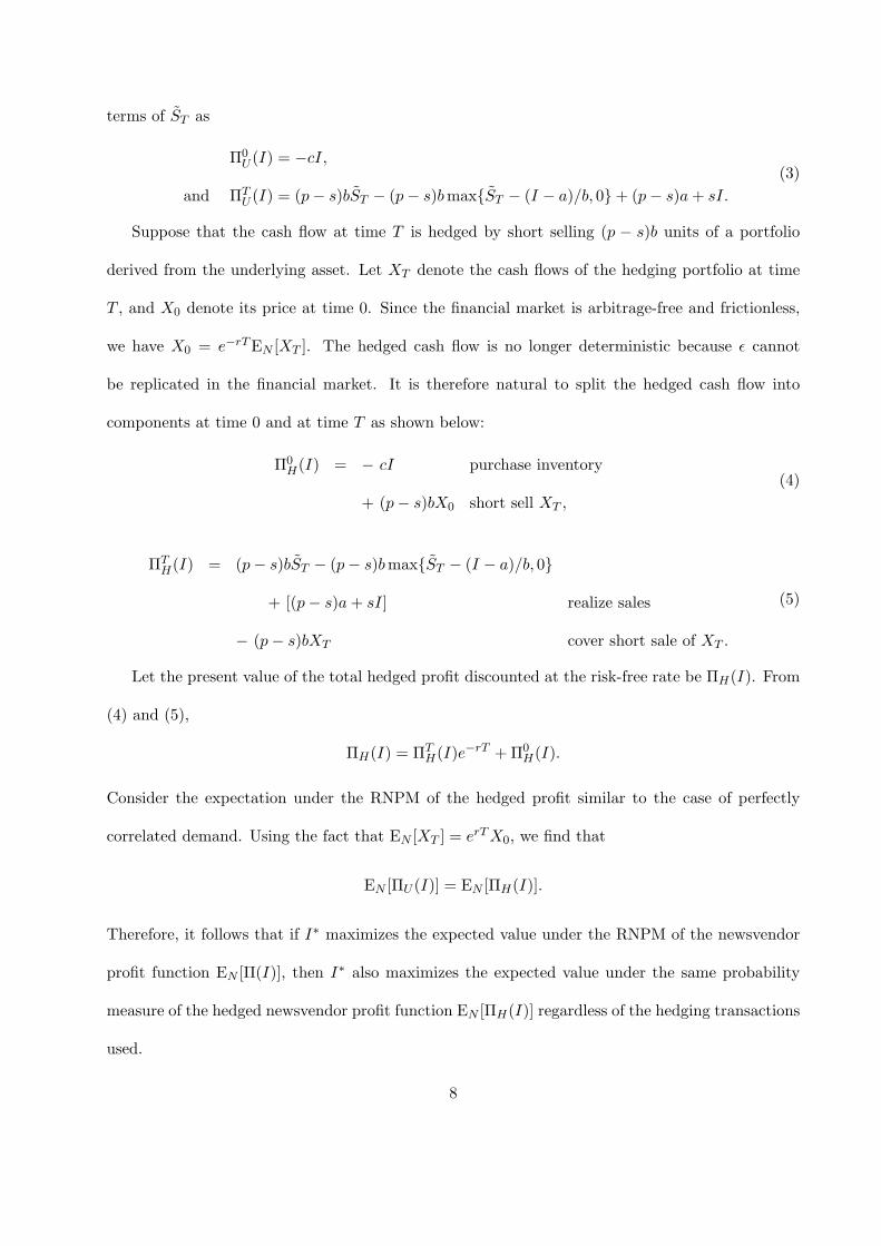
terms of ST as

Π0U (I) = −cI,

and ΠTU (I) = (p− s)bST − (p− s)b max{ST − (I − a)/b, 0}+ (p− s)a + sI.

(3)

Suppose that the cash flow at time T is hedged by short selling (p − s)b units of a portfolio

derived from the underlying asset. Let XT denote the cash flows of the hedging portfolio at time

T , and X0 denote its price at time 0. Since the financial market is arbitrage-free and frictionless,

we have X0 = e−rT EN [XT ]. The hedged cash flow is no longer deterministic because ε cannot

be replicated in the financial market. It is therefore natural to split the hedged cash flow into

components at time 0 and at time T as shown below:

Π0H(I) = − cI purchase inventory

+ (p− s)bX0 short sell XT ,

(4)

ΠTH(I) = (p− s)bST − (p− s)b max{ST − (I − a)/b, 0}

+ [(p− s)a + sI] realize sales

− (p− s)bXT cover short sale of XT .

(5)

Let the present value of the total hedged profit discounted at the risk-free rate be ΠH(I). From

(4) and (5),

ΠH(I) = ΠTH(I)e−rT + Π0

H(I).

Consider the expectation under the RNPM of the hedged profit similar to the case of perfectly

correlated demand. Using the fact that EN [XT ] = erT X0, we find that

EN [ΠU (I)] = EN [ΠH(I)].

Therefore, it follows that if I∗ maximizes the expected value under the RNPM of the newsvendor

profit function EN [Π(I)], then I∗ also maximizes the expected value under the same probability

measure of the hedged newsvendor profit function EN [ΠH(I)] regardless of the hedging transactions

used.

8

However, it is no longer possible to hedge the inventory risk perfectly. As a consequence,

unlike the case in §2, we cannot provide a no-arbitrage argument for the use of RNPM to compute

the optimal inventory level. Moreover, different decision-makers could prefer different hedging

transactions depending on their utility functions. Therefore, from hereforward, we assume that the

decision-maker is risk-averse. We use the subjective probability measure in our analysis. In §3.1,

we analyze the hedged payoff (5) in the mean-variance framework. In §3.2, we provide results for

more general utility functions.

3.1 Minimum Variance Hedge

Minimum variance hedging is a common solution concept used for a risk-averse decision-maker

(see, for example, Hull 2002: Chapter 2). Therefore, in this section, we first determine the optimal

hedging portfolio XT that minimizes the variance of the payoff at time T for a given inventory

level I, and then consider a heuristic hedge comprised of fewer financial transactions. Finally,

in §3.1.1, we examine dynamic hedging, i.e., the re-balancing of the hedging portfolio when new

information regarding the asset price and the demand forecast becomes available over time. The

optimal solution to the problem of minimizing the variance of ΠTH(I) with respect to XT for given

I can be obtained from a standard result in probability theory, see for example, §9.4 in Williams

(1991). Specifically,

Lemma 1. The variance of ΠTH(I) is minimized by setting X∗

T = Eε

[ΠT

U (I)∣∣ ST

].

Proof: Omitted. 2

Fig. 3 depicts the cash flows of the minimum variance hedge as a function of ST . For comparison,

it also shows the hedging portfolio when ε = 0. It can easily be shown that the hedge is a concave

increasing function of ST . Thus, the hedge can be approximated by short selling the underlying

asset and purchasing a series of call options with settlement date T and different exercise prices.

9

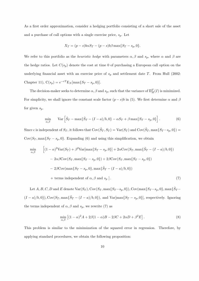
As a first order approximation, consider a hedging portfolio consisting of a short sale of the asset

and a purchase of call options with a single exercise price, sp. Let

XT = (p− s)bαST − (p− s)bβ max{ST − sp, 0}.

We refer to this portfolio as the heuristic hedge with parameters α, β and sp, where α and β are

the hedge ratios. Let C(sp) denote the cost at time 0 of purchasing a European call option on the

underlying financial asset with an exercise price of sp and settlement date T . From Hull (2002:

Chapter 11), C(sp) = e−rT EN [max{ST − sp, 0}].

The decision-maker seeks to determine α, β and sp, such that the variance of ΠTH(I) is minimized.

For simplicity, we shall ignore the constant scale factor (p− s)b in (5). We first determine α and β

for given sp.

minα,β

Var[ST −max{ST − (I − a)/b, 0} − αST + β max{ST − sp, 0}

]. (6)

Since ε is independent of ST , it follows that Cov(ST , ST ) = Var(ST ) and Cov(ST ,max{ST−sp, 0}) =

Cov(ST ,max{ST − sp, 0}. Expanding (6) and using this simplification, we obtain

minα,β

[(1− α)2Var(ST ) + β2Var[max{ST − sp, 0}] + 2αCov(ST ,max{ST − (I − a)/b, 0})

− 2αβCov(ST ,max{ST − sp, 0}) + 2βCov(ST ,max{ST − sp, 0})

− 2βCov(max{ST − sp, 0},max{ST − (I − a)/b, 0})

+ terms independent of α, β and sp ] . (7)

Let A,B, C, D and E denote Var(ST ),Cov(ST ,max{ST−sp, 0}),Cov(max{ST−sp, 0},max{ST−

(I − a)/b, 0}),Cov(ST ,max{ST − (I − a)/b, 0}), and Var[max{ST − sp, 0}], respectively. Ignoring

the terms independent of α, β and sp, we rewrite (7) as

minα,β

[(1− α)2A + 2β(1− α)B − 2βC + 2αD + β2E

]. (8)

This problem is similar to the minimization of the squared error in regression. Therefore, by

applying standard procedures, we obtain the following proposition:

10

Proposition 1. If sp > 0, then the function in (8) is strictly convex in α and β, and the minimum

variance hedge is obtained by setting

α = 1− DE −BC

AE −B2(9)

β =AC −BD

AE −B2. (10)

Proof: Omitted.

Now consider the choice of sp. As pointed out by a referee, it is no longer optimal in general

to set sp = (I − a)/b as was in the case of perfectly correlated demand in §2. Further, we found

examples in which the variance function is not jointly quasi-convex in α, β and sp. Therefore, the

optimal value of sp has to be determined numerically by doing a line search on sp with the values

of α and β as given by Proposition 1. This method gives the correct answer since the variance is

strictly convex in α and β for a given sp.

The following example illustrates how the variance of the hedged profit behaves as a function

of sp.

Example. Let S0 = $660, r = 10% per annum, and ST have a log-normal distribution with

µ = 10% per annum and σ = 20% per annum. Let T = 6 months. Let the demand for the

item be 10ST + ε, where ε is normally distributed with mean 0 and standard deviation 600. Let

p = $1, c = $0.60 and s = $0.10.

Let I = 7000. The variance of the unhedged profit function is equal to 371,280. Fig. 4 shows

the variance of the hedged profit as a function of sp for different values of α and β. While (I−a)/b

is equal to 700, the optimal value of sp differs from 700 for each set of α and β values. For example,

when α = 1.1 and β = 0.8, then the minimum variance is 161,301 and is realized at sp = 630; when

α = 0.65 and β = 0.9, then the minimum variance is 155,145 and is realized at sp = 770. The

global optimal solution is α = β = 0.75 and sp = 722, and gives a variance of 146,400.

11

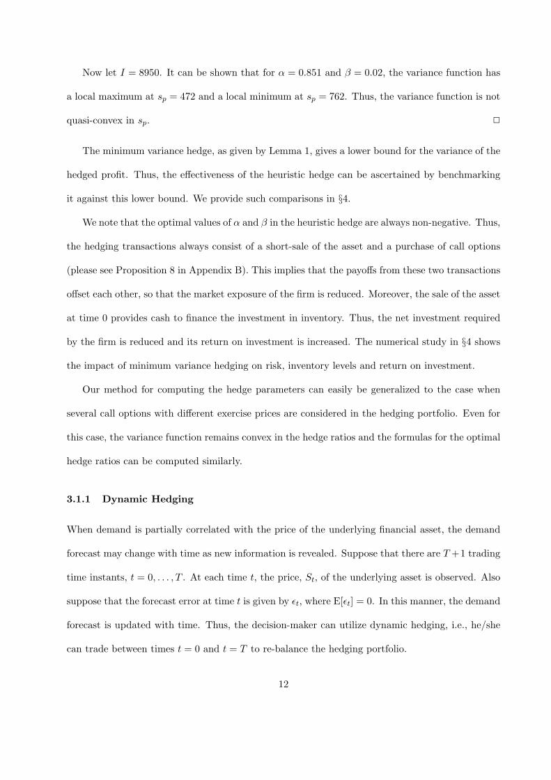
Now let I = 8950. It can be shown that for α = 0.851 and β = 0.02, the variance function has

a local maximum at sp = 472 and a local minimum at sp = 762. Thus, the variance function is not

quasi-convex in sp. 2

The minimum variance hedge, as given by Lemma 1, gives a lower bound for the variance of the

hedged profit. Thus, the effectiveness of the heuristic hedge can be ascertained by benchmarking

it against this lower bound. We provide such comparisons in §4.

We note that the optimal values of α and β in the heuristic hedge are always non-negative. Thus,

the hedging transactions always consist of a short-sale of the asset and a purchase of call options

(please see Proposition 8 in Appendix B). This implies that the payoffs from these two transactions

offset each other, so that the market exposure of the firm is reduced. Moreover, the sale of the asset

at time 0 provides cash to finance the investment in inventory. Thus, the net investment required

by the firm is reduced and its return on investment is increased. The numerical study in §4 shows

the impact of minimum variance hedging on risk, inventory levels and return on investment.

Our method for computing the hedge parameters can easily be generalized to the case when

several call options with different exercise prices are considered in the hedging portfolio. Even for

this case, the variance function remains convex in the hedge ratios and the formulas for the optimal

hedge ratios can be computed similarly.

3.1.1 Dynamic Hedging

When demand is partially correlated with the price of the underlying financial asset, the demand

forecast may change with time as new information is revealed. Suppose that there are T +1 trading

time instants, t = 0, . . . , T . At each time t, the price, St, of the underlying asset is observed. Also

suppose that the forecast error at time t is given by εt, where E[εt] = 0. In this manner, the demand

forecast is updated with time. Thus, the decision-maker can utilize dynamic hedging, i.e., he/she

can trade between times t = 0 and t = T to re-balance the hedging portfolio.

12

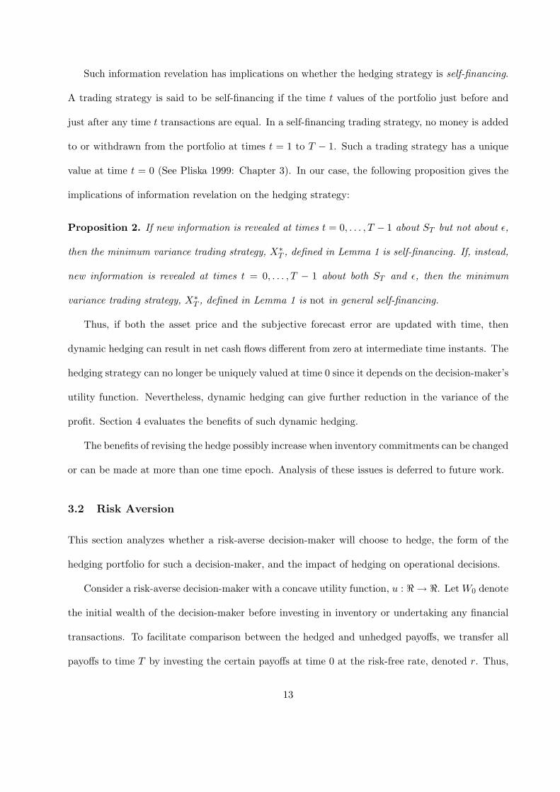
Such information revelation has implications on whether the hedging strategy is self-financing.

A trading strategy is said to be self-financing if the time t values of the portfolio just before and

just after any time t transactions are equal. In a self-financing trading strategy, no money is added

to or withdrawn from the portfolio at times t = 1 to T − 1. Such a trading strategy has a unique

value at time t = 0 (See Pliska 1999: Chapter 3). In our case, the following proposition gives the

implications of information revelation on the hedging strategy:

Proposition 2. If new information is revealed at times t = 0, . . . , T − 1 about ST but not about ε,

then the minimum variance trading strategy, X∗T , defined in Lemma 1 is self-financing. If, instead,

new information is revealed at times t = 0, . . . , T − 1 about both ST and ε, then the minimum

variance trading strategy, X∗T , defined in Lemma 1 is not in general self-financing.

Thus, if both the asset price and the subjective forecast error are updated with time, then

dynamic hedging can result in net cash flows different from zero at intermediate time instants. The

hedging strategy can no longer be uniquely valued at time 0 since it depends on the decision-maker’s

utility function. Nevertheless, dynamic hedging can give further reduction in the variance of the

profit. Section 4 evaluates the benefits of such dynamic hedging.

The benefits of revising the hedge possibly increase when inventory commitments can be changed

or can be made at more than one time epoch. Analysis of these issues is deferred to future work.

3.2 Risk Aversion

This section analyzes whether a risk-averse decision-maker will choose to hedge, the form of the

hedging portfolio for such a decision-maker, and the impact of hedging on operational decisions.

Consider a risk-averse decision-maker with a concave utility function, u : < → <. Let W0 denote

the initial wealth of the decision-maker before investing in inventory or undertaking any financial

transactions. To facilitate comparison between the hedged and unhedged payoffs, we transfer all

payoffs to time T by investing the certain payoffs at time 0 at the risk-free rate, denoted r. Thus,

13

the expected utility of the decision-maker after purchasing inventory I takes the form

E [u (ΠU (I))] = E[u

(W0e

rT + (p− s)b min{ST + ε, (I − a)/b}+ (p− s)a− (cerT − s)I)]

.

Without loss of generality, we scale all cash flows by 1/(p−s)b. Let c1 denote (cerT −s)/{(p−s)b},

and W denote {W0erT +(p−s)a}/{(p−s)b}. Thus, we write ΠU (I) = min{ST + ε, (I−a)/b}− c1I

and

E [u (ΠU (I))] = E [u (W + min{ST + ε, (I − a)/b} − c1I)] . (11)

The decision-maker can access the financial market and construct a portfolio derived from the

underlying asset ST at zero transaction cost. Given this alternative, the decision-maker may or

may not prefer to invest in inventory depending on the parameters of the newsvendor model. The

following proposition specifies the range of parameter values under which the decision-maker prefers

to invest in inventory.

Proposition 3. Any risk-averse decision-maker with utility function, u(·), prefers to invest in

inventory I than to invest solely in the financial market if c1I < EN [Eε[min{ST + ε, (I−a)/b}|ST ]].

In particular, the decision-maker prefers to invest in inventory I if c1I < EN [min{ST , (I−a)/b}]−

E[|ε|] and does not prefer to invest in inventory I if c1I > EN [min{ST , (I − a)/b}].

This result can be explained as follows: the payoff Eε[min{ST + ε, (I − a)/b}|ST ] can be con-

structed from derivative instruments with ST as the underlying asset. This payoff is larger than

ΠU +c1I in the second order stochastic dominance sense and costs EN [Eε[min{ST +ε, (I−a)/b|ST }]].

Thus, if c1I > EN [Eε[min{ST + ε, (I − a)/b|ST }]], then we obtain a financial asset that is preferred

to the profits from inventory I and costs less than the investment of c1I in inventory. Thus, any

risk-averse decision-maker chooses to invest in this asset rather than in inventory level I.

In the rest of the analysis, we assume that c1I is such that the decision-maker prefers to invest

in inventory I. Let there be a hedging portfolio with the random payoff at time T denoted as XT ,

and the price at time 0 denoted as X0. We assume that XT is a fair gamble, i.e., e−rT XT is a

14

martingale and the decision maker must construct the hedge subject to this assumption. Thus, we

require that

E[XT −X0erT ] = 0. (12)

If, instead, XT had a positive risk premium then there will be two effects of investing in XT on the

decision-maker’s expected utility, a wealth effect and a risk-reduction effect. By assuming that XT

is a fair gamble, we examine the risk-reduction aspect while controlling for the wealth effect.

First consider the problem of determining XT such that the expected utility of the decision-

maker is maximized for a given inventory level I, i.e.,

max E[u

(W + ΠU (I)−XT + X0e

rT)]

such that E[XT −X0erT ] = 0. (13)

The following proposition specifies the form of the hedge using the Karush-Kuhn-Tucker conditions

(KKT). It provides broad insights but is primarily useful for the purposes of constructing an optimal

hedge:

Proposition 4. For a strictly concave utility function, u(·), the optimal solution of problem (13)

is given by X∗∗T that satisfies the following equations for some λ ∈ <:

Eε

[u′

(W + ΠU (I)−X∗∗

T + X∗∗0 erT

)]= λ,

E[X∗∗T −X∗∗

0 erT ] = 0.

For example, note that for a quadratic utility function, Proposition 4 yields the same solution as

given in Lemma 1. To see this, let u(x) = ax− bx2/2 where a, b > 0. Then, Proposition 4 gives

Eε

[a− b

(W + ΠU (I)−X∗∗

T + X∗∗0 erT

)]= a− b

(W −X∗∗

T + X∗∗0 erT

)− bEε [ΠU (I)] = λ.

Since a, b, W are constants, X∗∗T = Eε [ΠU (I)] = X∗

T is an optimal solution to the above problem.

As stated in §3.1, Fig. 3 depicts X∗T as a function of ST . Optimal hedges for other utility functions

could be similarly derived.

15

We now consider the questions whether the expected utility of the decision-maker increases with

hedging, and whether the optimal inventory level increases in the degree of hedging. In practice,

simpler hedges than that in Proposition 4 may be used. Therefore, we consider a fairly general class

of hedges in the remaining analysis. We assume that XT is an increasing function of ST because it

should offset the subject cash flows as closely as possible. The minimum variance hedge considered

in §3.1 satisfies this assumption. The heuristic hedge in §3.1 also satisfies this assumption when

β ≤ α regardless of the value of sp. Further, the hedging strategy permits the use of several call

options with different exercise prices in order to match ΠU more closely. To facilitate the analysis,

we also assume that XT is a piecewise continuous function of ST , and is differentiable with respect

to ST almost everywhere.

The following properties of utility functions are useful in the remaining analysis. The Arrow and

Pratt measure of absolute risk aversion of a utility function u(·) of wealth w is defined as the ratio

RA(w) = −u′′(w)/u′(w) (Arrow 1971). Note that RA(w) is always non-negative for an increasing

concave utility function. The utility function is said to display decreasing absolute risk aversion

(DARA) when RA(w) is decreasing in w, and constant absolute risk aversion (CARA) when RA(w)

is a constant. Both DARA and CARA further imply that u′′(w) is decreasing in absolute value (i.e.,

u′′′(w) ≥ 0). Absolute prudence is defined as the ratio −u′′′(w)/u′′(w) (Kimball 1990). Decreasing

or constant absolute prudence imply that u′′′(w) is decreasing in w. Many commonly used classes

of utility functions, such as the power utility function, the negative exponential utility function and

the logarithmic utility function, satisfy the properties of constant or decreasing absolute prudence

(DAP).

Suppose that the risk-averse firm shorts an amount α of the portfolio XT . Thus, the expected

utility of the decision-maker from the investment in inventory and the hedging transactions is given

by

E [u (ΠH(I, α))] = E[u

(W + min{ST + ε, (I − a)/b} − c1I − αXT + αX0e

rT)]

. (14)

16

Proposition 5 shows that a risk-averse decision-maker prefers the hedged newsvendor payoff to the

unhedged newsvendor payoff for any given I.

Proposition 5. For any concave and differentiable utility function, u(·),

d

dαE [u (ΠH(I, α))]

∣∣∣∣α=0

≥ 0. (15)

While this result by itself is not surprising, it should be considered as a counterpart to Propo-

sition 3. Together they show that under appropriate conditions, a risk-averse decision-maker will

both invest in inventory as well as hedge the risk using financial instruments. We now examine

the implications of hedging on the optimal inventory level. Propositions 6 and 7 give two sufficient

conditions under which the optimal stocking quantity chosen by a risk-averse decision-maker in-

creases when he/she decides to hedge the newsvendor risk. Given the utility function, Proposition

6 gives a sufficient condition on the structure of the hedging portfolio, derived using the form of

the newsvendor payoff and Jensen’s inequality. Given the hedging portfolio, Proposition 7 gives a

sufficient condition on the utility function.

Proposition 6. For any increasing, concave and differentiable utility function, u(·), the value of

inventory that maximizes E[u(ΠH)] is greater than the value of inventory that maximizes E[u(ΠU )]

if XT is such that

E[{u′(ΠH(I))− u′(ΠU (I))} · 1{ε ≤ (I − a)/b− ST }] ≤ 0, (16)

and E[u′((I − a)/b− c1I − αXT + αX0e

rT )]− u′((I − a)/b− c1I) ≥ 0. (17)

If u(·) is additionally CARA or DARA, then (17) is automatically satisfied.

Proposition 6 is primarily useful for constructing an optimal hedge. The intuitive content of

the proposition is that when ST , and thus, ΠU is small (i.e., when (16) applies), then the hedge

increases the utility of the decision-maker. On the other hand, when ST is large (i.e., when (17)

applies), then the hedge decreases the utility of the decision-maker.

17

Proposition 7 considers hedging portfolios that are increasing in ST and gives a sufficient condi-

tion on the decision-maker’s utility function. Thus, it supplements the result in Proposition 6. Let

I∗(α) ≡ arg maxI{E[u(ΠH(I, α))]} denote the stocking quantity that maximizes expected utility for

a given value of α. Also let α be the largest value of α such that Eε[ΠH(I, α)|ST ] is non-decreasing

in ST . We focus attention on hedging ratios in the range 0 ≤ α ≤ α because higher values of α

correspond to overhedging.

Proposition 7. For any increasing, concave and differentiable utility function, u(·), with constant

or decreasing absolute risk aversion and constant or decreasing absolute prudence, dI∗/dα ≥ 0 for

0 ≤ α ≤ α.

We relate these results to the research on the impact of risk-aversion on operational decisions,

and specifically, on the newsvendor model. Eeckhoudt, et al. (1995) show that the optimal inventory

level for a risk-averse newsvendor is lower than that for a risk-neutral newsvendor under both CARA

and DARA preferences. Similar conclusions are to be found in Agrawal and Seshadri (2000) and

Chen and Federgruen (2000). Propositions 6 and 7 adds to the above research by showing that

financial hedging changes the optimal inventory decision for a risk-averse newsboy under various

conditions. In particular, financial hedging increases the optimal inventory level for the risk-averse

newsvendor, and brings it closer to the risk-neutral profit-maximizing quantity. Thus, it increases

expected profit, decreases the effect of risk-aversion and brings the market closer to efficiency.

We also note that Eeckhoudt, et al. (1995) make similar assumptions on the utility function

as in Proposition 7, and show that the optimal inventory level decreases when an uncorrelated

background risk is added. Our result differs from them since the new risk XT is correlated with

the investment in inventory. Therefore, while Eeckhoudt, et al. (1995) find that optimal inventory

decreases with the addition of the background risk, we find that the optimal inventory increases

with hedging.

18

4 Numerical Example

In this section, we quantify the impact of our method on expected profit, risk reduction and return

on investment using a numerical example. We show how the benefits of hedging change with the

degree of correlation of demand with the price of the underlying financial asset, with the volatility

of the asset price, and with dynamic hedging. The example is based on sales data for computer

games CDs sold at a consumer electronics retailing chain.

We are given the following datasets:

1. A fit sample consisting of historical monthly forecasts and sales data for 42 items for one year

aggregated across all stores in the chain. The total number of observations is 216 because the

items have short lifecycles and not all items are sold in each month.

2. A test sample consisting of demand forecasts for 10 items for one month in the subsequent

year.

Let t = 1, . . . , t0 denote time indices in the fit sample, and T denote the time index in the test

sample, T > t0. Let xit and yit, respectively, denote the forecast and the unit sales for item i

in month t aggregated across all stores, and St denote the value of the S&P 500 index at the

end of month t. We first fit a forecasting equation to the fit sample. Then, using the estimated

parameters, we compute the optimal inventory level, the hedging parameters, the expected profit

and the standard deviation of profit for the test sample.

To estimate the effect of correlation of demand with St on the performance variables, we perturb

the fit sample by adding independent and identically distributed (i.i.d.) errors ξit to yit. Let

yit = yit + ξit. Here, ξit has normal distribution with mean 0. Results are computed for various

values of the standard deviation of ξit to ascertain the effect of decreasing correlation of demand with

St. In this paper, we report results for two datasets, the original dataset and the perturbed dataset

with the standard deviation of ξit equal to 15. These datasets are labeled A and B, respectively.

19

To estimate the effect of the volatility of ST on the performance variables, we consider six

scenarios for each dataset assuming that the inventory decision is taken 1, 2, . . . , 6 months in advance

of time T . Let l denote the lead-time and T − l denote the time when the order is placed. The

longer the lead-time, the greater is the volatility of ST .

For both the datasets in the fit sample, we estimate the following forecasting equations using

linear regression.

yit = m1 + m2xit + bSt + εit (18)

yit = m′1 + m′

2xit + ε′it. (19)

Here, the error terms, εit and ε′it, are assumed to be i.i.d. normally distributed.5 The coefficients

m1,m2,m′1,m

′2 and b are assumed to be identical across items and over time.6 Note that the

comparison between the forecasting equations, (18) and (19), remains fair when ξit are added to

yit. Table 2 shows the estimation results for (18) and (19). The coefficient of St is statistically

significant (p < 0.001 in each case), showing that (18) is more appropriate than (19) for modeling

demand. However, note that while (18) has a higher R2, it does not imply a lower forecast error

because St is a random variable. Thus, the benefit of using (18) is that it provides a method to

incorporate market information in forecasting demand, not that it reduces forecast error.

We compute the volatility of the S&P 500 index using 90 days of historical data prior to the

time of inventory decision for month T by the method given in Hull (2002: Section 11.3). The

volatility is given by the standard deviation of log(Sd/Sd−1), where Sd is the closing value of the

index for day d. The value of the daily standard deviation is obtained as 1.3984%, and the annual5The sales of a given item at a given store may not be normally distributed since they are truncated by the

inventory level. However, normal distribution is a fair approximation for the sum of sales across a large number of

stores.6The coefficient b is identical across items since we do not expect items in the product category to have different

degrees of correlation with economic factors. Likewise, the coefficients m1, m2, m′1, m

′2 are identical across items since

we do not expect dissimilar biases in the forecasts of different items.

20

standard deviation as 22.1982% assuming 252 trading days in the year. The risk-free rate of return

is assumed to be 5% per year.

Optimal Inventory Level and Expected Profit: Using the estimates of model (18), the

demand forecast for item i in the test sample can be written as

DiT = a + bST + εiT , (20)

where a = m1 + m2xiT . We compute the optimal inventory level and the profit with and without

hedging in this model. As a benchmark, we compute the inventory level and profit for model (19).

Note that in (19), the demand forecast for item i in the test sample is given by m′1 + m′

2xiT + ε′iT .

Table 3 compares the inventory levels and the expected profits obtained using demand dis-

tributions estimated from the two forecasting models. Results are reported for one item in the

test sample. Other items give similar insights. We find that using (18) instead of (19) changes

the inventory decision significantly and increases the expected profit by 5.1 to 6.6% for differ-

ent datasets. The values of the standard deviation show that the increase in expected profit is

statistically significant. The reasons for the increase are as follows:

1. The two models use different probability distributions for the forecast error. In (19), the

forecast error ε′it is normally distributed, whereas in (18), the distribution of the forecast

error is a convolution of the lognormal distribution of St and the normal distribution of εit.

Since the lognormal distribution is skewed to the right, the convolution results in a higher

inventory level. See Fig. 5 for a Q-Q plot of the demand distribution.

2. In model (18), up-to-date information from the financial markets has been used to augment

the firm’s historical data. Thus, forecasts based on (18) adjust to changes in St. When the

market moves up, the forecasts are revised upwards, and vice versa.

By comparing the results for different values of l, we find that model (18) enables the decision

21

maker to respond to the increase in volatility of St by increasing the inventory level while model

(19) does not. Further, hedging gives a greater reduction of risk as the volatility of St increases, as

shown below.

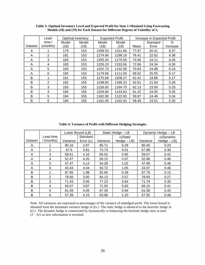
Risk and Investment: Table 4 compares the variance of unhedged profit at the optimal inven-

tory level with the variance of hedged profit. It compares results from the minimum variance hedge

of §3.1 and from the heuristic hedge of §3.1 with no re-balancing of the hedging portfolio (static

hedge), and with a re-balancing of the hedging portfolio once at time T − l/2 (dynamic hedge).

Since the minimum variance hedge gives a lower bound on the variance of hedged profit, it provides

a benchmark for the static and the dynamic hedges.

The static hedge parameters, α, β, and sp, are computed as described in §3.1. The dynamic

hedge is computed by dynamic programming. Thus, at time T − l/2, the following actions take

place: (i) the asset price ST−l/2 and the preliminary forecast error, εT−l/2 are observed;7 (ii) the

hedge parameters, α1, β1, and sp1), are computed. These hedge parameters yield the cash flows at

time T − l/2. Thus, the hedge parameters at time 0, α0, β0, and sp0, are then computed in order

to hedge the cash flows at time T − l/2.

From Proposition 2, re-balancing the hedge is not a self-financing activity since it uses informa-

tion about εT−l/2. Thus, we re-invest the cash flow at time T − l/2 at the risk-free rate in order to

evaluate the variance of hedged profit at time T . Identical series of sample paths are used to eval-

uate all hedging strategies. Many simulation runs are conducted to compute average performance

statistics and estimate the statistical significance of the results.

All figures in Table 4 are expressed as percentages of the variance of unhedged profit. We find

that the lower bound on the variance of hedged profit varies between 87.7% and 43.4%. Thus,

the potential reduction in variance that can be obtained by hedging varies between 12.4% - 56.6%.7We assume that the subjective forecast is re-evaluated at time T − l/2, and that the forecast error is a sum of two

components, εT−l/2 observed at time T−l/2, and εT observed at time T . Here, we let Var[εT−l/2] = Var[εT ] = Var[ε]/2.

22

Static hedging has a gap of about 6% with respect to the lower bound. This gap is statistically

significant at p=0.01. Dynamic hedging realizes almost the full potential for variance reduction.

Its gap with respect to the lower bound is about 0.4%, and is not statistically significant. This

performance is notable since both dynamic and static hedging use only two financial instruments.

Particularly, the results on dynamic hedging show that even though the decision-maker is unable

to modify the inventory level after time t, it can still use new information to manage its exposure

to risk.

We further find that the percent reduction in variance increases significantly with the volatility

of St. For example, for dataset A, the percent reduction in variance under the minimum variance

hedge is 20% when l = 1 and 56.6% when l = 6. Thus, hedging is more beneficial when the market

volatility is high, or equivalently, when the lead-time is longer. As expected, we also find that the

percent reduction in variance decreases when demand is less correlated with St.

Table 5 shows the initial investment in inventory with and without hedging for each scenario

corresponding to Table 5. Note that hedging reduces the initial investment by about 60% because

the inflow from the short sale of the stock offsets the cash required for buying inventory and call

options. Further, the investment decreases as the volatility of St increases. This is surprising

because we would expect both the amount of inventory and the price of the call option to increase

with volatility, resulting in larger investment. However, we find that α increases with volatility.

Thus, a larger quantity of the underlying asset is sold short, offsetting the additional investment

required in inventory and call options.

Therefore, from Tables 4 and 5, we conclude that the benefits of hedging increase with the

volatility of St. Interestingly, this implies that items with longer lead times will benefit more from

hedging than those with shorter lead times.

23

Risk-averse Decision-maker: To evaluate the effect of hedging on the optimal inventory de-

cision of the risk-averse decision-maker, we assume the expected utility representation E[u(w)] =

E[w] − ρVar[w], where w denotes wealth. The value of ρ is taken as 0.01. Table 6 presents the

inventory levels that maximize the expected utility for each of the 10 items in the test sample with

and without hedging. Observe that hedging increases the optimal inventory level. It brings the

inventory level closer to the expected value maximizing quantity, restoring efficiency in the market.

5 Conclusions

We have shown how to generate a solution to the hedging of inventory risk using the newsvendor

model when demand is correlated with the price of a financial asset. Hedging reduces the variance

of profit and the investment in inventory, increases the expected utility of a risk-averse decision-

maker, and increases the optimal inventory level for a broad class of utility functions. Our numerical

analysis shows that hedging is more beneficial when the price of the underlying asset is more volatile

or the product has a longer order lead-time. Dynamic hedging provides additional risk reduction

even when the retailer cannot change her initial inventory commitment.

Our forecasting model could be extended to incorporate macroeconomic variables such as inter-

est rates and foreign exchange rates that provide demand signals. It might also be customized for

specific businesses by using more securities from the equities market, such as sector specific indices

or portfolios of firms in similar businesses. Further, the evolution of the price of the underlying

asset may be used to update the demand forecast and modify order quantities even in the absence

of early demand data.

An important aspect of our analysis is that the demand risk is not fully spanned by the financial

market. Our analysis of the effects of financial hedging on operational decisions under such a

scenario may be extended to other problems that have been considered in the real options literature,

such as production switching (Dasu and Li (1997), Huchzermeier and Cohen (1996), Kouvelis

24

(1999)), capacity planning (Birge 2000) and global contracting (Scheller-Wolfe and Tayur 1999).

References

Agrawal, V., S. Seshadri. 2000a. Effect of Risk Aversion on Pricing and Order Quantity Decisions.

Manufacturing and Service Operations Management Journal 2(4) 410-423.

Agrawal, V., S. Seshadri. 2000b. Risk intermediation in supply chains. IIE TRANSACTIONS 32(9)

819-831.

Arrow, K. 1971. Essays in the Theory of Risk-Bearing. North-Holland, Amsterdam.

Birge, J. 2000. Option Methods for Incorporating Risk into Linear Capacity Planning Models.

Manufacturing & Services Operations Management 2(1) 19-31.

Brennan, M., E. Schwartz. 1985. Evaluating Natural Resource Investments. Journal of Busi-

ness 58(2) 135-157.

Chen, F., A. Federgruen. 2000. Mean-Variance Analysis of Basic Inventory Models. Working

Paper, Graduate School of Business, Columbia University.

Copeland, T., V. Antikarov. 2001. Real Options: A Practitioner’s Guide. Texere Publishers,

London.

Dasu, S., L. Li. 1997. Optimal Operating Policies in the Presence of Exchange Rate Variability.

Management Science 43(5) 705-722.

Eeckhoudt, L., C. Gollier, H. Schlesinger. 1995. The Risk-averse (and Prudent) Newsboy. Man-

agement Science 41(5) 786-794.

Hadley, G., T. M. Whitin. 1963. Analysis of Inventory Systems. Prentice-Hall Inc., Englewood

Cliffs, New Jersey.

25

Huang, C. F., R. H. Litzenberger. 1988. Foundations for Financial Economics. Prentice-Hall

Inc., Englewood Cliffs, New Jersey.

Huchzermeier, A., M. Cohen. 1996. Valuing Operational Flexibility Under Exchange Rate Risk.

Operations Research 44(1) 100-113.

Hull, J. C. 2002. Options, Futures, and Other Derivatives. 4th ed., Prentice-Hall Inc., Englewood

Cliffs, New Jersey.

Instinet Research. 2001a. Redbook Retail Sales Monthly November 2001, New York.

Instinet Research. 2001b. The Redbook Average December 4, 2001, New York.

Kimball, M. S. 1990. Precautionary Saving in the Small and in the Large. Econometrica 58(1)

53-73.

Kimball, M. S. 1993. Standard Risk Aversion. Econometrica 61(3) 589-611.

Kogut, B., N. Kulatilaka. 1994. Operating Flexibility, Global Manufacturing, and the Option

Value of Multinational Network. Management Science 40(1) 123-139.

Kouvelis, P. 1999. Global Sourcing Strategies Under Exchange Rate Uncertainty, Chapter 20

in Quantitative Models For Supply Chain Management. Eds. S. Tayur, R. Ganeshan, M.

Magazine. Kluwer Academic Publishers, Boston.

Lee, H. L., S. Nahmias. 1993. Single Product Single Location Models, Chapter 1 in Handbooks

in OR and MS, Vol. 4, Logistics of Production and Inventory. Eds. S. C. Graves, A. H. G.

Rinnooy Kan, P. H. Zipkin. North-Holland Publishers, Netherlands.

McDonald, R., D. Siegel. 1986. The Value of Waiting to Invest. The Quarterly Journal of

Economics 101(4) 707-728.

26

Pliska, S. 1999. Introduction to Mathematical Finance: Discrete Time Models. Blackwell Pub-

lishers, Malden, Massachusetts.

Porteus, E. 2002. Foundations of Stochastic Inventory Theory. Stanford University Press, Stan-

ford, CA.

Scheller-Wolfe, A., S. Tayur. 1999. Managing Supply Chains in Emerging Markets, Chapter 22

in Quantitative Models For Supply Chain Management. Eds. S. Tayur, R. Ganeshan, M.

Magazine. Kluwer Academic Publishers, Boston.

Triantis, A., J. Hodder. 1990. Valuing Flexibility as a Complex Option. Journal of Finance 45(2)

549-565.

Trigeorgis, L. 1996. Real Options. MIT Press, Cambridge, MA.

Williams, D. 1991. Probability with Martingales. Cambridge University Press, UK.

Zipkin, P. H. 2000. Foundations of Inventory Management. McGraw-Hill, New York.

27

Appendix A. Proofs

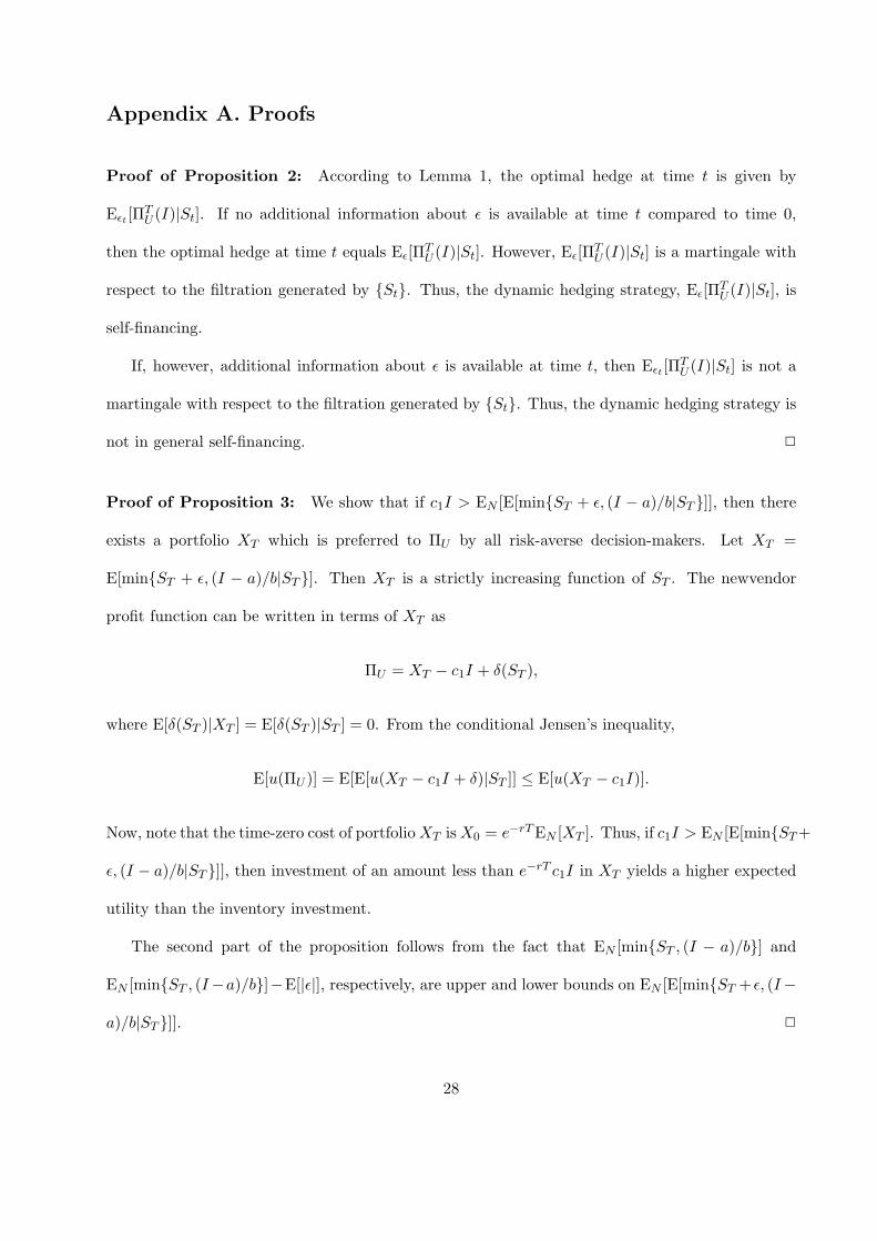
Proof of Proposition 2: According to Lemma 1, the optimal hedge at time t is given by

Eεt [ΠTU (I)|St]. If no additional information about ε is available at time t compared to time 0,

then the optimal hedge at time t equals Eε[ΠTU (I)|St]. However, Eε[ΠT

U (I)|St] is a martingale with

respect to the filtration generated by {St}. Thus, the dynamic hedging strategy, Eε[ΠTU (I)|St], is

self-financing.

If, however, additional information about ε is available at time t, then Eεt [ΠTU (I)|St] is not a

martingale with respect to the filtration generated by {St}. Thus, the dynamic hedging strategy is

not in general self-financing. 2

Proof of Proposition 3: We show that if c1I > EN [E[min{ST + ε, (I − a)/b|ST }]], then there

exists a portfolio XT which is preferred to ΠU by all risk-averse decision-makers. Let XT =

E[min{ST + ε, (I − a)/b|ST }]. Then XT is a strictly increasing function of ST . The newvendor

profit function can be written in terms of XT as

ΠU = XT − c1I + δ(ST ),

where E[δ(ST )|XT ] = E[δ(ST )|ST ] = 0. From the conditional Jensen’s inequality,

E[u(ΠU )] = E[E[u(XT − c1I + δ)|ST ]] ≤ E[u(XT − c1I)].

Now, note that the time-zero cost of portfolio XT is X0 = e−rT EN [XT ]. Thus, if c1I > EN [E[min{ST +

ε, (I − a)/b|ST }]], then investment of an amount less than e−rT c1I in XT yields a higher expected

utility than the inventory investment.

The second part of the proposition follows from the fact that EN [min{ST , (I − a)/b}] and

EN [min{ST , (I−a)/b}]−E[|ε|], respectively, are upper and lower bounds on EN [E[min{ST + ε, (I−

a)/b|ST }]]. 2

28

Proof of Proposition 4: Let λ ∈ < be the Lagrangian multiplier for the constraint E[XT −

X0erT ] = 0. The decision-maker solves the problem

max E[u

(W + ΠU (I)−XT + X0e

rT)

+ λXT − λX0erT

].

Since u is concave, the first order conditions of optimality are sufficient. The optimal solution is

obtained by maximizing the utility function point-wise at each value of ST . Thus, the first order

conditions are

Eε

[u′

(W + ΠU (I)−XT + X0e

rT)]

= λ, (21)

E[XT −X0erT ] = 0. (22)

A feasible solution to this system of equations can be found as follows. Fix λ. For each value of

ST , find XT such that (21) is satisfied. This value of XT exists and is unique because u′ is strictly

decreasing. Substitute XT into (22). If E[XT − X0erT ] > 0, then reduce λ (and correspondingly

reduce all XT ) until a solution is obtained. Otherwise, increase λ and correspondingly increase all

XT .

Suppose that there exist two distinct solutions to (21)-(22), denoted (λ, X∗∗T (λ)) and (λ′, X∗∗

T (λ′)).

Clearly, λ = λ′. This further shows that X∗∗T (λ) is equal to X∗∗

T (λ′) almost everywhere. Thus, the

two solutions are equal except possibly on a set of measure zero. 2

Proof of Proposition 5: The first derivative of the expected utility function evaluated at α = 0

gives

E[u′ (W + min{ST + ε, (I − a)/b} − c1I)

{−XT + X0e

rT}]

Here, u′(·) is a decreasing function of ST at α = 0, and −XT + X0erT is also decreasing in ST .

29

Thus, they have a positive covariance, which gives

E[u′ (W + min{ST + ε, (I − a)/b} − c1I)

{−XT + X0e

rT}]

≥ E[u′ (W + min{ST + ε, (I − a)/b} − c1I)

]E

[−XT + X0e

rT]

= 0,

where the last equality follows from (12). 2

Proof of Proposition 6: The value of inventory that maximizes E[u(ΠH)] is greater than the

value of inventory that maximizes E[u(ΠU )] if

E[{

u′(ΠH(I))− u′(ΠU (I))} ∂ΠU

∂I

]≥ 0.

Here, we have used the fact that ∂ΠH/∂I = ∂ΠU/∂I. Let G(ε) denote the distribution function of

ε. Conditioning on ST and taking expectation with respect to ε, we get

Eε

[{u′(ΠH(I))− u′(ΠU (I))

} ∂Π∂I

∣∣∣∣ ST

]= −c1

∫ (I−a)/b

−∞

{u′(ΠH(I))− u′(ΠU (I))

}dG(ε)

+{u′((I − a)/b− c1I − αXT + αX0e

rT )− u′((I − a)/b− c1I)}

Pr{ε ≥ (I − a)/b− ST }.

Consider the expectation over ST of the second term in the above equation. We use the facts that

Pr{ε ≥ (I − a)/b− ST } ≥ Pr{ε ≥ (I − a)/b}, and that ST is independent of ε to write

E[{u′((I − a)/b− c1I − αXT + αX0e

rT )− u′((I − a)/b− c1I)}Pr{ε ≥ (I − a)/b− ST }]

≥ E[{u′((I − a)/b− c1I − αXT + αX0e

rT )− u′((I − a)/b− c1I)}Pr{ε ≥ (I − a)/b}]

≥[E

[u′((I − a)/b− c1I − αXT + αX0e

rT )]− u′((I − a)/b− c1I)

]Pr{ε ≥ (I − a)/b}.

(23)

Thus, if E[u′((I − a)/b− c1I − αXT + αX0e

rT )]≥ u′((I−a)/b−c1I), then the second term is non-

negative. This inequality combined with the first term gives sufficient conditions on the hedging

30

portfolio under which the hedged optimal inventory level is larger than the unhedged optimal

inventory level.

When u(·) is CARA or DARA, then u′(·) is convex in wealth. Thus, applying Jensen’s inequality

to (23), we get

E[u′((I − a)/b− c1I − αXT + αX0e

rT )]− u′((I − a)/b− c1I)

≥ u′((I − a)/b− c1I − αE[XT −X0erT ])− u′((I − a)/b− c1I)

= 0.

2

The following lemma is a standard result. It is useful for proving Proposition 7.

Lemma 2. Let X be any random variable, and f : < → < be a decreasing function such that

E[f(X)] = 0. Then, (i) for any decreasing non-negative function w(x), E[w(X)f(X)] > 0; (ii) for

any increasing non-negative function w(x), E[w(X)f(X)] < 0.

Proof: Consider (i). Let G(X) denote the cumulative distribution function of X. Since f(x) is

decreasing in x, there exists x0 such that f(x) > 0 for all x < x0 and f(x) < 0 for all x > x0. Then,

E[w(x)f(X)] =∫ x0

0w(x)f(x)dG(x) +

∫ ∞

x0

w(x)f(x)dG(x)

>

∫ x0

0w(x0)f(x)dG(x) +

∫ ∞

x0

w(x0)f(x)dG(x)

≥ w(x0)E[f(X)]

≥ 0.

Now consider (ii). We have

E[w(x)f(X)] =∫ x0

0w(x)f(x)dG(x) +

∫ ∞

x0

w(x)f(x)dG(x)

<

∫ x0

0w(x0)f(x)dG(x) +

∫ ∞

x0

w(x0)f(x)dG(x)

≤ w(x0)E[f(X)]

≤ 0. 2

31

Proof of Proposition 7: Let the hedged profit be denoted Π (the subscript H is ignored for

simplicity.) We need to show that ∂2E[u(Π)]/∂I∂α is greater than or equal to zero. We have

∂2

∂I∂αE[u(Π)] = E

[u′′(Π)

∂Π∂I

∂Π∂α

]= E

[Eε

[u′′(Π)

∂Π∂I

∣∣∣∣ ST

]∂Π∂α

](24)

= E[−c1Eε

[u′′(Π)

∣∣ ST

] ∂Π∂α

− 1bRA(Π0)u′(Π0) Pr{ε > (I − a)/b− ST }

∂Π∂α

],(25)

where (24) follows because ∂Π/∂α is independent of ε. For (25), note that

∂Π∂I

= −c1 +1b1{ε > (I − a)/b− ST }. (26)

Also note that Π is independent of ε for ε > (I − a)/b− ST , and we write Π0 = (I − a)/b− c1I −

αXT + αX0. Finally, u′′(Π) = −RA(Π)u′(Π).

Consider Eε [u′′(Π)|ST ]. Let G(ε) denote the distribution function of ε. We have

Eε

[u′′(Π)

∣∣ ST

]=

∫ (I−a)/b−ST

−∞u′′(ST + ε− c1I − αXT + αX0)dG(ε)

+∫ ∞

(I−a)/b−ST

u′′((I − a)/b− c1I − αXT + αX0)dG(ε).

Since u′′(·) < 0, the above expression shows that Eε [u′′(Π)|ST ] is negative for all ST . Further,

differentiating Eε [u′′(Π)|ST ] with respect to ST , we get

d

dSTEε

[u′′(Π)

∣∣ ST

]=

∫ (I−a)/b−ST

−∞u′′′(ST + ε− c1I − αXT + αX0)(1− α

dXT

dST)dG(ε)

−∫ ∞

(I−a)/b−ST

u′′′((I − a)/b− c1I − αXT + αX0)αdXT

dSTdG(ε)

Let f(ε, ST ) = 1{ε < (I − a)/b − ST } − αdXT /dST . f(·) is decreasing in ε. Further, Eε[f(·)|ST ],

which is equal to the slope of Eε[Π|ST ] with respect to ST , is positive for all α ∈ [0, α]. Thus, f(·)

is a decreasing function with a non-negative conditional expectation with respect to ε.

In addition, u′′′(·) > 0 because u(·) is CARA or DARA. Further, from the assumption of

constant or decreasing absolute prudence, we have that u′′′(·) is decreasing in ε. Combining these

observations and applying Lemma 2(i), we find that Eε [u′′(Π)|ST ] is increasing in ST .

32

Consider the first term in (25): ∂Π/∂α is decreasing in ST and has zero expectation (due to

the first condition for an optimum with respect to α); −c1Eε [u′′(Π)|ST ] is decreasing in ST and

is non-negative for all ST . Thus, all conditions of Lemma 2(i) are satisfied. Therefore, applying

Lemma 2(i), we find that the first term in (25) is non-negative.

Consider the second term in (25). Here, Π0 is decreasing in ST . Thus, RA(Π0), u′(Π0), and

Pr{ε > (I − a)/b− ST } are increasing in ST ; ∂Π/∂α is decreasing in ST and has zero expectation.

Therefore, applying Lemma 2(ii), we find that the second term in (25) (i.e., 1bRA(Π0)u′(Π0) Pr{ε >

(I − a)/b− ST }∂Π∂α ) is negative.

Thus, dI∗/dα ≥ 0 for 0 ≤ α ≤ α. 2

33

Appendix B. Further Results on Minimum Variance Hedging

Proposition 8. In Proposition 1, α ≥ 0 and β ≥ 0.

Proof: To prove that β ≥ 0, it suffices to show that AC − BD ≥ 0 because AE − B2 > 0 from

Proposition 1. We first establish this inequality. We then show that β ≥ 0 implies α ≥ 0.

Let X denote min{ST , sp} and Y denote min{ST , (I − a)/b− ε}. Let ν ≡ ε + sp − (I − a)/b, so

that Y = min{ST , sp − ν}. After some algebraic manipulations, we rewrite AC −BD as

AC −BD = Var(ST )Cov(X, Y )− Cov(ST , X)Cov(ST , Y ). (27)

It turns out that this inequality is not true in general for any three random variables8. To analyze

the inequality, we simplify it further by conditioning on ν and by using the following fact: for

random variables X1 and X2 with finite first and second moments, the covariance of X1 and X2

can be expressed by conditioning on a third random variable X3 (see Feller, 1966) as

Cov(X1, X2) = E[Cov(X1|X3, X2|X3)] + Cov[E(X1|X3),E(X2|X3)]. (28)

In our case, since ε is independent of ST and X, it follows that E[ST |ν] = E[ST |ε] = E[ST ] and

E[X|ν] = E[X|ε] = E[X]. Thus, we have

Cov(X, Y ) = E[Cov(X|ν, Y |ν)] + Cov[E(X|ν),E(Y |ν)]

= E[Cov(X|ν, Y |ν)],

and

Cov(ST , Y ) = E[Cov(ST |ν, Y |ν)] + Cov[E(ST |ν),E(Y |ν)]

= E[Cov(ST |ν, Y |ν)].

Therefore, to prove that AC −BD ≥ 0, it is sufficient to show for each ν that

f(ν) ≡ Var(ST )Cov(X, Y |ν)− Cov(ST , X)Cov(ST , Y |ν) ≥ 0. (29)8For example, let Y = ST −X. The inequality (27) reduces to Cov(ST , X)2 −Var(ST )Var(X) ≤ 0.

34

The following lemmas are useful.

Lemma 3. EX ≤ EST and EX ≤ sp.

Proof: X = min{ST , sp} ≤ ST . Therefore, EX ≤ EST . The inequality is strict for sp > 0. The

second inequality follows similarly. 2

Lemma 4. Var(ST ) ≥ Cov(ST , X) ≥ Var(X) ≥ 0.

Proof: The terms for the first inequality can be rearranged to obtain Cov(ST , ST − X) ≥ 0,

or equivalently, Cov(ST ,max{ST − sp, 0}) ≥ 0. We apply an alternative method of computing

covariance (see Barlow and Proschan, 1981) to show this result.

Let X1 and X2 be any two random variables with finite first and second moments. Let X1(s) = 1

if X1 > s, 0 otherwise, and X2(s) = 1 if X2 > s, 0 otherwise. The covariance of X1 and X2 is given

by

Cov(X1, X2) =∫ ∞

−∞

∫ ∞

−∞Cov(X1(s), X2(t))ds dt. (30)

Let ST (s) = 1 if ST > s, and 0 otherwise. Similarly, let X(t) = 1 if max{ST − sp, 0} > t, 0

otherwise. The covariance of ST (s) and X(t) is given by

Cov(ST (s), X(t)) = Prob[ST > max{s, t + sp}]− Prob[ST > s]Prob[ST > t + sp].

Thus,

Cov(ST (s), X(t)) ≥ 0 for s, t ≥ 0

Cov(ST (s), X(t)) = 0 for s, t < 0.

Integrating this covariance over s and t gives the first inequality. The proofs for the second and

third inequalities are similar. 2

Lemma 5. Cov(ST , Y ) ≥ 0.

Proof: Similar to that of Lemma 4. 2

35

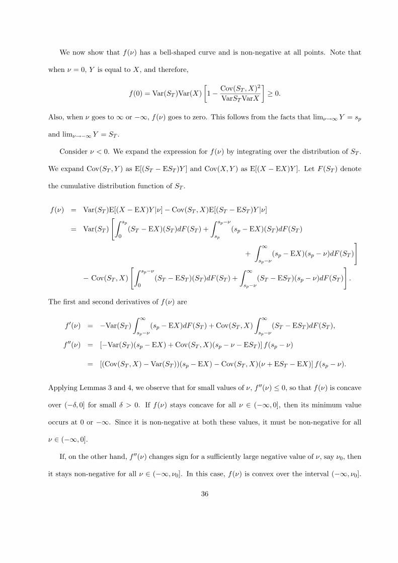
We now show that f(ν) has a bell-shaped curve and is non-negative at all points. Note that

when ν = 0, Y is equal to X, and therefore,

f(0) = Var(ST )Var(X)[1− Cov(ST , X)2

VarST VarX

]≥ 0.

Also, when ν goes to ∞ or −∞, f(ν) goes to zero. This follows from the facts that limν→∞ Y = sp

and limν→−∞ Y = ST .

Consider ν < 0. We expand the expression for f(ν) by integrating over the distribution of ST .

We expand Cov(ST , Y ) as E[(ST − EST )Y ] and Cov(X, Y ) as E[(X − EX)Y ]. Let F (ST ) denote

the cumulative distribution function of ST .

f(ν) = Var(ST )E[(X − EX)Y |ν]− Cov(ST , X)E[(ST − EST )Y |ν]

= Var(ST )

[∫ sp

0(ST − EX)(ST )dF (ST ) +

∫ sp−ν

sp

(sp − EX)(ST )dF (ST )

+∫ ∞

sp−ν(sp − EX)(sp − ν)dF (ST )

]

− Cov(ST , X)

[∫ sp−ν

0(ST − EST )(ST )dF (ST ) +

∫ ∞

sp−ν(ST − EST )(sp − ν)dF (ST )

].

The first and second derivatives of f(ν) are

f ′(ν) = −Var(ST )∫ ∞

sp−ν(sp − EX)dF (ST ) + Cov(ST , X)

∫ ∞

sp−ν(ST − EST )dF (ST ),

f ′′(ν) = [−Var(ST )(sp − EX) + Cov(ST , X)(sp − ν − EST )] f(sp − ν)

= [(Cov(ST , X)−Var(ST ))(sp − EX)− Cov(ST , X)(ν + EST − EX)] f(sp − ν).

Applying Lemmas 3 and 4, we observe that for small values of ν, f ′′(ν) ≤ 0, so that f(ν) is concave

over (−δ, 0] for small δ > 0. If f(ν) stays concave for all ν ∈ (−∞, 0], then its minimum value

occurs at 0 or −∞. Since it is non-negative at both these values, it must be non-negative for all

ν ∈ (−∞, 0].

If, on the other hand, f ′′(ν) changes sign for a sufficiently large negative value of ν, say ν0, then

it stays non-negative for all ν ∈ (−∞, ν0]. In this case, f(ν) is convex over the interval (−∞, ν0].

36

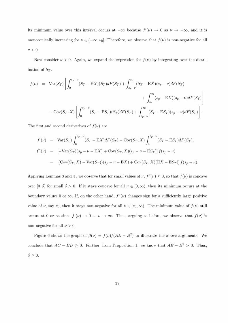
Its minimum value over this interval occurs at −∞ because f ′(ν) → 0 as ν → −∞, and it is

monotonically increasing for ν ∈ (−∞, ν0]. Therefore, we observe that f(ν) is non-negative for all

ν < 0.

Now consider ν > 0. Again, we expand the expression for f(ν) by integrating over the distri-

bution of ST .

f(ν) = Var(ST )

[∫ sp−ν

0(ST − EX)(ST )dF (ST ) +

∫ sp

sp−ν(ST − EX)(sp − ν)dF (ST )

+∫ ∞

sp

(sp − EX)(sp − ν)dF (ST )

]

− Cov(ST , X)

[∫ sp−ν

0(ST − EST )(ST )dF (ST ) +

∫ ∞

sp−ν(ST − EST )(sp − ν)dF (ST )

].

The first and second derivatives of f(ν) are

f ′(ν) = Var(ST )∫ sp−ν

0(ST − EX)dF (ST )− Cov(ST , X)

∫ sp−ν

0(ST − EST )dF (ST ),

f ′′(ν) = [−Var(ST )(sp − ν − EX) + Cov(ST , X)(sp − ν − EST )] f(sp − ν)

= [(Cov(ST , X)−Var(ST ))(sp − ν − EX) + Cov(ST , X)(EX − EST )] f(sp − ν).

Applying Lemmas 3 and 4 , we observe that for small values of ν, f ′′(ν) ≤ 0, so that f(ν) is concave

over [0, δ) for small δ > 0. If it stays concave for all ν ∈ [0,∞), then its minimum occurs at the

boundary values 0 or ∞. If, on the other hand, f ′′(ν) changes sign for a sufficiently large positive

value of ν, say ν0, then it stays non-negative for all ν ∈ [ν0,∞). The minimum value of f(ν) still

occurs at 0 or ∞ since f ′(ν) → 0 as ν → ∞. Thus, arguing as before, we observe that f(ν) is

non-negative for all ν > 0.

Figure 6 shows the graph of β(ν) = f(ν)/(AE − B2) to illustrate the above arguments. We

conclude that AC − BD ≥ 0. Further, from Proposition 1, we know that AE − B2 > 0. Thus,

β ≥ 0.

37

Now, to show that α ≥ 0, we rewrite (6) as

Var[ST −max{ST − sp, 0} − αST + β max{ST − sp, 0}

]=

Var[ST −max{ST − sp, 0}+ β max{ST − sp, 0}

]+ α2Var(ST )

− 2αCov(ST −max{ST − sp, 0}+ β max{ST − sp, 0}, ST

).

From Lemma 4, we know that Cov(ST ,max{ST − sp, 0}) = Cov(ST , ST −X) ≥ 0. From Lemma 5,

we know that Cov(ST −max{ST − sp, 0}, ST ) = Cov(Y, ST ) ≥ 0. Combining these terms and using

β ≥ 0 from above, we observe that the value of α that minimizes the variance of the hedged profit

must be non-negative. 2

38

38

Table 1: Results for the Regression of Sector-wise Redbook Same Store Sales Growth Rate on the Annual Return on the S&P 500 Index

R2 F-statistic p-value Intercept Slope

Apparel 0.411 7.6618 0.0183 -0.583 0.351 2.168 0.127

0.468 9.6673 0.0099 2.088 0.215 Department Stores 1.182 0.069

0.020 0.2298 0.6410 3.596 -0.025 Discount Stores 0.890 0.052

Note: (1) The analysis uses monthly data for 13 months from November 2000 to November 2001 for each sector. The dependent variable is the growth rate of same store sales during the month with respect to the same month in the previous year. The independent variable is the annual return on the S&P 500 index for the same period. (2) The standard errors of the parameters are reported below the corresponding parameter estimates.

Table 2: Results of the Estimation of Forecasting Models (18) and (19) for Item 1

Forecasting Model Dataset m1 m2 b R2 F-statistic

Standard Error

Equation (18) A -117.128 1.049 0.162 0.736 296.3 19.63 17.724 0.046 0.086 B -112.273 1.059 0.157 0.628 179.8 25.302 22.844 0.059 0.111

Equation (19) A 47.51 1.029 0.626 358.3 23.291 3.136 0.054 B 47.257 1.039 0.541 252.2 28.043 3.776 0.065

Notes: (1) The F-test for each regression model is statistically significant at p<0.001. (2) The standard errors of the parameters are reported below the corresponding parameter estimates.

39

Table 3: Optimal Inventory Level and Expected Profit for Item 1 Obtained Using Forecasting Models (18) and (19) for Each Dataset for Different Degrees of Volatility of St

Optimal Inventory Expected Profit Increase in Expected Profit

Dataset

Lead-time l

(months) Model (18)

Model (19)

Model (18)

Model (19) Mean

Standard Error

% Increase

A 1 179 153 1299.53 1221.66 77.87 20.41 6.37 A 2 181 153 1274.60 1198.19 76.41 22.62 6.38 A 3 183 153 1250.20 1175.55 74.65 24.11 6.35 A 4 183 153 1226.23 1153.56 72.66 24.34 6.30 A 5 183 153 1202.73 1132.09 70.63 24.98 6.24 A 6 184 153 1179.56 1111.04 68.52 25.55 6.17 B 1 181 155 1270.68 1208.27 62.41 19.88 5.17 B 2 182 155 1248.83 1186.23 62.61 21.64 5.28 B 3 183 155 1226.83 1164.70 62.13 23.00 5.33 B 4 184 155 1204.84 1143.63 61.22 24.05 5.35 B 5 184 155 1182.90 1122.93 59.97 24.49 5.34 B 6 184 155 1161.00 1102.54 58.46 24.51 5.30

Table 4: Variance of Profit with Different Hedging Strategies

Lower Bound (LB) Static Hedge – LB Dynamic Hedge – LB

Dataset Lead time l (months) Variance

Standard Error (σ) Variance

σ(Static Hedge – LB) Variance

σ(Dynamic Hedge – LB)

A 1 80.16 2.87 85.71 0.29 80.40 0.23 A 2 67.5 3.81 73.73 0.51 67.88 0.36 A 3 58.61 4.10 65.02 0.65 59.07 0.42 A 4 52.47 4.20 59.15 0.97 52.98 0.46 A 5 47.47 4.14 54.28 1.02 47.99 0.46 A 6 43.44 4.04 50.72 1.05 43.97 0.46 B 1 87.65 1.98 92.66 0.39 87.79 0.15 B 2 78.56 3.00 84.13 0.57 78.83 0.27 B 3 71.43 3.56 77.22 0.64 71.79 0.35 B 4 65.67 3.87 71.55 0.83 66.10 0.41 B 5 61.09 4.05 67.39 0.94 61.58 0.45 B 6 57.39 4.15 63.96 1.20 57.92 0.48 Note: All variances are expressed as percentages of the variance of unhedged profit. The lower bound is obtained from the minimum variance hedge in §3.1. The static hedge is identical to the heuristic hedge in §3.1. The dynamic hedge is constructed by dynamically re-balancing the heuristic hedge once at time (T – l)/2 as new information is revealed.

40

Table 5: Initial Investments Required Without Hedging and With Static Hedging for the Inventory Levels Corresponding to Tables 3 and 4

Initial Investment

Dataset Lead time l (months)

Without hedging

With static hedging

% Difference

A 1 3502.58 1573.79 55.07% A 2 3535.56 1484.95 58.00% A 3 3562.47 1449.96 59.30% A 4 3563.47 1424.20 60.03% A 5 3576.19 1417.16 60.37% A 6 3588.22 1417.31 60.50% B 1 3524.59 1761.46 50.02% B 2 3547.35 1675.63 52.76% B 3 3570.36 1634.52 54.22% B 4 3590.07 1613.15 55.07% B 5 3597.64 1596.92 55.61% B 6 3596.34 1582.51 56.00%

Table 6: Comparison of Optimal Inventory Level, Expected Profit, Standard Deviation of Profit, and

Expected Utility for Each Item for a Risk-averse Decision-maker Without and With Hedging

Optimal Inventory Level Expected Profit

Standard Deviation of Profit Expected Utility

Item Without Hedging

With Hedging

Without Hedging

With Hedging

Without Hedging

With Hedging

Without Hedging

With Hedging

1 159 165 1241.92 1288.15 82.50 89.94 1199.37 1235.72 2 159 165 1286.76 1314.75 61.97 68.18 1248.36 1268.27 3 159 165 1282.37 1311.24 61.04 68.44 1245.11 1264.39 4 160 164 1285.8 1305.33 67.40 68.67 1240.38 1258.17 5 158 164 1276.8 1306.02 64.91 74.79 1234.67 1250.09 6 158 162 1276.61 1296.39 70.19 74.87 1227.34 1240.33 7 163 171 1315.53 1340.02 60.47 53.98 1278.97 1310.88 8 163 175 1322.04 1349.92 52.85 33.29 1294.11 1338.84 9 165 175 1328.63 1350.78 55.74 19.85 1297.56 1346.84 10 164 176 1326.99 1351.23 53.48 15.85 1298.4 1348.72

Note: These results are obtained using the original dataset, i.e., ξit = 0.

41

Figure 1: Redbook Same Store Sales Growth Rate Versus Annual Return on the S&P 500 Index

y = 0.0659x + 3.1066R2 = 0.8111

0

1

2

3

4

5

6

-30 -25 -20 -15 -10 -5 0 5 10 15 20

Annual % Return on S&P 500 Index (3-month MA)

Red

book

Sam

e St

ore

Sale

s Yo

Y %

(3-m

onth

M

A)

Note: The Redbook Year-on-Year Same Store Sales Growth Rate is computed as the growth rate of same store sales during a month with respect to the same month in the previous year. We use time-series data for 25 months from November 1999 to November 2001. We compute 3-month moving averages to reduce autocorrelation.

Figure 2: Quarterly Sales of Home Depot Vs. Corresponding Values of the S&P 500 Index (a) Sales Per Customer Transaction (b) Sales Per Square Foot

41

42

43

44

45

46

47

48

49

50

500 700 900 1100 1300 1500

S&P 500 Index (quarterly closing)

0.92

0.94

0.96

0.98

1

1.02

1.04

1.06

600 800 1000 1200 1400 1600

S&P 500 Index (quarterly closing)

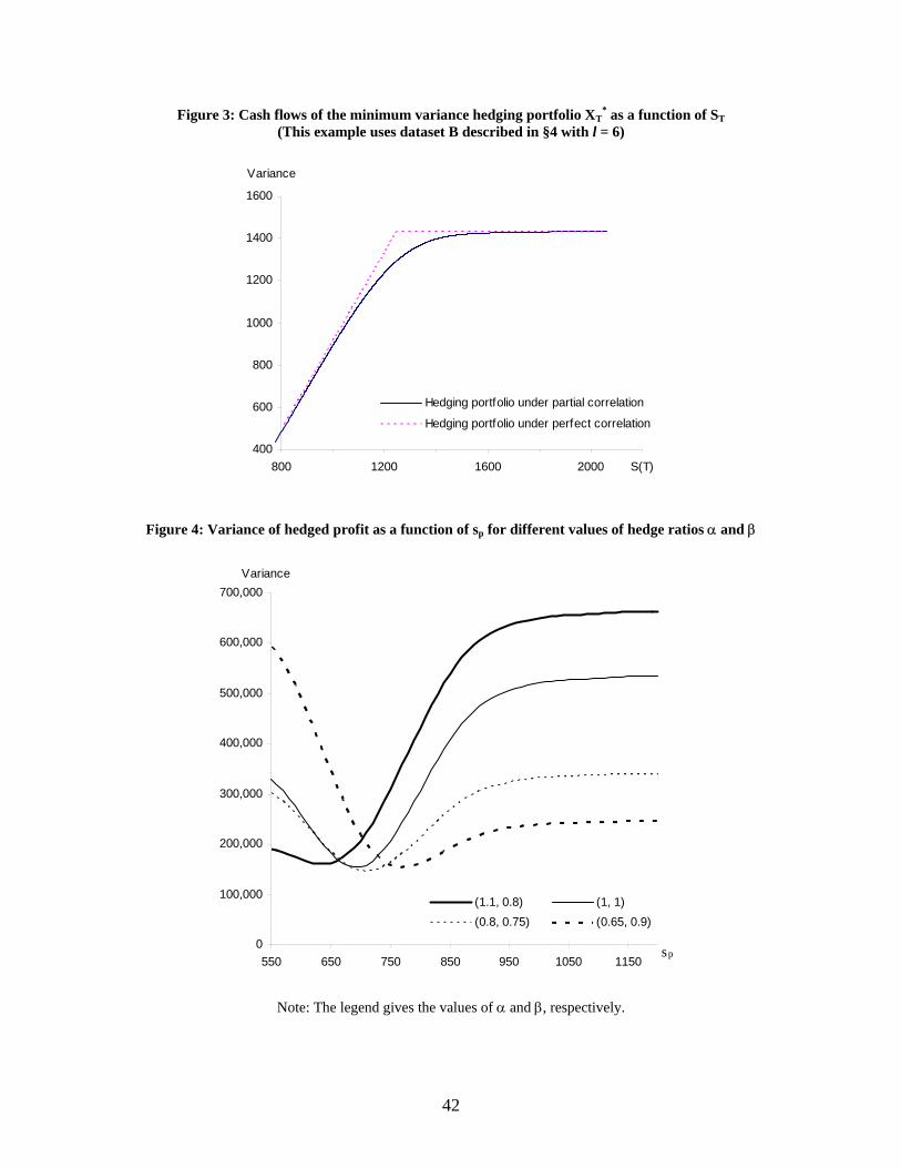
42

Figure 3: Cash flows of the minimum variance hedging portfolio XT* as a function of ST

(This example uses dataset B described in §4 with l = 6)

400

600

800

1000

1200

1400

1600

800 1200 1600 2000 S(T)

Variance

Hedging portfolio under partial correlation

Hedging portfolio under perfect correlation

Figure 4: Variance of hedged profit as a function of sp for different values of hedge ratios α and β

0

100,000

200,000

300,000

400,000

500,000

600,000

700,000

550 650 750 850 950 1050 1150

Variance

(1.1, 0.8) (1, 1)(0.8, 0.75) (0.65, 0.9)

sp

Note: The legend gives the values of α and β, respectively.

43

Figure 5: Q-Q Plot of the demand for item 1 shows that the demand distribution is skewed to the right

0

50

100

150

200

250

300

350

400

450

-3.5 -3 -2.5 -2 -1.5 -1 -0.5 0 0.5 1 1.5 2 2.5 3 3.5

Figure 6: Plot of β(ν) showing the bell-shaped curve

2( ) ( )/( )f AE Bβ ν = ν −

0lim ( ) 0ν→ β ν =

0 e ν

remains concave for 0 < ν < sp.

concave for small values of ν, convex for large values.