heft 251 alexander kissinger basin-scale site screening and
TRANSCRIPT
Heft 251 Alexander Kissinger
Basin-Scale Site Screening and
Investigation of Possible Impacts of
CO2 Storage on Subsurface Hydrosystems


Basin-Scale Site Screening and Investigation of Possible
Impacts of CO2 Storage on Subsurface Hydrosystems
von der Fakultät Bau- und Umweltingenieurwissenschaften der
Universität Stuttgart zur Erlangung der Würde eines
Doktor-Ingenieurs (Dr.-Ing.) genehmigte Abhandlung
vorgelegt von
Alexander Kissinger
aus Heilbronn
Hauptberichter: apl. Prof. Dr.-Ing. Holger Class
Mitberichter: Prof. Dr. Michael Kühn
Mitberichter: Prof. Dr.-Ing. Rainer Helmig
Tag der mündlichen Prüfung: 17.10.2016
Institut für Wasser- und Umweltsystemmodellierung der Universität Stuttgart
2016

Heft 251 Basin-Scale Site Screening and Investigation of Possible Impacts of CO2 Storage on Subsurface Hydrosystems
von Dr.-Ing. Alexander Kissinger
Eigenverlag des Instituts für Wasser- und Umweltsystemmodellierung der Universität Stuttgart
D93 Basin-Scale Site Screening and Investigation of Possible Impacts of
CO2 Storage on Subsurface Hydrosystems
Bibliografische Information der Deutschen Nationalbibliothek
Die Deutsche Nationalbibliothek verzeichnet diese Publikation in der Deutschen
Nationalbibliografie; detaillierte bibliografische Daten sind im Internet über
http://www.d-nb.de abrufbar
Kissinger, Alexander: Basin-Scale Site Screening and Investigation of Possible Impacts of CO2 Storage
on Subsurface Hydrosystems, Universität Stuttgart. - Stuttgart: Institut für Wasser- und Umweltsystemmodellierung, 2016
(Mitteilungen Institut für Wasser- und Umweltsystemmodellierung, Universität
Stuttgart: H. 251) Zugl.: Stuttgart, Univ., Diss., 2016 ISBN 978-3-942036-55-9 NE: Institut für Wasser- und Umweltsystemmodellierung <Stuttgart>: Mitteilungen
Gegen Vervielfältigung und Übersetzung bestehen keine Einwände, es wird lediglich um Quellenangabe gebeten. Herausgegeben 2016 vom Eigenverlag des Instituts für Wasser- und Umweltsystem-modellierung
Druck: Document Center S. Kästl, Ostfildern
Danksagung
Zuerst möchte ich mich beim Bundesministerium für Bildung und Forschung (BMBF) und beider Deutschen Forschungsgemeinschaft (DFG) bedanken, welche große Teile dieser Arbeit imRahmen des Forschungsprojekts CO2BRIM finanziell gefördert haben.Besonderer Dank gilt meinem Hauptberichter Holger Class für die große Unterstützung unddas mir entgegengebrachte Vertrauen. Er hat mich auf dem ganzen Weg von der Studienarbeit,über die Diplomarbeit bis hin zu meiner Promotion betreut und mir stets viele Freiräume beider Umsetzung meiner Arbeit gelassen. Sein fachlicher Input war dabei immer sehr wertvollund von seiner gelassenen und ruhigen Art Probleme anzugehen, konnte ich viel lernen. BeiRainer Helmig möchte ich mich, neben der Übernahme des Mitberichts, auch für viele lehr-und hilfreiche Diskussionen bedanken sowie für die einzigartige und sehr positive Stimmungam Lehrstuhl, die er maßgeblich zu verantworten hat. Michael Kühn möchte ich danken, dasser den Mitbericht übernommen hat und mich auch fachlich unterstützte.Mein Dank gilt auch den CO2BRIM Kollegen Stefan Knopf, Wilfried Konrad, Vera Noack undDirk Scheer. Die Arbeit mit ihnen hat mir sehr viel Spaß gemacht. Ich denke, wir verdienenwirklich das Prädikat interdisziplinär. Lena Mahl möchte ich zum einen danken, dass sie michwährend der Studien- und Diplomarbeit betreut hat und viel dazu beigetragen hat, dass ichmich für die Promotion hier entschieden habe. Zum anderen auch für die tolle Zeit im CO2 Büro.Bei Bernd Flemisch möchte ich mich vor allem dafür bedanken, wie er die DuMux Entwicklungvorantreibt und leitet. Es hat viel Spaß gemacht Teil des Entwicklerteams zu sein. ChristophGrüninger, Vishal Jambhekar und Emna Mejri möchte ich für die produktive Kelleratmosphäredanken. Pru Lawday und Maria Costa gebührt viel Dank für die Hilfe, die sie mir bei derBewältigung von verwaltungstechnischen Angelegenheiten geleistet haben. Ned Coltman dankeich für seine sprachlichen Korrekturen an der Arbeit und Simon Scholz und Marcel Wirth fürihre wertvollen Beiträge, welche aus ihren Bachelor-Arbeiten hervorgingen. Allen Kollegenaus der Arbeitsgruppe möchte ich für die tolle Atmosphäre hier am Lehrstuhl danken. Ichwerde immer gerne auf Veranstaltungen wie den Georgenhof (-burg), Lehrstuhlexkursionen,Weinproben, Karaokeabende, etc. zurückblicken.Weiterhin möchte ich der sog. Spalter-Gruppe danken, bestehend aus meinen Freunden LydiaSeitz, Tobias Mosthaf, Julian Mehne, Michael Sinsbeck und Johannes Hommel. Wenn ich beider Arbeit grübelte, halfen unsere gemeinsamen Mensagänge mich wieder auf andere Gedankenzu bringen. Meinen Eltern und meinem Bruder Thomas möchte ich für alles, was sie über dieJahre für mich getan haben, danken. Insbesondere meinem Bruder, der mich am Anfang desStudiums immer darin bestärkte diesen Weg zu gehen. Last and most möchte ich mich beimeiner Lebensgefährtin Melanie bedanken. Deine Unterstützung und Dein Rückhalt währendder letzten Jahre und vor allem in der Schlussphase der Promotion waren unheimlich wichtig.

Contents
List of Figures V
List of Tables XI
Notation XIII
Abstract XIX
Zusammenfassung XXIII
1. Introduction 11.1. Motivation and Aims . . . . . . . . . . . . . . . . . . . . . . . . . . . . . . . . 11.2. Literature Review . . . . . . . . . . . . . . . . . . . . . . . . . . . . . . . . . 5
1.2.1. Site-Screening Methods for CO2 Storage on the Basin Scale . . . . . . 51.2.2. Assessment of Large-Scale Brine Displacement due to CO2 Storage . . 7
1.3. Structure of this Thesis . . . . . . . . . . . . . . . . . . . . . . . . . . . . . . 9
2. Fundamentals of Porous-Media Flow 112.1. Spatial Scales and the Continuum Approach . . . . . . . . . . . . . . . . . . . 112.2. Local Thermodynamic Equilibrium . . . . . . . . . . . . . . . . . . . . . . . . 132.3. Properties of the Porous Medium . . . . . . . . . . . . . . . . . . . . . . . . . 13
2.3.1. Porosity and Compressibility of the Porous Medium . . . . . . . . . . 132.3.2. Permeability . . . . . . . . . . . . . . . . . . . . . . . . . . . . . . . . 14
2.4. Brine and CO2 . . . . . . . . . . . . . . . . . . . . . . . . . . . . . . . . . . . 152.4.1. Components and Phases . . . . . . . . . . . . . . . . . . . . . . . . . . 152.4.2. Mole and Mass Fractions . . . . . . . . . . . . . . . . . . . . . . . . . 162.4.3. Density . . . . . . . . . . . . . . . . . . . . . . . . . . . . . . . . . . . 162.4.4. Dynamic Viscosity . . . . . . . . . . . . . . . . . . . . . . . . . . . . . 17
2.5. Multi-Phase Flow . . . . . . . . . . . . . . . . . . . . . . . . . . . . . . . . . . 192.5.1. Saturation . . . . . . . . . . . . . . . . . . . . . . . . . . . . . . . . . . 192.5.2. Capillary Pressure . . . . . . . . . . . . . . . . . . . . . . . . . . . . . 192.5.3. Relative Permeability . . . . . . . . . . . . . . . . . . . . . . . . . . . 21
I

2.6. Transport Processes . . . . . . . . . . . . . . . . . . . . . . . . . . . . . . . . 232.6.1. Advection . . . . . . . . . . . . . . . . . . . . . . . . . . . . . . . . . . 232.6.2. Diffusion . . . . . . . . . . . . . . . . . . . . . . . . . . . . . . . . . . 242.6.3. Mechanical Dispersion . . . . . . . . . . . . . . . . . . . . . . . . . . . 24
2.7. Variable-Density Flow . . . . . . . . . . . . . . . . . . . . . . . . . . . . . . . 25
3. Model Concepts 273.1. Balance Equations . . . . . . . . . . . . . . . . . . . . . . . . . . . . . . . . . 27
3.1.1. Momentum Balance Equation . . . . . . . . . . . . . . . . . . . . . . . 273.1.2. Mass Balance Equations . . . . . . . . . . . . . . . . . . . . . . . . . . 28
3.2. Analytical Methods . . . . . . . . . . . . . . . . . . . . . . . . . . . . . . . . . 353.2.1. Analytical Solution for Estimating the Volumetric CO2 Storage Efficiency 363.2.2. Single-Phase Injection in a Multi-Layer System with a Fault Zone . . 37
3.3. Numerical Implementation . . . . . . . . . . . . . . . . . . . . . . . . . . . . . 423.3.1. Numerical Simulator DuMux . . . . . . . . . . . . . . . . . . . . . . . 423.3.2. Spatial Discretization: The Box-Method . . . . . . . . . . . . . . . . . 433.3.3. Temporal Discretization: The Implicit Euler Scheme . . . . . . . . . . 463.3.4. The Newton-Raphson Method . . . . . . . . . . . . . . . . . . . . . . 463.3.5. Fault-Zone Representation Using a Discrete-Fracture Approach . . . . 473.3.6. Infinite-Aquifer Boundary Conditions . . . . . . . . . . . . . . . . . . 52
4. Basin-Scale Screening for CO2 Storage Efficiency 554.1. The Gravitational Number as a Qualitative Indicator for Storage Efficiency . 564.2. Available Data . . . . . . . . . . . . . . . . . . . . . . . . . . . . . . . . . . . 594.3. Numerical Model Setup . . . . . . . . . . . . . . . . . . . . . . . . . . . . . . 624.4. Results . . . . . . . . . . . . . . . . . . . . . . . . . . . . . . . . . . . . . . . . 63
4.4.1. Basin-Scale Application of the Gravitational Number . . . . . . . . . . 644.4.2. Comparison of the Gr-Criterion and the Okwen-Method with Respect
to Storage Efficiency . . . . . . . . . . . . . . . . . . . . . . . . . . . . 644.4.3. Testing the Significance of the Gr-Criterion with Respect to Residual
Trapping . . . . . . . . . . . . . . . . . . . . . . . . . . . . . . . . . . 694.4.4. Testing the Significance of the Gr-Criterion with Respect to Porosity
and Reservoir Thickness . . . . . . . . . . . . . . . . . . . . . . . . . . 704.5. Discussion . . . . . . . . . . . . . . . . . . . . . . . . . . . . . . . . . . . . . . 734.6. Conclusion . . . . . . . . . . . . . . . . . . . . . . . . . . . . . . . . . . . . . 74
5. Large-Scale Investigation of Brine Displacement 775.1. Uncertainty Categorization and Brine Displacement . . . . . . . . . . . . . . 785.2. Available Data . . . . . . . . . . . . . . . . . . . . . . . . . . . . . . . . . . . 79
II

5.3. Numerical Model Setup . . . . . . . . . . . . . . . . . . . . . . . . . . . . . . 825.3.1. Boundary and Initial Conditions for the Numerical Models . . . . . . 835.3.2. Fault Zone Representation Using a Discrete-Fracture Model . . . . . . 85
5.4. Numerical Model Reliability . . . . . . . . . . . . . . . . . . . . . . . . . . . . 855.4.1. Large-Scale Pressure Propagation During Injection . . . . . . . . . . . 855.4.2. Upconing with Variable Brine Density: The Saltpool Experiment . . . 88
5.5. Results . . . . . . . . . . . . . . . . . . . . . . . . . . . . . . . . . . . . . . . . 925.5.1. Definition of Target Variables . . . . . . . . . . . . . . . . . . . . . . . 925.5.2. Scenario Uncertainty . . . . . . . . . . . . . . . . . . . . . . . . . . . . 945.5.3. Model Uncertainty (Recognized ignorance) . . . . . . . . . . . . . . . 104
5.6. Discussion . . . . . . . . . . . . . . . . . . . . . . . . . . . . . . . . . . . . . . 1125.7. Conclusion . . . . . . . . . . . . . . . . . . . . . . . . . . . . . . . . . . . . . 116
6. Summary and Outlook 1196.1. Summary . . . . . . . . . . . . . . . . . . . . . . . . . . . . . . . . . . . . . . 1196.2. Outlook . . . . . . . . . . . . . . . . . . . . . . . . . . . . . . . . . . . . . . . 124
Bibliography 129
A. Further Information for Simulations in Chapter 4 139
III

IV

List of Figures
2.1. A porous medium in the micro (left), and macro-scale perspective (right) (Nuske,2014). . . . . . . . . . . . . . . . . . . . . . . . . . . . . . . . . . . . . . . . . 11
2.2. The fluctuation of a physical property over the considered volume. The con-sideration as an REV is possible if fluctuations are sufficiently small. Figurefrom Helmig (1997), modified by (Nuske, 2014). . . . . . . . . . . . . . . . . . 12
2.3. The density of brine over temperature for different salinities (left) at a pressureof 100 bar. The density of CO2 over pressure for different temperatures (right). 17
2.4. The viscosity of brine over temperature for different salinities (left) at a pressureof 100 bar. The viscosity of CO2 over pressure for different temperatures (right). 18
2.5. Capillary pressure-saturation relationship for pe = 0.1 bar, λBC = 2.0, Srw =0.3, and Srn = 0.0. Note that the curve is regularized with a linear function atSw = 0.31 to avoid unrealistically high capillary pressures. . . . . . . . . . . . 20
2.6. Relative permeability-saturation relationship for λBC = 2.0, Srw = 0.3, andSrn = 0.0. . . . . . . . . . . . . . . . . . . . . . . . . . . . . . . . . . . . . . . 23
3.1. Injection of CO2 in a confined aquifer. The vertical pressure distribution isassumed hydrostatic for the sharp interface model. . . . . . . . . . . . . . . . 32
3.2. Multi-layer system with n aquifers coupled through a fault zone, modifiedafter Scholz (2014). The bottommost layer is the injection horizon. Each layeris split into two regions coupled through the fault zone. . . . . . . . . . . . . 38
3.3. Schematic overview of the solution procedure for the Zeidouni-Method, modifiedafter Scholz (2014). For numerically inverting the Laplace transform the Stehfestalgorithm is used (Stehfest, 1970). . . . . . . . . . . . . . . . . . . . . . . . . 41
3.4. Box constructed on a finite-element grid (left). Basis and weighting functionfor a node i (right). For 2D quadrilaterals the basis function is bilinear, and for3D cubes it is trilinear. Figure modified after Darcis (2012). . . . . . . . . . . 43
V
3.5. Grid with variable vertical discretization length and a fault zone shown in red.Note that the width of the fault zone (wij) may be greater than the verticaldiscretization length. The bottom shows a zoom on a fracture element face,containing the nodes i and j from the above grid, in x and y direction. Thefault-zone width wij is an input parameter of the fracture model. dij is thedistance between nodes i and j, and hij is the distance between the midpointof the line connecting nodes i and j and the center of the element face. Bothdij and hij are calculated from the geometry of the element face. . . . . . . . 48
3.6. An inner domain within the red frame is surrounded by an outer domain withradius Ro. . . . . . . . . . . . . . . . . . . . . . . . . . . . . . . . . . . . . . . 53
4.1. Unpublished depth grid for the base of the Upper Buntsandstein (equivalentto the top of the Middle Buntsandstein) with depths recorded in meters belowmean sea level (bmsl). Figure from Kissinger et al. (2014). . . . . . . . . . . . 59
4.2. The interpolated distribution of the geothermal gradient for the area of interest(based on (LIAG, 2012)). Figure from Kissinger et al. (2014). . . . . . . . . 60
4.3. The CO2 density as a function of pressure and temperature (top left), the CO2
viscosity as a function of pressure and temperature (top right), the brine densityas a function of salinity and temperature (bottom left) and the brine viscosityas a function of salinity and temperature (bottom right). The red points arethe data points from the database. They are not plotted with the brine density(bottom left) as they are a function of pressure, salinity and temperature andwould therefore not fit on the brine density surface shown here. Figure modifiedafter Kissinger et al. (2014). . . . . . . . . . . . . . . . . . . . . . . . . . . . . 62
4.4. Schematic setup of the model domain for the numerical simulations. Dueto symmetry reasons only a small part of the radially symmetric problem issimulated. Figure from Kissinger et al. (2014). . . . . . . . . . . . . . . . . . 63
4.5. Distribution of Gr for the Middle Buntsandstein rock unit in the North GermanBasin. The numbers refer to the areas selected in Sec. 4.4.4 (Area 1 = low Gr,Area 2 = medium Gr, Area 3 = high Gr). Figure from Kissinger et al. (2014). 65
4.6. Left: Simulation results in terms of storage efficiency (SE) for 49 data pointsover Gr. Right: The same simulation results plotted over storage efficiencyobtained from the Okwen-Method using Eq. 3.37 and 4.7. Figure modifiedafter Kissinger et al. (2014). . . . . . . . . . . . . . . . . . . . . . . . . . . . . 67
4.7. Left: Simulation results for two injection rates (0.1 and 1.0Mt per year) plottedover Gr. Note the logarithmic scaling of Gr. Right: The same simulationresults plotted over storage efficiency (SE) obtained from the Okwen-Methodusing Eq. 3.37 and 4.7. Figure modified after Kissinger et al. (2014). . . . . . 68
VI

4.8. Comparison of storage efficiency (SE) and the residually trapped CO2 mass (alsogiven in terms of storage efficiency, i.e. kg/m2). Figure modified after Kissingeret al. (2014). . . . . . . . . . . . . . . . . . . . . . . . . . . . . . . . . . . . . 70
4.9. Left: Storage efficiency over Gr. The cross marker represents the mean storageefficiency and the bars indicate the standard deviation. Right: Mean storageefficiency for the three areas with constant Gr for all areas (black curve) andarea-specific Gr (red curve). Note: the three means for the area-specific case(red cross marker) on the right plot are identical to the three means on the leftplot (red cross marker). Figure modified after Kissinger et al. (2014). . . . . . 72
5.1. Levels of uncertainty after Walker et al. (2003), modified by Walter et al. (2012). 785.2. Top of the Solling injection horizon discontinuous where the salt wall penetrates
the layer. The top of the Zechstein salt is displayed with a blue mesh. Theinjection point at the flank of the anticlinal structure in about 1651m depth isprojected on top of the Solling injection horizon. Vertical exaggeration is 2:1.Figure from Kissinger et al. (2017). . . . . . . . . . . . . . . . . . . . . . . . . 79
5.3. Top of the Rupelian clay barrier with discontinuities where Cretaceous sedimentspenetrate the Rupelian clay barrier. The top of the Cretaceous is displayed asblue mesh. Vertical exaggeration is 2:1. Figure from Kissinger et al. (2017). . 80
5.4. Top view on the groundwater table. The rivers are highlighted in blue. Theelevation values are normalized to the minimum elevation of the groundwatertable. Figure from Kissinger et al. (2017). . . . . . . . . . . . . . . . . . . . . 81
5.5. Perspective view on the 3D geological model with zoom in on the anticlinalstructure showing the mesh of the 3D volume model. Vertical exaggeration2:1. Here Quaternary 1 and 2 are combined in the Quaternary layer. Figurefrom Kissinger et al. (2017). . . . . . . . . . . . . . . . . . . . . . . . . . . . . 81
5.6. Boundary and initial conditions of the domain. Also shown is the position ofthe fault zone situated on the flank of the salt wall in red. . . . . . . . . . . . 83
5.7. a) Cross-section of the domain showing the lateral and top boundary conditionsas well as the injection well and the fault zone (modified after Scholz (2014)).b) Top view on the upper aquifer showing the inner domain (30 km× 25 km)in blue and the domain extension with an outer radius of 100 km in red. Dueto the symmetry of the line connecting the injection and the fault zone onlyhalf of the domain is simulated. . . . . . . . . . . . . . . . . . . . . . . . . . . 86
5.8. Comparison of domain radii for 50, 100 and 150 km. Left: Neumann case withthe upper aquifer closed on top. Right: Dirichlet case where the top aquiferhas a constant pressure (very large diffusivity). . . . . . . . . . . . . . . . . . 87
VII
5.9. Comparison of different horizontal discretization lengths for 150, 300 and 450 m.Left: Neumann case with the upper aquifer closed on top. Right: Dirichletcase where the top aquifer has a constant pressure (very large diffusivity). . . 88
5.10. Setup of the saltpool benchmark. . . . . . . . . . . . . . . . . . . . . . . . . . 895.11. a) and b): diagonal vertical cross-sections between inlet and outlet showing
the salinity after 9000 s. Also shown are the 10% and 50% isolines for the low(0.01) and high (0.1) salinity case. c) and d): salinity at outlet over time forthe low (0.01) and high (0.1) salinity case, with 503, 1003 and 1253 elements. 91
5.12. a) Top view on the Rupelian clay barrier. Also shown are the two hydrogeologicalwindows in the Rupelian clay barrier and the salt wall piercing through thebarrier layer. The fault zone on the salt wall is is highlighted in red. b) showsa cross-section (vertical exaggeration 4:1) along line A-B with approximatelocations of the injection point (IP) and the two measurement points for pressure(M1 and M2). . . . . . . . . . . . . . . . . . . . . . . . . . . . . . . . . . . . . 93
5.13. (a): Initial salt distribution for the reference scenario before the initializationrun along the cross-section shown in Fig. 5.12 (vertical exaggeration 4:1).(b): Salt distribution for the reference scenario after an initialization run of300 000 years. Six concentration isolines are shown which correspond to theentries in the legend (0.01, 0.1, 1, 10, 100 and 300). The permeability of thedifferent layers is also shown. Please note the logarithmic scale of concentrationand permeability. . . . . . . . . . . . . . . . . . . . . . . . . . . . . . . . . . . 96
5.14. Top row: View on top of the Rupelian clay barrier for three different scenarioslow, medium and high with increasing initial salt gradients. The results show thesalt concentration increase after 50 years of injection. Concentration increasesbelow 0.01 g/L are not shown. Bottom row: View on top of the Post-Rupelianfor the three scenarios. Also see Fig. 5.12 for orientation. Note the differentscales for the top and bottom row. . . . . . . . . . . . . . . . . . . . . . . . . 97
5.15. Total salt flow into target aquifers (top left) over the injection and post-injection period split into salt flow over fault zone (top right), salt flow overhydrogeological windows (bottom left) and salt flow over the intact Rupelianclay barrier (bottom right). . . . . . . . . . . . . . . . . . . . . . . . . . . . . 98
5.16. The cumulative salt flow for a period of 100 years (injection + post injection)into the Tertiary Post-Rupelian layer (a), Quaternary 2 layer (b) and Quaternary1 layer (c) with and without injection. The scenario numbers along with shortexplanations of the varied parameters are given in (d). . . . . . . . . . . . . . 99
5.17. Left: Total mass flow into the target aquifers normalized by the injection rate.Right: Mass flow over fault zone into the target aquifers. . . . . . . . . . . . 100
VIII
5.18. Mass flow normalized by the brine injection rate into the target aquifers, fordifferent permeabilites of the Upper Buntsandstein barrier. The upper rightscenario with a permeability of 1× 10⁻¹⁸ m2 corresponds to the reference scenario.101
5.19. Maximum mass flow reached after 50 years of injection normalized by thebrine injection rate into the target aquifers over the fault zone permeability,for two different permeabilites of the Upper Buntsandstein barrier. Left: Highbarrier permeability, high diffuse migration over barrier; right: Low barrierpermeability, high focused migration over fault zone. . . . . . . . . . . . . . . 102
5.20. Left: Volumetric flow normalized by injection rate into target aquifers throughthe fault zone. Right: Salt flow into target aquifers through fault zone. . . . 103
5.21. Top: Volume flow over time into the target aquifers for the 1p1c and the 1p2cmodel. Bottom: Pressure increase due to injection at M1 and M2. . . . . . . 105
5.22. Volume flow over time into the target aquifers for the 2p3c and the 1p2c model.1065.23. Cross-section of the complex and generic geometry (vertical exaggeration 4:1)
along the same cross-section, as shown in Fig. 5.12. . . . . . . . . . . . . . . . 1075.24. Volume flow normalized by the injection rate over time into the target aquifers
for the generic and the complex model. . . . . . . . . . . . . . . . . . . . . . . 1085.25. Model setup for the Zeidouni-Method with two permeable layers (injection
horizon and intermediate aquifers) and the target aquifers with infinite diffusivity.1105.26. Top row: Total volume flow into target aquifers (left) and volume flow over fault
zone (right) for an Upper Buntsandstein barrier permeability of 1× 10⁻¹⁸ m2.Bottom row: Total volume flow into target aquifers (left) and volume flowover fault zone (right) for an Upper Buntsandstein barrier permeability of1× 10−20 m2. Also shown in the right figure is the Zeidouni-Method for thecase of a high injection horizon diffusivity. . . . . . . . . . . . . . . . . . . . . 111
IX

X

List of Tables
3.1. List of fully discretized equations. Note that in this work the 2p model is notused in combination with the fracture module, hence the equations for the 2pmodel only account for matrix flow. The matrix and fracture weighting factors(Wm and Wf ) are only implemented for the component balance equations ofsalt in the 1p2c and 2p3c model. . . . . . . . . . . . . . . . . . . . . . . . . . 49
3.1. List of fully discretized equations. Note that in this work the 2p model is notused in combination with the fracture module, hence the equations for the 2pmodel only account for matrix flow. The matrix and fracture weighting factors(Wm and Wf ) are only implemented for the component balance equations ofsalt in the 1p2c and 2p3c model. . . . . . . . . . . . . . . . . . . . . . . . . . 50
3.1. List of fully discretized equations. Note that in this work the 2p model is notused in combination with the fracture module, hence the equations for the 2pmodel only account for matrix flow. The matrix and fracture weighting factors(Wm and Wf ) are only implemented for the component balance equations ofsalt in the 1p2c and 2p3c model. . . . . . . . . . . . . . . . . . . . . . . . . . 51
4.1. The initial fluid properties of seven different data points as well as Gr and thestorage efficiency obtained from the simulations. . . . . . . . . . . . . . . . . 66
4.2. The characteristics of the three different areas. Note that for Area 1 and 3 thereare only ranges of a minimum and maximum value for porosity and thickness.For Area 2 the data points are listed in the the appendix in Table A.1. Thevalues for pressure, temperature, salinity and Gr are the mean values for eacharea and are used as initial conditions for the simulations. . . . . . . . . . . . 71
5.1. Properties of the model layers according to Larue (2010); Reutter (2011);Schäfer et al. (2011); Noack et al. (2013). . . . . . . . . . . . . . . . . . . . . 82
5.2. Input parameters for the analytical and the numerical model. ∗ denotes param-eters only relevant for the numerical simulation. . . . . . . . . . . . . . . . . . 87
5.3. Input parameters for the saltpool benchmark as given in Oswald and Kinzelbach(2004). . . . . . . . . . . . . . . . . . . . . . . . . . . . . . . . . . . . . . . . 90
XI
5.4. List of parameters for the 1p2c model for the reference scenario. The two-phaseflow specific parameters are additionally required for the 2p3c model. . . . . . 94
5.5. Averaged values for the permeability, porosity, viscosity and diffusivity of theinjection horizon and the intermediate aquifer for the Zeidouni-Method. . . . 109
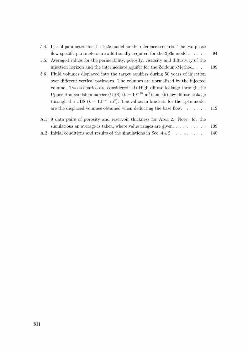
5.6. Fluid volumes displaced into the target aquifers during 50 years of injectionover different vertical pathways. The volumes are normalized by the injectedvolume. Two scenarios are considered: (i) High diffuse leakage through theUpper Buntsandstein barrier (UBS) (k = 10−18 m2) and (ii) low diffuse leakagethrough the UBS (k = 10−20 m2). The values in brackets for the 1p1c modelare the displaced volumes obtained when deducting the base flow. . . . . . . 112
A.1. 9 data pairs of porosity and reservoir thickness for Area 2. Note: for thesimulations an average is taken, where value ranges are given. . . . . . . . . . 139
A.2. Initial conditions and results of the simulations in Sec. 4.4.2. . . . . . . . . . 140
XII
Notation
The following table shows the significant symbols used in this work. Local notations areexplained in the text.
Symbol Definition Dimension
Greek Letters:
α Solute expansion coefficient -αl Longitudinal dispersivity mαt Transversal dispersivity mβ Product of parameters that require upwinding m2 s−1
Γ Dimensionless gravitational number -ΓG Variable of integration for domain boundary m2
ΓVi Variable of integration for boundary of finite volumeor box
m2
ε Mass balance error kg or mol s-1
η Dimensionless space -θ Weighting coefficient (0 ≤ θ ≤ 1) for temporal dis-
cretization scheme-
λ Mobility ratio λ = λnλw
-λα Moliltity of phase α, λα = krα
µαPa−1 s−1
λBC Brooks and Corey shape parameter -λt Total moliltity λt = λn + λw Pa−1 s−1
% Mass density kgm−3
%α Mass density of phase α kgm−3
%mα Molar density of phase α molm−3
µ Dynamic viscosity Pa sµα Dynamic viscosity of phase α Pa s
XIII
τ Dimensionless time -φ Effective Porosity -φdp Drainable porosity -χ Ratio of dimensionless time and space, χ = η
τ -
Latin Letters:
a Distance between fault zone and injection well mAα Cross-sectional area of phase α m2
AIP Area of sub-control volume face at integration pointIP
m2
Cs Compressibility of the solid matrix Pa−1
Ct Total compressibility of the fluid and the solid matrix Pa−1
C Dimensionless factor C = krnfw -Ca Dimensionless capillary number -d Characteristic grain diameter md10 Characteristic grain diameter whose size exceeds 10%
of the other diameters by weightm
dij Distance between nodes i and j mDdisp Mechanical dispersion tensor m2 s−1
Dκm Molecular diffusion of component κ m2 s−1
Dκpm Effective porous medium diffusion of component κ m2 s−1
Dj Diffusivity of aquifer j, Dj = kµwφCt
m2 s−1
E Volumetric CO2 stroage efficiency -f Flux vector kg or mol s-1m-2
fa Advective flux vector Nm−1
fd Diffusive flux vector kg or mol s-1m-2
ff Fracture flux vector kg or mol s-1m-2
fα Fractional-flow function of phase α, fα = λαλt
-g Gravity acceleration vector m s−2
g Scalar gravity acceleration g = 9.81 ms−2
G Model domain m3
Gr Dimensionless gravitational number -h Height of the CO2 front mh′ Dimensionless height of the CO2 front -
XIV
hij Distance from element center to midpoint of edge con-necting nodes i and j
m
H Aquifer thickness mK Intrinsic permeability tensor m2
k Scalar permeability m2
kf Scalar permeability of fracture m2
kfh,j Horizontal fault permeability in aquifer j m2
kfv,j Vertical fault permeability in aquifer j m2
krα Relative permeability of phase α -lcr Characteristic length mLj Distance between midpoints of aquifers j and j + 1 mMα Average molar weight of a phase α kgmol−1
Mκ Molar weight of a component κ kgmol−1
n Unit normal vector of sub-control volume face -nij Unit normal vector of sub-control volume face between
node i and j-
nIP Unit normal vector of sub-control volume face at inte-gration point IP
-
N Number nodes in a grid -Ni Linear basis function, Ni = Ni(x) -p Pressure Papα Pressure of phase α Papc Capillary pressure Pape Entry pressure Papc Dimensionless capillary pressure -pcr Characteristic pressure Pa∆pj1 Pressure change in aquifer j region 1 Pa∆pj2 Pressure change in aquifer j region 2 Paq Source or sink term kg or mol s-1m-3
qα Source or sink term of phase α kg or mol s-1m-3
qκ Source or sink term of component κ kg or mol s-1m-3
qt Total source or sink term of kg or mol s-1m-3
Qleakage Volumetric leakage rate m3
Qwell Volumetric injection rate m3
r Residual vector of whole domain kg or mol s-1
r Radial coordinate mri Residual at node i kg or mol s-1
XV
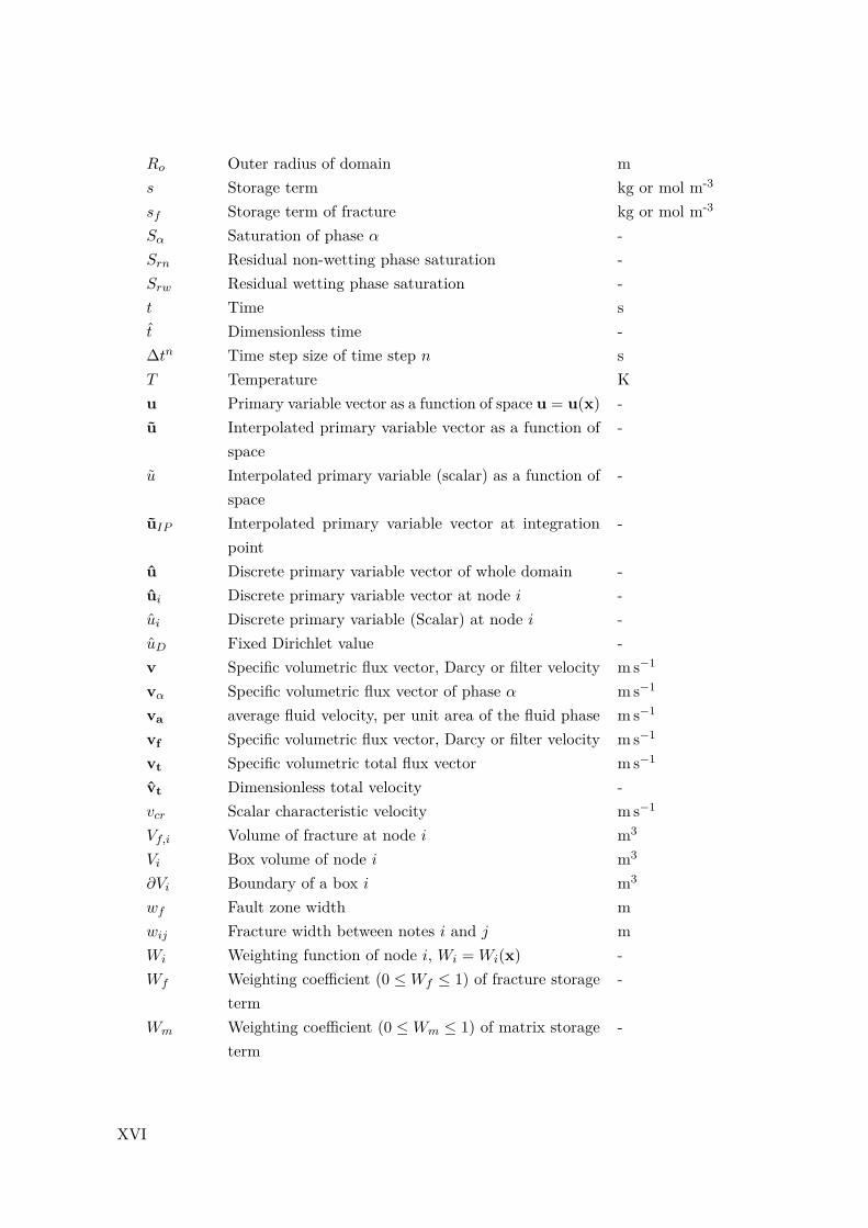
Ro Outer radius of domain ms Storage term kg or mol m-3
sf Storage term of fracture kg or mol m-3
Sα Saturation of phase α -Srn Residual non-wetting phase saturation -Srw Residual wetting phase saturation -t Time st Dimensionless time -∆tn Time step size of time step n sT Temperature Ku Primary variable vector as a function of space u = u(x) -u Interpolated primary variable vector as a function of
space-
u Interpolated primary variable (scalar) as a function ofspace
-
uIP Interpolated primary variable vector at integrationpoint
-
u Discrete primary variable vector of whole domain -ui Discrete primary variable vector at node i -ui Discrete primary variable (Scalar) at node i -uD Fixed Dirichlet value -v Specific volumetric flux vector, Darcy or filter velocity m s−1
vα Specific volumetric flux vector of phase α ms−1
va average fluid velocity, per unit area of the fluid phase m s−1
vf Specific volumetric flux vector, Darcy or filter velocity m s−1
vt Specific volumetric total flux vector m s−1
vt Dimensionless total velocity -vcr Scalar characteristic velocity m s−1
Vf,i Volume of fracture at node i m3
Vi Box volume of node i m3
∂Vi Boundary of a box i m3
wf Fault zone width mwij Fracture width between notes i and j mWi Weighting function of node i, Wi = Wi(x) -Wf Weighting coefficient (0 ≤Wf ≤ 1) of fracture storage
term-
Wm Weighting coefficient (0 ≤Wm ≤ 1) of matrix storageterm
-
XVI
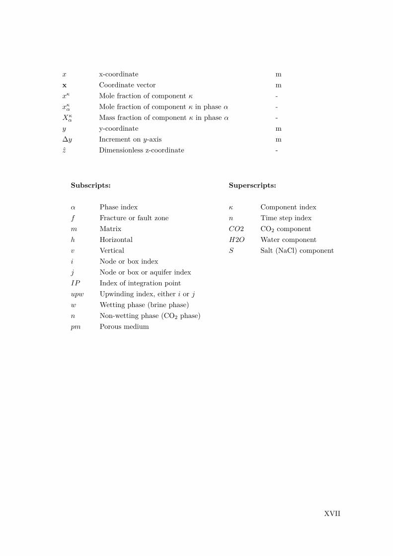
x x-coordinate mx Coordinate vector mxκ Mole fraction of component κ -xκα Mole fraction of component κ in phase α -Xκα Mass fraction of component κ in phase α -
y y-coordinate m∆y Increment on y-axis mz Dimensionless z-coordinate -
Subscripts:
α Phase indexf Fracture or fault zonem Matrixh Horizontalv Verticali Node or box indexj Node or box or aquifer indexIP Index of integration pointupw Upwinding index, either i or jw Wetting phase (brine phase)n Non-wetting phase (CO2 phase)pm Porous medium
Superscripts:
κ Component indexn Time step indexCO2 CO2 componentH2O Water componentS Salt (NaCl) component
XVII

XVIII
Abstract
Carbon Dioxide, Capture and Storage (CCS) is considered to be a cost-effective technologyfor mitigating climate change in the near future. A necessary requirement for a successfulimplementation of CCS is the public acceptance of the technology. The affected public needsto be aware of, and accept the risks that are associated with the subsurface storage of CO2.This demands the use of transparent and comprehensible criteria in a site-selection andcharacterization process.Such a process comprises several levels. The first level should be a basin-scale screening usingdifferent criteria with the aim of identifying favorable areas and sites for CO2 storage. Oncepotential sites have been identified, an exploration should be carried out to obtain site-specificdata. The next step should comprise a site-specific investigation of the risks associated withCO2 storage, covering such risks as the leakage of CO2 from the reservoir and the risk ofsaltwater intrusion in freshwater aquifers. This work deals with two aspects of such a multi-levelsite-selection and characterization process. The first aspect is related to a basin-scale screeningmethod, allowing for a qualitative ranking of different areas with respect to storage efficiency.The second aspect investigates the displacement of resident brine during the injection ofCO2, on the basis of a realistic, but not real large-scale site in the North German Basin. Forboth aspects, the relevant processes and parameters are analyzed, and models with varyingcomplexity are compared for the target variables of interest.
Basin-Scale Screening for CO2 Storage Efficiency An important requirement for a screeningmethod is a low computational demand, as the screening has to be carried out over a largearea. For this purpose, the dimensionless gravitational number (Gr), which has a negligiblecomputational demand, is considered here as a screening criterion. Gr relates gravitationalforces to viscous forces during CO2 injection, and is therefore a qualitative indicator of howefficient a reservoir can be used (i.e. storage efficiency). The basin-scale database available inthis work comprises regionalized data for depth, temperature conditions, and salt concentrationsin the Middle Buntsandstein rock unit of the North German Basin. These data are sufficientto determine the initial fluid properties (viscosities and densities) of brine and CO2. However,other relevant parameters like the permeability, the porosity, and the reservoir thickness are
XIX

not regionalized on the basin scale. Gr is therefore calculated based on the fluid properties atevery data point of the database. The Gr-criterion allows only for a qualitative ranking ofdifferent sites, therefore numerical simulations are performed to test if there is a significantinfluence of the varying fluid properties on storage efficiency. Additionally, the influence ofthe parameters porosity and reservoir thickness, for which data are only available in selectedareas, is compared to the influence of the varying fluid properties in these areas. The resultssuggest, that the influence of the fluid properties on the storage efficiency is notable but lessimportant, than that of the parameters porosity and reservoir thickness. Still, the influence ofthe fluid properties can be in the same range as the other two parameters.Additionally, the Gr-criterion is compared to the Okwen-Method, which is an analytical solutionfor estimating the storage efficiency. The main finding is, that both methods show an acceptablequalitative agreement with the simulation results for large parts of the considered range ofdepth, temperature conditions, and salt concentrations found in the Middle Buntsandsteinrock unit.To summarize, a screening method, such as the Gr-criterion or the Okwen-Method based onthe available database of depth, temperature conditions, and salt concentrations can providevaluable information for identifying suitable areas for CO2 storage. However, it becomes clearthat these criteria can only be part of a larger set of criteria that have to evaluated.
Large-Scale Investigation of Brine Displacement Brine displacement is considered to be apotential risk of CO2 storage. A site selection process should therefore include a phase wherethe fate of the brine displaced by the injected CO2 is investigated. For this purpose, differentnumerical and analytical models exist. This work investigates brine displacement in a realistic(but not real) CO2 storage site in the North German Basin.The geological model comprises, besides the injection horizon and its surrounding layers, thecomplete overburden up to the shallow freshwater aquifers. It therefore fully couples flowbetween deep and shallow layers. Several characteristics of the North German Basin areincluded in the geological model, such as a salt wall, which penetrates all layers up to theshallow freshwater aquifers, and the Rupelian clay barrier, which separates saltwater fromfreshwater aquifers. The Rupelian clay barrier is discontinuous at several locations, so-calledhydrogeological windows, which allow for an exchange between saltwater and freshwater. Thesecond important barrier in the geological model is the Upper Buntsandstein barrier, which isthe main barrier preventing the CO2 from migrating upwards. It is situated approximately1300m below the Rupelian clay barrier. A conservative assumption is made by assuminga permeable fault zone, at the flank of the salt wall. This fault zone directly connects theinjection horizon to the freshwater aquifers, which are, in this work, referred to as targetaquifers.
XX

In a scenario study, different components of the geological model are varied, not in a statisticalsense, but on the entire range of plausible values, thereby creating a span of possible results.This allows, to some extent, a generalization of the conclusions drawn here to other sites,at least within the North German Basin. The results presented in this work show first andforemost that notable, in the sense of non-negligible, increases in the salt concentration in thetarget aquifers are locally constrained to regions, where initially elevated concentrations arepresent prior to the injection, and where permeabilities are high enough to support sufficientflow (i.e. at the fault zone and the hydrogeological windows). Hence, the quality of theprediction of concentration changes strongly depends on how well the initial salt distribution isknown. Another important parameter is the permeability of the Upper Buntsandstein barrier.It has a strong influence on the type of brine displacement, which can either be diffuse acrossthe barrier or focused over the fault zone.In a further study, models with varying complexity are compared. More complex modelswill increase the computational demand and require more data. In general, hydrogeologicaldata are highly uncertain, therefore a risk analysis may require many realizations of a model(for example Monte-Carlo simulations). To limit the computational demand, while still beingable to handle the uncertainties in the data, requires the use of simplified models. The mainaim of this model comparison is to reduce the model uncertainty, by investigating the effectsof the different model simplifications. The analysis on model simplification shows that thelevel, to which the complexity of a model can be reduced, depends on the target variable ofinterest. For example, when considering the volumetric leakage rate into the target aquifers asa target variable most of the model simplifications compared in this work show an acceptableagreement. However, when considering the pressure-buildup as a target variable the agreementbetween some of the considered model simplifications significantly worsens. The agreementbetween the different models has to be evaluated bearing in mind the uncertainty of thehydrogeological parameters, whose impact is expected to be much greater than the impact ofmost of the model simplifications treated here.Overall, the analysis on brine displacement presented in this work, will help in the design ofeffective and efficient large scale models. A possible application could be a basin-scale modelof the North German Basin considering multiple CO2 injections.
XXI

XXII
Zusammenfassung
Die CO2-Abscheidung und -Speicherung (CCS, engl. Carbon Dioxide Capture and Stora-ge) wird als kosteneffiziente Technologie zur Minderung der anthropogenen Emissionen desTreibhausgases CO2 in die Atmosphäre angesehen. Die CCS-Technologie könnte somit einenwichtigen Beitrag zur Abschwächung der Folgen des Klimawandels in naher Zukunft leisten.Eine erfolgreiche Umsetzung der CCS-Technologie, in einem klimarelevanten Maßstab, hängtstark von deren öffentlicher Akzeptanz ab. Die Risiken für Mensch und Umwelt, welche mitder unterirdischen Speicherung von CO2 einhergehen, sollten daher offen kommuniziert undvon einer betroffenen Öffentlichkeit akzeptiert werden. Deshalb ist es notwendig bei der Suchenach geeigneten Standorten transparente und nachvollziehbare Auswahlkriterien einzusetzen.Die Standortauswahl sollte in mehreren Stufen verlaufen. Zuerst können, durch ein großflä-chiges Screening, anhand verschiedener Kriterien, geeignete Gebiete für die CO2-Speicherungidentifiziert werden. Nach der Identifizierung von potentiellen Standorten, kann eine Erkun-dung folgen, mit deren Hilfe standortspezifische Daten erhoben werden können. In einemweiteren Schritt sollte eine standortspezifische Risikoanalyse durchgeführt werden, z.B. zumRisiko der Migration von CO2 aus dem Speicherhorizont oder der Beeinträchtigung von Süß-wasseraquiferen durch verdrängtes Salzwasser. Diese Arbeit befasst sich mit zwei Aspektendieser mehrstufigen Standortauswahl. Der erste Aspekt beschreibt eine Screening-Methode zurgroßflächigen Untersuchung von geeigneten Gebieten in Bezug auf die CO2-Speichereffizienz,wodurch eine qualitative Einteilung dieser Gebiete ermöglicht wird. Im zweiten Aspekt wirddie Verdrängung der im Injektionshorizont vorhandenen Sole anhand eines realistischen, jedochnicht realen Standorts innerhalb des Norddeutschen Beckens untersucht. Für beide in dieserArbeit behandelten Aspekte werden Modelle mit unterschiedlicher Komplexität sowie dierelevanten physikalischen Prozesse und Parameter untersucht.
Großflächiges Screening in Bezug auf die CO2-Speichereffizienz Eine wichtige Vorausset-zung für eine Screening-Methode ist ein möglichst geringer Rechenaufwand, da große Gebieteschnell und effektiv evaluiert werden müssen. Aus diesem Grund wird hier die Eignung derdimensionslosen Gravitationszahl (Gr-Zahl), die mit vernachlässigbar kleinem Rechenaufwand
XXIII

bestimmt werden kann, als Screening-Kriterium untersucht. Die Gr-Zahl beschreibt das Ver-hältnis von Gravitationskräften zu viskosen Kräften, während der CO2-Injektion und ist somitals qualitativer Indikator, für eine effiziente Ausnutzung des betrachteten Reservoirs (Spei-chereffizienz), einsetzbar. Die Datenbasis, welche für diese Analyse zur Verfügung steht, umfasstregionalisierte Tiefen-, Temperatur- und Salzkonzentrationsdaten des Mittleren Buntsandsteinsim Norddeutschen Becken. Die Datenbasis ist somit ausreichend zur Bestimmung der im Injek-tionshorizont vorliegenden Fluideigenschaften (Viskosität und Dichte) von Sole und CO2. DieDatenbasis für den Mittleren Buntsandstein enthält jedoch keine regionalisierten Daten zu denPermeabilitäten, den Porositäten und den Formationsmächtigkeiten. Die Gr-Zahl wird deshalbnur unter Berücksichtigung der Fluideigenschaften bestimmt. Die Bestimmung wird für jedenDatenpunkt der Datenbasis durchgeführt, so dass die Gr-Zahl regionalisiert vorliegt. Da dasGr-Kriterium nur eine qualitative Differenzierung von verschiedenen Gebieten zulässt, werdenzusätzlich numerische Simulationen durchgeführt, um zu prüfen, ob die Variabilität in denregionalisierten Fluideigenschaften einen großen Einfluss auf die Speichereffizienz hat. Hierbeiwird auch der Einfluss von Parametern wie der Porosität und der Formationsmächtigkeituntersucht, für die Daten nur in ausgewählten Gebieten verfügbar sind. Die Simulationsergeb-nisse zeigen, dass variable Fluideigenschaften, basierend auf den regionalisierten Daten vonTiefe, Temperatur und Salzkonzentrationen, eine wichtige Rolle spielen. Ihr Einfluss ist jedochden Parametern Porosität und Formationsmächtigkeit untergeordnet, kann aber auch von dergleichen Größenordnung sein.Weiterhin wurde das Gr-Kriterium mit der Okwen-Methode verglichen. Die Okwen-Methodeist eine analytische Lösung zur Bestimmung der Speichereffizienz. Die zentrale Schlussfolge-rung dieses Vergleichs ist, dass beide Methoden eine passable qualitative Übereinstimmungmit den durchgeführten Simulationen zeigen für weite Teile der im Mittleren Buntsandsteinvorliegenden Tiefen-, Temperatur- und Salzkonzentrationsdaten.Zusammenfassend lässt sich zu dieser Untersuchung feststellen, dass sowohl das Gr-Kriteriumals auch die Okwen-Methode wertvolle Informationen zur Identifizierung von geeignetenGebieten für die CO2-Speicherung liefern können, ausgehend von der verwendeten Datenba-sis. Jedoch müssen beide Methoden Teil eines größeren Kriterienkatalogs sein, welcher zurIdentifizierung von geeigneten Gebieten eingesetzt wird.
Großskalige Untersuchung der Sole-Migration an einem realistischen Standortmodell DieVerdrängung von Sole durch die Injektion von CO2 ist eines der Risiken, welches mit derCO2-Speicherung assoziiert wird. Aus diesem Grund sollten bei der Wahl eines geeignetenStandortes die Auswirkungen der Sole-Verdrängung untersucht werden. Hierfür stehen verschie-dene analytische und numerische Modelle zur Verfügung. In dieser Arbeit wird die Verdrängungvon Sole anhand eines realistischen, jedoch nicht realen Standorts zur CO2-Speicherung im
XXIV
Norddeutschen Becken untersucht.Das hierfür verwendete geologische Modell umfasst, neben dem Injektionshorizont, das kom-plette Deckgebirge bis zu den oberflächennahen Süßwasseraquiferen. Somit ist die Grundwas-serströmung zwischen tiefen und oberflächennahen Schichten voll gekoppelt. Das geologischeModell enthält weiterhin für das Norddeutsche Becken typische Merkmale, wie z.B. einenSalzwall, welcher alle Schichten bis zu den oberflächennahen Süßwasseraquiferen durchbrichtoder die Barriereschicht Rupelton, welche Süß- und Salzwasseraquifere voneinander trennt. DerRupelton ist an einigen Stellen unterbrochen, sog. Rupelfehlstellen, welche eine wichtige Rollefür den Austausch von Süß- und Salzwasser spielen. Die zweite wichtige Barriere ist der ObereBuntsandstein, welcher ca. 1300m unterhalb des Rupeltons liegt und die eigentliche Barrierefür das aufsteigende CO2 darstellt. Weiterhin wird eine konservative Annahme getroffen, indemeine durchlässige Störungszone an dem Salzwall angenommen wird. Diese stellt eine direkteVerbindung zwischen dem Injektionshorizont und den oberflächennahen Aquiferen dar.In einer Szenarienstudie werden verschiedene Komponenten und Parameter dieses geologischenModells, zwischen plausiblen Ober- und Untergrenzen, variiert. Somit stellt sich eine Band-breite von möglichen Ergebnissen ein. Dies erlaubt in gewissen Grenzen eine Generalisierungder Schlussfolgerungen, welche in dieser Szenarienstudie getroffen werden hin zu anderenStandorten, zumindest innerhalb des Norddeutschen Beckens. Die Ergebnisse dieser Studiezeigen, dass sich relevante Erhöhungen der Salzkonzentration nur dort ergeben, wo bereitsvor der CO2 Injektion erhöhte Konzentrationen aufgetreten sind und wo ausreichend hohePermeabilitäten vorhanden sind, d.h. an den Rupelfehlstellen und an der Störungszone. Einweiterer wichtiger Parameter ist die Permeabilität der Oberen Buntsanstein Barriere, welchedie Art der Sole-Verdrängung – großflächig über die Barriere oder aber fokussiert über dieStörungszone – kontrolliert.In einer weiteren Studie werden verschiedene Modelle von unterschiedlicher Komplexität mitein-ander verglichen. Komplexere Modelle erhöhen im Allgemeinen den Rechenaufwand und habeneinen größeren Datenbedarf. Da hydrogeologische Daten mit großen Unsicherheiten behaftetsind, bedarf es bei einer Risikoanalyse vieler Realisationen (z.B. Monte-Carlo Simulationen).Um den Rechenaufwand möglichst gering zu halten und trotzdem der hohen Unsicherheit inden Daten gerecht zu werden, benötigt man vereinfachte Modelle und Annahmen. Das Zieldieser Vergleichsstudie ist die Gegenüberstellung von verschiedenen Modellvereinfachungen,zur Reduzierung der Modellunsicherheit. Ob man die Komplexität eines Modells reduzierenkann, hängt von der betrachteten Zielvariable ab. Ist z.B. der verdrängte Volumenfluss dieZielvariable, so zeigen die meisten der hier untersuchten Modellvereinfachungen eine passa-ble Übereinstimmung untereinander. Wird hingegen der durch die Injektion hervorgerufeneDruckanstieg als Zielvariable gewählt, so sind deutliche Unterschiede zwischen einigen derbetrachteten Modellvereinfachungen erkennbar.Zusammenfassend lässt sich feststellen, dass die Ergebnisse und Schlussfolgerungen der hier
XXV

präsentierten Szenario- und Modell-Vergleichsstudien zur Sole-Migration einen wichtigen Bei-trag bei der Erstellung von effektiven und effizienten großskaligen Modellen leisten können. EinAnwendungsbeispiel hierfür könnte die Erstellung eines Modells für das gesamte NorddeutscheBecken sein, unter Berücksichtigung mehrerer sich beeinflussender CO2 Speicherstandorte.
XXVI
1. Introduction
1.1. Motivation and Aims
According to the Intergovernmental Panel on Climate Change (IPCC) (IPCC, 2014), the glob-ally averaged combined land and ocean surface temperatures have increased by 0.85 ◦C± 0.20 ◦Cbetween 1850 and 2012. They further conclude that this change in temperature is due toan increase of greenhouse gas (GHG) concentrations in the atmosphere that is a result ofhuman activity. The projected future risks of this global climate change on humans and theenvironment are manifold: risk of undermining food security, risk of increasing competition forwater resources especially in dry sub-tropical regions, increased risk of extreme events such asfloods, storms, drought, sea-level rise, and increase of extinction risk for species especially inhighly vulnerable ecosystems such as polar regions or coral reefs.
The annual GHG emissions have almost doubled from 1970 (27GtCO2eq/year) to 2010(49GtCO2eq/year). 78% of this increase in GHG emissions are attributed to CO2 emittedfrom fossil-fuel combustion and industrial processes (IPCC, 2014). In 2010, the direct annualCO2 emissions from the energy-supply sector (electricity and non-electricity, for example use offossil fuels for transport) were about 30GtCO2/year making it the major contributer to GHGemissions. So-called baseline scenarios, predicting CO2 emissions if no action is undertakento reduce GHG emissions (i.e. business as usual), show that the annual CO2 emissions willincrease to about 55–70GtCO2/year by the year 2050 and 65–90GtCO2/year in the year2100 (Bruckner et al., 2014). This would result in an estimated rise in temperature of about3.5–4.8 ◦C in the year 2100 (IPCC, 2014), relative to the period from 1861-1880.
Many strategies for the reduction of CO2 emissions in the energy sector exist, including bothimprovements of energy Efficiency, and low-GHG energy production technologies such asrenewable energies, nuclear power and Carbon Dioxide Capture and Storage (CCS). CCS is atechnology with the potential for strongly reducing CO2 emissions from electricity productionand industrial processes. CCS comprises three main steps:
2 1. Introduction
• CO2 capture, either from fossil fuel-fired power plants (coal, oil, and gas), or fromindustrial processes, where the generation of CO2 is an inherent part of the productionprocess,
• the liquefaction of the captured CO2 and transport via pipeline or barge, and
• the storage of supercritical CO2 in geological formations such as deep saline aquifers orin oil and gas reservoirs (either in depleted reservoirs, or in systems where injected CO2
will enhance an ongoing oil or gas production operation).
The greatest potential for CCS lies in the reduction of CO2 emissions from coal-fired powerplants. Based on their literature review, Bruckner et al. (2014) estimate that CO2 emis-sion from a modern-to-advanced grade coal-fired power plant could be reduced from 710–950 gCO2eq/kWh to 70–290 gCO2eq/kWh by CCS. This reduction becomes especially impor-tant when considering that coal has been the largest and fastest growing source of primaryenergy in the past decade (IEA, 2012b). The main cost increase incurred when adding aCCS system to a conventional coal-fired power plant is attributed to the capturing of CO2.Studies evaluated in IEA (2013) estimate that the cost increase related to CO2 capture wouldrange between 40–63%. This results in an increase in unit cost for energy created in theseplants to around 100USD/MWh. Bruckner et al. (2014) assume an additional 10USD/MWhfor transport and storage of CO2 based on their literature review, leading to total costsof 110–130USD/MWh for electricity generation with CCS from coal-fired power plants, forvarious capturing technologies. Although it is expected that costs will decrease due to learningcurve effects once the deployment of CCS increases (IEA, 2013), CCS will always lead toadditional costs in electricity generation. In order to make the technology economically feasible,these additional costs have to be compensated by a price on carbon emissions or direct financialsupport from governments (Bruckner et al., 2014).
To prevent an increase in concentrations of GHG in the atmosphere past the level of 430–530 ppmCO2eq by the year 2100, a level which corresponds to an estimated rise in temperatureof 0–2 ◦C (Clarke et al., 2014), Bruckner et al. (2014) state: “Improving the energy efficienciesof fossil power plants and/or the shift from coal to gas will not by itself be sufficient toachieve this. Low-GHG energy supply technologies are found to be necessary if this goal isto be achieved.“ (p. 516). All cost-effective planning scenarios that reach low concentrations(430–530 ppmCO2eq) predict a sharp rise in the deployment of the CCS technology in thenear future. They predict an increase in storage from about 5Mt/year being stored todayto 1–7Gt/year by 2030 and 15–60Gt/year being stored annually in the year 2100 (Eomet al., 2015; Bruckner et al., 2014). Also considered in many scenarios is the combination ofbioenergy with CCS (BECCS) which creates a net negative emission and may therefore help

1.1. Motivation and Aims 3
in lowering CO2 concentrations in the atmosphere. Eom et al. (2015) stress: “Our physicaldeployment measures indicate that the availability of CCS technology could play a criticalrole in facilitating the attainment of ambitious mitigation goals. Without CCS, deploymentof other mitigation technologies would become extremely high in the 2030-2050 period. Yetthe presence of CCS greatly alleviates the challenges to the transition particularly after thedelayed climate policies, lowering the risk that the long-term goal becomes unattainable.“ (p.73). Also, the International Energy Agency stresses the importance of CCS as a bridgingtechnology in the near future: in their 2DS Scenario aiming to keep the temperature risebelow 2 ◦C, CCS accounts for 20% of the cumulative CO2 reductions by the year 2050 (IEA,2012a). In the reports discussed above (Bruckner et al., 2014; IEA, 2012a) the importanceof CCS as a cost-effective climate-change mitigation technology has been stressed, but thecritical question remains: Is there enough storage capacity to meet the demand projected inthe various scenarios?
Dooley (2013) determines the average demand for CO2 storage capacity in the year 2100 frommore than 122 peer-reviewed articles with low concentration targets (400–500 ppmCO2eq) to be1340GtCO2. To compare, Bruckner et al. (2014) give a lower estimate of 448–1000GtCO2. Doo-ley (2013) compares this value with the so-called practical global storage capacity, 3900GtCO2.With this value, obtained by summarizing the estimates of various literature sources, Dooley(2013) concludes that it is unlikely that insufficient storage capacity will pose restrictions onthe deployment of CCS. The majority of this storage capacity is situated in the U.S. (about2250GtCO2). As a comparison, and pertaining to the investigation outlined in this report,the estimated storage capacity for Germany is 10GtCO2 with 2.75GtCO2 in depleted oiland gas reservoirs and 6.3–12.8GtCO2 in saline aquifers (Knopf et al., 2010). However, itmust be noted that the so-called matched storage capacity, which is the storage capacity ob-tained when matching large stationary CO2 sources with suitable storage sites at an economicdistance (Bachu et al., 2007), will probably be much smaller than the above estimates.
A climate-relevant implementation of CCS will require a major focus on CO2 storage in deepsaline aquifers of sedimentary basins, which provide the largest storage potential (e.g. Metzet al. (2005); Müller and Reinhold (2011); Dooley (2013); Knopf et al. (2010)). Finding suitablesites for CO2 storage is a challenging task which has to be assessed on multiple levels. Forexample, in the Carbon Sequestration Atlas of the United States and Canada (NETL, 2010),the site characterization process is divided into three steps: site screening, site selection, andinitial characterization. The site-screening step involves the evaluation of regional geologicand social criteria on a basin scale in order to rank a list of so-called “selected areas”. Theseareas are analyzed in more detail in the site-selection step, where qualified sites are defined.In the third step, the previously selected sites undergo an initial characterization.

4 1. Introduction
Once areas or suitable sites are selected, the next level of site characterization should alsoinclude a more thorough area or site-specific analysis of the potential risks of CO2 storage.Among the major risks associated with the storage of CO2 are the potential for CO2 leakage,the dissolution of heavy metals due to the acidification of groundwater in contact with CO2,and saltwater leakage into freshwater aquifers due to pressure build-up within the storageformation (Bannick et al., 2008). The injection of supercritical CO2 into deep saline aquifersinevitably leads to the displacement of resident brine. Hazardous situations may arise if brinemigrates vertically through discontinuities, like permeable fault zones or abandoned wells,into shallow aquifer systems, where the brine may contaminate drinking-water resources. Saltconcentrations at a drinking-water production well should not rise above the regulatory limits,which would eventually lead to a shutdown of production. CO2 storage should therefore notinterfere with water supply. This is especially true for Germany, as around 74% of the drinkingwater is obtained from essential public groundwater resources (Bannick et al., 2008).
Deployment of CCS is highly dependent on public acceptance of the technology. In Germany,CCS faced fierce opposition from environmental groups, public water suppliers, and an affectedpublic. Therefore, the different levels of a site-selection process and the assessment of potentialrisks have to be communicated to stakeholders in order to avoid misconceptions on either side.
Making predictions during the different stages of a site-selection process, for example deter-mining storage efficiency on the basin scale, or evaluating the displacement of saline waterinto freshwater aquifers for a specific site, will require the usage of analytical or numericalmodels. A wide range of models, with different complexities based on varying assumptions,exist for application in the context of CO2 storage. Deciding on the appropriate level of modelcomplexity is not an easy task. The choice of a model depends on multiple criteria, including:
• the physical processes which the model should be capable of handling,
• the computational demand,
• the data availability, and
• the uncertainty in these data.
Using the most complex model available may not necessarily be the best choice as both thecomputational demand and the data demand increase. If the computational demand is toohigh, it may become unfeasible to consider the large uncertainties in the data, inherent tohydrogeological systems, which require numerous realizations of the model. If there is notenough reliable data to justify the use of more complex models, the obtained results can behighly speculative. On the other hand, an oversimplified model may over- or underestimatetarget variables, when essential physical processes are neglected. Especially under site-specific

1.2. Literature Review 5
conditions, models verified only in an idealized environment may fail to produce reliable results.In order to reduce the uncertainty with regard to the model assumptions, different modeltypes relying on different assumptions should be compared under realistic conditions.
This work puts the focus on two important aspects of a multi-level site characterization. Forboth aspects, the relevant processes and parameters are analyzed, and models with varyingcomplexity are compared for the target variables of interest:
1. A possible site-screening approach, used to qualitatively evaluate different regions withregard to storage efficiency on the basin scale, is presented in this work (Chapter 4). Itis applied to the Middle Buntsandstein rock unit in the North German Basin.
2. An analysis of different scenarios in order to identify relevant parameters controlling brinedisplacement due to CO2 injection in a realistic conceptual site with characteristic featuresof the North German Basin is also presented in this work (Chapter 5). Additionally,different models are tested with the aim to find the right level of model complexity forevaluating brine migration.
1.2. Literature Review
In the following sections, literature regarding basin-scale site screening, the topic of Chapter 4,and literature related to brine displacement due to CO2 storage, the topic of Chapter 5, willbe reviewed.
1.2.1. Site-Screening Methods for CO2 Storage on the Basin Scale
Finding suitable sites for CO2 storage depends on many different criteria (technical, economical,legislative or social). Bachu (2003) describes a regional-scale suitability assessment for sedi-mentary basins. 15 different technical and economic criteria are used for ranking sedimentarybasins according to their suitability for CO2 storage. Among the criteria are depth, climate(mean surface temperature), and a geothermal characterization of the basin (warm, moderate,and cold basin), all of which are used to estimate the thermodynamic conditions (pressureand temperature) of the basin. Based on the thermodynamic conditions, fluid properties likethe density and viscosity of brine and CO2 can be determined. The fluid properties have aninfluence on the shape of the CO2 plume in the reservoir and thus on the amount of CO2 thatcan be stored in a given reservoir volume. Methods developed for screening in the context ofCO2 storage can consider one or several of the criteria defined for example in Bachu (2003).

6 1. Introduction
Such methods are used either for a qualitative (ranking of areas or sites) or a quantitative(estimating the storage capacity of different sites) assessment.
Many methods for estimating storage efficiency have been published in the last 10 years.Most of them rely on simple and fast analytical or numerical models to estimate storageefficiencies. A comparison of different methods was carried out in Goodman et al. (2013) forsaline aquifers. One of the major conclusions drawn in their report is that despite substantialdifferences in the underlying assumptions of the models considered, the variability of thehydrogeological parameters has a much greater effect on CO2 storage estimates than theactual method used. One of the methods compared in Goodman et al. (2013) was the simpleanalytical method for laterally closed injection aquifers, proposed by Zhou et al. (2008). Itrelies on the assumption of a uniform pressure buildup within the injection aquifer, which isvalid for high permeabilities (>1× 10⁻¹⁴ m2) and small domain radii. The storage efficiency isthen calculated using the amount of CO2 stored in the system until a maximum allowablepressure is exceeded, above which geomechanical degradation of the formation or barrier couldoccur. The storage efficiency is therefore constrained by pressure buildup. Szulczewski et al.(2012) point out that storage capacity is a dynamic quantity which is limited by pressureconstraints as well as by the amount of CO2 that can be trapped in an aquifer. The trappingmechanisms, which Szulczewski et al. (2012) consider are residual trapping of CO2 due tocapillary forces and solubility trapping due to the dissolution of CO2 in the groundwater. Theyconclude that, at first, pressure constraints limits the CO2 storage capacity due to a predictedhigh storage demand. When the storage demand curve declines, the maximum amount of CO2
that can be trapped will limit the CO2 storage capacity. Mathias et al. (2008, 2009) developedan analytical model to determine the maximum pressure buildup at different sites duringinjection with a specified rate in a laterally open injection aquifer. In their screening approach,Mathias et al. (2009) exclude sites where the maximum injection-induced pressure exceeds thepressure required to fracture the rock formation.
Okwen et al. (2010) present another simple analytical model that takes into account themobility ratio of brine and CO2 as well as a dimensionless gravitational number for estimatingvolumetric storage efficiency. Their method is based on the model derived by Nordbotten andCelia (2006). The method by Okwen et al. (2010) is considered in this work and will be discussedin more detail in Sec. 3.2.1. Another computationally inexpensive and efficient qualitativeindicator for reservoir characterization with respect to the CO2 storage potential is given bythe dimensionless gravitational and capillary numbers as proposed by Kopp et al. (2009a,b).Using the U.S. National Petroleum Council public database (NPC, 1984), the authors test theeffects of depth, temperature, capillary pressure absolute and relative permeability, and showthat physically sound dimensionless numbers can be used to qualitatively rank reservoirs with
1.2. Literature Review 7
respect to their viscous, capillary and gravitational forces. The gravitational number definedin Kopp et al. (2009a) will be used as a qualitative criterion for storage efficiency in this workand is discussed in more detail in Sec. 3.1.2 and 4.1.
1.2.2. Assessment of Large-Scale Brine Displacement due to CO2 Storage
As stated previously, the injection of supercrititcal CO2 in deep saline aquifers will lead to thedisplacement of resident brine. In the case that this displaced brine migrates vertically, thiscan pose a threat to drinking-water resources. In the last decade, a large focus has been put onresearch in the field of brine migration, and new insights were gained by means of large-scalenumerical and analytical models (Birkholzer et al., 2015). The extent of injection-inducedpressure propagation was already the subject of several simulation studies. Model predictionshave shown that the area for potential brine migration to occur is much larger than the actualextent of a CO2-plume (2–8 km), as elevated pressures are predicted at radii up to 100 kmfrom the injection well (Birkholzer et al., 2009; Birkholzer and Zhou, 2009; Schäfer et al.,2011). Schäfer et al. (2011) performed simulations in a realistic geological system consistingof aquifer and barrier formations bounded by a sealing fault zone. Birkholzer et al. (2009)considered a generic geometry in a multi-layered system consisting of a sequence of aquifers andbarriers, thereby investigating both lateral and vertical pressure propagation. They concludethat leakage across barriers (diffuse leakage) needs to be considered for a realistic pressurepropagation if the barriers have a permeability higher than 1× 10⁻¹⁸ m2. However, they donot expect significant damage due to diffuse leakage across barrier layers, for cases where thebarrier permeability is higher than 1× 10⁻¹⁸ m2, unless vertical pathways such as permeablefault zones or abandoned wells exist where focused leakage may occur.
More recent studies focus on the simplification of the models used for quantifying brinemigration and developing pressure-management tools for a large spatial scale. Brine leakagethrough abandoned wells was investigated in Celia et al. (2011) using a semi-analytical modeldescribed in Celia and Nordbotten (2009) and Nordbotten et al. (2009). A comparison ofmodels of varying complexity on the basin scale with multiple injection wells was conductedby Huang et al. (2014). They concluded that single-phase numerical models (i.e. injection ofbrine into brine instead of CO2 into brine) are sufficient for predicting the basin-scale pressureresponse. Analytical and semi-analytical solutions depending on superposition of solutionsin time and space may not be accurate enough, as the variability of formation properties(heterogeneity and anisotropy) cannot be captured. Cihan et al. (2011) developed an analyticalmodel capable of handling multi-layered systems considering diffuse leakage (through barrierlayers) and focused leakage (abandoned wells and fault zones). The same analytical model isalso applied in Birkholzer et al. (2012), where pressure management strategies are compared.
8 1. Introduction
Zeidouni (2012) presented an analytical model for the determination of brine flow througha permeable fault zone into aquifers separated by impermeable aquitards. This model has arealistic description of the fault zone, as lateral and vertical transmissivity within the faultzone can be assigned independently of each other, thereby allowing a wide range of fault zoneconfigurations. The analytical model developed by Zeidouni (2012) will also be considered inthis work for (i) verifying a numerical model with regard to large-scale pressure propagation(Sec. 5.4), and (ii) as a simplified and therefore fast method to evaluate leakage in a complexgeological setting (Sec. 5.5.3). A more detailed explanation of the underlying assumptions andequations of the model proposed by Zeidouni (2012) is given in Sec. 3.2.2.
The injection of CO2 into saline aquifers and the possible leakage of the displaced brine acrossvertical pathways means that the analysis will include saline water at different depths. Atthese different depths, the fluid will flow under different conditions (temperature, salinity,and pressure). Temperature and salinity influence the flow field because of their effect onthe density and the dynamic viscosity. Most of the models applied in Chapter 5 considervariable-density flow. Oldenburg and Rinaldi (2010) set up an idealized numerical model oftwo aquifers separated by an aquitard with a connecting permeable fault zone. They showthat a new hydrostatic equilibrium may establish if salt water is pushed upwards through afault zone due to an increase in pressure in the lower aquifer. The new equilibrium stronglydepends on the salt concentration in the lower aquifer, where low concentrations may lead tocontinuous upward flow, as opposed to the case with high salt concentrations. Tillner et al.(2013) consider brine-migration scenarios for a potential storage site in northern Germany usinga multi-phase (H2O and CO2) and multi-component (H2O, NaCl and CO2) model accountingfor density differences due to variable salt concentrations. They included several fault zoneswhich can be permeable or impermeable, thereby controlling leakage into overlying aquifers.Tillner et al. (2013) conclude that the choice of boundary conditions, Dirichlet conditions(open boudnary) or Neumann conditions (closed boundary) for the lateral boundary has thehighest impact on the observed brine migration, while the results are less sensitive to thefault permeability. The model for the deep subsurface used by Tillner et al. (2013) was furthercoupled (one-way coupling) to a model comprising more shallow freshwater aquifers (Kempkaet al., 2013) using flow through the fault zones as boundary conditions for the shallow aquifermodel. The results indicate that an increase in the salt concentration due to CO2 injection isonly recognizable in those areas, which already have a naturally elevated salt concentration.Walter et al. (2012, 2013) use a generic multi-layer system with a radially symmetric fault zonesurrounding the injection at a certain distance. They also use a multi-phase (H2O and CO2)and multi-component (H2O, NaCl, and CO2) model to calculate the brine flow into a shallowaquifer. Walter et al. (2012) make a conservative assumption by specifying a high initialsalinity of 0.1 kg salt/kg brine across the deep layers, while in Walter et al. (2013), a linear

1.3. Structure of this Thesis 9
increase of salt concentration with depth is assumed. The results show that the amount of saltentering the shallow aquifer varies significantly between these two assumptions, with moresalt entering in the constant-concentration case. As a result, the prediction of salt transportinto shallow aquifers is not only uncertain with respect to the boundary conditions and thehydrogeological parametrization, but in particular with respect to the initial salt distributionassumed in the system. This finding is confirmed by Tillner et al. (2016) where the initial saltdistribution, the lateral boundary conditions, and the available pore space in the fault zoneare identified as the key parameters influencing saltwater intrusion in shallow aquifers.
A realistic geological model with typical characteristics of the North German Basin will beconsidered in the evaluation of brine displacement in Chapter 5. A number of numerical studieshave been conducted for modeling large-scale heat and salt transport in the North GermanBasin to determine regional flow fields. Magri et al. (2009a,b) model two-dimensional heat andsalt transport near shallow salt structures piercing through a layered aquifer/aquitard system.They argue that topographically-driven flow, gravitational and thermohaline convection are themajor mechanisms that lead to solute exchange between deep and shallow layers. Noack et al.(2013) model three-dimensional regional heat transport and find that temperature anomaliesoccur at hydrogeological windows in the Rupelian clay barrier (a barrier between deeper salineand shallower freshwater aquifers) where cooler water from shallow aquifers displaces thewarmer formation water. Kaiser et al. (2013) extend this work by including salt transport intheir model of the Northeast German Basin. Their simulations also confirm the importantrole of the hydrogeological windows in the Rupelian clay barrier, that connect saline aquiferswith freshwater aquifers.
1.3. Structure of this Thesis
This thesis will follow up the topics discussed above and is structured as follows: Chapter 2presents the fundamentals of flow through porous media required for understanding theanalytical and numerical models used in this work. These models are then discussed inChapter 3 along with additional implementations carried out in this work. In Chapter 4, abasin-scale screening method for storage efficiency is applied on the Middle Buntsandstein rockunit in the North German Basin. In Chapter 5, critical parameters and model assumptionscontrolling brine migration are identified in a realistic (but not real) CO2 storage site in theNorth German Basin. Finally, a summary and overall conclusion is given in Chapter 6.


2. Fundamentals of Porous-Media Flow
2.1. Spatial Scales and the Continuum Approach
When analyzing the mechanics of flow through porous media, there are different scales onwhich momentum, mass, and energy transfer can be described. The molecular scale resolvesthe motion of individual molecules. The continuum approach uses a volume that containsa sufficient number of molecules, where an averaging of molecular parameters results innew parameters like pressure, temperature, concentrations, density and viscosity. These newparameters can then be described by continuous functions. If, during the averaging process,the number of molecules within the considered volume is too small, the parameters willfluctuate, and no continuum can be established. The scale resulting from the applicationof the continuum approach on the molecular scale is referred to as the micro-scale (Bear,1988; Helmig, 1997). For describing momentum transfer on the micro-scale, the Navier-Stokesequations can then be used (Bear, 1988). On the micro-scale different phase geometries (solid,liquid, gas) are fully resolved (see Fig. 2.1). Describing flow in a porous medium on the
Figure 2.1.: A porous medium in the micro (left), and macro-scale perspective(right) (Nuske, 2014).
micro-scale is often not feasible, as the process of resolving the pore structure in simulationshas an enormous computational demand. For small problems, simplifications of the pore andpore throat geometry may help in reducing the complexity of the problem enough such thatcalculations of small domains are possible. However, almost all practical applications in the
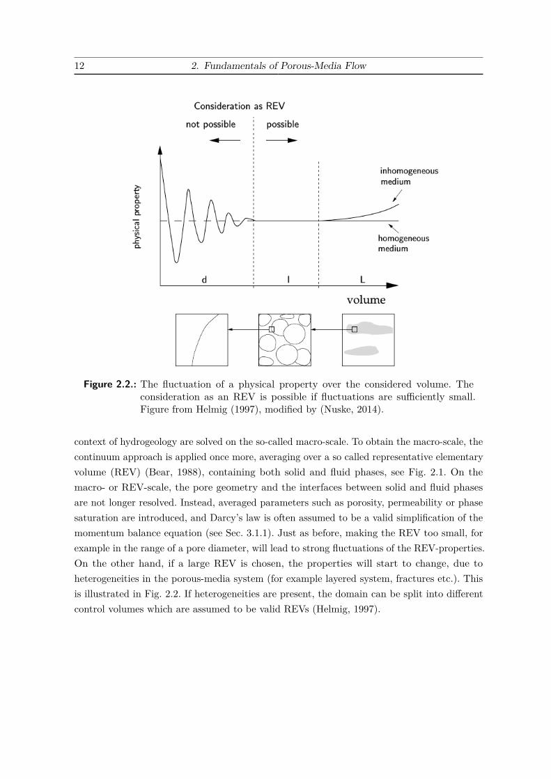
12 2. Fundamentals of Porous-Media Flow
Figure 2.2.: The fluctuation of a physical property over the considered volume. Theconsideration as an REV is possible if fluctuations are sufficiently small.Figure from Helmig (1997), modified by (Nuske, 2014).
context of hydrogeology are solved on the so-called macro-scale. To obtain the macro-scale, thecontinuum approach is applied once more, averaging over a so called representative elementaryvolume (REV) (Bear, 1988), containing both solid and fluid phases, see Fig. 2.1. On themacro- or REV-scale, the pore geometry and the interfaces between solid and fluid phasesare not longer resolved. Instead, averaged parameters such as porosity, permeability or phasesaturation are introduced, and Darcy’s law is often assumed to be a valid simplification of themomentum balance equation (see Sec. 3.1.1). Just as before, making the REV too small, forexample in the range of a pore diameter, will lead to strong fluctuations of the REV-properties.On the other hand, if a large REV is chosen, the properties will start to change, due toheterogeneities in the porous-media system (for example layered system, fractures etc.). Thisis illustrated in Fig. 2.2. If heterogeneities are present, the domain can be split into differentcontrol volumes which are assumed to be valid REVs (Helmig, 1997).

2.2. Local Thermodynamic Equilibrium 13
2.2. Local Thermodynamic Equilibrium
As a result of averaging over the micro-scale, parameters like pressure, temperature, andconcentration also have to be transferred to the macro-scale in order to describe flow andtransport processes in porous media. The simplest and most common assumption here is toassume local thermodynamic equilibrium. Local thermodynamic equilibrium states that withinan REV the following equilibria exist (Helmig, 1997):
• Mechanical Equilibrium: An equilibrium of forces is required, i.e. no resulting netforce. For an REV this means that on the interface between two phases the consideredforces should add up to zero. For a system with two fluid phases, the force balancecontains the fluid phase pressures of the wetting (pw), and non-wetting (pn) phase, aswell as the capillary pressure (pc): pn = pw + pc.
• Thermal Equilibrium: All temperatures of the different fluid (Tα), and solid phases(Ts) are the same, i.e. Ts = Tα = T .
• Chemical Equilibrium: All components’ rates of production are equal to their rates ofdestruction. For the distribution of a component between two phases n and w this impliesthat the fugacity of the component κ in each phase must be the same, i.e. fκn = fκw.
Using these assumptions greatly simplifies the solution of the resulting equations. If one wereto include local non-equilibrium processes, this would require knowledge of the interfacialareas between the phases (i.e. information available only on the micro-scale). This is discussedin detail in Nuske (2014) and will not be treated further here.
2.3. Properties of the Porous Medium
2.3.1. Porosity and Compressibility of the Porous Medium
The most important characteristic of a porous medium on the macro-scale is the ratio of thevolume of void space to the total volume. The resulting parameter is called porosity:
φ = VporeVtotal
. (2.1)
Considering only the void space that is accessible for flow leads to the definition of theso-called effective porosity. The effective porosity only considers the interconnected poreswithin Vpore (Bear, 1988). In this work, the porosity φ used is considered to be the effectiveporosity. In hydrogeology there are more definitions of porosity, such as the drainable porosity

14 2. Fundamentals of Porous-Media Flow
or specific yield. In these definitions Vpore is the volume of water which can be drained due togravitational forces, where a residual saturation Srw of water is left behind. This value has tobe equal to or smaller than the effective porosity. Defining φtotal with Vpore being the totalvoid volume (interconnected and disconnected pores) the drainable porosity can be defined as(Bear, 1988):
φdp = φtotal(1− Srw). (2.2)
A change in pressure may cause the bulk volume of a porous medium to change. The change canbe attributed to the compressibility of the solid grains and the so-called pore compressibility(consolidation of the void space). Usually the compressibility of the solid grains is consideredmuch smaller than the changes in porosity due to consolidation for hydrogeological problems(Bear, 1988). Hence, only the latter is considered here. The compressibility of the porousmedium can be defined similar to the compressibility of a fluid:
Cs = 1φ
dφ
dp. (2.3)
Under the assumption that the compressibility Cs itself is not a function of pressure, thefollowing dependence of porosity on pressure can be obtained after integration:
φ(p) = φinieCs(p−pini), (2.4)
where φini and pini are the initial porosity and pressure. Using the Taylor series approximationto express the exponential function leads to the function used in this work:
φ(p) = φini
(1 +X + X2
2
)with X = Cs(p− pini). (2.5)
This is the same function used in Schäfer et al. (2011) for the determination of far-field pressureduring long-term CO2 storage.
2.3.2. Permeability
Flow in a porous medium at small Reynolds numbers encounters a resistive force both fromthe fluid and the porous medium itself. This resistive force is proportional to the specificvolumetric flux. The reciprocal or inverse of the resistance caused by the porous medium iscalled permeability K. The permeability K is generally a tensor, as in most hydrogeologicalsystems, which are often layered systems, the permeability in the lateral direction of aformation is usually much higher than the permeability in the vertical direction. This is knownas anisotropy. If the permeability tensor is aligned with the coordinate axis of the system it has
2.4. Brine and CO2 15
a diagonal form. If isotropic conditions can be assumed, the permeability tensor reduces to ascalar value denoted here as k. If the permeability tensor varies with space, the porous mediumis heterogeneous. The permeability can be obtained directly from small scale (lab experiments)or large scale (pumping test) measurements. The permeability can also be estimated fromsemi-empirical relations that relate porosity, and an effective grain size to the permeability(Bear, 1988).
2.4. Brine and CO2
Mass/mole fraction, density, and viscosity are parameters obtained through averaging over themolecular scale. These parameters are used on the micro- as well as on the macro-scale. In thiswork, the relevant fluids are brine and CO2. Generally, the term brine is used for saltwaterwith a salinity above 5%. However, in this work the term brine or brine phase is also used forwater with low salinities. For CO2 injection, supercritical conditions are preferred, as CO2
exhibits liquid- and gas-like properties. Under supercritical conditions, the density of CO2 isgreater than the density in the gaseous state, which decreases the buoyant drive, and increasesstorage safety. On the other hand, the viscosity is smaller than in the liquid state, whichreduces the resistance during injection.
2.4.1. Components and Phases
A component is a chemically-independent species of a system, which means that its concentra-tion cannot be determined from the presence of other independent components in the system.In this work, water (H2O), carbon dioxide (CO2), and salt (NaCl) are considered independentcomponents.On the micro-scale every point in space is occupied by a certain phase, either fluid or solid(see Fig. 2.1 left). Phases can be composed of a single component or several components. Fluidphases can be liquid or gaseous. Liquid phases always form a sharp interface with other phases,if they are not completely miscible. A gaseous phase on the other hand, does not form a sharpinterface with other gaseous phases. The phases considered in this work are the liquid brinephase consisting of the components water and salt and the gaseous CO2 phase, consisting onlyof the component CO2.

16 2. Fundamentals of Porous-Media Flow
2.4.2. Mole and Mass Fractions
The mole fraction xκα is defined as the ratio of the number of molecules of a component κto the total number of molecules within a phase α. A mole fraction can be converted to amass fraction (ratio of the mass of a component κ to the total mass of a phase) through thefollowing relation:
Xκα = xκα
Mκ
Mα, (2.6)
where Mα is the average molar mass of a phase. It is the weighted arithmetic mean of themolar masses Mκ of the components weighted by the mole fractions xκα:
Mα =∑κ
Mκxκα. (2.7)
Given n− 1 mole or mass fractions of a phase comprising n components the composition ofthe phase is defined, as the sum of the mole and mass fractions has to be one:
∑κ
xκα =1 and (2.8)∑κ
Xκα =1. (2.9)
In this work, the term salinity is synonymous to the salt mass fractionXSw, where the component
index S stands for salt, and the phase index w for the wetting phase brine.
2.4.3. Density
The density of a phase %α can be defined as its mass per volume. It can also be expressed interms of moles per volume in which case it is denoted here as %mα . If the density in terms ofmass is known it can be converted to a molar density with the average molar mass:
%mα = %α
Mα. (2.10)
For the simulation of CO2 sequestration, the density of brine is often considered a functionof temperature, pressure, and the mass fractions of dissolved salt and CO2 (Darcis, 2012;Bielinski, 2006). Assuming chemical equilibrium for the mass transfer of CO2 and waterbetween the brine and CO2 phases, the mass fractions of CO2 in brine are in the order of 1to 6%, under relevant temperature and pressure conditions (see for example Darcis (2012)).Thus, the CO2 mass fraction increases the brine density. This is important to consider forlarge time scales, where the dissolution of CO2 is an important trapping mechanism, which

2.4. Brine and CO2 17
can be enhanced by convective mixing, due to density differences in the brine phase (seeSec. 2.7). However, for the applications presented in this work, where either short time scalesare considered or the fate of the injected CO2 is not the primary concern, the dissolution ofCO2 into the brine phase is not relevant, and therefore neglected.The equation of state defined by Batzle and Wang (1992) is used for calculating the brinedensity. The brine density is shown in Fix. 2.3 (left). Here the brine density is shown withrespect to temperature and salinity. The brine density decreases with increasing temperature.An increasing salinity has the opposite effect and increases the brine density. Although not
20 40 60 80 100
800
850
900
950
1000
1050
1100
1150
1200
1250
Density
Brine
[kg/m
3]
Temperature [◦C]
XSw = 0.0
XSw = 0.1
XSw = 0.2
XSw = 0.29
50 100 150 200 250 300
0
200
400
600
800
1000
1200
Density
CO
2[kg/m
3]
Pressure [bar]
30◦C45◦C60◦C75◦C
Figure 2.3.: The density of brine over temperature for different salinities (left) at a pressureof 100 bar. The density of CO2 over pressure for different temperatures (right).
shown here the relation is, to a lesser extent, also dependent on pressure, which is importantto consider, during the injection of CO2. For this case, the increasing pressure leads to anincrease of the brine density.
The CO2 density is calculated according to the relation defined by Span and Wagner (1996).Figure 2.3 (right) shows the CO2 density plotted over pressure for different temperatures. Thedensity of CO2 strongly increases close to the critical point (Tcrit = 31 ◦C, pcrit = 7.39 MPa).
2.4.4. Dynamic Viscosity
The dynamic viscosity µ is the proportionality factor relating shear stress to the velocitygradient. It can be expressed as follows:
τyx = µ∂vx∂y
, (2.11)

18 2. Fundamentals of Porous-Media Flow
where τyx is the shear stress in x-direction on a plane, whose outer normal is in y-direction,and ∂vx
∂y is the velocity gradient. The dynamic viscosity will simply be referred to as viscosityfrom now on. For a Newtonian fluid the viscosity is not a function of the velocity gradient.Considering laminar flow in a tube, a linear relationship between the average velocity andthe viscous force can be established. Similarly, for a porous medium on the macro-scale theviscous force is expressed as the resistance times the specific volumetric flux v:
Viscous Force = µK−1v, (2.12)
where the previously introduced permeability K depends on the porous medium and theviscosity depends on the fluid. For brine the viscosity is again calculated according to arelationship defined by Batzle and Wang (1992). Within this relationship the viscosity isconsidered to be a function of temperature and the salinity. The influence of pressure isneglected. The brine viscosity is shown in Fig. 2.4 (left). It is plotted over temperaturefor various salinities. The brine viscosity increases with increasing salinity and decreasingtemperature. The viscosity of gases is lower than that of liquids. The viscosity of supercritical
20 40 60 80 100
0
0.5
1
1.5
2
2.5
3
Viscosity
Brine
[10−
3Pas]
Temperature [◦C]
XSw = 0.0
XSw = 0.1
XSw = 0.2
XSw = 0.29
50 100 150 200 250 300
0
0.02
0.04
0.06
0.08
0.1
0.12
Viscosity
CO
2[10−
3Pas]
Pressure [bar]
30◦C45◦C60◦C75◦C
Figure 2.4.: The viscosity of brine over temperature for different salinities (left) at a pres-sure of 100 bar. The viscosity of CO2 over pressure for different temperatures(right).
CO2 is lower than the brine viscosity by roughly one order of magnitude. For CO2 viscositycalculations, the relationship by Fenghour et al. (1998) is used. The CO2 viscosity is plottedin Fig. 2.4 (right). A sharp increase of the CO2 viscosity is observed close to the critical point.Temperature and pressure both have opposing effects on the CO2 viscosity, similar to theCO2 density. Therefore, both viscosity and density, above supercritical conditions, are almostconstant over depth in hydrogeological systems, where temperature and pressure increase.

2.5. Multi-Phase Flow 19
2.5. Multi-Phase Flow
2.5.1. Saturation
The pore space is filled with fluid of one or more phases. The phases can be liquid or gaseous,in this case liquid brine and supercritical CO2. On the macro-scale, the amount of pore spaceoccupied by a phase within an REV is called saturation Sα where α denotes the phase index:
Sα = VαVpore
with 0 ≤ Sα ≤ 1. (2.13)
The sum of the saturations over all fluid phases present within an REV must be 1:
∑α
Sα = 1. (2.14)
If one phase is replaced by another phase, usually some amount of the displaced phase staysin the REV. This amount is referred to as the residual saturation Srα.
2.5.2. Capillary Pressure
The capillary pressure is defined as the pressure difference between two phases on the fluid-fluidinterface:
pc = pn − pw. (2.15)
On the micro-scale, where the position of fluid-fluid and fluid-solid interfaces is known, adriving force evolves due to one phase’s higher affinity to connect with the solid phase. Thephase with the higher affinity is called the wetting phase. Considering a circular tube withwater as the wetting phase (w) and air as the non-wetting phase (n), the wetting phase mayrise against the gravitational force. On the micro-scale this driving force, i.e. the capillarypressure can be expressed by the Young-Laplace equation:
pc = 2σcosαr
, (2.16)
where σ is the surface tension between the two fluid phases, α is the contact angle betweenthe wetting phase and the solid phase and r is the radius of the tube. With this equation itbecomes clear that a decrease of the radius of the tube will lead to an increase in capillarypressure. To transfer the concept of capillary pressure to the macro-scale it is necessary toestablish a relationship between capillary pressure and the previously introduced saturation.
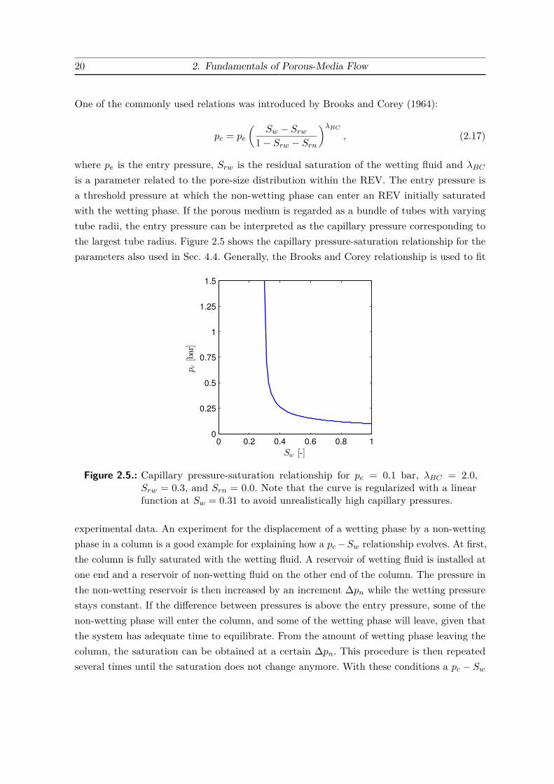
20 2. Fundamentals of Porous-Media Flow
One of the commonly used relations was introduced by Brooks and Corey (1964):
pc = pe
(Sw − Srw
1− Srw − Srn
)λBC, (2.17)
where pe is the entry pressure, Srw is the residual saturation of the wetting fluid and λBCis a parameter related to the pore-size distribution within the REV. The entry pressure isa threshold pressure at which the non-wetting phase can enter an REV initially saturatedwith the wetting phase. If the porous medium is regarded as a bundle of tubes with varyingtube radii, the entry pressure can be interpreted as the capillary pressure corresponding tothe largest tube radius. Figure 2.5 shows the capillary pressure-saturation relationship for theparameters also used in Sec. 4.4. Generally, the Brooks and Corey relationship is used to fit
0 0.2 0.4 0.6 0.8 10
0.25
0.5
0.75
1
1.25
1.5
pc[bar]
Sw [-]
Figure 2.5.: Capillary pressure-saturation relationship for pe = 0.1 bar, λBC = 2.0,Srw = 0.3, and Srn = 0.0. Note that the curve is regularized with a linearfunction at Sw = 0.31 to avoid unrealistically high capillary pressures.
experimental data. An experiment for the displacement of a wetting phase by a non-wettingphase in a column is a good example for explaining how a pc−Sw relationship evolves. At first,the column is fully saturated with the wetting fluid. A reservoir of wetting fluid is installed atone end and a reservoir of non-wetting fluid on the other end of the column. The pressure inthe non-wetting reservoir is then increased by an increment ∆pn while the wetting pressurestays constant. If the difference between pressures is above the entry pressure, some of thenon-wetting phase will enter the column, and some of the wetting phase will leave, given thatthe system has adequate time to equilibrate. From the amount of wetting phase leaving thecolumn, the saturation can be obtained at a certain ∆pn. This procedure is then repeatedseveral times until the saturation does not change anymore. With these conditions a pc − Sw
2.5. Multi-Phase Flow 21
relationship can be obtained, as shown in Fig. 2.5. The left over wetting phase within thecolumn corresponds to the residual water saturation Srw. If the obtained pc−Sw relationship isused as a constitutive relationship for a simulation an assumption of local capillary equilibriumor local mechanical equilibrium at all times is implicitly made. The process of the wettingphase being displaced by the non-wetting phase is called drainage. Wetting phase displacingthe non-wetting phase is called imbibition. It has to be mentioned that the pc−Sw relationshipis not a unique relationship. Depending on the direction of the process (imbibition or drainage)different curves will be obtained (hysteresis). Hysteresis can be important if imbibition ordrainage both occur sequentially during a process for example:
• During CO2 injection, drainage occurs. After the injection, brine will flow back towardsthe well (imbibition).
• Sub-surface methane storage requires injection and extraction of methane depending onsupply and demand. Here drainage and imbibition follow sequentially.
For the applications considered in this work only, drainage is of importance, hence hysteresisis not considered. More information on the implementation of models accounting for hysteresiscan be found for example in Papafotiou (2008).
2.5.3. Relative Permeability
When two or more phases are present in the pore space, the resistance to flow will increasecompared to similar systems with only one phase. On the macro-scale, this additional resistanceis integrated into the viscous force using the term relative permeability krα. The relativepermeability is a function of the phase saturation:
0 ≤∑α
krα(Sα) ≤ 1. (2.18)
On the micro-scale there are several effects that contribute to this resistance (Helmig, 1997):
• Simplifying the porous medium to a bundle of tubes, the relative permeability isproportional to the cross-sectional area available for each phase.
• Extending this analogy to a system of tubes of variable radius, either filled with wettingor non-wetting phase, the tubes with small radii are occupied by the wetting phase.Resistance against wetting phase flow is therefore increased by higher viscous forces, which

22 2. Fundamentals of Porous-Media Flow
can be expressed as a function of the square of the tube radius after Hagen-Poiseuille(neglecting the gravitational force):
8µwr2 vw = −∂pw
∂x. (2.19)
• Additionally, as the larger pores are occupied by the non-wetting phase the wettingphase has to flow around these large pores through smaller pores. This increases theflow path and therefore the tortuosity.
All the above micro-scale effects are represented on the macro-scale by the single parameter:relative permeability. In the general case, the relative permeability is an anisotropic tensorialquantity. Similar to the intrinsic permeability tensor, the relative permeability may changewith direction, due to a heterogeneous distribution of the fluid phases. This leads to preferentialflow paths. However, in most practical applications, the relative permeability of a phase isassumed to be a scalar related to the phase’s saturation, as data for justifying a more complexdescription is usually not available. However, upscaling relative permeabilities from a highlyresolved geological description to a coarse geological description, may also require the use oftensorial relative permeabilities, see for example Wolff (2013). There exist different krα − Sαrelationships, one of the most commonly used is the relationship by Brooks and Corey (1964):
krw = (Se)2+3λBCλBC ,
krn =(1− Se)2 (1− Se)2+λBCλBC ,
with Se = Sw − Srw1− Srw − Srn
.
(2.20)
The relationship is shown in Fig. 2.6 for the parameters used in Sec. 4.4. It can be seen thatthe relative permeability of each phase becomes zero, as the phase’s residual saturation isapproached. Further, krw shows a small slope for low values of Sw which can be attributed tothe wetting phase occupying small pores at low saturation which contribute little to flow. Byassuming that the non-wetting phase occupies the larger pores, and that the wetting phaseoccupies the smaller pores capillary equilibrium is implicitly assumed within an REV. Thekrα − Sw relationship is hysteretic in nature, just as the pc − Sw relationship is.

2.6. Transport Processes 23
0 0.2 0.4 0.6 0.8 10
0.2
0.4
0.6
0.8
1
kr[-]
Sw [-]
krwkrn
Figure 2.6.: Relative permeability-saturation relationship for λBC = 2.0, Srw = 0.3, andSrn = 0.0.
2.6. Transport Processes
In this section, the basic transport processes and their relevance for the further applicationsare presented.
2.6.1. Advection
If a fluid moves the components present in the fluid will also move with the fluid. This transportmechanism is known as advective transport or advective flow and can be expressed per unitarea of a porous medium as:
Jaκ = φXκ%va, (2.21)
where Xκ is the mass fraction of a component, % the density and va is an average velocity ofthe fluid (per unit area of the fluid phase). This definition is also valid for multi-phase flow,where the components of a phase are being transported with a specific phase flux vα. In thecontext of CO2 sequestration, the term advection is often used to describe the flow resultingfrom the injection of CO2, whereas the term buoyancy is used to describe gravity-inducedflow, although this flow is strictly speaking also a form of advective flow.

24 2. Fundamentals of Porous-Media Flow
2.6.2. Diffusion
Diffusion is a mass transport process which is caused by the Brownian motion of molecules.Considering a fluid with a dissolved component κ on the micro-scale the binary diffusive fluxmay be expressed in terms of a mole fraction gradient (Taylor and Krishna, 1995):
jκdiff = −%mDκm gradxκ, (2.22)
where %m is the molar density and Dm is the molecular Diffusion coefficient. Note that theindex of the solvent or fluid phase is omitted in this section. Equation 2.22 is known as Fick’slaw. Another common way to express Fick’s law is to use the mass fraction gradient instead ofa mole fraction gradient (Taylor and Krishna, 1995; Diersch and Kolditz, 2002; Bear, 2005).On the macro-scale, a diffusive flux per unit volume of the porous medium can be obtained byaveraging Eq. 2.22 (Bear, 2005):
Jκdiff = jκdiff = −φ%mT(φ)Dκm gradxκ, (2.23)
where T(φ) is the tortuosity tensor, defined by a function of the porosity φ. In this work, anisotropic medium is assumed and the tortuosity is simplified to φ. Finally, the macro-scalediffusion coefficient of the porous medium is defined as:
Dκpm = φ2Dκ
m. (2.24)
2.6.3. Mechanical Dispersion
Mechanical dispersion leads to the spreading of a dissolved component within a moving fluid ina porous medium. The term mechanical indicates that dispersion (spreading) only takes placeif the fluid is moving with an average velocity va (per unit area of the fluid phase). On themicro-scale the evolving velocity distribution of a fluid in a pore (parabolic in case of laminarflow) will lead to varying velocities in magnitude over the cross-section of the pore. Moleculardiffusion will act mainly in the direction normal to the streamlines in order to equilibratethe arising concentration gradients. Additionally, the structure of the interconnected porespace will lead to deviations from the mean direction of flow. Both these effects lead to anincreased spreading. When averaging over an REV, these effects lead to an additional so-calleddispersive flux. Bear (2005) introduces another scale, larger than the macro-scale, to arrive ata new continuum, referred to as megascopic-scale. On this scale, the effects of macro-scaleheterogeneities are described through macro dispersion. The formulation of dispersion onthe megascopic-scale can be defined in the same way as for the macro-scale. The following

2.7. Variable-Density Flow 25
formulation of dispersive flux per unit area of porous medium is often used independent of thescale:
Jκdisp = −φ%mDdisp gradxκ, (2.25)
where Ddisp is the hydrodynamic dispersion tensor. It can be formulated depending on thedirection of the average fluid velocity va:
Ddisp = va ⊗ va|va|
(αl − αt) + I (φDκm + αt|va|) , (2.26)
where αl and αt are the longitudinal and transversal dispersivities, respectively. αl is a measurefor the scale of the heterogeneities of the problem. According to Bear (2005) the choice ofthis parameter thus depends on the scale of the problem, as the dimension ot the “sub-scale“heterogeneities, i.e. the heterogeneities not resolved, will increase if the scale of the problemincreases. He states further that αl = L/10, where L is the size of the domain of interest, canbe a first guess. Similarly, he roughly approximates αt to be αl/10. Notice that in Eq. 2.26the diffusive flux is already included.
2.7. Variable-Density Flow
In many applications, the density of a fluid phase cannot be considered uniform, within thedomain of interest. This variability in density needs to be considered in the gravity or buoyancyterm of the momentum balance. A system of equations describing single-phase, variable-densityflow is generally fully coupled and non-linear, as the density and the viscosity are functions oftemperature, salinity, and pressure. For example, the density of brine is mainly a function oftemperature and salinity (see Fig. 2.3). This has the consequence that the bulk brine flow,depending on the brine density, cannot be treated independently from the transport of salt orheat.
Variable-density flow can be stable or unstable. Unstable situations arise if heavy fluid issituated above lighter fluid. In the context of CO2 sequestration such situations may occurif brine, fully saturated with CO2 at the CO2 plume, is situated above lighter brine withoutdissolved CO2, see for example Gläser (2011). If no other external forces act, which is the caseafter the injection is over, free convection may occur, where the fluid flow is driven entirely bydensity differences. However, if dispersive flow is large compared to the density-driven flow, thefront can stabilize. The dimensionless Rayleigh Number describes the ratio of density-drivenflow and dispersive flow. The Rayleigh number is used as a measure of stability (Diersch and

26 2. Fundamentals of Porous-Media Flow
Kolditz, 2002):Ra = dk∆%g
µD, (2.27)
where d is a characteristic system height. In a homogeneous horizontally aligned aquifer, anatural choice for d would be the aquifer thickness. D stands for the magnitude of dispersivefluxes arising either from thermal diffusivity or hydrodynamic dispersion of a dissolvedcomponent
(||Ddisp||
). The remaining term
(k∆%gµ
)can be interpreted as gravitationally
induced flux, due to density differences.
In this work, stable conditions are assumed, where the brine density increases with depth, dueto an increase of salinity. In the model presented in Chapter 5, a stable layering is combinedwith advective flow, caused by groundwater recharge and the injection of super-critical CO2.A similar situation is considered in the experiments conducted by Oswald and Kinzelbach(2004). They set up experiments, better known as the saltpool benchmark, whose results arewidely used to validate numerical models (Bastian et al., 2001; Diersch and Kolditz, 2002;Johannsen et al., 2002). These experiments deal with upconing as a result of water extractionin an initially stably layered system, with freshwater on top and salt water below. The salinityof the bottom layer is varied. The higher the salinity in the bottom layer, the higher thenon-linearities, and the more challenging the problem becomes for the numerical simulator.Results of this benchmark will be shown in Sec. 5.4.2. Besides the brine density, the viscosityof brine is also a function of salinity and the temperature, and therefore affects the flow field.Magri et al. (2009a) who consider a comparable hydrogeological system as in Chapter 5, statethat the effect of a variable viscosity has a significant impact on the overall flow field.
3. Model Concepts
In this chapter, the balance equations and solution methods that are applied in Chapters 4and 5 will be presented. To start, all relevant balance equations will be briefly introducedwithout thorough derivation (Sec. 3.1). Following this, analytical and numerical solutionmethods are explained in Sec. 3.2 and 3.3.
3.1. Balance Equations
The mass balance equations for a single-phase two-component model (1p2c), a two-phase model(2p) without component transport, and two-phase three-component model (2p3c) are shownin this section, along with the generalization of Darcy’s law. Additionally, the fractional-flowformulation, and the sharp-interface formulation are derived from the 2p balance equations.
3.1.1. Momentum Balance Equation
The hydrogeological systems under consideration in this work are described as a porous-mediasystem, assuming laminar flow throughout. The inertial force (convective and local) is assumedto be much smaller than the viscous force. Additionally, the viscous force (i.e. the resistiveforce opposite to the flow direction) is proportional to the specific volumetric flux. This typeof flow is also known as creeping flow (Bear, 1988). The resulting momentum balance, alsocalled Darcy’s law, allows the explicit solution of the specific volumetric flux vf (per unit areaof the porous medium):
vf = −Kµ
( grad p− %g) . (3.1)
vf is also referred to as the filter or the Darcy velocity. If % and µ are assumed constant therelationship between the specific volumetric flux and the pressure gradient is linear, just asin a potential flow. This is advantageous, as the solution of a complex flow problem can beachieved by superimposing the solutions of simpler subproblems. Darcy’s law was originallyderived from 1D column experiments, thus Eq. 3.1 is a generalization of Darcy’s law, which isapplicable to 3D flow in anisotropic media in terms of pressure instead of hydraulic head (Bear,
28 3. Model Concepts
1988). Whether Darcy’s law is a valid assumption or not can be tested with the dimensionlessReynolds number, a ratio of inertial and viscous forces:
Re = %d|vf |µ
. (3.2)
Here, d is defined as a characteristic grain diameter such as for example d10, (i.e. the grain sizeexceeding 10% of the other diameters by weight). Bear (1988) concludes that an effective upperlimit of validity of Darcy’s law, for the cases reported in literature, would be a Reynolds numberbetween 1 and 10. It is assumed that this condition is fulfilled in this work. For convenience,the specific volumetric flux vf will be referred to as v from now on. Equation 3.1 can befurther extended to account for the flow of multiple mobile phases in the pore space (Helmig,1997):
vα = −krαKµα
( grad pα − %αg) . (3.3)
Here, every phase has its own specific volumetric flux vα and the additional resistance causedby multiple phases present in the pore space is accounted for by the term relative permeabilitykrα, previously introduced in Sec. 2.5.3.
3.1.2. Mass Balance Equations
The following section will present the different mass balance equations that will be used inthis work. The generalization of Darcy’s law, described in the last section, is directly insertedinto all mass balance equations.
One-Phase Two-Component Formulation (1p2c)
First the mole balance or continuity equation for a single phase without additional componentsis formulated:
∂(φ%mw )∂t
= div{−%mw
Kµw
( grad pw − %wg)}
+ qw. (3.4)
The mole balance equation is written in terms of the brine phase (index w). %m is a molardensity whereas % denotes the mass density. In the storage term, the porosity φ as a functionof pressure, is considered using Eq. 2.5. Further, the density of brine in the storage term is afunction of pressure, temperature, and salinity, see Sec. 2.4.3. qw represents a molar source orsink term for the brine phase.
3.1. Balance Equations 29
Using Eq. 3.4 as a total mole balance, another equation is needed to describe the transport ofthe component salt:
∂(φ%mw xSw)∂t
= div{−%mw xSw
Kµw
( grad pw − %wg)− φ%mwDdisp gradxSw}
+ qS . (3.5)
Here, xSw is the mole fraction of salt in the brine phase. The equation considers the advectivetransport of salt and includes a term accounting for dispersive fluxes, as discussed in Sec. 2.6.3.Equations 3.4 and 3.5 together form the 1p2c balance equations. Another equation is requiredto close the system (previously discussed in Sec. 2.4.2):
∑κ
xκα = 1. (3.6)
This equation relates the mole fractions within a phase and is valid for all compositionalmodels.
Two-Phase Formulation (2p)
The mass balance equations for two-phase immiscible flow are formulated as follows:
φ∂(%αSα)
∂t= div
{−%α
krαµα
K( grad pα − %αg)}
+ qα (3.7)
α ∈ {w, n}.
They consist of two mass balance equations: one for the wetting phase brine (w) and one forthe non-wetting phase CO2 (n). The multi-phase flow extension of Darcy’s law (Eq. 3.3) isused. Near the injection well, the total compressibility is dominated by the compressibilityof CO2. The 2p model will be used to describe the propagation of the CO2 front near theinjection well. Far-field pressure buildup is therefore less relevant (Chapter 4). Thus, the 2pmodel does not consider the compressibility of the porous medium, meaning that φ is notincluded in the time derivative of the storage term. qα is a source or sink term for phase α.Here, two additional closing relations are required for relating wetting and non-wetting phasepressures through the capillary pressure:
pn = pw + pc, (3.8)
and for relating the wetting and non-wetting phase saturation:
∑α
Sα = 1. (3.9)

30 3. Model Concepts
Two-Phase Fractional-Flow Formulation
The two-phase balance equations can be reformulated into a pressure and a saturation transportequation. For a more thorough derivation, see Helmig (1997).Assuming incompressibility, which requires the division of Eq. 3.7 by the phase density %αand the summation of the wetting and non-wetting mass balances, the following equation isobtained:
divvw + divvn + qw + qn = 0. (3.10)
Now a total phase flux vt can be introduced. This is the sum of the fractional fluxes, i.e. theindividual phase velocities:
vt = vw + vn. (3.11)
Hence, Eq. 3.10 becomes:divvt + qt = 0, (3.12)
where qt is the sum of the wetting and non-wetting source terms. This equation is knownas the pressure equation. The next step is to insert both phase velocities from Eq. 3.3 intoEq. 3.11. Using the closing relation pn = pw + pc, one of the pressures can be replaced. In thiscase, pn is replaced:
vt = −K (λw + λn) grad pw + λn grad pc − (λw%w + λn%n) g. (3.13)
To simplify the notation, phase mobilities, λw = krwµw
and λn = krnµn
, are introduced. Further,the total mobility λt = λw + λn and the fractional flow function fα = λα
λtare defined. After
several reformulation steps, the following relation for vt can be obtained:
vt = −λtK(
grad pw + fn grad pc − (fw%w + fn%n) g). (3.14)
In order to obtain the saturation equations, the phase velocities vα have to be expressed interms of the total velocity. To solve the system of equations with two unknowns (one phasepressure and one phase saturation) only one saturation equation is required together withthe pressure equation. Here, the saturation equation for the wetting phase is derived. SolvingEq. 3.3 for K grad pw and inserting this into Eq. 3.14 yields:
vw = fwvt − λnfwK grad pc − λnfw (%w − %n) Kg. (3.15)

3.1. Balance Equations 31
Inserting Eq. 3.15 into Eq. 3.7 and again assuming incompressibility results in the saturationequation:
φ∂Sw∂t
= div{fwvt − λnfwK grad pc − λnfw (%w − %n) Kg
}+ qw. (3.16)
Equations 3.12 and 3.16 make up the fractional-flow formulation. In order to better distinguishthe dominant driving forces, the dimensions are removed following the approach by Kopp et al.(2009a). At first, three independent characteristic values have to be defined:
• lcr = system length or width of a saturation front,
• vcr = characteristic Darcy velocity, and
• pcr = capillary-pressure drop over the system length or width of a saturation front.
Using these characteristic values, the following terms are non-dimensionalized:
div = div lcr, grad = grad lcr, t = tvcrφlcr
, pc = pcpcr
, vt = 1vcr
vt. (3.17)
Now the dimensions of the saturation equation (Eq. 3.16) are removed. Additionally, isotropicconditions are assumed and g is replaced by g grad z:
∂Sw
∂t= div
{fwvt −
λnfwkpcrvcrlcr
grad pc − λnfw (%w − %n) kg grad z}. (3.18)
Finally, the capillary (Ca) and gravitational numbers (Gr) along with another dimensionlessparameter C are introduced:
Ca = kpcrµnvcrlcr
, Gr = (%w − %n)gkµnvcr
, C = krnfw. (3.19)
Ca and Gr will be discussed further in Chapter 4. Inserting these dimensionless numbers intothe saturation equation yields:
∂Sw
∂t= div
{fwvt − CCa grad pc − CGr grad z
}. (3.20)
Note that Ca and Gr could also be defined with the brine viscosity term in the denominator,if C were defined as C = krwfn. Similar to the saturation equation, the pressure equation(Eq. 3.12) can also be non-dimensionalized using the above dimensionless numbers. Furtheranalysis on this topic can be found in Kopp et al. (2009a).

32 3. Model Concepts
Two-Phase Sharp-Interface Formulation
Another formulation of the two-phase flow balance equations (Eq. 3.7) exists when assumingvertical equilibrium. Vertical equilibrium is based on the Dupuit assumption, where verticalfluxes are neglected. The assumption is valid if the lateral extent of a formation is much largerthan its vertical extent. This is usually the case for saline aquifers, where CO2 can be stored.An exception is the area close to the injection well, where the values of the gravitational number(Gr) are very low and the viscous forces dominate. If solved numerically, the main advantage ofthe vertical-equilibrium assumption is that the system is reduced to two dimensions. However,for specific cases as presented below, the formulation can be further reduced from a systemof non-linear partial differential equations to a system of non-linear ordinary differentialequations. The approach presented in Nordbotten and Celia (2006) is used for the derivationof a sharp-interface model. As the aim is to show the main assumptions and explain theresulting equations, the derivation will not be in full detail. For a more thorough derivationsee Nordbotten and Celia (2006).
Due to the vertical-equilibrium assumption, the CO2 is assumed to immediately gather belowthe top of the injection layer with two domains forming: the brine domain, and the CO2
domain. Both domains are separated by a sharp interface. Such a system is shown in Fig. 3.1.The brine domain is fully saturated with brine, while the CO2 domain contains both the
Hh(r, t)z
r
Figure 3.1.: Injection of CO2 in a confined aquifer. The vertical pressure distribution isassumed hydrostatic for the sharp interface model.
CO2 and the residual brine, i.e. Sn = (1− Srw). As saturations within the two domains arefixed, the relative permeabilities (krα) are constant, considerably simplifying the problem. Forsimplifying Eq. 3.7 further, the following assumptions are made:
• a radially symmetric domain with an injection well at the center,
• the top and bottom of the injection formation are orthogonal to the gravity vector,
• the system is incompressible,
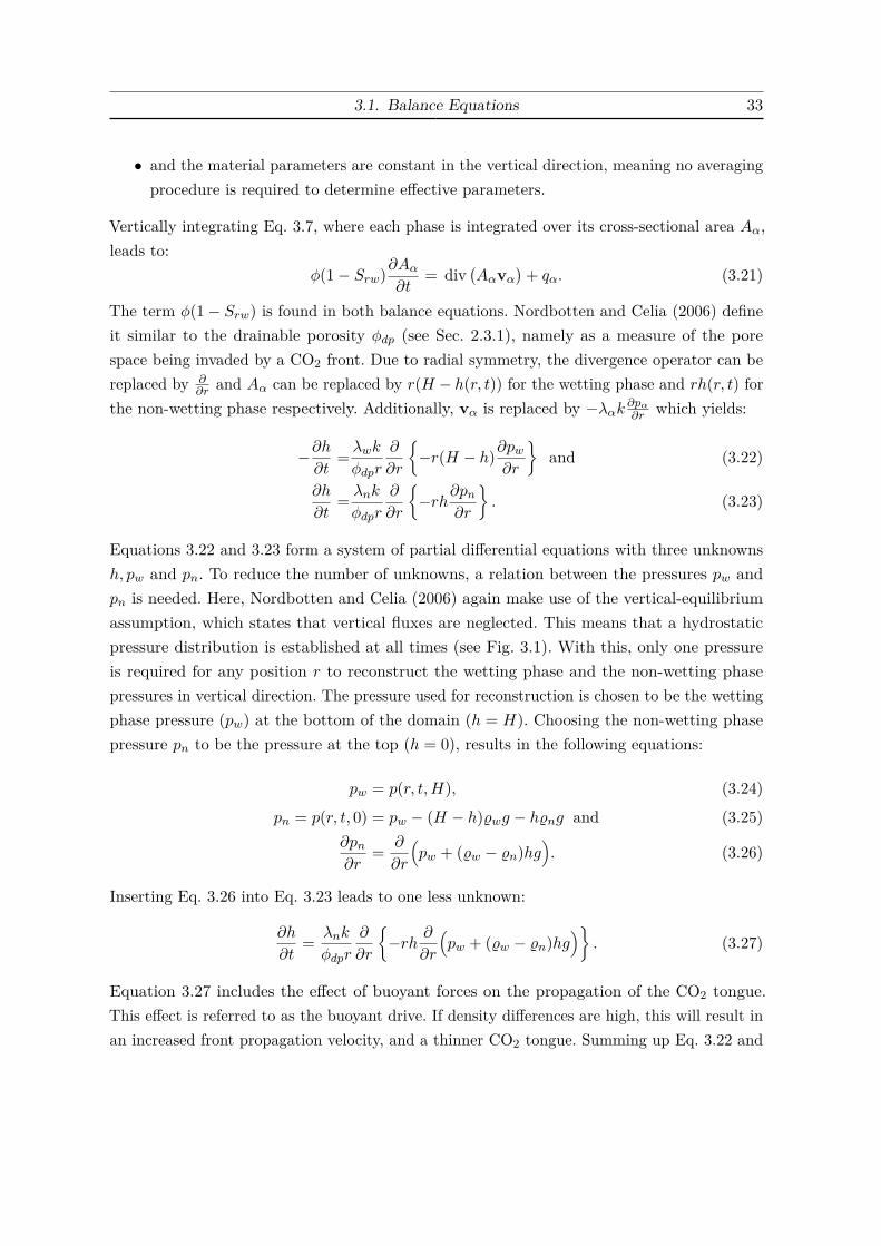
3.1. Balance Equations 33
• and the material parameters are constant in the vertical direction, meaning no averagingprocedure is required to determine effective parameters.
Vertically integrating Eq. 3.7, where each phase is integrated over its cross-sectional area Aα,leads to:
φ(1− Srw)∂Aα∂t
= div(Aαvα
)+ qα. (3.21)
The term φ(1− Srw) is found in both balance equations. Nordbotten and Celia (2006) defineit similar to the drainable porosity φdp (see Sec. 2.3.1), namely as a measure of the porespace being invaded by a CO2 front. Due to radial symmetry, the divergence operator can bereplaced by ∂
∂r and Aα can be replaced by r(H − h(r, t)) for the wetting phase and rh(r, t) forthe non-wetting phase respectively. Additionally, vα is replaced by −λαk ∂pα∂r which yields:
−∂h∂t
= λwk
φdpr
∂
∂r
{−r(H − h)∂pw
∂r
}and (3.22)
∂h
∂t= λnk
φdpr
∂
∂r
{−rh∂pn
∂r
}. (3.23)
Equations 3.22 and 3.23 form a system of partial differential equations with three unknownsh, pw and pn. To reduce the number of unknowns, a relation between the pressures pw andpn is needed. Here, Nordbotten and Celia (2006) again make use of the vertical-equilibriumassumption, which states that vertical fluxes are neglected. This means that a hydrostaticpressure distribution is established at all times (see Fig. 3.1). With this, only one pressureis required for any position r to reconstruct the wetting phase and the non-wetting phasepressures in vertical direction. The pressure used for reconstruction is chosen to be the wettingphase pressure (pw) at the bottom of the domain (h = H). Choosing the non-wetting phasepressure pn to be the pressure at the top (h = 0), results in the following equations:
pw = p(r, t,H), (3.24)
pn = p(r, t, 0) = pw − (H − h)%wg − h%ng and (3.25)∂pn∂r
= ∂
∂r
(pw + (%w − %n)hg
). (3.26)
Inserting Eq. 3.26 into Eq. 3.23 leads to one less unknown:
∂h
∂t= λnk
φdpr
∂
∂r
{−rh ∂
∂r
(pw + (%w − %n)hg
)}. (3.27)
Equation 3.27 includes the effect of buoyant forces on the propagation of the CO2 tongue.This effect is referred to as the buoyant drive. If density differences are high, this will result inan increased front propagation velocity, and a thinner CO2 tongue. Summing up Eq. 3.22 and

34 3. Model Concepts
3.27 and integrating the resulting equation from 0 to r yields:
const = kr
{(H − h)λw
∂pw∂r
+ hλn∂
∂r
(pw + (%w − %n)hg
)}. (3.28)
Here, the integration constant can be physically interpreted as a total flow in the radialdirection. The assumption of a constant injection rate Qwell leads to the integration constant−Qwell
2π . Inserting the integration constant, solving the equation for ∂pw∂r , and inserting it into
Eq. 3.22 leads to the following equation:
∂h
∂t= λwk∆%g
φdpr
∂
∂r
{r(H − h)hλn
(H − h)λw + hλn
∂h
∂r+ (H − h)Qwell
2πk((H − h)λw + hλn)1
∆%g
}, (3.29)
which is a non-linear partial differential equation with the unknown h. In their derivation of aself-similar solution for h(r, t), Nordbotten and Celia (2006) bring Eq. 3.29 into a dimensionlessform. Further, they introduce a scaling variable χ which they use in order to find a stationarysolution that satisfies a non-linear ordinary differential equation. The steps used to obtain thisequation are not shown here. The presentation is restricted to showing the resulting equation:
0 = χ−[1 + Γλχ∂(h′)2
∂χ
]2λ
(1 + (λ− 1)h′2)
+4Γλ 1− h′1 + (λ− 1)h′
[h′ + χ
∂h′
χ+ h′χ
∂2h′
∂χ2
(∂h′
∂χ
)−1].
(3.30)
Within this equation the following dimensionless variables are defined:
Γ = 2π∆%gkλwH2
Qwell, λ = λn
λw, h′ = h
H,
τ = Qwellt
2πHkφdp, η = r√
k, χ = η
τ,
(3.31)
where Γ is a different formulation of the gravitational number and χ is the remaining indepen-dent variable which is the ratio of dimensionless space and time. Equation 3.30 is valid for(∂h′
∂χ
)6= 0, which physically means that the CO2 tongue has to become thinner (monolithically)
for increasing χ. If Γ becomes small, for example due to a high injection rate, Eq. 3.30 can besolved explicitly for h′ with:
h′ =
1 for χ ≤ 2
λ ,
1λ−1
(√2λχ − 1
)for 2
λ < χ < 2λ,
0 for χ ≥ 2λ.
(3.32)
Here, the dimensionless height of the CO2 front depends solely on the viscosity ratio. For large
3.2. Analytical Methods 35
Γ, the ordinary differential equation (Eq. 3.30) has to be solved numerically. This requiresthat the following boundary conditions are fulfilled:
• an outer radius rmax where h = 0 exists,
• and the volume balance:∫ rmax
0φdph(r, t)2πrdr = Qwellt or
∫ χmax
0h′(χ)dχ = 2 (3.33)
is satisfied.
Equations 3.30 and 3.33 are a system of non-linear ordinary differential equations that haveto be solved for h′(χ) numerically.
Two-Phase Three-Component Formulation (2p3c)
The most complex model used in this work accounts for two-phase miscible flow and three-component transport. One mole balance equation for each of the three components is formu-lated:
∂(φ∑α %mα x
καSα)
∂t=∑
α
div{−%mα xκα
krαµα
K( grad pα − %αg)− %mαDκpm,α grad xκα
}+ qκ
α ∈ {w, n} and κ ∈ {H2O,CO2, S}.
(3.34)
In this system, the fluid phases are brine (w) and CO2 (n), and the components are water,CO2, and salt. However, for the application in mind, the dissolution of CO2 in brine andvice versa is neglected as the fate of the CO2 is not the primary interest. Similarly, the saltcomponent is only considered in the brine phase. As a result, the brine phase consists only ofwater and salt, and the CO2 phase only of CO2. The compressibility of the porous mediumas well as the two fluid phases are considered. The flux term considers advection as well asmolecular diffusion. Equations 3.6, 3.8 and 3.9 are required as closing relations.
3.2. Analytical Methods
In this section, analytical solutions for some of the formulations above are presented. Thesesolutions are applicable when the physics and the geometry of a problem are significantly

36 3. Model Concepts
simplified. On the one hand, they can be used for making fast predictions if the available datais not sufficient for more complex approaches, or if the computational demand is too high fornumerical models. On the other hand, analytical solutions can be used to verify numericalmodels, i.e. to see if the implementation of a numerical model is correct.
3.2.1. Analytical Solution for Estimating the Volumetric CO2 Storage Efficiency
Okwen et al. (2010) presented an analytical solution for calculating the volumetric storageefficiency of a radially symmetric reservoir with a vertical injection well, a constant injectionrate, homogeneous permeability and porosity, and constant fluid parameters. This methodwill be referred to here as the Okwen-Method. The Okwen-Method is based on the previouslyintroduced non-linear ODE (Eq. 3.30) derived by Nordbotten and Celia (2006). Therefore,the underlying assumption of a vertical equilibrium and a sharp interface between the CO2
and brine phase (i.e. no capillary fringe and no mass transfer between the two phases) is alsomade here. The aim of this method is to determine the volumetric storage efficiency, which isdefined as:
E = VinjectedVformation
= Qwellt
φdp2πH(rmax)2 . (3.35)
Here Vinjected is the injected volume of CO2 and Vformation is the available pore space in thereservoir. Okwen et al. (2010), like Nordbotten and Celia (2006), show that for small gravi-tational numbers the volumetric storage efficiency becomes independent of the gravitationalnumber and depends only on the mobility ratio (λ) and the residual saturation of brine (Srw).They use the definition of the gravitational number Γ shown in Eq. 3.31, defined by Nordbottenand Celia (2006), which includes the mobility of brine instead of CO2. Inserting the definitionsof dimensionless space (η) and time (τ) given in Eq. 3.31 into Eq. 3.35 yields:
E = (1− Srw)τmaxη2max
= (1− Srw)χmax
. (3.36)
As mentioned previously, χmax can be calculated explicitly with Eq. 3.32 if Γ is sufficientlysmall. If gravitational forces cannot be neglected, Eq. 3.30 has to be solved numericallytogether with Eq. 3.33. To avoid this, the Okwen-Method uses a polynomial function with Γand λ as independent variables to explicitly calculate the volumetric storage efficiency whengravitational forces are not negligible. For this, they solved the non-linear ordinary differentialequation (Eq. 3.30) to obtain χmax for different values of Γ (0.5 ≤ Γ ≤ 50) and λ (5 ≤ λ ≤ 20)and fitted the results with a polynomial.
3.2. Analytical Methods 37
The resulting equation for estimating storage efficiency E according to the Okwen-Method is:
E = (1− Srw) 1λ
0 ≤ Γ < 0.5,
E = 2(1− Srw)(0.0324λ− 0.0952)Γ + (0.1778λ+ 5.9682)Γ1/2 + 1.6962λ− 3.0472
, (3.37)
0.5 ≤ Γ ≤ 50.
Storage efficiency in terms of mass per volume can easily be obtained by multiplying E withthe density of CO2 under reservoir conditions.
3.2.2. Single-Phase Injection in a Multi-Layer System with a Fault Zone
In this section, an analytical solution for determining leakage, due to brine injection in amulti-layer aquifer system, whose layers are connected by a fault zone, is presented. Theanalytical solution is based on the solution presented by Shan et al. (1995) for a two layersystem, and was extended by Zeidouni (2012) to account for the following conditions:
• a pressure jump across the fault plane,
• the inclusion of multiple aquifers above the injection layer.
The analytical solution will be referred to here as the Zeidouni-Method.
The set of governing equations is a simplification of Eq. 3.4. It is derived by assuming a constantbrine density and viscosity, a constant aquifer thickness, and a homogeneous permeabilityand porosity in each aquifer. Vertical fluxes in the aquifers are neglected based on the Dupuitassumption, except for the fault zone where vertical leakage may occur. The fault zone itselfis assumed to have no storage, and is aligned with the y-axis. The injection layer and eachoverlying aquifer is split into two regions for each side of the fault plane, see Fig. 3.2. Thegoverning equations for the injection layer and the overlying aquifers are denoted by thefirst index j for the aquifer number, with j = 1 for the injection layer, and the second index
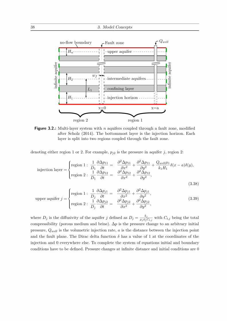
38 3. Model Concepts
infin
iteaq
uifer
x=0 x=a
intermediate aquifers
injection horizon
confining layer
upper aquifer
infin
iteaq
uifer
QwellFault zone
H1
H2
Hn
L1
wf
region 2 region 1
no-flow boundary
Figure 3.2.: Multi-layer system with n aquifers coupled through a fault zone, modifiedafter Scholz (2014). The bottommost layer is the injection horizon. Eachlayer is split into two regions coupled through the fault zone.
denoting either region 1 or 2. For example, pj2 is the pressure in aquifer j, region 2:
injection layer =
region 1 : 1
D1
∂∆p11∂t
= ∂2∆p11∂x2 + ∂2∆p11
∂y2 + Qwellµ1k1H1
δ(x− a)δ(y),
region 2 : 1D1
∂∆p12∂t
= ∂2∆p12∂x2 + ∂2∆p12
∂y2 ,
(3.38)
upper aquifer j =
region 1 : 1
Dj
∂∆pj1∂t
= ∂2∆pj1∂x2 + ∂2∆pj1
∂y2 ,
region 2 : 1Dj
∂∆pj2∂t
= ∂2∆pj2∂x2 + ∂2∆pj2
∂y2 ,
(3.39)
where Dj is the diffusivity of the aquifer j defined as Dj = kjµjφjCt,j
with Ct,j being the totalcompressibility (porous medium and brine). ∆p is the pressure change to an arbitrary initialpressure, Qwell is the volumetric injection rate, a is the distance between the injection pointand the fault plane. The Dirac delta function δ has a value of 1 at the coordinates of theinjection and 0 everywhere else. To complete the system of equations initial and boundaryconditions have to be defined. Pressure changes at infinite distance and initial conditions are 0

3.2. Analytical Methods 39
for all aquifers and regions:
∆pj1(x, y, 0) = ∆pj2(x, y, 0) = 0, (3.40)
∆pj1(x,±∞, t) = ∆pj2(x,±∞, t) = 0, (3.41)
∆pj1(∞, y, t) = ∆pj2(−∞, y, t) = 0. (3.42)
Next, Neumann boundary conditions at the fault plane (x = 0) for each region of each aquiferare defined. Since it is assumed that the fault zone has no storage, the pressure gradientswithin the fault zone are linear. For the injection layer j = 1, the following flow balance arisesfor region 1 and 2:
region 1 :
k1H1µ1
∂∆p11(0, y, t)∂x︸ ︷︷ ︸
flow from injection
= kfh,1H1wfµ1
(∆p11(0, y, t)−∆p12(0, y, t))︸ ︷︷ ︸flow to region 2
+ kfv,1wf2L1µ1
(∆p11(0, y, t)−∆p21(0, y, t))︸ ︷︷ ︸flow to aquifer 2 region 1
,
(3.43)
region 2 :
kfh,1H1wfµ1
(∆p11(0, y, t)−∆p12(0, y, t))︸ ︷︷ ︸flow from region 1
= k1H1µ1
∂∆p12(0, y, t)∂x︸ ︷︷ ︸
flow to region 2
+ kfv,1wf2L1µ1
(∆p12(0, y, t)−∆p22(0, y, t))︸ ︷︷ ︸flow to aquifer 2 region 2
,
(3.44)
where kfh,1 and kfv,1 are the horizontal and vertical permeability of the fault zone in theinjection aquifer respectively, wf is the fault zone width, and L1 is the distance of the midpointsof aquifer 1 and 2. The flow balance for an intermediate aquifer j has an additional term
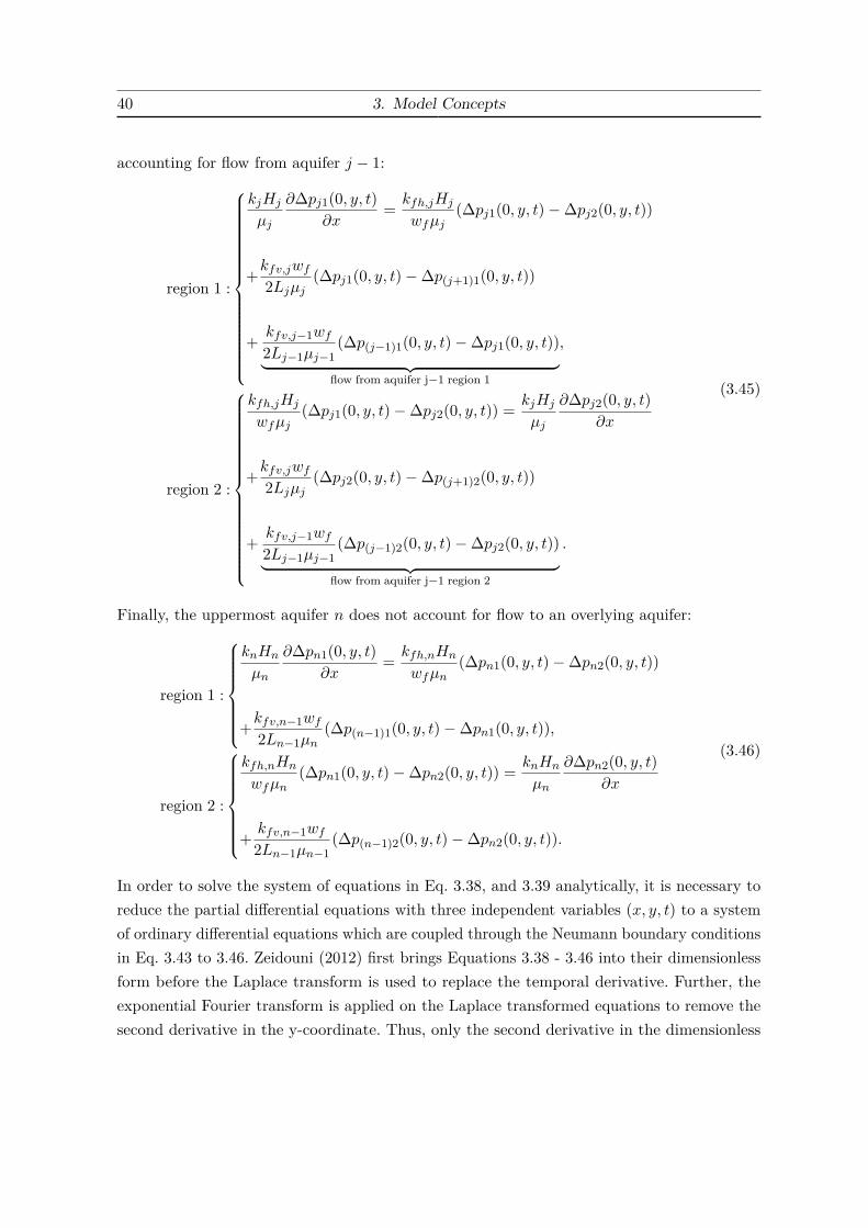
40 3. Model Concepts
accounting for flow from aquifer j − 1:
region 1 :
kjHj
µj
∂∆pj1(0, y, t)∂x
= kfh,jHj
wfµj(∆pj1(0, y, t)−∆pj2(0, y, t))
+kfv,jwf2Ljµj
(∆pj1(0, y, t)−∆p(j+1)1(0, y, t))
+ kfv,j−1wf2Lj−1µj−1
(∆p(j−1)1(0, y, t)−∆pj1(0, y, t))︸ ︷︷ ︸flow from aquifer j−1 region 1
,
region 2 :
kfh,jHj
wfµj(∆pj1(0, y, t)−∆pj2(0, y, t)) = kjHj
µj
∂∆pj2(0, y, t)∂x
+kfv,jwf2Ljµj
(∆pj2(0, y, t)−∆p(j+1)2(0, y, t))
+ kfv,j−1wf2Lj−1µj−1
(∆p(j−1)2(0, y, t)−∆pj2(0, y, t))︸ ︷︷ ︸flow from aquifer j−1 region 2
.
(3.45)
Finally, the uppermost aquifer n does not account for flow to an overlying aquifer:
region 1 :
knHn
µn
∂∆pn1(0, y, t)∂x
= kfh,nHn
wfµn(∆pn1(0, y, t)−∆pn2(0, y, t))
+kfv,n−1wf2Ln−1µn
(∆p(n−1)1(0, y, t)−∆pn1(0, y, t)),
region 2 :
kfh,nHn
wfµn(∆pn1(0, y, t)−∆pn2(0, y, t)) = knHn
µn
∂∆pn2(0, y, t)∂x
+ kfv,n−1wf2Ln−1µn−1
(∆p(n−1)2(0, y, t)−∆pn2(0, y, t)).
(3.46)
In order to solve the system of equations in Eq. 3.38, and 3.39 analytically, it is necessary toreduce the partial differential equations with three independent variables (x, y, t) to a systemof ordinary differential equations which are coupled through the Neumann boundary conditionsin Eq. 3.43 to 3.46. Zeidouni (2012) first brings Equations 3.38 - 3.46 into their dimensionlessform before the Laplace transform is used to replace the temporal derivative. Further, theexponential Fourier transform is applied on the Laplace transformed equations to remove thesecond derivative in the y-coordinate. Thus, only the second derivative in the dimensionless
3.2. Analytical Methods 41
Pressure for specific x, y, and t in each aquifer and region
Evaluation in theLaplace-Fourier domain
Governing equations for each aquifer
and region
System of dimensionless PDEs
Introduction of dimensionless terms
Sequential Laplace transform (time domain)
Laplace transformed equations
Exponential Fourier transform (space domain, y-coordinate)
Linear System of coupled ODEsLaplace and Fourier transformed
Coefficients for ODEs in the Laplace-Fourier domain
Fourier inversion(FFT in MATLAB)and Laplace inversion(Stehfest algorithm)
Figure 3.3.: Schematic overview of the solution procedure for the Zeidouni-Method, mod-ified after Scholz (2014). For numerically inverting the Laplace transform theStehfest algorithm is used (Stehfest, 1970).
x-coordinate remains, and the equations are reduced to a system of linear ordinary differentialequations. Once the transformed solution is found, it must be inverted in time and space. Thisis achieved numerically. An overview of the procedure is given in Fig. 3.3.
The main target variable of this model is usually not the resulting pressure distribution butrather the leakage rate into overlying aquifers. To calculate the leakage, for example into theuppermost aquifer, the following integral relation can be used:
Qleakage(t) = kfv,n−1wf2Ln−1µn−1
[ ∫ +∞
−∞(∆p(n−1)1(0, y, t)−∆pn1(0, y, t))dy
+∫ +∞
−∞(∆p(n−1)2(0, y, t)−∆pn2(0, y, t))dy
].
(3.47)
42 3. Model Concepts
In the implementation, finite integral boundaries have to be chosen for y, and the integral isreplaced by a sum, with N sampling steps and a sampling distance ∆y:
Qleakage(t) = kfv,n−1wf2Ln−1µn−1
2[N∑i=1
(∆p(n−1)1(i ·∆y − 12∆y)−∆pn1(i ·∆y − 1
2∆y))∆y
+N∑i=1
(∆p(n−1)2(i ·∆y − 12∆y)−∆pn2(i ·∆y − 1
2∆y))∆y].
(3.48)
Here, the constant values of x and t have been omitted, i.e. ∆p(y). Naturally, the integrationlength (N ·∆y) has to be chosen large enough such that the leakage rate is not significantlyinfluenced by a further extension of the integration domain. Evaluating the solution for toomany points can be computationally demanding. The factor of 2 in front of the sum arisesdue to the symmetry of the solution for y = 0.
3.3. Numerical Implementation
In this section, the numerical implementation of the different formulations given in Sec. 3.1.2is presented. All simulations are carried out with the numerical simulator DuMux. TheBox-Method is used for spatial discretization and the implicit Euler scheme is used fortemporal discretization. The Newton-Raphson method is used to solve the non-linear system ofequations. Additional implementations are required for the applications presented in this work.These include a 3D discrete-fracture approach for representing fault zones and infinite-aquiferboundary conditions achieved through a domain extension.
3.3.1. Numerical Simulator DuMux
All numerical models used in this work are implemented into the open-source numericalsimulator DuMux (Flemisch et al., 2011; Schwenck et al., 2015). DuMux stands for DUNEfor Multi-{Phase, Component, Scale, Physics,...} flow and transport in porous media. Thesimulator is based on the Distributed and Unified Numerics Environment (DUNE). It isan open-source system and has mainly been developed at the University of Stuttgart sinceJanuary 2007. DuMux is developed in C++ and provides a modular design which makes itideal for the implementation of porous-media model concepts. DuMux was used for a numberof problems in the field of CO2 storage in geological formations (Darcis et al., 2011; Walteret al., 2012, 2013; Kissinger et al., 2014) and was part of several code comparison studies(Nordbotten et al., 2012; Class et al., 2009).
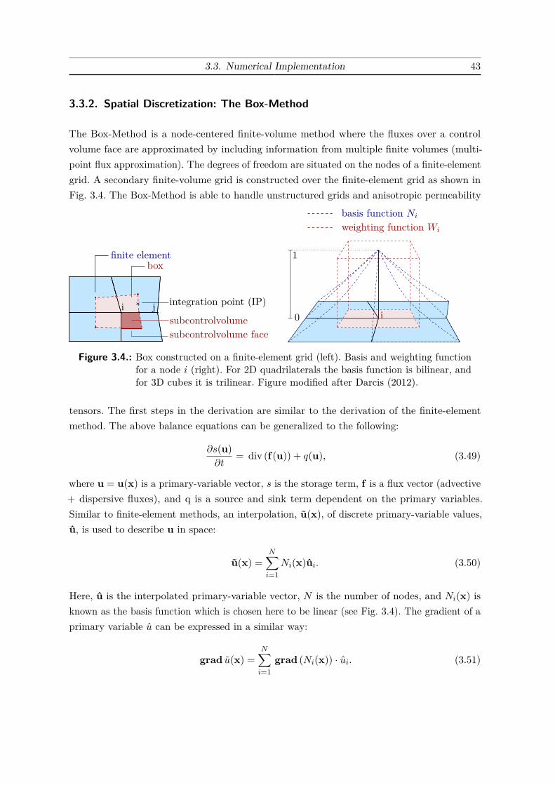
3.3. Numerical Implementation 43
3.3.2. Spatial Discretization: The Box-Method
The Box-Method is a node-centered finite-volume method where the fluxes over a controlvolume face are approximated by including information from multiple finite volumes (multi-point flux approximation). The degrees of freedom are situated on the nodes of a finite-elementgrid. A secondary finite-volume grid is constructed over the finite-element grid as shown inFig. 3.4. The Box-Method is able to handle unstructured grids and anisotropic permeability
weighting function Wi
basis function Ni
1
0 i
boxfinite element
subcontrolvolume face
integration point (IP)
subcontrolvolumei j
Figure 3.4.: Box constructed on a finite-element grid (left). Basis and weighting functionfor a node i (right). For 2D quadrilaterals the basis function is bilinear, andfor 3D cubes it is trilinear. Figure modified after Darcis (2012).
tensors. The first steps in the derivation are similar to the derivation of the finite-elementmethod. The above balance equations can be generalized to the following:
∂s(u)∂t
= div (f(u)) + q(u), (3.49)
where u = u(x) is a primary-variable vector, s is the storage term, f is a flux vector (advective+ dispersive fluxes), and q is a source and sink term dependent on the primary variables.Similar to finite-element methods, an interpolation, u(x), of discrete primary-variable values,u, is used to describe u in space:
u(x) =N∑i=1
Ni(x)ui. (3.50)
Here, u is the interpolated primary-variable vector, N is the number of nodes, and Ni(x) isknown as the basis function which is chosen here to be linear (see Fig. 3.4). The gradient of aprimary variable u can be expressed in a similar way:
grad u(x) =N∑i=1
grad (Ni(x)) · ui. (3.51)
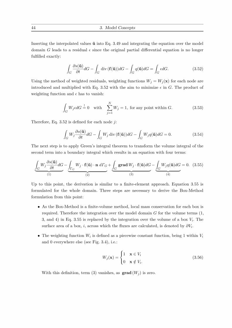
44 3. Model Concepts
Inserting the interpolated values u into Eq. 3.49 and integrating the equation over the modeldomain G leads to a residual ε since the original partial differential equation is no longerfulfilled exactly: ∫
G
∂s(u)∂t
dG−∫Gdiv (f(u))dG−
∫Gq(u)dG =
∫GεdG. (3.52)
Using the method of weighted residuals, weighting functions Wj = Wj(x) for each node areintroduced and multiplied with Eq. 3.52 with the aim to minimize ε in G. The product ofweighting function and ε has to vanish:
∫GWjεdG
!= 0 withN∑j=1
Wj = 1, for any point within G. (3.53)
Therefore, Eq. 3.52 is defined for each node j:∫GWj
∂s(u)∂t
dG−∫GWj div (f(u))dG−
∫GWjq(u)dG = 0. (3.54)
The next step is to apply Green’s integral theorem to transform the volume integral of thesecond term into a boundary integral which results in an equation with four terms:∫
GWj
∂s(u)∂t
dG︸ ︷︷ ︸(1)
−∫
ΓGWj · f(u) · n dΓG︸ ︷︷ ︸
(2)
+∫G
gradWj · f(u)dG︸ ︷︷ ︸(3)
−∫GWjq(u)dG︸ ︷︷ ︸
(4)
= 0. (3.55)
Up to this point, the derivation is similar to a finite-element approach. Equation 3.55 isformulated for the whole domain. Three steps are necessary to derive the Box-Methodformulation from this point:
• As the Box-Method is a finite-volume method, local mass conservation for each box isrequired. Therefore the integration over the model domain G for the volume terms (1,3, and 4) in Eq. 3.55 is replaced by the integration over the volume of a box Vi. Thesurface area of a box, i, across which the fluxes are calculated, is denoted by ∂Vi.
• The weighting function Wi is defined as a piecewise constant function, being 1 within Viand 0 everywhere else (see Fig. 3.4), i.e.:
Wj(x) =
1 x ∈ Vi0 x /∈ Vi.
(3.56)
With this definition, term (3) vanishes, as grad (Wj) is zero.

3.3. Numerical Implementation 45
• Mass lumping of the volume terms (1) and (4) is applied. This means that the massis stored only at the node, and therefore s(u) becomes s(ui), which is only dependenton the discrete primary-variable vector at the node, and can be written in front of theintegral, as it is no longer a function of space. The integral then simplifies to the volumeof the box Vi.
The balance equations for a finite volume or box at node i therefore become:
Vi∂s(ui)∂t
=∫∂Vi
f(u) · n dΓVi + Vi · q(ui). (3.57)
Note that the number of equations at a node i depends on the number of primary variables.The time derivative will be discretized in the next section. As for the flux term, it can besplit into an advective part and a dispersive part. The integral is replaced by a sum over thenumber of integration points at a node (ηIP,i):∫
∂Vi
f(u) · n dΓVi =∑
IP∈ηIP,i
(∑α
β(uupw)fa(uIP ) +∑α
fd(uIP ))· nIPAIP
with fa(uIP ) = − K(
grad (pα)IP − %αg)
and fd(uIP ) = − (%mα )IPDdisp grad (xκα)IP .
(3.58)
Here IP is the index of an integration point. Since discrete primary-variable values of uare not available at an integration point, the interpolated primary-variable values at thecoordinates of the integration point, i.e uIP or grad uIP , are interpolated using Eq. 3.50and 3.51. These interpolated values allow for the evaluation of the advective (fa) and thedispersive flux (fd) functions for each phase α. nIP and AIP are the outer normal vector andthe area of the sub-control volume face, respectively. In front of the advective-flux function,the term β(uupw) is the product of those parameters whose values require an upwinding inorder to avoid oscillations in advection dominated problems. In this work, a first order fullyupwind weighting function is used for all models. This means that the parameters within βare evaluated with the primary variables of the upstream node, i.e.
upw =
i fa · nij ≥ 0
j fa · nij < 0.(3.59)
Additionally, fa and fd both contain the permeability (K) and the hydromechanic dispersiontensor (Ddisp). For these parameters, a harmonic average is calculated at the integrationpoint, if the permeability and porosity are assigned at the node (box). If these properties areassigned on the element, no averaging is required. The density at the integration point within
46 3. Model Concepts
the Darcy velocity (%α) is the arithmetic mean of the adjacent nodes i and j.Neumann boundary conditions are evaluated within the flux term (Eq. 3.58). This means thatNeumann boundary fluxes are also allowed to be solution dependent, i.e. being a function ofuIP . Dirichlet boundary conditions at a node i are treated by replacing the balance equationfor a primary-variable vector ui with:
ui − uD = 0. (3.60)
Here, uD are the fixed Dirichlet values. Mixed boundary conditions for different primaryvariables at a node i are also possible.
3.3.3. Temporal Discretization: The Implicit Euler Scheme
To account for a general time discretization. the time differential ∂t is replaced by a finitedifference operator ∆t. Eq. 3.57 can be extended as:
Vis(un+1
i )∆tn − θ
∫∂Vi
f(un+1) · n dΓVi − Vi · q(un+1i )
−[Vis(uni )∆tn − (1− θ)
∫∂Vi
f(un) · n dΓVi − Vi · q(uni )]
= 0,(3.61)
where n denotes the time step index, and θ is a weighting coefficient (0 ≤ θ ≤ 1). θ = 0corresponds to an explicit scheme where all functions are evaluated with the primary variablesof the previous time step (n). θ = 1 yields the fully implicit scheme which is first order accuratein time (Helmig, 1997; Diersch and Kolditz, 2002) and unconditionally stable. In this work thefully implicit scheme is used for all numerical simulations. Equation 3.61 is rewritten here:
Vis(un+1
i )− s(uni )∆tn =
∫∂Vi
f(un+1) · n dΓVi + Vi · q(un+1i ). (3.62)
3.3.4. The Newton-Raphson Method
Equation 3.62 is generally non-linear, as the constitutive parameters, such as densities,viscosities, relative permeabilities etc. are all functions of the primary variables. In order tosolve a system of non-linear equations, an iterative scheme, such as the Newton-Raphsonmethod, applied in this work, can be used. First, Eq. 3.62 is reformulated into a residual form:
ri = Vis(un+1
i )− s(uni )∆tn −
∫∂Vi
f(un+1) · n dΓVi − Vi · q(un+1i ). (3.63)
3.3. Numerical Implementation 47
For a system with N nodes and P primary variables per node, the resulting number ofequations is N × P . The Jacobian matrix J is obtained by forming partial derivatives of eachequation ri with respect to each connected primary variable uj . The partial derivatives for Jare calculated numerically. The linearized equation system for the Newton-Raphson method is:
J(uk)∆uk = r(uk) (3.64)
with ∆uk = uk+1 − uk,
where the time step index is omitted and the iteration index k is introduced. The iterationis repeated until a convergence criterion is fulfilled. A convergence criterion can be an errornorm such as the L2 norm applied on the residual vector, or the prescribed demand for severaldigits accuracy in the calculated primary variables. The latter approach is used in this work,and is formulated in the following manner:
ε > max
(∆uk1
0.5(uk+11 + uk1)
, ...,∆ukN
0.5(uk+1N + ukN )
). (3.65)
The Newton-Raphson method is described in more detail for multi-phase flow problems inHelmig (1997).
3.3.5. Fault-Zone Representation Using a Discrete-Fracture Approach
The implementation of a discrete-fracture model on top of the existing models discretized withthe Box-Method is shown here. In the context of this work it is used for the representation offault zones.In the application presented in Chapter 5, complex multi-layer geological systems have to bediscretized. The grids used for these kinds of systems are usually horizontally aligned with thegeological layers. However, there are vertical discontinuities such as fault zones or salt domeswhich can play a crucial role for the flow field, as they can be impermeable or permeable tohorizontal or vertical flow. Fault zones can be considered as planar discontinuities, where theirwidth is much smaller than their height or length. In large-scale models, the width of a faultzone can therefore be much smaller than the horizontal discretization length. Describing afault zone in detail would require severe grid refinement, not only leading to an increasedcomputational effort but also requiring additional work during the grid generation. In orderto avoid this grid refinement but still be able to describe the relevant characteristics of afault zone, a discrete-fracture approach is implemented. Within this approach a fractureor fault zone can be described with three parameters: fracture width, fracture permeabilityand fracture porosity. Fig. 3.5 shows the discretization of a fault zone in a horizontal layer.
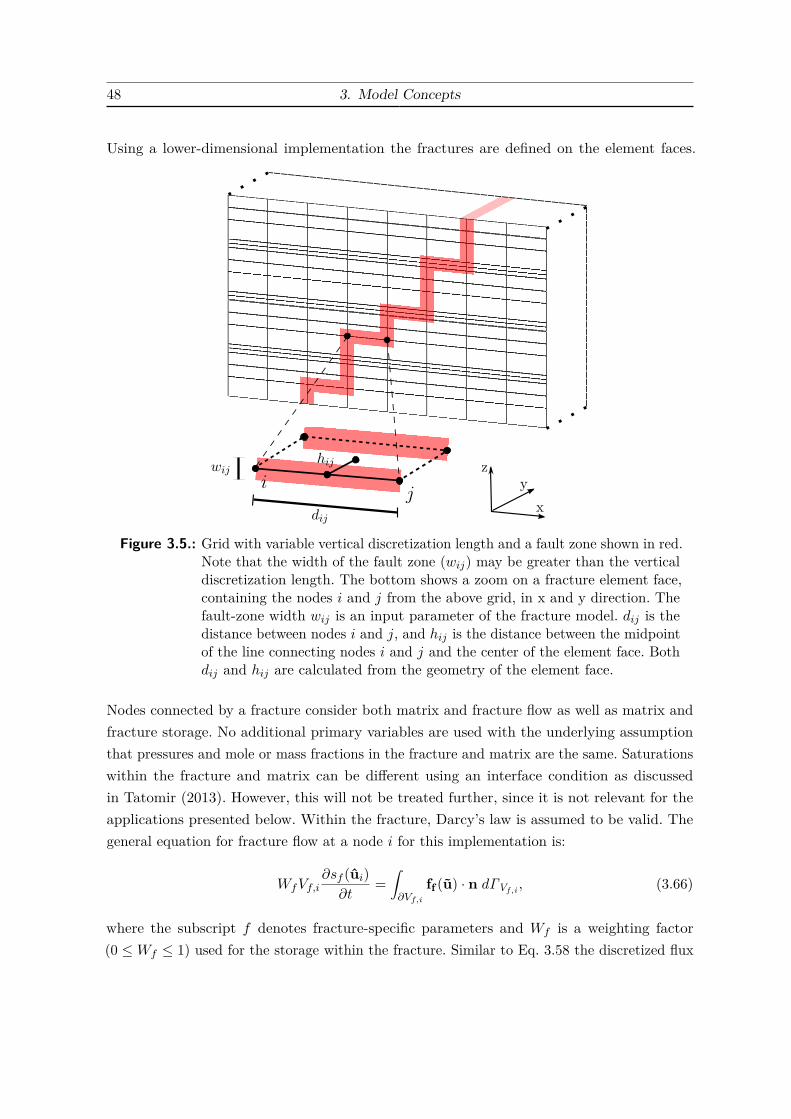
48 3. Model Concepts
Using a lower-dimensional implementation the fractures are defined on the element faces.
dij
wijhij z
xyi
j
Figure 3.5.: Grid with variable vertical discretization length and a fault zone shown in red.Note that the width of the fault zone (wij) may be greater than the verticaldiscretization length. The bottom shows a zoom on a fracture element face,containing the nodes i and j from the above grid, in x and y direction. Thefault-zone width wij is an input parameter of the fracture model. dij is thedistance between nodes i and j, and hij is the distance between the midpointof the line connecting nodes i and j and the center of the element face. Bothdij and hij are calculated from the geometry of the element face.
Nodes connected by a fracture consider both matrix and fracture flow as well as matrix andfracture storage. No additional primary variables are used with the underlying assumptionthat pressures and mole or mass fractions in the fracture and matrix are the same. Saturationswithin the fracture and matrix can be different using an interface condition as discussedin Tatomir (2013). However, this will not be treated further, since it is not relevant for theapplications presented below. Within the fracture, Darcy’s law is assumed to be valid. Thegeneral equation for fracture flow at a node i for this implementation is:
WfVf,i∂sf (ui)∂t
=∫∂Vf,i
ff (u) · n dΓVf ,i , (3.66)
where the subscript f denotes fracture-specific parameters and Wf is a weighting factor(0 ≤Wf ≤ 1) used for the storage within the fracture. Similar to Eq. 3.58 the discretized flux
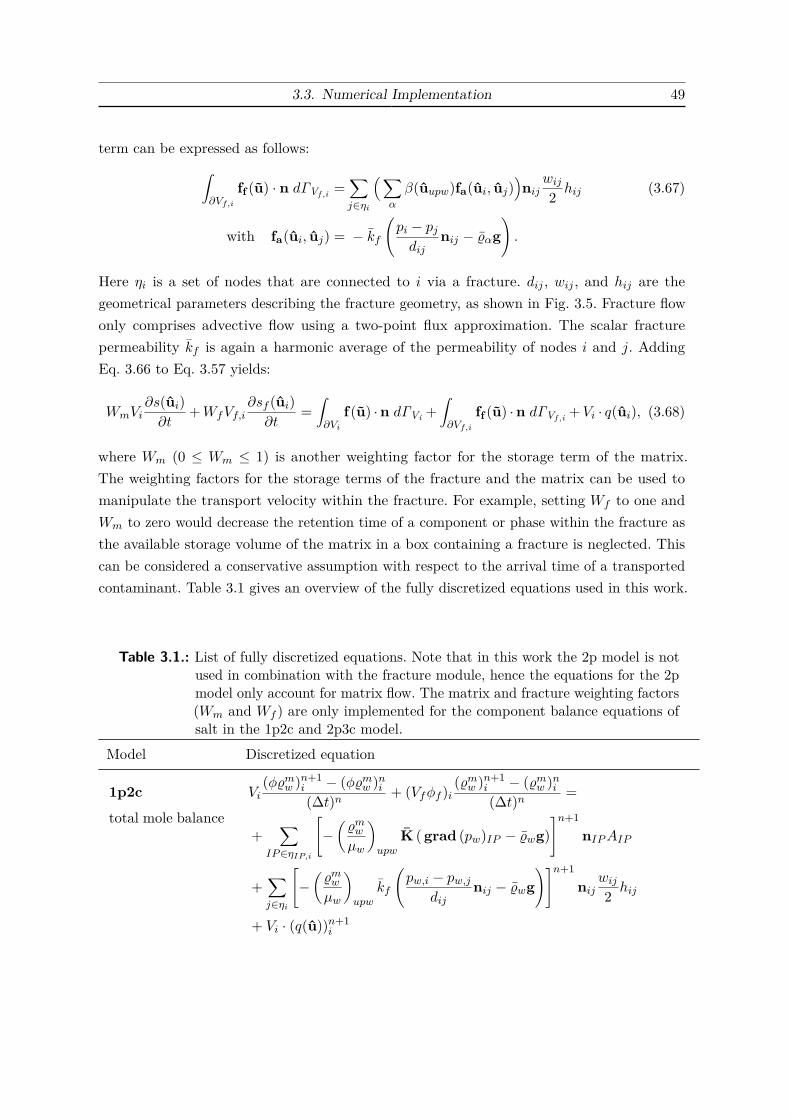
3.3. Numerical Implementation 49
term can be expressed as follows:∫∂Vf,i
ff (u) · n dΓVf ,i =∑j∈ηi
(∑α
β(uupw)fa(ui, uj))nij
wij2 hij (3.67)
with fa(ui, uj) = − kf(pi − pjdij
nij − %αg).
Here ηi is a set of nodes that are connected to i via a fracture. dij , wij , and hij are thegeometrical parameters describing the fracture geometry, as shown in Fig. 3.5. Fracture flowonly comprises advective flow using a two-point flux approximation. The scalar fracturepermeability kf is again a harmonic average of the permeability of nodes i and j. AddingEq. 3.66 to Eq. 3.57 yields:
WmVi∂s(ui)∂t
+WfVf,i∂sf (ui)∂t
=∫∂Vi
f(u) ·n dΓVi +∫∂Vf,i
ff (u) ·n dΓVf ,i +Vi · q(ui), (3.68)
where Wm (0 ≤ Wm ≤ 1) is another weighting factor for the storage term of the matrix.The weighting factors for the storage terms of the fracture and the matrix can be used tomanipulate the transport velocity within the fracture. For example, setting Wf to one andWm to zero would decrease the retention time of a component or phase within the fracture asthe available storage volume of the matrix in a box containing a fracture is neglected. Thiscan be considered a conservative assumption with respect to the arrival time of a transportedcontaminant. Table 3.1 gives an overview of the fully discretized equations used in this work.
Table 3.1.: List of fully discretized equations. Note that in this work the 2p model is notused in combination with the fracture module, hence the equations for the 2pmodel only account for matrix flow. The matrix and fracture weighting factors(Wm and Wf ) are only implemented for the component balance equations ofsalt in the 1p2c and 2p3c model.
Model Discretized equation
1p2c
total mole balance
Vi(φ%mw )n+1
i − (φ%mw )ni(∆t)n + (Vfφf )i
(%mw )n+1i − (%mw )ni(∆t)n =
+∑
IP∈ηIP,i
[−(%mwµw
)upw
K ( grad (pw)IP − %wg)]n+1
nIPAIP
+∑j∈ηi
[−(%mwµw
)upw
kf
(pw,i − pw,j
dijnij − %wg
)]n+1
nijwij2 hij
+ Vi · (q(u))n+1i

50 3. Model Concepts
Table 3.1.: List of fully discretized equations. Note that in this work the 2p model is notused in combination with the fracture module, hence the equations for the 2pmodel only account for matrix flow. The matrix and fracture weighting factors(Wm and Wf ) are only implemented for the component balance equations ofsalt in the 1p2c and 2p3c model.
Model Discretized equation
1p2c
component balance
salt
WmVi(φ%mw xSw)n+1
i − (φ%mw xSw)ni(∆t)n +Wf (Vfφf )i
(%mw xSw)n+1i − (%mw xSw)ni(∆t)n =
+∑
IP∈ηIP,i
[−(%mw x
Sw
µw
)upw
K ( grad (pw)IP − %wg)
− (%mw )IP DSw,pm grad (xSw)IP
]n+1
nIPAIP
+∑j∈ηi
−(%mw xSwµw
)upw
kf
(pw,i − pw,j
dijnij − %wαg
)n+1
nijwij2 hij
+ Vi · (q(u))n+1i
primary variables u : pw, xSw
2p
phase balance
α = brine or CO2
Vi(φ%αSα)n+1
i − (φ%αSα)ni(∆t)n =
+∑
IP∈ηIP,i
[−(%αkrαµα
)upw
K ( grad (pα)IP − %αg)]n+1
nIPAIP
+ Vi · (qα(u))n+1i
primary variables u : pw, Sn

3.3. Numerical Implementation 51
Table 3.1.: List of fully discretized equations. Note that in this work the 2p model is notused in combination with the fracture module, hence the equations for the 2pmodel only account for matrix flow. The matrix and fracture weighting factors(Wm and Wf ) are only implemented for the component balance equations ofsalt in the 1p2c and 2p3c model.
Model Discretized equation
2p3c
component balance
κ = H2O or CO2
Vi
∑α
(φ%mα Sαx
κα)n+1i − (φ%mα Sαxκα)ni
)(∆t)n
+ (Vfφf )i
∑α
((%mα Sαxκα)n+1
i − (%mα Sαxκα)ni)
(∆t)n =
+∑
IP∈ηIP,i
[∑α
(−(%mα krαx
κα
µα
)upw
K ( grad (pα)IP − %αg))
−∑α
(− (%mα )IP Dκ
α,pm grad (xκα)IP)]n+1
nIPAIP
+∑j∈ηi
[−(%mα x
κα
µα
)upw
kf
(pα,i − pα,j
dijnij − %αg
)]n+1
nijwij2 hij
+ Vi · (qκ(u))n+1i
2p3c
component balance
κ = salt
WmVi
∑α
(φ%mα Sαx
κα)n+1i − (φ%mα Sαxκα)ni
)(∆t)n
+Wf (Vfφf )i
∑α
((%mα Sαxκα)n+1
i − (%mα Sαxκα)ni)
(∆t)n =
+∑
IP∈ηIP,i
[∑α
(−(%mα krαx
κα
µα
)upw
K ( grad (pα)IP − %αg))
−∑α
(− (%mα )IP Dκ
α,pm grad (xκα)IP)]n+1
nIPAIP
+∑j∈ηi
[−(%mα x
κα
µα
)upw
kf
(pα,i − pα,j
dijnij − %αg
)]n+1
nijwij2 hij
+ Vi · (qκ(u))n+1i
primary variables u : pw, Sn/xCO2w /xH2O
n , xSw
The 3D implementation of the discrete-fracture approach is done in a general way to ensurethat it can easily be coupled to the different model types (1p2c, 2p, 2p3c) used in this work.It is therefore an extension and generalization of the implementation by Tatomir (2013) which
52 3. Model Concepts
is 2D and specific to the 2p model in DuMux. Additionally, the implementation is valid fordifferent element types, such as simplex or hexahedral grids.
An alternative approach to the representation of fault zones that avoids refinement could bean upscaling procedure coming from a fine grid fully describing the geometry of the fault zone,for example, a multiple interacting continua (MINC) approach, as described in Tatomir (2013).However, some effort is required as well to implement a generalized method for converting thecomplex geometrical information of the fault zone into effective parameters.
3.3.6. Infinite-Aquifer Boundary Conditions
Another necessary implementation for this work is the extension of an arbitrary domain,henceforth called the inner domain, by an outer domain. This outer domain extends to acertain radius, ensuring that the pressure buildup within the inner domain is not underestimateddue to its boundaries being too close to the injection point.
A saline aquifer confined by barrier layers on top and bottom is generally characterized bylateral dimensions much larger than the vertical ones. During the injection of CO2 into suchan aquifer, the lateral extent, that is subject to pressure increases is much larger than thelateral extent of the CO2 plume. Models primarily concerned with the shape and fate of theCO2 plume often use Dirichlet boundary conditions for pressure on the lateral boundaries atdistances too small, such that the actual pressure buildup would reach further than the modelboundaries. This means that the resistance to lateral flow is reduced and the pressures thatevolve are underestimated. When predicting the CO2-plume shape, this usually does not posea significant problem. However, if the primary aim of the model is characterizing brine flowat large distances from the injection point, as will be the case in Chapter 5, lateral Dirichletboundary conditions will lead to an underestimation of the vertical migration of brine throughvertical discontinuities in the barrier layers.
As far-field information of saline aquifers is usually sparse, assumptions have to be made. Onepossible assumption is an infinite extent of the aquifer. This means that the pressure at infinitedistance from the injection remains unchanged. In this work, this condition is approximatedby extending the model domain (inner domain) by a circular outer domain with a coarser grid.The discretization length of the outer domain may increase as a function of the radius. Anexample of an inner and an outer domain is given in Fig. 3.6. As the discretization length ofthe outer domain can be chosen much coarser, the additional computational demand can bekept within reasonable limits. The effect on the results however is significant, as will be shownin Chapter 5.
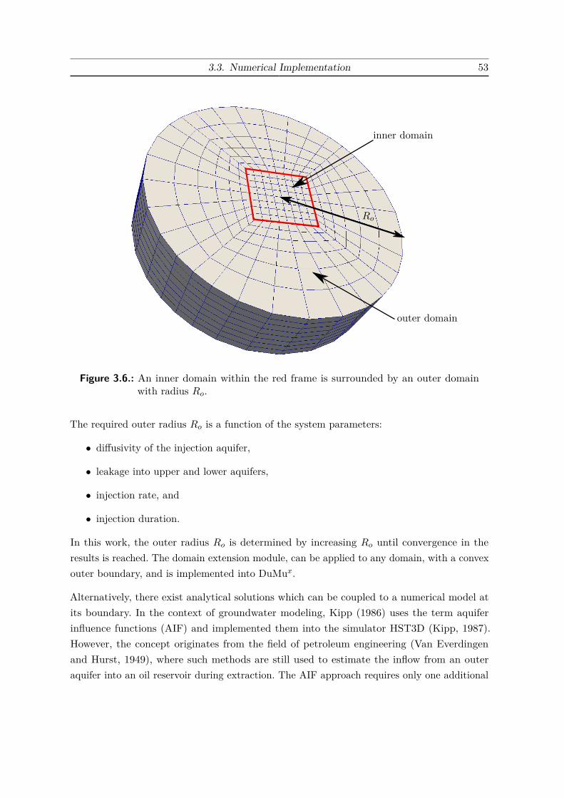
3.3. Numerical Implementation 53
outer domain
inner domain
Ro
Figure 3.6.: An inner domain within the red frame is surrounded by an outer domainwith radius Ro.
The required outer radius Ro is a function of the system parameters:
• diffusivity of the injection aquifer,
• leakage into upper and lower aquifers,
• injection rate, and
• injection duration.
In this work, the outer radius Ro is determined by increasing Ro until convergence in theresults is reached. The domain extension module, can be applied to any domain, with a convexouter boundary, and is implemented into DuMux.
Alternatively, there exist analytical solutions which can be coupled to a numerical model atits boundary. In the context of groundwater modeling, Kipp (1986) uses the term aquiferinfluence functions (AIF) and implemented them into the simulator HST3D (Kipp, 1987).However, the concept originates from the field of petroleum engineering (Van Everdingenand Hurst, 1949), where such methods are still used to estimate the inflow from an outeraquifer into an oil reservoir during extraction. The AIF approach requires only one additional

54 3. Model Concepts
primary variable per boundary node. However, the assumptions made are more severe, asthe underlying analytical model was developed for a circular domain, putting restrictions onarbitrary inner model shapes as well as stratified aquifer systems.
4. Basin-Scale Screening for CO2 StorageEfficiency1
This chapter deals with a screening method for determining suitable areas for CO2 storagebased on their storage efficiency. The storage efficiency is a measure of how efficient a reservoircan be utilized. In literature (e.g. Okwen et al. (2010)), the term storage efficiency is oftendefined as the volume of injected CO2 divided by the pore space (see Eq. 3.35), which isreferred to here as volumetric storage efficiency. However, in this work the storage efficiencyis defined in terms of the mass of CO2 in place, which is the target variable used here forcomparing different reservoirs. The database used for the screening covers regionalized data fordepth, temperature conditions and salt concentrations of the Middle Buntsandstein rock unitin the North German Basin. As proposed by Kopp et al. (2009a), the gravitational number,Gr (see Eq. 3.19), is used as a qualitative indicator for storage efficiency to determine more orless favorable areas for CO2 injection. Unfortunately, a reservoir database similar to the U.S.National Petroleum Council public database (NPC, 1984) used by Kopp et al. (2009a,b) is notavailable for the North German Basin. No regionalized data for the permeability, the porosityand the reservoir thickness are available. However, the initial fluid properties (viscosities anddensities of brine and CO2) can be estimated from measured depth contours, temperatureprofiles, and salt concentrations.In Sec 4.1, the relevant driving forces influencing storage efficiency are explained. The availabledatabase is described in Sec. 4.2, followed by a description of the numerical model’s setup inSec. 4.3. Results of the regional calculation of the Gravitational Number (Gr) for the MiddleBuntsandstein rock unit are presented in Sec. 4.4.1. Based on these results, several data pointsof the database are selected for more detailed numerical investigations with the aim of:
• quantifying the impact of varying depths, temperature conditions, and salt concentrationsin the Middle Buntsandstein on storage efficiency (Sec. 4.4.2),
• testing the Gr-criterion as a qualitative screening criterion for storage efficiency and com-paring the results to the screening method proposed by Okwen et al. (2010) (Sec. 4.4.2),
1The main parts of this chapter have been published in Kissinger et al. (2014).
56 4. Basin-Scale Screening for CO2 Storage Efficiency
• investigating the effect of Gr-criterion on the amount of residually trapped CO2 (Sec. 4.4.3).
Moreover, in Sec. 4.4.4, three different regions are selected which are characterized by differentvalues of Gr (high, medium, and low). For these regions, published data for reservoir thicknessand porosity are gathered as input for the numerical simulations. The aim of these simulationsis to check:
• if Gr, based on the initial fluid properties, has a recognizable effect on storage efficiencywhen area-specific distributions of reservoir thickness and porosity are considered aswell.
4.1. The Gravitational Number as a Qualitative Indicator forStorage Efficiency
In an injection scenario, where CO2 is injected via a vertical injection well into residentbrine held in a confined homogeneous reservoir, the CO2 plume shape is characterized by thefollowing driving forces:
• Viscous forces (or advective forces). The injection causes a displacement of resident brineaway from the injection well.
• Gravitational (or buoyant forces). Due to the density difference between the two fluidphases, an upward flow of the lighter CO2 phase is induced (gravity segregation) as wellas horizontal flow of the CO2 phase along the cap-rock due to a horizontal pressuregradient at the tip of the CO2 tongue (buoyant drive).
• Capillary forces. Capillary pressure gradients lead to the development of a capillary fringeat the interface between the two phases depending on the capillary pressure-saturationrelationship.
The influence of these driving forces and especially the ratio of gravitational to advective forceshas been investigated in many subsurface applications. Examples include: steam injection intooil reservoirs (Rapoport, 1955; Lookeren, 1983; Li and Lake, 1995), steam injection into fullywater-saturated porous media in the context of soil remediation (Ochs et al., 2010), or CO2
storage (Nordbotten and Celia, 2006, 2012; Nazarian et al., 2013; Taku Ide et al., 2007; Koppet al., 2010). Also, other related subsurface applications, like geothermal systems (cold waterinjection) or the storage of methane in subsurface formations, have similarities, where theratios between their driving forces help to describe the spreading behavior of the injected fluid.There are many established dimensionless groups that are useful in the characterization of a
4.1. The Gravitational Number as a Qualitative Indicator for Storage Efficiency 57
reservoir (Rapoport, 1955; Li and Lake, 1995; Zhou et al., 1997).In the context of CO2 injection, Kopp et al. (2009a) define the dimensionless capillary number(Ca) and the gravitational number (Gr) using a fractional flow formulation, as presented inSec. 3.1.2, and shown here again. The Capillary Number is defined as:
Ca = kpcrµnvcrlcr
= capillary forcesviscous forces . (4.1)
Further, the Gravitational Number is defined as:
Gr = (%w − %n)gkµnvcr
= gravitational forcesviscous forces , (4.2)
where k is the scalar intrinsic permeability, pcr is a characteristic capillary pressure, µn is thedynamic viscosity of CO2, lcr is a characteristic length of the system, vcr is a characteristicDarcy velocity, %w is the brine density, %n is the CO2 density and g is the acceleration dueto gravity. Kopp et al. (2009a) suggest using Ca and Gr for qualitatively ranking differentreservoirs according to their storage efficiency. Through numerical simulations, they showthat advective forces, dominating over gravitational forces (small values of Gr), and capillaryforces, dominating over advective forces (large values of Ca), lead to a higher storage efficiency.They further conclude that Gr has a stronger influence on storage efficiency than Ca for largesystem dimensions. This conclusion is also confirmed by Nordbotten and Celia (2012) whoscale capillary pressure with the hydrostatic pressure difference within a formation. Theyshow that capillary pressure generally reduces the saturation of the CO2 front with increasingdistance from the well. This reduction, is caused by a smearing of the front, following adiffusion-like behavior, leading to a reduced plume velocity at the tip, and therefore a higherstorage efficiency. Nordbotten and Celia (2012) conclude that if the capillary fringe is smallcompared to the thickness of the reservoir, capillary forces can be neglected and the assumptionof a sharp interface model becomes reasonable. In this work, Ca will not be considered in theestimation of storage efficiency since the database used does not allow for any reliable regionaldifferentiation of capillary pressure-saturation relationships.In this work Gr is used as a qualitative indicator for storage efficiency, as concluded by Koppet al. (2009a,b). The ratio between gravitational and advective forces is not constant. Near theinjection well advective forces dominate, but with increasing distance from the injection wellthe advective forces decrease. Thus, sooner or later the two phases will separate and the CO2
plume will then spread mainly underneath the top of the reservoir. Close to the injection well,where the advective forces are high (i.e. high vcr, see Eq. 4.2), the plume spreads cylindrically.Kopp et al. (2009a) calculate the characteristic velocity vcr in Eq. 4.2 from an average timedependent velocity obtained from simulation results. As this is not an option for the largedata set of this study, a priori estimate of vcr is defined, characteristic for the advective forces
58 4. Basin-Scale Screening for CO2 Storage Efficiency
in the system. For this purpose the specific volumetric injection rate mn%n
is used, where mn isthe specific mass injection rate of CO2 (i.e. the injection rate divided by the area of the well)in [kg/s/m2]. This results in the following definition of Gr:
Gr = (%w − %n)gkµn
mn%n
. (4.3)
The smaller the priorly calculated Gravitational Number (Eq. 4.3), the more the advectiveforces will dominate over the gravitational forces, which leads to a more piston-like displacement.As a result, the storage efficiency is increased, as the CO2 spreads over a larger fraction of thereservoir. Besides increasing the storage efficiency also the amount of residually trapped CO2
increases, which is beneficial for storage safety. The effect of Gr on residual trapping was alsoshown by Taku Ide et al. (2007).Since there are no data for permeability (k) and the actual specific injection rate (mCO2) usedis not known beforehand, these two parameters are set to 1 in order to make it clear that theyare not varied in the calculation of the a priori Gr.As shown in the derivation of the sharp interface model (Eq. 3.30) and the Okwen-Method(Eq. 3.37) the mobility ratio λ is an important factor in the estimation of storage efficiency.When using Gr, as defined in Eq. 4.3, to qualitatively compare different locations, the influenceof the brine mobility and therefore the spatial variability of the brine viscosity is neglected.To see if this is a valid assumption, the results are compared to the Okwen-Method, whichis explained in detail in Sec. 3.2.1. The main equation for estimating the volumetric storageefficiency E = Vinjected
Vformation, based on the mobility ratio λ and the gravitational number Γ, is
presented here again:
E = (1− Srw) 1λ
0 ≤ Γ < 0.5,
E = 2(1− Srw)(0.0324λ− 0.0952)Γ + (0.1778λ+ 5.9682)Γ1/2 + 1.6962λ− 3.0472
, (4.4)
0.5 ≤ Γ ≤ 50.
Γ is another definition of the gravitational number defined as:
Γ = 2π∆%gkλwH2
Qwell, (4.5)
where H is the reservoir thickness and Qwell is the volumetric injection rate. λ and λw can besimplified to µw
µnand 1
µwrespectively, when assuming that the relative permeability of brine
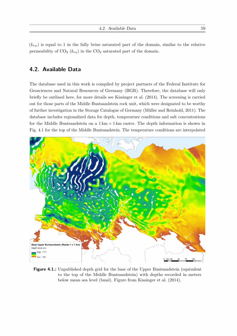
4.2. Available Data 59
(krw) is equal to 1 in the fully brine saturated part of the domain, similar to the relativepermeability of CO2 (krn) in the CO2 saturated part of the domain.
4.2. Available Data
The database used in this work is compiled by project partners of the Federal Institute forGeosciences and Natural Resources of Germany (BGR). Therefore, the database will onlybriefly be outlined here, for more details see Kissinger et al. (2014). The screening is carriedout for those parts of the Middle Buntsandstein rock unit, which were designated to be worthyof further investigation in the Storage Catalogue of Germany (Müller and Reinhold, 2011). Thedatabase includes regionalized data for depth, temperature conditions and salt concentrationsfor the Middle Buntsandstein on a 1 km× 1 km raster. The depth information is shown inFig. 4.1 for the top of the Middle Buntsandstein. The temperature conditions are interpolated
Figure 4.1.: Unpublished depth grid for the base of the Upper Buntsandstein (equivalentto the top of the Middle Buntsandstein) with depths recorded in metersbelow mean sea level (bmsl). Figure from Kissinger et al. (2014).
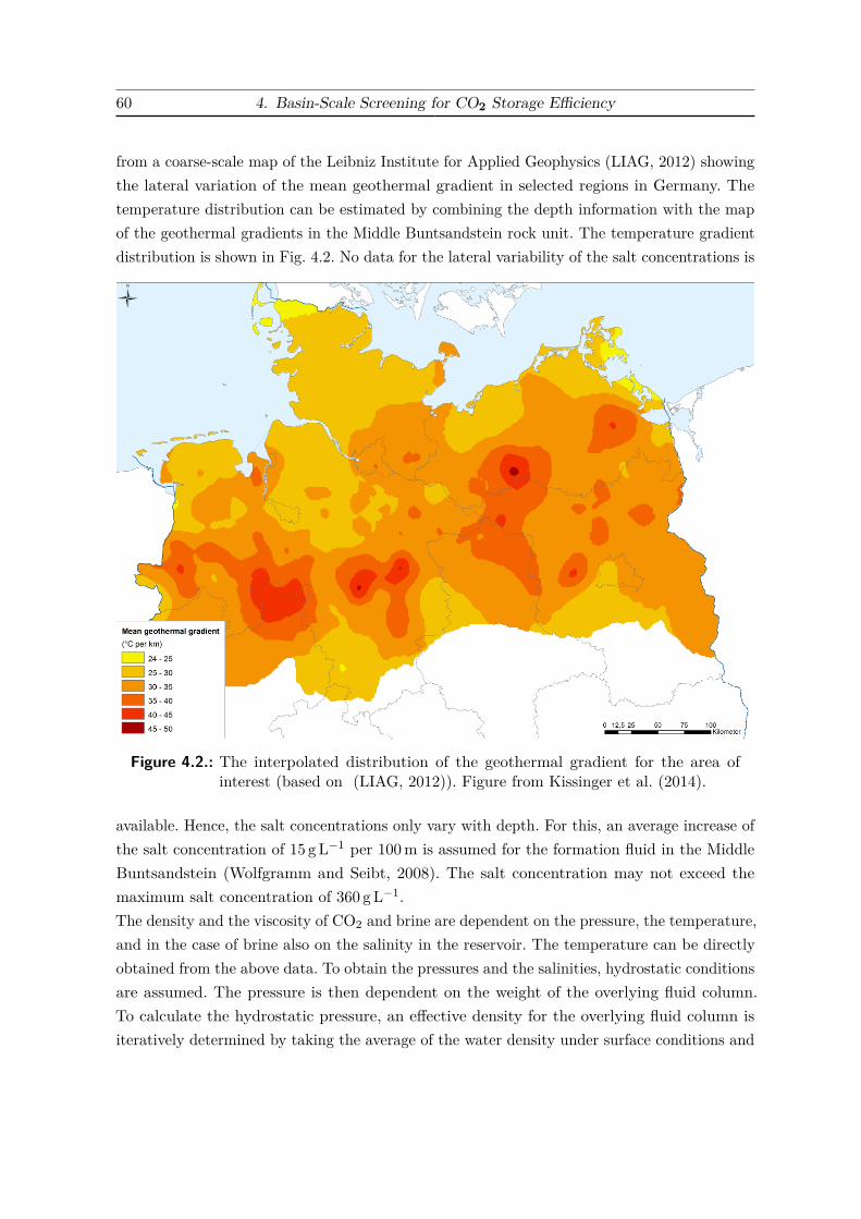
60 4. Basin-Scale Screening for CO2 Storage Efficiency
from a coarse-scale map of the Leibniz Institute for Applied Geophysics (LIAG, 2012) showingthe lateral variation of the mean geothermal gradient in selected regions in Germany. Thetemperature distribution can be estimated by combining the depth information with the mapof the geothermal gradients in the Middle Buntsandstein rock unit. The temperature gradientdistribution is shown in Fig. 4.2. No data for the lateral variability of the salt concentrations is
Figure 4.2.: The interpolated distribution of the geothermal gradient for the area ofinterest (based on (LIAG, 2012)). Figure from Kissinger et al. (2014).
available. Hence, the salt concentrations only vary with depth. For this, an average increase ofthe salt concentration of 15 gL−1 per 100m is assumed for the formation fluid in the MiddleBuntsandstein (Wolfgramm and Seibt, 2008). The salt concentration may not exceed themaximum salt concentration of 360 gL−1.The density and the viscosity of CO2 and brine are dependent on the pressure, the temperature,and in the case of brine also on the salinity in the reservoir. The temperature can be directlyobtained from the above data. To obtain the pressures and the salinities, hydrostatic conditionsare assumed. The pressure is then dependent on the weight of the overlying fluid column.To calculate the hydrostatic pressure, an effective density for the overlying fluid column isiteratively determined by taking the average of the water density under surface conditions and

4.2. Available Data 61
the brine density in the reservoir, which is a function of salinity, temperature and pressure. Asthe actual pressures are unknown, this is assumed to be a reasonable estimate. The salinitycan thus also be determined from the calculated brine density in the reservoir and the saltconcentration at each data point. Figure 4.3 shows the fluid properties of CO2 and brine,as well as the data points of the database plotted over the independent variables pressure,temperature and salinity. With the calculated values of viscosity and density the gravitationalnumber can be obtained using Eq. 4.3 for each data point. As explained in Sec. 4.1 thepermeability and the specific injection rate are not varied in this calculation, and are thereforeset to 1.
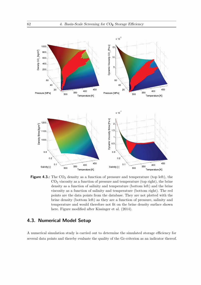
62 4. Basin-Scale Screening for CO2 Storage Efficiency
Figure 4.3.: The CO2 density as a function of pressure and temperature (top left), theCO2 viscosity as a function of pressure and temperature (top right), the brinedensity as a function of salinity and temperature (bottom left) and the brineviscosity as a function of salinity and temperature (bottom right). The redpoints are the data points from the database. They are not plotted with thebrine density (bottom left) as they are a function of pressure, salinity andtemperature and would therefore not fit on the brine density surface shownhere. Figure modified after Kissinger et al. (2014).
4.3. Numerical Model Setup
A numerical simulation study is carried out to determine the simulated storage efficiency forseveral data points and thereby evaluate the quality of the Gr-criterion as an indicator thereof.
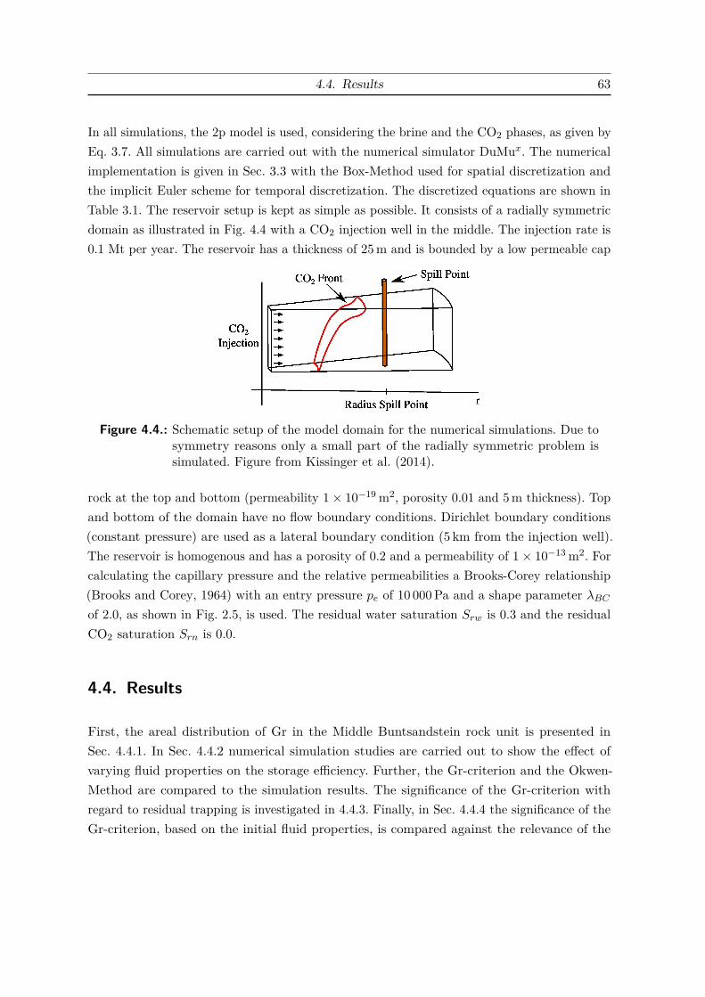
4.4. Results 63
In all simulations, the 2p model is used, considering the brine and the CO2 phases, as given byEq. 3.7. All simulations are carried out with the numerical simulator DuMux. The numericalimplementation is given in Sec. 3.3 with the Box-Method used for spatial discretization andthe implicit Euler scheme for temporal discretization. The discretized equations are shown inTable 3.1. The reservoir setup is kept as simple as possible. It consists of a radially symmetricdomain as illustrated in Fig. 4.4 with a CO2 injection well in the middle. The injection rate is0.1 Mt per year. The reservoir has a thickness of 25m and is bounded by a low permeable cap
Figure 4.4.: Schematic setup of the model domain for the numerical simulations. Due tosymmetry reasons only a small part of the radially symmetric problem issimulated. Figure from Kissinger et al. (2014).
rock at the top and bottom (permeability 1× 10⁻¹⁹ m2, porosity 0.01 and 5m thickness). Topand bottom of the domain have no flow boundary conditions. Dirichlet boundary conditions(constant pressure) are used as a lateral boundary condition (5 km from the injection well).The reservoir is homogenous and has a porosity of 0.2 and a permeability of 1× 10⁻¹³ m2. Forcalculating the capillary pressure and the relative permeabilities a Brooks-Corey relationship(Brooks and Corey, 1964) with an entry pressure pe of 10 000Pa and a shape parameter λBCof 2.0, as shown in Fig. 2.5, is used. The residual water saturation Srw is 0.3 and the residualCO2 saturation Srn is 0.0.
4.4. Results
First, the areal distribution of Gr in the Middle Buntsandstein rock unit is presented inSec. 4.4.1. In Sec. 4.4.2 numerical simulation studies are carried out to show the effect ofvarying fluid properties on the storage efficiency. Further, the Gr-criterion and the Okwen-Method are compared to the simulation results. The significance of the Gr-criterion withregard to residual trapping is investigated in 4.4.3. Finally, in Sec. 4.4.4 the significance of theGr-criterion, based on the initial fluid properties, is compared against the relevance of the

64 4. Basin-Scale Screening for CO2 Storage Efficiency
parameters porosity and reservoir thickness for three areas, with a high, medium, and lowvalue of Gr.
4.4.1. Basin-Scale Application of the Gravitational Number
The calculated values of Gr vary from around 4× 10¹⁰ to 1× 10¹¹. To display the results ina map, these values have been divided into six classes, as shown in Fig. 4.5. Areas with lowvalues of Gr are assumed to be indicative of a high storage efficiency and are depicted in lightgreen. On the other hand, areas with high values of Gr are assumed to be indicative of a lowstorage efficiency and are depicted in red.A comparison between the resulting Gr distribution (Fig. 4.5) with the regional geothermalgradient variations (Fig. 4.2), and the rock unit depths (Fig. 4.1) shows that for areas withshallow to medium depths (800–2000m), the values of Gr are mainly affected by variations inthe geothermal gradient. Thus, low geothermal gradients result in small Gr values whereashigh geothermal gradients result in high Gr values. A similar observation can be made for areaswith greater depths (2000–4000m). However, this relation is slightly less pronounced than forthe shallow to medium depths. For depths >4000m, low values of Gr are predominant.At depths between 800–4000m, assuming that conditions are not close to or below the criticalpoint of CO2, only a moderate increase in CO2 density and viscosity is observed over depth.Both the CO2 density and the viscosity increase with increasing pressure and decrease withincreasing temperature. For an increasing depth the influence of the pressure increase slightlyoutweighs the influence of the temperature increase. This causes only a moderate reduction ofGr over depth, and strongly relates the values of Gr to the lateral variations in the geothermalgradient.
4.4.2. Comparison of the Gr-Criterion and the Okwen-Method with Respect toStorage Efficiency
For the simulations, different representative data points are chosen which cover various depthsand the full range of Gr values. These data points provide the conditions (pressure, temperatureand salinity) upon which the initial fluid properties are calculated in the simulations. Thevaried properties of 7 data points used for the different simulations are presented in Table 4.1.A table containing the input data for all simulations is given in the Appendix in Table A.2.The measure of storage efficiency used in this work is determined by dividing the total massof injected CO2 when the plume reaches a spill point (see Fig.4.4), by the maximum lateral

4.4. Results 65
Figure 4.5.: Distribution of Gr for the Middle Buntsandstein rock unit in the NorthGerman Basin. The numbers refer to the areas selected in Sec. 4.4.4 (Area 1= low Gr, Area 2 = medium Gr, Area 3 = high Gr). Figure from Kissingeret al. (2014).
area of the plume (lateral footprint):
Storage Efficiency [kg/m2] = Mass of CO2 in placeπ · (Radius of Spill Point)2 . (4.6)
In this approach, the spill point represents a maximum acceptable extent for the CO2 plume.The definition of storage efficiency used here is somewhat similar to the value of Meff , whichcorresponds to the mass of CO2 in place, that Kopp et al. (2009b) use for comparing thestorage efficiency of different sites. The mass in place in this work is additionally divided bythe lateral extent of the CO2 plume (which is the same for all simulations) to emphasize thatthis value is an efficiency meant for comparing different sites, rather than an actual storagecapacity. The injection rate is the same for all simulations. The longer it takes for the CO2 toreach the spill point, the more CO2 is injected into the system, and hence the storage efficiencyis higher, as a larger part of the reservoir volume is utilized. The spill point is located at a
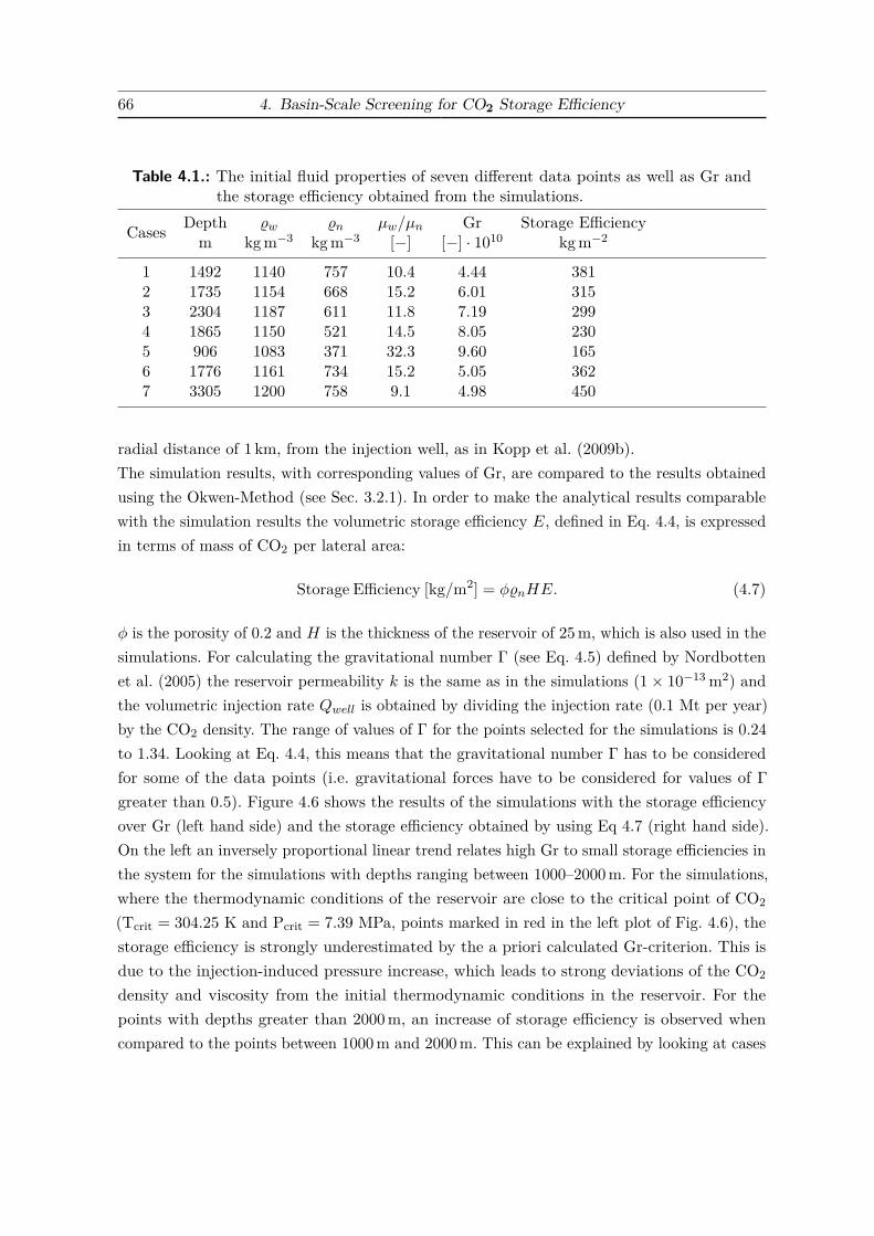
66 4. Basin-Scale Screening for CO2 Storage Efficiency
Table 4.1.: The initial fluid properties of seven different data points as well as Gr andthe storage efficiency obtained from the simulations.
Cases Depth %w %n µw/µn Gr Storage Efficiencym kgm−3 kgm−3 [−] [−] · 1010 kgm−2
1 1492 1140 757 10.4 4.44 3812 1735 1154 668 15.2 6.01 3153 2304 1187 611 11.8 7.19 2994 1865 1150 521 14.5 8.05 2305 906 1083 371 32.3 9.60 1656 1776 1161 734 15.2 5.05 3627 3305 1200 758 9.1 4.98 450
radial distance of 1 km, from the injection well, as in Kopp et al. (2009b).The simulation results, with corresponding values of Gr, are compared to the results obtainedusing the Okwen-Method (see Sec. 3.2.1). In order to make the analytical results comparablewith the simulation results the volumetric storage efficiency E, defined in Eq. 4.4, is expressedin terms of mass of CO2 per lateral area:
Storage Efficiency [kg/m2] = φ%nHE. (4.7)
φ is the porosity of 0.2 and H is the thickness of the reservoir of 25m, which is also used in thesimulations. For calculating the gravitational number Γ (see Eq. 4.5) defined by Nordbottenet al. (2005) the reservoir permeability k is the same as in the simulations (1× 10⁻¹³ m2) andthe volumetric injection rate Qwell is obtained by dividing the injection rate (0.1 Mt per year)by the CO2 density. The range of values of Γ for the points selected for the simulations is 0.24to 1.34. Looking at Eq. 4.4, this means that the gravitational number Γ has to be consideredfor some of the data points (i.e. gravitational forces have to be considered for values of Γgreater than 0.5). Figure 4.6 shows the results of the simulations with the storage efficiencyover Gr (left hand side) and the storage efficiency obtained by using Eq 4.7 (right hand side).On the left an inversely proportional linear trend relates high Gr to small storage efficiencies inthe system for the simulations with depths ranging between 1000–2000m. For the simulations,where the thermodynamic conditions of the reservoir are close to the critical point of CO2
(Tcrit = 304.25 K and Pcrit = 7.39 MPa, points marked in red in the left plot of Fig. 4.6), thestorage efficiency is strongly underestimated by the a priori calculated Gr-criterion. This isdue to the injection-induced pressure increase, which leads to strong deviations of the CO2
density and viscosity from the initial thermodynamic conditions in the reservoir. For thepoints with depths greater than 2000m, an increase of storage efficiency is observed whencompared to the points between 1000m and 2000m. This can be explained by looking at cases
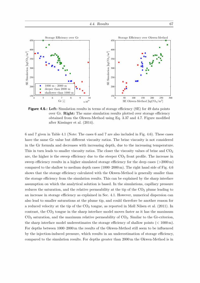
4.4. Results 67
4 5 6 7 8 9 10
x 1010
150
200
250
300
350
400
450
Storage Efficiency over Gr
SESim
ulation[kgCO
2/m
2]
Gr [-]
1000 m - 2000 mdeeper than 2000 m
shallower than 1000 m
0 50 100 150 200 250 300150
200
250
300
350
400
450
Storage Efficiency over Okwen-Method
SESim
ulation[kgCO
2/m
2]
SE Okwen-Method [kgCO2/m2]
Figure 4.6.: Left: Simulation results in terms of storage efficiency (SE) for 49 data pointsover Gr. Right: The same simulation results plotted over storage efficiencyobtained from the Okwen-Method using Eq. 3.37 and 4.7. Figure modifiedafter Kissinger et al. (2014).
6 and 7 given in Table 4.1 (Note: The cases 6 and 7 are also included in Fig. 4.6). These caseshave the same Gr value but different viscosity ratios. The brine viscosity is not consideredin the Gr formula and decreases with increasing depth, due to the increasing temperature.This in turn leads to smaller viscosity ratios. The closer the viscosity values of brine and CO2
are, the higher is the sweep efficiency due to the steeper CO2 front profile. The increase insweep efficiency results in a higher simulated storage efficiency for the deep cases (>2000m)compared to the shallow to medium depth cases (1000–2000m). The right hand side of Fig. 4.6shows that the storage efficiency calculated with the Okwen-Method is generally smaller thanthe storage efficiency from the simulation results. This can be explained by the sharp interfaceassumption on which the analytical solution is based. In the simulations, capillary pressurereduces the saturation, and the relative permeability at the tip of the CO2 plume leading toan increase in storage efficiency as explained in Sec. 4.1. However, numerical dispersion canalso lead to smaller saturations at the plume tip, and could therefore be another reason fora reduced velocity at the tip of the CO2 tongue, as reported in Møll Nilsen et al. (2011). Incontrast, the CO2 tongue in the sharp interface model moves faster as it has the maximumCO2 saturation, and the maximum relative permeability of CO2. Similar to the Gr-criterion,the sharp interface model underestimates the storage efficiency of shallow points (< 1000m).For depths between 1000–2000m the results of the Okwen-Method still seem to be influencedby the injection-induced pressure, which results in an underestimation of storage efficiency,compared to the simulation results. For depths greater than 2000m the Okwen-Method is in
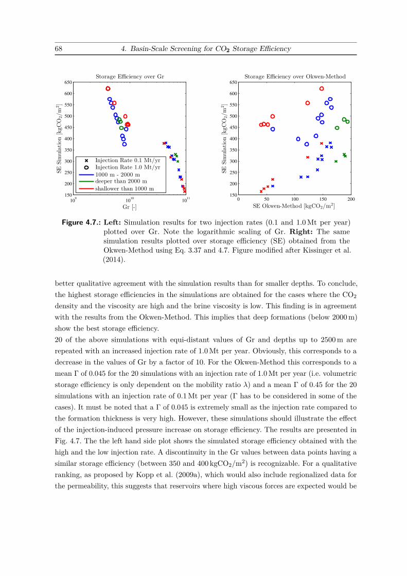
68 4. Basin-Scale Screening for CO2 Storage Efficiency
109
1010
1011
150
200
250
300
350
400
450
500
550
600
650
Gr [-]
SESim
ulation[kgCO
2/m
2]
Storage Efficiency over Gr
Injection Rate 0.1 Mt/yrInjection Rate 1.0 Mt/yr
1000 m - 2000 mdeeper than 2000 m
shallower than 1000 m
0 50 100 150 200150
200
250
300
350
400
450
500
550
600
650
Storage Efficiency over Okwen-Method
SESim
ulation[kgCO
2/m
2]
SE Okwen-Method [kgCO2/m2]
Figure 4.7.: Left: Simulation results for two injection rates (0.1 and 1.0Mt per year)plotted over Gr. Note the logarithmic scaling of Gr. Right: The samesimulation results plotted over storage efficiency (SE) obtained from theOkwen-Method using Eq. 3.37 and 4.7. Figure modified after Kissinger et al.(2014).
better qualitative agreement with the simulation results than for smaller depths. To conclude,the highest storage efficiencies in the simulations are obtained for the cases where the CO2
density and the viscosity are high and the brine viscosity is low. This finding is in agreementwith the results from the Okwen-Method. This implies that deep formations (below 2000m)show the best storage efficiency.20 of the above simulations with equi-distant values of Gr and depths up to 2500m arerepeated with an increased injection rate of 1.0Mt per year. Obviously, this corresponds to adecrease in the values of Gr by a factor of 10. For the Okwen-Method this corresponds to amean Γ of 0.045 for the 20 simulations with an injection rate of 1.0Mt per year (i.e. volumetricstorage efficiency is only dependent on the mobility ratio λ) and a mean Γ of 0.45 for the 20simulations with an injection rate of 0.1Mt per year (Γ has to be considered in some of thecases). It must be noted that a Γ of 0.045 is extremely small as the injection rate compared tothe formation thickness is very high. However, these simulations should illustrate the effectof the injection-induced pressure increase on storage efficiency. The results are presented inFig. 4.7. The the left hand side plot shows the simulated storage efficiency obtained with thehigh and the low injection rate. A discontinuity in the Gr values between data points having asimilar storage efficiency (between 350 and 400 kgCO2/m2) is recognizable. For a qualitativeranking, as proposed by Kopp et al. (2009a), which would also include regionalized data forthe permeability, this suggests that reservoirs where high viscous forces are expected would be
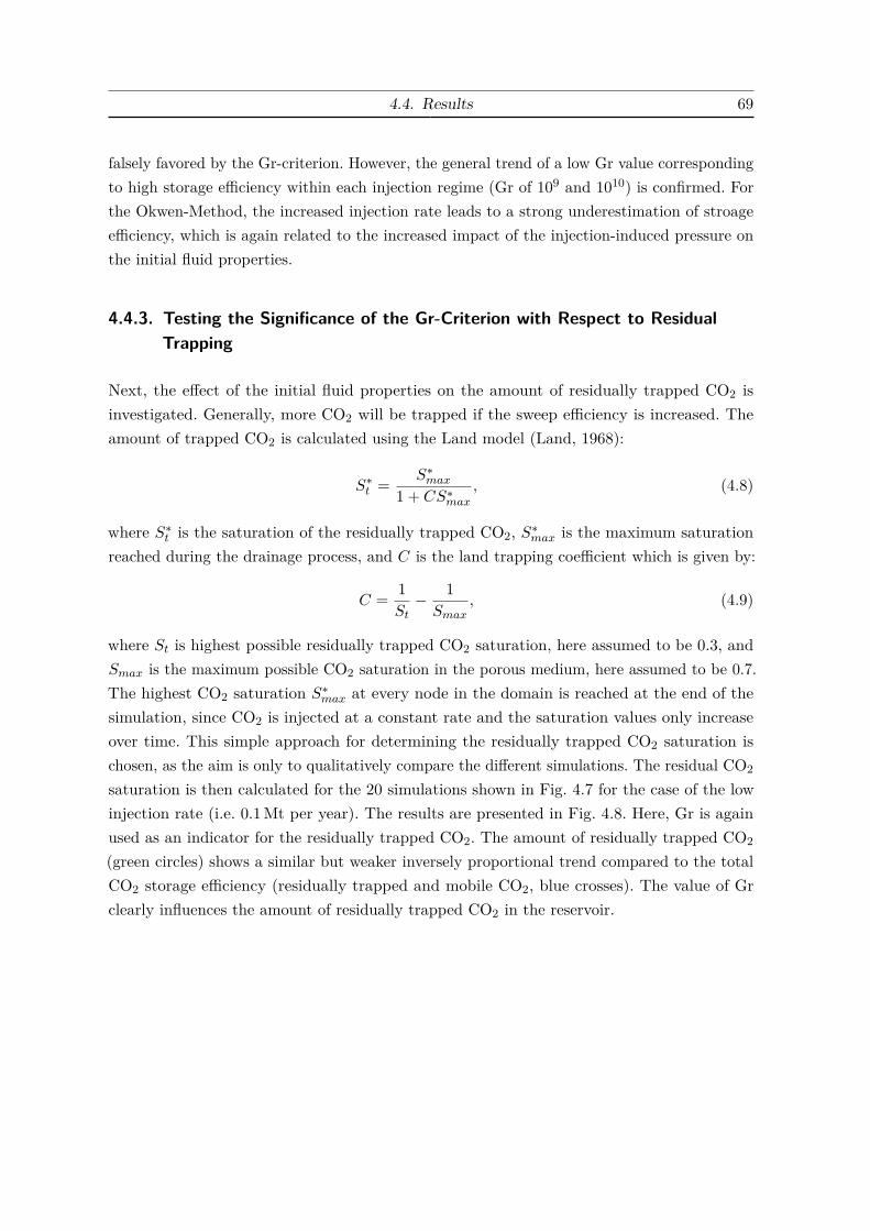
4.4. Results 69
falsely favored by the Gr-criterion. However, the general trend of a low Gr value correspondingto high storage efficiency within each injection regime (Gr of 109 and 1010) is confirmed. Forthe Okwen-Method, the increased injection rate leads to a strong underestimation of stroageefficiency, which is again related to the increased impact of the injection-induced pressure onthe initial fluid properties.
4.4.3. Testing the Significance of the Gr-Criterion with Respect to ResidualTrapping
Next, the effect of the initial fluid properties on the amount of residually trapped CO2 isinvestigated. Generally, more CO2 will be trapped if the sweep efficiency is increased. Theamount of trapped CO2 is calculated using the Land model (Land, 1968):
S∗t = S∗max1 + CS∗max
, (4.8)
where S∗t is the saturation of the residually trapped CO2, S∗max is the maximum saturationreached during the drainage process, and C is the land trapping coefficient which is given by:
C = 1St− 1Smax
, (4.9)
where St is highest possible residually trapped CO2 saturation, here assumed to be 0.3, andSmax is the maximum possible CO2 saturation in the porous medium, here assumed to be 0.7.The highest CO2 saturation S∗max at every node in the domain is reached at the end of thesimulation, since CO2 is injected at a constant rate and the saturation values only increaseover time. This simple approach for determining the residually trapped CO2 saturation ischosen, as the aim is only to qualitatively compare the different simulations. The residual CO2
saturation is then calculated for the 20 simulations shown in Fig. 4.7 for the case of the lowinjection rate (i.e. 0.1Mt per year). The results are presented in Fig. 4.8. Here, Gr is againused as an indicator for the residually trapped CO2. The amount of residually trapped CO2
(green circles) shows a similar but weaker inversely proportional trend compared to the totalCO2 storage efficiency (residually trapped and mobile CO2, blue crosses). The value of Grclearly influences the amount of residually trapped CO2 in the reservoir.
70 4. Basin-Scale Screening for CO2 Storage Efficiency
4 5 6 7 8 9 10
x 1010
0
50
100
150
200
250
300
350
400
Gr [-]
SE[kgCO
2/m
2]
Injection Rate 0.1 Mt per year
Total CO2 (mobile + residually trapped)
CO2 residually trapped in reservoir
Figure 4.8.: Comparison of storage efficiency (SE) and the residually trapped CO2 mass(also given in terms of storage efficiency, i.e. kg/m2). Figure modified af-ter Kissinger et al. (2014).
4.4.4. Testing the Significance of the Gr-Criterion with Respect to Porosity andReservoir Thickness
Permeability, reservoir thickness and porosity are crucial parameters to assess the significanceof reservoir units (Reinhold et al., 2011). However, in this study permeability cannot beconsidered since there is not sufficient data available to reliably account for its basin-widevariability. An analysis of the significance of the Gr-criterion can only be carried out withrespect to the variation of the parameters reservoir thickness and porosity. Three areas ofhigh, medium, and low values of Gr were selected by the project partners of the BGR, wheredata for the reservoir thickness and the porosity are available. More information regarding thesources of these data is given in Kissinger et al. (2014). The locations of these areas are shownin Fig. 4.5. The characteristic parameters of the three areas are listed in Table 4.2.Area 1 (Mean Gr value: 4.85× 10¹⁰) represents regions with a small value of Gr. Accordingto the database, the thickness varies between 6 and 20m. The porosity values range from 0.11to 0.30.Area 2 (Mean Gr value: 5.73× 10¹⁰) is related to regions with medium values of Gr. For thisarea the thickness varies between 5 and 20m, whereas porosity data ranges from 0.06 to 0.25.Area 3 (Mean Gr value: 7.27× 10¹⁰ ) represents regions with the highest Gr values. For thisregion an average thickness of 10m and porosities between 0.04 to 0.08 are reported.In order to deal with the variability of the porosity and thickness data in the three areas,
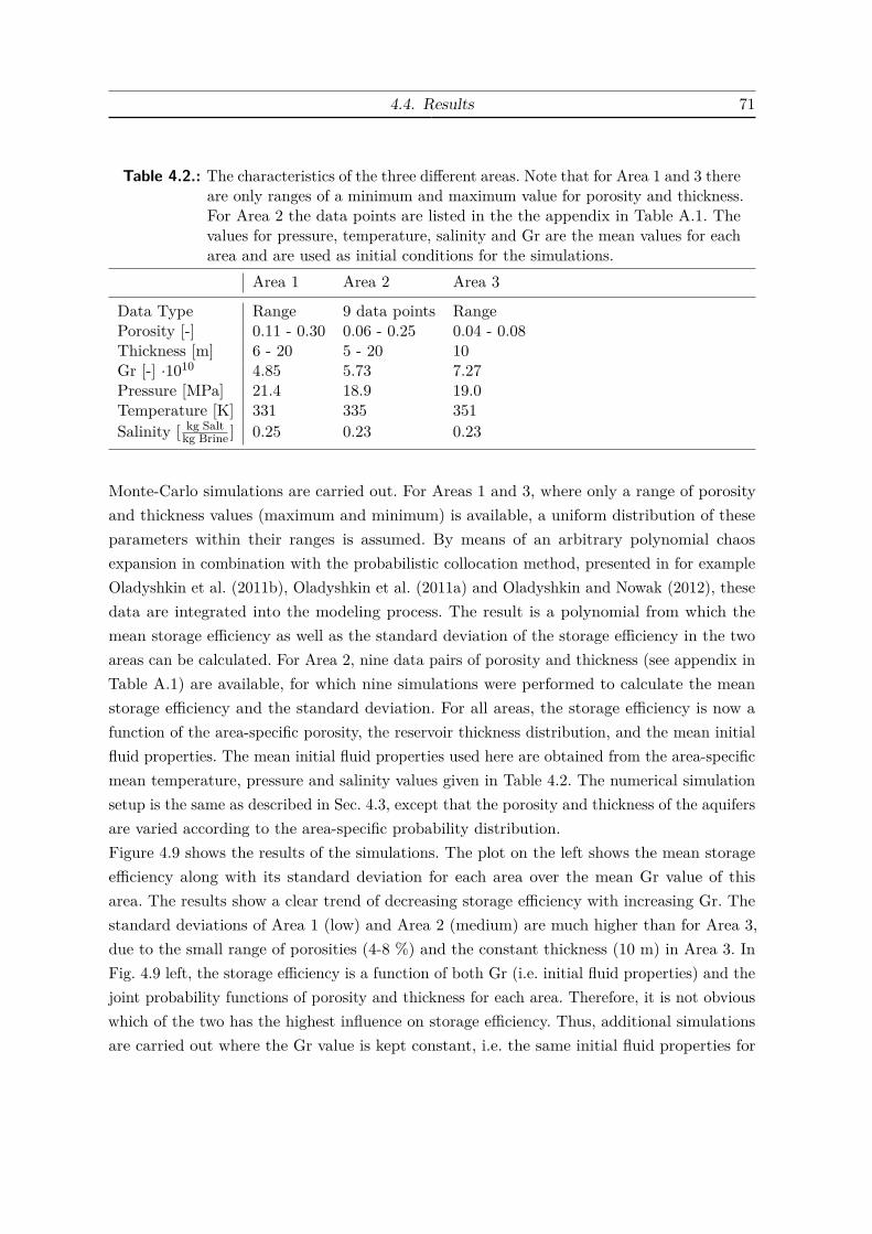
4.4. Results 71
Table 4.2.: The characteristics of the three different areas. Note that for Area 1 and 3 thereare only ranges of a minimum and maximum value for porosity and thickness.For Area 2 the data points are listed in the the appendix in Table A.1. Thevalues for pressure, temperature, salinity and Gr are the mean values for eacharea and are used as initial conditions for the simulations.
Area 1 Area 2 Area 3
Data Type Range 9 data points RangePorosity [-] 0.11 - 0.30 0.06 - 0.25 0.04 - 0.08Thickness [m] 6 - 20 5 - 20 10Gr [-] ·1010 4.85 5.73 7.27Pressure [MPa] 21.4 18.9 19.0Temperature [K] 331 335 351Salinity [ kg Salt
kg Brine ] 0.25 0.23 0.23
Monte-Carlo simulations are carried out. For Areas 1 and 3, where only a range of porosityand thickness values (maximum and minimum) is available, a uniform distribution of theseparameters within their ranges is assumed. By means of an arbitrary polynomial chaosexpansion in combination with the probabilistic collocation method, presented in for exampleOladyshkin et al. (2011b), Oladyshkin et al. (2011a) and Oladyshkin and Nowak (2012), thesedata are integrated into the modeling process. The result is a polynomial from which themean storage efficiency as well as the standard deviation of the storage efficiency in the twoareas can be calculated. For Area 2, nine data pairs of porosity and thickness (see appendix inTable A.1) are available, for which nine simulations were performed to calculate the meanstorage efficiency and the standard deviation. For all areas, the storage efficiency is now afunction of the area-specific porosity, the reservoir thickness distribution, and the mean initialfluid properties. The mean initial fluid properties used here are obtained from the area-specificmean temperature, pressure and salinity values given in Table 4.2. The numerical simulationsetup is the same as described in Sec. 4.3, except that the porosity and thickness of the aquifersare varied according to the area-specific probability distribution.Figure 4.9 shows the results of the simulations. The plot on the left shows the mean storageefficiency along with its standard deviation for each area over the mean Gr value of thisarea. The results show a clear trend of decreasing storage efficiency with increasing Gr. Thestandard deviations of Area 1 (low) and Area 2 (medium) are much higher than for Area 3,due to the small range of porosities (4-8 %) and the constant thickness (10 m) in Area 3. InFig. 4.9 left, the storage efficiency is a function of both Gr (i.e. initial fluid properties) and thejoint probability functions of porosity and thickness for each area. Therefore, it is not obviouswhich of the two has the highest influence on storage efficiency. Thus, additional simulationsare carried out where the Gr value is kept constant, i.e. the same initial fluid properties for
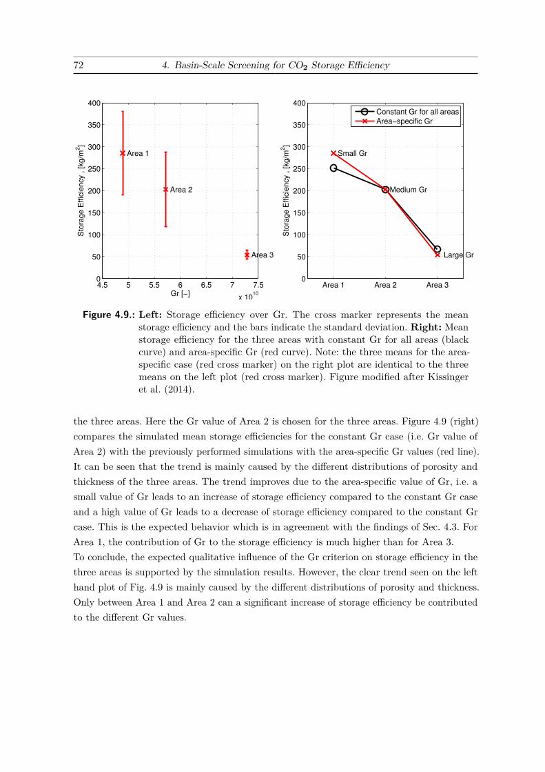
72 4. Basin-Scale Screening for CO2 Storage Efficiency
4.5 5 5.5 6 6.5 7 7.5
x 1010
0
50
100
150
200
250
300
350
400
Sto
rage E
ffic
iency , [kg/m
2]
Gr [−]
Area 3
Area 2
Area 1
Area 1 Area 2 Area 30
50
100
150
200
250
300
350
400
Small Gr
Medium Gr
Large Gr
Sto
rage E
ffic
iency , [kg/m
2]
Constant Gr for all areas
Area−specific Gr
Figure 4.9.: Left: Storage efficiency over Gr. The cross marker represents the meanstorage efficiency and the bars indicate the standard deviation. Right: Meanstorage efficiency for the three areas with constant Gr for all areas (blackcurve) and area-specific Gr (red curve). Note: the three means for the area-specific case (red cross marker) on the right plot are identical to the threemeans on the left plot (red cross marker). Figure modified after Kissingeret al. (2014).
the three areas. Here the Gr value of Area 2 is chosen for the three areas. Figure 4.9 (right)compares the simulated mean storage efficiencies for the constant Gr case (i.e. Gr value ofArea 2) with the previously performed simulations with the area-specific Gr values (red line).It can be seen that the trend is mainly caused by the different distributions of porosity andthickness of the three areas. The trend improves due to the area-specific value of Gr, i.e. asmall value of Gr leads to an increase of storage efficiency compared to the constant Gr caseand a high value of Gr leads to a decrease of storage efficiency compared to the constant Grcase. This is the expected behavior which is in agreement with the findings of Sec. 4.3. ForArea 1, the contribution of Gr to the storage efficiency is much higher than for Area 3.To conclude, the expected qualitative influence of the Gr criterion on storage efficiency in thethree areas is supported by the simulation results. However, the clear trend seen on the lefthand plot of Fig. 4.9 is mainly caused by the different distributions of porosity and thickness.Only between Area 1 and Area 2 can a significant increase of storage efficiency be contributedto the different Gr values.
4.5. Discussion 73
4.5. Discussion
There are different criteria that can be used for a basin-scale site screening for CO2 sequestra-tion. Among others, the Gr-criterion (Kopp et al., 2009a) or the analytical solution by Okwenet al. (2010) can be useful criteria to consider for estimating storage efficiency. Due to aninsufficient regional database of hydrogeological parameters, such as permeability porosity,and reservoir thickness, the input data here are restricted to reservoir depth, temperatureconditions, and salt concentrations. For this study, only the Middle Buntsandstein rock unitis considered. However, the Gr-criterion or the Okwen-Method may also be applied to otherstorage units within the Storage Catalogue of Germany.As the simulations in Sec. 4.4.2 show, the Gr-criterion may be used to distinguish areas withmore or less favorable initial fluid properties. Care should be taken when comparing areas ofsmall to medium depths (1000–2000m) to areas of large depths (>2000m). As the simulationshave shown, the decrease in brine viscosity with depth due to increasing temperature leadsto a smaller viscosity ratio which increases the storage efficiency. This behavior cannot bedescribed with the Gr-criterion. The Okwen-Method, also considers the variation in brineviscosity, and therefore shows a more consistent trend for larger depths. An additional advan-tage of the Okwen-Method is that it can be used to quantify storage efficiency, in contrastto the Gr-criterion which only allows for a qualitative ranking. If, for example, data for theporosity were regionally available, this data could easily be incorporated in the Okwen-Method.The simulations further show, that changes in pressure, caused by the injection, lead to anunderestimation of storage efficiency in areas having conditions close to the critical point ofCO2. But also for the depth range of 1000–2000m, the Okwen-Method seems to underestimatestorgae efficiency, due to these changes in the CO2 fluid properties.For the simulations with a higher injection rate (factor 10 increase), the viscous forces increaseand therefore, the values of Gr decrease by the same factor. However, the storage efficiencydoes not increase as much as would be expected from the Gr-criterion. For a qualitativeranking, which would include regionalized data for the permeability, that may vary over ordersof magnitude, the Gr-criterion may falsely favor regions with a very low permeability (i.e.very high viscous forces) over regions with a higher permeability. This ambiguity has to beconsidered when choosing appropriate methods for a basin-scale screening, also bearing inmind that such methods or criteria should be transparent and comprehensible to stakeholders.Therefore, the use of Gr as a screening criterion should be restricted to ranking regions withmore or less favorable initial fluid properties for CO2 storage. The Okwen-Method clearlyunderestimates the storage efficiency for the cases with an increased injection rate, as it cannotaccount for the effect of the injection-induced pressure increase on the fluid properties of CO2.Considering a case where regionalized data for permeability would be available, low per-

74 4. Basin-Scale Screening for CO2 Storage Efficiency
meabilities could reduce the injectivity, and therefore also the storage efficiency. Thus, anadditional constraint on pressure, which should not exceed the fracturing pressure would berequired. Areas could be excluded by using the method proposed by Mathias et al. (2008,2009), which allows for the determination of the maximum pressure buildup during a CO2
injection. Considering the plume extent which is also used as a constraint in this work (i.e.spill point), the reservoir geometry plays an important role (e.g. dipping or anticlinal) thatmay significantly influence storage efficiency as well (Goater et al., 2013). This discussionmakes it clear that criteria like the Gr-criterion or the Okwen-Method can only be part of alarger set of criteria that have to evaluated.The effect of the Gr-criterion on the amount of residually trapped CO2 described in Sec. 4.4.2is recognizable and confirms the expected increase in residually trapped CO2 for systems withlower Gr values compared to systems with higher Gr values. Hence, a low Gr value is likely tobe beneficial for long term storage safety.The simulations in Sec. 4.4.4 illustrate that changes in storage efficiency, due to variableporosities and reservoir thicknesses, are larger than the changes between a low, a medium, anda high value of Gr. Nevertheless, the influence on storage efficiency caused by different valuesof Gr (i.e. different initial fluid properties) may still be in the same range as the influence ofthe area-specific distributions of porosity and reservoir thickness. It must be noted that thedatabase of porosity and reservoir thickness used here is not very large and that more datawould be necessary to get the complete picture. However, the simulations may still help togain an insight on the effect of the variability of these parameters.
4.6. Conclusion
The main results and findings of this chapter are summarized briefly below:
• The simulations show that the variations of depth, temperature conditions and saltconcentrations, as found in the Middle Buntsandstein rock unit of the North GermanBasin have a noticeable influence on the CO2 and brine densities and viscosities, andthus on storage efficiency.
• Storage efficiency is highest for depths greater than 2000m where the CO2 density andthe viscosity are high and the brine viscosity is low. This result is in agreement with theOkwen-Method and simulations by Kopp et al. (2009b) for deep reservoirs with a smallviscosity ratio (µw/µn).

4.6. Conclusion 75
• The regional Gr distribution for the Middle Buntsandstein rock unit is mainly affectedby the regional variations of the geothermal gradient.
• With some restrictions both Gr and the Okwen-Method can be used as indicators forstorage efficiency.
• The simulations confirm the trend of decreasing Gr values leading to an increasing storageefficiency. Low values of Gr leading to a more compact CO2 plume are in agreementwith findings in Nazarian et al. (2013), where a similar formulation of Gr was used.
• At depths greater than 2000m, the Gr-criterion starts to underestimates storage efficiency,as the effect of a decreasing brine viscosity is not considered. Here, the Okwen-Methodshows a more continuous trend.
• The Gr approach and the Okwen-Method both underestimate the storage efficiencyfor thermodynamic conditions close to or below the critical point of CO2, as the fluidproperties of CO2 are very sensitive to pressure changes caused by the injection.
• Smaller Gr values lead to more residually trapped CO2 in the reservoir, and to morestorage security. This result is in qualitative agreement with the findings of Taku Ideet al. (2007).
• Comparing the contribution of the initial fluid properties on storage efficiency to thecontribution of the parameters porosity and reservoir thickness, shows that the porosityand the reservoir thickness are more important. However, the contribution ot the initialfluid properties can still be in the same range as that of the other two parameters.

5. Large-Scale Investigation of BrineDisplacement1
In this chapter, the focus lies on the effects of large-scale brine migration due to CO2 injectionin a realistic (but not real) geological structure in the North German Basin. The latter isthe most relevant region regarding CO2 storage capacity in Germany (Knopf et al., 2010).The geological model comprises layers from the Lower Buntsandstein up to potential drinkingwater horizons in shallow, freshwater aquifers along with characteristic geological features ofthe North German Basin. In contrast to earlier work for example by Kempka et al. (2013), themodel presented here fully couples flow in shallow aquifers with deep saline aquifers consideringvariable-density flow. As uncertainty is inherent to hydrogeological problems, a classificationof different types of uncertainty is made in Sec. 5.1, which helps in categorizing the resultspresented later. The data available for the geological model and the numerical model setup arepresented in Sec. 5.2 and 5.3, respectively. The reliability of the numerical model is then testedfor (i) large scale pressure propagation due to injection with the Zeidouni-Method (Sec. 5.4.1)and (ii) variable-density flow using experimental data from the popular saltpool benchmark(Sec. 5.4.2). The results section has the following aims:
• Definition of target variables, suitable for the analysis of brine displacement (Sec. 5.5.1).
• Analysis of different scenarios in order to identity relevant components of the geologicalmodel controlling brine displacement (Sec. 5.5.2).
• Comparative analysis of model simplifications, in order to develop an understandingwhat assumptions in the model may be relevant and when, i.e. to design the optimalmodel with respect to required accuracy, computational costs, data availability and theuncertainty in these data (Sec. 5.5.3).
1Large parts of this chapter will be published in Kissinger et al. (2017).

78 5. Large-Scale Investigation of Brine Displacement
5.1. Uncertainty Categorization and Brine Displacement
Every model result is inherently subject to uncertainty, mainly from input data and frommodel assumptions. The type of uncertainty can be categorized along with a qualitative orquantitative estimation of the model uncertainty. Communicating uncertainty in simulationresults is a crucial aspect for decision making. The approach by Walker et al. (2003), for theclassification of uncertainties, is followed here, similarly to Walter et al. (2012), who haveadopted this approach in the context of risk estimation for CO2 storage. Walker et al. (2003)categorize the uncertainties into different levels on a scale (see Fig. 5.1) where determinism(a hypothetical state where everything is known) is on the far left end of the scale. The firstlevel of uncertainty is statistical uncertainty which accounts for all model parameters thatcan be described by statistical terms, for example, a probability density function (PDF).In the hydrogeological context this can be, for example, a probability density function of
Figure 5.1.: Levels of uncertainty after Walker et al. (2003), modified by Walter et al.(2012).
permeability or porosity. The second level is defined as scenario uncertainty and includesparameters which cannot readily be described by statistical terms. This could be the existenceof a certain geological feature, like the presence of a permeable fault zone at a certain location,or the type of boundary condition chosen on the lateral boundaries, etc. The next level isrecognized ignorance which is defined by Walker et al. (2003) as fundamental uncertaintiesabout mechanisms and functionalities. Recognized ignorance is any uncertainty caused byneglecting certain physical processes within the model concept. It will also be referred to asmodel uncertainty in this work. A model is always an abstraction of reality, as complex asnecessary and as simple as possible. In contrast to the last category, total ignorance, whichstands for all uncertainties that have simply not been recognized yet, model uncertainty canbe reduced by comparing models of different conceptual complexity. The analysis presentedbelow will focus on scenario uncertainty, and model uncertainty (i.e. recognized ignorance).
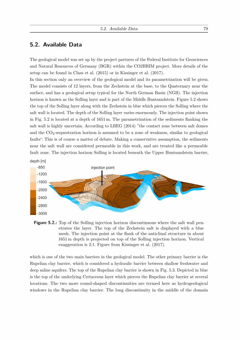
5.2. Available Data 79
5.2. Available Data
The geological model was set up by the project partners of the Federal Institute for Geosciencesand Natural Resources of Germany (BGR) within the CO2BRIM project. More details of thesetup can be found in Class et al. (2015) or in Kissinger et al. (2017).In this section only an overview of the geological model and its parametrization will be given.The model consists of 12 layers, from the Zechstein at the base, to the Quaternary near thesurface, and has a geological setup typical for the North German Basin (NGB). The injectionhorizon is known as the Solling layer and is part of the Middle Buntsandstein. Figure 5.2 showsthe top of the Solling layer along with the Zechstein in blue which pierces the Solling where thesalt wall is located. The depth of the Solling layer varies enormously. The injection point shownin Fig. 5.2 is located at a depth of 1651m. The parametrization of the sediments flanking thesalt wall is highly uncertain. According to LBEG (2014) ”the contact zone between salt domesand the CO2-sequestration horizon is assumed to be a zone of weakness, similar to geologicalfaults“. This is of course a matter of debate. Making a conservative assumption, the sedimentsnear the salt wall are considered permeable in this work, and are treated like a permeablefault zone. The injection horizon Solling is located beneath the Upper Buntsandstein barrier,
Figure 5.2.: Top of the Solling injection horizon discontinuous where the salt wall pen-etrates the layer. The top of the Zechstein salt is displayed with a bluemesh. The injection point at the flank of the anticlinal structure in about1651m depth is projected on top of the Solling injection horizon. Verticalexaggeration is 2:1. Figure from Kissinger et al. (2017).
which is one of the two main barriers in the geological model. The other primary barrier is theRupelian clay barrier, which is considered a hydraulic barrier between shallow freshwater anddeep saline aquifers. The top of the Rupelian clay barrier is shown in Fig. 5.3. Depicted in blueis the top of the underlying Cretaceous layer which pierces the Rupelian clay barrier at severallocations. The two more round-shaped discontinuities are termed here as hydrogeologicalwindows in the Rupelian clay barrier. The long discontinuity in the middle of the domain

80 5. Large-Scale Investigation of Brine Displacement
is caused by the salt wall lifting the Cretaceous layer. These three discontinuities play animportant role in the exchange between saline water and freshwater. In the context of CO2
storage, they can be considered potential pathways for saltwater. The Upper Buntsandsteinbarrier is discontinuous at the locations where is is penetrated by the salt wall, similar tothe injection horizon Solling shown in Fig. 5.2. The top of the geological model consists of
Figure 5.3.: Top of the Rupelian clay barrier with discontinuities where Cretaceoussediments penetrate the Rupelian clay barrier. The top of the Cretaceous isdisplayed as blue mesh. Vertical exaggeration is 2:1. Figure from Kissingeret al. (2017).
groundwater isolines from an upper freshwater aquifer. In order to simulate the groundwaterflow in the shallow aquifers data of the main rivers derived from the associated catchment areaare used, see Fig. 5.4. Both datasets (groundwater isolines and data on rivers) were preparedto be used as upper boundary conditions on top of the model (data provided by LUGV (2012);LUGV (2014)).The different layers and the grid are shown in Fig. 5.5. The grid consists of hexahedralelements with a constant horizontal discretization length of 300m× 300m. The verticalresolution depends on the thickness of each layer resolved in the model, and varies between 10and 300m. The smallest vertical resolution, 10m, is found within the injection horizon Solling.Each layer is assumed to be homogeneous, i.e. having a single permeability and porosity valueassigned to it. The parametrization of the layers is given in Table 5.1. Data for lithologicalcomposition and the corresponding hydrogeological parameters are derived from regionalliterature data and numerical simulation studies (Larue, 2010; Reutter, 2011; Schäfer et al.,2011; Noack et al., 2013). Since the Zechstein layer is impermeable, it is not included in thenumerical model, except for the parts where the salt wall penetrates the above layers. As canbe seen in Table 5.1, the Quaternary unit is split into two parts. Compared to the bottomsection of this Quaternary unit (Quaternary 2), the top section (Quaternary 1) has a higher

5.2. Available Data 81
4
8
12
16∆ Z [m]
0
Figure 5.4.: Top view on the groundwater table. The rivers are highlighted in blue. Theelevation values are normalized to the minimum elevation of the groundwatertable. Figure from Kissinger et al. (2017).
Figure 5.5.: Perspective view on the 3D geological model with zoom in on the anticlinalstructure showing the mesh of the 3D volume model. Vertical exaggeration2:1. Here Quaternary 1 and 2 are combined in the Quaternary layer. Figurefrom Kissinger et al. (2017).
permeability. This is the result of a stationary calibration performed in order to obtain a
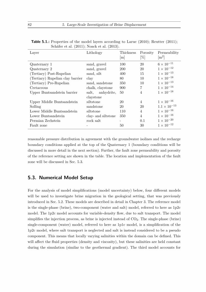
82 5. Large-Scale Investigation of Brine Displacement
Table 5.1.: Properties of the model layers according to Larue (2010); Reutter (2011);Schäfer et al. (2011); Noack et al. (2013).
Layer Lithology Thickness Porosity Permeability[m] [%] [m2]
Quaternary 1 sand, gravel 100 20 6× 10⁻¹¹
Quaternary 2 sand, gravel 200 20 1× 10⁻¹²
(Tertiary) Post-Rupelian sand, silt 400 15 1× 10⁻¹³
(Tertiary) Rupelian clay barrier clay 80 10 1× 10⁻¹⁸
(Tertiary) Pre-Rupelian sand, sandstone 350 10 1× 10⁻¹³
Cretaceous chalk, claystone 900 7 1× 10⁻¹⁴
Upper Buntsandstein barrier salt, anhydrite,claystone
50 4 1× 10⁻¹⁸
Upper Middle Buntsandstein siltstone 20 4 1× 10⁻¹⁶
Solling sandstone 20 20 1.1× 10⁻¹³
Lower Middle Buntsandstein siltstone 110 4 1× 10⁻¹⁶
Lower Buntsandstein clay- and siltstone 350 4 1× 10⁻¹⁶
Permian Zechstein rock salt - 0.1 1× 10⁻²⁰
Fault zone - 50 30 1× 10⁻¹²
reasonable pressure distribution in agreement with the groundwater isolines and the rechargeboundary conditions applied at the top of the Quaternary 1 (boundary conditions will bediscussed in more detail in the next section). Further, the fault zone permeability and porosityof the reference setting are shown in the table. The location and implementation of the faultzone will be discussed in Sec. 5.3.
5.3. Numerical Model Setup
For the analysis of model simplifications (model uncertainty) below, four different modelswill be used to investigate brine migration in the geological setting, that was previouslyintroduced in Sec. 5.2. These models are described in detail in Chapter 3. The reference modelis the single-phase (brine), two-component (water and salt) model, referred to here as 1p2cmodel. The 1p2c model accounts for variable-density flow, due to salt transport. The modelsimplifies the injection process, as brine is injected instead of CO2. The single-phase (brine)single-component (water) model, referred to here as 1p1c model, is a simplification of the1p2c model, where salt transport is neglected and salt is instead considered to be a pseudocomponent. This means that locally varying salinities within the domain can be defined. Thiswill affect the fluid properties (density and viscosity), but these salinities are held constantduring the simulation (similar to the geothermal gradient). The third model accounts for
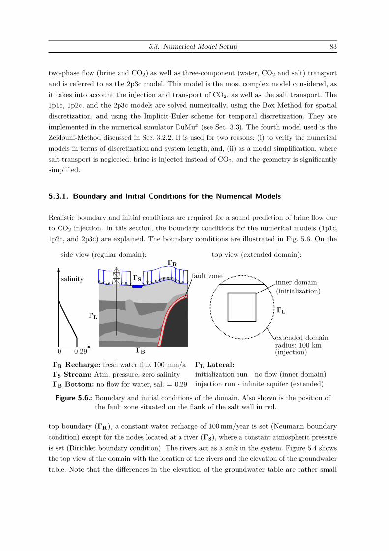
5.3. Numerical Model Setup 83
two-phase flow (brine and CO2) as well as three-component (water, CO2 and salt) transportand is referred to as the 2p3c model. This model is the most complex model considered, asit takes into account the injection and transport of CO2, as well as the salt transport. The1p1c, 1p2c, and the 2p3c models are solved numerically, using the Box-Method for spatialdiscretization, and using the Implicit-Euler scheme for temporal discretization. They areimplemented in the numerical simulator DuMux (see Sec. 3.3). The fourth model used is theZeidouni-Method discussed in Sec. 3.2.2. It is used for two reasons: (i) to verify the numericalmodels in terms of discretization and system length, and, (ii) as a model simplification, wheresalt transport is neglected, brine is injected instead of CO2, and the geometry is significantlysimplified.
5.3.1. Boundary and Initial Conditions for the Numerical Models
Realistic boundary and initial conditions are required for a sound prediction of brine flow dueto CO2 injection. In this section, the boundary conditions for the numerical models (1p1c,1p2c, and 2p3c) are explained. The boundary conditions are illustrated in Fig. 5.6. On the
ΓB
ΓR
ΓS
ΓL
ΓR Recharge: fresh water flux 100 mm/aΓS Stream: Atm. pressure, zero salinity
ΓL Lateral:
ΓB Bottom: no flow for water, sal. = 0.29initialization run - no flow (inner domain)injection run - infinite aquifer (extended)
salinity
0.290
ΓL
extended domain
inner domain
side view (regular domain): top view (extended domain):
(initialization)
(injection)
fault zone
radius: 100 km
Figure 5.6.: Boundary and initial conditions of the domain. Also shown is the position ofthe fault zone situated on the flank of the salt wall in red.
top boundary (ΓR), a constant water recharge of 100mm/year is set (Neumann boundarycondition) except for the nodes located at a river (ΓS), where a constant atmospheric pressureis set (Dirichlet boundary condition). The rivers act as a sink in the system. Figure 5.4 showsthe top view of the domain with the location of the rivers and the elevation of the groundwatertable. Note that the differences in the elevation of the groundwater table are rather small
84 5. Large-Scale Investigation of Brine Displacement
(17 m). It is assumed that full hydraulic contact exists between the rivers and the groundwater.Four episodes are distinguished in the numerical simulations:
1. Pre-initialization episode (1 s)
2. Initialization episode (300 000 years)
3. Injection episode (50 years)
4. Post-injection episode (50 years)
The first two episodes are required to establish a quasi-stationary base flow. The pre-initialization episode is needed to determine the pressure field, which is dependent on thegeothermal gradient, the recharge boundary conditions, and the initial salt distribution, pre-scribed for this episode as a pseudo component. This means that only the pressure is variablein the pre-initialization run. A stationary pressure field can be established with a single timestep. This is achieved by reducing the value of the storage term at every node by several ordersof magnitude via a reduction of the porosities. The initial salt distribution below the RupelianClay Barrier is assumed to follow a linear increase of salinity with depth, with a maximumsalinity of 0.29 kg−Salt/kg−Brine, see Fig. 5.6 (left).The initialization episode (second episode) is required to obtain a quasi-stationary salt dis-tribution. The porosities are set again to their normal values and salt transport is included.The pressure field determined from the pre-initialization episode is used as an initial conditionfor the pressure. Salt may enter the system for the 2p3c and the 1p2c models at the bottomboundary, where a fixed maximum salinity of 0.29 is set. The salt wall acts as another sourceof salt for the 1p2c and the 2p3c models with a fixed maximum salinity of 0.29 assigned toit. However, the maximum salinity is not assigned to the nodes in the fault zone, which islocated at the interface between the salt wall and the surrounding layers. At the fault zone,the salinity is allowed to change. Given the initial salt distribution (linear salt gradient) anon-linear system (variable-density flow) is then solved forward in time. A theoretical steadystate, which would be possible given the boundary and initial conditions is not reached as thesimulations are terminated after a certain time (300 000 years for the cases considered here).The 1p1c model only requires the pre-initialization run, as this model neglects salt transportand treats the salt component as a pseudo component. Both initialization episodes considerthe lateral boundaries to be closed.After the initialization episode, the pressure and the salt distribution are quasi-stationary onthe time scale of the injection and post-injection episodes (100 years). This means that duringthis period, without injection, no recognizable changes in the concentration field occur. Theresults from the initialization episode (i.e. pressure and salinity distribution) serve as an initialcondition for the injection episode. To allow pressure propagation beyond the inner domain

5.4. Numerical Model Reliability 85
during the injection episode, the domain is extended laterally. For this, the grid extensiondescribed in Sec. 3.3.6 is applied for the layers with a permeability greater than 1× 10⁻¹⁵ m2
beneath the Rupelian clay barrier (i.e. Pre-Rupelian, Cretaceous and Solling layers). The gridextension is also illustrated on the right hand side of Fig. 5.6. The layers are extended to adistance of 100 km from the center of gravity of the inner domain. All other lateral boundariesremain closed. As will be shown in Sec. 5.4 this distance is sufficient to make the boundariesof the inner domain act as infinite aquifers.
5.3.2. Fault Zone Representation Using a Discrete-Fracture Model
In the geological model, a fault zone with a width of 50m is considered near the salt wall.Since the horizontal discretization length of the numerical models is about 300m, representingthe geometry of the fault zone accurately would require a grid refinement over large areas. Thiswould substantially increase the computational costs. In order to avoid the grid refinement,the fault zone is implemented with a discrete fracture approach, by defining the fault zone as asingle large fracture, as described in Sec. 3.3.5. A fracture can be described by three parameters:fracture width, fracture permeability, and fracture porosity. Additionally, in Sec. 3.3.5 thematrix and fracture weighting factors Wm and Wf are introduced. Setting Wm to zero, andWf to one, leads to faster transport velocities, as the storage volume on the fracture nodes isreduced. The effect of this assumption is investigated in Sec. 5.5. In the reference case, Wm isset to zero, i.e. decreasing the retention time of the salt component within the fault zone. Theposition of the fault zone is illustrated in the schematic shown in Fig. 5.6 and in Fig. 5.12,marked in red.
5.4. Numerical Model Reliability
To make sure that the 1p2c reference model, is adequate for the problem setting, differentfunctionalities of the 1p2c model are tested in this section using the Zeidouni-Method forlarge-scale pressure evolution, and the experimental results of the saltpool benchmark forvariable-density flow.
5.4.1. Large-Scale Pressure Propagation During Injection
The driving force for brine migration during the injection period is the displacement of brinecaused by the injected fluid. To adequately capture the far-field pressure buildup and brineleakage through the fault zone, the Zeidouni-Method is used. With this method, a reference
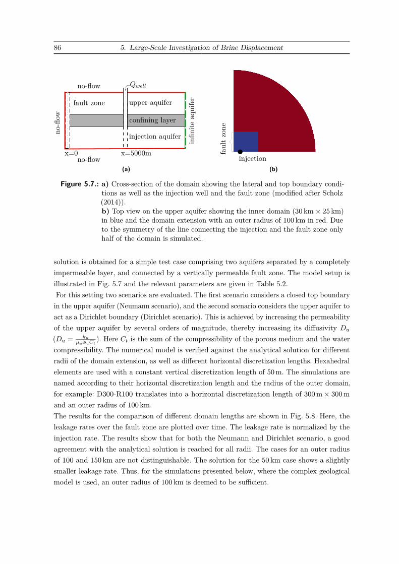
86 5. Large-Scale Investigation of Brine Displacement
fault zone
infin
iteaq
uifer
no-flow
no-flow
no-flow Qwell
x=0 x=5000m
upper aquifer
injection aquifer
confining layer
(a)
faultzone
injection(b)
Figure 5.7.: a) Cross-section of the domain showing the lateral and top boundary condi-tions as well as the injection well and the fault zone (modified after Scholz(2014)).b) Top view on the upper aquifer showing the inner domain (30 km× 25 km)in blue and the domain extension with an outer radius of 100 km in red. Dueto the symmetry of the line connecting the injection and the fault zone onlyhalf of the domain is simulated.
solution is obtained for a simple test case comprising two aquifers separated by a completelyimpermeable layer, and connected by a vertically permeable fault zone. The model setup isillustrated in Fig. 5.7 and the relevant parameters are given in Table 5.2.For this setting two scenarios are evaluated. The first scenario considers a closed top boundaryin the upper aquifer (Neumann scenario), and the second scenario considers the upper aquifer toact as a Dirichlet boundary (Dirichlet scenario). This is achieved by increasing the permeabilityof the upper aquifer by several orders of magnitude, thereby increasing its diffusivity Du
(Du = kuµuφuCt
). Here Ct is the sum of the compressibility of the porous medium and the watercompressibility. The numerical model is verified against the analytical solution for differentradii of the domain extension, as well as different horizontal discretization lengths. Hexahedralelements are used with a constant vertical discretization length of 50m. The simulations arenamed according to their horizontal discretization length and the radius of the outer domain,for example: D300-R100 translates into a horizontal discretization length of 300m× 300mand an outer radius of 100 km.The results for the comparison of different domain lengths are shown in Fig. 5.8. Here, theleakage rates over the fault zone are plotted over time. The leakage rate is normalized by theinjection rate. The results show that for both the Neumann and Dirichlet scenario, a goodagreement with the analytical solution is reached for all radii. The cases for an outer radiusof 100 and 150 km are not distinguishable. The solution for the 50 km case shows a slightlysmaller leakage rate. Thus, for the simulations presented below, where the complex geologicalmodel is used, an outer radius of 100 km is deemed to be sufficient.
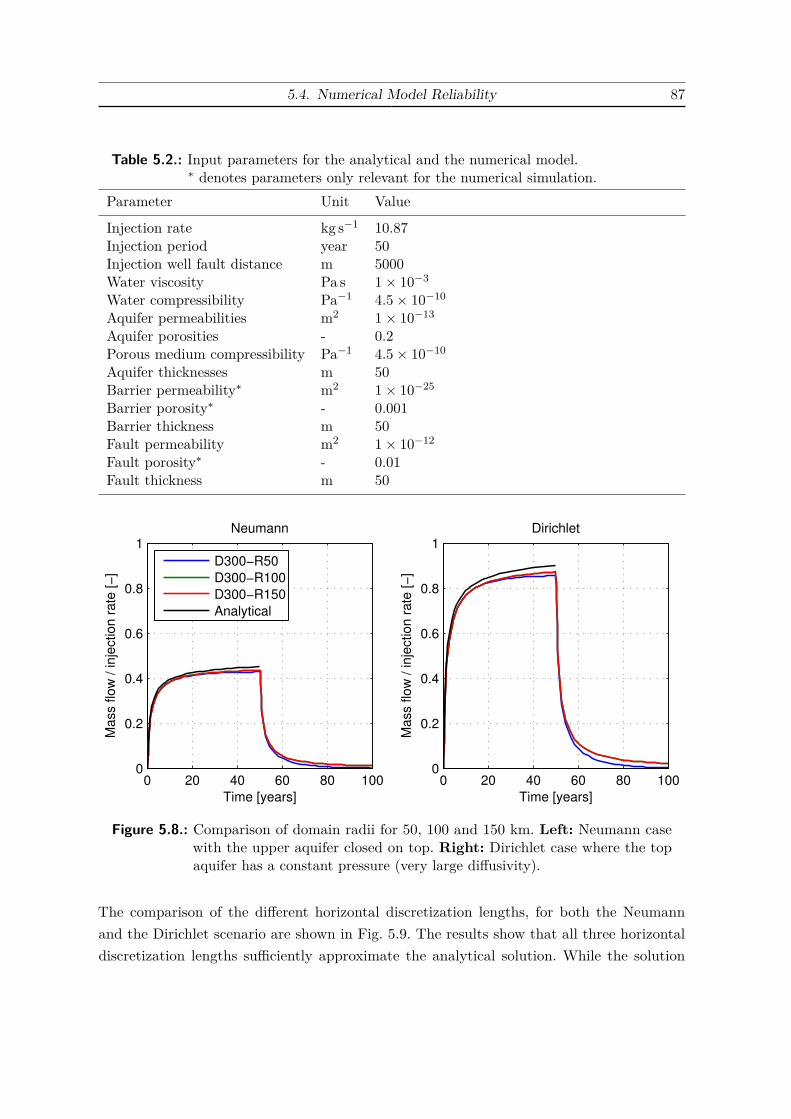
5.4. Numerical Model Reliability 87
Table 5.2.: Input parameters for the analytical and the numerical model.∗ denotes parameters only relevant for the numerical simulation.
Parameter Unit Value
Injection rate kg s−1 10.87Injection period year 50Injection well fault distance m 5000Water viscosity Pa s 1× 10⁻³
Water compressibility Pa−1 4.5× 10⁻¹⁰
Aquifer permeabilities m2 1× 10⁻¹³
Aquifer porosities - 0.2Porous medium compressibility Pa−1 4.5× 10⁻¹⁰
Aquifer thicknesses m 50Barrier permeability∗ m2 1× 10⁻²⁵
Barrier porosity∗ - 0.001Barrier thickness m 50Fault permeability m2 1× 10⁻¹²
Fault porosity∗ - 0.01Fault thickness m 50
0 20 40 60 80 1000
0.2
0.4
0.6
0.8
1Neumann
Time [years]
Mass flo
w / inje
ction r
ate
[−
]
D300−R50
D300−R100
D300−R150
Analytical
0 20 40 60 80 1000
0.2
0.4
0.6
0.8
1Dirichlet
Mass flo
w / inje
ction r
ate
[−
]
Time [years]
Figure 5.8.: Comparison of domain radii for 50, 100 and 150 km. Left: Neumann casewith the upper aquifer closed on top. Right: Dirichlet case where the topaquifer has a constant pressure (very large diffusivity).
The comparison of the different horizontal discretization lengths, for both the Neumannand the Dirichlet scenario are shown in Fig. 5.9. The results show that all three horizontaldiscretization lengths sufficiently approximate the analytical solution. While the solution
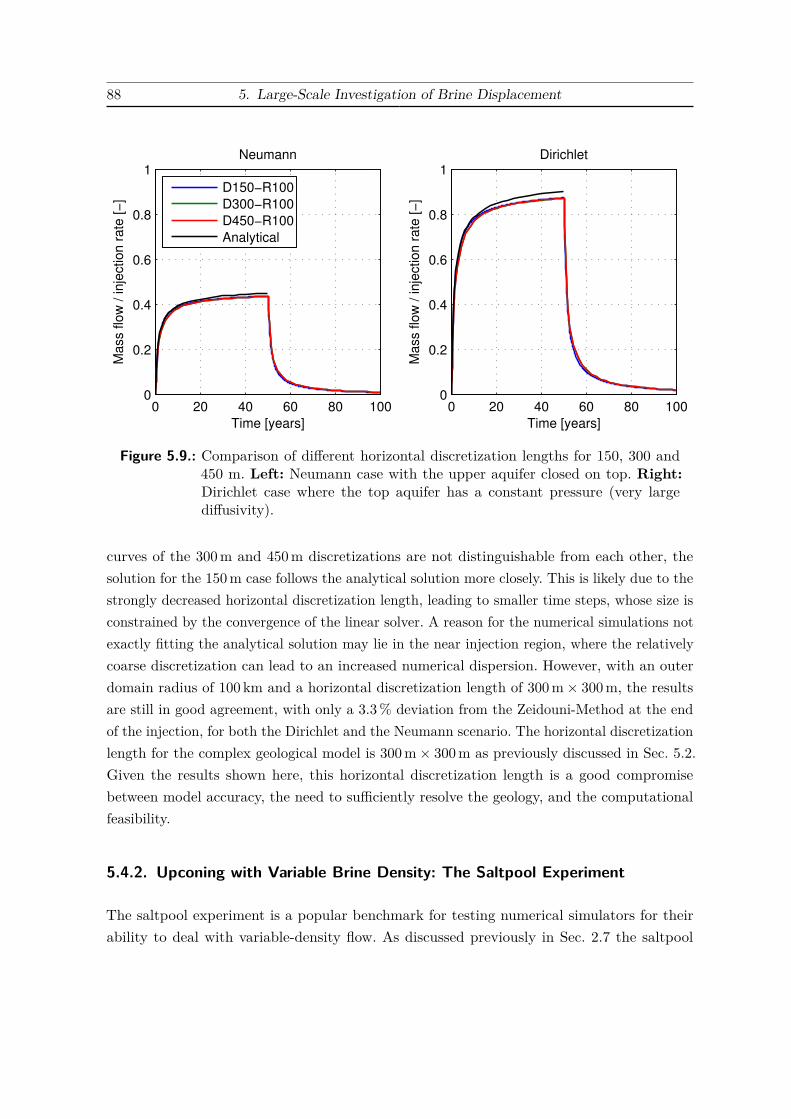
88 5. Large-Scale Investigation of Brine Displacement
0 20 40 60 80 1000
0.2
0.4
0.6
0.8
1Neumann
Time [years]
Mass flo
w / inje
ction r
ate
[−
]
D150−R100
D300−R100
D450−R100
Analytical
0 20 40 60 80 1000
0.2
0.4
0.6
0.8
1Dirichlet
Mass flo
w / inje
ction r
ate
[−
]Time [years]
Figure 5.9.: Comparison of different horizontal discretization lengths for 150, 300 and450 m. Left: Neumann case with the upper aquifer closed on top. Right:Dirichlet case where the top aquifer has a constant pressure (very largediffusivity).
curves of the 300m and 450m discretizations are not distinguishable from each other, thesolution for the 150m case follows the analytical solution more closely. This is likely due to thestrongly decreased horizontal discretization length, leading to smaller time steps, whose size isconstrained by the convergence of the linear solver. A reason for the numerical simulations notexactly fitting the analytical solution may lie in the near injection region, where the relativelycoarse discretization can lead to an increased numerical dispersion. However, with an outerdomain radius of 100 km and a horizontal discretization length of 300m× 300m, the resultsare still in good agreement, with only a 3.3% deviation from the Zeidouni-Method at the endof the injection, for both the Dirichlet and the Neumann scenario. The horizontal discretizationlength for the complex geological model is 300m× 300m as previously discussed in Sec. 5.2.Given the results shown here, this horizontal discretization length is a good compromisebetween model accuracy, the need to sufficiently resolve the geology, and the computationalfeasibility.
5.4.2. Upconing with Variable Brine Density: The Saltpool Experiment
The saltpool experiment is a popular benchmark for testing numerical simulators for theirability to deal with variable-density flow. As discussed previously in Sec. 2.7 the saltpool
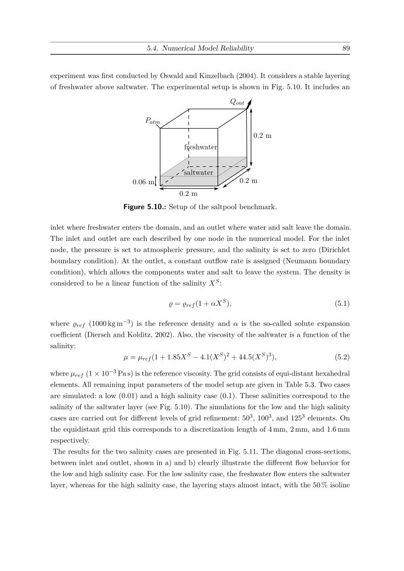
5.4. Numerical Model Reliability 89
experiment was first conducted by Oswald and Kinzelbach (2004). It considers a stable layeringof freshwater above saltwater. The experimental setup is shown in Fig. 5.10. It includes an
0.2 m0.2 m
0.2 m
0.06 m
Qout
Patm
saltwater
freshwater
Figure 5.10.: Setup of the saltpool benchmark.
inlet where freshwater enters the domain, and an outlet where water and salt leave the domain.The inlet and outlet are each described by one node in the numerical model. For the inletnode, the pressure is set to atmospheric pressure, and the salinity is set to zero (Dirichletboundary condition). At the outlet, a constant outflow rate is assigned (Neumann boundarycondition), which allows the components water and salt to leave the system. The density isconsidered to be a linear function of the salinity XS :
% = %ref (1 + αXS), (5.1)
where %ref (1000 kgm−3) is the reference density and α is the so-called solute expansioncoefficient (Diersch and Kolditz, 2002). Also, the viscosity of the saltwater is a function of thesalinity:
µ = µref (1 + 1.85XS − 4.1(XS)2 + 44.5(XS)3), (5.2)
where µref (1× 10⁻³ Pa s) is the reference viscosity. The grid consists of equi-distant hexahedralelements. All remaining input parameters of the model setup are given in Table 5.3. Two casesare simulated: a low (0.01) and a high salinity case (0.1). These salinities correspond to thesalinity of the saltwater layer (see Fig. 5.10). The simulations for the low and the high salinitycases are carried out for different levels of grid refinement: 503, 1003, and 1253 elements. Onthe equidistant grid this corresponds to a discretization length of 4mm, 2mm, and 1.6mmrespectively.The results for the two salinity cases are presented in Fig. 5.11. The diagonal cross-sections,between inlet and outlet, shown in a) and b) clearly illustrate the different flow behavior forthe low and high salinity case. For the low salinity case, the freshwater flow enters the saltwaterlayer, whereas for the high salinity case, the layering stays almost intact, with the 50% isoline

90 5. Large-Scale Investigation of Brine Displacement
Table 5.3.: Input parameters for the saltpool benchmark as given in Oswald and Kinzel-bach (2004).
Parameter Unit Value
Extraction rate (low case) m3 s−1 1.89× 10⁻⁶
Extraction rate (high case) m3 s−1 1.83× 10⁻⁶
Extraction period s 9000Water viscosity Pa s see Eq. 5.2Solute expansion coefficient α (low case) - 0.76Solute expansion coefficient α (high case) - 0.735Permeability m2 9.77× 10⁻¹⁰
Porosity - 0.372Longitudinal dispersion m 1.2× 10⁻³
Transversal dispersion m 1.2× 10⁻⁴
Initial salt layer height m 0.06Initial salt layer salinity (low case) - 0.01Initial salt layer salinity (high case) - 0.1
being horizontal. The main target variable considered in this case is the salinity at the outlet.Figure 5.11 c) and d) show the salinity over time for the low and high salinity case comparedto the experimental results. For both cases, the qualitative behavior of the evolution of thesalinity over time is in good agreement with the experimental results. Different gird resolutionsare compared, and it can be seen that for 1003 and 1253 elements the results are almost gridconvergent for both salinity cases. However, the quantitative agreement, especially for thehigh salinity case, is not satisfactory. Simulated results for the saltpool benchmark can befound in several publications (Bastian et al., 2001; Diersch and Kolditz, 2002; Johannsen et al.,2002; Oswald and Kinzelbach, 2004). Simulations carried out by Bastian et al. (2001) with theoriginal values from Oswald and Kinzelbach (2004), also used here (see Table 5.3), indicate anoverestimation for both the high and the low salinity case. This is especially true for the highsalinity case, as the salinity at the outlet observed by Bastian et al. (2001) with these values ishigher by a factor of almost two. Simulated results for the high salinity case shown in Oswaldand Kinzelbach (2004) cannot even reproduce the experimental results qualitatively, with thesalinity at the outlet continuously increasing over time. To obtain a good agreement, Johannsenet al. (2002) had to fit the values for transversal dispersion (αt), permeability, and porosity,through inverse modeling. This explains the strong deviations observed here too. Additionally,Johannsen et al. (2002), Bastian et al. (2001), and Diersch and Kolditz (2002) stress theimportance of using a consistent velocity approximation as proposed by Knabner et al. (1998),which is not implemented in DuMux. A consistent velocity approximation will mainly decreasethe velocity dependent dispersion (see Sec. 2.6.3), due to erroneous fluxes arising from linearlyapproximating the pressure between two nodes, which in the case of variable-density flow is
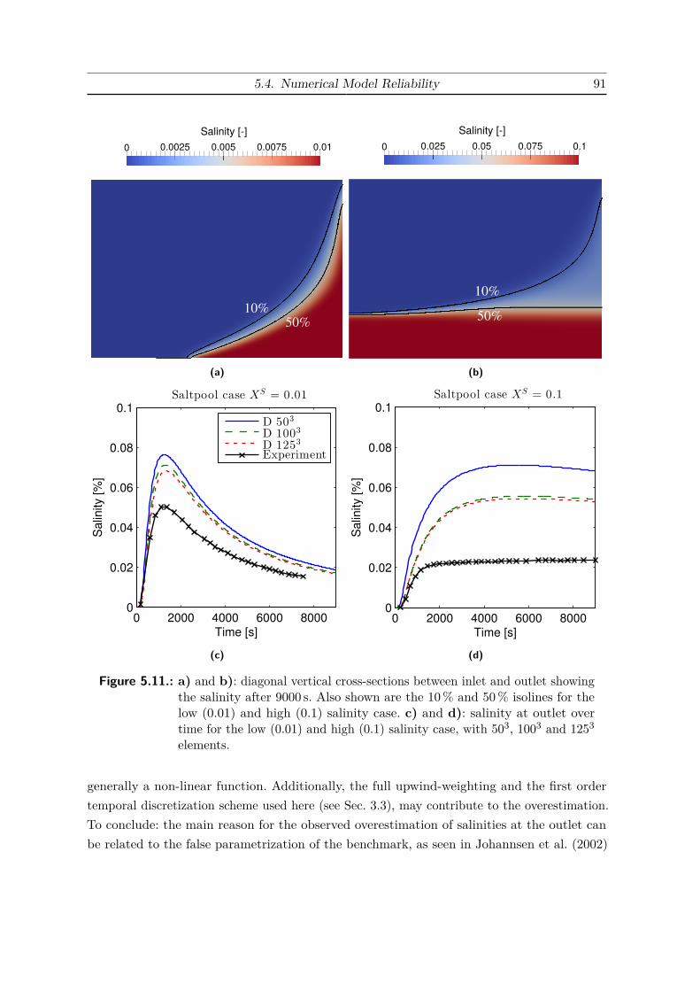
5.4. Numerical Model Reliability 91
0.0025 0.005 0.0075Salinity [-]
0 0.01
10%50%
(a)
0.025 0.05 0.075Salinity [-]
0 0.1
10%
50%
(b)
0 2000 4000 6000 80000
0.02
0.04
0.06
0.08
0.1Saltpool case X
S = 0.01
Time [s]
Sa
linity [
%]
D 503
D 1003
D 1253
Experiment
(c)
0 2000 4000 6000 80000
0.02
0.04
0.06
0.08
0.1Saltpool case XS = 0.1
Sa
linity [
%]
Time [s]
(d)
Figure 5.11.: a) and b): diagonal vertical cross-sections between inlet and outlet showingthe salinity after 9000 s. Also shown are the 10% and 50% isolines for thelow (0.01) and high (0.1) salinity case. c) and d): salinity at outlet overtime for the low (0.01) and high (0.1) salinity case, with 503, 1003 and 1253
elements.
generally a non-linear function. Additionally, the full upwind-weighting and the first ordertemporal discretization scheme used here (see Sec. 3.3), may contribute to the overestimation.To conclude: the main reason for the observed overestimation of salinities at the outlet canbe related to the false parametrization of the benchmark, as seen in Johannsen et al. (2002)
92 5. Large-Scale Investigation of Brine Displacement
and Bastian et al. (2001). A second reason for this observed overestimation of salinity maybe related to the implementation of variable-density flow in DuMux. Both issues should beinvestigated in future work. For the simulations of large scale brine displacement presentedbelow, the results of the saltpool benchmark imply that when considering concentrations asa target variable, these concentrations will be strongly influenced by the highly uncertainparametrization, especially with regard to the dispersivities. However, the overall flow fieldwill react much less sensitively to the variation of salinities, especially to those with a smallvalue. This argument is supported by the qualitative agreement between the experimentalresults and the simulation results of the saltpool benchmark.The simulation of the high density case with 1253 elements is only feasible, with a massiveparallelization. The wall clock time for this case was 10 hours on 120 processes. Unfortunately,a massive parallelization could not be applied to the simulations of the complex geologicalmodel presented below. The heterogeneities and high aspect ratios of the elements made aconvergence of the parallel linear solver impossible.
5.5. Results
The results section is divided into three parts. (i) definition of appropriate target variables, (ii)the results of the scenario analysis (scenario uncertainty), and, (iii) the comparison of modelsof different physical complexity (model uncertainty).
5.5.1. Definition of Target Variables
First, the target variables which will be used to compare the results within this section aredefined. The choice of an effective and efficient conceptual model is closely connected to thetarget variable considered.
• Flow into target aquifers: The target aquifers are defined as all layers located abovethe Rupelian clay barrier, i.e. the Post-Rupelian, Quaternary 2 and Quaternary 1 layers.Different areas are distinguished, over which the flow into the target aquifers is summedup: (i) flow near the salt wall, which comprises flow through the fault zone and flowthrough the Cretaceous dragged up by the salt wall (for ease of notation, both arereferred to as flow through the fault zone), and (ii) flow through the hydrogeologicalwindows in the Rupelian clay barrier. Figure 5.12 shows a view on the interface betweenthe Rupelian clay barrier and the Post-Rupelian layer. Further, the total salt flow intothe more shallow Quarternary 1 and 2 layers is also considered.
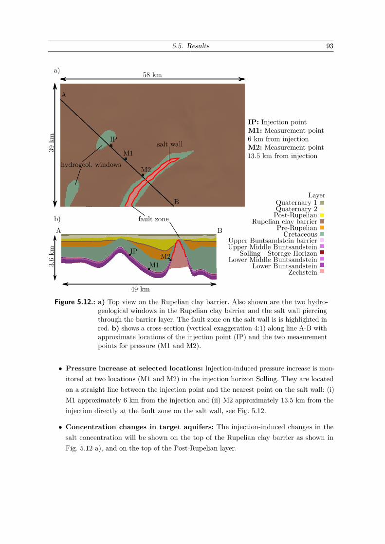
5.5. Results 93
IP: Injection pointM1: Measurement point
M2: Measurement point6 km from injection
13.5 km from injection
a)
b)
M2
M1
IP
fault zone
Layer
ZechsteinLower Buntsandstein
Lower Middle BuntsandsteinSolling - Storage Horizon
Upper Middle BuntsandsteinUpper Buntsandstein barrier
CretaceousPre-Rupelian
Rupelian clay barrierPost-RupelianQuaternary 2Quaternary 1
A B
39km
58 km
49 km
3.6km IP
M1M2
salt wall
hydrogeol. windows
A
B
Figure 5.12.: a) Top view on the Rupelian clay barrier. Also shown are the two hydro-geological windows in the Rupelian clay barrier and the salt wall piercingthrough the barrier layer. The fault zone on the salt wall is is highlighted inred. b) shows a cross-section (vertical exaggeration 4:1) along line A-B withapproximate locations of the injection point (IP) and the two measurementpoints for pressure (M1 and M2).
• Pressure increase at selected locations: Injection-induced pressure increase is mon-itored at two locations (M1 and M2) in the injection horizon Solling. They are locatedon a straight line between the injection point and the nearest point on the salt wall: (i)M1 approximately 6 km from the injection and (ii) M2 approximately 13.5 km from theinjection directly at the fault zone on the salt wall, see Fig. 5.12.
• Concentration changes in target aquifers: The injection-induced changes in thesalt concentration will be shown on the top of the Rupelian clay barrier as shown inFig. 5.12 a), and on the top of the Post-Rupelian layer.
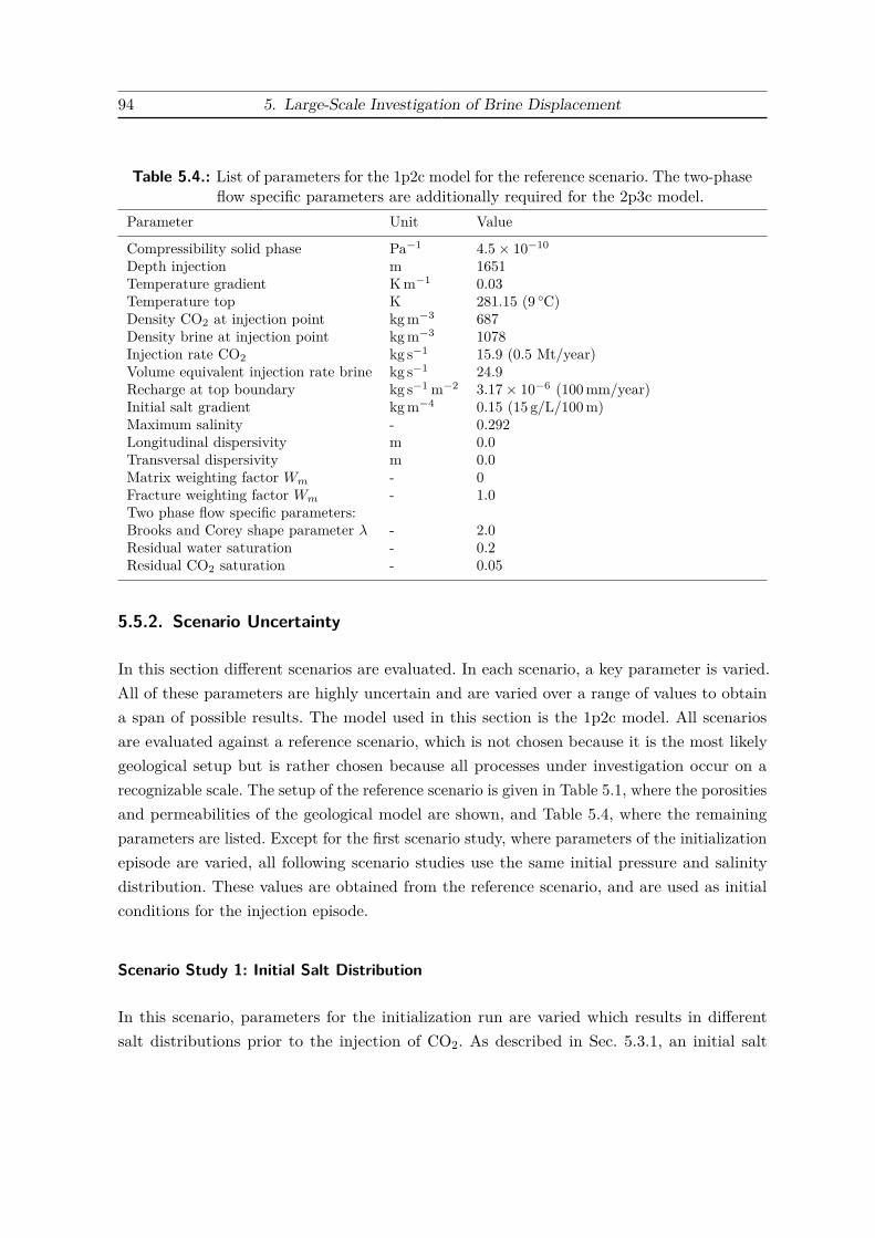
94 5. Large-Scale Investigation of Brine Displacement
Table 5.4.: List of parameters for the 1p2c model for the reference scenario. The two-phaseflow specific parameters are additionally required for the 2p3c model.
Parameter Unit Value
Compressibility solid phase Pa−1 4.5× 10⁻¹⁰
Depth injection m 1651Temperature gradient Km−1 0.03Temperature top K 281.15 (9 ◦C)Density CO2 at injection point kgm−3 687Density brine at injection point kgm−3 1078Injection rate CO2 kg s−1 15.9 (0.5 Mt/year)Volume equivalent injection rate brine kg s−1 24.9Recharge at top boundary kg s−1 m−2 3.17× 10⁻⁶ (100mm/year)Initial salt gradient kgm−4 0.15 (15 g/L/100m)Maximum salinity - 0.292Longitudinal dispersivity m 0.0Transversal dispersivity m 0.0Matrix weighting factor Wm - 0Fracture weighting factor Wm - 1.0Two phase flow specific parameters:Brooks and Corey shape parameter λ - 2.0Residual water saturation - 0.2Residual CO2 saturation - 0.05
5.5.2. Scenario Uncertainty
In this section different scenarios are evaluated. In each scenario, a key parameter is varied.All of these parameters are highly uncertain and are varied over a range of values to obtaina span of possible results. The model used in this section is the 1p2c model. All scenariosare evaluated against a reference scenario, which is not chosen because it is the most likelygeological setup but is rather chosen because all processes under investigation occur on arecognizable scale. The setup of the reference scenario is given in Table 5.1, where the porositiesand permeabilities of the geological model are shown, and Table 5.4, where the remainingparameters are listed. Except for the first scenario study, where parameters of the initializationepisode are varied, all following scenario studies use the same initial pressure and salinitydistribution. These values are obtained from the reference scenario, and are used as initialconditions for the injection episode.
Scenario Study 1: Initial Salt Distribution
In this scenario, parameters for the initialization run are varied which results in differentsalt distributions prior to the injection of CO2. As described in Sec. 5.3.1, an initial salt
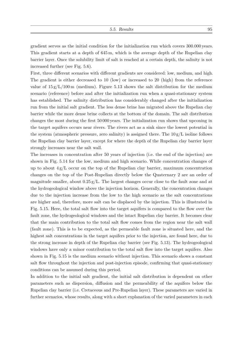
5.5. Results 95
gradient serves as the initial condition for the initialization run which covers 300.000 years.This gradient starts at a depth of 645m, which is the average depth of the Rupelian claybarrier layer. Once the solubility limit of salt is reached at a certain depth, the salinity is notincreased further (see Fig. 5.6).First, three different scenarios with different gradients are considered: low, medium, and high.The gradient is either decreased to 10 (low) or increased to 20 (high) from the referencevalue of 15 g/L/100m (medium). Figure 5.13 shows the salt distribution for the mediumscenario (reference) before and after the initialization run when a quasi-stationary systemhas established. The salinity distribution has considerably changed after the initializationrun from the initial salt gradient. The less dense brine has migrated above the Rupelian claybarrier while the more dense brine collects at the bottom of the domain. The salt distributionchanges the most during the first 50 000 years. The initialization run shows that upconing inthe target aquifers occurs near rivers. The rivers act as a sink since the lowest potential inthe system (atmospheric pressure, zero salinity) is assigned there. The 10 g/L isoline followsthe Rupelian clay barrier layer, except for where the depth of the Rupelian clay barrier layerstrongly increases near the salt wall.The increases in concentration after 50 years of injection (i.e. the end of the injection) areshown in Fig. 5.14 for the low, medium and high scenario. While concentration changes ofup to about 4 g/L occur on the top of the Rupelian clay barrier, maximum concentrationchanges on the top of the Post-Rupelian directly below the Quaternary 2 are an order ofmagnitude smaller, about 0.25 g/L. The largest changes occur close to the fault zone and atthe hydrogeological window above the injection horizon. Generally, the concentration changesdue to the injection increase from the low to the high scenario as the salt concentrationsare higher and, therefore, more salt can be displaced by the injection. This is illustrated inFig. 5.15. Here, the total salt flow into the target aquifers is compared to the flow over thefault zone, the hydrogeological windows and the intact Rupelian clay barrier. It becomes clearthat the main contribution to the total salt flow comes from the region near the salt wall(fault zone). This is to be expected, as the permeable fault zone is situated here, and thehighest salt concentrations in the target aquifers prior to the injection, are found here, due tothe strong increase in depth of the Rupelian clay barrier (see Fig. 5.13). The hydrogeologicalwindows have only a minor contribution to the total salt flow into the target aquifers. Alsoshown in Fig. 5.15 is the medium scenario without injection. This scenario shows a constantsalt flow throughout the injection and post-injection episode, confirming that quasi-stationaryconditions can be assumed during this period.In addition to the initial salt gradient, the initial salt distribution is dependent on otherparameters such as dispersion, diffusion and the permeability of the aquifers below theRupelian clay barrier (i.e. Cretaceous and Pre-Rupelian layer). These parameters are varied infurther scenarios, whose results, along with a short explanation of the varied parameters in each
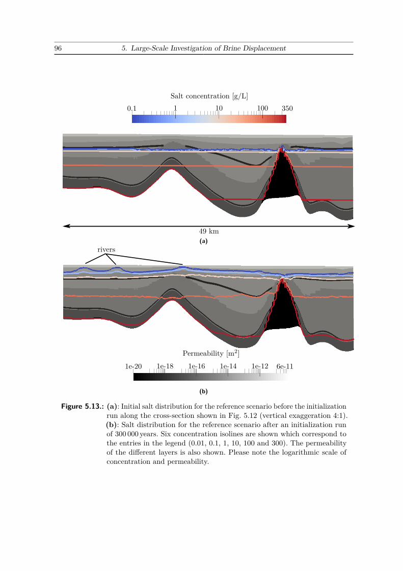
96 5. Large-Scale Investigation of Brine Displacement
1 10 100Salt concentration [g/L]
0.1 350
49 km(a)
1e-18 1e-16 1e-14 1e-12Permeability [m2]
1e-20 6e-11
rivers
(b)
Figure 5.13.: (a): Initial salt distribution for the reference scenario before the initializationrun along the cross-section shown in Fig. 5.12 (vertical exaggeration 4:1).(b): Salt distribution for the reference scenario after an initialization runof 300 000 years. Six concentration isolines are shown which correspond tothe entries in the legend (0.01, 0.1, 1, 10, 100 and 300). The permeabilityof the different layers is also shown. Please note the logarithmic scale ofconcentration and permeability.
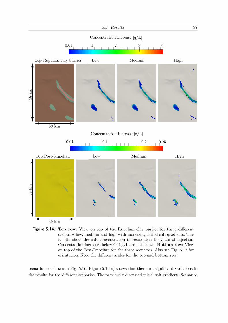
5.5. Results 97
1 2 3
Concentration increase [g/L]
0.01 4
39 km
58km
Top Rupelian clay barrier Low Medium High
0.1 0.2
Concentration increase [g/L]
0.01 0.25
39 km
58km
Top Post-Rupelian Low Medium High
Figure 5.14.: Top row: View on top of the Rupelian clay barrier for three differentscenarios low, medium and high with increasing initial salt gradients. Theresults show the salt concentration increase after 50 years of injection.Concentration increases below 0.01 g/L are not shown. Bottom row: Viewon top of the Post-Rupelian for the three scenarios. Also see Fig. 5.12 fororientation. Note the different scales for the top and bottom row.
scenario, are shown in Fig. 5.16. Figure 5.16 a) shows that there are significant variations inthe results for the different scenarios. The previously discussed initial salt gradient (Scenarios
98 5. Large-Scale Investigation of Brine Displacement
0 20 40 60 80 1000
0.2
0.4
0.6
0.8
1
1.2
Total salt flowSalt
flow
[kg-N
aCl/s]
Time [years]0 20 40 60 80 100
0
0.2
0.4
0.6
0.8
1
1.2
Salt flow over fault zone
Salt
flow
[kg-N
aCl/s]
Time [years]
0 20 40 60 80 1000
0.2
0.4
0.6
0.8
1
1.2
Salt flow over h. windows
Salt
flow
[kg-N
aCl/s]
Time [years]0 20 40 60 80 100
0
0.2
0.4
0.6
0.8
1
1.2
Salt flow over Rupelian clay
Salt
flow
[kg-N
aCl/s]
Time [years]
LowMedium (reference)HighMedium no injection
Figure 5.15.: Total salt flow into target aquifers (top left) over the injection and post-injection period split into salt flow over fault zone (top right), salt flowover hydrogeological windows (bottom left) and salt flow over the intactRupelian clay barrier (bottom right).
2 and 3), the dispersion (large dispersion: Scenario 4), and the reduction of permeability of theCretaceous and Pre-Rupelian (Scenario 6), all have a significant effect on the salt distributionafter the initialization. Therefore, the varied parameters also influence the amount of salt thatis additionally displaced due to the injection on top of the base flow. Scenario 6 illustratesthat the permeabilities of the Cretaceous and Pre-Rupelian layers control the magnitude ofexchange between freshwater and saltwater in locations where the Rupelian Clay barrier isdiscontinuous. Considering for example the reference scenario (Scenario 1) in Fig. 5.16 (a),(b), and (c) shows the decline in the impact of the injection on the amount of displacedsalt in comparison to the amount displaced by the base flow over the injection period. Thecontribution of the injection becomes gradually smaller for the shallower aquifers, while the

5.5. Results 99
1 2 3 4 5 6 70
0.5
1
1.5
2
2.5
Salt flow into target aquifers
Cum.salt
mass
[MT-N
aCl]
Scenario No.
(a)
1 2 3 4 5 6 70
0.5
1
1.5
2
2.5
Scenario No.
Cum.salt
mass
[MT-N
aCl]
Salt flow into Quaternary 2
InjectionNo injection
(b)
1 2 3 4 5 6 70
0.5
1
1.5
2
2.5
Salt flow into Quaternary 1
Cum.salt
mass
[MT-N
aCl]
Scenario No.
(c)
Scenario Description1 Reference (medium)2 Initial salt gradient (low): 10 g/L/100m3 Initial salt gradient (high): 20 g/L/100m4 Dispersion large: αl=70m, αt=7m5 Dispersion small: αl=2m, αt=0.2m6 Factor 10 reduction of
permeability of intermediateaquifers (Cretaceous, Pre-Rupelian)
7 No molecular diffusion
(d)
Figure 5.16.: The cumulative salt flow for a period of 100 years (injection + post injection)into the Tertiary Post-Rupelian layer (a), Quaternary 2 layer (b) andQuaternary 1 layer (c) with and without injection. The scenario numbersalong with short explanations of the varied parameters are given in (d).
base flow stays more or less constant across the target aquifers. This can be explained by thelow salt concentrations found in the bottom of the Quaternary 1 and 2 aquifers, prior to theinjection, compared to higher salt concentrations at the bottom of the Tertiary Post-Rupelianlayer (Fig. 5.16 (a)). The base flow (i.e no injection) of salt is almost the same across all layersof the target aquifers for a specific scenario. This again shows that, for each variation of aparameter, a quasi-stationary solution has evolved with a constant salt flow across the target

100 5. Large-Scale Investigation of Brine Displacement
aquifers.
Scenario Study 2: Boundary Conditions
In this section, three different boundary conditions for the lateral boundaries of the innerdomain are compared. The reference scenario uses a domain extension which results in aninfinite aquifer behavior, as already described above. The other two scenarios use a no-flowand a Dirichlet boundary condition (hydrostatic) respectively, on the lateral boundary of theinner domain. The results of these scenarios are shown in Fig. 5.17. It can be seen that the
0 20 40 60 80 100
0
0.2
0.4
0.6
0.8
1
Total mass flow
Mass
flow
/injectionrate
[-]
Time [years]0 20 40 60 80 100
0
0.2
0.4
0.6
0.8
1
Time [years]
Mass
flow
/injectionrate
[-]
Mass flow over fault zone
Infinite aquiferNo flowDirichlet
Figure 5.17.: Left: Total mass flow into the target aquifers normalized by the injectionrate. Right: Mass flow over fault zone into the target aquifers.
choice of the lateral boundary conditions strongly influences the overall flow regime. For theno flow scenario considerably more fluid is displaced vertically than for the Dirichlet scenario.The reference scenario with an infinite aquifer boundary condition is somewhere in the middleof the other two scenarios. This is expected as more storage capacity for the displaced brine isavailable in the extended aquifers than for the no flow scenario and a stronger resistance toflow at the lateral boundaries is established than in the case of the Dirichlet scenario. For theinfinite aquifer scenario, the total flow into the target aquifers reaches a level of about 60% ofthe injection rate. The rest is stored within the compressible fluid and rock phases.
Scenario Study 3: Barrier Rock Permeability
Within this scenario, the permeability of the layer confining the injection layer, i.e. UpperBuntsandstein barrier, is varied over several orders of magnitude. The results are presented in
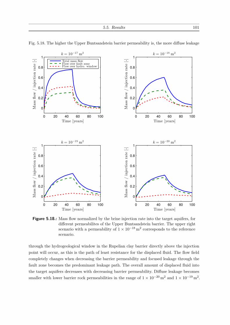
5.5. Results 101
Fig. 5.18. The higher the Upper Buntsandstein barrier permeability is, the more diffuse leakage
0 20 40 60 80 100
0
0.2
0.4
0.6
0.8
1
k = 10−17 m2
Mass
flow
/injectionrate
[-]
Time [years]
Total mass flowFlow over fault zoneFlow over hydro. window
0 20 40 60 80 100
0
0.2
0.4
0.6
0.8
1
k = 10−18 m2
Mass
flow
/injectionrate
[-]
Time [years]
0 20 40 60 80 100
0
0.2
0.4
0.6
0.8
1
k = 10−19 m2
Mass
flow
/injectionrate
[-]
Time [years]0 20 40 60 80 100
0
0.2
0.4
0.6
0.8
1
k = 10−20 m2
Mass
flow
/injectionrate
[-]
Time [years]
Figure 5.18.: Mass flow normalized by the brine injection rate into the target aquifers, fordifferent permeabilites of the Upper Buntsandstein barrier. The upper rightscenario with a permeability of 1× 10⁻¹⁸ m2 corresponds to the referencescenario.
through the hydrogeological window in the Rupelian clay barrier directly above the injectionpoint will occur, as this is the path of least resistance for the displaced fluid. The flow fieldcompletely changes when decreasing the barrier permeability and focused leakage through thefault zone becomes the predominant leakage path. The overall amount of displaced fluid intothe target aquifers decreases with decreasing barrier permeability. Diffuse leakage becomessmaller with lower barrier rock permeabilities in the range of 1× 10⁻²⁰ m2 and 1× 10⁻¹⁹ m2.
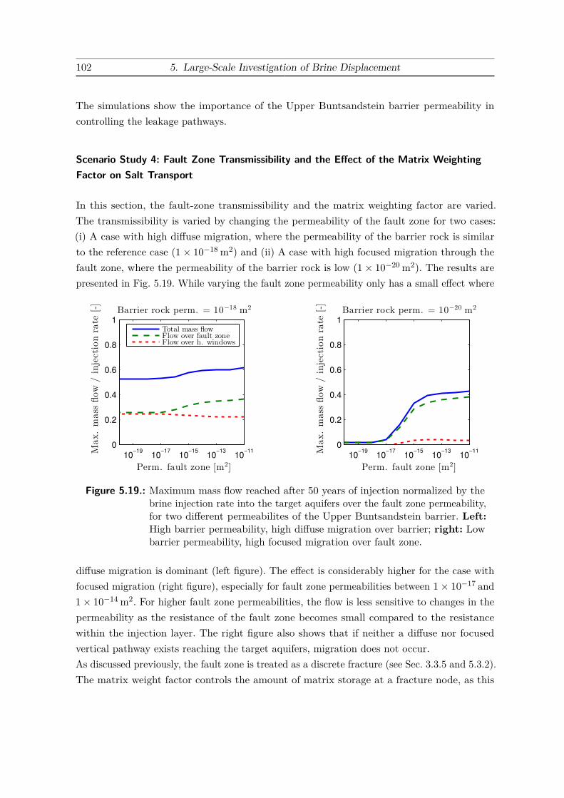
102 5. Large-Scale Investigation of Brine Displacement
The simulations show the importance of the Upper Buntsandstein barrier permeability incontrolling the leakage pathways.
Scenario Study 4: Fault Zone Transmissibility and the Effect of the Matrix WeightingFactor on Salt Transport
In this section, the fault-zone transmissibility and the matrix weighting factor are varied.The transmissibility is varied by changing the permeability of the fault zone for two cases:(i) A case with high diffuse migration, where the permeability of the barrier rock is similarto the reference case (1× 10⁻¹⁸ m2) and (ii) A case with high focused migration through thefault zone, where the permeability of the barrier rock is low (1× 10⁻²⁰ m2). The results arepresented in Fig. 5.19. While varying the fault zone permeability only has a small effect where
10−19
10−17
10−15
10−13
10−11
0
0.2
0.4
0.6
0.8
1
Barrier rock perm. = 10−18 m2
Max.mass
flow
/injectionrate
[-]
Perm. fault zone [m2]
Total mass flowFlow over fault zoneFlow over h. windows
10−19
10−17
10−15
10−13
10−11
0
0.2
0.4
0.6
0.8
1
Barrier rock perm. = 10−20 m2
Max.mass
flow
/injectionrate
[-]
Perm. fault zone [m2]
Figure 5.19.: Maximum mass flow reached after 50 years of injection normalized by thebrine injection rate into the target aquifers over the fault zone permeability,for two different permeabilites of the Upper Buntsandstein barrier. Left:High barrier permeability, high diffuse migration over barrier; right: Lowbarrier permeability, high focused migration over fault zone.
diffuse migration is dominant (left figure). The effect is considerably higher for the case withfocused migration (right figure), especially for fault zone permeabilities between 1× 10⁻¹⁷ and1× 10−14 m2. For higher fault zone permeabilities, the flow is less sensitive to changes in thepermeability as the resistance of the fault zone becomes small compared to the resistancewithin the injection layer. The right figure also shows that if neither a diffuse nor focusedvertical pathway exists reaching the target aquifers, migration does not occur.As discussed previously, the fault zone is treated as a discrete fracture (see Sec. 3.3.5 and 5.3.2).The matrix weight factor controls the amount of matrix storage at a fracture node, as this

5.5. Results 103
node is shared by the fracture and the matrix. If set to zero, the storage of the salt componentonly comprises the fracture storage term and the storage term of the matrix is neglected atthe node. The effect of the matrix weighting factor for the fault zone is compared for twoscenarios: Wm = 0, i.e. fracture storage only, which is the reference scenario, and Wm = 1, i.e.the fracture and the matrix storage term are considered at the node. The results are presentedin Fig. 5.20. For the reference scenario (Wm = 0), the left plot shows that the volume flow is
0 20 40 60 80 1000
0.2
0.4
0.6
0.8
1
Volume flow over fault zone
Vol.
flow/injectionrate
[-]
Time [Years]0 20 40 60 80 100
0
0.2
0.4
0.6
0.8
1
Salt flow over fault zone
Salt
flow
[kg/s]
Time [Years]
Wm = 1Wm = 0 (reference)
Figure 5.20.: Left: Volumetric flow normalized by injection rate into target aquifersthrough the fault zone. Right: Salt flow into target aquifers through faultzone.
lower and the salt flow on the right plot is slightly higher. This is conservative, as required,with respect to an increased transport velocity for the salt component (see Sec. 3.3.5). If Wm
is set to zero, the transport velocity (per area of fluid) of the salt increases. This then meansthat the weight and therefore gravitational force of the brine column within the fault zonewill increase faster. This leads to an increase in the resistive forces, meaning higher pressuresare required in order to push the heavy brine upwards. This increased resistance explainswhy the overall volume flow is lower for the reference scenario. This effect is a consequenceof the variable-density transport of salt. However, the overall effect of the matrix weightingfactor is rather small but can be higher for scenarios where focused leakage through the faultzone is predominant, i.e. for permeabilities of the Upper Buntsandstein barrier smaller than1× 10−19 m2.

104 5. Large-Scale Investigation of Brine Displacement
5.5.3. Model Uncertainty (Recognized ignorance)
The results of four different model comparisons are shown in this section. All comparisons arecarried out against the 1p2c model with the parametrization of the reference scenario givenin Table 5.1 and Table 5.4. As a target variable, the volume flow into the target aquifers ischosen, as this indicates how well the flow fields match. In some comparisons, the pressurebuildup at the measurement points M1 and M2, shown in Fig. 5.12, is also used.
Model Comparison 1: Neglecting Salt Transport
In this comparison, the effects of neglecting salt transport and therefore neglecting the effectsof variable-density flow are investigated, by applying the 1p1c model which neglects salttransport, as opposed to the 1p2c reference model. In the 1p1c model, the salinity is set as apseudo component (similar to temperature) influencing the brine density and viscosity, butheld as a fixed value throughout the simulation. A constant salinity gradient of 15 g/L/100mis assigned in the 1p1c model, similar to the condition shown in Fig. 5.13 a). Since the 1p1cmodel does not require the initialization episode, the results are much faster to obtain than incase of the 1p2c reference model. Brine is injected at a rate of 25.2 kg/s in the 1p1c modelwhich is the volume equivalent rate corresponding to the 24.9 kg/s injected in the 1p2c modeldue to different densities at the injection point (1p1c: 1091 kg/m3; 1p2c: 1078 kg/m3). The aimis to investigate whether both models lead to a similar flow fields. The results for the flow intothe target aquifer are shown in Fig. 5.21. The total volume flow is higher by approximately5% for the 1p1c model than that of the 1p2c model. For the 1p1c model, the volume flowover the fault zone and the hydrogeological windows starts at a value below, and above zero,respectively (see Fig. 5.21). This is caused by the base flow induced by the recharge boundaryconditions on the top boundary. For the reference 1p2c model, the overall exchange of waterbetween the target aquifers and the layers below the Rupelian clay barrier is much smallerthan for the 1p1c, as the saltwater needs to be moved against the gravitational forces. For the1p1c model, the base flow and the injection-induced flow have the same order of magnitude,whereas base flow in the 1p2c model is negligible compared to the injection-induced flow. Onthe bottom row of Fig. 5.21, the pressure increase at M1 and M2 are shown (see Fig. 5.12 forthe approximate locations). The pressure increase at 6 km from the injection (M1) is almostthe same for both models, as the brine viscosity in the injection layer is similar. However, atthe fault zone, the pressure increase for the 1p2c is higher by a factor of approximately three,compared with the 1p1c model. This is due to the increasing weight of the ascending brinewithin the fault zone, leading to an increasing resistance. This is a result of salt transport andthe associated density changes.
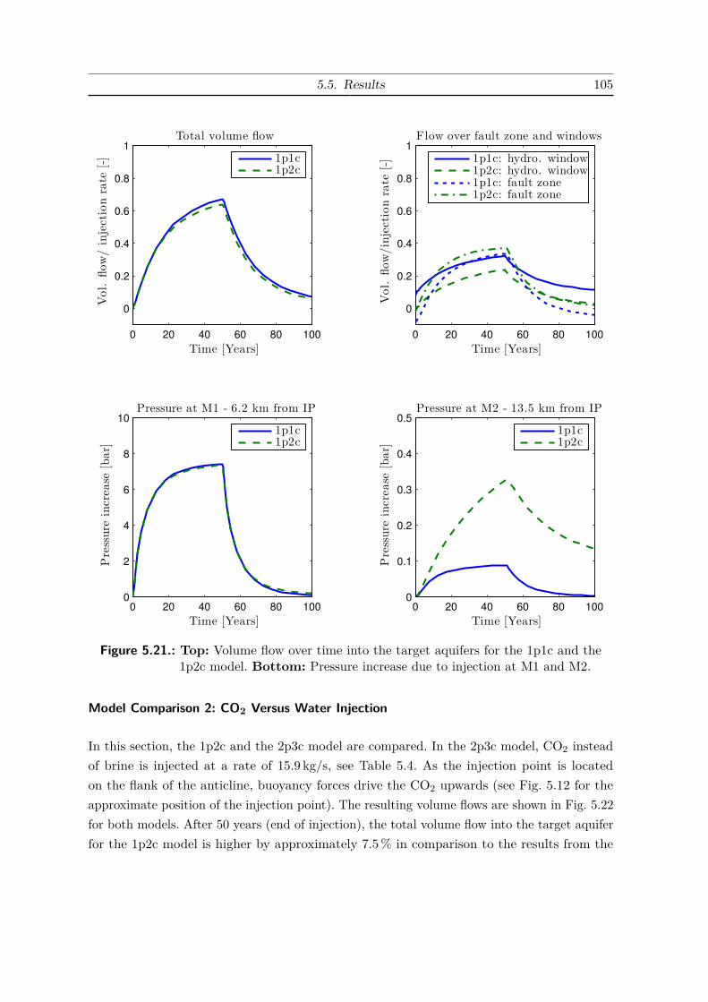
5.5. Results 105
0 20 40 60 80 100
0
0.2
0.4
0.6
0.8
1
Total volume flow
Vol.
flow/injectionrate
[-]
Time [Years]
1p1c1p2c
0 20 40 60 80 100
0
0.2
0.4
0.6
0.8
1
Flow over fault zone and windows
Vol.
flow/injectionrate
[-]
Time [Years]
1p1c: hydro. window1p2c: hydro. window1p1c: fault zone1p2c: fault zone
0 20 40 60 80 1000
2
4
6
8
10
Pressure at M1 - 6.2 km from IP
Pressure
increa
se[bar]
Time [Years]
1p1c1p2c
0 20 40 60 80 1000
0.1
0.2
0.3
0.4
0.5
Pressure at M2 - 13.5 km from IP
Pressure
increa
se[bar]
Time [Years]
1p1c1p2c
Figure 5.21.: Top: Volume flow over time into the target aquifers for the 1p1c and the1p2c model. Bottom: Pressure increase due to injection at M1 and M2.
Model Comparison 2: CO2 Versus Water Injection
In this section, the 1p2c and the 2p3c model are compared. In the 2p3c model, CO2 insteadof brine is injected at a rate of 15.9 kg/s, see Table 5.4. As the injection point is locatedon the flank of the anticline, buoyancy forces drive the CO2 upwards (see Fig. 5.12 for theapproximate position of the injection point). The resulting volume flows are shown in Fig. 5.22for both models. After 50 years (end of injection), the total volume flow into the target aquiferfor the 1p2c model is higher by approximately 7.5% in comparison to the results from the

106 5. Large-Scale Investigation of Brine Displacement
0 20 40 60 80 100
0
0.2
0.4
0.6
0.8
1
Total volume flow
Time [Years]
Vol.
flow/injectionrate
[-]
2p3c1p2c
0 20 40 60 80 100
0
0.2
0.4
0.6
0.8
1
Flow over fault zone and windows
Time [Years]
Vol.
flow/injectionrate
[-]
2p3c: h. windows1p2c: h. windows2p3c: fault zone1p2c: fault zone
Figure 5.22.: Volume flow over time into the target aquifers for the 2p3c and the 1p2cmodel.
2p3c model. The right figure shows that the volume flow across the hydrogeological windowsand the fault zone are in good agreement for both models. The the slightly reduced volumeflow for the 2p3c model compared to the 1p2c model is due to the rise in pressure near theinjection, which causes the density of CO2 to increase, leading to a smaller brine flow into thetarget aquifers.
Model Comparison 3: Simplifying the Geometry
This comparison deals with a major simplification of the geometry. The reference 1p2c modelis called “complex case“, while the simplified geometry is referred to as “generic case“. Inthe generic case, the complex geometry is converted into a simple stratified system with thelayering orthogonal to the direction of gravity as shown in Fig. 5.23. The target aquifersare removed and replaced by a Dirichlet boundary condition with a constant hydrostaticpressure and zero salinity above the Rupelian clay barrier. Therefore, no base flow establishesas hydrostatic conditions are assumed within the domain, along with a linear salinity gradientsimilar to the one prescribed initially for the complex case before the initialization run (15 g/L).Due to the simple geometry and boundary conditions no initialization run is required priorto the injection. The salt wall is implemented at the boundary of the model domain alongwith the fault zone marked in red in Fig. 5.23. The lateral boundary conditions are infiniteaquifers, like those in the complex model. The geometrical information required for the genericmodel’s setup consists only of the layer thicknesses, the distances of geological features, andthe areas of the hydrogeological windows. They are estimated based on the complex geometry.
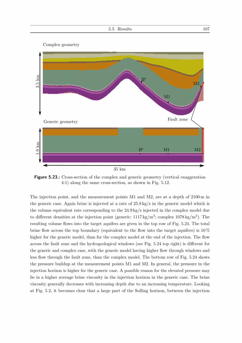
5.5. Results 107
IP M2M1
Generic geometry
Complex geometry
M1
IPM2
35 km
Fault zone
3.5km
1.9km
Figure 5.23.: Cross-section of the complex and generic geometry (vertical exaggeration4:1) along the same cross-section, as shown in Fig. 5.12.
The injection point, and the measurement points M1 and M2, are at a depth of 2100m inthe generic case. Again brine is injected at a rate of 25.8 kg/s in the generic model which isthe volume equivalent rate corresponding to the 24.9 kg/s injected in the complex model dueto different densities at the injection point (generic: 1117 kg/m3; complex 1078 kg/m3). Theresulting volume flows into the target aquifers are given in the top row of Fig. 5.24. The totalbrine flow across the top boundary (equivalent to the flow into the target aquifers) is 10%higher for the generic model, than for the complex model at the end of the injection. The flowacross the fault zone and the hydrogeological windows (see Fig. 5.24 top right) is different forthe generic and complex case, with the generic model having higher flow through windows andless flow through the fault zone, than the complex model. The bottom row of Fig. 5.24 showsthe pressure buildup at the measurement points M1 and M2. In general, the pressure in theinjection horizon is higher for the generic case. A possible reason for the elevated pressure maylie in a higher average brine viscosity in the injection horizon in the generic case. The brineviscosity generally decreases with increasing depth due to an increasing temperature. Lookingat Fig. 5.2, it becomes clear that a large part of the Solling horizon, between the injection
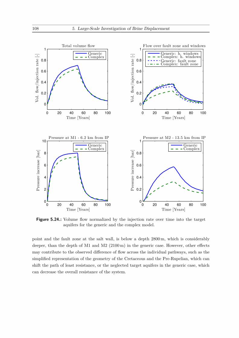
108 5. Large-Scale Investigation of Brine Displacement
0 20 40 60 80 100
0
0.2
0.4
0.6
0.8
1
Total volume flow
Time [Years]
Vol.
flow/injectionrate
[-]
GenericComplex
0 20 40 60 80 100
0
0.2
0.4
0.6
0.8
1
Flow over fault zone and windows
Time [Years]
Vol.
flow/injectionrate
[-]
Generic: h. windowsComplex: h. windowsGeneric: fault zoneComplex: fault zone
0 20 40 60 80 1000
2
4
6
8
10
Pressure at M1 - 6.2 km from IP
Time [Years]
Pressure
increa
se[bar]
GenericComplex
0 20 40 60 80 1000
0.2
0.4
0.6
0.8
1
Pressure at M2 - 13.5 km from IP
Time [Years]
Pressure
increa
se[bar]
GenericComplex
Figure 5.24.: Volume flow normalized by the injection rate over time into the targetaquifers for the generic and the complex model.
point and the fault zone at the salt wall, is below a depth 2800m, which is considerablydeeper, than the depth of M1 and M2 (2100m) in the generic case. However, other effectsmay contribute to the observed difference of flow across the individual pathways, such as thesimplified representation of the geometry of the Cretaceous and the Pre-Rupelian, which canshift the path of least resistance, or the neglected target aquifers in the generic case, whichcan decrease the overall resistance of the system.
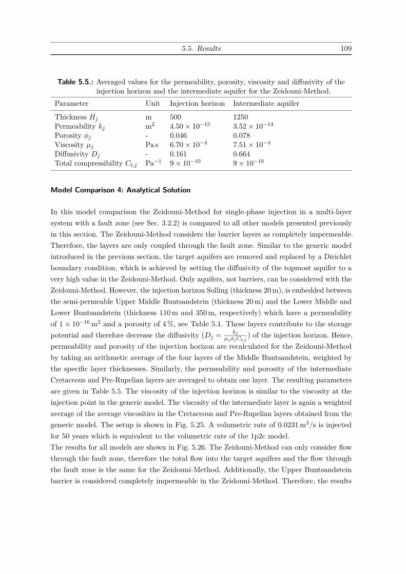
5.5. Results 109
Table 5.5.: Averaged values for the permeability, porosity, viscosity and diffusivity of theinjection horizon and the intermediate aquifer for the Zeidouni-Method.
Parameter Unit Injection horizon Intermediate aquifer
Thickness Hj m 500 1250Permeability kj m2 4.50× 10⁻¹⁵ 3.52× 10⁻¹⁴
Porosity φj - 0.046 0.078Viscosity µj Pa s 6.70× 10⁻⁴ 7.51× 10⁻⁴
Diffusivity Dj - 0.161 0.664Total compressibility Ct,j Pa−1 9× 10⁻¹⁰ 9× 10⁻¹⁰
Model Comparison 4: Analytical Solution
In this model comparison the Zeidouni-Method for single-phase injection in a multi-layersystem with a fault zone (see Sec. 3.2.2) is compared to all other models presented previouslyin this section. The Zeidouni-Method considers the barrier layers as completely impermeable.Therefore, the layers are only coupled through the fault zone. Similar to the generic modelintroduced in the previous section, the target aquifers are removed and replaced by a Dirichletboundary condition, which is achieved by setting the diffusivity of the topmost aquifer to avery high value in the Zeidouni-Method. Only aquifers, not barriers, can be considered with theZeidouni-Method. However, the injection horizon Solling (thickness 20m), is embedded betweenthe semi-permeable Upper Middle Buntsandstein (thickness 20m) and the Lower Middle andLower Buntsandstein (thickness 110m and 350m, respectively) which have a permeabilityof 1× 10⁻¹⁶ m2 and a porosity of 4%, see Table 5.1. These layers contribute to the storagepotential and therefore decrease the diffusivity (Dj = kj
µjφjCt,j) of the injection horizon. Hence,
permeability and porosity of the injection horizon are recalculated for the Zeidouni-Methodby taking an arithmetic average of the four layers of the Middle Buntsandstein, weighted bythe specific layer thicknesses. Similarly, the permeability and porosity of the intermediateCretaceous and Pre-Rupelian layers are averaged to obtain one layer. The resulting parametersare given in Table 5.5. The viscosity of the injection horizon is similar to the viscosity at theinjection point in the generic model. The viscosity of the intermediate layer is again a weightedaverage of the average viscosities in the Cretaceous and Pre-Rupelian layers obtained from thegeneric model. The setup is shown in Fig. 5.25. A volumetric rate of 0.0231m3/s is injectedfor 50 years which is equivalent to the volumetric rate of the 1p2c model.The results for all models are shown in Fig. 5.26. The Zeidouni-Method can only consider flowthrough the fault zone, therefore the total flow into the target aquifers and the flow throughthe fault zone is the same for the Zeidouni-Method. Additionally, the Upper Buntsandsteinbarrier is considered completely impermeable in the Zeidouni-Method. Therefore, the results

110 5. Large-Scale Investigation of Brine Displacement
fault zone
infin
iteaq
uifer
no-flow
boun
dary
x=0x=13,500 m
intermediate aquifers
injection horizon
confining layer
target aquifers
Qwell
confining layer
Upper Buntsandstein barrier
Rupelian clay barrier
Middle and
Pre-Rupelian and
Lower Buntsandstein
Cretaceous
infinite diffusivity
Figure 5.25.: Model setup for the Zeidouni-Method with two permeable layers (injectionhorizon and intermediate aquifers) and the target aquifers with infinitediffusivity.
of the Zeidouni-Method are the same if this parameter is varied, as shown in Fig. 5.26.For a permeability of 1× 10⁻¹⁸ m2 of the Upper Buntsandstein barrier, diffuse migrationis significant, as seen in the top row. The total volumetric flow is underestimated by theZeidouni-Method whereas the volumetric flow over the fault zone is overestimated. The casewhen focused migration over the fault zone is predominant (bottom row Fig 5.26) is in betteragreement with the assumptions of the Zeidouni-Method. Here, the volumetric flow into thetarget aquifers is higher for the Zeidouni-Method than for the numerical models. The mainreason for this is the different realization of the injection horizon. In the numerical model, thesemi-permeable layers surrounding the Solling injection horizon provide additional storagepotential which reduces the diffusivity of the injection complex. In the Zeidouni-Method, areduction of the diffusivity is achieved by reducing the permeability of the injection horizonthrough the averaging process described above. However, this procedure is not physicallyequivalent with the numerical model and may therefore not generally be expected to deliversimilar results. Neglecting the layers surrounding the Solling for the Zeidouni-Method wouldlead to a very large diffusivity of 0.913 causing a strong overestimation of the volume flowinto the target aquifers. This overestimation is shown in the right plot of the bottom row inFig. 5.26.Table 5.6 summarizes the comparison between the different models. It shows the cumulativedisplaced volumes into the target aquifers during the injection period. The overall agreementis best for the low Upper Buntsandstein barrier permeability (1× 10⁻²⁰ m2), where focusedleakage over the fault zone is the main vertical migration pathway. If both diffuse migrationover the barrier rock, and focused migration over the fault zone occur, a larger variation inthe results can be observed, as the distribution of flow among the different pathways varies.Considering both cases of high and low diffuse migration, the best agreement is observed
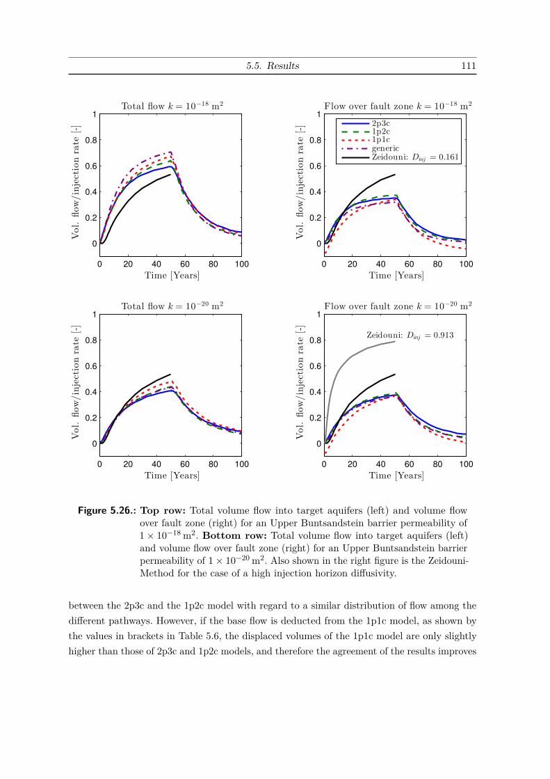
5.5. Results 111
0 20 40 60 80 100
0
0.2
0.4
0.6
0.8
1
Total flow k = 10−18 m2
Vol.
flow/injectionrate
[-]
Time [Years]0 20 40 60 80 100
0
0.2
0.4
0.6
0.8
1
Flow over fault zone k = 10−18 m2
Vol.
flow/injectionrate
[-]
Time [Years]
2p3c1p2c1p1cgenericZeidouni: Dinj = 0.161
0 20 40 60 80 100
0
0.2
0.4
0.6
0.8
1
Total flow k = 10−20 m2
Vol.
flow/injectionrate
[-]
Time [Years]0 20 40 60 80 100
0
0.2
0.4
0.6
0.8
1
Flow over fault zone k = 10−20 m2
Zeidouni: Dinj = 0.913
Vol.
flow/injectionrate
[-]
Time [Years]
Figure 5.26.: Top row: Total volume flow into target aquifers (left) and volume flowover fault zone (right) for an Upper Buntsandstein barrier permeability of1× 10−18 m2. Bottom row: Total volume flow into target aquifers (left)and volume flow over fault zone (right) for an Upper Buntsandstein barrierpermeability of 1× 10⁻²⁰ m2. Also shown in the right figure is the Zeidouni-Method for the case of a high injection horizon diffusivity.
between the 2p3c and the 1p2c model with regard to a similar distribution of flow among thedifferent pathways. However, if the base flow is deducted from the 1p1c model, as shown bythe values in brackets in Table 5.6, the displaced volumes of the 1p1c model are only slightlyhigher than those of 2p3c and 1p2c models, and therefore the agreement of the results improves
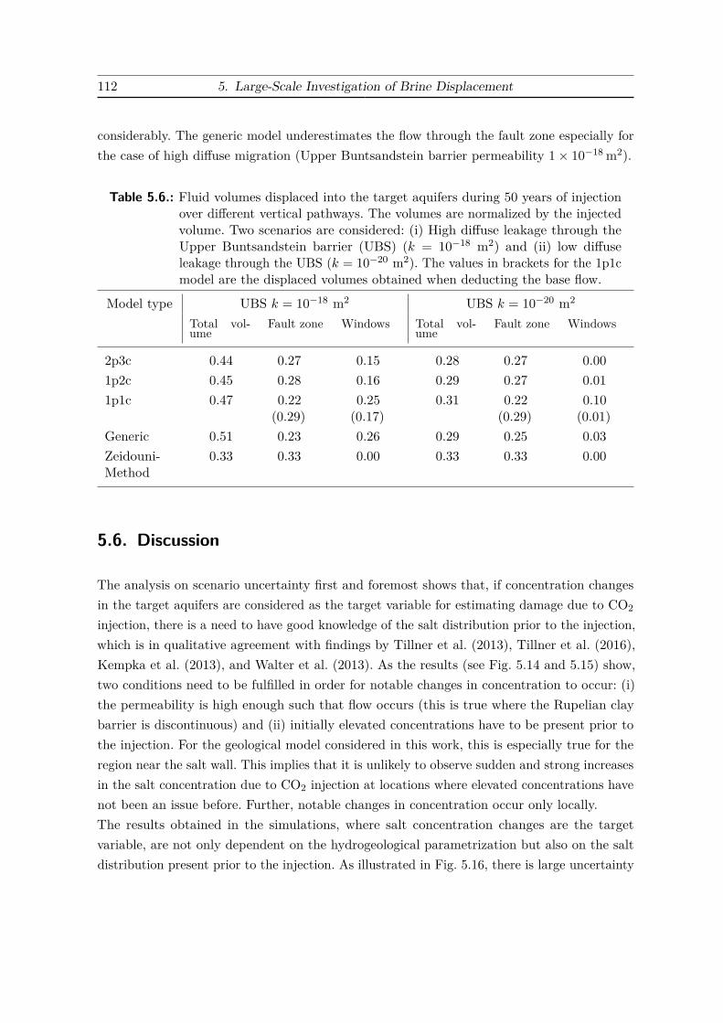
112 5. Large-Scale Investigation of Brine Displacement
considerably. The generic model underestimates the flow through the fault zone especially forthe case of high diffuse migration (Upper Buntsandstein barrier permeability 1× 10⁻¹⁸ m2).
Table 5.6.: Fluid volumes displaced into the target aquifers during 50 years of injectionover different vertical pathways. The volumes are normalized by the injectedvolume. Two scenarios are considered: (i) High diffuse leakage through theUpper Buntsandstein barrier (UBS) (k = 10−18 m2) and (ii) low diffuseleakage through the UBS (k = 10−20 m2). The values in brackets for the 1p1cmodel are the displaced volumes obtained when deducting the base flow.
Model type UBS k = 10−18 m2 UBS k = 10−20 m2
Total vol-ume
Fault zone Windows Total vol-ume
Fault zone Windows
2p3c 0.44 0.27 0.15 0.28 0.27 0.001p2c 0.45 0.28 0.16 0.29 0.27 0.011p1c 0.47 0.22
(0.29)0.25(0.17)
0.31 0.22(0.29)
0.10(0.01)
Generic 0.51 0.23 0.26 0.29 0.25 0.03Zeidouni-Method
0.33 0.33 0.00 0.33 0.33 0.00
5.6. Discussion
The analysis on scenario uncertainty first and foremost shows that, if concentration changesin the target aquifers are considered as the target variable for estimating damage due to CO2
injection, there is a need to have good knowledge of the salt distribution prior to the injection,which is in qualitative agreement with findings by Tillner et al. (2013), Tillner et al. (2016),Kempka et al. (2013), and Walter et al. (2013). As the results (see Fig. 5.14 and 5.15) show,two conditions need to be fulfilled in order for notable changes in concentration to occur: (i)the permeability is high enough such that flow occurs (this is true where the Rupelian claybarrier is discontinuous) and (ii) initially elevated concentrations have to be present prior tothe injection. For the geological model considered in this work, this is especially true for theregion near the salt wall. This implies that it is unlikely to observe sudden and strong increasesin the salt concentration due to CO2 injection at locations where elevated concentrations havenot been an issue before. Further, notable changes in concentration occur only locally.The results obtained in the simulations, where salt concentration changes are the targetvariable, are not only dependent on the hydrogeological parametrization but also on the saltdistribution present prior to the injection. As illustrated in Fig. 5.16, there is large uncertainty

5.6. Discussion 113
regarding different parameters for the initialization run which directly pass on to the resultsobtained after the injection. There is still room for further investigating the uncertainties,with regard to the model complexity and the parametrization, of models aiming to determinenatural pressure, temperature and salinity distributions on a regional scale. For example,the transport of heat is not considered within this work, although a constant geothermalgradient influencing the fluid properties is assumed. A variable temperature distribution canhave a strong influence on the base flow and the salt distribution that establishes duringthe initialization run (Kaiser et al., 2013; Noack et al., 2013). Thereby, the salt wall, whichhas a higher thermal conductivity than the surrounding layers (Magri et al., 2009a) plays animportant role. Future work should evaluate the influence of heat transport on the initial saltdistribution. Magri et al. (2009a) model the evolution of the salt and the temperature field neara salt dome with a 2D numerical model. They introduce a so called “transition zone“ betweenthe salt wall and the surrounding layers. Permeability and porosity values of the transitionzone are higher than those of the the salt wall but lower than those of the surrounding layers.They show that the transition zone slows down the flow of salt into the surrounding layers.The transition zone can be considered equivalent to the fault zone in this work. LBEG (2014)suspect the existence of permeable pathways similar to a fault zone near a salt wall. Makingthis assumption, and considering the results of Magri et al. (2009a), implies that the saltwould dissolve and propagate faster from the salt wall, when considering a permeable faultzone surrounding the salt wall. To this end, there remain many open questions with regard toa realistic parametrization of the near salt wall region.A massive parallelization could help to overcome the high computational demand of theinitialization run, especially if heat transport is to be considered as well. Using the parallelcapabilities of DuMux is not feasible in the current state of the implementation, for the type ofsystem considered in this chapter. The reason lies in the implementation of the parallelization ofthe linear solver, which proves to be very sensitive to the high aspect ratios of the elements andthe layered heterogeneities. These seem to cause badly conditioned matrices on the individualprocesses. A domain decomposition algorithm, which takes into account the connectivitybetween the degrees of freedom, or in other words which “knows“ about the heterogeneitiesmay improve the convergence of the parallel linear solver. For realistic large scale models,considering salt and heat transport, a robust parallelization is necessary for future work.A key aspect when considering the injection of CO2 is the definition of realistic boundaryconditions. Assuming Dirichlet conditions at the lateral boundaries during the injection willlead to an underestimation of the vertical migration of brine. Incorporating no-flow boundarieswithin the inner domain, or extending the model to obtain infinite aquifer conditions will allowsignificantly higher vertical brine flow, as shown in Fig. 5.17. If the top boundary above thetarget aquifers was considered a no-flow boundary, brine flow into the target aquifers wouldbe significantly smaller, similar to the results found by Walter et al. (2012, 2013) or Cihan
114 5. Large-Scale Investigation of Brine Displacement
et al. (2013) where the displaced brine distributes more into the intermediate aquifers belowthe target aquifers.Of similar relevance is the diffuse migration across the barrier layers, especially the barrierlayer sealing the injection layer, (here: Upper Buntsandstein barrier). The results presentedhere show that if the permeability of the Upper Buntsandstein barrier is increased, the verticalleakage of brine increases as well, because the overall vertical resistance decreases. Significantdiffuse migration across the barrier will change the flow regime in the intermediate layers(Cretaceous, Pre-Rupelian) resulting in focused migration, in locations where the Rupelian claybarrier is discontinuous (hydrogeological windows), even if the Upper Buntsandstein barrierbelow is intact (see Fig. 5.18). Diffuse vertical migration is significant for permeabilities higherthan 1× 10⁻¹⁹ m2, which is in good agreement with findings in Birkholzer et al. (2009).Varying the fault zone transmissiblity shows that the injection-induced upward flow is mostsensitive to this parameter when diffuse migration is small, and the resistance from the injectionpoint to the fault zone is in the same range as the resistance over the length of the faultzone. The sensitivity of the leakage rate with respect to the fault zone transmissiblity is smallfor fault zone permeabilities higher than 1× 10⁻¹⁴ m2, even when increasing the fault zonepermeability over several orders of magnitude. Therefore, when assuming a highly permeablefault zone, a simplified geometrical representation of the fault zone, as used in this work,should be sufficient. Focused vertical leakage of highly saline water, which mixes with lesssaline water in the fault zone, leads to an additional resistance against flow. This resistanceis caused by the increasing weight of the saltwater column in the fault zone. The faster thetransport velocity of salt, the faster the resistance will increase. As a result of this resistance,the volume flow through the fault zone decreases. This effect is shown in Fig. 5.20, where thestorage term of the fault zone nodes is manipulated with the matrix weighting factor (Wm). Ahigh storage in the fault zone (Wm = 1) will decrease the transport velocity of the salt, andthe resistance, which results in an increased volume flow and a decreased salt flow over thefault zone, when compared to the reference scenario with a low fault zone storage (Wm = 0).A new hydrostatic equilibrium, which means that the injection-induced flow over the faultceases entirely due to the increasing gravitational force, such as discussed in Oldenburg andRinaldi (2010), is not observed in any of the simulations in this work.Next, the effect of different model assumptions (model uncertainty) is discussed. In the firstmodel comparison, the transport of salt and, thus, variable-density flow, is neglected. Thecorresponding 1p1c model does not require a complex and costly initialization run. Obviously,concentration changes cannot be considered as a target variable, but still relevant informationon volume flow into the target aquifers can be obtained, which may be a useful target variablefor optimizing a pressure management concept. In the 1p1c model, the total volume flow isonly slightly higher than in the 1p2c model (see Fig. 5.21, top left). However, when lookingat the individual flow paths (see Fig. 5.21, top right), it is observed that the base flow in

5.6. Discussion 115
the 1p1c model is much higher than in the 1p2c model. The base flow in the 1p1c model isstill smaller than the injection-induced flow, but it has the same order of magnitude. In the1p2c model, the exchange of fluid between the saltwater and freshwater aquifers is reduced, asan effect of the additional resistance caused by an increase in the gravitational force, whensaltwater is transported upwards. If the base flow is deducted from the leakage rates, theagreement between the 1p1c and the 1p2c reference model, regarding the displaced volumesinto the target aquifers, significantly improves (see Table. 5.6). When looking at the pressures(bottom row of Fig. 5.21) at the measurement point M1 (6.2 km from the injection), which arein very good agreement for the two models, it becomes clear that the overall resistance in theinjection layer is met, by making the salinity a pseudo component. In contrast, the pressureincrease at M2 (13.5 km from the injection at the fault zone) is about three times as high forthe 1p2c model as for the 1p1c model, which can be attributed to the increased resistance dueto the focused vertical transport of salt through the fault zone. Hence, the transport of salt isimportant to consider if pressure increase is a target variable.The second assumption that was investigated concerns the effect of injecting brine insteadof supercritical CO2 at a volume-equivalent rate. The total volume displaced into the targetaquifers during 50 years of injection is 4.7% higher for the 1p2c model than for the 2p3cmodel (see Table 5.6, high diffuse leakage scenario). With regard to the distribution of flowamong the vertical pathways (hydrogeological windows and fault zone), the models are ingood agreement. The injection of brine instead of CO2 is therefore a reasonable conservativeassumption that simplifies the physics considerably. This assumption has also been previouslydiscussed in the literature for example by Cihan et al. (2013).The next assumption deals with simplifying the complex geometry of the geological model. Asimpler generic geological model may be advantageous in many cases, as the effort of settingup the geological model is reduced and the implementation of geological features is faster.For example, if the uncertainty in the location of fault zones were included within a riskassessment approach, a simpler generic geological model would allow for a faster analysisof this uncertainty. However, if the location of the geological features is known, then it isimportant to have good estimates of the horizontal and vertical distances and transmissibilitiesbetween features since these determine the main flow paths. Additionally, for the geologicalmodel considered here, the viscosity differences due to the varying depth of the injection layerin the complex model can lead to a different resistance compared with the generic model.The same arguments hold for analytical solutions which also rely on a simplified geometricaldescription of the geological model. The results show that the total flow into the target aquifersfor the generic geometry is overestimated by about 13% for the high diffuse leakage scenarioin comparison to the 1p2c reference model with the complex geological model, see Table 5.6.The results of the generic and the complex geological models are in better agreement for lowdiffuse migration over the Upper Buntsandstein barrier, also see Table 5.6. As discussed above,

116 5. Large-Scale Investigation of Brine Displacement
the uncertainty related to the simulated salt distribution prior to the injection is quite highfor the complex geological model, and in reality, there will probably not be sufficient data tocalibrate the simulation results to. Therefore, using conservative assumptions, as presented inWalter et al. (2012) or Cihan et al. (2013), with a generic geometry can be justified in thelight of sparse data availability. The salt concentration at the saltwater - freshwater interfacewill then strongly influence the results of a risk assessment.Finally, comparing the results of the numerical models to the Zeidouni-Method (Zeidouni, 2012)reveals first and foremost the importance of considering the semi-permeable layers, here definedas the layers with a permeability of 1× 10⁻¹⁶ m2, that surround the injection horizon Solling.Their contribution to the overall storage of displaced brine is high which causes a reductionof vertical flow during the injection period. When including the layers of the Middle andLower Buntsandstein into the Zeidouni-Method an averaging of the properties of these layersis performed in order to obtain one injection layer with a more realistic diffusivity than theone obtained when solely considering the Solling layer. The results given in Fig. 5.26 show thatthe Zeidouni-Method underestimates flow for the case when diffuse migration across the UpperBuntsandstein barrier is significant and overestimates flow if focused migration over the faultzone is the dominant migration pathway. The latter scenario is in better agreement with theassumptions of the Zeidouni-Method. Therefore, it can be concluded that the Zeidouni-Methodis conservative with respect to flow over the fault zone for the geological setup consideredin this work and the scenario of low diffuse migration. As such, the Zeidouni-Method canbe used to quickly assess the consequences of changing certain parameters in the geologicalmodel. This is especially useful for investigating statistical uncertainty (see Fig. 5.1) withMonte-Carlo methods, where many different realizations are required. The analytical modelpresented in Cihan et al. (2011) is also capable of handling diffuse migration over barrierlayers. Hence, a comparison with this model would be very interesting, and would improve theoverall understanding of this complex problem.
5.7. Conclusion
The main findings of this chapter are summarized below:
• Notable, in the sense of non-negligible, increases in salt concentration in the targetaquifers are locally constrained to regions, where initially elevated concentrations arepresent prior to the injection, and where permeabilities are high enough to supportsufficient flow. Hence, the quality of the prediction of concentration changes stronglydepends on how well the initial salt distribution is known.
5.7. Conclusion 117
• An inherent problem to modeling is the assignment of boundary conditions. Lateraland top boundary conditions strongly determine the amount of displaced brine into thetarget aquifers. Lateral Dirichlet boundary conditions at insufficient distance from theinjection will lead to a strong underestimation of vertical flow. Setting the top boundarycondition as open - as opposed to a closed boundary at the top - strongly increases theamount of fluid that is displaced into the target aquifers.
• The Upper Buntsandstein barrier permeability plays a crucial role in determining theamount of diffuse leakage. Diffuse migration over the Upper Buntsandstein barrier canresult in focused leakage in locations where the Rupelian clay barrier is discontinuous.
• Due to the low sensitivity of the fault zone permeability on the leakage rates, therepresentation of the fault zone, using a discrete fracture approach, based on a crudeapproximation of the geometry of the fault zone, and without requiring additional degreesof freedom, is a good compromise between accuracy and the computational demand.
• During injection (constant injection rate), salt transport decreases the overall verticalflow due to the additional resistance caused by the increase in the gravitational force.However, the effect of salt transport on vertical flow is not as significant as the pressureincrease near the fault zone observed when considering salt transport. Hence, if pressureincrease is a target variable, for example in studies considering fault reactivation, salttransport should be considered.
• Injecting an equivalent volume of brine, instead of CO2 is a conservative assumptionwhich leads to slightly increased brine flow into the target aquifers.
• Simplifying the geometry can lead to comparable results with regard to total verticalbrine migration with much less effort required for the setup of the geological model. Forreal systems, where the uncertainty of the geological model both in parametrization andgeometry is high, this implies that a simplified representation of the geometry for thesimulations can be considered a feasible and justified approach.
• A comparison with the Zeidouni-Method shows the importance of semi-permeable layers(1× 10⁻¹⁶ m2) surrounding the injection horizon Solling. For a realistic estimate ofvertical migration, the storage potential for displaced brine of these layers needs to beconsidered.

6. Summary and Outlook
6.1. Summary
Carbon Dioxide, Capture and Storage (CCS) is considered to be a cost-effective technology formitigating climate change. A necessary requirement for a successful implementation of CCS isthe public acceptance of the technology. The affected public needs to be aware of, and acceptthe risks that are associated with the subsurface storage of CO2. This demands the use oftransparent and comprehensible criteria in a site-selection and characterization process.This work deals with two aspects of a multi-level site-selection and characterization process.The first aspect is related to a basin-scale screening method, allowing for a qualitative rankingof different areas with respect to storage efficiency. This aspect is part of the first levelof a site-selection and characterization process with the aim of identifying suitable storagesites, which are then characterized in more detail on the following levels. The second aspectinvestigates the displacement of resident brine during the injection of CO2, on the basis of arealistic, but not real, large-scale storage site in the North German Basin. Saltwater intrusionin freshwater aquifers is one of the major risks associated with CO2 storage. The investigationof brine displacement should be part of a higher level of a site-selection and characterizationprocess, where suitable sites have been selected and more site-specific data are available. Forboth aspects (basin-scale screening and investigation of brine displacement), models withvarying complexity are analyzed, as well as the relevant processes and parameters. This sectionsummarizes the key findings of this work by formulating a set of questions to which answersare provided, that have been found based on the results and conclusions of this dissertation.
Basin-Scale Screening with Regard to Storage Efficiency
Is the storage efficiency significantly influenced by the initial fluid properties in the reser-voir? The basin-scale database available in this work comprises regionalized data for depth,temperature conditions, and salt concentrations in the Middle Buntsandstein rock unit. Thesedata are sufficient to estimate the initial fluid properties (viscosities and densities) of brine
120 6. Summary and Outlook
and CO2. However, other relevant parameters like the permeability, the porosity, and thereservoir thickness are not available on the basin scale. Therefore, numerical simulations areconducted to test whether the effect of the initial fluid properties on the storage efficiency issignificant enough, such that a screening approach based on these data will provide usefulinformation. The results obtained from these simulations, at different locations in the MiddleBuntsandstein, suggest that there is a notable influence of the initial fluid properties on thecalculated storage efficiency. Therefore, a screening approach based on the available databasecan provide valuable information for identifying suitable areas for CO2 storage. In order toassess the significance of the initial fluid properties, in comparison to the parameters porosityand the reservoir thickness, different areas in the Middle Buntsandstein rock unit are selected,where data for porosity and reservoir thickness are available. Monte-Carlo simulations takinginto account the area-specific data for porosity and reservoir thickness are performed. Theresults indicate that the influence of the initial fluid properties on the storage efficiency is lessimportant than the influence of the parameters porosity and reservoir thickness, but can be inthe same range.
What are favorable conditions for a high storage efficiency? Based on the initial fluidproperties, the regional variations of the geothermal gradient have a strong influence onthe storage efficiency. This becomes clear, when comparing the regional variations of thegeothermal gradient with the distribution of the gravitational number (Gr), as an indicator forstorage efficiency (Fig. 4.2 and 4.5) in the Middle Buntsandstein. High geothermal gradientslead to high values of Gr and therefore to a low storage efficiency and vice versa. Additionally,the storage efficiency is also influenced by the viscosity ratio (µwµn ), which decreases with depthleading to a more piston-like displacement, of the CO2 front. The simulations show the increasein storage efficiency, related to lower viscosity ratios, for depths greater than 2000m.
Which screening methods can be used for determining suitable areas for CO2 storage?Two screening methods, the Gr-criterion and the Okwen-Method, are analyzed in this work.Both methods can be used to rank different areas according to their storage efficiency. TheGr-criterion and the Okwen-Method are compared to the simulation results of a full-fledgednumerical model accounting for two-phase flow, in order to test their suitability as indicatorsfor storage efficiency. The main finding is, that both methods show an acceptable qualitativeagreement with the simulation results for large parts of the considered range of pressure,temperature, and salinity conditions found in the Middle Buntsandstein rock unit. At depthsbetween 900–2000m the Gr-criterion shows a clearer trend than the Okwen-Method, relatinglow values of Gr to high storage efficiencies and vice versa. However, for depths greaterthan 2000m, the agreement between the Okwen-Method and the simulations is better, than

6.1. Summary 121
for the Gr-criterion, because the Okwen-Method considers both the brine, and the CO2
viscosity. For thermodynamical conditions close to the critical point (i.e. depths <900m), bothmethods (Gr-criterion and Okwen-Method) strongly underestimate the trend observed in thesimulations, because of the effect of the injection-induced pressure on the fluid propertiesof CO2. The deviation of the Gr-criterion and the Okwen-Method to the simulation resultshas to be evaluated bearing in mind the uncertainties in the hydrogeological parameters(permeability, porosity, reservoir thickness, capillary pressure-saturation relationships, andrelative permeabilities), which are assumed higher than the model uncertainty related tothe screening method used. The Okwen-Method produces quantitative estimates for thestorage efficiency, as opposed to the Gr-criterion, which can only be used for a qualitativeranking. This has the advantage that parameters like the porosity (if regionalized data wereavailable on the basin scale) can be directly included in the approach, for example for storagecapacity estimates. Both, the Gr-criterion and the Okwen-Method, do not consider pressureconstraints on storage efficiency. However, pressure constraints are important to consider, as ahigh demand for CO2 storage space will lead to high injection rates. The injection-inducedpressure increase should not compromise the integrity of the barrier rock or the reservoir.Therefore, combining, for example the Okwen-Method with a method taking into accountinjection-induced pressure constraints will lead to more realistic estimates. This is furtherdiscussed in the outlook (Sec. 6.2).
Large-Scale Brine Displacement Along Vertical Pathways
Which parts of the target aquifers are prone to salinity increases due to CO2 injection?Notable, in the sense of non-negligible, increases in salt concentration in the target aquifers arelocally constrained to regions, where initially elevated concentrations are present prior to theinjection, and where permeabilities are high enough to support sufficient flow (i.e. at the faultzone and the hydrogeological windows). Hence, the quality of the prediction of concentrationchanges strongly depends on how well the initial salt distribution is known.
Which are the relevant components of the geological model controlling saltwater migra-tion into the target aquifers? Vertical leakage of saltwater into the target aquifers due toCO2 injection requires vertical pathways, where diffuse or focused leakage can occur. In thegeological model considered in Chapter 5, diffuse leakage can occur over the Upper Buntsand-stein barrier, which is situated above the injection horizon Solling. Focused leakage can occurover the hydrogeological windows in the Rupelian clay barrier and the permeable fault zoneon the salt wall, which connects the target aquifers to the injection horizon. The permeability

122 6. Summary and Outlook
of these leakage pathways along with other key components of the geological model are varied,not in a statistical sense, but on the entire range of plausible values, thereby creating a spanof possible results. This allows, to some extent, a generalization of the conclusions drawn hereto other sites, at least within the North German Basin. In Chapter 5, the following scenariostudies have been conducted:
• The effect of the initial quasi-stationary salt distribution on the salt concentrationincrease after the injection.
• Different lateral boundary condition types (Dirichlet, no-flow, and infinite aquifer).
• Diffuse leakage during the injection, controlled by the permeability of the Upper Buntsand-stein barrier.
• Focused leakage during the injection, controlled by the fault zone permeability.
If the salt concentration increases in the target aquifers, caused by the injection of CO2, arethe target variable, the results are highly dependent on the salt distribution prior to theinjection. If, on the other hand, the injection-induced volumetric leakage rate into the targetaquifers is the target variable, the salt distribution prior to the injection hardly influences theresults.Lateral and top boundary conditions strongly determine the amount of displaced fluid intothe target aquifers. Lateral Dirichlet boundary conditions at insufficient distance from theinjection will lead to an underestimation of the vertically displaced saltwater. The combinationof:
• permeable pathways (i.e. fault zone, and hydrogeological windows),
• Dirichlet boundary conditions on the top of the domain (i.e. rivers),
• and lateral no-flow or infinite aquifer boundary conditions
leads to a significant amount of the injected volume being displaced into the target aquifers.The permeability of the Upper Buntsandstein barrier has a strong influence on the overall flowfield. For values between 1× 10⁻²⁰ to 1× 10⁻¹⁹ m2 focused leakage over the fault zone is thedominant leakage pathway. However, if the permeability is between 1× 10⁻¹⁸ to 1× 10⁻¹⁷ m2
diffuse leakage over the barrier is the major vertical leakage pathway. This diffuse leakagethen leads to focused leakage into the target aquifers over the hydorgeological windows in theRupelian Clay barrier. This implies that discontinuities in the Rupelian clay barrrier play animportant role as leakage pathways, if diffuse leakage over the Upper Buntsandstein barrier issignificant.The leakage rates are less sensitive to the fault zone permeability compared to the Upper

6.1. Summary 123
Buntsandstein barrier permeability, especially if diffuse migration over the barrier is significant.For low diffuse migration over the barrier, the strongest sensitivity of the fault zone permeabilityis observed, when the resistance within the injection horizon from the injection point up tothe fault zone is in a similar range, as the resistance over the length of the fault zone.Also important, although not specifically investigated in the scenario studies, are the semi-permeable layers (1× 10⁻¹⁶ m2) surrounding the injection horizon. For a realistic estimate ofvertical saltwater migration, the storage potential of these layers, with regard to the displacedbrine, needs to be considered. The layers decrease the diffusivity of the whole injection complex,thereby attenuating the upward leakage (see Fig. 5.26 bottom right, Zeidouni-Method for highdiffusivity).
What are suitable model simplifications for analyzing brine migration and when can theybe applied? Models with varying physical complexity can be used for analyzing brinemigration due to CO2 injection. More complex models will generally increase the computationaldemand and require more data. The choice of the model should therefore depend on thetarget variable of interest. In Chapter 5 different target variables describing the effects of CO2
storage are considered: salt concentration increases in the target aquifers, pressure increaseat selected locations in the injection horizon, and the leakage rates into the target aquifers.Further, different assumptions with regard to the physical complexity of different models aretested, for the above target variables. The simplification of model complexity follows twoaims: (i) improving the understanding of the relevant processes by switching assumptions onand off, and (ii) reducing the model uncertainty, by quantifying the effects of different modelsimplifications on different target variables. The following model simplifications are considered:
• Injecting brine instead of CO2.
• Neglecting the effect of salt transport, and therefore also variable-density flow effects.
• Simplifying the complex geometry of the geological model into a simple layered system,with straight, horizontal layers.
• Using the analytical Zeidouni-Method to evaluate leakage across the fault zone.
The analysis in Chapter 5 shows that the first model simplification, where an equivalent volumeof brine is injected instead of CO2, is a conservative assumption which leads to slightly in-creased brine flow into the target aquifers. This assumption considerably simplifies the physicsand is a good choice if an accurate description of the CO2 plume or the pressure increasenear the injection well is not necessary. This is the case for the analysis in Chapter 5, whereonly far-field effects are considered. The main advantage of the other model simplifications,

124 6. Summary and Outlook
is that no initialization run is required, to establish a quasi-stationary system. This greatlyspeeds up the analysis, as the initialization run has by far the highest computational demand.However, this also means that a realistic salt distribution cannot establish, and therefore saltconcentration increases in the target aquifers cannot be considered as a target variable. Insteadthe leakage rate into the target aquifers, and the pressure within the injection horizon remainas target variables. Information regarding the leakage rates can be important, for examplefor optimizing pressure management concepts. The pressure increase in the injection horizoncan be an important criterion to control injection rates, for example to avoid geomechanicalfailure in fault zones.Considering the leakage rates into the target aquifers as the target variable, the results of mostmodel simplifications show an acceptable agreement (see Table 5.6 and Fig. 5.26). Althoughthere are deviations in the leakage rates for the individual models, the impact of variablehydrogeological parameters on the results is assumed to be much greater, justifying the use ofsimplified models. Only the Zeidouni-Method clearly underestimates the total leakage, whendiffuse leakage over the Upper Buntsandstein barrier is dominant, as diffuse leakage cannotbe accounted for with this method.Neglecting salt transport significantly reduces the pressure increase observed at the fault zone,compared to the models which consider salt transport. This pressure increase is related to theincreasing weight of the fluid column, when dissolved salt migrates upwards along the faultzone. Hence, if pressure increase is a target variable, for example in studies considering faultreactivation, salt transport should be considered.
6.2. Outlook
Basin-Scale Screening with Regard to Storage Efficiency
Combining analytical solutions for calculating storage efficiency and capacity. The liter-ature dealing with estimating CO2 storage efficiency (Sec. 1.2.1) shows that storage efficiencyis not only constrained by the technically accessible pore volume, but also by the pressurebuildup around the injection well. Analytical solutions exist for both of these constraints.One example, the Okwen-Method, discussed in this work in Chapter 4, can be used to assessthe technically accessible storage volume. Another analytical solution, proposed by Mathiaset al. (2009), is applicable for determining a sustainable injection rate, constrained by amaximum pressure buildup at the injection well. A sustainable injection rate can thus bedetermined, serving as an input parameter for the Okwen-Method, used for determining the

6.2. Outlook 125
storage efficiency. The great advantage of combining these two analytical approaches is thatthe computational costs are negligible, while the most relevant physical effects are included.Additionally, both methods rely on similar assumptions, such as open aquifers, and a verticalinjection well. Given the database available in this work for the Middle Buntsandstein rockunit, which includes only depth, temperature conditions, and salt concentrations, it is obviousthat critical input parameters such as permeability, porosity, compressibility, and reservoirthickness are missing. These parameters could, as a first assumption, be replaced by constantvalues based on reasonable assumptions.
Using the arbitrary polynomial chaos expansion to calculate storage efficiency and capacity.The method proposed here combines the advantages of a full-fledged numerical model withthe speed of evaluating a polynomial for obtaining results. Using a numerical model, storageefficiency can be constrained by a maximum pressure at the injection well, as well as a spillpoint criterion similar to the simulations carried out in Chapter 4. Based on input data withan arbitrary distribution, the arbitrary Polynomial Chaos Expansion (aPCE) (Oladyshkinet al., 2011a,b; Oladyshkin and Nowak, 2012) uses the results of several simulation runs, tocreate a polynomial function, approximating the numerical model with regard to a targetvariable (here: storage efficiency). The number of simulation runs is constrained by the numberof variable input parameters (N), and by the degree of the polynomial (d):
No. Simulations = (N + d)!N !d! .
For example considering a database of six parameters (depth temperature, salinity, porosity,permeability, and reservoir thickness), and a third order polynomial, this would result in 84simulation runs, which should not pose a considerable problem, assuming a similar setup ofthe numerical model as in Sec. 4.3. Once the polynomial is obtained, storage efficiency can becalculated for the rest of the database at a negligible cost.
Combining the evaluation of storage efficiency for the North German Basin with structuraltraps. Knopf et al. (2010) identified 408 discrete structures suitable for storing CO2 inGermany. These discrete structures could be combined with the basin-scale calculation of Grfor the Middle Buntsandstein rock unit in the North German Basin which is carried out in thiswork. The Gr-criterion could then help in selecting the most suitable structures. Alternatively,one of above methods (combination of analytical solutions or arbitrary Polynomial ChaosExpansion) could be used for quantifying the storage efficiencies within these structures.
126 6. Summary and Outlook
Combination of suitable structural traps with large CO2 point sources in the North GermanBasin. In a last step, the information regarding storage efficiency or capacity for the structuraltraps can be combined with information about the positions of large CO2 point sources, suchas coal-fired power plants, within an economic distance of the structural traps. This would bean important step towards determining the matched capacity within the North German Basin.Of course, this step is far beyond the actual scope of this work, and for defining an economicdistance many additional technical, social, economic and legislative criteria would have to bereviewed, besides storage efficiency.
Large-Scale Brine Displacement Along Vertical Pathways
Improving the convergence of parallel simulations in DuMux for layered heterogeneoussystems. As discussed in Sec. 5.6, solving large layered heterogeneous systems with thehelp of massive parallelization in DuMux is constrained by the convergence of the iterativelinear solver (for parallel runs the Bi-conjugate Gradient Stabilized method, with an algebraicmultigrid method for preconditioning is used (Blatt and Bastian, 2007)). As a matter of fact, allthe simulations carried out in Chapter 5, had to be performed on a single process, except for thehomogeneous saltpool benchmark (Sec. 5.4.2). For parallel simulations the linear solver showspoor convergence for: (i) high aspect ratios of the elements (in this work: horizontal:vertical- 30:1), and (ii) heterogeneity due to the horizontal layering, i.e. homogeneous permeabilitywithin a layer, but different permeabilities for each layer. This leads to badly conditionedmatrices on the individual processes. As a result, the convergence of parallel simulations,reacts very sensitive to the number of processes used, and the method used for the domaindecomposition. A possible solution could be a domain decomposition algorithm, which takesinto account the geological model, and therefore the connectivity between the degrees offreedom, such that the degrees of freedom with a strong connectivity preferably stay withinone process. In other words, using an algorithm for domain decomposition that is aware of theheterogeneities may improve the convergence of the parallel linear solver.
Improving the efficiency and accuracy of the 1p2c model with regard to variable-densityflow. Although the 1p2c model is capable of dealing with variable-density flow, as shownfor the saltpool benchmark in Sec. 5.4.2, there is still room for increasing the efficiency andaccuracy of the model. For many applications involving variable-density flow, the so-calledBoussinesq assumption is considered a valid simplification (e.g. Diersch and Kolditz (2002)).The Boussinesq assumption calls for the division of the mass balance equations of the 1p2cmodel (Eq. 3.1.2) by the brine density, removing the brine density from all of the terms

6.2. Outlook 127
except the gravity term of the Darcy velocity. The Boussinesq assumption can improve theconvergence, as the non-linearities decrease.For improving the accuracy of the model, many authors (Bastian et al., 2001; Diersch andKolditz, 2002; Johannsen et al., 2002) stress the importance of using a consistent velocityapproximation as proposed by Knabner et al. (1998), which is not implemented in DuMux.A consistent velocity approximation will mainly decrease the velocity dependent dispersion.Without this approximation, the transport of salt can be overestimated. This was also reportedfor the saltpool benchmark (Diersch and Kolditz, 2002). The overestimation of dispersivefluxes is the result of the erroneous velocities that arise during the linear approximation of thepressure between two degrees of freedom, which, considering the case of variable-density flow,is generally a non-linear function.
Including heat transport for determining the initial conditions. The salt distribution priorto the injection of CO2 is a key parameter, when salt concentration changes are the targetvariable. As discussed in Sec. 5.6, there is large uncertainty regarding this parameter, especiallyclose to structures like salt domes, which are a potential source of salt in the system. Boththe temperature, and the salt distribution may strongly influence the flow field near thesestructures (Magri et al., 2009a,b). In the simulations carried out in this work a constantgeothermal gradient is assumed. In future work, energy transport should be considered inorder to obtain more realistic distributions of pressure, temperature and salinity.
Using the geological model presented in this work as a benchmark setting. The geologicalmodel presented in Chapter 5 includes characteristics of the North German Basin, such asthe salt wall structure and the hydrogeological windows in the Rupelian clay barrier. Thegeometry of the layers is very complex. For example, the depth of the injection horizon Sollingvaries between 850 to 3000m. Diffuse leakage across the Upper Buntsandstein barrier, focusedleakage over the fault zone on the salt wall, and the importance of the semi-permeable layers(1× 10⁻¹⁶ m2), surrounding the injection horizon Solling have to be taken into account forcalculating vertical leakage. In other words, the geological model is very challenging, andtherefore it is a suitable testing ground for different models. Future work in this field shouldfocus on setting up a benchmark or model comparison study to test different numerical, andanalytical models, for example the analytical model presented in Cihan et al. (2011), withregard to the volumetric leakage rates reaching the target aquifers. With this, importantinsights into the applicability of different models for estimating leakage could be gained. Thisis particularly relevant for operators who have to carry out a risk assessment or develop apressure management strategy.

128 6. Summary and Outlook
Basin-scale model for the evaluation of pressure buildup caused by multiple CO2 injections.To this day, no basin-scale geological model of the North German Basin exists. Assumingsuch a model will exist in the future, the overall pressure buildup due to basin-wide CO2
storage at multiple injection sites could be estimated. The information that can be gained bya basin-scale model is very relevant. On the one hand, a more realistic estimation of storageefficiency constrained by a maximum pressure buildup can be attained, and on the otherhand a better assessment of brine migration on the basin scale can be made. The resultsand conclusions of Chapter 5 may prove to be valuable input for the design of an efficientbasin-scale numerical model. The basin-scale model should include the over- and underburden,as these are required for a realistic estimation of pressure buildup. Injecting brine insteadof CO2, is a conservative assumption that significantly simplifies the physical complexity. Acoarse discretization (300× 300m), as used in this work, should be sufficient, if near wellconditions are not the primary interest. If the pressures at the injection well are required awell model can be applied. An accurate description of the geometry of vertical discontinuities,such as fault zones or salt domes is not required, which reduces the overall computationaldemand. A realistic description of the base flow (i.e. naturally occurring flow without injection)will make the model significantly more complex. The reasons being, that such a model wouldrequire recharge and river boundary conditions, as well as an initialization run, to obtain aquasi-stationary state. Just for estimating leakage rates and pressure buildup this effort is notnecessary. Similar to the generic geometry case discussed in Chapter 5, the target aquifersmay be replaced by a horizontal Dirichlet boundary condition, where no recharge enters thesystem. Salt transport, and the effects of variable-density flow, may then be included withoutan initialization run, for example by assigning a linear increase of salt with depth. Generally,a strategy where models of varying complexity are used side by side may prove advantageouswhen reducing model uncertainty. Simple models may be used for inverse modeling to estimateparameters or to optimize pressure management concepts. Complex models can be used tovalidate these simple models or estimate model errors.
Bibliography
Bachu, S. Screening and ranking of sedimentary basins for sequestration of CO2 in geologicalmedia in response to climate change. Environmental Geology, 44(3):277–289, 2003.
Bachu, S., Bonijoly, D., Bradshaw, J., Burruss, R., Holloway, S., Christensen, N. P., andMathiassen, O. M. CO2 storage capacity estimation: Methodology and gaps. InternationalJournal of Greenhouse Gas Control, 1(4):430–443, 2007.
Bannick, C., Engelmann, B., Fendler, R., Frauenstein, J., Ginzky, H., Hornemann, C., Ilvonen,O., Kirschbaum, B., Penn-Bressel, G., Rechenberg, J., Richter, S., Roy, L., and Wolter, R.Grundwasser in Deutschland. Technical report, Bundesministerium für Umwelt, Naturschutzund Reaktorsicherheit (BMU), 2008.
Bastian, P., Johannsen, K., Lang, S., Wieners, C., Reichenberger, V., and Wittum, G. High-accuracy simulation of density driven flow in porous media. Technical report, Interdiszi-plinäres Zentrum für Wissenschaftliches Rechnen Technical Simulation Group UniversitätHeidelberg, Heidelberg, 2001.
Batzle, M. and Wang, Z. Seismic properties of pore fluids. Geophysics, 57(11):1396–1408,1992.
Bear, J. Dynamics of fluids in porous media. Dover Pubn Inc, 1988. ISBN 9780486656755.
Bear, J. Encyclopedia of Hydrological Sciences, volume 4. John Wiley & Sons, Ltd, Chichester,UK, 2005. ISBN 0471491039.
Bielinski, A. Numerical Simulation of CO2 Sequestration in Geological Formations. PhDthesis, Institut für Wasserbau, Universität Stuttgart, 2006.
Birkholzer, J. T. and Zhou, Q. Basin-scale hydrogeologic impacts of CO2 storage: Capacityand regulatory implications. International Journal of Greenhouse Gas Control, 3(6):745–756,2009.
130 Bibliography
Birkholzer, J. T., Zhou, Q., and Tsang, C.-F. Large-scale impact of CO2 storage in deepsaline aquifers: A sensitivity study on pressure response in stratified systems. InternationalJournal of Greenhouse Gas Control, 3(2):181–194, 2009.
Birkholzer, J. T., Cihan, A., and Zhou, Q. Impact-driven pressure management via targetedbrine extraction - Conceptual studies of CO2 storage in saline formations. InternationalJournal of Greenhouse Gas Control, 7:168–180, 2012.
Birkholzer, J. T., Oldenburg, C. M., and Zhou, Q. CO2 migration and pressure evolution indeep saline aquifers. International Journal of Greenhouse Gas Control, 40:203–220, 2015.
Blatt, M. and Bastian, P. The Iterative Solver Template Library. Applied Parallel Computing.State of the Art in Scientific Computing, 4699:666–675, 2007.
Brooks, R. J. and Corey, A. T. Hydraulic properties of porous media. Hydrology Papers, 3,1964.
Bruckner, T., Bashmakov, I. A., Mulugetta, Y., Chum, H., Navarro, A. D., Edmonds, J., Faaij,A., Fungtammasan, B., Garg, A., Hertwich, E., and Others. Energy systems. In Mitigationof Climate Change. Contribution of Working Group III to the Fifth Assessment Reportof the Intergovernmental Panel on Climate Change, chapter 7, pages 511–597. CambridgeUniversity Press, 2014.
Celia, M. A. and Nordbotten, J. M. Practical modeling approaches for geological storage ofcarbon dioxide. Ground Water, 47(5):627–638, 2009.
Celia, M. A., Nordbotten, J. M., Court, B., Dobossy, M., and Bachu, S. Field-scale application ofa semi-analytical model for estimation of CO2 and brine leakage along old wells. InternationalJournal of Greenhouse Gas Control, 5(2):257–269, 2011.
Cihan, A., Zhou, Q., and Birkholzer, J. T. Analytical solutions for pressure perturbation andfluid leakage through aquitards and wells in multilayered-aquifer systems. Water ResourcesResearch, 47(10), 2011.
Cihan, A., Birkholzer, J. T., and Zhou, Q. Pressure buildup and brine migration during CO2storage in multilayered aquifers. Ground water, 51(2):252–67, 2013.
Clarke, L., Jiang, K., Akimoto, K., Babiker, M., Blanford, G., Fisher-Vanden, K., Hourcade,J.-C., Krey, V., Kriegler, E., Löschel, A., and Others. Assessing transformation pathways.Climate Change 2014: Mitigation of Climate Change. Contribution of Working Group IIIto the Fifth Assessment Report of the Intergovernmental Panel on Climate Change, pages413–510, 2014.

Bibliography 131
Class, H., Ebigbo, A., Helmig, R., Dahle, H. K., Nordbotten, J. M., Celia, M. A., Audigane, P.,Darcis, M., Ennis-King, J., Fan, Y., Flemisch, B., Gasda, S. E., Jin, M., Krug, S., Labregere,D., Naderi Beni, A., Pawar, R. J., Sbai, A., Thomas, S. G., Trenty, L., and Wei, L. Abenchmark study on problems related to CO2 storage in geologic formations. ComputationalGeosciences, 13(4):409–434, 2009.
Class, H., Kissinger, A., Knopf, S., Konrad, W., Noack, V., and Scheer, D. SchlussberichtMehrstufige und regionale Charakterisierung potentieller CO2-Speicherformationen unterbesonderer Berücksichtigung von Soleaufstiegsrisiken - ein integrierter natur- und sozialwis-senschaftlicher Ansatz. Technical report, 2015.
Darcis, M. Coupling Models of Different Complexity for the Simulation of CO2 Storage inDeep Saline Aquifers. PhD thesis, Institut für Wasser- und Umweltsystemmodellierung,Universität Stuttgart, 2012.
Darcis, M., Class, H., Flemisch, B., and Helmig, R. Storage in Deep Saline Aquifers. Oil &Gas Science and Technology – Revue d’IFP Energies nouvelles, 66(1):93–103, 2011.
Diersch, H.-J. G. and Kolditz, O. Variable-density flow and transport in porous media:approaches and challenges. Advances in Water Resources, 25(8-12):899–944, 2002.
Dooley, J. J. Estimating the supply and demand for deep geologic CO2 storage capacity overthe course of the 21 st Century : A meta-analysis of the literature. Energy Procedia, 37:5141–5150, 2013.
Eom, J., Edmonds, J., Krey, V., Johnson, N., Longden, T., Luderer, G., Riahi, K., and VanVuuren, D. P. The impact of near-term climate policy choices on technology and emissiontransition pathways. Technological Forecasting and Social Change, 90:73–88, 2015.
Fenghour, A., Wakeham, W. A., and Vesovic, V. The Viscosity of Carbon Dioxide. Journal ofPhysical and Chemical Reference Data, 27(1):31, 1998.
Flemisch, B., Darcis, M., Erbertseder, K., Faigle, B., Mosthaf, K., Lauser, A., Müthing, S.,Nuske, P., Tatomir, A., Wolf, M., and Helmig, R. DUMUX: DUNE for multi-{phase,component, scale, physics, ...} flow and transport in porous media. Advances in WaterResources, 34(9):1102–1112, 2011.
Gläser, D. Simulation der Konvektionsströmung bei der Speicherung von CO2 in tiefenGesteinsformationen. Bachelor’s thesis, Institut für Wasser- und Umweltsystemmodellierung,Universität Stuttgart, 2011.
132 Bibliography
Goater, A. L., Bijeljic, B., and Blunt, M. J. Dipping open aquifers - The effect of top-surface topography and heterogeneity on CO2 storage efficiency. International Journal ofGreenhouse Gas Control, 17:318–331, 2013.
Goodman, A., Bromhal, G., Strazisar, B., Rodosta, T., and Guthrie, G. Comparison of PubliclyAvailable Methods for Development of Geologic Storage Estimates for Carbon Dioxide inSaline Formations. Technical Report March, U.S. Department of Energy, National EnergyTechnology Laboratory, Morgantown, 2013.
Helmig, R. Multiphase flow and transport processes in the subsurface: A contribution to themodeling of hydrosystems. Springer, 1997.
Huang, X., Bandilla, K. W., Celia, M. A., and Bachu, S. Basin-scale modeling of CO2 storageusing models of varying complexity. International Journal of Greenhouse Gas Control, 20(2014):73–86, 2014.
IEA. Energy Technology Perspectives 2012. Technical report, International Energy Agency,2012a.
IEA. Medium-Term Coal Market Report 2012. Technical report, International Energy Agency,2012b.
IEA. Technology Roadmap Carbon Capture and Storage. Technical report, InternationalEnergy Agency, 2013.
IPCC. Climate Change 2014: Synthesis Report. Contribution of Working Groups I, II and IIIto the Fifth Assessment Report of the Intergovernmental Panel on Climate Change. page151 pp, 2014.
Johannsen, K., Kinzelbach, W., Oswald, S., and Wittum, G. The saltpool benchmark problem– numerical simulation of saltwater upconing in a porous medium. Advances in WaterResources, 25(3):335–348, 2002.
Kaiser, B. O., Cacace, M., and Scheck-Wenderoth, M. Quaternary channels within theNortheast German Basin and their relevance on double diffusive convective transport pro-cesses: Constraints from 3-D thermohaline numerical simulations. Geochemistry, Geophysics,Geosystems, 14(8):3156–3175, 2013.
Kempka, T., Herd, R., Huenges, E., Jahnke, C., Janetz, S., Jolie, E., Kühn, M., Magri,F., Möller, M., Munoz, G., Ritter, O., Schafrik, W., Schmidt-Hattenberger, C., Tillner,E., Voigt, H. J., and Zimmermann, G. brine: CO2 - Speicherung in Ostbrandenburg:

Bibliography 133
Implikationen für eine synergetische geothermische Energiegewinnung und Konzeptionierungeines Frühwarnsystems gegen Grundwasserversalzung. Technical report, 2013.
Kipp, K. L. Adaptation of the Carter-Tracy Water Influx Calculation to Groundwater FlowSimulation. Water Resources Research, 22(3):423–428, 1986.
Kipp, K. L. A Computer Code for Simulation of Heat and Solute Transport in 3D groundWater flow, 1987.
Kissinger, A., Noack, V., Knopf, S., Scheer, D., Konrad, W., and Class, H. Characterizationof reservoir conditions for CO2 storage using a dimensionless Gravitational Number appliedto the North German Basin. Sustainable Energy Technologies and Assessments, 7:209–220,2014.
Kissinger, A., Noack, V., Knopf, S., Konrad, W., Scheer, D., and Class, H. Regional-scalebrine migration along vertical pathways due to CO2 injection in the North German Basin –Part 1: a simulated case study using models of varying complexity. in preparation, 2017.
Knabner, P., Tapp, C., and Thiele, K. Adaptive finite volume discretization of density drivenflows in porous media. Acta Math. Univ. Comenianae, Di(May), 1998.
Knopf, S., May, F., Müller, C., and Gerling, P. Neuberechnung möglicher Kapazitäten zurCO2 -Speicherung in tiefen Aquifer-Strukturen. Energiewirtschaftliche Tagesfragen, 60(4):76–80, 2010.
Kopp, A., Class, H., and Helmig, R. Investigations on CO2 storage capacity in saline aquifersPart 1. Dimensional analysis of flow processes and reservoir characteristics. InternationalJournal of Greenhouse Gas Control, 3(3):263–276, 2009a.
Kopp, A., Class, H., and Helmig, R. Investigations on CO2 storage capacity in saline aquifers- Part 2: Estimation of storage capacity coefficients. International Journal of GreenhouseGas Control, 3(3):277–287, 2009b.
Kopp, A., Binning, P., Johannsen, K., Helmig, R., and Class, H. A contribution to riskanalysis for leakage through abandoned wells in geological CO2 storage. Advances in WaterResources, 33(8):867–879, 2010.
Land, C. S. Calculation of imbibition relative permeability for two and three-phase flow fromrock properties. Society of Petroleum Engineers Journal, 8(2):149–156, 1968.
Larue, J. Endlagerung im Tonstein, Entwicklung eines synthetischen Tonsteinstandortes, Teil2: Standortcharakterisierung. Abschlussberichte zum Vorhaben 3607R02538 „planerischeGrundsatzfragen“. Technical report, GRS-A-3535, Köln, 2010.
134 Bibliography
LBEG (Landesamt für Bergbau, Energie und Geologie). CO2-Speicherung, accessed October2014. URL http://www.lbeg.niedersachsen.de/energie_rohstoffe/co2speicherung/
co2-speicherung-935.html.
Li, D. and Lake, L. Scaling fluid flow through heterogeneous permeable media. SPE AdvancedTechnology Series, 3(1):188–197, 1995.
LIAG (Leibniz-Institut für Angewandte Geophysik). Deutschlandkarte des geothermischenGradienten, 2012. URL http://www.liag-hannover.de/de/s/s4/forschungsfelder/
temperaturfeld-im-untergrund-deutschlands/ergebnis.html.
Lookeren, J. Calculation Methods for Linear and Radial Steam Flow in Oil Reservoirs. Societyof Petroleum Engineers Journal, 23(3):427–439, 1983.
LUGV (Landesamt für Umwelt, Gesundheit und Verbraucherschutz). Hydroisohypsen desoberen genutzten Grundwasserleiters des Landes Brandenburg für das Frühjahr 2011, Datendes LUGV Brandenburg, http://www.mlul.brandenburg.de/cms/detail.php/bb1.c.310481.de,accessed September 2014.
LUGV (Landesamt für Umwelt, Gesundheit und Verbraucherschutz). Gewässernetz imLand Brandenburg [gewnet25_*.shp] Version 4.0. - Daten des LUGV Brandenburg,http://www.mlul.brandenburg.de/cms/detail.php/bb1.c.310481.de, accessed September2014.
Magri, F., Bayer, U., Maiwald, U., Otto, R., and Thomson, C. Impact of transition zones,variable fluid viscosity and anthropogenic activities on coupled fluid-transport processes ina shallow salt-dome environment. Geofluids, 9(3):182–194, 2009a.
Magri, F., Bayer, U., Pekdeger, A., Otto, R., Thomsen, C., and Maiwald, U. Salty groundwaterflow in the shallow and deep aquifer systems of the Schleswig-Holstein area (North GermanBasin). Tectonophysics, 470(1-2):183–194, 2009b.
Mathias, S. A., Hardisty, P. E., Trudell, M. R., and Zimmerman, R. W. Approximate Solutionsfor Pressure Buildup During CO2 Injection in Brine Aquifers. Transport in Porous Media,79(2):265–284, 2008.
Mathias, S. A., Hardisty, P. E., Trudell, M. R., and Zimmerman, R. W. Screening andselection of sites for CO2 sequestration based on pressure buildup. International Journal ofGreenhouse Gas Control, 3(5):577–585, 2009.

Bibliography 135
Metz, B., Davidson, O., de Coninck, H., Loos, M., and Meyer, L. IPCC Special Report onCarbon Dioxide Capture and Storage. Technical report, Intergovernmental Panel on ClimateChange (IPCC), 2005.
Møll Nilsen, H., Herrera, P. A., Ashraf, M., Ligaarden, I., Iding, M., Hermanrud, C., Lie,K.-A., Nordbotten, J. M., Dahle, H. K., and Keilegavlen, E. Field-case simulation of CO2-plume migration using vertical-equilibrium models. Energy Procedia, 4:3801–3808, 2011.
Müller, C. and Reinhold, K. (Hrsg.) Informationssystem Speichergesteine für den StandortDeutschland - eine Grundlage zur klimafreundlichen geotechnischen und energetischenNutzung des tieferen Untergrundes (Speicher-Kataster Deutschland). Technical report,Bundesanstalt für Geowissenschaften und Rohstoffe (BGR), Berlin/Hannover, 2011.
Nazarian, B., Held, R., Høier, L., and Ringrose, P. Reservoir Management of CO2 Injection:Pressure Control and Capacity Enhancement. Energy Procedia, 37:4533–4543, 2013.
NETL. Carbon Sequestration Atlas of the United States and Canada, Third Edition. Technicalreport, U.S. Department of Energy, Office of Fossil Energy, National Energy TechnologyLaboratory, 2010.
Noack, V., Scheck-Wenderoth, M., Cacace, M., and Schneider, M. Influence of fluid flow onthe regional thermal field: results from 3D numerical modelling for the area of Brandenburg(North German Basin). Environmental Earth Sciences, 70(8):3523–3544, 2013.
Nordbotten, J., Flemisch, B., Gasda, S., Nilsen, H., Fan, Y., Pickup, G., Wiese, B., Celia,M., Dahle, H., Eigestad, G., and Pruess, K. Uncertainties in practical simulation of CO2storage. International Journal of Greenhouse Gas Control, 9:234–242, 2012.
Nordbotten, J. M. and Celia, M. A. Similarity solutions for fluid injection into confinedaquifers. Journal of Fluid Mechanics, 561:307, 2006.
Nordbotten, J. M. and Celia, M. A. Geological Storage of CO 2: Modeling Approaches forLarge-scale Simulation. John Wiley and Sons, New York, 2012.
Nordbotten, J. M., Celia, M. A., and Bachu, S. Injection and storage of CO2 in deep salineaquifers: Analytical solution for CO2 plume evolution during injection. Transport in PorousMedia, 58(3):339–360, 2005.
Nordbotten, J. M., Kavetski, D., Celia, M. A., and Bachu, S. Model for CO2 leakage includingmultiple geological layers and multiple leaky wells. Environmental science & technology, 43(3):743–9, 2009.

136 Bibliography
NPC. U.S. National Petroleum Council Public Database, 1984. URL http://www.netl.doe.
gov.
Nuske, K. P. Beyond Local Equilibrium - Relaxing local equilibrium assumptions in multiphaseflow in porous media. PhD thesis, Institut für Wasser- und Umweltsystemmodellierung,Universität Stuttgart, 2014.
Ochs, S. O., Class, H., Färber, A., and Helmig, R. Methods for predicting the spreading ofsteam below the water table during subsurface remediation. Water Resources Research, 46(5), 2010.
Okwen, R. T., Stewart, M. T., and Cunningham, J. A. Analytical solution for estimatingstorage efficiency of geologic sequestration of CO2. International Journal of GreenhouseGas Control, 4(1):102–107, 2010.
Oladyshkin, S. and Nowak, W. Data-driven uncertainty quantification using the arbitrarypolynomial chaos expansion. Reliability Engineering & System Safety, 106:179–190, 2012.
Oladyshkin, S., Class, H., Helmig, R., and Nowak, W. An integrative approach to robust designand probabilistic risk assessment for CO2 storage in geological formations. ComputationalGeosciences, 15(3):565–577, 2011a.
Oladyshkin, S., Class, H., Helmig, R., and Nowak, W. A concept for data-driven uncertaintyquantification and its application to carbon dioxide storage in geological formations. Advancesin Water Resources, 34(11):1508–1518, 2011b.
Oldenburg, C. M. and Rinaldi, A. P. Buoyancy Effects on Upward Brine Displacement Causedby CO2 Injection. Transport in Porous Media, 87(2):525–540, 2010.
Oswald, S. and Kinzelbach, W. Three-dimensional physical benchmark experiments to testvariable-density flow models. Journal of Hydrology, 290(1-2):22–42, 2004.
Papafotiou, A. Numerical Investigations of the Role of Hysteresis in Heterogeneous Two-PhaseFlow Systems. PhD thesis, Institut für Wasserbau, Universität Stuttgart, 2008.
Rapoport, L. Scaling laws for use in design and operation of water-oil flow models. AmericanInstitute of Mining, Metallurgical, and Petroleum Engineers, Transactions, 204:143–150,1955.
Reinhold, K., Müller, C., and Riesenberg, C. Informationssystem Speichergesteine für denStandort Deutschland - Synthese -. Technical report, Bundesanstalt für Geowissenschaftenund Rohstoffe (BGR), Hannover, 2011.
Bibliography 137
Reutter, E. Hydrostratigrafische Gliederung Niedersachsens. Geofakten, 21, 2011.
Schäfer, F., Walter, L., Class, H., and Müller, C. The regional pressure impact of CO2 storage:a showcase study from the North German Basin. Environmental Earth Sciences, 65(7):2037–2049, 2011.
Scholz, S. Analytical Solution for Determining Brine Leakage Along a Salt Wall. Bachelor’sthesis, Institut für Wasser- und Umweltsystemmodellierung, Universität Stuttgart, 2014.
Schwenck, N., Beck, M., Becker, B., Class, H., Fetzer, T., Flemisch, B., Grüninger, C., Hommel,J., Jambhekar, V., Kissinger, A., Koch, T., Schneider, M., Schröder, N., Seitz, G., andWeishaupt, K. DuMuX 2.8.0, 2015.
Shan, C., Javandel, I., and Witherspoon, P. A. Characterization of leaky faults: Study of waterflow in aquifer-fault-aquifer systems. Water Resources Research, 31(12):2897–2904, 1995.
Span, R. and Wagner, W. A New Equation of State for Carbon Dioxide Covering the FluidRegion from the Triple-Point Temperature to 1100 K at Pressures up to 800 MPa. Journalof Physical and Chemical Reference Data, 25(6):1509, 1996.
Stehfest, H. Algorithm 368: Numerical inversion of Laplace transforms [D5]. Communicationsof the ACM, 13(1):47–49, 1970.
Szulczewski, M. L., MacMinn, C. W., Herzog, H. J., and Juanes, R. Lifetime of carbon captureand storage as a climate-change mitigation technology. Proceedings of the National Academyof Sciences of the United States of America, 109(14):5185–9, 2012.
Taku Ide, S., Jessen, K., and Orr, F. M. Storage of CO2 in saline aquifers: Effects of gravity,viscous, and capillary forces on amount and timing of trapping. International Journal ofGreenhouse Gas Control, 1(4):481–491, 2007.
Tatomir, A. From discrete to continuum concepts of flow in fractured porous media. PhDthesis, Institut für Wasser- und Umweltsystemmodellierung, Universität Stuttgart, 2013.
Taylor, R. and Krishna, R. Multicomponent Mass Transfer, volume 60. 1995. ISBN 0471574171.
Tillner, E., Kempka, T., Nakaten, B., and Kühn, M. Brine migration through fault zones: 3Dnumerical simulations for a prospective CO2 storage site in Northeast Germany. InternationalJournal of Greenhouse Gas Control, 19:689–703, 2013.
Tillner, E., Langer, M., Kempka, T., and Kühn, M. Fault damage zone volume and initialsalinity distribution determine intensity of shallow aquifer salinisation in subsurface storage.Hydrology and Earth System Sciences, 20(3):1049–1067, 2016.
138 Bibliography
Van Everdingen, A. and Hurst, W. The Application of the Laplace Transformation to FlowProblems in Reservoirs. Journal of Petroleum Technology, 1(12):305–324, 1949.
Walker, W., Harremoës, P., Rotmans, J., van der Sluijs, J., van Asselt, M., Janssen, P.,and Krayer von Krauss, M. Defining Uncertainty: A Conceptual Basis for UncertaintyManagement in Model-Based Decision Support. Integrated Assessment, 4(1):5–17, 2003.
Walter, L., Binning, P. J., Oladyshkin, S., Flemisch, B., and Class, H. Brine migration resultingfrom CO2 injection into saline aquifers - An approach to risk estimation including variouslevels of uncertainty. International Journal of Greenhouse Gas Control, 9:495–506, 2012.
Walter, L., Binning, P. J., and Class, H. Predicting salt intrusion into freshwater aquifersresulting from CO2 injection – A study on the influence of conservative assumptions.Advances in Water Resources, 62:543–554, 2013.
Wolff, M. Multi-Scale Modeling of Two-Phase Flow in Porous Media Including Capillary Pres-sure Effects. PhD thesis, Institut für Wasser- und Umweltsystemmodellierung, UniversitätStuttgart, 2013.
Wolfgramm, M. and Seibt, A. Zusammensetzung von Tiefenwässern in Deutschland und ihreRelevanz für geothermische Anlagenteile. In GTV-Tagung in Karlsruhe 2008, pages 503 –516, 2008.
Zeidouni, M. Analytical model of leakage through fault to overlying formations. WaterResources Research, 48(12), 2012.
Zhou, D., Fayers, F. J., and Orr Jr, F. Scaling of multiphase flow in simple heterogeneousporous media. SPE Reservoir Engineering, (April):559–569, 1997.
Zhou, Q., Birkholzer, J. T., Tsang, C. F., and Rutqvist, J. A method for quick assessment ofCO2 storage capacity in closed and semi-closed saline formations. International Journal ofGreenhouse Gas Control, 2(4):626–639, 2008.
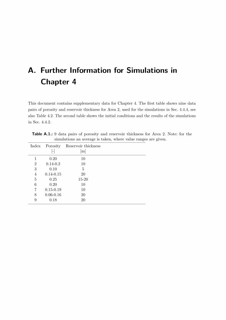
A. Further Information for Simulations inChapter 4
This document contains supplementary data for Chapter 4. The first table shows nine datapairs of porosity and reservoir thickness for Area 2, used for the simulations in Sec. 4.4.4, seealso Table 4.2. The second table shows the initial conditions and the results of the simulationsin Sec. 4.4.2.
Table A.1.: 9 data pairs of porosity and reservoir thickness for Area 2. Note: for thesimulations an average is taken, where value ranges are given.
Index Porosity Reservoir thickness[-] [m]
1 0.20 102 0.14-0.2 103 0.10 54 0.14-0.15 205 0.25 15-206 0.20 107 0.15-0.19 108 0.06-0.16 209 0.18 20
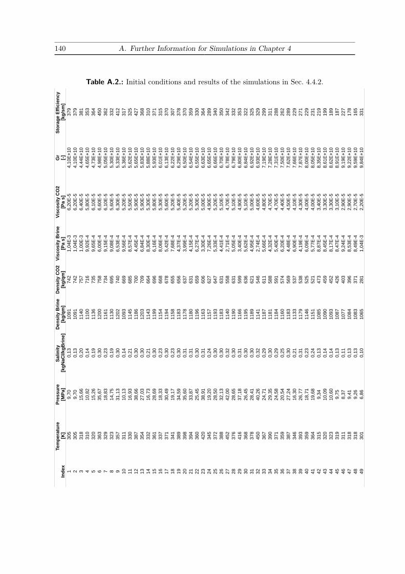
140 A. Further Information for Simulations in Chapter 4
Table A.2.: Initial conditions and results of the simulations in Sec. 4.4.2.
Ind
ex
1305
9,7
00,1
31091
742
1,0
4E-3
6,2
0E-5
4,1
0E+10
379
2305
9,7
00,1
31091
742
1,0
4E-3
6,2
0E-5
4,1
0E+10
379
3318
15,6
60,2
01140
757
1,0
0E-3
6,4
0E-5
4,4
4E+10
381
4310
10,8
20,1
41100
716
9,9
2E-4
5,8
0E-5
4,6
5E+10
353
5320
15,2
60,1
91136
735
9,6
5E-4
6,1
0E-5
4,7
3E+10
364
6363
35,6
70,3
01200
758
6,0
0E-4
6,6
0E-5
4,9
8E+10
450
7329
18,8
30,2
31161
734
9,1
5E-4
6,1
0E-5
5,0
5E+10
362
8323
14,7
50,1
91130
695
9,0
8E-4
5,6
0E-5
5,3
0E+10
332
9357
31,1
30,3
01202
740
6,5
3E-4
6,3
0E-5
5,3
3E+10
412
10
311
10,1
30,1
41093
669
9,5
6E-4
5,2
0E-5
5,3
6E+10
317
11
330
16,9
30,2
11145
685
8,5
7E-4
5,5
0E-5
5,6
2E+10
325
12
387
38,6
60,3
01186
700
4,4
5E-4
5,9
0E-5
5,6
5E+10
427
13
354
27,0
30,3
01203
709
6,8
4E-4
5,9
0E-5
5,8
3E+10
368
14
332
16,7
30,2
11143
664
8,3
0E-4
5,3
0E-5
5,8
8E+10
310
15
361
28,6
90,3
01199
696
6,1
6E-4
5,8
0E-5
5,9
3E+10
371
16
337
18,3
30,2
31154
668
8,0
6E-4
5,3
0E-5
6,0
1E+10
315
17
371
30,4
90,3
01194
678
5,4
2E-4
5,6
0E-5
6,1
3E+10
370
18
341
19,1
70,2
31158
655
7,6
8E-4
5,2
0E-5
6,2
2E+10
307
19
389
34,5
90,3
01183
656
4,3
7E-4
5,4
0E-5
6,2
9E+10
378
20
398
35,6
00,3
11178
637
3,9
9E-4
5,2
0E-5
6,5
0E+10
370
21
394
33,8
70,3
11180
631
4,1
5E-4
5,2
0E-5
6,5
4E+10
359
22
360
25,4
50,3
01196
659
6,2
7E-4
5,3
0E-5
6,5
5E+10
330
23
420
38,9
10,3
11163
606
3,3
0E-4
5,0
0E-5
6,6
3E+10
364
24
345
19,2
00,2
41157
627
7,2
6E-4
4,9
0E-5
6,6
5E+10
289
25
372
28,5
00,3
01193
647
5,3
3E-4
5,2
0E-5
6,6
6E+10
340
26
388
32,1
30,3
01183
631
4,4
1E-4
5,1
0E-5
6,7
0E+10
350
27
452
42,0
00,3
21140
558
2,7
1E-4
4,7
0E-5
6,7
8E+10
342
28
376
28,6
50,3
01190
631
5,0
5E-4
5,1
0E-5
6,7
9E+10
332
29
416
37,1
80,3
11166
599
3,4
0E-4
4,9
0E-5
6,8
0E+10
353
30
368
26,4
50,3
01195
636
5,6
2E-4
5,1
0E-5
6,8
4E+10
322
31
378
28,4
10,3
01189
621
4,9
5E-4
5,0
0E-5
6,9
2E+10
325
32
450
40,2
60,3
21141
546
2,7
4E-4
4,6
0E-5
6,9
3E+10
329
33
367
24,7
10,2
91187
611
5,6
6E-4
4,8
0E-5
7,1
9E+10
299
34
390
29,3
50,3
01181
588
4,3
2E-4
4,7
0E-5
7,2
8E+10
311
35
371
24,5
80,2
91184
591
5,4
0E-4
4,7
0E-5
7,3
1E+10
288
36
359
20,5
40,2
51160
574
6,2
0E-4
4,4
0E-5
7,5
0E+10
262
37
387
27,2
40,3
01183
569
4,4
8E-4
4,5
0E-5
7,6
2E+10
289
38
346
16,3
00,2
11133
537
6,9
0E-4
4,1
0E-5
7,6
6E+10
229
39
393
26,7
70,3
11179
538
4,1
9E-4
4,3
0E-5
7,8
7E+10
271
40
359
18,7
10,2
31146
525
6,0
9E-4
4,0
0E-5
8,0
0E+10
229
41
364
19,6
80,2
41151
521
5,7
7E-4
4,0
0E-5
8,0
5E+10
231
42
315
9,3
40,1
31085
473
8,8
7E-4
3,4
0E-5
8,3
5E+10
219
43
320
10,0
90,1
41090
459
8,4
5E-4
3,3
0E-5
8,6
1E+10
199
44
323
10,6
00,1
41093
452
8,1
7E-4
3,3
0E-5
8,6
2E+10
189
45
319
9,7
50,1
31087
426
8,4
7E-4
3,1
0E-5
8,9
1E+10
187
46
311
8,3
70,1
11077
403
9,2
4E-4
2,9
0E-5
9,1
9E+10
227
47
318
9,4
10,1
31084
396
8,5
3E-4
2,9
0E-5
9,2
2E+10
178
48
318
9,2
60,1
31083
371
8,4
9E-4
2,7
0E-5
9,5
9E+10
165
49
301
6,8
60,1
01065
281
1,0
4E-3
2,2
0E-5
9,8
4E+10
331
Tem
pe
ratu
re
[K]
Pre
ss
ure
[MP
a]
Sa
linit
y
[kg
Na
Cl/
kg
Bri
ne
]D
en
sit
y B
rin
e[k
g/q
m]
De
ns
ity
CO
2[k
g/q
m]
Vis
cos
ity
Bri
ne
[Pa
s]
Vis
co
sit
y C
O2
[Pa
s]
Gr
[-]
Sto
rag
e E
ffic
ien
cy
[kg
/sm
]


Institut für Wasser- und
Umweltsystemmodellierung
Universität Stuttgart
Pfaffenwaldring 61 70569 Stuttgart (Vaihingen) Telefon (0711) 685 - 64717/64749/64752/64679 Telefax (0711) 685 - 67020 o. 64746 o. 64681 E-Mail: [email protected] http://www.iws.uni-stuttgart.de
Direktoren Prof. Dr. rer. nat. Dr.-Ing. András Bárdossy Prof. Dr.-Ing. Rainer Helmig Prof. Dr.-Ing. Silke Wieprecht Prof. Dr.-Ing. Wolfgang Nowak
Vorstand (Stand 1.3.2016) Prof. Dr. rer. nat. Dr.-Ing. A. Bárdossy Prof. Dr.-Ing. R. Helmig Prof. Dr.-Ing. S. Wieprecht Prof. Dr. J.A. Sander Huisman Jürgen Braun, PhD apl. Prof. Dr.-Ing. H. Class Dr.-Ing. H.-P. Koschitzky Dr.-Ing. M. Noack Prof. Dr.-Ing. W. Nowak Dr. rer. nat. J. Seidel Dr.-Ing. K. Terheiden Dr.-Ing. habil. Sergey Oladyshkin
Emeriti Prof. Dr.-Ing. habil. Dr.-Ing. E.h. Jürgen Giesecke Prof. Dr.h.c. Dr.-Ing. E.h. Helmut Kobus, PhD
Lehrstuhl für Wasserbau und
Wassermengenwirtschaft Leiter: Prof. Dr.-Ing. Silke Wieprecht Stellv.: Dr.-Ing. Kristina Terheiden Versuchsanstalt für Wasserbau Leiter: Dr.-Ing. Markus Noack
Lehrstuhl für Hydromechanik
und Hydrosystemmodellierung Leiter: Prof. Dr.-Ing. Rainer Helmig Stellv.: apl. Prof. Dr.-Ing. Holger Class
Lehrstuhl für Hydrologie und Geohydrologie Leiter: Prof. Dr. rer. nat. Dr.-Ing. András Bárdossy Stellv.: Dr. rer. nat. Jochen Seidel Hydrogeophysik der Vadosen Zone (mit Forschungszentrum Jülich) Leiter: Prof. Dr. J.A. Sander Huisman
Lehrstuhl für Stochastische Simulation und
Sicherheitsforschung für Hydrosysteme Leiter: Prof. Dr.-Ing. Wolfgang Nowak Stellv.: Dr.-Ing. habil. Sergey Oladyshkin
VEGAS, Versuchseinrichtung zur
Grundwasser- und Altlastensanierung Leitung: Jürgen Braun, PhD, AD Dr.-Ing. Hans-Peter Koschitzky, AD
Verzeichnis der Mitteilungshefte
1 Röhnisch, Arthur: Die Bemühungen um eine Wasserbauliche Versuchsanstalt an
der Technischen Hochschule Stuttgart, und Fattah Abouleid, Abdel: Beitrag zur Berechnung einer in lockeren Sand geramm-ten, zweifach verankerten Spundwand, 1963
2 Marotz, Günter: Beitrag zur Frage der Standfestigkeit von dichten Asphaltbelägen
im Großwasserbau, 1964 3 Gurr, Siegfried: Beitrag zur Berechnung zusammengesetzter ebener Flächentrag-
werke unter besonderer Berücksichtigung ebener Stauwände, mit Hilfe von Rand-wert- und Lastwertmatrizen, 1965
4 Plica, Peter: Ein Beitrag zur Anwendung von Schalenkonstruktionen im Stahlwas-
serbau, und

2 Institut für Wasser- und Umweltsystemmodellierung * Universität Stuttgart * IWS
Petrikat, Kurt: Möglichkeiten und Grenzen des wasserbaulichen Versuchswesens, 1966
5 Plate, Erich: Beitrag zur Bestimmung der Windgeschwindigkeitsverteilung in der
durch eine Wand gestörten bodennahen Luftschicht, und Röhnisch, Arthur; Marotz, Günter: Neue Baustoffe und Bauausführungen für den Schutz der Böschungen und der Sohle von Kanälen, Flüssen und Häfen; Geste-hungskosten und jeweilige Vorteile, sowie Unny, T.E.: Schwingungsuntersuchungen am Kegelstrahlschieber, 1967
6 Seiler, Erich: Die Ermittlung des Anlagenwertes der bundeseigenen Bin-
nenschiffahrtsstraßen und Talsperren und des Anteils der Binnenschiffahrt an die-sem Wert, 1967
7 Sonderheft anläßlich des 65. Geburtstages von Prof. Arthur Röhnisch mit Beiträ-
gen von Benk, Dieter; Breitling, J.; Gurr, Siegfried; Haberhauer, Robert; Hone-kamp, Hermann; Kuz, Klaus Dieter; Marotz, Günter; Mayer-Vorfelder, Hans-Jörg; Miller, Rudolf; Plate, Erich J.; Radomski, Helge; Schwarz, Helmut; Vollmer, Ernst; Wildenhahn, Eberhard; 1967
8 Jumikis, Alfred: Beitrag zur experimentellen Untersuchung des Wassernach-
schubs in einem gefrierenden Boden und die Beurteilung der Ergebnisse, 1968 9 Marotz, Günter: Technische Grundlagen einer Wasserspeicherung im natürlichen
Untergrund, 1968 10 Radomski, Helge: Untersuchungen über den Einfluß der Querschnittsform wellen-
förmiger Spundwände auf die statischen und rammtechnischen Eigenschaften, 1968
11 Schwarz, Helmut: Die Grenztragfähigkeit des Baugrundes bei Einwirkung vertikal
gezogener Ankerplatten als zweidimensionales Bruchproblem, 1969 12 Erbel, Klaus: Ein Beitrag zur Untersuchung der Metamorphose von Mittelgebirgs-
schneedecken unter besonderer Berücksichtigung eines Verfahrens zur Bestim-mung der thermischen Schneequalität, 1969
13 Westhaus, Karl-Heinz: Der Strukturwandel in der Binnenschiffahrt und sein Einfluß
auf den Ausbau der Binnenschiffskanäle, 1969 14 Mayer-Vorfelder, Hans-Jörg: Ein Beitrag zur Berechnung des Erdwiderstandes un-
ter Ansatz der logarithmischen Spirale als Gleitflächenfunktion, 1970 15 Schulz, Manfred: Berechnung des räumlichen Erddruckes auf die Wandung kreis-
zylindrischer Körper, 1970 16 Mobasseri, Manoutschehr: Die Rippenstützmauer. Konstruktion und Grenzen ihrer
Standsicherheit, 1970 17 Benk, Dieter: Ein Beitrag zum Betrieb und zur Bemessung von Hochwasserrück-

Verzeichnis der Mitteilungshefte 3
haltebecken, 1970
18 Gàl, Attila: Bestimmung der mitschwingenden Wassermasse bei überströmten
Fischbauchklappen mit kreiszylindrischem Staublech, 1971, 19 Kuz, Klaus Dieter: Ein Beitrag zur Frage des Einsetzens von Kavitationserschei-
nungen in einer Düsenströmung bei Berücksichtigung der im Wasser gelösten Gase, 1971,
20 Schaak, Hartmut: Verteilleitungen von Wasserkraftanlagen, 1971 21 Sonderheft zur Eröffnung der neuen Versuchsanstalt des Instituts für Wasserbau
der Universität Stuttgart mit Beiträgen von Brombach, Hansjörg; Dirksen, Wolfram; Gàl, Attila; Gerlach, Reinhard; Giesecke, Jürgen; Holthoff, Franz-Josef; Kuz, Klaus Dieter; Marotz, Günter; Minor, Hans-Erwin; Petrikat, Kurt; Röhnisch, Arthur; Rueff, Helge; Schwarz, Helmut; Vollmer, Ernst; Wildenhahn, Eberhard; 1972
22 Wang, Chung-su: Ein Beitrag zur Berechnung der Schwingungen an Kegelstrahl-
schiebern, 1972 23 Mayer-Vorfelder, Hans-Jörg: Erdwiderstandsbeiwerte nach dem Ohde-
Variationsverfahren, 1972 24 Minor, Hans-Erwin: Beitrag zur Bestimmung der Schwingungsanfachungs-
funktionen überströmter Stauklappen, 1972, 25 Brombach, Hansjörg: Untersuchung strömungsmechanischer Elemente (Fluidik)
und die Möglichkeit der Anwendung von Wirbelkammerelementen im Wasserbau, 1972,
26 Wildenhahn, Eberhard: Beitrag zur Berechnung von Horizontalfilterbrunnen, 1972 27 Steinlein, Helmut: Die Eliminierung der Schwebstoffe aus Flußwasser zum Zweck
der unterirdischen Wasserspeicherung, gezeigt am Beispiel der Iller, 1972 28 Holthoff, Franz Josef: Die Überwindung großer Hubhöhen in der Binnenschiffahrt
durch Schwimmerhebewerke, 1973 29 Röder, Karl: Einwirkungen aus Baugrundbewegungen auf trog- und kastenförmige
Konstruktionen des Wasser- und Tunnelbaues, 1973 30 Kretschmer, Heinz: Die Bemessung von Bogenstaumauern in Abhängigkeit von
der Talform, 1973 31 Honekamp, Hermann: Beitrag zur Berechnung der Montage von Unterwasserpipe-
lines, 1973 32 Giesecke, Jürgen: Die Wirbelkammertriode als neuartiges Steuerorgan im Was-
serbau, und Brombach, Hansjörg: Entwicklung, Bauformen, Wirkungsweise und Steuereigen-schaften von Wirbelkammerverstärkern, 1974

4 Institut für Wasser- und Umweltsystemmodellierung * Universität Stuttgart * IWS 33 Rueff, Helge: Untersuchung der schwingungserregenden Kräfte an zwei hinterein-
ander angeordneten Tiefschützen unter besonderer Berücksichtigung von Kavita-tion, 1974
34 Röhnisch, Arthur: Einpreßversuche mit Zementmörtel für Spannbeton - Vergleich
der Ergebnisse von Modellversuchen mit Ausführungen in Hüllwellrohren, 1975 35 Sonderheft anläßlich des 65. Geburtstages von Prof. Dr.-Ing. Kurt Petrikat mit Bei-
trägen von: Brombach, Hansjörg; Erbel, Klaus; Flinspach, Dieter; Fischer jr., Richard; Gàl, Attila; Gerlach, Reinhard; Giesecke, Jürgen; Haberhauer, Robert; Hafner Edzard; Hausenblas, Bernhard; Horlacher, Hans-Burkhard; Hutarew, An-dreas; Knoll, Manfred; Krummet, Ralph; Marotz, Günter; Merkle, Theodor; Miller, Christoph; Minor, Hans-Erwin; Neumayer, Hans; Rao, Syamala; Rath, Paul; Rueff, Helge; Ruppert, Jürgen; Schwarz, Wolfgang; Topal-Gökceli, Mehmet; Vollmer, Ernst; Wang, Chung-su; Weber, Hans-Georg; 1975
36 Berger, Jochum: Beitrag zur Berechnung des Spannungszustandes in rotations-
symmetrisch belasteten Kugelschalen veränderlicher Wandstärke unter Gas- und Flüssigkeitsdruck durch Integration schwach singulärer Differentialgleichungen, 1975
37 Dirksen, Wolfram: Berechnung instationärer Abflußvorgänge in gestauten Gerin-
nen mittels Differenzenverfahren und die Anwendung auf Hochwasserrückhalte-becken, 1976
38 Horlacher, Hans-Burkhard: Berechnung instationärer Temperatur- und Wärme-
spannungsfelder in langen mehrschichtigen Hohlzylindern, 1976 39 Hafner, Edzard: Untersuchung der hydrodynamischen Kräfte auf Baukörper im
Tiefwasserbereich des Meeres, 1977, ISBN 3-921694-39-6 40 Ruppert, Jürgen: Über den Axialwirbelkammerverstärker für den Einsatz im Was-
serbau, 1977, ISBN 3-921694-40-X 41 Hutarew, Andreas: Beitrag zur Beeinflußbarkeit des Sauerstoffgehalts in Fließge-
wässern an Abstürzen und Wehren, 1977, ISBN 3-921694-41-8, 42 Miller, Christoph: Ein Beitrag zur Bestimmung der schwingungserregenden Kräfte
an unterströmten Wehren, 1977, ISBN 3-921694-42-6 43 Schwarz, Wolfgang: Druckstoßberechnung unter Berücksichtigung der Radial- und
Längsverschiebungen der Rohrwandung, 1978, ISBN 3-921694-43-4 44 Kinzelbach, Wolfgang: Numerische Untersuchungen über den optimalen Einsatz
variabler Kühlsysteme einer Kraftwerkskette am Beispiel Oberrhein, 1978, ISBN 3-921694-44-2
45 Barczewski, Baldur: Neue Meßmethoden für Wasser-Luftgemische und deren An-
wendung auf zweiphasige Auftriebsstrahlen, 1979, ISBN 3-921694-45-0

Verzeichnis der Mitteilungshefte 5
46 Neumayer, Hans: Untersuchung der Strömungsvorgänge in radialen Wirbelkam-
merverstärkern, 1979, ISBN 3-921694-46-9 47 Elalfy, Youssef-Elhassan: Untersuchung der Strömungsvorgänge in Wirbelkam-
merdioden und -drosseln, 1979, ISBN 3-921694-47-7 48 Brombach, Hansjörg: Automatisierung der Bewirtschaftung von Wasserspeichern,
1981, ISBN 3-921694-48-5 49 Geldner, Peter: Deterministische und stochastische Methoden zur Bestimmung
der Selbstdichtung von Gewässern, 1981, ISBN 3-921694-49-3, 50 Mehlhorn, Hans: Temperaturveränderungen im Grundwasser durch Brauchwas-
sereinleitungen, 1982, ISBN 3-921694-50-7, 51 Hafner, Edzard: Rohrleitungen und Behälter im Meer, 1983, ISBN 3-921694-51-5 52 Rinnert, Bernd: Hydrodynamische Dispersion in porösen Medien: Einfluß von
Dichteunterschieden auf die Vertikalvermischung in horizontaler Strömung, 1983, ISBN 3-921694-52-3,
53 Lindner, Wulf: Steuerung von Grundwasserentnahmen unter Einhaltung ökologi-
scher Kriterien, 1983, ISBN 3-921694-53-1, 54 Herr, Michael; Herzer, Jörg; Kinzelbach, Wolfgang; Kobus, Helmut; Rinnert,
Bernd: Methoden zur rechnerischen Erfassung und hydraulischen Sanierung von Grundwasserkontaminationen, 1983, ISBN 3-921694-54-X
55 Schmitt, Paul: Wege zur Automatisierung der Niederschlagsermittlung, 1984,
ISBN 3-921694-55-8, 56 Müller, Peter: Transport und selektive Sedimentation von Schwebstoffen bei ge-
stautem Abfluß, 1985, ISBN 3-921694-56-6 57 El-Qawasmeh, Fuad: Möglichkeiten und Grenzen der Tropfbewässerung unter be-
sonderer Berücksichtigung der Verstopfungsanfälligkeit der Tropfelemente, 1985, ISBN 3-921694-57-4,
58 Kirchenbaur, Klaus: Mikroprozessorgesteuerte Erfassung instationärer Druckfelder
am Beispiel seegangsbelasteter Baukörper, 1985, ISBN 3-921694-58-2 59 Kobus, Helmut (Hrsg.): Modellierung des großräumigen Wärme- und Schadstoff-
transports im Grundwasser, Tätigkeitsbericht 1984/85 (DFG-Forschergruppe an den Universitäten Hohenheim, Karlsruhe und Stuttgart), 1985, ISBN 3-921694-59-0,
60 Spitz, Karlheinz: Dispersion in porösen Medien: Einfluß von Inhomogenitäten und
Dichteunterschieden, 1985, ISBN 3-921694-60-4, 61 Kobus, Helmut: An Introduction to Air-Water Flows in Hydraulics, 1985,
ISBN 3-921694-61-2
6 Institut für Wasser- und Umweltsystemmodellierung * Universität Stuttgart * IWS 62 Kaleris, Vassilios: Erfassung des Austausches von Oberflächen- und Grundwas-
ser in horizontalebenen Grundwassermodellen, 1986, ISBN 3-921694-62-0 63 Herr, Michael: Grundlagen der hydraulischen Sanierung verunreinigter Poren-
grundwasserleiter, 1987, ISBN 3-921694-63-9 64 Marx, Walter: Berechnung von Temperatur und Spannung in Massenbeton infolge
Hydratation, 1987, ISBN 3-921694-64-7 65 Koschitzky, Hans-Peter: Dimensionierungskonzept für Sohlbelüfter in Schußrinnen
zur Vermeidung von Kavitationsschäden, 1987, ISBN 3-921694-65-5 66 Kobus, Helmut (Hrsg.): Modellierung des großräumigen Wärme- und Schadstoff-
transports im Grundwasser, Tätigkeitsbericht 1986/87 (DFG-Forschergruppe an den Universitäten Hohenheim, Karlsruhe und Stuttgart) 1987, ISBN 3-921694-66-3
67 Söll, Thomas: Berechnungsverfahren zur Abschätzung anthropogener Tempera-
turanomalien im Grundwasser, 1988, ISBN 3-921694-67-1 68 Dittrich, Andreas; Westrich, Bernd: Bodenseeufererosion, Bestandsaufnahme und
Bewertung, 1988, ISBN 3-921694-68-X, 69 Huwe, Bernd; van der Ploeg, Rienk R.: Modelle zur Simulation des Stickstoffhaus-
haltes von Standorten mit unterschiedlicher landwirtschaftlicher Nutzung, 1988, ISBN 3-921694-69-8,
70 Stephan, Karl: Integration elliptischer Funktionen, 1988, ISBN 3-921694-70-1 71 Kobus, Helmut; Zilliox, Lothaire (Hrsg.): Nitratbelastung des Grundwassers, Aus-
wirkungen der Landwirtschaft auf die Grundwasser- und Rohwasserbeschaf-fenheit und Maßnahmen zum Schutz des Grundwassers. Vorträge des deutsch-französischen Kolloquiums am 6. Oktober 1988, Universitäten Stuttgart und Louis Pasteur Strasbourg (Vorträge in deutsch oder französisch, Kurzfassungen zwei-sprachig), 1988, ISBN 3-921694-71-X
72 Soyeaux, Renald: Unterströmung von Stauanlagen auf klüftigem Untergrund unter
Berücksichtigung laminarer und turbulenter Fließzustände,1991, ISBN 3-921694-72-8
73 Kohane, Roberto: Berechnungsmethoden für Hochwasserabfluß in Fließgewäs-
sern mit überströmten Vorländern, 1991, ISBN 3-921694-73-6 74 Hassinger, Reinhard: Beitrag zur Hydraulik und Bemessung von Blocksteinrampen
in flexibler Bauweise, 1991, ISBN 3-921694-74-4, 75 Schäfer, Gerhard: Einfluß von Schichtenstrukturen und lokalen Einlagerungen auf
die Längsdispersion in Porengrundwasserleitern, 1991, ISBN 3-921694-75-2 76 Giesecke, Jürgen: Vorträge, Wasserwirtschaft in stark besiedelten Regionen; Um-
weltforschung mit Schwerpunkt Wasserwirtschaft, 1991, ISBN 3-921694-76-0
Verzeichnis der Mitteilungshefte 7
77 Huwe, Bernd: Deterministische und stochastische Ansätze zur Modellierung des
Stickstoffhaushalts landwirtschaftlich genutzter Flächen auf unterschiedlichem Skalenniveau, 1992, ISBN 3-921694-77-9,
78 Rommel, Michael: Verwendung von Kluftdaten zur realitätsnahen Generierung von
Kluftnetzen mit anschließender laminar-turbulenter Strömungsberechnung, 1993, ISBN 3-92 1694-78-7
79 Marschall, Paul: Die Ermittlung lokaler Stofffrachten im Grundwasser mit Hilfe von
Einbohrloch-Meßverfahren, 1993, ISBN 3-921694-79-5, 80 Ptak, Thomas: Stofftransport in heterogenen Porenaquiferen: Felduntersuchungen
und stochastische Modellierung, 1993, ISBN 3-921694-80-9, 81 Haakh, Frieder: Transientes Strömungsverhalten in Wirbelkammern, 1993,
ISBN 3-921694-81-7 82 Kobus, Helmut; Cirpka, Olaf; Barczewski, Baldur; Koschitzky, Hans-Peter: Ver-
sucheinrichtung zur Grundwasser und Altlastensanierung VEGAS, Konzeption und Programmrahmen, 1993, ISBN 3-921694-82-5
83 Zang, Weidong: Optimaler Echtzeit-Betrieb eines Speichers mit aktueller Abflußre-
generierung, 1994, ISBN 3-921694-83-3, 84 Franke, Hans-Jörg: Stochastische Modellierung eines flächenhaften Stoffeintrages
und Transports in Grundwasser am Beispiel der Pflanzenschutzmittelproblematik, 1995, ISBN 3-921694-84-1
85 Lang, Ulrich: Simulation regionaler Strömungs- und Transportvorgänge in Karst-
aquiferen mit Hilfe des Doppelkontinuum-Ansatzes: Methodenentwicklung und Pa-rameteridentifikation, 1995, ISBN 3-921694-85-X,
86 Helmig, Rainer: Einführung in die Numerischen Methoden der Hydromechanik,
1996, ISBN 3-921694-86-8, 87 Cirpka, Olaf: CONTRACT: A Numerical Tool for Contaminant Transport and
Chemical Transformations - Theory and Program Documentation -, 1996, ISBN 3-921694-87-6
88 Haberlandt, Uwe: Stochastische Synthese und Regionalisierung des Niederschla-
ges für Schmutzfrachtberechnungen, 1996, ISBN 3-921694-88-4 89 Croisé, Jean: Extraktion von flüchtigen Chemikalien aus natürlichen Lockergestei-
nen mittels erzwungener Luftströmung, 1996, ISBN 3-921694-89-2, 90 Jorde, Klaus: Ökologisch begründete, dynamische Mindestwasserregelungen bei
Ausleitungskraftwerken, 1997, ISBN 3-921694-90-6, 91 Helmig, Rainer: Gekoppelte Strömungs- und Transportprozesse im Untergrund -
Ein Beitrag zur Hydrosystemmodellierung-, 1998, ISBN 3-921694-91-4,

8 Institut für Wasser- und Umweltsystemmodellierung * Universität Stuttgart * IWS 92 Emmert, Martin: Numerische Modellierung nichtisothermer Gas-Wasser Systeme
in porösen Medien, 1997, ISBN 3-921694-92-2 93 Kern, Ulrich: Transport von Schweb- und Schadstoffen in staugeregelten Fließge-
wässern am Beispiel des Neckars, 1997, ISBN 3-921694-93-0, 94 Förster, Georg: Druckstoßdämpfung durch große Luftblasen in Hochpunkten von
Rohrleitungen 1997, ISBN 3-921694-94-9 95 Cirpka, Olaf: Numerische Methoden zur Simulation des reaktiven Mehrkomponen-
tentransports im Grundwasser, 1997, ISBN 3-921694-95-7, 96 Färber, Arne: Wärmetransport in der ungesättigten Bodenzone: Entwicklung einer
thermischen In-situ-Sanierungstechnologie, 1997, ISBN 3-921694-96-5 97 Betz, Christoph: Wasserdampfdestillation von Schadstoffen im porösen Medium:
Entwicklung einer thermischen In-situ-Sanierungstechnologie, 1998, ISBN 3-921694-97-3
98 Xu, Yichun: Numerical Modeling of Suspended Sediment Transport in Rivers,
1998, ISBN 3-921694-98-1, 99 Wüst, Wolfgang: Geochemische Untersuchungen zur Sanierung CKW-
kontaminierter Aquifere mit Fe(0)-Reaktionswänden, 2000, ISBN 3-933761-02-2 100 Sheta, Hussam: Simulation von Mehrphasenvorgängen in porösen Medien unter
Einbeziehung von Hysterese-Effekten, 2000, ISBN 3-933761-03-4 101 Ayros, Edwin: Regionalisierung extremer Abflüsse auf der Grundlage statistischer
Verfahren, 2000, ISBN 3-933761-04-2, 102 Huber, Ralf: Compositional Multiphase Flow and Transport in Heterogeneous Po-
rous Media, 2000, ISBN 3-933761-05-0 103 Braun, Christopherus: Ein Upscaling-Verfahren für Mehrphasenströmungen in po-
rösen Medien, 2000, ISBN 3-933761-06-9 104 Hofmann, Bernd: Entwicklung eines rechnergestützten Managementsystems zur
Beurteilung von Grundwasserschadensfällen, 2000, ISBN 3-933761-07-7 105 Class, Holger: Theorie und numerische Modellierung nichtisothermer Mehrphasen-
prozesse in NAPL-kontaminierten porösen Medien, 2001, ISBN 3-933761-08-5
106 Schmidt, Reinhard: Wasserdampf- und Heißluftinjektion zur thermischen Sanie-
rung kontaminierter Standorte, 2001, ISBN 3-933761-09-3 107 Josef, Reinhold:, Schadstoffextraktion mit hydraulischen Sanierungsverfahren un-
ter Anwendung von grenzflächenaktiven Stoffen, 2001, ISBN 3-933761-10-7
Verzeichnis der Mitteilungshefte 9
108 Schneider, Matthias: Habitat- und Abflussmodellierung für Fließgewässer mit un-
scharfen Berechnungsansätzen, 2001, ISBN 3-933761-11-5 109 Rathgeb, Andreas: Hydrodynamische Bemessungsgrundlagen für Lockerdeck-
werke an überströmbaren Erddämmen, 2001, ISBN 3-933761-12-3 110 Lang, Stefan: Parallele numerische Simulation instätionärer Probleme mit adapti-
ven Methoden auf unstrukturierten Gittern, 2001, ISBN 3-933761-13-1 111 Appt, Jochen; Stumpp Simone: Die Bodensee-Messkampagne 2001, IWS/CWR
Lake Constance Measurement Program 2001, 2002, ISBN 3-933761-14-X 112 Heimerl, Stephan: Systematische Beurteilung von Wasserkraftprojekten, 2002,
ISBN 3-933761-15-8, 113 Iqbal, Amin: On the Management and Salinity Control of Drip Irrigation, 2002, ISBN
3-933761-16-6 114 Silberhorn-Hemminger, Annette: Modellierung von Kluftaquifersystemen: Geosta-
tistische Analyse und deterministisch-stochastische Kluftgenerierung, 2002, ISBN 3-933761-17-4
115 Winkler, Angela: Prozesse des Wärme- und Stofftransports bei der In-situ-
Sanierung mit festen Wärmequellen, 2003, ISBN 3-933761-18-2 116 Marx, Walter: Wasserkraft, Bewässerung, Umwelt - Planungs- und Bewertungs-
schwerpunkte der Wasserbewirtschaftung, 2003, ISBN 3-933761-19-0 117 Hinkelmann, Reinhard: Efficient Numerical Methods and Information-Processing
Techniques in Environment Water, 2003, ISBN 3-933761-20-4 118 Samaniego-Eguiguren, Luis Eduardo: Hydrological Consequences of Land Use /
Land Cover and Climatic Changes in Mesoscale Catchments, 2003, ISBN 3-933761-21-2
119 Neunhäuserer, Lina: Diskretisierungsansätze zur Modellierung von Strömungs-
und Transportprozessen in geklüftet-porösen Medien, 2003, ISBN 3-933761-22-0 120 Paul, Maren: Simulation of Two-Phase Flow in Heterogeneous Poros Media with
Adaptive Methods, 2003, ISBN 3-933761-23-9 121 Ehret, Uwe: Rainfall and Flood Nowcasting in Small Catchments using Weather
Radar, 2003, ISBN 3-933761-24-7 122 Haag, Ingo: Der Sauerstoffhaushalt staugeregelter Flüsse am Beispiel des
Neckars - Analysen, Experimente, Simulationen -, 2003, ISBN 3-933761-25-5 123 Appt, Jochen: Analysis of Basin-Scale Internal Waves in Upper Lake Constance,
2003, ISBN 3-933761-26-3
10 Institut für Wasser- und Umweltsystemmodellierung * Universität Stuttgart * IWS 124 Hrsg.: Schrenk, Volker; Batereau, Katrin; Barczewski, Baldur; Weber, Karolin und
Koschitzky, Hans-Peter: Symposium Ressource Fläche und VEGAS - Statuskol-loquium 2003, 30. September und 1. Oktober 2003, 2003, ISBN 3-933761-27-1
125 Omar Khalil Ouda: Optimisation of Agricultural Water Use: A Decision Support
System for the Gaza Strip, 2003, ISBN 3-933761-28-0 126 Batereau, Katrin: Sensorbasierte Bodenluftmessung zur Vor-Ort-Erkundung von
Schadensherden im Untergrund, 2004, ISBN 3-933761-29-8 127 Witt, Oliver: Erosionsstabilität von Gewässersedimenten mit Auswirkung auf den
Stofftransport bei Hochwasser am Beispiel ausgewählter Stauhaltungen des Ober-rheins, 2004, ISBN 3-933761-30-1
128 Jakobs, Hartmut: Simulation nicht-isothermer Gas-Wasser-Prozesse in komplexen
Kluft-Matrix-Systemen, 2004, ISBN 3-933761-31-X 129 Li, Chen-Chien: Deterministisch-stochastisches Berechnungskonzept zur Beurtei-
lung der Auswirkungen erosiver Hochwasserereignisse in Flussstauhaltungen, 2004, ISBN 3-933761-32-8
130 Reichenberger, Volker; Helmig, Rainer; Jakobs, Hartmut; Bastian, Peter; Niessner,
Jennifer: Complex Gas-Water Processes in Discrete Fracture-Matrix Systems: Up-scaling, Mass-Conservative Discretization and Efficient Multilevel Solution, 2004, ISBN 3-933761-33-6
131 Hrsg.: Barczewski, Baldur; Koschitzky, Hans-Peter; Weber, Karolin; Wege, Ralf:
VEGAS - Statuskolloquium 2004, Tagungsband zur Veranstaltung am 05. Oktober 2004 an der Universität Stuttgart, Campus Stuttgart-Vaihingen, 2004, ISBN 3-933761-34-4
132 Asie, Kemal Jabir: Finite Volume Models for Multiphase Multicomponent Flow
through Porous Media. 2005, ISBN 3-933761-35-2 133 Jacoub, George: Development of a 2-D Numerical Module for Particulate Contam-
inant Transport in Flood Retention Reservoirs and Impounded Rivers, 2004, ISBN 3-933761-36-0
134 Nowak, Wolfgang: Geostatistical Methods for the Identification of Flow and
Transport Parameters in the Subsurface, 2005, ISBN 3-933761-37-9 135 Süß, Mia: Analysis of the influence of structures and boundaries on flow and
transport processes in fractured porous media, 2005, ISBN 3-933761-38-7 136 Jose, Surabhin Chackiath: Experimental Investigations on Longitudinal Dispersive
Mixing in Heterogeneous Aquifers, 2005, ISBN: 3-933761-39-5 137 Filiz, Fulya: Linking Large-Scale Meteorological Conditions to Floods in Mesoscale
Catchments, 2005, ISBN 3-933761-40-9
Verzeichnis der Mitteilungshefte 11
138 Qin, Minghao: Wirklichkeitsnahe und recheneffiziente Ermittlung von Temperatur
und Spannungen bei großen RCC-Staumauern, 2005, ISBN 3-933761-41-7 139 Kobayashi, Kenichiro: Optimization Methods for Multiphase Systems in the Sub-
surface - Application to Methane Migration in Coal Mining Areas, 2005, ISBN 3-933761-42-5
140 Rahman, Md. Arifur: Experimental Investigations on Transverse Dispersive Mixing
in Heterogeneous Porous Media, 2005, ISBN 3-933761-43-3 141 Schrenk, Volker: Ökobilanzen zur Bewertung von Altlastensanierungsmaßnah-
men, 2005, ISBN 3-933761-44-1 142 Hundecha, Hirpa Yeshewatesfa: Regionalization of Parameters of a Conceptual
Rainfall-Runoff Model, 2005, ISBN: 3-933761-45-X 143 Wege, Ralf: Untersuchungs- und Überwachungsmethoden für die Beurteilung na-
türlicher Selbstreinigungsprozesse im Grundwasser, 2005, ISBN 3-933761-46-8 144 Breiting, Thomas: Techniken und Methoden der Hydroinformatik - Modellierung
von komplexen Hydrosystemen im Untergrund, 2006, 3-933761-47-6 145 Hrsg.: Braun, Jürgen; Koschitzky, Hans-Peter; Müller, Martin: Ressource Unter-
grund: 10 Jahre VEGAS: Forschung und Technologieentwicklung zum Schutz von Grundwasser und Boden, Tagungsband zur Veranstaltung am 28. und 29. Sep-tember 2005 an der Universität Stuttgart, Campus Stuttgart-Vaihingen, 2005, ISBN 3-933761-48-4
146 Rojanschi, Vlad: Abflusskonzentration in mesoskaligen Einzugsgebieten unter
Berücksichtigung des Sickerraumes, 2006, ISBN 3-933761-49-2 147 Winkler, Nina Simone: Optimierung der Steuerung von Hochwasserrückhaltebe-
cken-systemen, 2006, ISBN 3-933761-50-6 148 Wolf, Jens: Räumlich differenzierte Modellierung der Grundwasserströmung allu-
vialer Aquifere für mesoskalige Einzugsgebiete, 2006, ISBN: 3-933761-51-4 149 Kohler, Beate: Externe Effekte der Laufwasserkraftnutzung, 2006,
ISBN 3-933761-52-2 150 Hrsg.: Braun, Jürgen; Koschitzky, Hans-Peter; Stuhrmann, Matthias: VEGAS-
Statuskolloquium 2006, Tagungsband zur Veranstaltung am 28. September 2006 an der Universität Stuttgart, Campus Stuttgart-Vaihingen, 2006, ISBN 3-933761-53-0
151 Niessner, Jennifer: Multi-Scale Modeling of Multi-Phase - Multi-Component Pro-
cesses in Heterogeneous Porous Media, 2006, ISBN 3-933761-54-9 152 Fischer, Markus: Beanspruchung eingeerdeter Rohrleitungen infolge Austrock-
nung bindiger Böden, 2006, ISBN 3-933761-55-7

12 Institut für Wasser- und Umweltsystemmodellierung * Universität Stuttgart * IWS 153 Schneck, Alexander: Optimierung der Grundwasserbewirtschaftung unter Berück-
sichtigung der Belange der Wasserversorgung, der Landwirtschaft und des Natur-schutzes, 2006, ISBN 3-933761-56-5
154 Das, Tapash: The Impact of Spatial Variability of Precipitation on the Predictive
Uncertainty of Hydrological Models, 2006, ISBN 3-933761-57-3 155 Bielinski, Andreas: Numerical Simulation of CO2 sequestration in geological for-
mations, 2007, ISBN 3-933761-58-1 156 Mödinger, Jens: Entwicklung eines Bewertungs- und Entscheidungsunterstüt-
zungssystems für eine nachhaltige regionale Grundwasserbewirtschaftung, 2006, ISBN 3-933761-60-3
157 Manthey, Sabine: Two-phase flow processes with dynamic effects in porous
media - parameter estimation and simulation, 2007, ISBN 3-933761-61-1 158 Pozos Estrada, Oscar: Investigation on the Effects of Entrained Air in Pipelines,
2007, ISBN 3-933761-62-X 159 Ochs, Steffen Oliver: Steam injection into saturated porous media – process anal-
ysis including experimental and numerical investigations, 2007, ISBN 3-933761-63-8
160 Marx, Andreas: Einsatz gekoppelter Modelle und Wetterradar zur Abschätzung
von Niederschlagsintensitäten und zur Abflussvorhersage, 2007, ISBN 3-933761-64-6
161 Hartmann, Gabriele Maria: Investigation of Evapotranspiration Concepts in Hydro-
logical Modelling for Climate Change Impact Assessment, 2007, ISBN 3-933761-65-4
162 Kebede Gurmessa, Tesfaye: Numerical Investigation on Flow and Transport
Characteristics to Improve Long-Term Simulation of Reservoir Sedimentation, 2007, ISBN 3-933761-66-2
163 Trifković, Aleksandar: Multi-objective and Risk-based Modelling Methodology for
Planning, Design and Operation of Water Supply Systems, 2007, ISBN 3-933761-67-0
164 Götzinger, Jens: Distributed Conceptual Hydrological Modelling - Simulation of
Climate, Land Use Change Impact and Uncertainty Analysis, 2007, ISBN 3-933761-68-9
165 Hrsg.: Braun, Jürgen; Koschitzky, Hans-Peter; Stuhrmann, Matthias: VEGAS –
Kolloquium 2007, Tagungsband zur Veranstaltung am 26. September 2007 an der Universität Stuttgart, Campus Stuttgart-Vaihingen, 2007, ISBN 3-933761-69-7
166 Freeman, Beau: Modernization Criteria Assessment for Water Resources Plan-
ning; Klamath Irrigation Project, U.S., 2008, ISBN 3-933761-70-0
Verzeichnis der Mitteilungshefte 13
167 Dreher, Thomas: Selektive Sedimentation von Feinstschwebstoffen in Wechsel-
wirkung mit wandnahen turbulenten Strömungsbedingungen, 2008, ISBN 3-933761-71-9
168 Yang, Wei: Discrete-Continuous Downscaling Model for Generating Daily Precipi-
tation Time Series, 2008, ISBN 3-933761-72-7 169 Kopecki, Ianina: Calculational Approach to FST-Hemispheres for Multiparametrical
Benthos Habitat Modelling, 2008, ISBN 3-933761-73-5 170 Brommundt, Jürgen: Stochastische Generierung räumlich zusammenhängender
Niederschlagszeitreihen, 2008, ISBN 3-933761-74-3 171 Papafotiou, Alexandros: Numerical Investigations of the Role of Hysteresis in Het-
erogeneous Two-Phase Flow Systems, 2008, ISBN 3-933761-75-1 172 He, Yi: Application of a Non-Parametric Classification Scheme to Catchment Hy-
drology, 2008, ISBN 978-3-933761-76-7 173 Wagner, Sven: Water Balance in a Poorly Gauged Basin in West Africa Using At-
mospheric Modelling and Remote Sensing Information, 2008, ISBN 978-3-933761-77-4
174 Hrsg.: Braun, Jürgen; Koschitzky, Hans-Peter; Stuhrmann, Matthias; Schrenk,
Volker: VEGAS-Kolloquium 2008 Ressource Fläche III, Tagungsband zur Veran-staltung am 01. Oktober 2008 an der Universität Stuttgart, Campus Stuttgart-Vaihingen, 2008, ISBN 978-3-933761-78-1
175 Patil, Sachin: Regionalization of an Event Based Nash Cascade Model for Flood
Predictions in Ungauged Basins, 2008, ISBN 978-3-933761-79-8 176 Assteerawatt, Anongnart: Flow and Transport Modelling of Fractured Aquifers
based on a Geostatistical Approach, 2008, ISBN 978-3-933761-80-4 177 Karnahl, Joachim Alexander: 2D numerische Modellierung von multifraktionalem
Schwebstoff- und Schadstofftransport in Flüssen, 2008, ISBN 978-3-933761-81-1 178 Hiester, Uwe: Technologieentwicklung zur In-situ-Sanierung der ungesättigten Bo-
denzone mit festen Wärmequellen, 2009, ISBN 978-3-933761-82-8 179 Laux, Patrick: Statistical Modeling of Precipitation for Agricultural Planning in the
Volta Basin of West Africa, 2009, ISBN 978-3-933761-83-5 180 Ehsan, Saqib: Evaluation of Life Safety Risks Related to Severe Flooding, 2009,
ISBN 978-3-933761-84-2 181 Prohaska, Sandra: Development and Application of a 1D Multi-Strip Fine Sedi-
ment Transport Model for Regulated Rivers, 2009, ISBN 978-3-933761-85-9

14 Institut für Wasser- und Umweltsystemmodellierung * Universität Stuttgart * IWS 182 Kopp, Andreas: Evaluation of CO2 Injection Processes in Geological Formations
for Site Screening, 2009, ISBN 978-3-933761-86-6 183 Ebigbo, Anozie: Modelling of biofilm growth and its influence on CO2 and water
(two-phase) flow in porous media, 2009, ISBN 978-3-933761-87-3 184 Freiboth, Sandra: A phenomenological model for the numerical simulation of
multiphase multicomponent processes considering structural alterations of po-rous media, 2009, ISBN 978-3-933761-88-0
185 Zöllner, Frank: Implementierung und Anwendung netzfreier Methoden im Kon-
struktiven Wasserbau und in der Hydromechanik, 2009, ISBN 978-3-933761-89-7
186 Vasin, Milos: Influence of the soil structure and property contrast on flow and
transport in the unsaturated zone, 2010, ISBN 978-3-933761-90-3 187 Li, Jing: Application of Copulas as a New Geostatistical Tool, 2010, ISBN 978-3-
933761-91-0 188 AghaKouchak, Amir: Simulation of Remotely Sensed Rainfall Fields Using Copu-
las, 2010, ISBN 978-3-933761-92-7 189 Thapa, Pawan Kumar: Physically-based spatially distributed rainfall runoff model-
ling for soil erosion estimation, 2010, ISBN 978-3-933761-93-4 190 Wurms, Sven: Numerische Modellierung der Sedimentationsprozesse in Retenti-
onsanlagen zur Steuerung von Stoffströmen bei extremen Hochwasserabflusser-eignissen, 2011, ISBN 978-3-933761-94-1
191 Merkel, Uwe: Unsicherheitsanalyse hydraulischer Einwirkungen auf Hochwasser-
schutzdeiche und Steigerung der Leistungsfähigkeit durch adaptive Strömungs-modellierung, 2011, ISBN 978-3-933761-95-8
192 Fritz, Jochen: A Decoupled Model for Compositional Non-Isothermal Multiphase
Flow in Porous Media and Multiphysics Approaches for Two-Phase Flow, 2010, ISBN 978-3-933761-96-5
193 Weber, Karolin (Hrsg.): 12. Treffen junger WissenschaftlerInnen an Wasserbauin-
stituten, 2010, ISBN 978-3-933761-97-2 194 Bliefernicht, Jan-Geert: Probability Forecasts of Daily Areal Precipitation for Small
River Basins, 2011, ISBN 978-3-933761-98-9 195 Hrsg.: Koschitzky, Hans-Peter; Braun, Jürgen: VEGAS-Kolloquium 2010 In-situ-
Sanierung - Stand und Entwicklung Nano und ISCO -, Tagungsband zur Veran-staltung am 07. Oktober 2010 an der Universität Stuttgart, Campus Stuttgart-Vaihingen, 2010, ISBN 978-3-933761-99-6
Verzeichnis der Mitteilungshefte 15
196 Gafurov, Abror: Water Balance Modeling Using Remote Sensing Information - Fo-
cus on Central Asia, 2010, ISBN 978-3-942036-00-9 197 Mackenberg, Sylvia: Die Quellstärke in der Sickerwasserprognose:
Möglichkeiten und Grenzen von Labor- und Freilanduntersuchungen, 2010, ISBN 978-3-942036-01-6
198 Singh, Shailesh Kumar: Robust Parameter Estimation in Gauged and Ungauged
Basins, 2010, ISBN 978-3-942036-02-3 199 Doğan, Mehmet Onur: Coupling of porous media flow with pipe flow, 2011,
ISBN 978-3-942036-03-0 200 Liu, Min: Study of Topographic Effects on Hydrological Patterns and the Implica-
tion on Hydrological Modeling and Data Interpolation, 2011, ISBN 978-3-942036-04-7
201 Geleta, Habtamu Itefa: Watershed Sediment Yield Modeling for Data Scarce Are-
as, 2011, ISBN 978-3-942036-05-4 202 Franke, Jörg: Einfluss der Überwachung auf die Versagenswahrscheinlichkeit von
Staustufen, 2011, ISBN 978-3-942036-06-1 203 Bakimchandra, Oinam: Integrated Fuzzy-GIS approach for assessing regional soil
erosion risks, 2011, ISBN 978-3-942036-07-8 204 Alam, Muhammad Mahboob: Statistical Downscaling of Extremes of Precipita-
tion in Mesoscale Catchments from Different RCMs and Their Effects on Local Hydrology, 2011, ISBN 978-3-942036-08-5
205 Hrsg.: Koschitzky, Hans-Peter; Braun, Jürgen: VEGAS-Kolloquium 2011 Flache
Geothermie - Perspektiven und Risiken, Tagungsband zur Veranstaltung am 06. Oktober 2011 an der Universität Stuttgart, Campus Stuttgart-Vaihingen, 2011, ISBN 978-3-933761-09-2
206 Haslauer, Claus: Analysis of Real-World Spatial Dependence of Subsurface
Hydraulic Properties Using Copulas with a Focus on Solute Transport Behav-iour, 2011, ISBN 978-3-942036-10-8
207 Dung, Nguyen Viet: Multi-objective automatic calibration of hydrodynamic mod-
els – development of the concept and an application in the Mekong Delta, 2011, ISBN 978-3-942036-11-5
208 Hung, Nguyen Nghia: Sediment dynamics in the floodplain of the
Mekong Delta, Vietnam, 2011, ISBN 978-3-942036-12-2 209 Kuhlmann, Anna: Influence of soil structure and root water uptake on flow in
the unsaturated zone, 2012, ISBN 978-3-942036-13-9

16 Institut für Wasser- und Umweltsystemmodellierung * Universität Stuttgart * IWS 210 Tuhtan, Jeffrey Andrew: Including the Second Law Inequality in Aquatic Ecody-
namics: A Modeling Approach for Alpine Rivers Impacted by Hydropeaking, 2012, ISBN 978-3-942036-14-6
211 Tolossa, Habtamu: Sediment Transport Computation Using a Data-Driven Adap-
tive Neuro-Fuzzy Modelling Approach, 2012, ISBN 978-3-942036-15-3 212 Tatomir, Alexandru-Bodgan: From Discrete to Continuum Concepts of Flow in
Fractured Porous Media, 2012, ISBN 978-3-942036-16-0 213 Erbertseder, Karin: A Multi-Scale Model for Describing Cancer-Therapeutic
Transport in the Human Lung, 2012, ISBN 978-3-942036-17-7 214 Noack, Markus: Modelling Approach for Interstitial Sediment Dynamics and Re-
production of Gravel Spawning Fish, 2012, ISBN 978-3-942036-18-4 215 De Boer, Cjestmir Volkert: Transport of Nano Sized Zero Valent Iron Colloids dur-
ing Injection into the Subsurface, 2012, ISBN 978-3-942036-19-1 216 Pfaff, Thomas: Processing and Analysis of Weather Radar Data for Use in Hydro-
logy, 2013, ISBN 978-3-942036-20-7 217 Lebrenz, Hans-Henning: Addressing the Input Uncertainty for Hydrological Model-
ing by a New Geostatistical Method, 2013, ISBN 978-3-942036-21-4 218 Darcis, Melanie Yvonne: Coupling Models of Different Complexity for the Simula-
tion of CO2 Storage in Deep Saline Aquifers, 2013, ISBN 978-3-942036-22-1 219 Beck, Ferdinand: Generation of Spatially Correlated Synthetic Rainfall Time Series
in High Temporal Resolution - A Data Driven Approach, 2013, ISBN 978-3-942036-23-8
220 Guthke, Philipp: Non-multi-Gaussian spatial structures: Process-driven natural
genesis, manifestation, modeling approaches, and influences on dependent pro-cesses, 2013, ISBN 978-3-942036-24-5
221 Walter, Lena: Uncertainty studies and risk assessment for CO2 storage in geologi-
cal formations, 2013, ISBN 978-3-942036-25-2 222 Wolff, Markus: Multi-scale modeling of two-phase flow in porous media including
capillary pressure effects, 2013, ISBN 978-3-942036-26-9 223 Mosthaf, Klaus Roland: Modeling and analysis of coupled porous-medium and free
flow with application to evaporation processes, 2014, ISBN 978-3-942036-27-6 224 Leube, Philipp Christoph: Methods for Physically-Based Model Reduction in Time:
Analysis, Comparison of Methods and Application, 2013, ISBN 978-3-942036-28-3 225 Rodríguez Fernández, Jhan Ignacio: High Order Interactions among environmen-
tal variables: Diagnostics and initial steps towards modeling, 2013, ISBN 978-3-942036-29-0
Verzeichnis der Mitteilungshefte 17
226 Eder, Maria Magdalena: Climate Sensitivity of a Large Lake, 2013,
ISBN 978-3-942036-30-6 227 Greiner, Philipp: Alkoholinjektion zur In-situ-Sanierung von CKW Schadensherden
in Grundwasserleitern: Charakterisierung der relevanten Prozesse auf unter-schiedlichen Skalen, 2014, ISBN 978-3-942036-31-3
228 Lauser, Andreas: Theory and Numerical Applications of Compositional Multi-
Phase Flow in Porous Media, 2014, ISBN 978-3-942036-32-0 229 Enzenhöfer, Rainer: Risk Quantification and Management in Water Production
and Supply Systems, 2014, ISBN 978-3-942036-33-7 230 Faigle, Benjamin: Adaptive modelling of compositional multi-phase flow with capil-
lary pressure, 2014, ISBN 978-3-942036-34-4 231 Oladyshkin, Sergey: Efficient modeling of environmental systems in the face of
complexity and uncertainty, 2014, ISBN 978-3-942036-35-1 232 Sugimoto, Takayuki: Copula based Stochastic Analysis of Discharge Time Series,
2014, ISBN 978-3-942036-36-8 233 Koch, Jonas: Simulation, Identification and Characterization of Contaminant
Source Architectures in the Subsurface, 2014, ISBN 978-3-942036-37-5 234 Zhang, Jin: Investigations on Urban River Regulation and Ecological Rehabilitation
Measures, Case of Shenzhen in China, 2014, ISBN 978-3-942036-38-2 235 Siebel, Rüdiger: Experimentelle Untersuchungen zur hydrodynamischen Belas-
tung und Standsicherheit von Deckwerken an überströmbaren Erddämmen, 2014, ISBN 978-3-942036-39-9
236 Baber, Katherina: Coupling free flow and flow in porous media in biological and
technical applications: From a simple to a complex interface description, 2014, ISBN 978-3-942036-40-5
237 Nuske, Klaus Philipp: Beyond Local Equilibrium — Relaxing local equilibrium assumptions in multiphase flow in porous media, 2014, ISBN 978-3-942036-41-2 238 Geiges, Andreas: Efficient concepts for optimal experimental design in nonlinear
environmental systems, 2014, ISBN 978-3-942036-42-9 239 Schwenck, Nicolas: An XFEM-Based Model for Fluid Flow in Fractured Porous
Media, 2014, ISBN 978-3-942036-43-6 240 Chamorro Chávez, Alejandro: Stochastic and hydrological modelling for climate
change prediction in the Lima region, Peru, 2015, ISBN 978-3-942036-44-3 241 Yulizar: Investigation of Changes in Hydro-Meteorological Time Series Using a
Depth-Based Approach, 2015, ISBN 978-3-942036-45-0
18 Institut für Wasser- und Umweltsystemmodellierung * Universität Stuttgart * IWS 242 Kretschmer, Nicole: Impacts of the existing water allocation scheme on the Limarí
watershed – Chile, an integrative approach, 2015, ISBN 978-3-942036-46-7 243 Kramer, Matthias: Luftbedarf von Freistrahlturbinen im Gegendruckbetrieb, 2015,
ISBN 978-3-942036-47-4 244 Hommel, Johannes: Modeling biogeochemical and mass transport processes in
the subsurface: Investigation of microbially induced calcite precipitation, 2016, ISBN 978-3-942036-48-1
245 Germer, Kai: Wasserinfiltration in die ungesättigte Zone eines makroporösen Han-
ges und deren Einfluss auf die Hangstabilität, 2016, ISBN 978-3-942036-49-8 246 Hörning, Sebastian: Process-oriented modeling of spatial random fields using
copulas, 2016, ISBN 978-3-942036-50-4 247 Jambhekar, Vishal: Numerical modeling and analysis of evaporative salinization
in a coupled free-flow porous-media system, 2016, ISBN 978-3-942036-51-1 248 Huang, Yingchun: Study on the spatial and temporal transferability of conceptual
hydrological models, 2016, ISBN 978-3-942036-52-8 249 Kleinknecht, Simon Matthias: Migration and retention of a heavy NAPL vapor and
remediation of the unsaturated zone, 2016, ISBN 978-3-942036-53-5 250 Kwakye, Stephen Oppong: Study on the effects of climate change on the hydrolo-
gy of the West African sub-region, 2016, ISBN 978-3-942036-54-2 251 Kissinger, Alexander: Basin-Scale Site Screening and Investigation of Possible
Impacts of CO2 Storage on Subsurface Hydrosystems, 2016, ISBN 978-3-942036-55-9
Die Mitteilungshefte ab der Nr. 134 (Jg. 2005) stehen als pdf-Datei über die Homepage des Instituts: www.iws.uni-stuttgart.de zur Verfügung.