heli-borne em mag geophys survs rpt

Interpretation Report

On a Helicopter-Borne

Electromagnetic and Magnetic Survey

Carried out by

Aeroquest Ltd.

Under Contract to

Billiken Management

On behalf of Noront Resources and Participating Companies

McFauld's Lake Area, James Bay Lowlands

Ontario, Canada

Block 2

SCOTT HOGG & ASSOCIATES LTD

May 2008

1

TABLE OF CONTENTS

1 INTRODUCTION ............................................................................................ 2

2 SURVEY LOCATION ..................................................................................... 3

3 SURVEY BOUNDARY ................................................................................... 3

4 AIRBORNE SURVEY ..................................................................................... 4

4.1 AeroTem II Electromagnetic System ..................................................... 4

4.2 AeroTem II System Geometry and Response Shape ........................... 6

4.3 Magnetometers ....................................................................................... 7

5 COMPILATION and PRESENTATION .......................................................... 8

5.1 Total Field Magnetics.............................................................................. 8

5.2 Pole Reduced Vertical Magnetic Gradient ............................................ 8

5.3 Apparent Magnetic Susceptibility ......................................................... 8

5.4 Electromagnetic Time Constant Tau ..................................................... 9

5.5 Electromagnetic Conductance Calculation ........................................ 10

6 INTERPRETATION OVERVIEW .................................................................. 12

7 INTERPRETATION PROCEDURE ............................................................... 13

8 DISCUSSION and RECOMMENDATIONS .................................................. 14

Appendix – Contractor Report Details ............................................................ 21

2

1 INTRODUCTION In late 2007, Noront Resources Ltd. wished to carry out an airborne magnetic and electromagnetic survey over its properties in the McFauld's Lake Area of Northern Ontario. Other companies with properties in the vicinity and some with joint venture arrangements with Noront, wished to participate in the airborne geophysical program. To meet the objectives of a multi-partner program, Noront arranged for Billiken Management to manage the operation. Billiken contracted Aeroquest Ltd. to fly the survey using the AeroTem II helicopter transient electromagnetic system. Scott Hogg & Associates Ltd., SHA, were contracted to provide technical management, compilation and interpretation services. While the survey was in progress Aeroquest provided SHA with field-processed digital data from which preliminary maps, representative of the magnetic and electromagnetic data were prepared. An interim report that included preliminary anomaly identification and follow-up recommendations was also provided by SHA. When completed, the final Aeroquest data, maps and report were distributed. This report documents the processing and interpretation methodology applied to the final corrected geophysical data and provides follow-up recommendations.

3

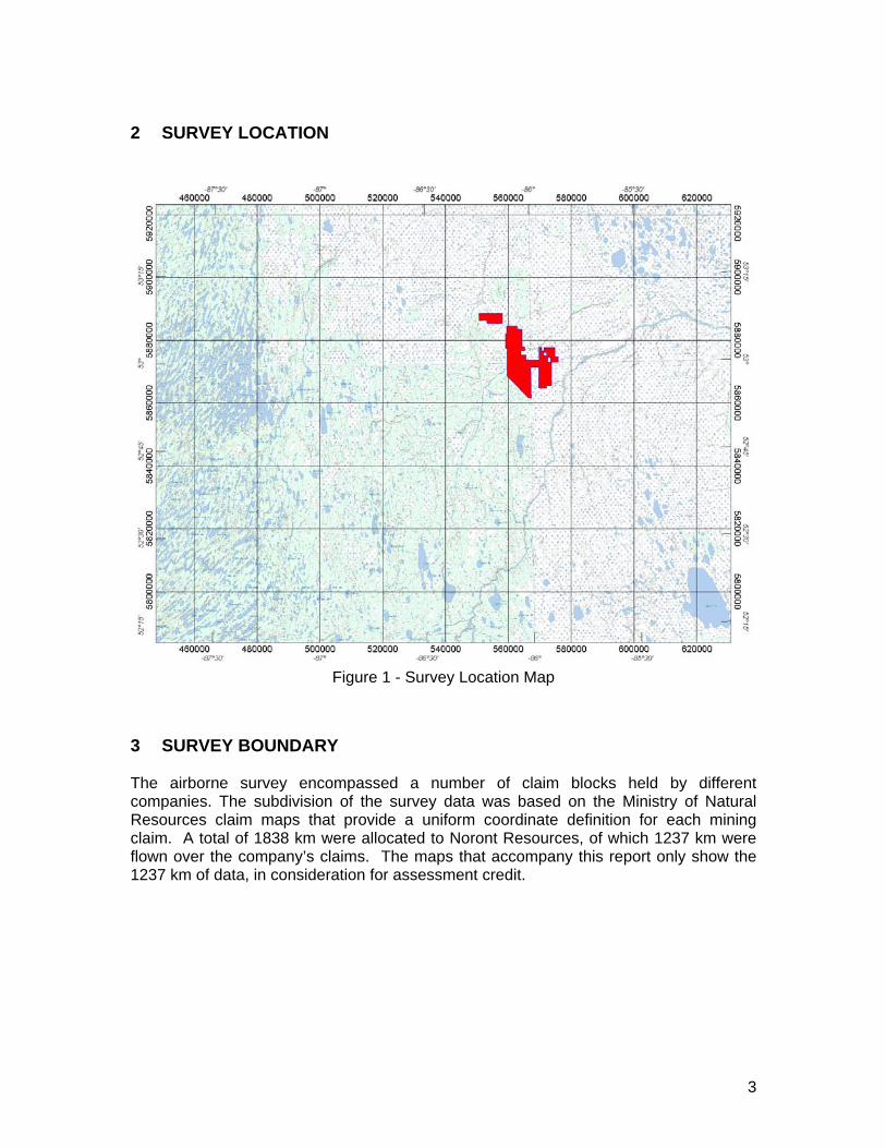
2 SURVEY LOCATION

Figure 1 - Survey Location Map

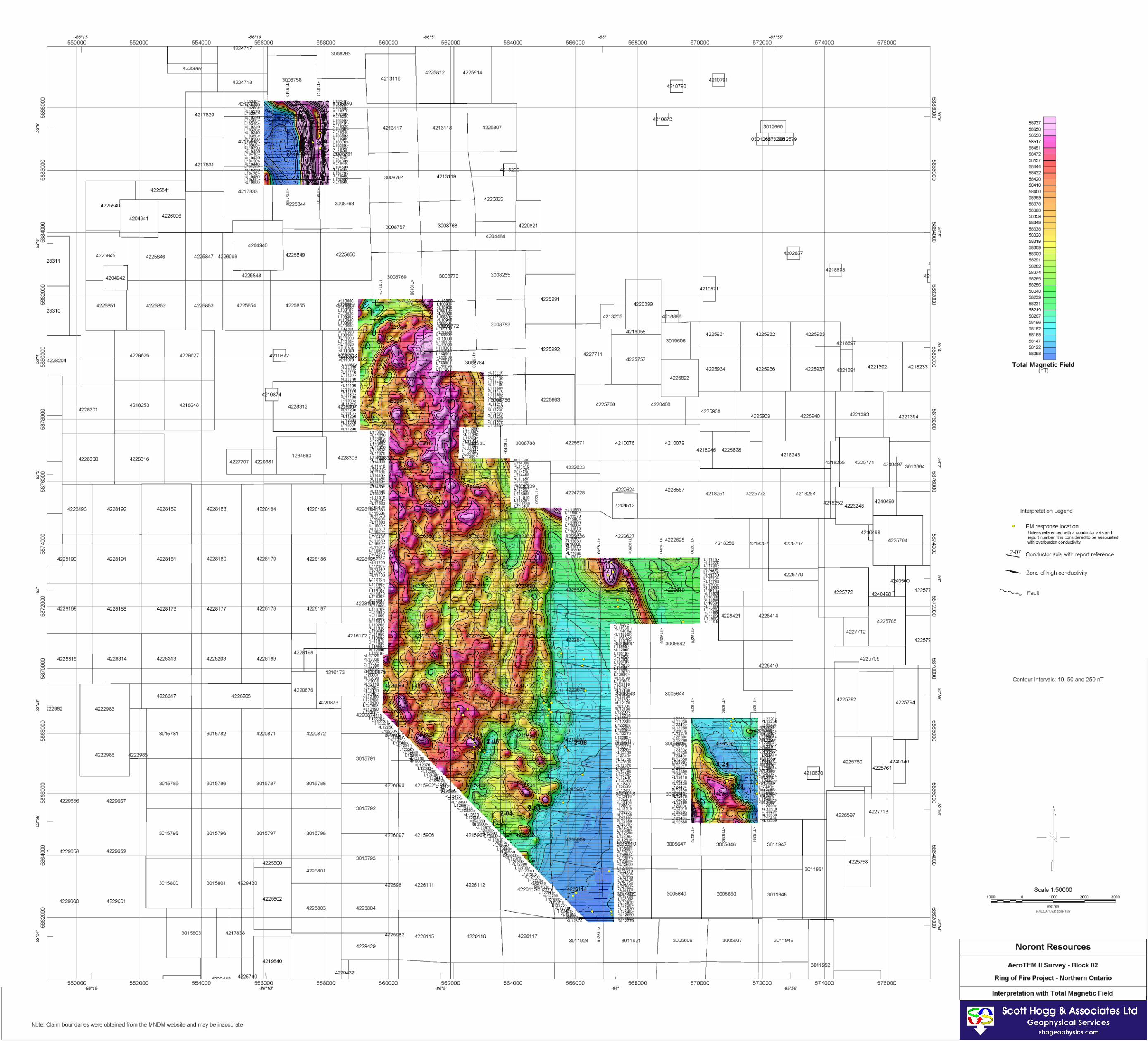
3 SURVEY BOUNDARY The airborne survey encompassed a number of claim blocks held by different companies. The subdivision of the survey data was based on the Ministry of Natural Resources claim maps that provide a uniform coordinate definition for each mining claim. A total of 1838 km were allocated to Noront Resources, of which 1237 km were flown over the company’s claims. The maps that accompany this report only show the 1237 km of data, in consideration for assessment credit.

4

4 AIRBORNE SURVEY

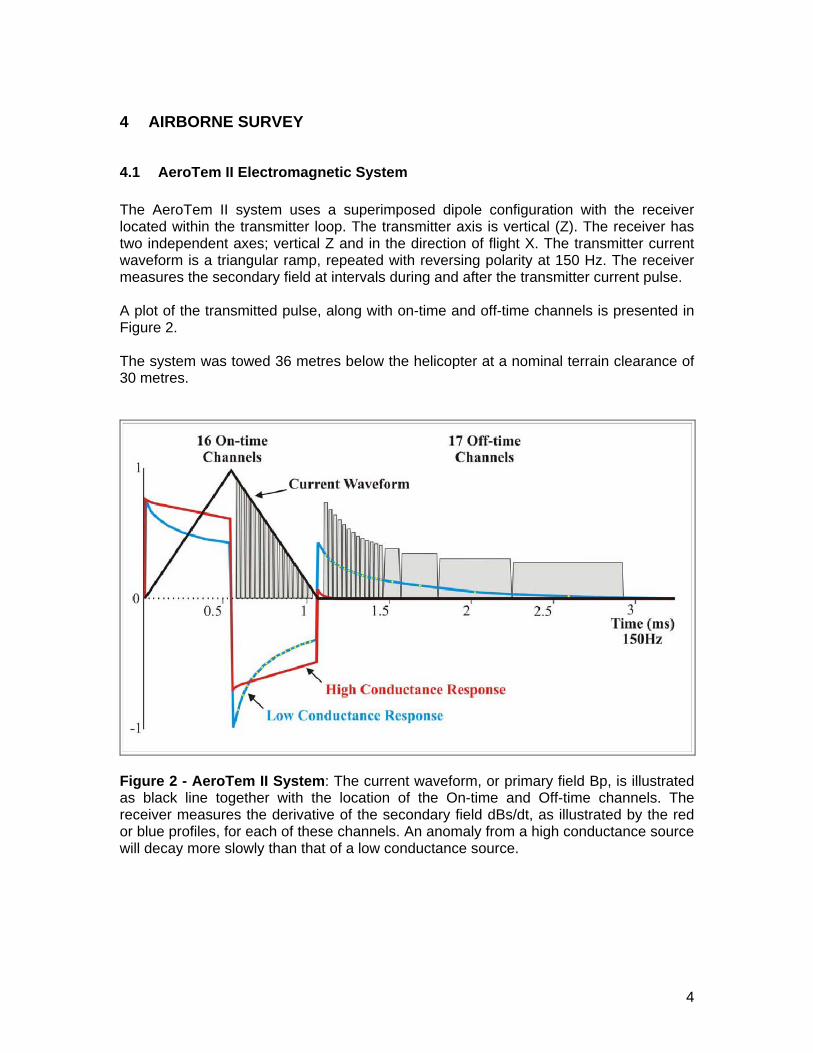
4.1 AeroTem II Electromagnetic System The AeroTem II system uses a superimposed dipole configuration with the receiver located within the transmitter loop. The transmitter axis is vertical (Z). The receiver has two independent axes; vertical Z and in the direction of flight X. The transmitter current waveform is a triangular ramp, repeated with reversing polarity at 150 Hz. The receiver measures the secondary field at intervals during and after the transmitter current pulse. A plot of the transmitted pulse, along with on-time and off-time channels is presented in Figure 2. The system was towed 36 metres below the helicopter at a nominal terrain clearance of 30 metres.

Figure 2 - AeroTem II System: The current waveform, or primary field Bp, is illustrated as black line together with the location of the On-time and Off-time channels. The receiver measures the derivative of the secondary field dBs/dt, as illustrated by the red or blue profiles, for each of these channels. An anomaly from a high conductance source will decay more slowly than that of a low conductance source.

5

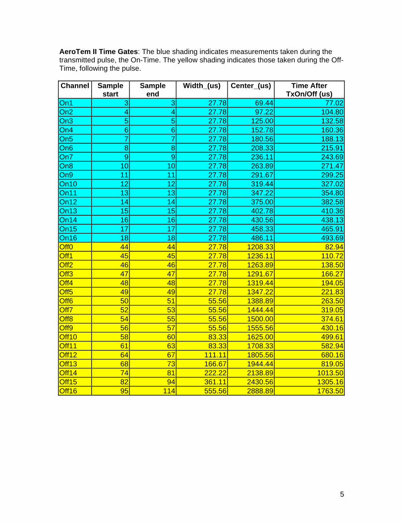
AeroTem II Time Gates: The blue shading indicates measurements taken during the transmitted pulse, the On-Time. The yellow shading indicates those taken during the Off-Time, following the pulse. Channel Sample

start Sample

end Width_(us) Center_(us) Time After

TxOn/Off (us) On1 3 3 27.78 69.44 77.02On2 4 4 27.78 97.22 104.80On3 5 5 27.78 125.00 132.58On4 6 6 27.78 152.78 160.36On5 7 7 27.78 180.56 188.13On6 8 8 27.78 208.33 215.91On7 9 9 27.78 236.11 243.69On8 10 10 27.78 263.89 271.47On9 11 11 27.78 291.67 299.25On10 12 12 27.78 319.44 327.02On11 13 13 27.78 347.22 354.80On12 14 14 27.78 375.00 382.58On13 15 15 27.78 402.78 410.36On14 16 16 27.78 430.56 438.13On15 17 17 27.78 458.33 465.91On16 18 18 27.78 486.11 493.69Off0 44 44 27.78 1208.33 82.94Off1 45 45 27.78 1236.11 110.72Off2 46 46 27.78 1263.89 138.50Off3 47 47 27.78 1291.67 166.27Off4 48 48 27.78 1319.44 194.05Off5 49 49 27.78 1347.22 221.83Off6 50 51 55.56 1388.89 263.50Off7 52 53 55.56 1444.44 319.05Off8 54 55 55.56 1500.00 374.61Off9 56 57 55.56 1555.56 430.16Off10 58 60 83.33 1625.00 499.61Off11 61 63 83.33 1708.33 582.94Off12 64 67 111.11 1805.56 680.16Off13 68 73 166.67 1944.44 819.05Off14 74 81 222.22 2138.89 1013.50Off15 82 94 361.11 2430.56 1305.16Off16 95 114 555.56 2888.89 1763.50

6

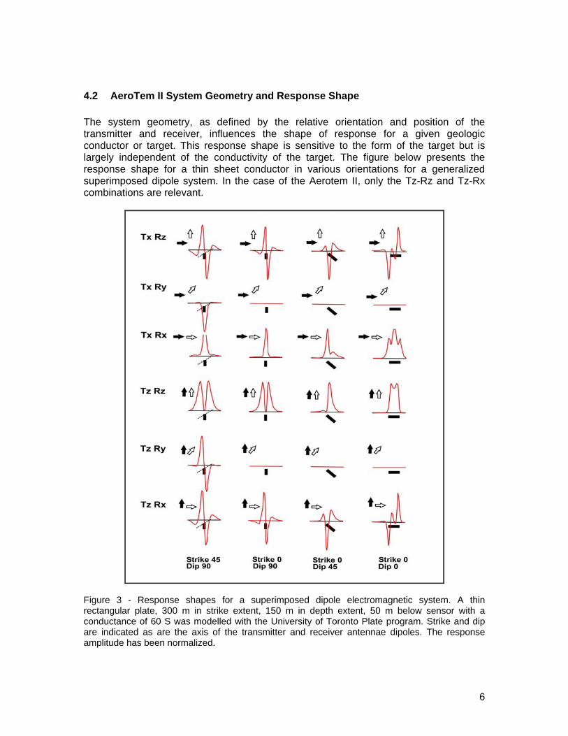
4.2 AeroTem II System Geometry and Response Shape The system geometry, as defined by the relative orientation and position of the transmitter and receiver, influences the shape of response for a given geologic conductor or target. This response shape is sensitive to the form of the target but is largely independent of the conductivity of the target. The figure below presents the response shape for a thin sheet conductor in various orientations for a generalized superimposed dipole system. In the case of the Aerotem II, only the Tz-Rz and Tz-Rx combinations are relevant.

Figure 3 - Response shapes for a superimposed dipole electromagnetic system. A thin rectangular plate, 300 m in strike extent, 150 m in depth extent, 50 m below sensor with a conductance of 60 S was modelled with the University of Toronto Plate program. Strike and dip are indicated as are the axis of the transmitter and receiver antennae dipoles. The response amplitude has been normalized.

7

The Tz-Rz configuration is minimum coupled with a vertical thin sheet when the system is directly overhead. This results in an "M" shaped response. As the horizontal thickness of the conductor increases, induced currents can flow across the sheet and the central null is reduced. When the width is of the same order as the other dimensions, like a sphere, the null disappears completely and a simple broad peak over the conductor results. As the dip of the sheet decreases an asymmetry of the side lobes becomes evident with the greater amplitude on the down dip side. This asymmetry is most notable between about 60 and 30 degrees. With shallower dip the smaller lobe is relatively very weak and a slightly asymmetric single peak is the dominant signature. In the case of near horizontal conducting layers the response amplitude stabilizes within the unit but if the edges are sharply defined, edge effects will be noted.

4.3 Magnetometers Two Geometrics optically pumped cesium sensors recorded the total magnetic field. One was located on the electromagnetic bird, 38 metres below the helicopter at a nominal terrain clearance of 31 metres, the second sensor was towed 21 metres below the helicopter at a nominal terrain clearance of 44 metres. A magnetic base station was located at the base of operations and recorded variations were used for diurnal correction

8

5 COMPILATION AND PRESENTATION

5.1 Total Field Magnetics The magnetic data from a lower sensor in the EM bird was not available throughout the survey. For consistency, the magnetic data recorded at the nominal terrain clearance of 44 metres has been used for presentation and analysis. Variations recorded by the magnetic base station were subtracted to remove diurnal magnetic variation. The corrected profile, provided by Aeroquest, was gridded using at 25 metre cell size. In addition to the Total Magnetic Field, the following two map enhancements were calculated for interpretive use.

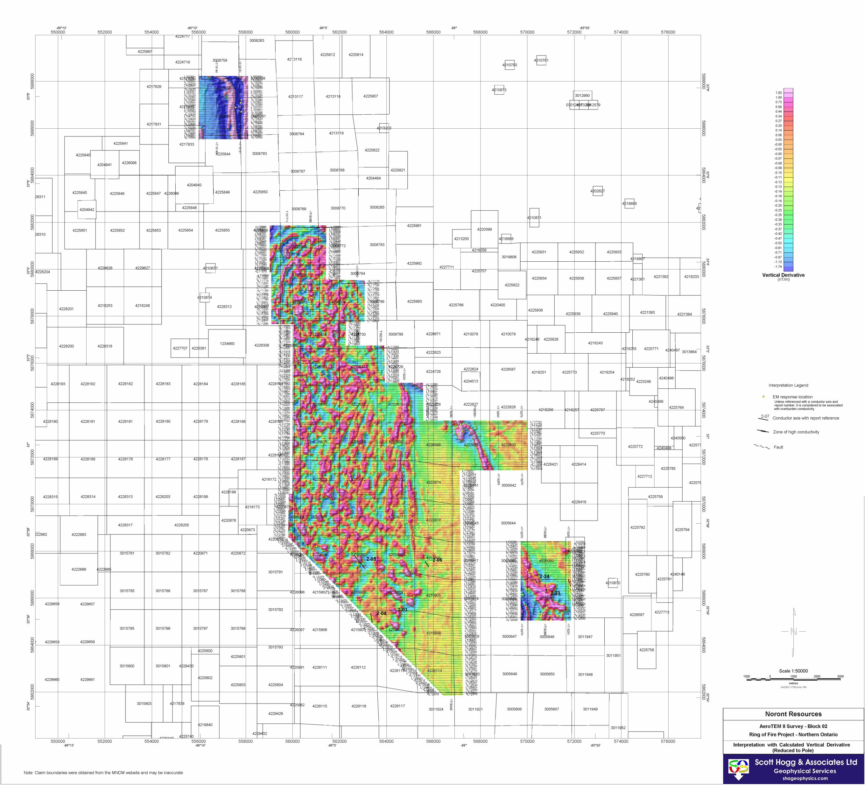
5.2 Pole Reduced Vertical Magnetic Gradient This map has combined two map enhancements. The pole reduction process alters the shape of the magnetic anomalies to appear as they would if the inclination of the magnetic field were vertical. The inclination of the magnetic field in the survey area is about 78 degrees and the difference is subtle but notable. The vertical magnetic gradient sharpens and enhances the response from shallow magnetic sources relative to those originating at greater depth. The combined pole reduction and vertical gradient process will provide a positive peak directly over a vertical dipping, inductively magnetized source. A negative side-lobe will surround the anomaly. If the horizontal dimensions of the magnetic unit are significantly larger than the height above source, the zero gradient contour will tend to follow the magnetic contact.

5.3 Apparent Magnetic Susceptibility The amplitude of a magnetic anomaly is a function of the size, depth, form and magnetic susceptibility of the source. The apparent susceptibility process approximates the underlying geology by a regular array of vertical prism forms at uniform depth. Each rectangular prism is 25 metres in horizontal dimension, with large depth extent and an upper surface 25 metres below ground. The process assigns a susceptibility to each prism such that the combined result would emulate the observed total field map. The resulting map approximates the magnetic susceptibility of the underlying geology. The susceptibility values presented are not absolute but are relative to a mean map value of zero. The change from one level to another represents the susceptibility contrast. The Palaeozoic limestone and glacial cover will have essentially no magnetic contribution. In the bedrock the lowest susceptibility is expected with the metasedimentary rocks with increasing susceptibility through the acid to intermediate to mafic volcanic rock sequence.

9

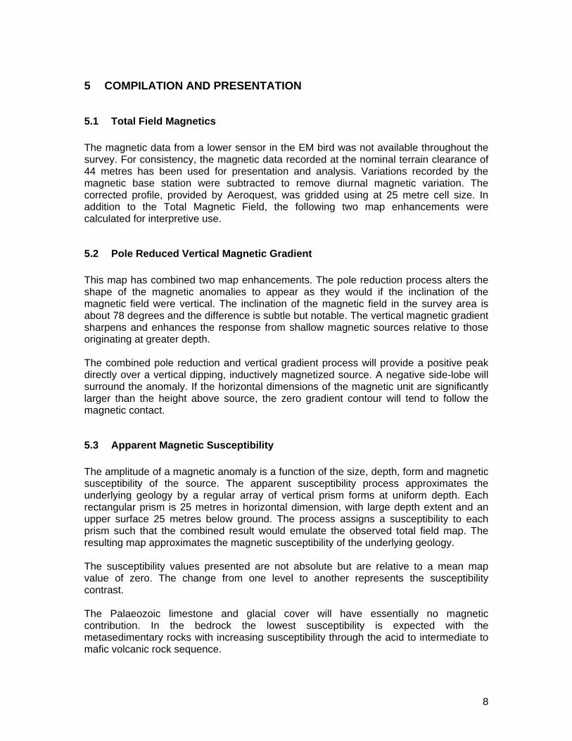
5.4 Electromagnetic Time Constant Tau The primary electromagnetic field is created by the current flowing in the transmitter loop. It induces current flow in the underlying ground, which in turn, creates a secondary electromagnetic field. This secondary magnetic field B induces a voltage in the receiver which is proportional to dB/dt, the rate of change of the secondary field passing through the coil. An estimate of the B field can be derived by either digital or electronic integration of the directly measured signal dB/dt. The basic time-domain electromagnetic anomaly can be expressed as an exponential.

B = ke-t/τ where B is the amplitude of the B-field signal, k is a constant related to the size, shape and depth of the source, t is time in microseconds and τ is the time-constant Tau. A large conductive body will have a large Tau and thus the signal will decay slowly. A small poor conductor will have a small Tau and thus decay quickly.

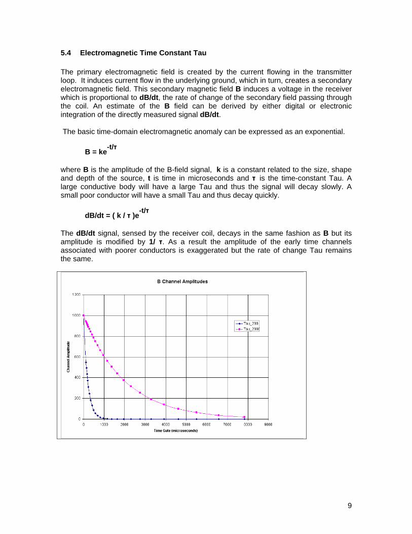
dB/dt = ( k / τ )e-t/τ The dB/dt signal, sensed by the receiver coil, decays in the same fashion as B but its amplitude is modified by 1/ τ. As a result the amplitude of the early time channels associated with poorer conductors is exaggerated but the rate of change Tau remains the same.

10

A value for the apparent time constant Tau can be calculated using any two channels. Tau = -(t1-t2) / log( Ampliude1/Amplitude2 ) The actual signal measured is a sum of exponentials. A time constant calculated using early channels will predominantly reflect the shorter time constants and one based on late channels will predominantly reflect the longer time constants. The Zoff array channel contains the signal amplitude for each of the system time gates. The time constant Tau was calculated for each successive pair of gates and the results, in units of microseconds, were stored in the SHA_Tau array channel. The last channel element of SHA_Tau array contains the largest time constant of the sequence. As the channel amplitudes decrease, noise will enter the calculation, with increased sensitivity to the denominator, Amplitude2. The calculation of the time constant was suspended when signal levels were less than about 10 nT/s.

5.5 Electromagnetic Conductance Calculation A variety of related measurement units are often used to quantify an electromagnetic anomaly. Electrical resistance is measured in ohms, resistivity in ohm-m. Conductance is the inverse of resistance and measured in mhos or Siemens. Conductivity is the inverse of resistivity is measured in mhos/m or Siemens/m. Conductance reflects not only the conductivity but also the size of the anomaly source. For a time-domain system conductance can be derived from the time-constant Tau and is largely independent of depth. A channel SHA_conductance has been created on the

11

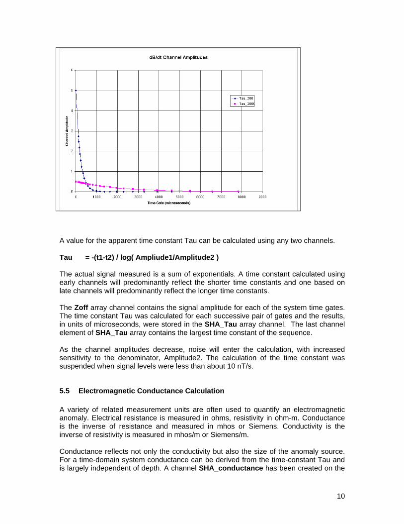
assumption that the conductor is a flat-lying plate, 100m. by 100m. This is the same reference model used by Aeroquest. The point by point calculation has been filtered along line to stabilize the calculation and the result, in Siemens, has been presented in both profile and gridded form. As a very general rule, conductance indications above 10 Siemens are anticipated for VMS deposits and can exceed 100 Siemens for MMS nickel deposits.

This AeroTem response diagram is copied from the Aeroquest report. The system is insensitive to a conductance less than 0.5 S and is optimal in the off-time to the range of 5 to 50 S. The on-time response is optimal for conductance values of 50 S and greater.

12

6 INTERPRETATION OVERVIEW The McFaulds VMS deposits discovered by Spider-KWG are copper-zinc bearing and have been compared to those in the Matagami area of Quebec. An electromagnetic signature has been identified at the sites, initially by the fixed-wing GeoTem system, as well as the VTEM and AeroTem helicopter systems. In addition to a conductivity anomaly the deposits tend to have an associated magnetic signature. The conductivity expectations for a zinc rich VMS deposit are tempered by the fact that zinc sulphide is not a notable conductor as illustrated in table 1, below. Due to the usually associated presence of chalcopyrite and pyrrhotite, copper-zinc VMS deposits are often moderately conductive. It might be speculated that very rich zinc deposits may exist but remain undetected since the primary exploration method, electromagnetics, would be ineffective for a pure sphalerite deposit. The Noront Eagle One is a copper nickel MMS deposit. It also provided an electromagnetic signature on the fixed-wing and helicopter electromagnetic systems and has an associated magnetic anomaly. Nickel deposits can have very high associated conductivity. A third deposit type in the area is the Spider, KWG, Freewest chrome-platinum- palladium discovery in a peridotite host. Conductivity expectations for such mineralization are variable; chromite is not a notable conductor but other sulphides in the formation may create a significant electromagnetic anomaly. The peridotite host is a notable magnetic rock. Mineral Conductivity (mhos/m) Resistivity (ohm-m)

Millerite NiS 3333333.33 3.00E-07 Niccolite NiAs 50000.00 2.00E-05 Pyrrhotite FeS 10000.00 1.00E-04 Arsenopyrite FeAsS 1000.00 1.00E-03 Galena PbS 500.00 2.00E-03 Chalcopyrite CuFeS2 250.00 4.00E-03 Graphite C 100.00 1.00E-02 Cassiterite SnO2 5.00 2.00E-01 Pyrite FeS2 3.33 3.00E-01 Magnetite Fe3O4 3.33 3.00E-01 Hematite Fe2O3 0.10 1.00E+01 Sphalerite ZnS 0.01 1.00E+02 In the McFaulds Lake environment, a higher conductivity may be encouraging but is not considered a prerequisite for a significant deposit. Higher conductances might be considered more typical of the copper and nickel bearing mineralization while low to moderate conductances might be considered more typical of the copper-zinc or the chromitite-platinum group mineralization.

13

The conductivity anomalies of the known VMS deposits in the area are of limited size. This attribute of limited strike length is typical for VMS deposits in general. An isolated response, limited to a few flight lines is a normal expectation. A coincident or adjacent magnetic signature is also a common VMS attribute. A similar scale magnetic anomaly might be considered an encouraging factor but it should not be considered a prerequisite. 7 INTERPRETATION PROCEDURE A preliminary anomaly identification process was carried out by SHA using data provided by the Aeroquest field crew. The uncorrected electromagnetic profile data was reviewed, line by line, and anomalies of potential interest were identified. The location of the anomalies on each line was evaluated in a map presentation and conductor axes were interpreted. During this initial review of the profile data a database channel named Anom was created which was flagged with a numeric value when a response of possible interest was noted. The purpose of this channel was to provide a convenient profile-to-map interface for revisiting and correlating profile and map events. These Anom events were plotted as symbols on the preliminary interpretation maps. They are not anomalies in the traditional sense but simply working reference points used in the interpretation process. These references have been carried forward into the final database. Those not associated with interpreted conductor axes of interest are attributed to conductive overburden. The geophysical data was then corrected and processed internally by the contractor Aeroquest. As part of this operation, Aeroquest has independently provided a "standard" report and maps with conductive responses symbolized. The associated report, maps and digital data has been divided along property boundaries and provided to each participant in the overall program. The Aeroquest anomalies and other interpretive information are not referred to and do not have any bearing on the content of this interpretation and report. However, the corrected profile database, provided by Aeroquest, has been used for the interpretation and processing by Scott Hogg & Associates Ltd. Digital database channels, created by Aeroquest, have been preserved. The analysis of the geophysical data was carried out on the full survey block without regard for property boundaries within. The corrected electromagnetic profile data was reviewed, line by line, and anomalies of potential exploration interest were identified. Responses that were believed to simply reflect conductive overburden are not included or discussed further. The location of the anomalies on each line was evaluated in a map presentation and conductor axes were interpreted. The conductors have been provided a report identifier “ Area# - reference# “. No significance is attached to the numerical sequence. The interpretation map was then divided in accordance with property boundaries and the map contents and related geophysical comments for the specific client are included with this report.

14

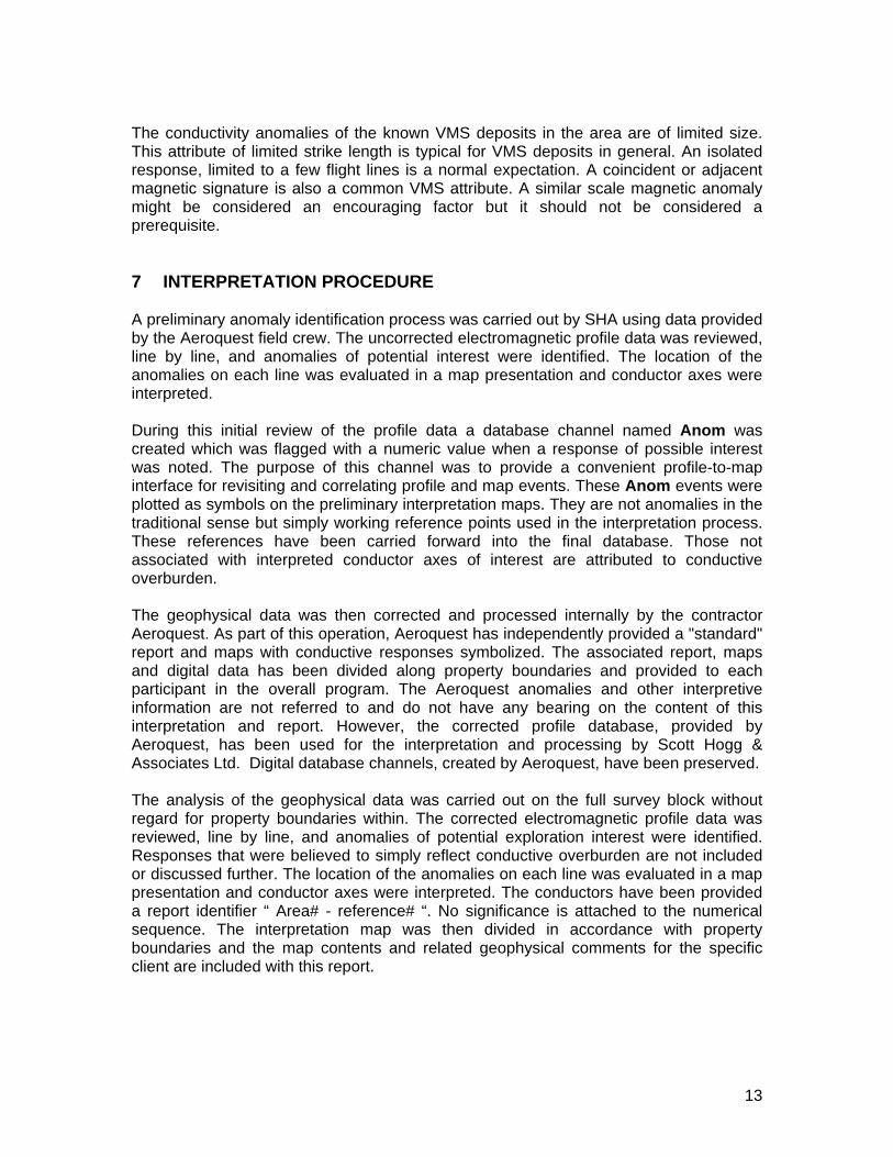
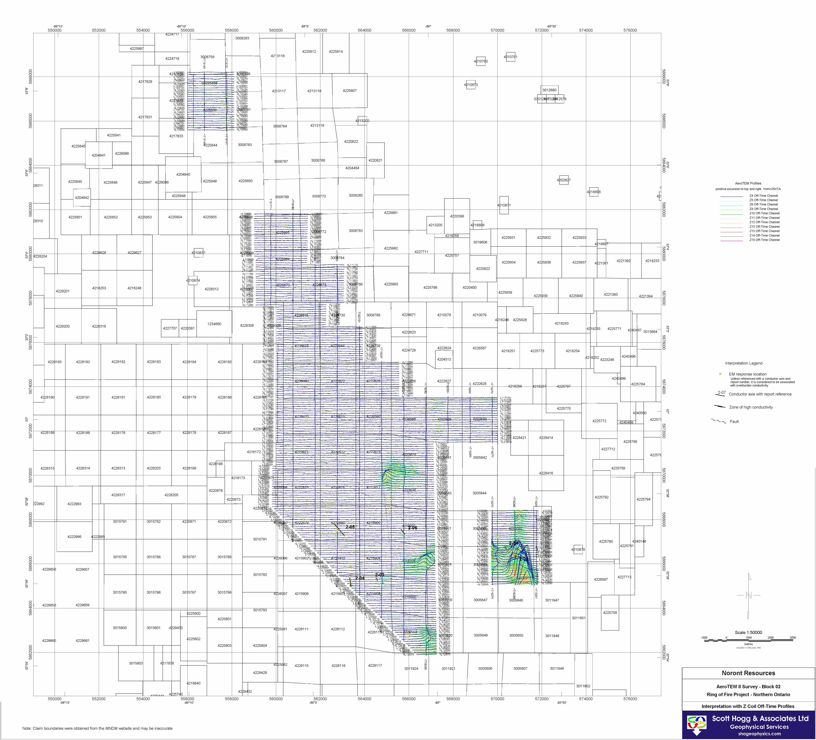
8 DISCUSSION AND RECOMMENDATIONS The following discussion, of the interpreted electromagnetic anomalies, is organized by conductor reference number. A difficulty with the map presentation of electromagnetic data is the large dynamic range of the response and the variety of information available; on-time, off-time, Z-axis and X-axis receiver configurations, all with multiple time-gates. This information is viewable on a line by line basis but not in useful map presentations. For most of the anomalies a profile response figure, from a representative flight line, has been included to illustrate the anomaly detail. The Z-on response is presented with an expanded vertical scale, suited to identifying the weaker anomalies. The typical noise threshold of the system, about 5 nT/s, is discernible at the scale chosen. The corresponding magnetic and conductance profile is also presented. The horizontal scale units are UTM easting coordinates which can be identified on the map for chosen flight line. Follow-up investigation is recommended where a clear indication of a bedrock conductor has been interpreted. The highest priority recommendation was reserved for those with a high conductance that can often indicate major sulphide mineralization. Lower priorities are suggested for lower conductance indications; however, it is important to again note that the lower conductance values can be associated economic mineralization such as thinner zones of high value minerals or large zones of a less conductive mineral such as zinc.

15

Anomaly 2-3

2-03 A weak one line response on the edge of magnetic zone that extends to the

northwest. The profile shape suggests a thin steeply dipping source but in light of the low calculated conductance of about 1 S, no further investigation is recommended on the basis of the geophysical data.

16

Anomaly 2-04

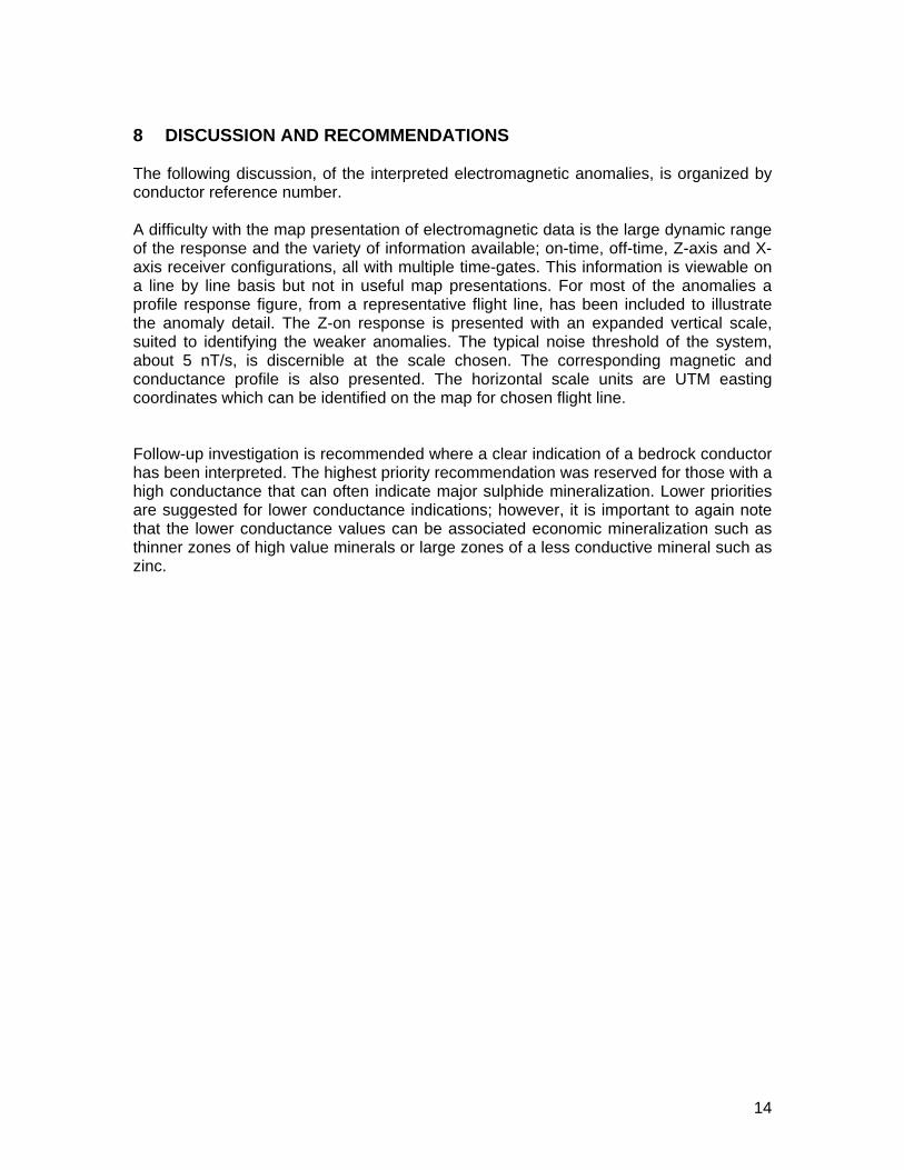
2-04 This broad low amplitude anomaly has little late time response and thus a

negligible calculated conductance. A weak parallel magnetic axis is adjacent to the east and is considered an indication that the source may be of basement origin; however, no further investigation is recommended.

17

Anomaly 2-05

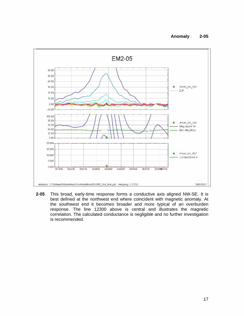
2-05 This broad, early-time response forms a conductive axis aligned NW-SE. It is

best defined at the northwest end where coincident with magnetic anomaly. At the southwest end it becomes broader and more typical of an overburden response. The line 12300 above is central and illustrates the magnetic correlation. The calculated conductance is negligible and no further investigation is recommended.

18

Anomaly 2-06

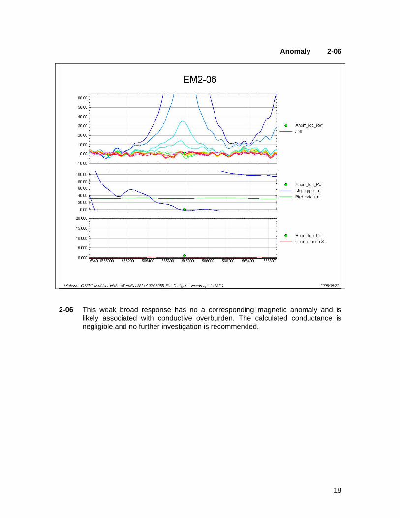
2-06 This weak broad response has no a corresponding magnetic anomaly and is

likely associated with conductive overburden. The calculated conductance is negligible and no further investigation is recommended.

19

Anomaly 2-23

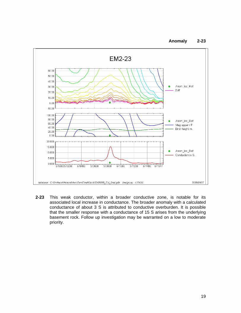
2-23 This weak conductor, within a broader conductive zone, is notable for its

associated local increase in conductance. The broader anomaly with a calculated conductance of about 3 S is attributed to conductive overburden. It is possible that the smaller response with a conductance of 15 S arises from the underlying basement rock. Follow up investigation may be warranted on a low to moderate priority.

20

Anomaly 2-24

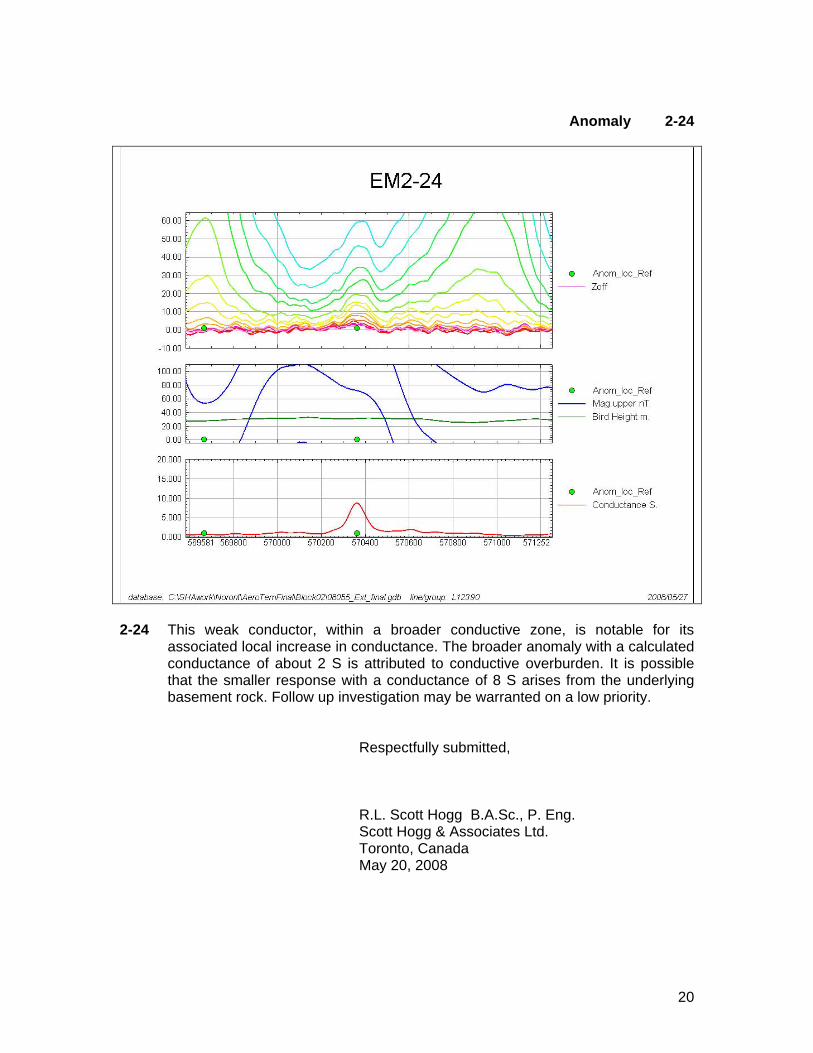
2-24 This weak conductor, within a broader conductive zone, is notable for its

associated local increase in conductance. The broader anomaly with a calculated conductance of about 2 S is attributed to conductive overburden. It is possible that the smaller response with a conductance of 8 S arises from the underlying basement rock. Follow up investigation may be warranted on a low priority.

Respectfully submitted, R.L. Scott Hogg B.A.Sc., P. Eng. Scott Hogg & Associates Ltd. Toronto, Canada May 20, 2008

21

APPENDIX – CONTRACTOR REPORT DETAILS

Report on a Helicopter-Borne AeroTEM System Electromagnetic

& Magnetic Survey

Aeroquest Job # 08055

Extension Project McFaulds Lake Camp, Ontario, Canada NTS 043C13, 043D16, 043E01, 043F04

For

Billiken Management Services Inc.

by

7687 Bath Road, Mississauga, ON, L4T 3T1

Tel: (905) 672-9129 Fax: (905) 672-7083 www.aeroquest.ca

Report date: February 2008

Report on a Helicopter-Borne AeroTEM System Electromagnetic & Magnetic Survey

Aeroquest Job # 08055

Extension Project McFaulds Lake Camp, Ontario, Canada NTS 043C13, 043D16, 043E01, 043F04

For

Billiken Management Services Inc. Suite 1000, 15 Toronto Street,

Toronto, Ontario. M5C 2E3

by

7687 Bath Road, Mississauga, ON, L4T 3T1

Tel: (905) 672-9129 Fax: (905) 672-7083 www.aeroquest.ca

Report date: February 2008

Job # 08055

Aeroquest International - Report on a Helicopter-Borne AeroTEM System Electromagnetic & Magnetic Survey

3

3. SURVEY SPECIFICATIONS AND PROCEDURES The survey specifications are summarised in the following table:

Project Name

Line Spacing (metres)

Line Direction

Survey Coverage(line-km)

Date flown

Extension 100 E-W (90º) 5279.7 Nov 27th to Dec 16th , 2007

Table 1. Survey specifications summary

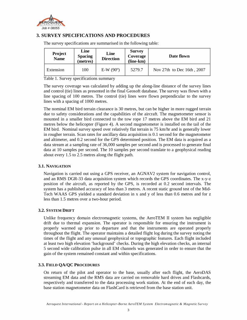
The survey coverage was calculated by adding up the along-line distance of the survey lines and control (tie) lines as presented in the final Geosoft database. The survey was flown with a line spacing of 100 metres. The control (tie) lines were flown perpendicular to the survey lines with a spacing of 1000 metres.

The nominal EM bird terrain clearance is 30 metres, but can be higher in more rugged terrain due to safety considerations and the capabilities of the aircraft. The magnetometer sensor is mounted in a smaller bird connected to the tow rope 17 metres above the EM bird and 21 metres below the helicopter (Figure 4). A second magnetometer is installed on the tail of the EM bird. Nominal survey speed over relatively flat terrain is 75 km/hr and is generally lower in rougher terrain. Scan rates for ancillary data acquisition is 0.1 second for the magnetometer and altimeter, and 0.2 second for the GPS determined position. The EM data is acquired as a data stream at a sampling rate of 36,000 samples per second and is processed to generate final data at 10 samples per second. The 10 samples per second translate to a geophysical reading about every 1.5 to 2.5 metres along the flight path.

3.1. NAVIGATION

Navigation is carried out using a GPS receiver, an AGNAV2 system for navigation control, and an RMS DGR-33 data acquisition system which records the GPS coordinates. The x-y-z position of the aircraft, as reported by the GPS, is recorded at 0.2 second intervals. The system has a published accuracy of less than 3 metres. A recent static ground test of the Mid-Tech WAAS GPS yielded a standard deviation in x and y of less than 0.6 metres and for z less than 1.5 metres over a two-hour period.

3.2. SYSTEM DRIFT

Unlike frequency domain electromagnetic systems, the AeroTEM II system has negligible drift due to thermal expansion. The operator is responsible for ensuring the instrument is properly warmed up prior to departure and that the instruments are operated properly throughout the flight. The operator maintains a detailed flight log during the survey noting the times of the flight and any unusual geophysical or topographic features. Each flight included at least two high elevation ‘background’ checks. During the high elevation checks, an internal 5 second wide calibration pulse in all EM channels was generated in order to ensure that the gain of the system remained constant and within specifications.

3.3. FIELD QA/QC PROCEDURES

On return of the pilot and operator to the base, usually after each flight, the AeroDAS streaming EM data and the RMS data are carried on removable hard drives and Flashcards, respectively and transferred to the data processing work station. At the end of each day, the base station magnetometer data on FlashCard is retrieved from the base station unit.

Job # 08055


4

Data verification and quality control includes a comparison of the acquired GPS data with the flight plan; verification and conversion of the RMS data to an ASCII format XYZ data file; verification of the base station magnetometer data and conversion to ASCII format XYZ data; and loading, processing and conversion of the steaming EM data from the removable hard drive. All data is then merged to an ASCII XYZ format file which is then imported to an Oasis database for further QA/QC and for the production of preliminary EM, magnetic contour, and flight path maps.

Survey lines which show excessive deviation from the intended flight path are re-flown. Any line or portion of a line on which the data quality did not meet the contract specification was noted and reflown.

4. AIRCRAFT AND EQUIPMENT

4.1. AIRCRAFT

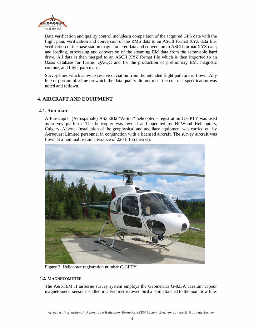
A Eurocopter (Aerospatiale) AS350B2 "A-Star" helicopter - registration C-GPTY was used as survey platform. The helicopter was owned and operated by Hi-Wood Helicopters, Calgary, Alberta. Installation of the geophysical and ancillary equipment was carried out by Aeroquest Limited personnel in conjunction with a licensed aircraft. The survey aircraft was flown at a nominal terrain clearance of 220 ft (65 metres).

Figure 3. Helicopter registration number C-GPTY

4.2. MAGNETOMETER

The AeroTEM II airborne survey system employs the Geometrics G-823A caesium vapour magnetometer sensor installed in a two metre towed bird airfoil attached to the main tow line,

Job # 08055


5

21 metres below the helicopter (Figure 4). The sensitivity of the magnetometer is 0.001 nanoTesla at a 0.1 second sampling rate. The nominal ground clearance of the magnetometer bird is 51 metres (170 ft.). The magnetic data is recorded at 10 Hz by the RMS DGR-33.

4.3. MAGNETOMETER II

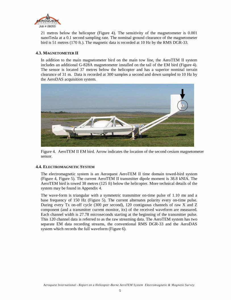
In addition to the main magnetometer bird on the main tow line, the AeroTEM II system includes an additional G-828A magnetometer installed on the tail of the EM bird (Figure 4). The sensor is located 37 metres below the helicopter and has a superior nominal terrain clearance of 31 m. Data is recorded at 300 samples a second and down sampled to 10 Hz by the AeroDAS acquisition system.

Figure 4. AeroTEM II EM bird. Arrow indicates the location of the second cesium magnetometer sensor.

4.4. ELECTROMAGNETIC SYSTEM

The electromagnetic system is an Aeroquest AeroTEM II time domain towed-bird system (Figure 4, Figure 5). The current AeroTEM II transmitter dipole moment is 38.8 kNIA. The AeroTEM bird is towed 38 metres (125 ft) below the helicopter. More technical details of the system may be found in Appendix 4.

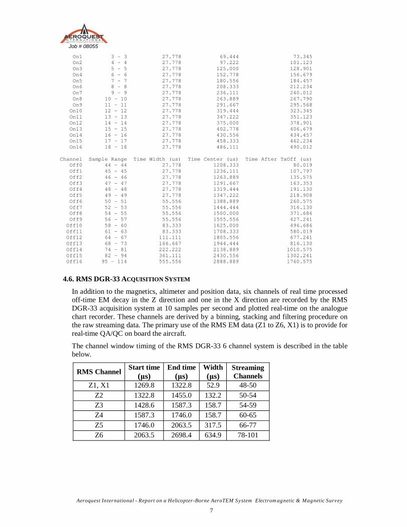
The wave-form is triangular with a symmetric transmitter on-time pulse of 1.10 ms and a base frequency of 150 Hz (Figure 5). The current alternates polarity every on-time pulse. During every Tx on-off cycle (300 per second), 120 contiguous channels of raw X and Z component (and a transmitter current monitor, itx) of the received waveform are measured. Each channel width is 27.78 microseconds starting at the beginning of the transmitter pulse. This 120 channel data is referred to as the raw streaming data. The AeroTEM system has two separate EM data recording streams, the conventional RMS DGR-33 and the AeroDAS system which records the full waveform (Figure 6).

Job # 08055


6

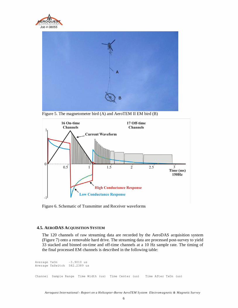
Figure 5. The magnetometer bird (A) and AeroTEM II EM bird (B)

Figure 6. Schematic of Transmitter and Receiver waveforms

4.5. AERODAS ACQUISITION SYSTEM

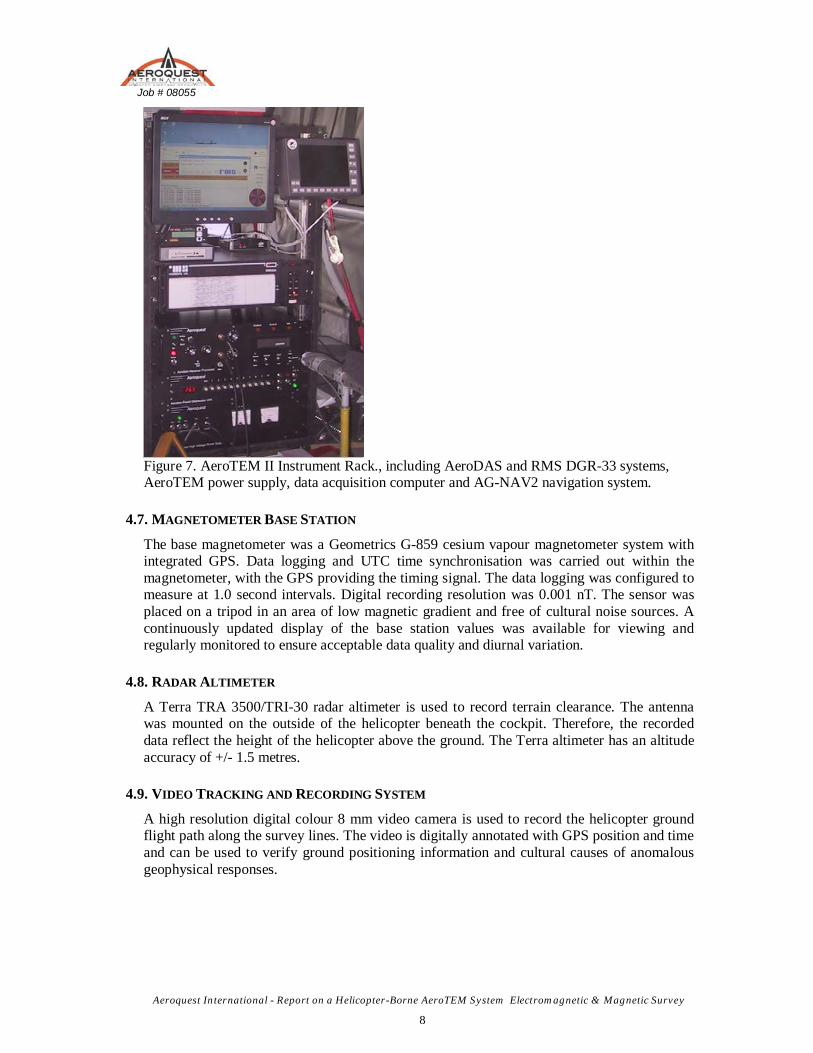
The 120 channels of raw streaming data are recorded by the AeroDAS acquisition system (Figure 7) onto a removable hard drive. The streaming data are processed post-survey to yield 33 stacked and binned on-time and off-time channels at a 10 Hz sample rate. The timing of the final processed EM channels is described in the following table:

Average TxOn -3.9010 us Average TxSwitch 582.2389 us Channel Sample Range Time Width (us) Time Center (us) Time After TxOn (us)

Job # 08055


7

On1 3 - 3 27.778 69.444 73.345 On2 4 - 4 27.778 97.222 101.123 On3 5 - 5 27.778 125.000 128.901 On4 6 - 6 27.778 152.778 156.679 On5 7 - 7 27.778 180.556 184.457 On6 8 - 8 27.778 208.333 212.234 On7 9 - 9 27.778 236.111 240.012 On8 10 - 10 27.778 263.889 267.790 On9 11 - 11 27.778 291.667 295.568 On10 12 - 12 27.778 319.444 323.345 On11 13 - 13 27.778 347.222 351.123 On12 14 - 14 27.778 375.000 378.901 On13 15 - 15 27.778 402.778 406.679 On14 16 - 16 27.778 430.556 434.457 On15 17 - 17 27.778 458.333 462.234 On16 18 - 18 27.778 486.111 490.012 Channel Sample Range Time Width (us) Time Center (us) Time After TxOff (us) Off0 44 - 44 27.778 1208.333 80.019 Off1 45 - 45 27.778 1236.111 107.797 Off2 46 - 46 27.778 1263.889 135.575 Off3 47 - 47 27.778 1291.667 163.353 Off4 48 - 48 27.778 1319.444 191.130 Off5 49 - 49 27.778 1347.222 218.908 Off6 50 - 51 55.556 1388.889 260.575 Off7 52 - 53 55.556 1444.444 316.130 Off8 54 - 55 55.556 1500.000 371.686 Off9 56 - 57 55.556 1555.556 427.241 Off10 58 - 60 83.333 1625.000 496.686 Off11 61 - 63 83.333 1708.333 580.019 Off12 64 - 67 111.111 1805.556 677.241 Off13 68 - 73 166.667 1944.444 816.130 Off14 74 - 81 222.222 2138.889 1010.575 Off15 82 - 94 361.111 2430.556 1302.241 Off16 95 - 114 555.556 2888.889 1760.575

4.6. RMS DGR-33 ACQUISITION SYSTEM

In addition to the magnetics, altimeter and position data, six channels of real time processed off-time EM decay in the Z direction and one in the X direction are recorded by the RMS DGR-33 acquisition system at 10 samples per second and plotted real-time on the analogue chart recorder. These channels are derived by a binning, stacking and filtering procedure on the raw streaming data. The primary use of the RMS EM data (Z1 to Z6, X1) is to provide for real-time QA/QC on board the aircraft.

The channel window timing of the RMS DGR-33 6 channel system is described in the table below.

RMS Channel Start time (μs)

End time(μs)

Width(μs)

Streaming Channels

Z1, X1 1269.8 1322.8 52.9 48-50 Z2 1322.8 1455.0 132.2 50-54 Z3 1428.6 1587.3 158.7 54-59 Z4 1587.3 1746.0 158.7 60-65 Z5 1746.0 2063.5 317.5 66-77 Z6 2063.5 2698.4 634.9 78-101

Job # 08055


8

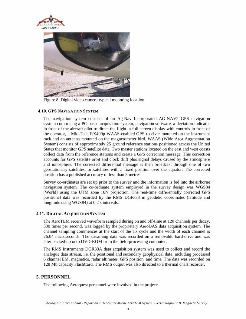
Figure 7. AeroTEM II Instrument Rack., including AeroDAS and RMS DGR-33 systems, AeroTEM power supply, data acquisition computer and AG-NAV2 navigation system.

4.7. MAGNETOMETER BASE STATION

The base magnetometer was a Geometrics G-859 cesium vapour magnetometer system with integrated GPS. Data logging and UTC time synchronisation was carried out within the magnetometer, with the GPS providing the timing signal. The data logging was configured to measure at 1.0 second intervals. Digital recording resolution was 0.001 nT. The sensor was placed on a tripod in an area of low magnetic gradient and free of cultural noise sources. A continuously updated display of the base station values was available for viewing and regularly monitored to ensure acceptable data quality and diurnal variation.

4.8. RADAR ALTIMETER

A Terra TRA 3500/TRI-30 radar altimeter is used to record terrain clearance. The antenna was mounted on the outside of the helicopter beneath the cockpit. Therefore, the recorded data reflect the height of the helicopter above the ground. The Terra altimeter has an altitude accuracy of +/- 1.5 metres.

4.9. VIDEO TRACKING AND RECORDING SYSTEM

A high resolution digital colour 8 mm video camera is used to record the helicopter ground flight path along the survey lines. The video is digitally annotated with GPS position and time and can be used to verify ground positioning information and cultural causes of anomalous geophysical responses.

Job # 08055


9

Figure 8. Digital video camera typical mounting location.

4.10. GPS NAVIGATION SYSTEM

The navigation system consists of an Ag-Nav Incorporated AG-NAV2 GPS navigation system comprising a PC-based acquisition system, navigation software, a deviation indicator in front of the aircraft pilot to direct the flight, a full screen display with controls in front of the operator, a Mid-Tech RX400p WAAS-enabled GPS receiver mounted on the instrument rack and an antenna mounted on the magnetometer bird. WAAS (Wide Area Augmentation System) consists of approximately 25 ground reference stations positioned across the United States that monitor GPS satellite data. Two master stations located on the east and west coasts collect data from the reference stations and create a GPS correction message. This correction accounts for GPS satellite orbit and clock drift plus signal delays caused by the atmosphere and ionosphere. The corrected differential message is then broadcast through one of two geostationary satellites, or satellites with a fixed position over the equator. The corrected position has a published accuracy of less than 3 metres.

Survey co-ordinates are set up prior to the survey and the information is fed into the airborne navigation system. The co-ordinate system employed in the survey design was WGS84 [World] using the UTM zone 16N projection. The real-time differentially corrected GPS positional data was recorded by the RMS DGR-33 in geodetic coordinates (latitude and longitude using WGS84) at 0.2 s intervals.

4.11. DIGITAL ACQUISITION SYSTEM

The AeroTEM received waveform sampled during on and off-time at 120 channels per decay, 300 times per second, was logged by the proprietary AeroDAS data acquisition system. The channel sampling commences at the start of the Tx cycle and the width of each channel is 26.04 microseconds. The streaming data was recorded on a removable hard-drive and was later backed-up onto DVD-ROM from the field-processing computer.

The RMS Instruments DGR33A data acquisition system was used to collect and record the analogue data stream, i.e. the positional and secondary geophysical data, including processed 6 channel EM, magnetics, radar altimeter, GPS position, and time. The data was recorded on 128 Mb capacity FlashCard. The RMS output was also directed to a thermal chart recorder.

5. PERSONNEL The following Aeroquest personnel were involved in the project:

Job # 08055


10

Manager of Operations: Bert Simon Manager of Data Processing: Gord Smith Field Data Processor: Geoff Plastow, Ali Latrous, Greg Roman Field Operator: Roberto Tito, Gab Genier Data Interpretation and Reporting: Alex Prikhodko, Marion Bishop

The survey pilot, Joel Reavie, was employed directly by the helicopter operator – Hi-Wood Helicopters.

6. DELIVERABLES

6.1. HARDCOPY DELIVERABLES

The report includes a set of four 1:20,000 maps. The survey area is covered by a single map plate and three geophysical data products are delivered as listed below:

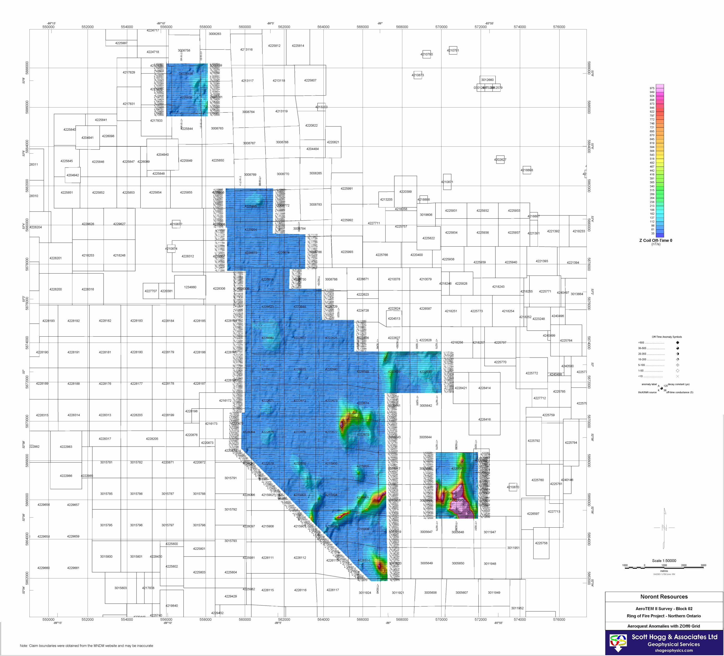
TMI – Coloured Total Magnetic Intensity (TMI) with line contours and EM anomaly symbols. ZOFF0 – AeroTEM Z0 Off-time with line contours and EM anomaly symbols. EM – AeroTEM off-time profiles Z1 – Z11 and EM anomaly symbols.

The coordinate/projection system for the maps is NAD83 – UTM Zone 16N. For reference, the latitude and longitude in WGS84 are also noted on the maps.

All the maps show flight path trace, skeletal topography, and conductor picks represented by an anomaly symbol classified according to calculated off-time conductance. The anomaly symbol is accompanied by postings denoting the calculated off-time conductance, a thick or thin classification and an anomaly identifier label. The anomaly symbol legend and survey specifications are displayed on the left margin of the maps.

6.2. DIGITAL DELIVERABLES

6.2.1. Final Database of Survey Data (.GDB, .XYZ)

The geophysical profile data is archived digitally in a Geosoft GDB binary format database. A description of the contents of the individual channels in the database can be found in Appendix 2. A copy of this digital data is archived at the Aeroquest head office in Mississauga.

6.2.2. Geosoft Grid files (.GRD)

Levelled Grid products used to generate the geophysical map images. Cell size for all grid files is 20 metres.

Total Magnetic Intensity from Mag sensor on the tow cable (MagU_TMI) Total Magnetic Intensity from Mag sensor on EM bird (MagL_TMI) AeroTEM Z Offtime Channel 1 (ZOFF0)

6.2.3. Digital Versions of Final Maps (.MAP, .PDF)

Map files in Geosoft .map and Adobe PDF format.

Job # 08055


11

6.2.4. Google Earth Survey Navigation Files (.KML)

Flight navigation lines in Google earth KML format. Double click to view flight lines in Google Earth.

6.2.5. Free Viewing Software (.EXE)

Geosoft Oasis Montaj Viewing Software Adobe Acrobat Reader Google Earth Viewer

6.2.6. Digital Copy of this Document (.PDF)

Adobe PDF format of this document.

7. DATA PROCESSING AND PRESENTATION All in-field and post-field data processing was carried out using Aeroquest proprietary data processing software and Geosoft Oasis Montaj software. Maps were generated using 36-inch wide Hewlett Packard ink-jet plotters.

7.1. BASE MAP

The geophysical maps accompanying this report are based on positioning in the NAD83 datum. The survey geodetic GPS positions have been projected using the Universal Transverse Mercator projection in Zone 16 North. A summary of the map datum and projection specifications is given following:

Ellipse: GRS 1980 Ellipse major axis: 6378137m eccentricity: 0.081819191 Datum: North American 1983 - Canada Mean Datum Shifts (x,y,z) : 0, 0, 0 metres Map Projection: Universal Transverse Mercator Zone 16 (Central Meridian 87ºW) Central Scale Factor: 0.9996 False Easting, Northing: 500,000m, 0m

For reference, the latitude and longitude in WGS84 are also noted on the maps.

The background vector topography derived from Natural Resources Canada 1:50000 National Topographic Data Base data and the background shading was derived from NASA Shuttle Radar Topography Mission (SRTM) 90 metre resolution DEM data.

7.2. FLIGHT PATH & TERRAIN CLEARANCE

The position of the survey helicopter was directed by use of the Global Positioning System (GPS). Positions were updated five times per second (5 Hz) and expressed as WGS84 latitude and longitude calculated from the raw pseudo range derived from the C/A code signal. The instantaneous GPS flight path, after conversion to UTM co-ordinates, is drawn using linear interpolation between the x/y positions. The terrain clearance was maintained with reference to the radar altimeter. The raw Digital Terrain Model (DTM) was derived by taking the GPS survey elevation and subtracting the radar altimeter terrain clearance values. The calculated topography elevation values are relative and are not tied in to surveyed geodetic heights.

Job # 08055


12

Each flight included at least two high elevation ‘background’ checks. These high elevation checks are to ensure that the gain of the system remained constant and within specifications.

7.3. ELECTROMAGNETIC DATA

The raw streaming data, sampled at a rate of 36,000 Hz (120 channels, 300 times per second) was reprocessed using a proprietary software algorithm developed and owned by Aeroquest Limited. Processing involves the compensation of the X and Z component data for the primary field waveform. Coefficients for this compensation for the system transient are determined and applied to the stream data. The stream data are then pre-filtered, stacked, binned to the 33 on and off-time channels and checked for the effectiveness of the compensation and stacking processes. The stacked data is then filtered, levelled and split up into the individual line segments. Further base level adjustments may be carried out at this stage. The filtering of the stacked data is designed to remove or minimize high frequency noise that can not be sourced from the geology.

The final field processing step was to merge the processed EM data with the other data sets into a Geosoft GDB file. The EM fiducial is used to synchronize the two datasets. The processed channels are merged into ‘array format; channels in the final Geosoft database as Zon, Zoff, Xon, and Xoff.

Apparent bedrock EM anomalies were interpreted with the aid of an auto-pick from positive peaks and troughs in the off-time Z channel responses correlated with X channel responses. The auto-picked anomalies were reviewed and edited by a geophysicist on a line by line basis to discriminate between thin and thick conductor types. Anomaly picks locations were migrated and removed as required. This process ensures the optimal representation of the conductor centres on the maps.

At each conductor pick, estimates of the off-time conductance have been generated based on a horizontal plate source model for those data points along the line where the response amplitude is sufficient to yield an acceptable estimate. Some of the EM anomaly picks do not display a Tau value; this is due to the inability to properly define the decay of the conductor usually because of low signal amplitudes. Each conductor pick was then classified according to a set of seven ranges of calculated off-time conductance values. For high conductance sources, the on-time conductance values may be used, since it provides a more accurate measure of high-conductance sources. Each symbol is also given an identification letter label, unique to each flight line. Conductor picks that did not yield an acceptable estimate of off-time conductance due to a low amplitude response were classified as a low conductance source. Please refer to the anomaly symbol legend located in the margin of the maps.

7.4. MAGNETIC DATA

Prior to any levelling the magnetic data was subjected to a lag correction of -0.1 seconds and a spike removal filter. The filtered aeromagnetic data were then corrected for diurnal variations using the magnetic base station and the intersections of the tie lines. No corrections for the regional reference field (IGRF) were applied. The corrected profile data were interpolated on to a grid using a bi-directional grid technique with a grid cell size of 20 metres. The final levelled grid provided the basis for threading the presented contours which have a minimum contour interval of 50 nT.

Job # 08055


13

8. GENERAL COMMENTS The survey was successful in mapping the magnetic and conductive properties of the geology throughout the survey area. Below is a brief interpretation of the results. For a detailed interpretation please contact Aeroquest Limited.

8.1. MAGNETIC RESPONSE

The magnetic data provide a high resolution map of the distribution of the magnetic mineral content of the survey area. This data can be used to interpret the location of geological contacts and other structural features such as faults and zones of magnetic alteration. The sources for anomalous magnetic responses are generally thought to be predominantly magnetite because of the relative abundance and strength of response (high magnetic susceptibility) of magnetite over other magnetic minerals such as pyrrhotite.

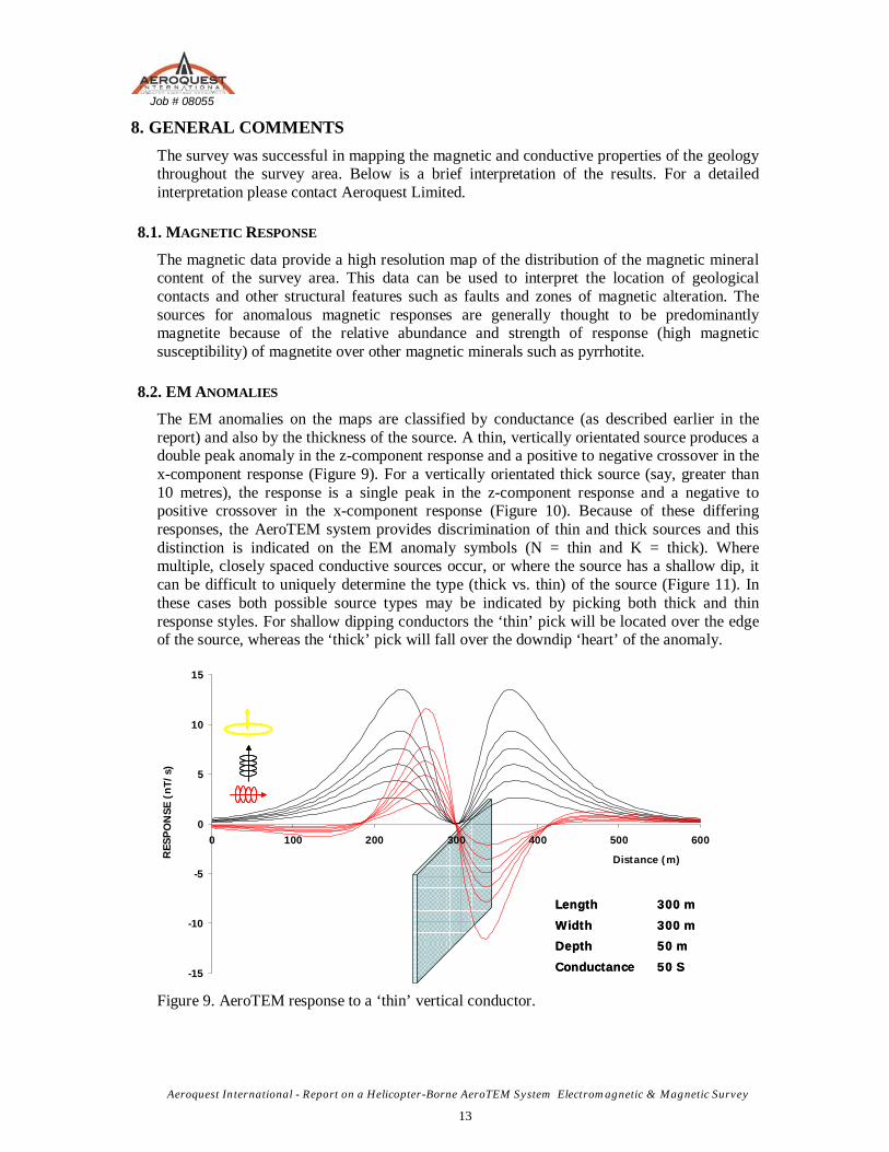
8.2. EM ANOMALIES

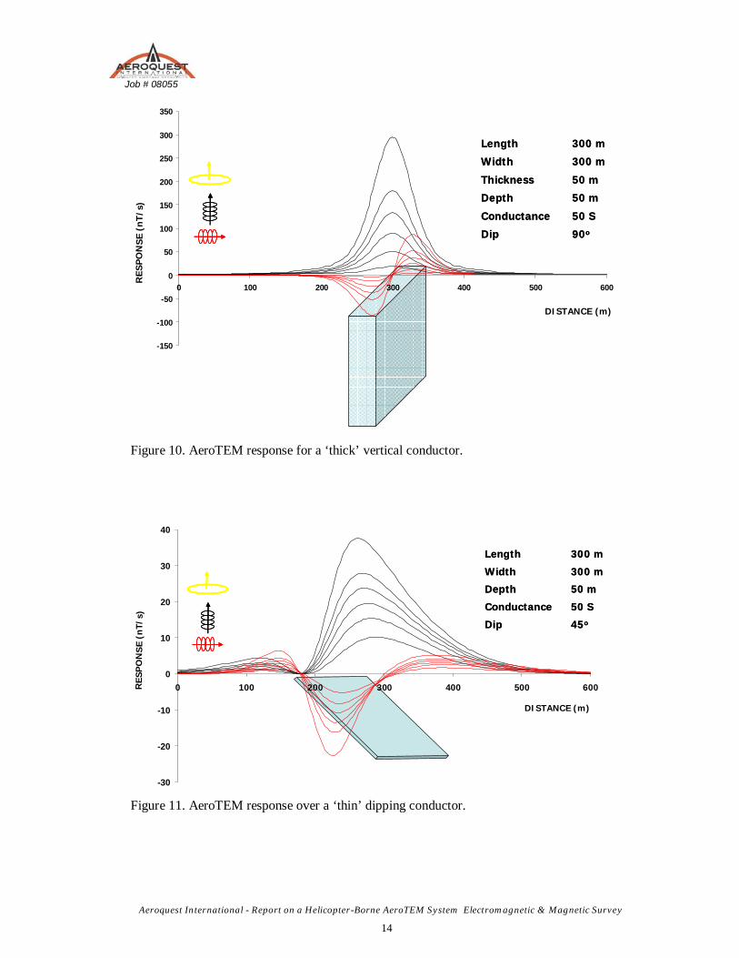
The EM anomalies on the maps are classified by conductance (as described earlier in the report) and also by the thickness of the source. A thin, vertically orientated source produces a double peak anomaly in the z-component response and a positive to negative crossover in the x-component response (Figure 9). For a vertically orientated thick source (say, greater than 10 metres), the response is a single peak in the z-component response and a negative to positive crossover in the x-component response (Figure 10). Because of these differing responses, the AeroTEM system provides discrimination of thin and thick sources and this distinction is indicated on the EM anomaly symbols (N = thin and K = thick). Where multiple, closely spaced conductive sources occur, or where the source has a shallow dip, it can be difficult to uniquely determine the type (thick vs. thin) of the source (Figure 11). In these cases both possible source types may be indicated by picking both thick and thin response styles. For shallow dipping conductors the ‘thin’ pick will be located over the edge of the source, whereas the ‘thick’ pick will fall over the downdip ‘heart’ of the anomaly.

-15

-10

-5

0

5

10

15

0 100 200 300 400 500 600

50 SConductance

50 mDepth

300 mWidth

300 mLength

50 SConductance

50 mDepth

300 mWidth

300 mLength

Distance (m)RES

PO

NSE

(n T

/s)

Figure 9. AeroTEM response to a ‘thin’ vertical conductor.

Job # 08055


14

-150

-100

-50

0

50

100

150

200

250

300

350

0 100 200 300 400 500 600

50 SConductance

50 mDepth

50 mThickness

90oDip

300 mWidth

300 mLength

50 SConductance

50 mDepth

50 mThickness

90oDip

300 mWidth

300 mLength

DISTANCE (m)

RE

SP

ON

SE

(nT

/s)

Figure 10. AeroTEM response for a ‘thick’ vertical conductor.

-30

-20

-10

0

10

20

30

40

0 100 200 300 400 500 600

50 SConductance

45oDip

50 mDepth

300 mWidth

300 mLength

50 SConductance

45oDip

50 mDepth

300 mWidth

300 mLength

DISTANCE (m)

RES

PO

NS

E (n

T/s)

Figure 11. AeroTEM response over a ‘thin’ dipping conductor.

Job # 08055


15

All cases should be considered when analyzing the interpreted picks and prioritizing for follow-up. Specific anomalous responses which remain as high priority should be subjected to numerical modeling prior to drill testing to determine the dip, depth and probable geometry of the source.

Respectfully submitted,

Dr. Alex Prikhodko PhD Geophysicist Aeroquest Limited February 2008

Reviewed By:

Doug Garrie Aeroquest Limited February 2008

Job # 08055


6

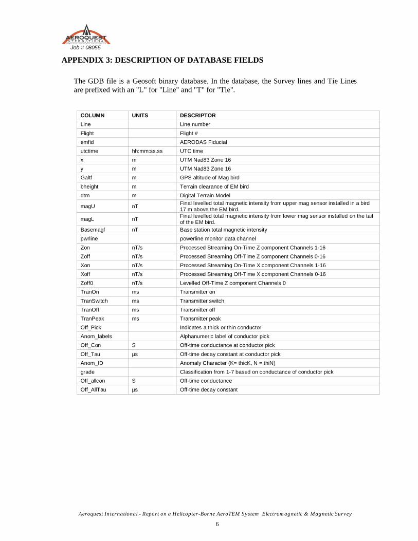
APPENDIX 3: DESCRIPTION OF DATABASE FIELDS

The GDB file is a Geosoft binary database. In the database, the Survey lines and Tie Lines are prefixed with an "L" for "Line" and "T" for "Tie".

COLUMN UNITS DESCRIPTOR Line Line number

Flight Flight # emfid AERODAS Fiducial utctime hh:mm:ss.ss UTC time x m UTM Nad83 Zone 16 y m UTM Nad83 Zone 16 Galtf m GPS altitude of Mag bird

bheight m Terrain clearance of EM bird dtm m Digital Terrain Model

magU nT Final levelled total magnetic intensity from upper mag sensor installed in a bird 17 m above the EM bird.

magL nT Final levelled total magnetic intensity from lower mag sensor installed on the tail of the EM bird.

Basemagf nT Base station total magnetic intensity pwrline powerline monitor data channel

Zon nT/s Processed Streaming On-Time Z component Channels 1-16 Zoff nT/s Processed Streaming Off-Time Z component Channels 0-16 Xon nT/s Processed Streaming On-Time X component Channels 1-16 Xoff nT/s Processed Streaming Off-Time X component Channels 0-16 Zoff0 nT/s Levelled Off-Time Z component Channels 0 TranOn ms Transmitter on

TranSwitch ms Transmitter switch TranOff ms Transmitter off TranPeak ms Transmitter peak Off_Pick Indicates a thick or thin conductor Anom_labels Alphanumeric label of conductor pick Off_Con S Off-time conductance at conductor pick

Off_Tau µs Off-time decay constant at conductor pick Anom_ID Anomaly Character (K= thicK, N = thiN) grade Classification from 1-7 based on conductance of conductor pick Off_allcon S Off-time conductance Off_AllTau µs Off-time decay constant

Job # 08055


10

APPENDIX 5: AEROTEM DESIGN CONSIDERATIONS

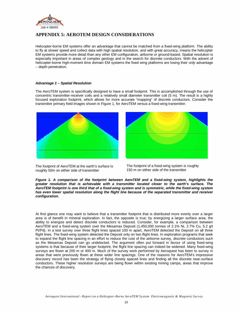
Helicopter-borne EM systems offer an advantage that cannot be matched from a fixed-wing platform. The ability to fly at slower speed and collect data with high spatial resolution, and with great accuracy, means the helicopter EM systems provide more detail than any other EM configuration, airborne or ground-based. Spatial resolution is especially important in areas of complex geology and in the search for discrete conductors. With the advent of helicopter-borne high-moment time domain EM systems the fixed wing platforms are losing their only advantage – depth penetration.

Advantage 1 – Spatial Resolution

The AeroTEM system is specifically designed to have a small footprint. This is accomplished through the use of concentric transmitter-receiver coils and a relatively small diameter transmitter coil (5 m). The result is a highly focused exploration footprint, which allows for more accurate “mapping” of discrete conductors. Consider the transmitter primary field images shown in Figure 1, for AeroTEM versus a fixed-wing transmitter.

The footprint of AeroTEM at the earth’s surface is roughly 50m on either side of transmitter Figure 1. A comparison of the footprint between AeroTEM and a fixed-wing system, highlights the greater resolution that is achievable with a transmitter located closer to the earth’s surface. The AeroTEM footprint is one third that of a fixed-wing system and is symmetric, while the fixed-wing system has even lower spatial resolution along the flight line because of the separated transmitter and receiver configuration.

At first glance one may want to believe that a transmitter footprint that is distributed more evenly over a larger area is of benefit in mineral exploration. In fact, the opposite is true; by energizing a larger surface area, the ability to energize and detect discrete conductors is reduced. Consider, for example, a comparison between AeroTEM and a fixed-wing system over the Mesamax Deposit (1,450,000 tonnes of 2.1% Ni, 2.7% Cu, 5.2 g/t Pt/Pd). In a test survey over three flight lines spaced 100 m apart, AeroTEM detected the Deposit on all three flight lines. The fixed-wing system detected the Deposit only on two flight lines. In exploration programs that seek to expand the flight line spacing in an effort to reduce the cost of the airborne survey, discrete conductors such as the Mesamax Deposit can go undetected. The argument often put forward in favour of using fixed-wing systems is that because of their larger footprint, the flight line spacing can indeed be widened. Many fixed-wing surveys are flown at 200 m or 400 m. Much of the survey work performed by Aeroquest has been to survey in areas that were previously flown at these wider line spacings. One of the reasons for AeroTEM’s impressive discovery record has been the strategy of flying closely spaced lines and finding all the discrete near-surface conductors. These higher resolution surveys are being flown within existing mining camps, areas that improve the chances of discovery.

The footprint of a fixed-wing system is roughly 150 m on either side of the transmitter

Job # 08055


11

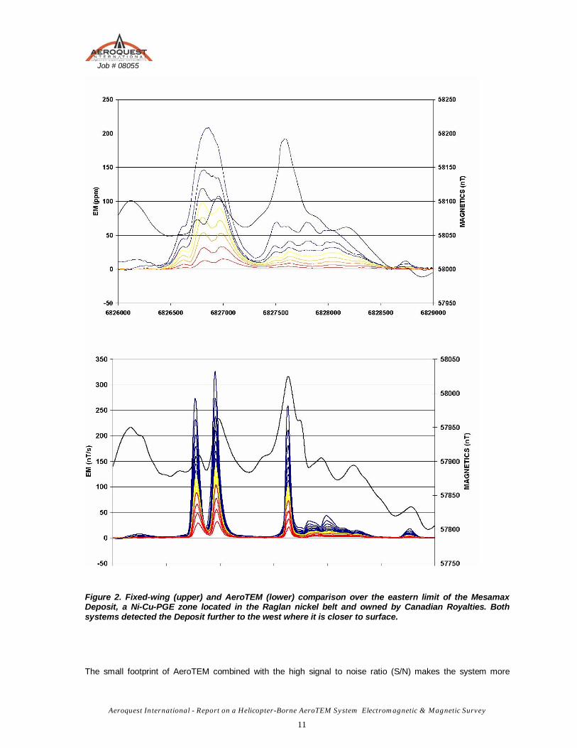
Figure 2. Fixed-wing (upper) and AeroTEM (lower) comparison over the eastern limit of the Mesamax Deposit, a Ni-Cu-PGE zone located in the Raglan nickel belt and owned by Canadian Royalties. Both systems detected the Deposit further to the west where it is closer to surface.

The small footprint of AeroTEM combined with the high signal to noise ratio (S/N) makes the system more

Job # 08055


12

suitable to surveying in areas where local infrastructure produces electromagnetic noise, such as power lines and railways. In 2002 Aeroquest flew four exploration properties in the Sudbury Basin that were under option by FNX Mining Company Inc. from Inco Limited. One such property, the Victoria Property, contained three major power line corridors.

The resulting AeroTEM survey identified all the known zones of Ni-Cu-PGE mineralization, and detected a response between two of the major power line corridors but in an area of favorable geology. Three boreholes were drilled to test the anomaly, and all three intersected sulphide. The third borehole encountered 1.3% Ni, 6.7% Cu, and 13.3 g/t TPMs over 42.3 ft. The mineralization was subsequently named the Powerline Deposit.

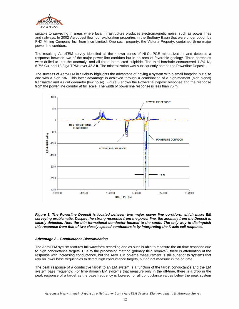
The success of AeroTEM in Sudbury highlights the advantage of having a system with a small footprint, but also one with a high S/N. This latter advantage is achieved through a combination of a high-moment (high signal) transmitter and a rigid geometry (low noise). Figure 3 shows the Powerline Deposit response and the response from the power line corridor at full scale. The width of power line response is less than 75 m.

Figure 3. The Powerline Deposit is located between two major power line corridors, which make EM surveying problematic. Despite the strong response from the power line, the anomaly from the Deposit is clearly detected. Note the thin formational conductor located to the south. The only way to distinguish this response from that of two closely spaced conductors is by interpreting the X-axis coil response.

Advantage 2 – Conductance Discrimination

The AeroTEM system features full waveform recording and as such is able to measure the on-time response due to high conductance targets. Due to the processing method (primary field removal), there is attenuation of the response with increasing conductance, but the AeroTEM on-time measurement is still superior to systems that rely on lower base frequencies to detect high conductance targets, but do not measure in the on-time.

The peak response of a conductive target to an EM system is a function of the target conductance and the EM system base frequency. For time domain EM systems that measure only in the off-time, there is a drop in the peak response of a target as the base frequency is lowered for all conductance values below the peak system

Job # 08055


13

response. For example, the AeroTEM peak response occurs for a 10 S conductor in the early off-time and 100 S in the late off-time for a 150 Hz base frequency. Because base frequency and conductance form a linear relationship when considering the peak response of any EM system, a drop in base frequency of 50% will double the conductance at which an EM system shows its peak response. If the base frequency were lowered from 150 Hz to 30 Hz there would be a fivefold increase in conductance at which the peak response of an EM occurred.

However, in the search for highly conductive targets, such as pyrrhotite-related Ni-Cu-PGM deposits, a fivefold increase in conductance range is a high price to pay because the signal level to lower conductance targets is reduced by the same factor of five. For this reason, EM systems that operate with low base frequencies are not suitable for general exploration unless the target conductance is more than 100 S, or the target is covered by conductive overburden.

Despite the excellent progress that has been made in modeling software over the past two decades, there has been little work done on determining the optimum form of an EM system for mineral exploration. For example, the optimum configuration in terms of geometry, base frequency and so remain unknown. Many geophysicists would argue that there is no single ideal configuration, and that each system has its advantages and disadvantages. We disagree.

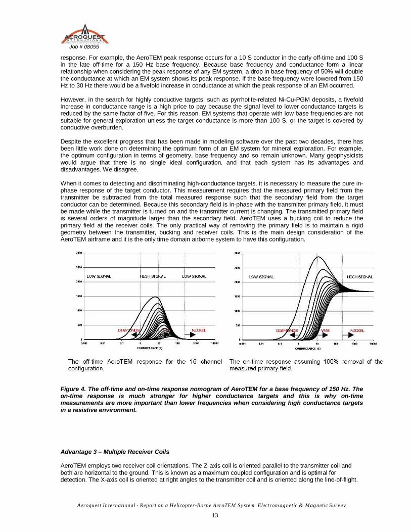
When it comes to detecting and discriminating high-conductance targets, it is necessary to measure the pure in-phase response of the target conductor. This measurement requires that the measured primary field from the transmitter be subtracted from the total measured response such that the secondary field from the target conductor can be determined. Because this secondary field is in-phase with the transmitter primary field, it must be made while the transmitter is turned on and the transmitter current is changing. The transmitted primary field is several orders of magnitude larger than the secondary field. AeroTEM uses a bucking coil to reduce the primary field at the receiver coils. The only practical way of removing the primary field is to maintain a rigid geometry between the transmitter, bucking and receiver coils. This is the main design consideration of the AeroTEM airframe and it is the only time domain airborne system to have this configuration.

Figure 4. The off-time and on-time response nomogram of AeroTEM for a base frequency of 150 Hz. The on-time response is much stronger for higher conductance targets and this is why on-time measurements are more important than lower frequencies when considering high conductance targets in a resistive environment.

Advantage 3 – Multiple Receiver Coils

AeroTEM employs two receiver coil orientations. The Z-axis coil is oriented parallel to the transmitter coil and both are horizontal to the ground. This is known as a maximum coupled configuration and is optimal for detection. The X-axis coil is oriented at right angles to the transmitter coil and is oriented along the line-of-flight.

Job # 08055


14

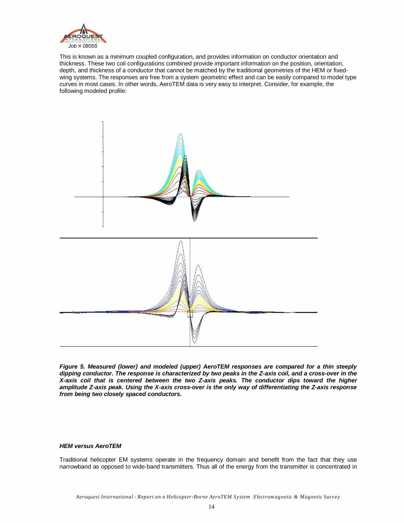
This is known as a minimum coupled configuration, and provides information on conductor orientation and thickness. These two coil configurations combined provide important information on the position, orientation, depth, and thickness of a conductor that cannot be matched by the traditional geometries of the HEM or fixed-wing systems. The responses are free from a system geometric effect and can be easily compared to model type curves in most cases. In other words, AeroTEM data is very easy to interpret. Consider, for example, the following modeled profile:

Figure 5. Measured (lower) and modeled (upper) AeroTEM responses are compared for a thin steeply dipping conductor. The response is characterized by two peaks in the Z-axis coil, and a cross-over in the X-axis coil that is centered between the two Z-axis peaks. The conductor dips toward the higher amplitude Z-axis peak. Using the X-axis cross-over is the only way of differentiating the Z-axis response from being two closely spaced conductors.

HEM versus AeroTEM

Traditional helicopter EM systems operate in the frequency domain and benefit from the fact that they use narrowband as opposed to wide-band transmitters. Thus all of the energy from the transmitter is concentrated in

Job # 08055


15

a few discrete frequencies. This allows the systems to achieve excellent depth penetration (up to 100 m) from a transmitter of modest power. The Aeroquest Impulse system is one implementation of this technology.

The AeroTEM system uses a wide-band transmitter and delivers more power over a wide frequency range. This frequency range is then captured into 16 time channels, the early channels containing the high frequency information and the late time channels containing the low frequency information down to the system base frequency. Because frequency domain HEM systems employ two coil configurations (coplanar and coaxial) there are only a maximum of three comparable frequencies per configuration, compared to 16 AeroTEM off-time and 12 AeroTEM on-time channels.

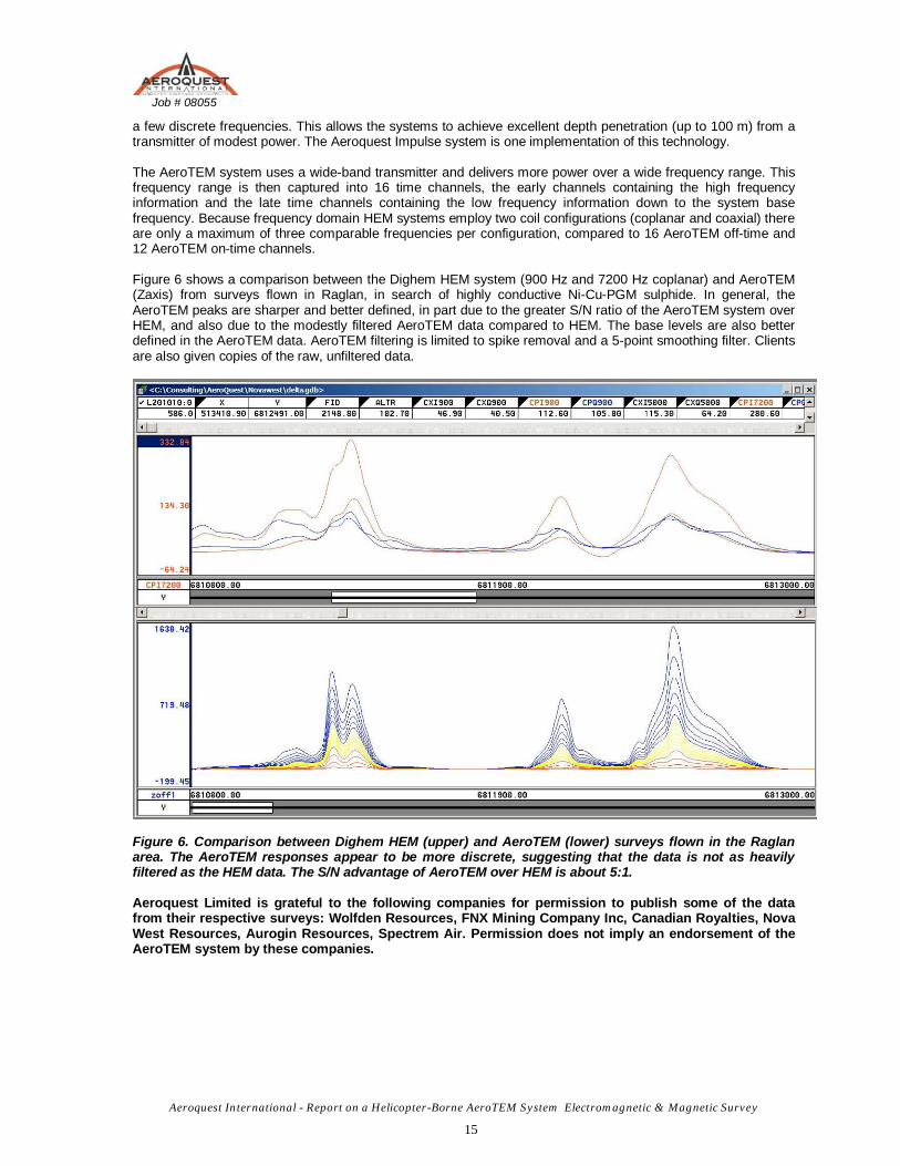
Figure 6 shows a comparison between the Dighem HEM system (900 Hz and 7200 Hz coplanar) and AeroTEM (Zaxis) from surveys flown in Raglan, in search of highly conductive Ni-Cu-PGM sulphide. In general, the AeroTEM peaks are sharper and better defined, in part due to the greater S/N ratio of the AeroTEM system over HEM, and also due to the modestly filtered AeroTEM data compared to HEM. The base levels are also better defined in the AeroTEM data. AeroTEM filtering is limited to spike removal and a 5-point smoothing filter. Clients are also given copies of the raw, unfiltered data.

Figure 6. Comparison between Dighem HEM (upper) and AeroTEM (lower) surveys flown in the Raglan area. The AeroTEM responses appear to be more discrete, suggesting that the data is not as heavily filtered as the HEM data. The S/N advantage of AeroTEM over HEM is about 5:1.

Aeroquest Limited is grateful to the following companies for permission to publish some of the data from their respective surveys: Wolfden Resources, FNX Mining Company Inc, Canadian Royalties, Nova West Resources, Aurogin Resources, Spectrem Air. Permission does not imply an endorsement of the AeroTEM system by these companies.

Job # 08055


16

APPENDIX 6: AEROTEM INSTRUMENTATION SPECIFICATION SHEET

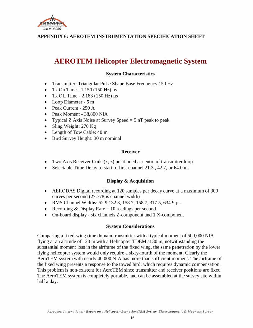
AEROTEM Helicopter Electromagnetic System

System Characteristics

• Transmitter: Triangular Pulse Shape Base Frequency 150 Hz • Tx On Time - 1,150 (150 Hz) µs • Tx Off Time - 2,183 (150 Hz) µs • Loop Diameter - 5 m • Peak Current - 250 A • Peak Moment - 38,800 NIA • Typical Z Axis Noise at Survey Speed = 5 nT peak to peak • Sling Weight: 270 Kg • Length of Tow Cable: 40 m • Bird Survey Height: 30 m nominal

Receiver

• Two Axis Receiver Coils (x, z) positioned at centre of transmitter loop • Selectable Time Delay to start of first channel 21.3 , 42.7, or 64.0 ms

Display & Acquisition

• AERODAS Digital recording at 120 samples per decay curve at a maximum of 300 curves per second (27.778µs channel width)

• RMS Channel Widths: 52.9,132.3, 158.7, 158.7, 317.5, 634.9 µs • Recording & Display Rate = 10 readings per second. • On-board display - six channels Z-component and 1 X-component

System Considerations

Comparing a fixed-wing time domain transmitter with a typical moment of 500,000 NIA flying at an altitude of 120 m with a Helicopter TDEM at 30 m, notwithstanding the substantial moment loss in the airframe of the fixed wing, the same penetration by the lower flying helicopter system would only require a sixty-fourth of the moment. Clearly the AeroTEM system with nearly 40,000 NIA has more than sufficient moment. The airframe of the fixed wing presents a response to the towed bird, which requires dynamic compensation. This problem is non-existent for AeroTEM since transmitter and receiver positions are fixed. The AeroTEM system is completely portable, and can be assembled at the survey site within half a day.

-86'15'

550000 I

552000 554000 _86'10'

556000 4LL41 1 I I

4224718

o o o ~~------r----------------r----------~----r-----r---~E~\~§i~g co ,L 'OL~

o o o (fJ IX]

tB

,on.ln. 1

4225841 4217833

4226098

3Q08758 j

'" ,. o

j

'" ,. 11225844

558000

3008263

3008763

_86'5'

560000 562000

4225812 42' 3116

"I)UOlb4 42131 9

4225814

564000

.C [

4220822

_86'

566000 568000 570000 I

_85'55'

572000 I

574000 576000

Ul en en m o 8

o Ul

O~====~-t-1=========t~==t====f------+----t----~-1--------r----f=========f=P====~=====r---1~UUO~11~'OI __ -1 ____ ~"U~UOI~OO ____ +--'~4<W~11~4~22=0~8~2~1t-______ -1 ________________ +----------------1----------------+---------------------------------+---------~en~ ~ ~~ _ ~ 4204484 8 ~ ~ L() 0 Ol -

4225845 4225846 I( 4225849 4225850 28311

~--~4204942~_r----------~----r_--~--~--42-2-5-84-8_r~------------+_r_--------~,

4225851 4225852 4225854 4225855

"uue'lu 3008265

4225991

"'J~ ,~\ ~( 4: P ""-----1 4225931 4225933

4213205

3008783

Ul en en " o o o

H~i~ ~ 3019606 4 ~1 uRuR,O;-----t--,------1 - 4225992 f---+-----------+-----+------+------------.:.rc- - g: ~

~1·~~30~~=78~4----~-+--------4-~~11-+--~4220~i5~)~7--~====~~----~--~----~--------+-~-----+--+---~~

o o o IX]

"IX] co

fJo _ ">0 "'0

(fJ

"IX] co

o o o N "IX] co

o o

4228201

4228200

4228192

4228191

4228314

421 ,253 4218248

422,316

4228182

4228181

4228313

4228312

1234660

I

4228183 42:'8184 4228185

4228180 42:'8179 4228186

4:2:2B1! (

42211198 4228203

4228306

~, ~'

~~ 4216172 k

~j-------t---t------------H-------------t--t---------II-----t------1===t==t~t42~161~7~3~t--~Sl co ~l

8 o co (fJ co co

o o o (fJ (fJ IX] co

= 4222983

4222986

4229657

I 550000 552000

_86'15'

4228317 4228205

3015781 3015782

3015785 3015786

3015795 3015796

3015800 3015801

3015802 42178:18

554000

Note. Claim boundaries were obtained from the MNDM website and may be inaccurate

OU 0101

1219840

556000 _86' 10'

4220876 t

3015788

3015798

558000

~ H~~~ ': ;2190

t\o ' L\

3015791

3015792

4229429

<!.l<Ji

qrtt'~ i: <1:1~~~

4215906

4226115

560000

~~. 0 <L 10 4225934 4225937 4~213~ 1 422139; 4218233

<I

I 562000

_86'S'

!D 4225822

4225993 4225766 4220400

3008788 42215671 4210078 4210079

4225938 4221393

4218243 'Qcb, 4225771

4221394 Ul en --.j en o o o

Ul en --.j

~----+------r----~----------~-+--------------1--------+--------~----1-------------~,T~~~~~~~~~l~~~1t~t~~~~~~~~§0 . 4222624 4226587 ~. 4218251 4LLO, 4218254

..

4226116 4226117 30 1924

564000 566000

4204513 ,~ 'v~ 4223248

~~--~--r-------~----~--_,--~~------~~

4225770

4225772

~~. ml4228421 4228414

4227712

4LLpiOO

-

4LLOI

u, en --.j

" o

f-------18

42257!

4225794

g: ~--------------+_-----+------__1_+_----_+----1~

o o o

30119:11

568000 _86'

~ ~ ~

3005647 ~ 3011947

~----------~--+_-----------1 3011951

3005649 3005650 3011948

3005606 3005607 3011949

3011952

I 570000 572000 574000

_85'55'

4225760

4226597

4225758

422771

1

576000

-

Ul en m m o o o

Ul en m El 8

~ ~

'"

1000 IiiiiiiiiiiI

19.5 19.0 18.5 17.9 17.4

16.9 16.4

15.9

15.4

14.9 14.4

13.B

13.3 12.8 12.3 11.8 11.3

10.8

10.3

9.7 9.2 8.7 8.2 7.7

7.2 6.7

6.2 5.6

5.1

4.6 4.1

3.6 3.1

26 21 15

1.0 0.5

Conductance (Siemens)

Interpretation Legend

OEM response location Unless referenced with a conductor axis and report number, it is considered to be associated with overburden conductivity

~ Conductor axis with report reference

-- Zone of high conductivity

Fault

Profile Scale. 4 Siemens / mm

a Scale 1 :50000

1000

metres N!-.o83IUTM zone 16N

2000

Noront Resources

3000

AeroTEM II Survey - Block 02

Ring of Fire Project - Northern Ontario

Interpretation with Conductance

o

-86'15'

550000 I

552000 554000 _86'10'

556000 4LL41 I I I

4224718

8 ~ ~~------r----------------r----------~----r-----r---~E~\~§i~g __ co ,L 'OL~

- r -

4225841 4217833

,on.ln. 1 4226098

3Q08758 j

'" ,. o

j

'" ,. 11225844

_86'5'

558000 560000 562000

3008263

4225812 4225814 42" 3116

4220822 3008763

_86'

564000 566000 568000 I

570000 _85'55'

572000 I

574000 576000

o Ul

D~====~-t-1=========t~==t====f------+----t----~-1--------r----f=========f=P====~=====r---1~UU~~11~,ol __ -1 ____ ~ou~uol~oo ____ +--'~4<W~11~4~22=0~8~2~1t-______ -1 ________________ +----------------1----------------+---------------------------------+---------~00~ ~ ~~ _ ~ 4204484 8 ~ ~ L() 0 Ol -

4225845 4225846 I( 4225849 4225850 28311

~--~4204942~_r----------~----r_--~--~--42-2-5-84-8_r~------------+_r_--------~,

o o o '" '" '" co

o o o N

'" '" co

o o o <D <D

'" co

=

4228201

4228200

4228192

4228314

4222983

4222986

4229657

4229659

4229661

I 550000

_86'15'

421 ,253 4218248

422,316

4228182 4228183

4:2:2B1! (

4228313 4228203

3015781 3015782

3015785 3015786

3015795 3015796

3015800 3015801

3015803 42178:18

552000 554000

Note: Claim boundaries were obtained from the MNDM website and may be inaccurate

1219840

556000 _86' 10'

4228312

1234660

4221:198

4LLUOIL

3015788

3015798

4225801

558000

4228306

3015791

3015792

3015793

4229429

OUUC'IU

4215906

4226111

4226115

I 560000 562000

_86'S'

4225993

4226112 42261

4226116 4226117 30 1924

564000 566000

4225766 4220400

~ j ~ ~ ~ ~

g 3005642 ;3

:'\- <L 12550

j ~ ~ ~

3005647 ~

4225938

4225770

4228414

4228416

3011947

4221393

,~ 'v~ 4223248

4225772

4LLpiOO

4227712

4225759 1----

4225760

4226597 422771

4225758 ~----------~--+_--------___1 3011951

3005649 3005650 3011948

3005606 3005607 3011949

3011952

I 1

568000 570000 572000 574000 576000 _86' _85'55'

4221394

-

4LLOI

Ul 00 --.j 00 o o o

U' 00 --.j

" o

1------18

42257!

-

Ul 00 OJ OJ o o o

Ul 00 OJ

El 8

~ ~

'"

1000 IiiiiiiiiiiI

1.93 1.00 0.73

0.56 0.44

0.34

0.27

0.20

0.14

0.08

0.03

-0.00

-0.03

-0.05

-0.D7

-0.08

-0.09 -0.10

-0.11

-0.12

-0.13

-0.14

-0.16

-0.18

-0.20

-0.23

-0.25

-0.29

-0.33

-0.37

-0.42

-0.47

-0.53

-061

-071

-OB7

-1.13 -1.74

Vertical Derivative (nTlm)




-- Zone of high conductiVity

o

Fault

Scale 1 :50000 1000


2000

Noront Resources

3000



Interpretation with Calculated Vertical Derivative (Reduced to Pole)

-86'15'

550000 I

552000 554000 _86'10'

556000 4LL41 I I I

4224718

o o o ~~------r----------------r----------~----r-----r---~E~\~§i~g co ,L 'OL~

o o o (fJ aJ

tB

,on.ln. 1

4225841 4217833

4226098

3Q08758 j

'" ,. o

j

'" ,. 11225844

558000

3008263

0-- ~ ,~ L i

~ ~~ ; 1-~---1 3008763

_86'S'

560000 562000

4225812 42' 3116

42 3117 421311

"I)UOlb4 42131 9

4225814

564000

4225807

.C [

4220822

_86'

566000 568000 570000 I

_85'55'

572000 I

574000 576000

Ul

Ul en en m o 8

o Ul

O~====~-t-1=========t~==t====f------+----t----~-1--------r----f=========f=P====~=====r---1~UUO~11~'OI __ -1 ____ ~"U~UOI~OO ____ +--'~4<W~11~4~22=0~8~2~1t-______ -1 ________________ +----------------1----------------+---------------------------------+---------~en~ ~ ~~ _ ~ 4204484 8 ~ ~ L() 0 Ol -

4225845 4225846 I( 4225849 4225850 28311

~--~4204942~_r----------~----r_--~--~--42-2-5-84-8_r~------------+_r_--------~,

o o o aJ

"" aJ co

fJo _ ">0 "'0

(fJ

"" aJ co

o o o N "aJ co

o o o (fJ (fJ aJ co

=

4228201

4228200

4228192

4228191

4228314

4222983

4222986

4229657

4229659

4229661

I 550000

_86'15'

421 ,253 4218248

422,316

4228182 4228183

4228181 4228180

4:2:2B1! (

4228313 4228203

4228317 4228205

3015785 3015786

3015795 3015796

3015800 3015801

3015803 42178:18

552000 554000


42:'8184

42:'8179

OU 0101

OU 01~1

1219840

556000 _86' 10'

4228312

1234660

I

4228185

4228186

4221:198

3015788

3015798

4225801

558000

4228306

~~ 4216172 k

3015791

3015792

3015793

4229429

"uue'lu

4215906

4226111

4226115

I 560000 562000

_86'S'

4226112

4226116

4225993 4225766 4220400

3008788 42215671 4210078 4210079

4225938 4221393

4218243 'Qcb, 4225771

4221394 Ul en --.j en o o o

Ul en --.j

~----+------r----~----------~-+-------------r-------+--------~---r------------~,T~~~~~~~~~l~~~1t~t~~~~~~~~§0 . 4222624 4226587 ~. 4218251 4LLO, 4218254

42261

4226117 30 1924

564000 566000

4204513 ,~ 'v~ 4223248

~~--~--r-------~----~--_,--~~------~~

4225770

4225772

4228414

~ j 4227712 ~ ~ ~ ~

g 3005642 ;3

4LLpiOO

-

4LLOI

u, en --.j

" o

1------18

42257!

g: ~--------------+_----_+------_r+_----_+~~

o o o

568000 _86'

j ~ ~ ~

3005647 ~ 3011947

~----------~--+_--------___1 3011951

3005649 3005650 3011948

3005606 3005607 3011949

3011952

I 570000 572000 574000

_85'55'

4225760

4226597

4225758

422771

1

576000

-

Ul en m m o o o

Ul en m El 8

~ ~

'"

1000 IiiiiiiiiiiI

AeroTEM Profiles

positive excursion to top and right, 1 mm=25nT/s

Z4 Off-Time Channel Z5 Off-Time Channel Z6 Off-Time Channel Z8 Off-Time Channel Z10 Off-Time Channel Z11 Off-Time Channel Z12 Off-Time Channel Z13 Off-Time Channel Z13 Off-Time Channel Z14 Off-Time Channel Z15 Off-Time Channel





o

Fault

Scale 1 :50000 1000


2000

Noront Resources

3000



Interpretation with Z Coil Off-Time Profiles

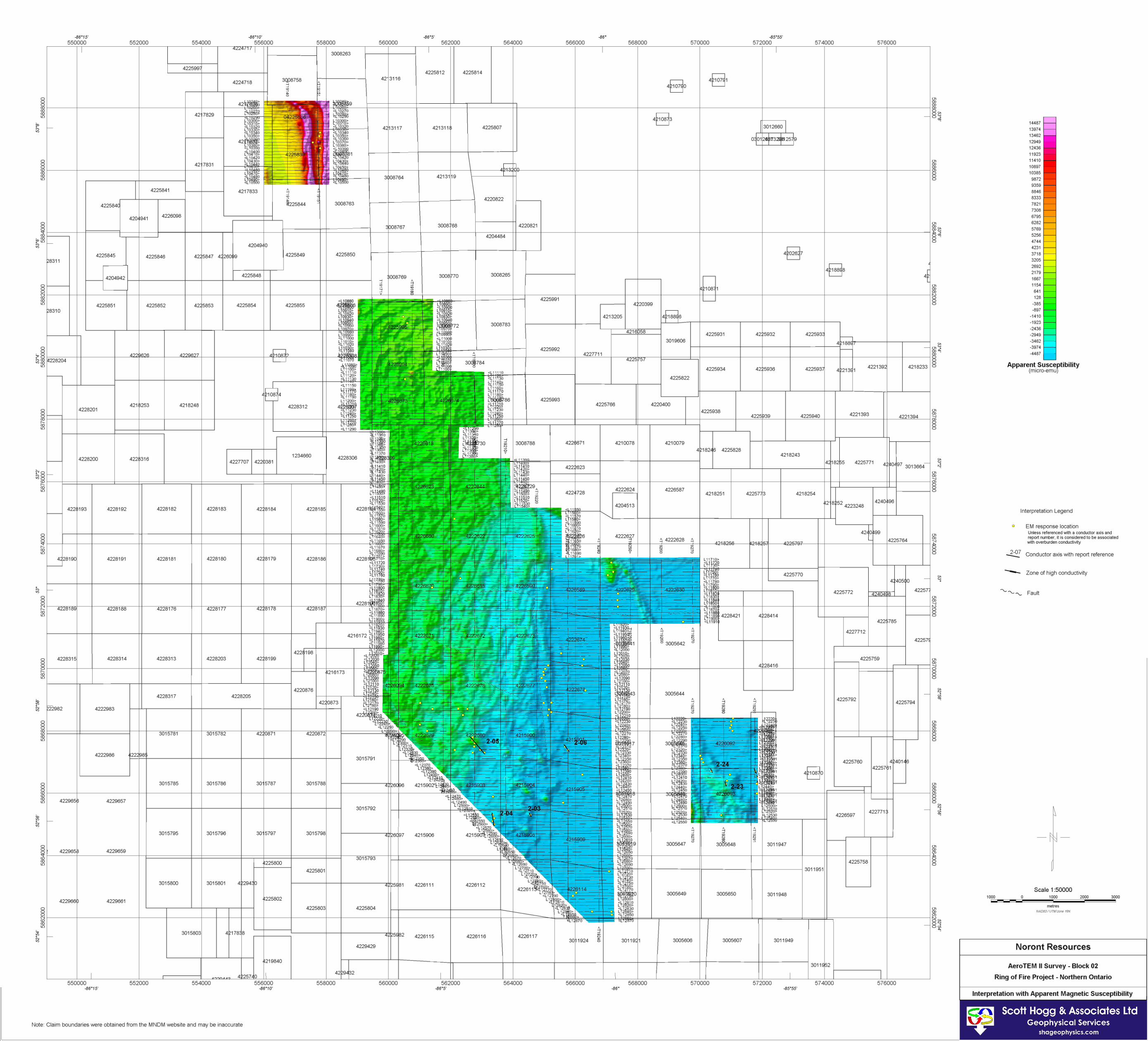
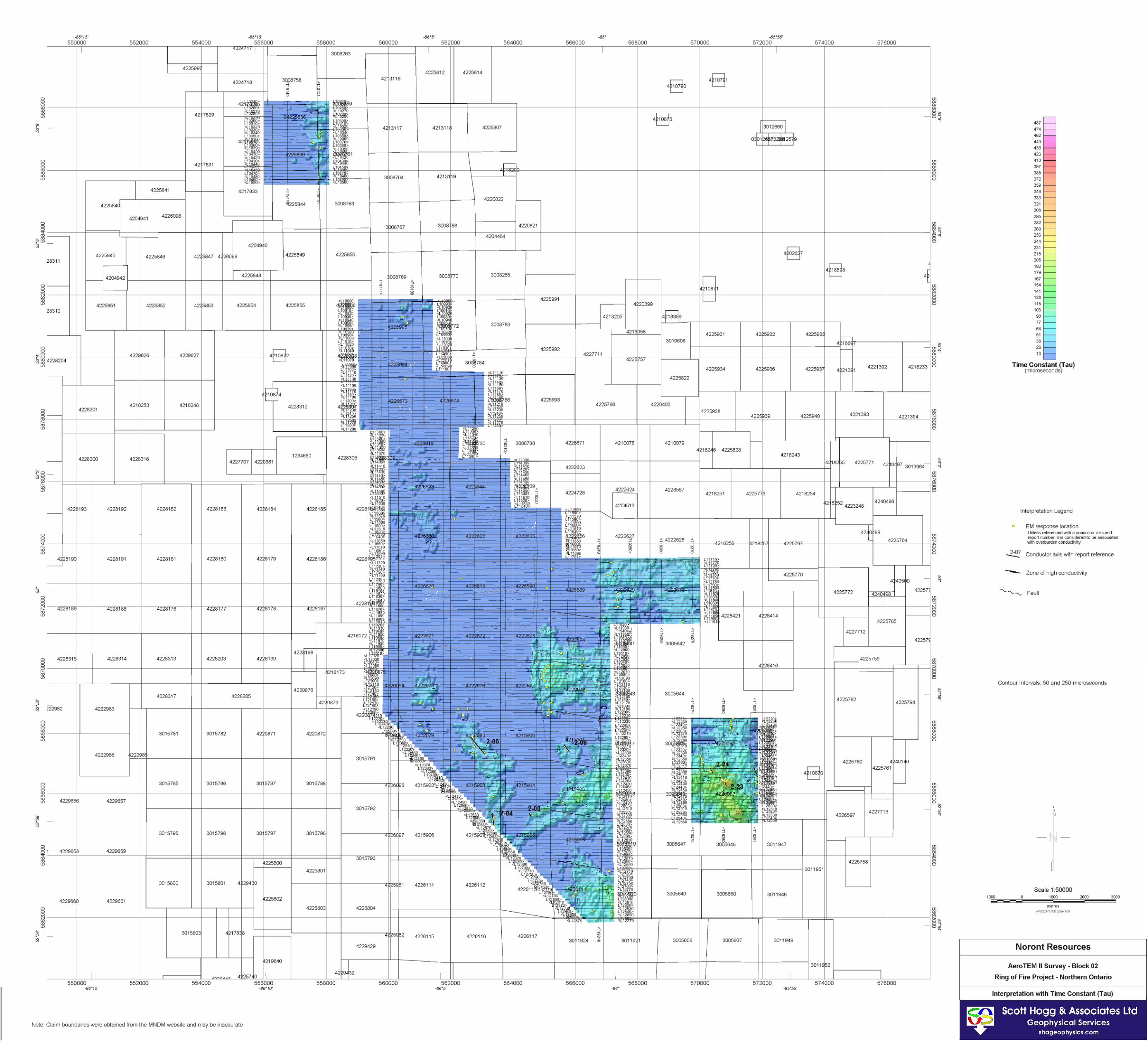
-86'15'

550000

I

552000 554000 _86'10'

556000 4LL41 1 I I

4224718

o o o ~~------r----------------r----------~----r-----r---~E~\~§i~g __ co ,L (OL~

o o o (fJ IX]

tB

,on.ln. 1

4225841

4226098

-- -

4217833

3Q08758 j

'" ,. o

j

'" ,. 11225844

558000

3008263

i

t .~

~ .~ L ~

~ ~~ ; I-~----I 3008763

_86'5'

560000 562000

4225812 42' 3116

42 3117 421311

"I)UOlb4 42131 9

4225814

564000

4225807

.C [

4220822

_86'

566000 568000 570000

I

_85'55'

572000

I

574000 576000

-

Ul 00 00 m o 8

o Ul

D~====~-t-1=========t~==t====f------+----t----~-1--------r----f=========f=P====~=====r---1~UUO~11~'01 __ -1 ____ ~"U~UOI~OO ____ +--'~4<W~11~4~22=0~8~2~1t-______ -1 ________________ +----------------1----------------+---------------------------------+---------~00~ ~ ~~ _ ~ 4204484 8 ~ ~ L() 0 Ol -

4225845 4225846 I( 4225849 4225850 28311

~--~4204942~_r----------~----r_--~--~--42-2-5-84-8_r~------------+_r_--------~,

o o o IX]

"IX] co

o o o N "IX] co

o o o (fJ (fJ IX] co

o o

~ tB

=

-

-

4225851

4228201

4228200

4228192

4228191

4228314

4222983

4222986

4229657

4229659

4229661

I 550000

_86'15'

4225852

421 ,253

422,316

4228182

4228181

4228313

4228317

3015785

3015795

3015800

552000

4225854

4218248

4228183 42:'8184

4228180 42:'8179

4:2:2B1! (

4228203

4228205

3015786 OU 0101

3015796 OU 01~1

3015801

3015803 42178:18

554000

1219840

556000 _86' 10'


4225855

4228312

1234660

4228185

4228186

42211198

3015788

3015798

4225801

558000

4228306

~. ~'

~~ 4216172 k

3015791

3015792

3015793

4229429

j )UUOIO" (, "uue' IU

'" ~ 3008265

-; i!i

-

560000

--

-

4225991

3008783

4213205

Ul 00 00 " o o o

4: P ""-----1 4225931 4225933

H~i~ ~ 3019606 4 ~1 uRuR,O;-----t--,-------1 - 4225992 f----+-----------+-----+------+-------------fc- - g: ~

~t-~30~~t7~84~----~+---------i-~~11~~-~4220~15~)~7--~====~~-------+---i-----+---------i--t------t--+---~~ ~~~~~~ 0 <L 10 4225934 4225937 4~213~ 1 422139: 4218233

-

+r-er-r

-

-

!D

-

--

4225822

4225993 4225766 4220400

3008788 42215671 4210078 4210079

4225938 4221393

4218243

4221394 Ul 00 --.j 00 o o o

<J 'Qcb, 4225771 ~ ~~. [~j£ 4~~04~)7 3013664- ~

~r~l~9i'----~~: --+-----f-------------+----+--+-------+-----+-----+----+--------+-+--------++-+_ ~o -

~. 4222624 4226587 ~ ~. 4218251 "LLO, 4218254 ~

:Q ~ 4204513 ,~ 'v~ 4223248

~~--~--r-------___1----~--_,--~~------~~

4225770

- 4225772

4228414

. (f- '.-4227712 ~ j

~ ~ ~ ~

g 3005642 ;3

-- . . ",

-- It

3005644 4225792

I

4LLpiOO

-

4LLOI

U, 00 --.j

" o

1-----18

42257!

-

4225794

g: 1-9 ~--------------+_-----+------_r+_----_+----1~

o o o

4225760

421 c ~, c

- - , "'= _'L ~~Ud , ( -

Ul 00 m m o o o

<I 124mL ~ ~ _ j '/.i /

I<L~5~O"'-~ ~ f-

4215906

-L~2~\~i~n> 4226111 4226112

4226115 4226116 4226117 30 1924 30119:11

I 562000 564000 566000 568000

_86'S' _86'

j ~ ~ ~

3005647 ~ 3011947

~----------~--+_-----------1 3011951

3005649 3005650 3011948

3005606 3005607 3011949

3011952

I 570000 572000 574000

_85'55'

4226597 422771

4225758

1

576000

-

Ul 00 m El 8

~ ~

'"

1000 IiiiiiiiiiiI

487

474

462 449

436 423 410 397

385

372

359

346 333

321 308

295 282 269 256 244

231 218 205

192 179

167 154

141 128

115 103

90 77

64 51

38 26 13

Time Constant (Tau) (microseconds)





Fault

Contour Intervals: 50 and 250 microseconds

o Scale 1 :50000

1000


2000

Noront Resources

3000



Interpretation with Time Constant (Tau)

heli-borne em mag geophys survs rpt

Documents